Commun. Comput. Phys.doi: 10.4208/cicp.OA-2017-0007
Vol. 22, No. 3, pp. 863-888September 2017
Equilibrium Configurations of Classical Polytropic
Stars with a Multi-Parametric Differential Rotation
Law: A Numerical Analysis
Federico Cipolletta1,2, Christian Cherubini3,4,∗, Simonetta Filippi3,4,Jorge A. Rueda1,2,5 and Remo Ruffini1,2,5
1 Dipartimento di Fisica and ICRA, Sapienza Universita di Roma, P.le Aldo Moro 5,I–00185 Rome, Italy.2 ICRANet, Piazza della Repubblica 10, I–65122 Pescara, Italy.3 Unit of Nonlinear Physics and Mathematical Modeling, University CampusBio-Medico of Rome, Via A. del Portillo 21, I–00128 Rome, Italy.4 International Center for Relativistic Astrophysics-ICRA, University CampusBio-Medico of Rome, Via A. del Portillo 21, I–00128 Rome, Italy.5 ICRANet-Rio, Centro Brasileiro de Pesquisas Fısicas, Rua Dr. Xavier Sigaud 150,Rio de Janeiro, RJ, 22290–180, Brazil.
Received 13 January 2017; Accepted (in revised version) 27 February 2017
Abstract. In this paper we analyze in detail the equilibrium configurations of classicalpolytropic stars with a multi-parametric differential rotation law of the literature usingthe standard numerical method introduced by Eriguchi and Mueller. Specifically wenumerically investigate the parameters’ space associated with the velocity field char-acterizing both equilibrium and non-equilibrium configurations for which the stabilitycondition is violated or the mass-shedding criterion is verified.
PACS: 04.40.-b, 02.30.Jr, 02.60.-x
Key words: Free boundary problems, self-gravitating systems, numerical methods for partialdifferential equations.
1 Introduction
The problem of equilibrium of rotating self-gravitating systems, dating back to Newton’sPrincipia Mathematica studies on the Earth’s shape, still represents a very actual topic in
∗Corresponding author. Email addresses: [email protected] (F. Cipolletta), [email protected] (C.Cherubini), [email protected] (F. Filippi), [email protected] (J. A. Rueda), [email protected](R. Ruffini)
http://www.global-sci.com/ 863 c©2017 Global-Science Press
864 F. Cipolletta et al. / Commun. Comput. Phys., 22 (2017), pp. 863-888
the field of astrophysics. Its main target is to reconstruct the structure of rotating starsconsidered to be, in a first approximation, in hydrostatic equilibrium although more com-plicated hydrodynamical effects can be taken into account by using modern tools of nu-merical analysis. Historically the studies on spherical non rotating self-gravitating bodies(well summarized in the classical Chandrasekhar’s monograph on stellar structure [1])and on uniformly rotating ones in the case of incompressible fluids (deeply analysed tooin the companion Chandrasekhar’s monograph on ellipsoidal figures of equilibrium [2],as well as, for instance, in [4–12]) preceded the study of compressible uniformly rotatingpolytropic stars [3]. All of these studies were completed by a series of refined numer-ical integrations of the complicated field equations governing the problem, performedby the Japanese school, which specifically investigated the problem of self-gravitatingfluid’s shape bifurcations [13–20]. The next step then has been the inclusion of differen-tial rotation laws in the treatment, for instance in [21, 22], where rotation profiles wereconsidered admitting an exact integral relation leading to an analytical expression of thecentrifugal potential term in the hydrostatic equilibrium equation. In the literature it isknown that differential rotation plays an important role in modelling the rotating stars’structure, in particular for both initial and ending phases of the stars’ life. Most of theaforementioned works dealt with barotropic stars, i.e. configurations in which isopycnic(constant density) and isobaric (constant pressure) surfaces coincide, although it has beenrecently stressed the importance to consider also more general situations, like the baro-clinic one (in which isopycnic surfaces are inclined over isobaric ones) in order to obtainmore realistic configurations [23]. We have to point out also that although many recentpapers dealt with relativistic figures of equilibrium (see for instance e.g. [24] and refer-ences therein) in relation to the problem of modelling possible sources of gravitationalwaves, the initial step to investigate the effects of pure rotation is to consider the problemof classical figures of equilibrium first. In the present paper, we will analyse in detail i)a polytropic classical self-gravitating fluid, ii) with axial and equatorial symmetry andwith iii) a multi-parametric differential rotation law, which was proposed in [25] withouta systematic analysis of the possible configurations belonging to such a velocity profile.The main feature of this rotation profile is that, with respect to the study in [21], this onecan be considered as a generalization because it does not admit an analytical expressionfor the integral for centrifugal potential term. In addition, the presence of different free-parameters allows a more detailed study of the way in which the star rotates. By usingthe general method given in [21] in order to perform an analysis of the free-parameters’space, we identify the presence of possible bifurcation points in the configurations’ se-quences. The article is organized as follows. In Section 2, the numerical method byEriguchi and Mueller [21] is briefly reviewed, the multi-parametric differential rotationprofile taken by [25] is discussed and an analysis of possible instabilities which may bereached is performed. In Section 3, we show results locating stable configurations withinthe free-parameters’ space and focusing on how different values of parameters in therotation law could lead to different shaped configurations. The correctness of results ischecked and already known results of [21] are recovered. In Section 4 we summarize and
F. Cipolletta et al. / Commun. Comput. Phys., 22 (2017), pp. 863-888 865
discuss the results obtained. Finally, details on the numerical implementation and on thedefinitions of physical quantities adopted in the analysis are given in Appendix A.
2 Theoretical framework
2.1 The problem of equilibrium
In this section we review the general method for analyzing rotating and self-gravitatingfluids as presented in [21]. In this method the attention is focused on a configuration ofrotating and self-gravitating gas for which the equation of hydrostationary equilibrium,in its differential form, reads
−(~v·~∇)~v=~∇P
ρ+~∇Φg, (2.1)
being ~v, ρ, P and Φg respectively the fluid’s velocity, density, pressure and gravitationalpotential. The latter quantity must satisfy the Poisson’s equation, which for a generalconfiguration reads
∆Φg =
4πGρ, inside,
0, outside,(2.2)
being G the constant of gravitation. Note that left-hand side of Eq. (2.1) can be written as
−(~v·~∇)~v=−1
2~∇(~v·~v)−(~∇×~v)×~v, (2.3)
so that using Eq. (2.1) we get
~∇P
ρ+(~∇×~v)×~v=−
(~∇Φg+
1
2~∇(~v·~v)
), (2.4)
and as the right-hand side has null curl, one obtains the following integrability conditionfor Eq. (2.1)
~∇×
~∇P
ρ+(~∇×~v)×~v
=0. (2.5)
Writing explicitly the fluid’s velocity of a rotating gas in hydrostationary equilibrium incylindrical coordinates (,z,φ) as
~v=Ω(,z)eφ, (2.6)
one obtains that Eqs. (2.1) and (2.5) are respectively equivalent to
~∇P
ρ=−∇Φg+Ω2(,z)e, (2.7)
2Ω(,z)∂Ω(,z)
∂zeφ= ~∇
1
ρ×~∇P. (2.8)
866 F. Cipolletta et al. / Commun. Comput. Phys., 22 (2017), pp. 863-888
From Eq. (2.8), by assuming a barotropic Equation of State (EOS), P=P(ρ), we get
∂Ω
∂z=0, (2.9)
which is a well known sufficient condition (see [26]) for isopycnic (constant density) andisobaric (constant pressure) surfaces to be coincident. In addition, we also obtain that thecentrifugal term in Eq. (2.7) comes out from a potential which can be defined as
Φc =−∫
0′Ω2(′)d′. (2.10)
One can in principle investigate Eqs. (2.2) and (2.7) in their differential form, but this givesrise to problems in treating the boundary conditions to impose, which are the finitenessof Φg and P at the center of the star, the vanishing of Φg at infinity and the definition ofthe surface where P vanishes. On the other hand, by treating the integral form of theseequations, one can incorporate the boundary condition in an easier way. To do so, wehave to note that Φg at a point ~x, due to the presence of mass in the volume V, can bewritten as (see e.g. [27])
Φg(~x)=−G∫
V
ρ(~x′)
|~x−~x′|dV ′, (2.11)
which using spherical coordinates (r,θ,φ) together with axial and equatorial symmetries,is equal to
Φg(r,θ)=−4πG∫ π
2
0sin(θ′)dθ′
∫ rsurf(θ)
0r′2dr′
·∞
∑n=0
f2n(r,r′)P2n(cos(θ))P2n(cos(θ′))ρ(r′ ,θ′). (2.12)
Here we indicate with P2n(cos(θ)) the Legendre’s polynomial of order 2n computed incos(θ) and f2n are the Green’s functions (of even order), defined by
f2n(r,r′)=
r′2n
r2n+1 for r≥ r′,
r2n
r′2n+1 for r< r′.(2.13)
It is possible now to have Eq. (2.1) in its integral form, which can be written as
∫1
ρdP+Φg+Φc=C (const.) . (2.14)
The system to be solved is defined via Eq. (2.14) coupled to Eq. (2.12). But one still hasto insert the EOS and the boundary conditions to define the surface (a free boundaryproblem) of the figure of equilibrium, namely
ρ(rsurf)=0 (2.15)
F. Cipolletta et al. / Commun. Comput. Phys., 22 (2017), pp. 863-888 867
and a rotation law, that is a relation to express Ω as a function of the adopted coordinates,which will be used in the centrifugal potential term, Φc. The choice of the EOS relationis one the most delicate points in approaching the problem of equilibrium of rotatinggases from the physical point of view. In fact, different EOSs can result in very differentconfigurations of equilibrium of rotating stars. For the sake of simplicity we supposethat the gas we are modelling is perfect, in the sense that it is composed of non-interactingparticles (i.e. the effects of interacting particles is negligible, thus we can neglect viscosityimplicated by energy dissipation during motion due to the interaction between particles)and it is non-degenerate (see e.g. [27]). An EOS which in a first approximation is able tomodel this kind of physical properties is the polytropic one
P=Kρ1+ 1n , (2.16)
where K is the polytropic constant and n is the polytropic index. At this point, the onlymissing ingredient to numerically solve the system of equations (which we report in Ap-pendix A) is a rotation profile.
2.2 Multi-parametric differential rotation law
When integrating hydrostationary equilibrium equation together with Poisson’s equa-tion on a discretized numerical grid (see Appendix A for details) one should also supplya rotation law, i.e. a relation to express the angular velocity on each grid-point as a func-tion of the spatial variables. In particular, actually we are interested in the study of theaxisymmetric case, in which equatorial symmetry is also prescribed, thus a natural choiceof coordinates’ set will be the spherical one (r,θ,φ). In literature many cases have alreadybeen studied, taking into account both uniform rotation, i.e. Ω = const. (see e.g. [3]),and differential rotation, i.e. Ω = Ω(), being = rsin(θ) the cylindrical radius (seee.g. [22] and [21]). More precisely, in papers dealing with differential rotation, a single-free-parameter differential rotation law is chosen, i.e. where Ω() depends also on onesingle free parameter which allows to control how much differential is the rotation, in thesense that for a defined value the uniformly rotating case is recovered. We consider herea differential rotation law of the following kind (see Ref. [25]):
Ω()=Ω0e−B2
1+(
A
)2, (2.17)
being Ω0 the central angular velocity and A and B parameters which control the rotationlaw and that in a limiting case can reproduce uniform rotation. It is worth noting that theif A→∞, the rotation law tends to the one of [22], while if B=0, it is the so-called j-const.rotation law of [21]. Although it may seem that Ω0, A and B are all free-parameters, thereader will see that Ω0 is treated as an unknown by the method adopted, thus the actualfree-parameters’ number is two as the value of Ω0 is obtained from the choice of the axis

868 F. Cipolletta et al. / Commun. Comput. Phys., 22 (2017), pp. 863-888
ratio. We then require A,B≥ 0. It is useful to introduce dimensionless variables withinthe method, adopting the following relation:
F= kF F, (2.18)
where F is the physical quantity in real dimension, kF is the constant for non-dimensionalization and F is the quantity in dimensionless form. In particular, as in [21]we adopt non-dimensional constants as reported in Table 1, where n is the polytropic in-dex, K is the polytropic constant and G is the gravitational constant. Looking at Eq. (2.17)is evident that parameters A and B have dimensions of length and length−2 respectively,thus it is also useful to impose
A= ars, (2.19)
B=b
req2
, (2.20)
with rs being the radius of the spherical configuration and req the equatorial sphericalcoordinate radius, just like in [21] (for parameter A) and [22] (for parameter B). Themain problem in choosing differential rotation given by Eq. (2.17), is that the integralto compute the centrifugal potential term in the hydrostationary equilibrium equation(see Section 2) cannot be performed analytically. For this reason we have decided to
Table 1: Constants adopted to obtain dimensionless quantities from Eq. (2.18).
F kF F Physical Meaning
ρ ρc σn Density
P Kρ1+ 1
nc σn+1 Pressure
Ω2 [4πGρc] ν Squared Angular Velocity
Φg K(n+1)ρ1nc Ψ Gravitational Potential
r
[K(n+1)
4πG ρ1n−1c
] 12
ξ Spherical Radius
M 4π[
K(n+1)4πG
] 32
ρ3−n2n
c M Mass
J[K(n+1)]
52
4πG2 ρ5−2n
2nc j Angular Momentum
IΩ[K(n+1)]
52
[4π]32 G
52
ρ5−3n
2nc I Moment of Intertia
T[K(n+1)]
52
[4π]12 G
32
ρ5−n2n
c T Kinetic Energy
W[K(n+1)]
52
[4π]12 G
32
ρ5−n2n
c W Gravitational Potential Energy
U[K(n+1)]
52
[4π]12 G
32
ρ5−n2n
c U Thermal Energy
F. Cipolletta et al. / Commun. Comput. Phys., 22 (2017), pp. 863-888 869
perform a numerical integration (via trapezoidal method) on an artificial numerical gridfor each axis distance from the particular grid-point in which to compute the value ofcentrifugal potential, considering a very large set of Ncyl points (namely Ncyl = 1000 foreach grid-point and Ncyl = 10000 to find the integration constant). With such numericalgrid in the cylindrical radial coordinate, the aforementioned numerical integration forthe centrifugal potential is able to properly reproduce already known results [21] (seeSection 4). This allows us to study in a general numerical way every kind of differentialrotation law, without requiring an analytical form for centrifugal potential.
2.3 Stability
As already pointed out in [22], an important condition which the chosen rotation lawshould satisfy is the stability condition against axisymmetric perturbation, provided bythe Solberg-Høiland criterion,
d[2Ω()
]
d>0, (2.21)
which states that the angular momentum per unit mass 2Ω must increase outwards(c.f. [22], [26] and [27]), i. e. going from the pole to the equator (for a complete deriva-tion of this criterion we refer to [28]). Thus, when choosing a rotation law, one mustalways verify that Eq. (2.21) is satisfied in order to guarantee stability. Using Eq. (2.17) inEq. (2.21), it is easy to check that this condition is equivalent to
B2A2+B4−A2<0, (2.22)
which, using definitions given in Eqs. (2.19), (2.20) and in Table 1 for r and simplifyingfor a factor Kr
2, in dimensionless form reads as:
b
ξeq2˜2a2ξs
2+b
ξeq2˜4−a2ξs
2<0, (2.23)
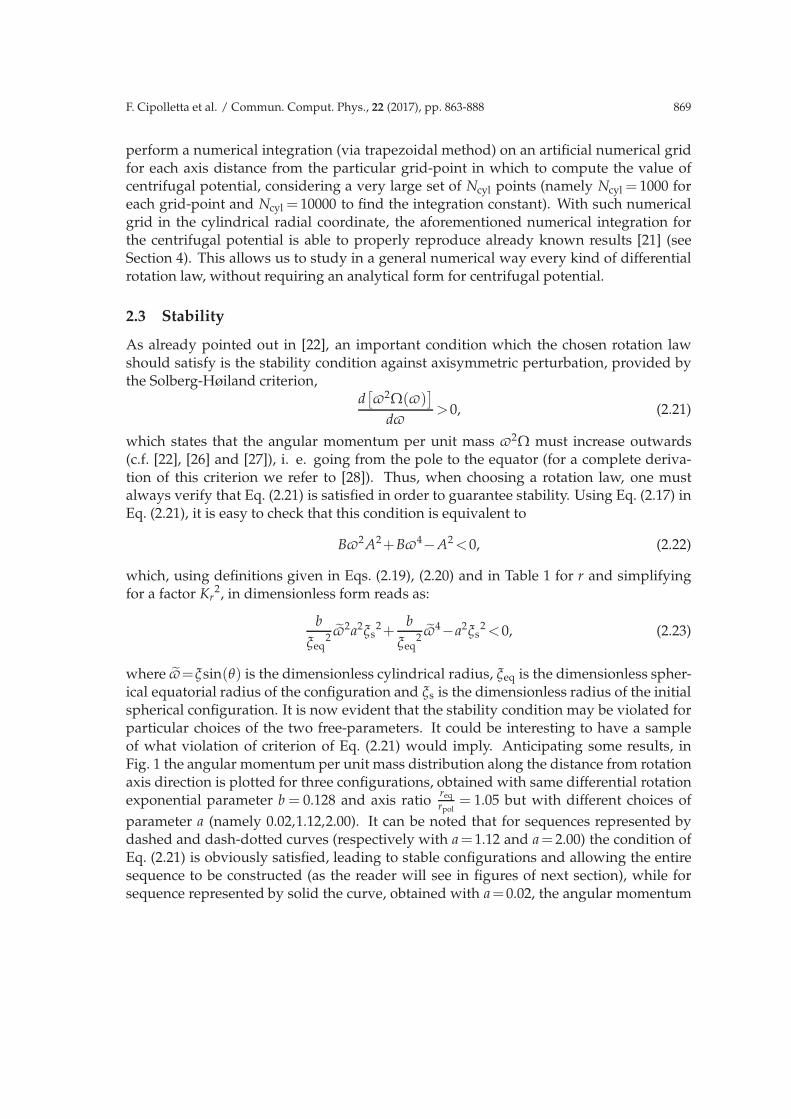
where ˜=ξsin(θ) is the dimensionless cylindrical radius, ξeq is the dimensionless spher-ical equatorial radius of the configuration and ξs is the dimensionless radius of the initialspherical configuration. It is now evident that the stability condition may be violated forparticular choices of the two free-parameters. It could be interesting to have a sampleof what violation of criterion of Eq. (2.21) would imply. Anticipating some results, inFig. 1 the angular momentum per unit mass distribution along the distance from rotationaxis direction is plotted for three configurations, obtained with same differential rotationexponential parameter b = 0.128 and axis ratio
req
rpol= 1.05 but with different choices of
parameter a (namely 0.02,1.12,2.00). It can be noted that for sequences represented bydashed and dash-dotted curves (respectively with a=1.12 and a=2.00) the condition ofEq. (2.21) is obviously satisfied, leading to stable configurations and allowing the entiresequence to be constructed (as the reader will see in figures of next section), while forsequence represented by solid the curve, obtained with a=0.02, the angular momentum
870 F. Cipolletta et al. / Commun. Comput. Phys., 22 (2017), pp. 863-888
Figure 1: Angular momentum per unit mass distribution along distance from rotation axis for three sample
sequences obtained with same choice of parameter b=0.128 and axis ratioreq
rpol=1.05, but different choices of
parameter a=0.02, 1.12, 2.00.
per unit mass distribution is slowly decreasing. The stability condition given by Eq. (2.21)is not the only one to be controlled. In fact, another physical limit for the rotation whichis worth to take into account is the mass-shedding limit, namely the point in which therotation becomes too fast to allow stability. As already presented in [3] or [26] the afore-mentioned limit for equilibrium configurations in the axisymmetric case occurs when theeffective gravity of the surface at the equator becomes zero, which means that the gravi-tational force is perfectly balanced by the centrifugal one (and vice-versa). Actually, if theangular velocity would increase further after this condition is reached, a portion of the to-tal mass should begin to shed from the star, because the centrifugal force would becomegreater than the gravitational one (the so-called “mass-shedding”). Using a polytropicEOS and the constants for dimensionless form given by Table 1, one gets the followingcriterion for dimensionless effective gravity
geq eff=∂σ
∂ξ
(ξsurf eq,
π
2
)≤0, (2.24)
necessary to avoid mass-shedding.
3 Results
3.1 Differentially rotating polytropes
In the following analyses, we have specifically adopted for the polytropic relation ofEq. (2.16) the value n= 1.5. Adopting a multi-parametric differential rotation law, such
F. Cipolletta et al. / Commun. Comput. Phys., 22 (2017), pp. 863-888 871
the one given in Eq. (2.17), it is possible to have a very detailed control on the way thestar rotates. It is interesting to understand the different figures of equilibrium whichcould result from different choices of these control parameters. Summarizing, to per-form such an analysis, one can use the method given in [21] to build several equilibriumsequences, each obtained by a fixed change in the axis ratio from one configuration to an-other (see Section 2), taking into account the Solberg-Høiland criterion in Eq. (2.21) andthe mass-shedding condition given in Eq. (2.24). Thus, we decided to fix initial extremafor parameters value, namely amin, amax, bmin and bmax and to compute respectively Na
and Nb linearly equally spaced parameter’s values between these extremes. Explicitly,the parameters value are given by the following equation:
pk = pmin+
((pmax−pmin)×
(k−1)
(Np−1)
)for k=1,··· ,Np, (3.1)
where with letter p the parameter’s name is intended, namely a or b. After having fixedthe set of values for free-parameters, several sequences can be computed starting from thespherical configuration until some kind of instability is reached. However we notice thatit is possible that none of the two instability condition could be reached, thus we decidedto stop the computations when 101 configurations have been built (this in order to limitthe computation time). Precisely, the maximum axis ratio of equilibrium configurationswhich is reached in this way is (1.05)101 ∼138.07.
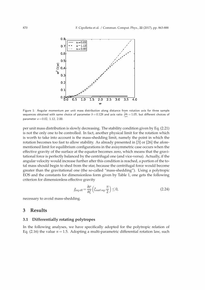
In Fig. 2 the kind of instability reached (after the entire sequence is computed) for eachchoice of the two rotational parameters is represented, with color convention given in the
Figure 2: Resulting equilibrium configurations for different choices of rotational parameters b and a of Eq. (2.17),obtained with 15-angular times 40-radial points in the numerical grid. Colour convention is: green is for mass-shedding criterion violation, yellow is for Solberg-Høiland criterion violation, blue is for concave hamburgerconfigurations, which after 101 configurations did not violate any stability criterion and purple is for concavehamburger configuration which reach mass-shedding at equator.
872 F. Cipolletta et al. / Commun. Comput. Phys., 22 (2017), pp. 863-888
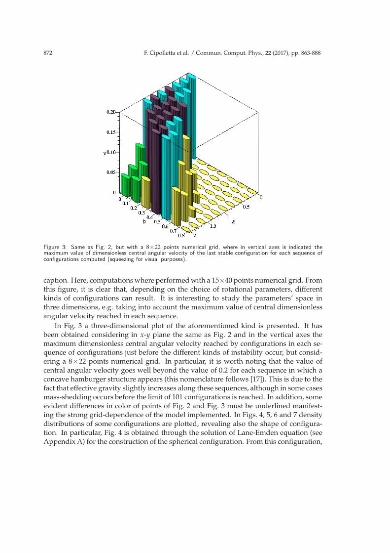
Figure 3: Same as Fig. 2, but with a 8×22 points numerical grid, where in vertical axes is indicated themaximum value of dimensionless central angular velocity of the last stable configuration for each sequence ofconfigurations computed (squeezing for visual purposes).
caption. Here, computations where performed with a 15×40 points numerical grid. Fromthis figure, it is clear that, depending on the choice of rotational parameters, differentkinds of configurations can result. It is interesting to study the parameters’ space inthree dimensions, e.g. taking into account the maximum value of central dimensionlessangular velocity reached in each sequence.
In Fig. 3 a three-dimensional plot of the aforementioned kind is presented. It hasbeen obtained considering in x-y plane the same as Fig. 2 and in the vertical axes themaximum dimensionless central angular velocity reached by configurations in each se-quence of configurations just before the different kinds of instability occur, but consid-ering a 8×22 points numerical grid. In particular, it is worth noting that the value ofcentral angular velocity goes well beyond the value of 0.2 for each sequence in which aconcave hamburger structure appears (this nomenclature follows [17]). This is due to thefact that effective gravity slightly increases along these sequences, although in some casesmass-shedding occurs before the limit of 101 configurations is reached. In addition, someevident differences in color of points of Fig. 2 and Fig. 3 must be underlined manifest-ing the strong grid-dependence of the model implemented. In Figs. 4, 5, 6 and 7 densitydistributions of some configurations are plotted, revealing also the shape of configura-tion. In particular, Fig. 4 is obtained through the solution of Lane-Emden equation (seeAppendix A) for the construction of the spherical configuration. From this configuration,
F. Cipolletta et al. / Commun. Comput. Phys., 22 (2017), pp. 863-888 873
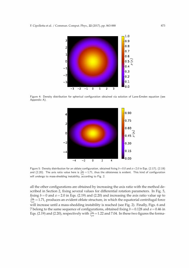
Figure 4: Density distribution for spherical configuration obtained via solution of Lane-Emden equation (seeAppendix A).
Figure 5: Density distribution for an oblate configuration, obtained fixing b=0.0 and a=2.0 in Eqs. (2.17), (2.19)
and (2.20). The axis ratio value here isreq
rpol= 1.71, thus the oblateness is evident. This kind of configuration
will undergo to mass-shedding instability, according to Fig. 2.
all the other configurations are obtained by increasing the axis ratio with the method de-scribed in Section 2, fixing several values for differential rotation parameters. In Fig. 5,fixing b= 0 and a= 2.0 in Eqs. (2.19) and (2.20) and increasing the axis ratio value up toreq
rpol=1.71, produces an evident oblate structure, in which the equatorial centrifugal force
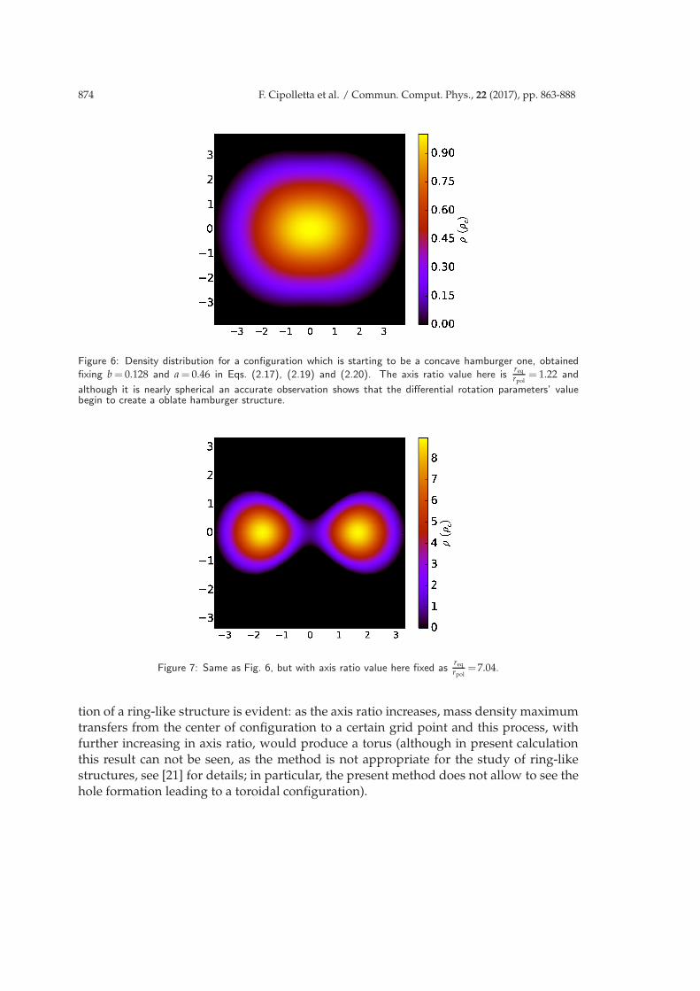
will increase until a mass-shedding instability is reached (see Fig. 2). Finally, Figs. 6 and7 belong to the same sequence of configurations, obtained fixing b=0.128 and a=0.46 inEqs. (2.19) and (2.20), respectively with
req
rpol=1.22 and 7.04. In these two figures the forma-
874 F. Cipolletta et al. / Commun. Comput. Phys., 22 (2017), pp. 863-888
Figure 6: Density distribution for a configuration which is starting to be a concave hamburger one, obtained
fixing b = 0.128 and a = 0.46 in Eqs. (2.17), (2.19) and (2.20). The axis ratio value here isreq
rpol= 1.22 and
although it is nearly spherical an accurate observation shows that the differential rotation parameters’ valuebegin to create a oblate hamburger structure.
Figure 7: Same as Fig. 6, but with axis ratio value here fixed asreq
rpol=7.04.
tion of a ring-like structure is evident: as the axis ratio increases, mass density maximumtransfers from the center of configuration to a certain grid point and this process, withfurther increasing in axis ratio, would produce a torus (although in present calculationthis result can not be seen, as the method is not appropriate for the study of ring-likestructures, see [21] for details; in particular, the present method does not allow to see thehole formation leading to a toroidal configuration).
F. Cipolletta et al. / Commun. Comput. Phys., 22 (2017), pp. 863-888 875
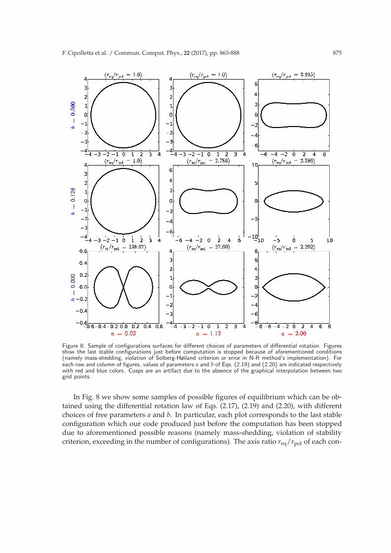
Figure 8: Sample of configurations surfaces for different choices of parameters of differential rotation. Figuresshow the last stable configurations just before computation is stopped because of aforementioned conditions(namely mass-shedding, violation of Solberg-Høiland criterion or error in N-R method’s implementation). Foreach row and column of figures, values of parameters a and b of Eqs. (2.19) and (2.20) are indicated respectivelywith red and blue colors. Cusps are an artifact due to the absence of the graphical interpolation between twogrid points.
In Fig. 8 we show some samples of possible figures of equilibrium which can be ob-tained using the differential rotation law of Eqs. (2.17), (2.19) and (2.20), with differentchoices of free parameters a and b. In particular, each plot corresponds to the last stableconfiguration which our code produced just before the computation has been stoppeddue to aforementioned possible reasons (namely mass-shedding, violation of stabilitycriterion, exceeding in the number of configurations). The axis ratio req/rpol of each con-

876 F. Cipolletta et al. / Commun. Comput. Phys., 22 (2017), pp. 863-888
figuration is reported in parentheses above each plot. A spherical figure means that theparticular choice of rotational parameter leads immediately to some kind of instability(the reader should refer specifically to Fig. 2). Before concluding this section, an impor-tant consideration must be done. Our code adopts the Newton-Raphson (N-R) methodas discussed in Ref. [29] in order to compute the solution of a set of non-linear equations.The code uses the LU decomposition method in order to invert the Jacobian matrix butwe found in some cases instabilities. In fact, the Newton-Raphson method implementedcould lead to local minima of the system, instead to an absolute one. For this reasonand because of the strong grid-dependence of Eriguchi and Mueller method, in somecases, the computation could be interrupted for some particular choices of rotational pa-rameters before one of the stopping conditions occurs. How can be possible to recoverthese missing result? In these cases the grid-dependence study helps us. In fact, onecould perform some cross-checks between results obtained using several grids and thisguarantees the accuracy of results presented. In particular, for results presented in thissection, we compared results obtained with 8×22 and 15×40 grids. We also report inTables 2-4, the physically relevant values of some of the sequences computed, exemplify-ing the different configurations of equilibrium obtained. It is worth noting that, althoughusually convergence may be recovered changing the initial guess, this is not possible forthe present situation, because the computation is always starting from the sphericallysymmetric configuration, obtained by the solution of Eq. (A.9). We also tried to reducethe step of axis ratio from one configuration to another (e.g. 1.01), but neither this couldgive any benefit to the convergence.
Table 2: Results of our numerical computations for an almost uniformly rotating sequence of equilibriumconfigurations obtained fixing b=0 and a=2.0. This sequence will end in mass-shedding.
ξeq
ξpolj2 T
|W|U|W|
M V.T.
1.000 0.000000 0.000000 0.500 2.710 9.55e−4
1.158 0.972e−3 0.2861e−1 0.472 2.994 4.87e−4
1.276 0.165e−2 0.4607e−1 0.454 3.156 4.24e−4
1.407 0.234e−2 0.6242e−1 0.438 3.323 3.93e−4
1.551 0.304e−2 0.7720e−1 0.423 3.488 3.71e−4
1.710 0.369e−2 0.9003e−1 0.410 3.643 3.59e−4
1.886 0.425e−2 0.1002000 0.400 3.774 3.48e−4
2.078 0.465e−2 0.1069000 0.393 3.867 3.23e−4
2.292 0.487e−2 0.1102000 0.390 3.934 3.28e−4
3.2 Numerical tests
To test our results with ones from literature, we will refer to tables presented in [21],for the so-called j-const rotation law, for choices of parameter A= 2.0rs, 0.2rs and 0.02rs
F. Cipolletta et al. / Commun. Comput. Phys., 22 (2017), pp. 863-888 877
Table 3: Results of our numerical computations for an almost uniformly rotating sequence of equilibriumconfigurations obtained fixing b=0.0 and a=1.12. This sequence will end in mass-shedding although it will alsotend to have a concave hamburger structure.
ξeq
ξpolj2 T
|W|U|W|
M V.T.
1.000 0.000000 0.000000 0.500 2.710 9.55e−4
1.477 0.307e−2 0.8168e−1 0.419 3.565 4.23e−4
2.407 0.853e−2 0.1873000 0.313 6.146 5.43e−4
3.920 0.133e−1 0.2583000 0.242 17.172 6.54e−4
6.385 0.166e−1 0.2763000 0.224 47.965 9.09e−4
10.401 0.187e−1 0.2867000 0.214 114.025 7.76e−4
16.943 0.201e−1 0.2949000 0.206 246.237 7.34e−4
27.598 0.212e−1 0.3016000 0.199 467.418 8.63e−4
Table 4: Results of our numerical computations for an almost uniformly rotating sequence of equilibriumconfigurations obtained fixing b= 0.383 and a= 1.34. This sequence will have a concave hamburger structureand it will not reach an instability although 101 configurations are computed.
ξeq
ξpolj2 T
|W|U|W|
M V.T.
1.000 0.000000 0.000000 0.500 2.710 9.55e−4
2.079 0.698e−2 0.1620000 0.338 5.299 5.23e−4
3.733 0.128e−1 0.2527000 0.248 16.536 7.49e−4
6.705 0.162e−1 0.2714000 0.229 54.776 7.77e−4
12.041 0.182e−1 0.2813000 0.219 150.250 1.083e−3
21.623 0.193e−1 0.2884000 0.212 378.059 9.17e−4
38.833 0.201e−1 0.2936000 0.207 915.252 6.78e−4
69.739 0.207e−1 0.2977000 0.207 2165.079 7.81e−4
which are reported in the following Tables 5, 6 and 7. Precisely the definition of quantitiesreported in each table is the same given in Table 1, with the exception of j2, the squareddimensionless angular momentum, which in paper [21] is defined as
j2=J2
(4π)43 M
103 σ
n3
max
, (3.2)
where dimensionless quantities are again defined in Table 1 and σmax is the maximumvalue of the dimensionless density of configuration. It is worth noting that with rotationlaw given in Eq. (2.17), keeping parameter B=0, one obtains exactly the same aforemen-tioned j-const rotation law. We will now turn to compare results of our computationswith values given in Tables 5, 6 and 7, plotting each quantity as a function of axis ratio inthe subsequent figures. Calculations have been performed using several numerical grids,
878 F. Cipolletta et al. / Commun. Comput. Phys., 22 (2017), pp. 863-888
Table 5: Results for numerical computations taken from [21] A=2.0rs.
ξeq
ξpolj2 T
|W|U|W|
V.T.
1.050 2.966e−4 9.183e−3 0.4911 5.7e−4
1.276 1.622e−3 4.530e−2 0.4549 4.8e−4
1.551 3.0228e−3 7.689e−2 0.4233 4.1e−4
1.886 4.244e−3 9.991e−2 0.4003 4.3e−4
2.292 4.766e−3 1.086e−1 0.3916 4.3e−4
Table 6: Results for numerical computations taken from [21] A=0.2rs.
ξeq
ξpolj2 T
|W|U|W|
V.T.
1.050 1.521e−4 7.236e−3 0.4931 5.7e−4
1.340 9.305e−4 4.323e−2 0.4570 5.3e−4
1.710 1.789e−3 7.514e−2 0.4251 4.9e−4
2.183 2.616e−3 1.022e−1 0.3991 5.0e−4
2.786 3.446e−3 1.220e−1 0.3783 5.1e−4
3.386 4.089e−3 1.356e−1 0.3647 5.0e−4
4.538 5.037e−3 1.528e−1 0.3475 4.6e−4
5.792 5.840e−3 1.651e−1 0.3352 4.6e−4
7.392 6.639e−3 1.762e−1 0.3240 4.7e−4
9.434 7.446e−3 1.864e−1 0.3138 4.8e−4
12.04 8.290e−3 1.961e−1 0.3042 4.6e−4
Table 7: Results for numerical computations taken from [21] A=0.02rs.
ξeq
ξpolj2 T
|W|U|W|
V.T.
1.050 3.393e−6 4.472e−4 0.4998 5.8e−4
1.710 5.310e−5 6.282e−3 0.4940 5.6e−4
2.786 1.253e−4 1.302e−2 0.4872 5.5e−4
3.920 1.896e−4 1.808e−2 0.4822 5.5e−4
6.385 3.098e−4 2.596e−2 0.4743 5.5e−4
9.434 4.392e−4 3.331e−2 0.4670 5.5e−4
14.64 6.332e−4 4.305e−2 0.4572 5.4e−4
25.03 9.597e−4 5.705e−2 0.4432 5.4e−4
38.83 1.315e−3 6.996e−2 0.4303 5.2e−4
60.24 1.771e−3 8.428e−2 0.4160 5.1e−4
89.01 2.277e−3 9.806e−2 0.4022 5.0e−4
F. Cipolletta et al. / Commun. Comput. Phys., 22 (2017), pp. 863-888 879
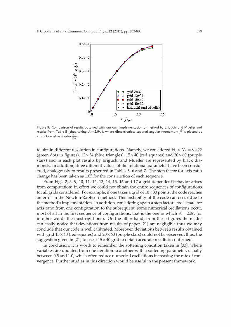
Figure 9: Comparison of results obtained with our own implementation of method by Eriguchi and Mueller andresults from Table 5 (thus taking A=2.0rs), where dimensionless squared angular momentum j2 is plotted as
a function of axis ratioreq
rpol.
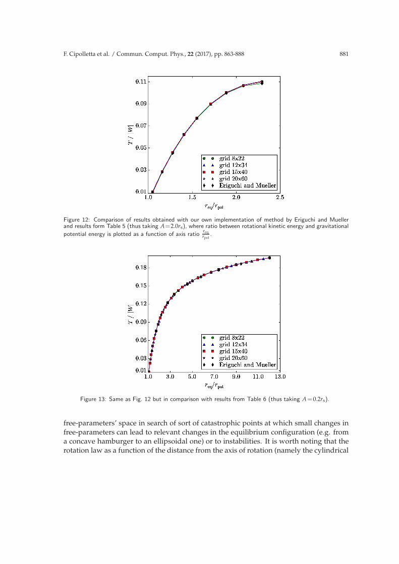
to obtain different resolution in configurations. Namely, we considered NT×NR =8×22(green dots in figures), 12×34 (blue triangles), 15×40 (red squares) and 20×60 (purplestars) and in each plot results by Eriguchi and Mueller are represented by black dia-monds. In addition, three different values of the rotational parameter have been consid-ered, analogously to results presented in Tables 5, 6 and 7. The step factor for axis ratiochange has been taken as 1.05 for the construction of each sequence.
From Figs. 2, 3, 9, 10, 11, 12, 13, 14, 15, 16 and 17 a grid dependent behavior arisesfrom computation: in effect we could not obtain the entire sequences of configurationsfor all grids considered. For example, if one takes a grid of 10×30 points, the code reachesan error in the Newton-Raphson method. This instability of the code can occur due tothe method’s implementation. In addition, considering again a step factor “too” small foraxis ratio from one configuration to the subsequent, some numerical oscillations occur,most of all in the first sequence of configurations, that is the one in which A= 2.0rs (orin other words the most rigid one). On the other hand, from these figures the readercan easily notice that deviations from results of paper [21] are negligible thus we mayconclude that our code is well calibrated. Moreover, deviations between results obtainedwith grid 15×40 (red squares) and 20×60 (purple stars) could not be observed, thus, thesuggestion given in [21] to use a 15×40 grid to obtain accurate results is confirmed.
In conclusion, it is worth to remember the softening condition taken in [33], wherevariables are updated from one iteration to another with a softening parameter, usuallybetween 0.5 and 1.0, which often reduce numerical oscillations increasing the rate of con-vergence. Further studies in this direction would be useful in the present framework.
880 F. Cipolletta et al. / Commun. Comput. Phys., 22 (2017), pp. 863-888
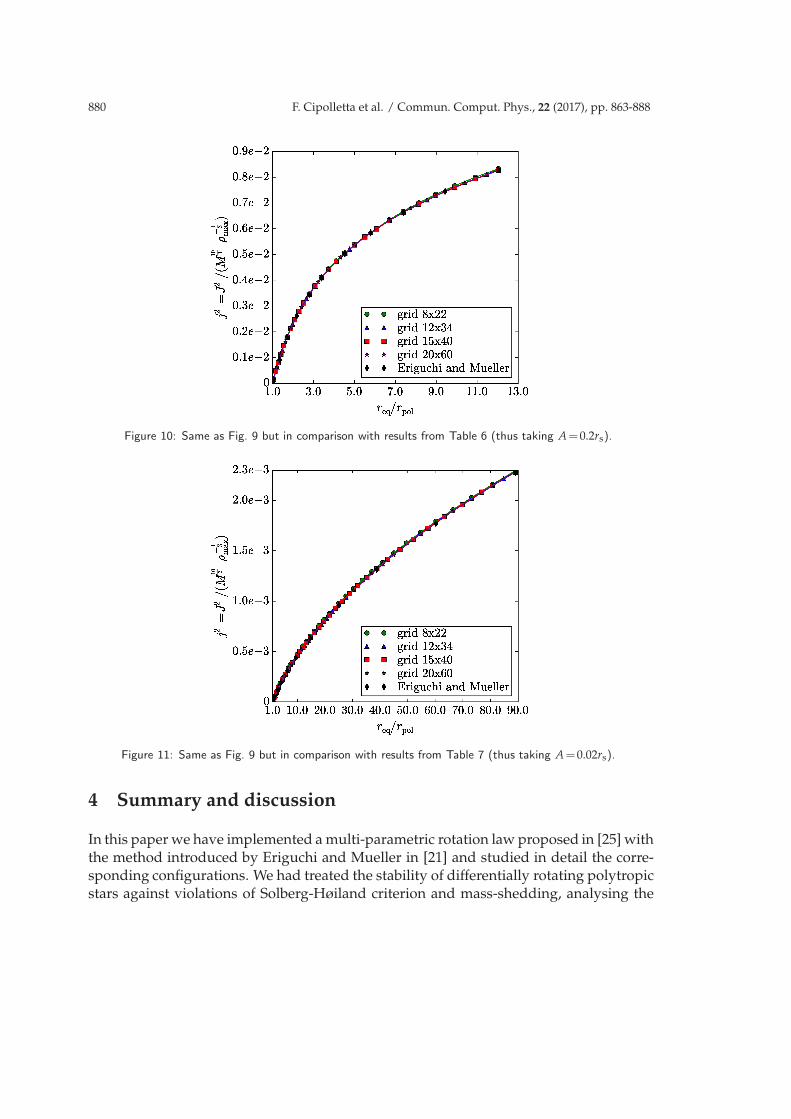
Figure 10: Same as Fig. 9 but in comparison with results from Table 6 (thus taking A=0.2rs).
Figure 11: Same as Fig. 9 but in comparison with results from Table 7 (thus taking A=0.02rs).
4 Summary and discussion
In this paper we have implemented a multi-parametric rotation law proposed in [25] withthe method introduced by Eriguchi and Mueller in [21] and studied in detail the corre-sponding configurations. We had treated the stability of differentially rotating polytropicstars against violations of Solberg-Høiland criterion and mass-shedding, analysing the
F. Cipolletta et al. / Commun. Comput. Phys., 22 (2017), pp. 863-888 881
Figure 12: Comparison of results obtained with our own implementation of method by Eriguchi and Muellerand results form Table 5 (thus taking A=2.0rs), where ratio between rotational kinetic energy and gravitational
potential energy is plotted as a function of axis ratioreq
rpol.
Figure 13: Same as Fig. 12 but in comparison with results from Table 6 (thus taking A=0.2rs).
free-parameters’ space in search of sort of catastrophic points at which small changes infree-parameters can lead to relevant changes in the equilibrium configuration (e.g. froma concave hamburger to an ellipsoidal one) or to instabilities. It is worth noting that therotation law as a function of the distance from the axis of rotation (namely the cylindrical
882 F. Cipolletta et al. / Commun. Comput. Phys., 22 (2017), pp. 863-888
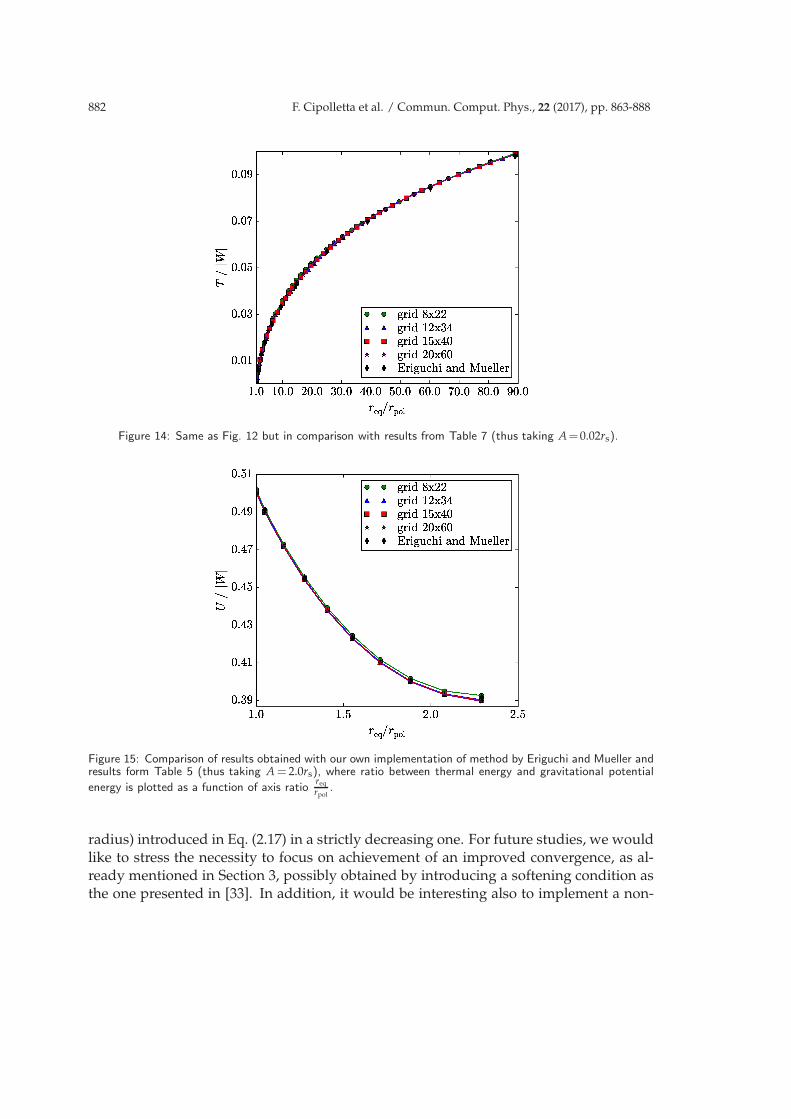
Figure 14: Same as Fig. 12 but in comparison with results from Table 7 (thus taking A=0.02rs).
Figure 15: Comparison of results obtained with our own implementation of method by Eriguchi and Mueller andresults form Table 5 (thus taking A= 2.0rs), where ratio between thermal energy and gravitational potential
energy is plotted as a function of axis ratioreq
rpol.
radius) introduced in Eq. (2.17) in a strictly decreasing one. For future studies, we wouldlike to stress the necessity to focus on achievement of an improved convergence, as al-ready mentioned in Section 3, possibly obtained by introducing a softening condition asthe one presented in [33]. In addition, it would be interesting also to implement a non-
F. Cipolletta et al. / Commun. Comput. Phys., 22 (2017), pp. 863-888 883
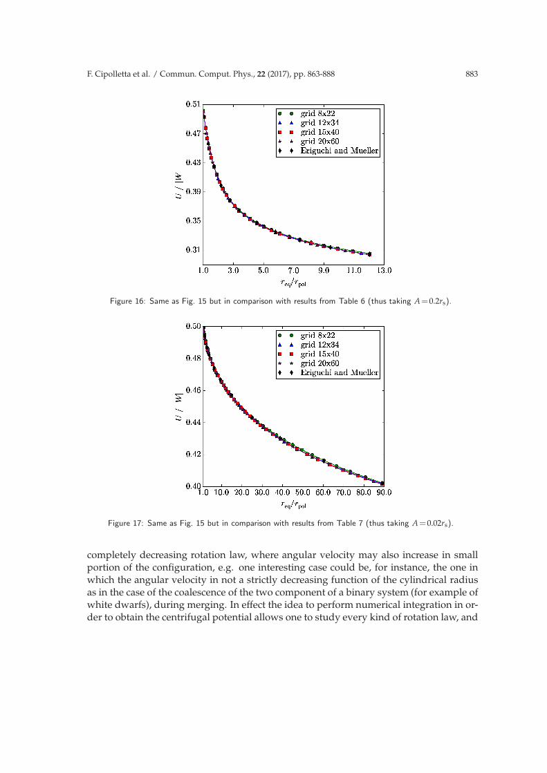
Figure 16: Same as Fig. 15 but in comparison with results from Table 6 (thus taking A=0.2rs).
Figure 17: Same as Fig. 15 but in comparison with results from Table 7 (thus taking A=0.02rs).
completely decreasing rotation law, where angular velocity may also increase in smallportion of the configuration, e.g. one interesting case could be, for instance, the one inwhich the angular velocity in not a strictly decreasing function of the cylindrical radiusas in the case of the coalescence of the two component of a binary system (for example ofwhite dwarfs), during merging. In effect the idea to perform numerical integration in or-der to obtain the centrifugal potential allows one to study every kind of rotation law, and
884 F. Cipolletta et al. / Commun. Comput. Phys., 22 (2017), pp. 863-888
studying the free-parameters space as in the way we propose, should in general allow tolocate instability points. We would also focus the attention to the fact that the methodpresented in [21] is in principle a general one, thus it should allow to consider differentkinds of EOS. In the present case, all previously presented results were obtained with an = 1.5 polytropic EOS, but it could also be interesting to treat the case of a numericalEOS, in which no analytical relation is known.
Appendix
A Numerical implementation and physical properties
A.1 Numerical method
Once an EOS and a rotation law are supplied, to solve the system of equations defined byEqs. (2.14), (2.15) and (2.12), in [21] a numerical method has been presented in which theinterior of the star is discretized in a mesh of points. Considering spherical coordinates,a grid is built dividing the domain into NT points along the θ-direction, and in NR pointsalong each r-direction. Grid points are defined as follows:
θi =π
2
i−1
NT−1, i=1,··· ,NT, (A.1)
rij = rj(θi)= rsurf(θi)j
NR, i=1,··· ,NT, j=1,··· ,NR. (A.2)
In particular, this grid does not consider the center of configuration because it has tobe treated separately from other points. Note in addition that the angular values varybetween 0 and π
2 , as equatorial symmetry is taken into account, while there is no depen-dence on the ϕ coordinate as expected by axial symmetry. Then, with the use of dimen-sionless variables as given in Table 1 it is possible to discretize the equations. Explicitlywriting the system for the fixed EOS and the rotation law, one can note that a model iscompletely determined by the prescription of polytropic constant K, central density ρc
and angular velocity Ω (this last condition holds in the case of uniform rotation; in caseof differential rotation one should instead fix the central value of angular velocity only,knowing that the values in all other points are given by the chosen rotation law). In themethod by Eriguchi and Mueller [21], it is stressed that fixing the angular velocity is notthe best way to solve the system of equation. Instead a better choice for numerical calcu-
lation is to fix the axis ratio, namelyreq
rpol=
rNR( π
2 )
rNR(0) =
ξeq
ξpol, the last equality obtained by the
introduction of the dimensionless radial coordinate. This condition gives one last equa-tion which will make the system solvable (see discussion on the number of equations andvariables at the end of the present section). Now we can write the discretized system ofequations, which will read as follows:
F. Cipolletta et al. / Commun. Comput. Phys., 22 (2017), pp. 863-888 885
(i) at the centre of configuration:
1+Ψcentre =C, (A.3)
Ψcentre=−NT
∑p=1
sin(θp)Θp
NR
∑q=1
ξpqRpqσnpq; (A.4)
(ii) at all the grid points:
σij+Ψij−1
2νξ2
ij sin(θi)2=C, (A.5)
Ψij =−NT
∑p=1
sin(θp)Θp
NR
∑q=1
ξ2pqRpqσn
pq
·∞
∑m=0
f2m(ξij,ξpq)P2n(cos(θi))P2n(cos(θp))σnpq; (A.6)
(iii) boundary conditions to define the surface:
σi,NR=0, for i=1,··· ,NT ; (A.7)
(iv) a last equation for the axis ratio:
ξNT ,NR
ξ1,NR
=λ. (A.8)
To note that in Eqs. (A.4) and (A.6), the integral over the volume is discretized. In particu-lar, the terms Θp and Rpq denote respectively angular and radial grid spacings multipliedby weight factors which depend on the numerical integration scheme which in radial di-rection is the Simpson rule while in angular direction is the trapezoidal rule. The systemof NT×(NR+1)+2 equations for the same number of unknowns (namely NT surfaceradii, NT×NR densities in each grid-point, the central value of angular velocity and theintegration constant which turns out to be the gravitational potential at the pole) can besolved using an iterative numerical method, such the one called the Newton-Raphson’s.The Newton-Raphson’s method in [21] starts from a spherical (non-rotating) configura-tion and gradually increases the axis ratio of the configuration by a constant factor near1 (for example 1.05 or less) to obtain a new configuration and then repeats the procedureuntil a certain stopping condition is reached. The computation of a spherically symmet-ric model (meant as the density distribution and the surface radius) of a polytropic starof index n is a well-known problem in astrophysics and it was studied by many authorsin the past (see e.g. [30]). The equation to solve, namely the Lane-Emden equation, reads
1
ξ2
∂
∂ξ
(ξ2 ∂σ(ξ)
∂ξ
)+σ(ξ)n =0, (A.9)
886 F. Cipolletta et al. / Commun. Comput. Phys., 22 (2017), pp. 863-888
where we have adopted the same notation for dimensionless variables as in the Section 1.One can solve Eq. (A.9) numerically, finding σ(ξ), imposing as initial conditions
σ(0)=1, (A.10a)
σ′(0)=0. (A.10b)
Through a Newton-Raphson iteration scheme, one can also find the zero of function σ(ξ),which represents the surface radius of the spherical solution. Finally, one can put ν=ν0=0and find C≡C0 with expression given by Eq. (A.5) in which Eq. (A.6) can be used.
A.2 Definition of relevant physical quantities
Once the density distribution and surface radii of a configuration are computed, onecould also evaluate its physical properties (cf. [27] and [31]). Firstly, the rotational kineticenergy of a rotating configuration can be found with the following expression
T=1
2
∫
Vρ2Ω2dV, (A.11)
where V is the volume, is the cylindrical radius (distance from the axis of rotation,thus = rsin(θ) when spherical coordinates are considered) and ρ represents as usualthe density. The gravitational potential energy, on the other hand, can be computed as
W=−1
2G∫
VρΦgdV, (A.12)
being G the constant of gravitation and Φg the gravitational potential, which can be com-puted with Eq. (2.11). The internal energy of the system reads as
U=1
γ−1
∫
VρdV, (A.13)
where γ is the polytropic adiabatic exponent defined as γ = 1+ 1n . Obviously the total
mass of the configuration is simply
M=∫
VρdV, (A.14)
while the total angular momentum is given by
J=∫
VρΩ2dV. (A.15)
Finally another quantity which is worth computing is the value of virial test, which in [21](just as in [32]) is expressed in the following form
V.T.=
∣∣∣∣(2T+W+3(γ−1)U)
W
∣∣∣∣, (A.16)
and it should be zero in order to have an accurate model.
F. Cipolletta et al. / Commun. Comput. Phys., 22 (2017), pp. 863-888 887
Acknowledgments
C.C. and S.F. acknowledge INdAM-GNFM and ICRANet for support. J.A.R. acknowl-edges partial support of the project No. 3101/GF4 IPC-11/2015 and the target programof the Ministry of Education and Science of the Republic of Kazakhstan.
References
[1] Chandrasekhar, S., 1967: An Introduction to the Study of Stellar Structure, Dover.[2] Chandrasekhar, S., 1987: Ellipsoidal Figures of Equilibrium, Dover.[3] James R. A., 1964: The Structure and Stability of Rotating Gas Masses, Astrophys. J., 140,
552-582.[4] Busarello, G., Filippi, S. and Ruffini R., 1988: Anisotropic tensor virial models for elliptical
galaxies with rotation or vorticity, Astron. Astrophys., 197, 91-104.[5] Busarello G., Filippi S. and Ruffini R., 1989: Anisotropic and inhomogeneous tensor virial
models for elliptical galaxies with figure rotation and internal streaming, Astron. Astro-phys., 213, 80-88.
[6] Busarello G., Filippi S. and Ruffini R., 1990: ’b-type’ spheroids, Astron. Astrophys., 227,30-32.
[7] Filippi S., Ruffini R. and Sepulveda A., 1990: Generalized Riemann configurations andDedekind’s theorem - The case of non-linear internal velocities, Astron. Astrophys., 231,30-40.
[8] Filippi, S.; Ruffini, R.; Sepulveda, A. 1990: On the generalization of Dedekind-Riemannsequences to nonlinear velocities., Europhys. Lett., 12, 735-740.
[9] Filippi, S.; Ruffini, R.; Sepulveda, A., 1990: Nonlinear velocities in generalized Riemannellipsoids., Nuovo Cim. B, 105, 1047-1054.
[10] Filippi S., Ruffini R. and Sepulveda A., 1991: Generalized Riemann ellipsoids - Equilibriumand stability, Astron. Astrophys., 246, 59-70.
[11] Filippi S., Ruffini R. and Sepulveda A., 1996: On the Implications of the nth-Order VirialEquations for Heterogeneous and Concentric Jacobi, Dedekind, and Riemann Ellipsoids,Astrophys. J., 460, 762
[12] Filippi S., Ruffini R. and Sepulveda A., 2002: Functional approach to the problem of self-gravitating systems: Conditions of integrability, Phys. Rev. D, 65, 044019.
[13] Eriguchi Y. and Sugimoto D. 1981: Another Equilibrium Sequences of Self-Gravitating andRotating Incompressible Fluid, Prog. Theor. Phys., 65, 1870-1875.
[14] Sugimoto D., Nomoto K. and Eriguchi Y. 1981: Stable Numerical Method in Computing ofStellar Evolution, Prog. Theor. Phys. Supp., 70, 115-131.
[15] Eriguchi Y. and Hachisu I., 1982: New Equilibrium Sequences Bifurcating from MaclaurinSequence, Prog. Theor. Phys., 67, 844-851.
[16] Eriguchi Y., Hachisu I. and Sugimoto D., 1982: Dumb-Bell Shape Equilibrium and MassShedding Pear-Shape of Self-Gravitating Incompressible Fluid, Prog. Theor. Phys., 67, 1068-1075.
[17] Hachisu I., Eriguchi Y., and Sugimoto D. 1982: Rapidly Rotating Polytropes and ConcaveHamburger Equilibrium, Prog. Theor. Phys., 68, 191-205.
[18] Hachisu I. and Eriguchi Y., 1982: Bifurcation and Fission of Three Dimensional, RigidlyRotating and Self-Gravitating Polytropes, Prog. Theor. Phys., 68, 206-221.
888 F. Cipolletta et al. / Commun. Comput. Phys., 22 (2017), pp. 863-888
[19] Eriguchi Y. and Hachisu I., 1983: Two Kinds of Axially Symmetric Equilibrium Sequences ofSelf-Gravitating and Rotating Incompressible Fluid, Prog. Theor. Phys., 69, 1131-1136.
[20] Hachisu I. and Eriguchi Y., 1983: Bifurcation and Phase Transitions of Self-Gravitating andUniformly Rotating Fluid, Mon. Not. R. Astron. Soc., 204, 583-589.
[21] Eriguchi Y. and & Mueller E.: 1985, A general computational method for obtaining equilibriaof self-gravitating and rotating gases, Astron. Astrophys., 146, 260-268.
[22] Stoeckly R., 1965: Polytropic Models with Fast, Non-Uniform Rotation, Astrophys. J., 142,208-228.
[23] Fujisawa K., 2015: A versatile numerical method for obtaining structures of rapidly rotatingbaroclinic stars: self-consistent and systematic solutions with shellular-type rotation, Mon.Not. R. Astron. Soc., 454, 3060-3072.
[24] Galeazzi F., Yoshida S. and Eriguchi Y., 2012: Differentially-rotating neutron star modelswith a parametrized rotation profile, Astron. Astrophys., 541, A156.
[25] Cherubini C., Filippi S., Ruffini R., Sepulveda A. and Zuluaga J. I., 2008: Non-HomogeneousAxisymmetric Models of Self-Gravitating Systems. The Eleventh Marcel Grossmann Meet-ing On Recent Developments in Theoretical and Experimental General Relativity, Gravita-tion and Relativistic Field Theories, 2340-2342.
[26] Tassoul, J.-L., 1978: Theory of rotating stars. Princeton Series in Astrophysics, PrincetonUniversity Press.
[27] Horedt, G. P., 2004: Polytropes - Applications in Astrophysics and Related Fields. KluwerAcademic Publishers.
[28] Maeder, A., 2009: Physics, Formation and Evolution of Rotating Stars. Astronomy and As-trophysics, Springer, Berlin.
[29] Press, W. H., Teukolsky, S. A., Vetterling, W. T. and Flannery, B. P., 1992: Numerical recipesin C. The art of scientific computing. Cambridge University Press, 2nd ed.
[30] Chandrasekhar S., 1933: The equilibrium of distorted polytropes. I. The rotational problem,Mon. Not. R. Astron. Soc., 93, 390-406.
[31] Chandrasekhar S., 1961: Hydrodynamic and hydromagnetic stability. Dover Publications.[32] Ostriker J. P. and Bodenheimer P., 1968: Rapidly Rotating Stars. II. Massive White Dwarfs,
Astrophys. J., 151, 1089-1098.[33] Uryu K., Limousin F., Friedman J.L., Gourgoulhon E. and Shibata, M., 2009: Nonconformally
flat initial data for binary compact objects, Phys. Rev. D, 80, 124004.
Recommended


![General Polytropic Magnetofluid under Self-Gravity: Voids ... · arXiv:0905.3490v1 [astro-ph.GA] 21 May 2009 General Polytropic Magnetofluid under Self-Gravity: Voids and Shocks](https://img.dokumen.tips/doc/110x75/60265c52e2443b1b721944af/general-polytropic-magnetoiuid-under-self-gravity-voids-arxiv09053490v1.jpg)