5
Energy Demand Analysis and Forecast
Wolfgang Schellong Cologne University of Applied Sciences
Germany
1. Introduction
Sustainable energy systems are necessary to save the natural resources avoiding
environmental impacts which would compromise the development of future generations.
Delivering sustainable energy will require an increased efficiency of the generation process
including the demand side. The architecture of the future energy supply can be
characterized by a combination of conventional centralized power plants with an increasing
number of distributed energy resources, including cogeneration and renewable energy
systems. Thus efficient forecast tools are necessary predicting the energy demand for the
operation and planning of power systems. The role of forecasting in deregulated energy
markets is essential in key decision making, such as purchasing and generating electric
power, load switching, and demand side management.
This chapter describes the energy data analysis and the basics of the mathematical
modeling of the energy demand. The forecast problem will be discussed in the context of
energy management systems. Because of the large number of influence factors and their
uncertainty it is impossible to build up an ‘exact’ physical model for the energy demand.
Therefore the energy demand is calculated on the basis of statistical models describing the
influence of climate factors and of operating conditions on the energy consumption.
Additionally artificial intelligence tools are used. A large variety of mathematical methods
and ideas have been used for energy demand forecasting (see Hahn et al., 2009, or Fischer,
2008). The quality of the demand forecast methods depends significantly on the
availability of historical consumption data as well as on the knowledge about the main
influence parameters on the energy consumption. These factors also determine the
selection of the best suitable forecast tool. Generally there is no 'best' method. Therefore it
is very important to proof the available energy data basis and the exact conditions for the
application of the tool.
Within this chapter the algorithm of the model building process will be discussed including
the energy data treatment and the selection of suitable forecast methods. The modeling
results will be interpreted by statistical tests. The focus of the investigation lies in the
application of regression methods and of neural networks for the forecast of the power and
heat demand for cogeneration systems. It will be shown that similar methods can be applied
to both forecast tasks. The application of the described methods will be demonstrated by the
heat and power demand forecast for a real district heating system containing different
cogeneration units.
www.intechopen.com

Energy Management Systems
102
2. Energy data management
2.1 Energy data analysis
Energy management describes the process of managing the generation and the
consumption of energy, generally to minimize demand, costs, and pollutant emissions.
The energy management has to look for efficient solutions for the challenges of
the changing conditions of the international energy economy which are caused by the
world wide liberalization of the energy market restricted by limited resources
and increasing prices (Doty & Turner, 2009). Computer aided energy management
combines applications from mathematics and informatics to optimize the energy
generation and consumption process. Information systems represent the basis for
controlling and decision activities. Because of the large number of relevant information an
efficient data management is to be used. Therefore mathematical analyzing and
optimizing methods are to be combined with energy data bases and with the data
management of the energy generation process. The detailed analysis of the main input
and output data of an energy system is necessary to improve its efficiency. Improving the
efficiency of energy systems or developing cleaner and efficient energy systems will slow
down the energy demand growth, make deep cut in fossil fuel use and reduce the
pollutant emissions.
Much of the energy generated today is produced by large-scale, centralized power plants
using fossil fuels (coal, oil, and gas), hydropower or nuclear power, with energy being
transmitted and distributed over long distances to the consumers. The efficiency of
conventional centralized power systems is generally low in comparison with combined heat
and power (CHP) technologies (cogeneration) which produce electricity or mechanical
power and recover waste heat for process use. CHP systems can deliver energy with
efficiencies exceeding 90%, while significantly reducing the emissions of greenhouse gases
and other pollutants (Petchers, 2003). Selecting a CHP technology for a specific application
depends on many factors, including the amount of power needed, the duty cycle, space
constraints, thermal needs, emission regulations, fuel availability, utility prices and
interconnection issues. The tasks and objectives of a local energy provider can be
summarized as follows:
Supply of the power and heat demand of the delivery district (additionally supply of
cool and other media as gas and water is possible)
Logistic management and provision of the primary fuels and of the support materials;
dispose of the waste materials
Portfolio management (i.e. buying and selling power at the power stock exchange)
Customer relationship management
Power plant and grid operation
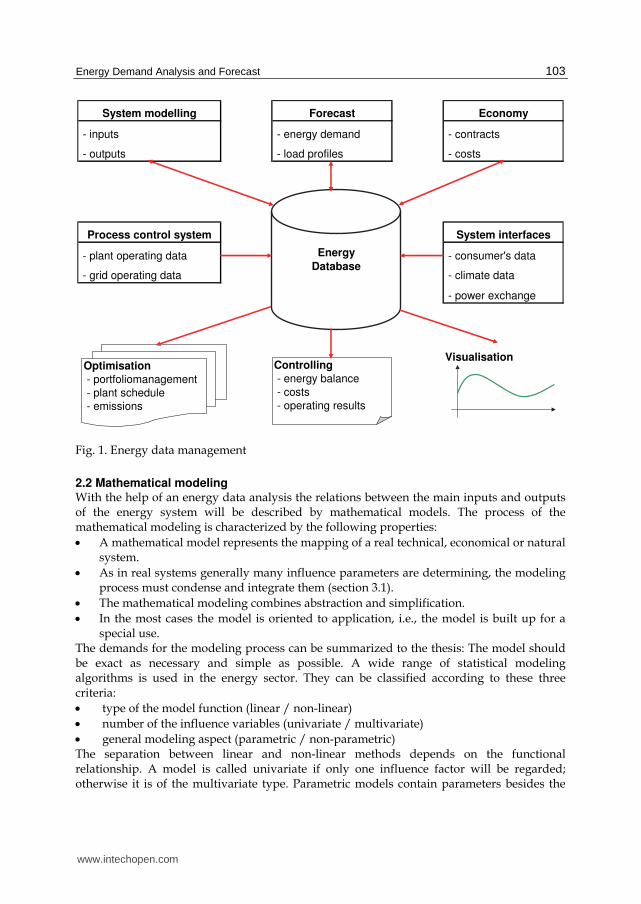
Fig. 1 shows the relationship model of the main input data resources and the data flow of
the energy data management. The energy database represents the heart of the energy
information system. The energy data management provides information for the energy
controlling including all activities of planning, operating, and supervising the generation
and distribution process. A detailed knowledge of the energy demand in the delivery
district is necessary to improve the efficiency of the power plant and to realize optimization
potentials of the energy system.
www.intechopen.com
Energy Demand Analysis and Forecast
103
- inputs - energy demand - contracts
- outputs - load profiles - costs
- plant operating data - consumer's data
- grid operating data - climate data
- power exchange
Visualisation
Forecast EconomySystem modelling
Process control system System interfaces
Energy
Database
Optimisation
- portfoliomanagement
- plant schedule
- emissions
Controlling
- energy balance
- costs
- operating results
Fig. 1. Energy data management
2.2 Mathematical modeling With the help of an energy data analysis the relations between the main inputs and outputs of the energy system will be described by mathematical models. The process of the mathematical modeling is characterized by the following properties:
A mathematical model represents the mapping of a real technical, economical or natural system.
As in real systems generally many influence parameters are determining, the modeling process must condense and integrate them (section 3.1).
The mathematical modeling combines abstraction and simplification.
In the most cases the model is oriented to application, i.e., the model is built up for a special use.
The demands for the modeling process can be summarized to the thesis: The model should be exact as necessary and simple as possible. A wide range of statistical modeling algorithms is used in the energy sector. They can be classified according to these three criteria:
type of the model function (linear / non-linear)
number of the influence variables (univariate / multivariate)
general modeling aspect (parametric / non-parametric) The separation between linear and non-linear methods depends on the functional relationship. A model is called univariate if only one influence factor will be regarded; otherwise it is of the multivariate type. Parametric models contain parameters besides the
www.intechopen.com

Energy Management Systems
104
input and output variables. The best known linear univariate parametric model is the classical single linear regression model (section 3.4). Non-parametric models as artificial neural networks (section 3.5) don't use an explicit model function. An explicit algebraic relationship between input and output can be described by the model
( , )y F x p (1)
where the function F describes the influence of the input vector x on the output variable y. The function F and the parameter vector p determine the type of the model. Regarding (1) there are two typically used modeling tasks: Simulation:
Calculate the outputs y for given inputs x and fixed parameters p, and compare the results. Parameter estimation (inverse problem): For given measurements of the input x and the output y calculate the parameters p so that the model fits the relation between x and y in a "best" way. The numerical calculation of the parameters of the regression model described in section 3.4 represents a typical parameter estimation problem.
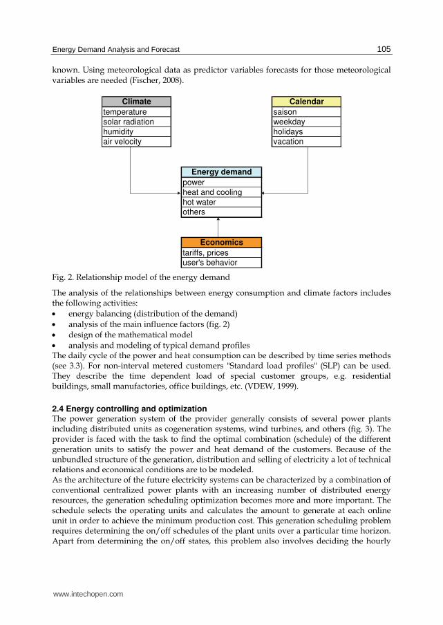
2.3 Energy demand analysis The energy consumption of the delivery district of a power plant depends on many different influence factors (fig. 2). Generally the energy demand is influenced by seasonal data, climate parameters, and economical boundary conditions. The heat demand of a district heating system depends strongly on the outside temperature but also on additional climate factors as wind speed, global radiation and humidity. On the other side seasonal factors influence the energy consumption. Usually the power and heat demand is higher on working days than at the weekend. Furthermore vacation and holidays have a significant impact on the energy consumption. Last but not least the heat and power demand in the delivery district is influenced by the operational parameters of enterprises with large energy demand and by the consumer’s behavior. Additionally the power and heat demand follow a daily cycle with low periods during the night hours and with peaks at different hours of the day. The quality of the energy demand forecast depends significantly on the availability of historical consumption data and on the knowledge about the main influence parameters on the energy demand. The functional relationship is non-linear and there are more or less complex interactions between different data types. Because of the large number of influence factors and their uncertainty it is impossible to build up an ‘exact’ physical model for the energy demand. Therefore the energy demand is calculated on the basis of mathematical models simplifying the real relationships as described in the previous section. Since no simple deterministic laws that relate the predictor variables (seasonal data, meteorological data and economic factors) on one side and energy demand as the target variable on the other side exist, it is necessary to use statistical models. A statistical model learns a quantitative relationship from historical data. During this training process quantitative relationships between the target variables (variables that have to be predicted) and the predictor variables are determined from historical data. Training data sets must be provided for known predictor target variables. From these example data the mathematical model is determined. This model can then be used to compute the values of the target variables as a function of the predictor variables for periods for which only the predictor variables are
www.intechopen.com
Energy Demand Analysis and Forecast
105
known. Using meteorological data as predictor variables forecasts for those meteorological variables are needed (Fischer, 2008).
Climate Calendar
temperature saison
solar radiation weekday
humidity holidays
air velocity vacation
Energy demand
power
heat and cooling
hot water
others
Economics
tariffs, prices
user's behavior
Fig. 2. Relationship model of the energy demand
The analysis of the relationships between energy consumption and climate factors includes the following activities:
energy balancing (distribution of the demand)
analysis of the main influence factors (fig. 2)
design of the mathematical model
analysis and modeling of typical demand profiles The daily cycle of the power and heat consumption can be described by time series methods (see 3.3). For non-interval metered customers "Standard load profiles" (SLP) can be used. They describe the time dependent load of special customer groups, e.g. residential buildings, small manufactories, office buildings, etc. (VDEW, 1999).
2.4 Energy controlling and optimization The power generation system of the provider generally consists of several power plants including distributed units as cogeneration systems, wind turbines, and others (fig. 3). The provider is faced with the task to find the optimal combination (schedule) of the different generation units to satisfy the power and heat demand of the customers. Because of the unbundled structure of the generation, distribution and selling of electricity a lot of technical relations and economical conditions are to be modeled. As the architecture of the future electricity systems can be characterized by a combination of conventional centralized power plants with an increasing number of distributed energy resources, the generation scheduling optimization becomes more and more important. The schedule selects the operating units and calculates the amount to generate at each online unit in order to achieve the minimum production cost. This generation scheduling problem requires determining the on/off schedules of the plant units over a particular time horizon. Apart from determining the on/off states, this problem also involves deciding the hourly
www.intechopen.com

Energy Management Systems
106
power and heat output of each unit. Thus the scheduling problem contains a large number of discrete (on/off status of plant units) and continuous (hourly power and heat output) variables.
Energymanagement
system
Energymanagement
system
Fig. 3. Distributed energy system (Maegard, 2004)
The objectives of the schedule optimization can be summarized as:
minimization of the fuel and operating costs
minimization of the distribution costs
reduction of CO2 emissions
optimization of the power trading The most important restrictions and boundary conditions of the optimization problem are given by (Schellong, 2006):
The generation system must satisfy the power and heat demand of the delivery district.
The power generation in a cogeneration system depends on the heat generation. The mathematical relations can be described in a similar way as described in 2.2.
There are a lot of boundary restrictions referring the capacity and the operating conditions of the generation units.
The operating schedule depends on the availability of the single generation units.
The system is influenced by constraints of the district heating network as well as of the electrical grid.
The generation system has to fulfill legal constraints referring emissions.
The optimization system is influenced by the delivery contracts and actual conditions of the energy trading at the energy stock exchange.
Thus the related mathematical optimization model has a very complex structure. Following the ideas described in section 2.2 the generation scheduling problem can be solved as a mixed integer linear optimization problem. The optimization results in an optimal schedule of the generation units using an optimal fuel mix and satisfying all restrictions. To realize
www.intechopen.com
Energy Demand Analysis and Forecast
107
this schedule the generation process must be supervised by the energy control system using the data management illustrated in fig. 1. It is obviously that these processes require the detailed knowledge of the energy demand of the delivery system. Especially for cogeneration systems it is important to know the coincidence of the power and heat demand. CHP units are only able to generate electricity efficiently, when the produced heat is simultaneously used on the demand side.
3. Energy demand forecast methods
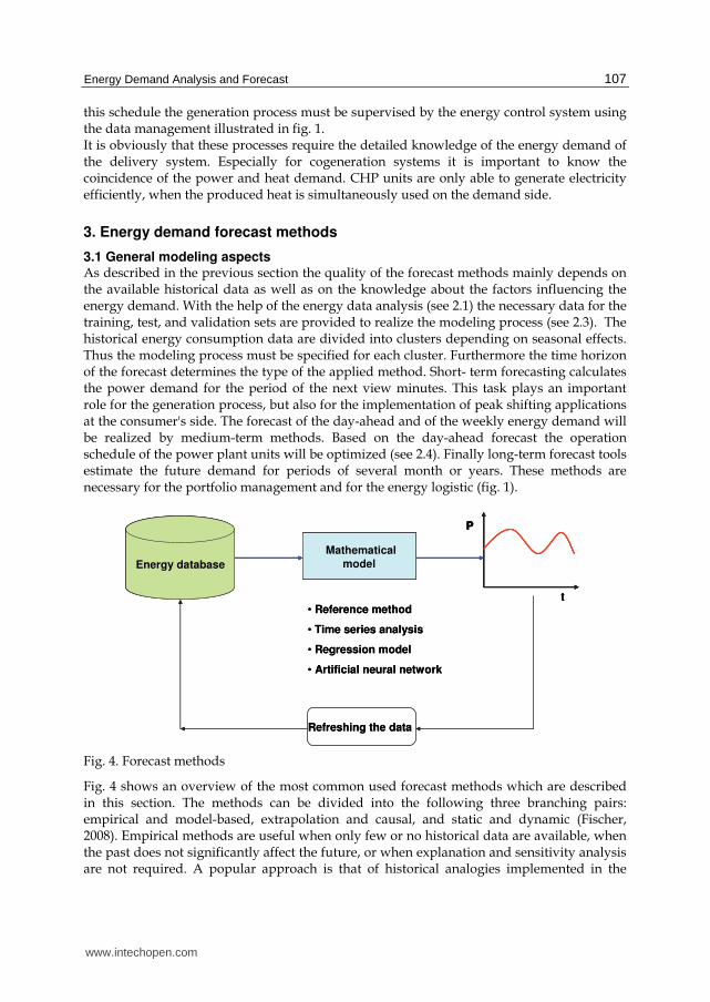
3.1 General modeling aspects As described in the previous section the quality of the forecast methods mainly depends on the available historical data as well as on the knowledge about the factors influencing the energy demand. With the help of the energy data analysis (see 2.1) the necessary data for the training, test, and validation sets are provided to realize the modeling process (see 2.3). The historical energy consumption data are divided into clusters depending on seasonal effects. Thus the modeling process must be specified for each cluster. Furthermore the time horizon of the forecast determines the type of the applied method. Short- term forecasting calculates the power demand for the period of the next view minutes. This task plays an important role for the generation process, but also for the implementation of peak shifting applications at the consumer's side. The forecast of the day-ahead and of the weekly energy demand will be realized by medium-term methods. Based on the day-ahead forecast the operation schedule of the power plant units will be optimized (see 2.4). Finally long-term forecast tools estimate the future demand for periods of several month or years. These methods are necessary for the portfolio management and for the energy logistic (fig. 1).
P
t
Energy database
Mathematical
model
• Reference method
• Time series analysis
• Regression model
• Artificial neural network
Refreshing the data
P
t
Energy database
Mathematical
model
P
t
P
t
Energy database
Mathematical
model
• Reference method
• Time series analysis
• Regression model
• Artificial neural network
Refreshing the data
Fig. 4. Forecast methods
Fig. 4 shows an overview of the most common used forecast methods which are described in this section. The methods can be divided into the following three branching pairs: empirical and model-based, extrapolation and causal, and static and dynamic (Fischer, 2008). Empirical methods are useful when only few or no historical data are available, when the past does not significantly affect the future, or when explanation and sensitivity analysis are not required. A popular approach is that of historical analogies implemented in the
www.intechopen.com
Energy Management Systems
108
reference method (see 3.2). Model-based methods use well-specified algorithms to process and analyze data. Extrapolation and causal methods are included in this category. Extrapolation methods are numerical algorithms that help forecasters find patterns in time-series observations of a quantitative variable. These are popular for short-range forecasting. This method is based on the assumption that a stable, systematic structure can describe the future energy demand. These models are characterized by the criteria described in section 2.2. A static forecast is used to predict the energy demand into the near future on the basis of actual data for the variables in the past or the present. On the other hand, a dynamic forecast can be used to make long term projections considering changes of the framework conditions during the forecast period.
3.2 Reference method The pure reference method works without a mathematical model. The basic idea of this simple method is to find a situation in an energy data base of historical data that is similar to the one that has to be predicted. A set of explanatory variables is defined and similarity between situations is measured by these variables. The method will be described by an example: To calculate the heat or power demand for a Monday, with a mean predicted temperature of +5 deg C the algorithm is simply looking in a data base for another Monday with a mean temperature close to +5 deg C. Thus the historical consumption data for that day are used as the prediction. For a long time this method has been the reference method for energy demand predictions especially for local energy providers, and surprisingly it is still widely used. The advantage of the method is that it is simple to implement. The results are easily to be interpreted. However the disadvantages are numerous. Although the implementation of the method seems to be straightforward, it becomes complicated if the number of criterions increases. If for instance hourly temperatures are used instead of daily mean temperature the measures of similarity are no longer so obvious. With an increasing number of explanatory variables, the probability to find no data set that is similar according to all criteria increases (Fischer, 2008). In practical applications the reference method is used in combination with some other
adaptation criteria depending on the behavior of the energy consumption in the past.
Additionally the reference method is supported by a regression model describing the
climate influence factors and/or time dependent energy consuming impacts caused by
production factors in industrial enterprises. On the other side the knowledge of the energy
consumption of selected historical reference days can improve the quality of model based
methods as will be described in section 4.
3.3 Time series analysis This method belongs to the category of the non-causal models of demand forecasting that do not explain how the values of the variable being projected are determined. Here the variable to be predicted is purely expressed as a function of time, neglecting other influence factors. This function of time is obtained as the function that best explains the available data, and is observed to be most suitable for short-term projections. A time series is often the superposition of the following terms describing the energy demand as time dependent output y(t):
Long-term trend variation (T)
Cyclical variation (C)
Seasonal variation (S)
www.intechopen.com
Energy Demand Analysis and Forecast
109
Irregular variation (R)
The trend variation T describes the gradual shifting of the time series, which is usually due
to long term factors such as changes in population, technology, and economy. The cyclical
component S represents multiyear cyclical movements in the economy. The periodic or
seasonal variation in the time series is, in general, caused by the seasonal weather or by
fixed seasonal events. The irregular component contains the residual of the time series if the
trend, cyclical and seasonal components are removed from the time series. These terms can
be combined to mixed time series model:
Additive model: y(t) = T(t) + S(t) + C(t) + R(t) (2)
Hybrid model: y(t) = T(t) x S(t) + R(t) (3)
In addition to the univariate time series analysis, autoregressive methods provide another modeling approach requiring only data on the previous modeled variable. Autoregressive
models (AR) describe the actual output yt by a linear combination of the previous time series yt-1, yt-2, . . . , yt-p and of an actual impact at:
yt = 1yt-1 + 2 yt-2 + . . . + p yt-p + at (4)
The autoregressive coefficients have to be estimated on the basis of measurements. The AR-
models can be combined with moving average models (MA) to ARMA models which have been firstly investigated by Box and Jenkins (Box & Jenkins, 1976).
The time series method has the advantage of its simplicity and easy use. It is assumed that the pattern of the variable in the past will continue into the future. The main disadvantage
of this approach lies in the fact that it ignores possible interaction of the variables. Furthermore the climate impacts and other influence factors are neglected.
3.4 Regression models
Regression models describe the causal relationship between one or more input variable(s)
and the desired output as dependent variable by linear or nonlinear functions. In the simplest case the univariate linear regression model describes the relationship between one
input variable x and the output variable y by the following formula:
y = f(x,a0,a1) = a0 + a1x (5)
Thus geometrically interpreted a straight line describes the relationship between y and x.
The shape of the straight line is determined by the so called regression parameters a0 and a1.
For given measurements x1, x2, . . . , xn and y1, y2, . . . , yn of the variables x and y the
parameters are calculated such that the mean quadratic distance between the measurements
yi (i=1, . . . ,n) and the model values ŷi on the straight line is minimized. That means the
following optimization problem is to be solved:
0 1
20 1 1
,1
( , ) ( ( , , ))i
n
i oa ai
Q a a y f x a a Min (6)
The calculated regression parameters represent a so called least squares estimation of the
fitting problem (Draper & Smith, 1998).
www.intechopen.com
Energy Management Systems
110
The regression model can be extended to a multivariate linear relationship where the output variable y is influenced by p inputs x1, x2, . . . , xp :
y = f(x,a) = a0 + a1x1 + a2x2 + . . . + apxp (7)
We define the following notations:
1
2
.
n
y
yy
y
1
2
.
p
a
aa
a
11 1
21 2
1
1 .
1 .
. . . .
1 .
p
p
n np
x x
x xX
x x
(8)
where the vector y contains the measurements of the output variable, a represents the vector of the regression parameters, and the matrix X contains the measurements xij of the ith observation of the input xj. Thus the least squares estimation of the multivariate linear regression problem will be obtained by solving the minimization task:
0 1
20 1 1 1 2 2
, ,...,1
( , ,..., ) ( ... ) ( ) ( )p
nnT
p i o i i p ipa a ai
Q a a a y a a x a x a x y Xa y Xa Min (9)
The least squares estimation of the regression parameter vector a represents the solution of the normal equation system referring to the minimization problem (9):
T TX Xa X y (10)
Regarding the special structure of this linear system, adapted methods like Cholesky or Housholder procedures are available to solve (10) using the symmetry of the coefficient matrix (Deuflhard & Hohmann, 2003). The model output can be described as
ˆ ˆy Xa (11)
where the vector ŷ contains the model output values ŷi (i=1, . . . , n) and a represents the vector of the estimated regression coefficients aj (j=1, . . . , p) as the solution of (10). The results of the regression analysis must be proofed by a regression diagnostic. That means we have to answer the following questions: Does a linear relationship between the input variables x1, x2, . . . , xp and the output y
really exist? Which input variables are really relevant? Is the basic data set of measurements consistent or are there any "out breakers"? With the help of the coefficient of determination B we can proof the linearity of the relationship.
2
1
2
1
ˆ( )
1
( )
n
i ii
n
ii
y ySSR
BSSY
y y
, (12)
where ˆi
y represent the calculated model values given by (11) and y is the arithmetic mean
value of the measured outputs yi. B ranges from 0 to 1. Values of B in the near of 1 indicate,
www.intechopen.com
Energy Demand Analysis and Forecast
111
that there exists a linear relationship between the regarded input and output. To identify the
most significant input variables the modeling procedure must be repeated by leaving one of
the variables from the model function within an iteration process. The coefficient of
determination and the expression s² = SSR/(n-p-1) indicate the significance of the left
variable. s² represents the estimated variance of the error distribution of the measured
values of y. Finally the analysis of the individual residuals ˆi i i
r y y gives some hints for the
existence of "out breakers" in the basic data set. Multivariate linear regressions are widely used in the field of energy demand forecast. They
are simple to implement, fast, reliable and they provide information about the importance of
each predictor variable and the uncertainty of the regression coefficients. Furthermore the
results are relatively robust. Nonlinear regression models are also available for the forecast.
But in this case the parameter estimation becomes more difficult. Furthermore the nonlinear
character of the influence variable must be guaranteed. Regression based algorithms
typically work in two steps: first the data are separated according to seasonal variables (e.g.
calendar data) and then a regression on the continuous variables (meteorological data) is
done. That means a regression analysis must be done for each seasonal cluster following the
algorithm:
Step 1. Analysis of the available energy data
Step 2. Splitting the historical energy consumption data into seasonal clusters
Step 3. Identifying the main meteorological factors on the energy demand as described in
section 2.3
Step 4. Regression analysis as described above
Step 5. Validation of the model (regression diagnostic)
Step 6. Integration of the sub models
The application of regression methods to the heat demand forecast for a cogeneration
system will be described in section 4.
3.5 Neural networks
Neural networks (NN) represent adaptive systems describing the relationship between
input and output variables without explicit model functions. NN are widely used in the
field of energy demand forecast (Schellong & Hentges, 2007). The basic elements of neural
networks (NN) are the neurons, which are simple processing units linked to each other with
directed and weighted connections. Depending on their algebraic sign and value the
connections weights are inhibiting or enhancing the signal that is to be transferred.
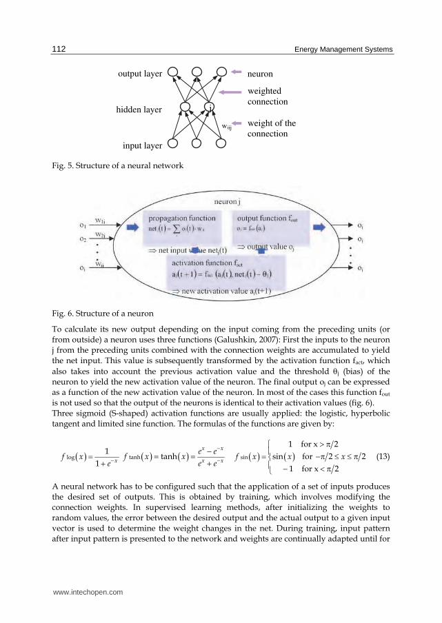
Depending on their function in the net, three types of neurons can be distinguished: The
units which receive information from outside the net are called input neurons. The units
which communicate information to the outside of the net are called output neurons. The
remaining units are called hidden neurons because they only send and receive information
from other neurons and thus are not visible from the outside. Accordingly the neurons are
grouped in layers. Generally a neural net consists of one input and one output layer, but it
can have several hidden layers (fig. 5).
The pattern of the connection between the neurons is called the network topology. In the
most common topology each neuron of a hidden layer is connected to all neurons of the
preceding and the following layer. Additionally in so-called feedforward networks the
signal is allowed to travel only in one direction from input to output (Fine, 1999).
www.intechopen.com
Energy Management Systems
112
Fig. 5. Structure of a neural network
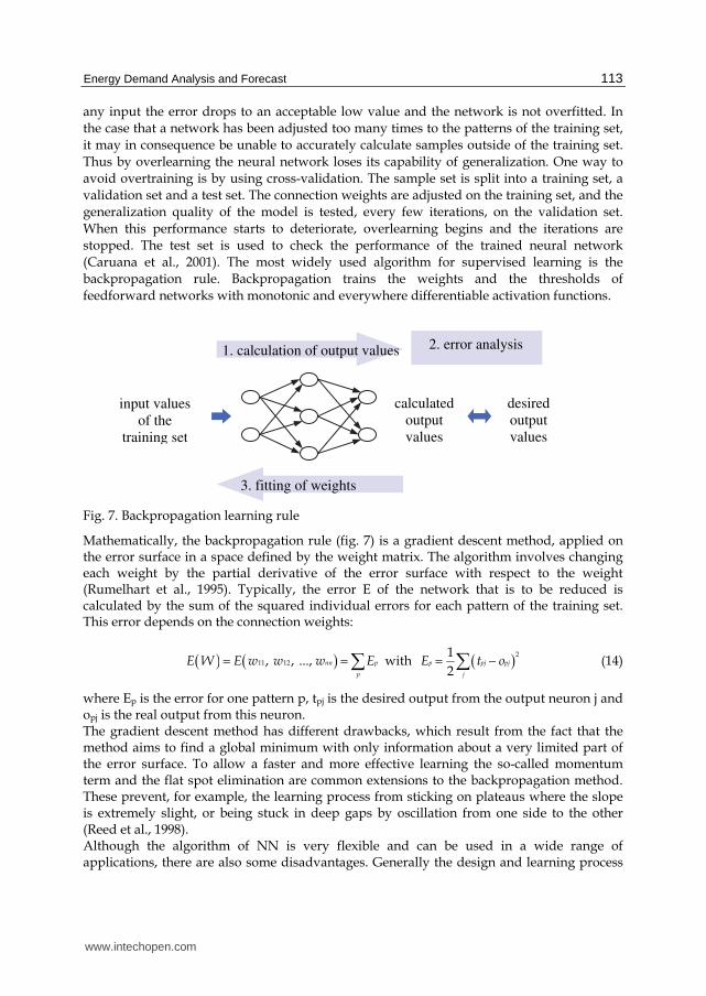
Fig. 6. Structure of a neuron
To calculate its new output depending on the input coming from the preceding units (or
from outside) a neuron uses three functions (Galushkin, 2007): First the inputs to the neuron
j from the preceding units combined with the connection weights are accumulated to yield
the net input. This value is subsequently transformed by the activation function fact, which
also takes into account the previous activation value and the threshold j (bias) of the
neuron to yield the new activation value of the neuron. The final output oj can be expressed
as a function of the new activation value of the neuron. In most of the cases this function fout
is not used so that the output of the neurons is identical to their activation values (fig. 6).
Three sigmoid (S-shaped) activation functions are usually applied: the logistic, hyperbolic
tangent and limited sine function. The formulas of the functions are given by:
log1
1 xf x
e tanh tanhx x
x x
e ef x x
e e
sin
1 for x 2
sin for 2 2
1 for x 2
f x x x
(13)
A neural network has to be configured such that the application of a set of inputs produces
the desired set of outputs. This is obtained by training, which involves modifying the
connection weights. In supervised learning methods, after initializing the weights to
random values, the error between the desired output and the actual output to a given input
vector is used to determine the weight changes in the net. During training, input pattern
after input pattern is presented to the network and weights are continually adapted until for
neuron
weighted
connection
weight of the
connection wiij
j
input layer
hidden layer
output layer
www.intechopen.com
Energy Demand Analysis and Forecast
113
any input the error drops to an acceptable low value and the network is not overfitted. In
the case that a network has been adjusted too many times to the patterns of the training set,
it may in consequence be unable to accurately calculate samples outside of the training set.
Thus by overlearning the neural network loses its capability of generalization. One way to
avoid overtraining is by using cross-validation. The sample set is split into a training set, a
validation set and a test set. The connection weights are adjusted on the training set, and the
generalization quality of the model is tested, every few iterations, on the validation set.
When this performance starts to deteriorate, overlearning begins and the iterations are
stopped. The test set is used to check the performance of the trained neural network
(Caruana et al., 2001). The most widely used algorithm for supervised learning is the
backpropagation rule. Backpropagation trains the weights and the thresholds of
feedforward networks with monotonic and everywhere differentiable activation functions.
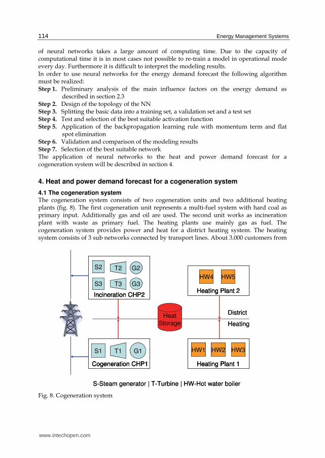
Fig. 7. Backpropagation learning rule
Mathematically, the backpropagation rule (fig. 7) is a gradient descent method, applied on the error surface in a space defined by the weight matrix. The algorithm involves changing each weight by the partial derivative of the error surface with respect to the weight (Rumelhart et al., 1995). Typically, the error E of the network that is to be reduced is calculated by the sum of the squared individual errors for each pattern of the training set. This error depends on the connection weights:
11 12, , ..., nn p
p
E W E w w w E with 21
2p pj pj
j
E t o (14)
where Ep is the error for one pattern p, tpj is the desired output from the output neuron j and opj is the real output from this neuron. The gradient descent method has different drawbacks, which result from the fact that the method aims to find a global minimum with only information about a very limited part of the error surface. To allow a faster and more effective learning the so-called momentum term and the flat spot elimination are common extensions to the backpropagation method. These prevent, for example, the learning process from sticking on plateaus where the slope is extremely slight, or being stuck in deep gaps by oscillation from one side to the other (Reed et al., 1998). Although the algorithm of NN is very flexible and can be used in a wide range of applications, there are also some disadvantages. Generally the design and learning process
calculated
output
values
desired
output
values
input values
of the
training set
1. calculation of output values 2. error analysis
3. fitting of weights
www.intechopen.com
Energy Management Systems
114
of neural networks takes a large amount of computing time. Due to the capacity of computational time it is in most cases not possible to re-train a model in operational mode every day. Furthermore it is difficult to interpret the modeling results. In order to use neural networks for the energy demand forecast the following algorithm must be realized: Step 1. Preliminary analysis of the main influence factors on the energy demand as
described in section 2.3 Step 2. Design of the topology of the NN Step 3. Splitting the basic data into a training set, a validation set and a test set Step 4. Test and selection of the best suitable activation function Step 5. Application of the backpropagation learning rule with momentum term and flat
spot elimination Step 6. Validation and comparison of the modeling results Step 7. Selection of the best suitable network The application of neural networks to the heat and power demand forecast for a cogeneration system will be described in section 4.
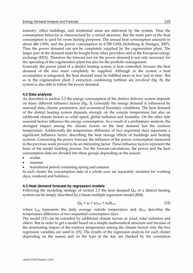
4. Heat and power demand forecast for a cogeneration system
4.1 The cogeneration system The cogeneration system consists of two cogeneration units and two additional heating plants (fig. 8). The first cogeneration unit represents a multi-fuel system with hard coal as primary input. Additionally gas and oil are used. The second unit works as incineration plant with waste as primary fuel. The heating plants use mainly gas as fuel. The cogeneration system provides power and heat for a district heating system. The heating system consists of 3 sub networks connected by transport lines. About 3.000 customers from
District
Heating
Cogeneration CHP1
T1 G1S1
Heat
Storage
Incineration CHP2
G2S2
T3
T2
S3 G3
HW1 HW2 HW3
Heating Plant 1
HW4 HW5
Heating Plant 2
S-Steam generator | T-Turbine | HW-Hot water boiler
District
Heating
Cogeneration CHP1
T1 G1S1
Cogeneration CHP1
T1 G1S1
Heat
Storage
Incineration CHP2
G2S2
T3
T2
S3 G3
Incineration CHP2
G2S2
T3
T2
S3 G3
HW1 HW2 HW3
Heating Plant 1
HW1 HW2 HW3
Heating Plant 1
HW4 HW5
Heating Plant 2
HW4 HW5
Heating Plant 2
S-Steam generator | T-Turbine | HW-Hot water boiler
Fig. 8. Cogeneration system
www.intechopen.com
Energy Demand Analysis and Forecast
115
industry, office buildings, and residential areas are delivered by the system. Thus the consumption behavior is characterized by a mixed structure. But the main part of the heat consumption is used for room heating purposes. The annual heat consumption amounts to about 460 GWh, and the power consumption to 6.700 GWh (Schellong & Hentges, 2007). Thus the power demand can not be completely supplied by the cogeneration plant. The larger part of the demand must be bought from other providers and at the European energy exchange (EEX). Therefore the forecast tool for the power demand is not only necessary for the operating of the cogeneration plant but also for the portfolio management. Generally the power plant of a district heating system is heat controlled, because the heat demand of the area must completely be supplied. Although in the system a heat accumulator is integrated, the heat demand must be fulfilled more or less 'just in time'. But as in the cogeneration plant 3 extraction condensing turbines are involved (fig. 8), the system is also able to follow the power demand.
4.2 Data analysis As described in section 2.3 the energy consumption of the district delivery system depends on many different influence factors (fig. 3). Generally the energy demand is influenced by seasonal data, climate parameters, and economical boundary conditions. The heat demand of the district heating system depends strongly on the outside temperature but also on additional climate factors as wind speed, global radiation and humidity. On the other side seasonal factors influence the energy consumption. As a result of a preliminary analysis, the strongest impact among the climate factors on the heat demand has the outdoor temperature. Additionally the temperature difference of two sequential days represents a significant influence factor, describing the heat storage effects of buildings and heating systems. Concerning the power forecast, the influence of the power consumption measured in the previous week proved to be an interesting factor. These influence factors represent the basis of the model building process. For the forecast calculations, the power and the heat consumption data are divided into three groups depending on the season:
winter
summer
transitional period containing spring and autumn In each cluster the consumption data of a whole year are separately modeled for working days, weekend and holidays.
4.3 Heat demand forecast by regression models Following the modeling strategy of section 2.3 the heat demand Qth of a district heating system can be simply described by a linear multiple regression model (RM):
Qth = a0 + a1tout + a2Δtout (15)
where tout represents the daily average outside temperature and Δtout describes the temperature difference of two sequential consumption days. The model (15) can be extended by additional climate factors as wind, solar radiation and others. But in order to get a model based on a simple mathematical structure and because of the dominating impact of the outdoor temperature among the climate factors only the two regression variables are used in (15). The results of the regression analysis for each cluster depending on the season and on the type of the day are checked by the correlation
www.intechopen.com

Energy Management Systems
116
coefficients and by a residual analysis. Corresponding to the modeling aspects described in chapter 2.2 for each season and each weekday a regression model (see equation 1) is calculated. The models describe the dependence of the daily heat demand on the outdoor temperature and the temperature difference of two sequential days. In order to estimate the regression parameters of the model (15) the database of the reference year is split up into the training set and the test set. The regression parameters are calculated by solving the corresponding least squares optimization (see section 3.4) on the basis of the training set. The quality of the model is checked by the comparison between the forecasted and the real heat consumption for the test dataset. The correlation coefficients and the mean prediction errors (see table 1) are used as quality parameter. The mean error is calculated for each model by:
1
| |1100%
nth real
reali
Q Q
n Q , where n represents the number of test data (16)
For the reference year the correlation coefficients range from 0.81 for the summer time to 0.93 for the winter season. The quality of the regression models of the heat consumption strongly depends on seasonal effects. The modeling results show that the quality of the models for the summer and transitional seasons is worse in comparison with the winter time (Schellong & Hentges, 2007). The large errors in the summer and transitional periods are caused by the fact that during the 'warmer' season the heat demand does not really depend on the outside temperature. In this case the heat is only needed for the hot water supply in the residential areas.
season summer transitional period winter
day type workdays weekend workdays weekend workdays weekend
16.0 12.0 12.9 19.8 5.5 5.6
Table 1. Mean errors for the daily heat demand forecast calculated by RM
4.4 Heat and power demand forecast by neural networks 4.4.1 Methodology In order to calculate the forecast of the heat and power demand, feedforward networks are used with one layer of hidden neurons connected to all neurons of the input and output layer. The applied learning rule is the backpropagation method with momentum term and flat spot elimination (see section 3.5). The optimal learning parameters are defined by testing different values and retaining the values which require the lowest number of training cycles. In order to find the most accurate model, several types of neural networks are trained and their prediction error for the test set is compared corresponding to formula (16). Networks with different numbers of hidden neurons are used with three sigmoid (S-shaped) activation functions: the logistic, hyperbolic tangent and limited sine function. Each neural net is trained three times up to the beginning overlearning phase and then the net with the best forecast is retained (Schellong & Hentges, 2011). Corresponding to the preliminary data analysis described in section 4.1 the power and the heat consumption data are divided into three groups depending on the season: winter, summer, and the transitional period. In each cluster the consumption data are separately
www.intechopen.com
Energy Demand Analysis and Forecast
117
modeled for working and for holidays. Thus overall 18 networks have to be tested for the heat and power demand models. For each network the topology varies from 3 to 8 neurons in the hidden layer. Following the mathematical modeling strategies of section 2.2 such models are preferred which have a simple structure. Thus overlearning effects can be avoided, and the adaptation properties of the model will be better than for more complex structures. Furthermore computing time can be reduced.
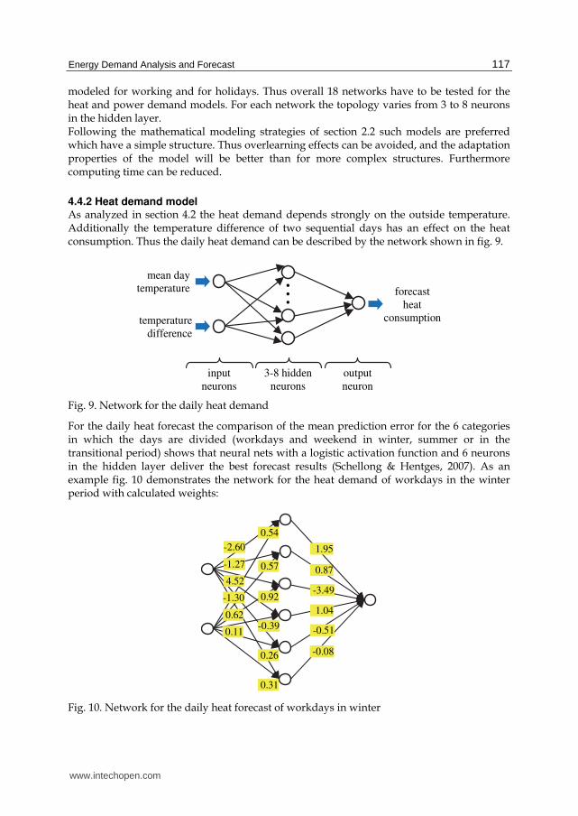
4.4.2 Heat demand model As analyzed in section 4.2 the heat demand depends strongly on the outside temperature. Additionally the temperature difference of two sequential days has an effect on the heat consumption. Thus the daily heat demand can be described by the network shown in fig. 9.
•• •
mean day
temperature
input
neurons
3-8 hidden
neurons
output
neuron
forecast
heat
consumptiontemperature
difference
Fig. 9. Network for the daily heat demand
For the daily heat forecast the comparison of the mean prediction error for the 6 categories in which the days are divided (workdays and weekend in winter, summer or in the transitional period) shows that neural nets with a logistic activation function and 6 neurons in the hidden layer deliver the best forecast results (Schellong & Hentges, 2007). As an example fig. 10 demonstrates the network for the heat demand of workdays in the winter period with calculated weights:
0.87
-3.49
1.04
-0.51
-0.08
4.52
-1.30
0.62
0.11
0.57
0.92
-0.39
0.26
0.31
-1.27
-2.60 1.95
0.54
Fig. 10. Network for the daily heat forecast of workdays in winter
www.intechopen.com
Energy Management Systems
118
Table 2 contains the mean prediction errors corresponding to formula (16). For the winter period we achieve the same quality of modeling results in comparison with RM (table 1).
season summer transitional period winter
day type workdays weekend workdays weekend workdays weekend
16.1 12.0 15.0 15.8 5.6 5.7
Table 2. Mean errors for the daily heat demand forecast calculated by NN
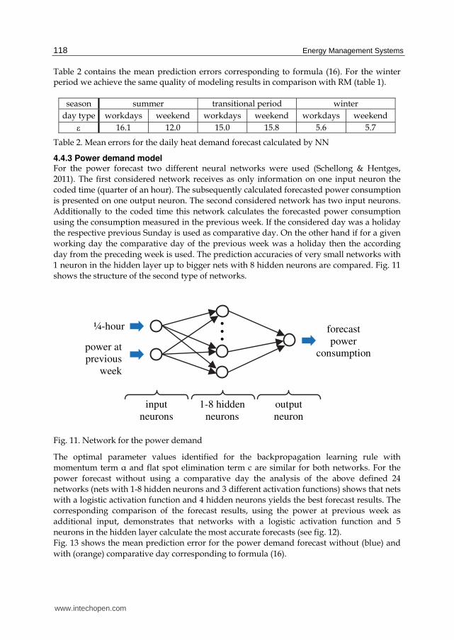
4.4.3 Power demand model For the power forecast two different neural networks were used (Schellong & Hentges,
2011). The first considered network receives as only information on one input neuron the
coded time (quarter of an hour). The subsequently calculated forecasted power consumption
is presented on one output neuron. The second considered network has two input neurons.
Additionally to the coded time this network calculates the forecasted power consumption
using the consumption measured in the previous week. If the considered day was a holiday
the respective previous Sunday is used as comparative day. On the other hand if for a given
working day the comparative day of the previous week was a holiday then the according
day from the preceding week is used. The prediction accuracies of very small networks with
1 neuron in the hidden layer up to bigger nets with 8 hidden neurons are compared. Fig. 11
shows the structure of the second type of networks.
•• •
¼-hour
power at
previous
week
input
neurons
1-8 hidden
neurons
output
neuron
forecast
power consumption
Fig. 11. Network for the power demand
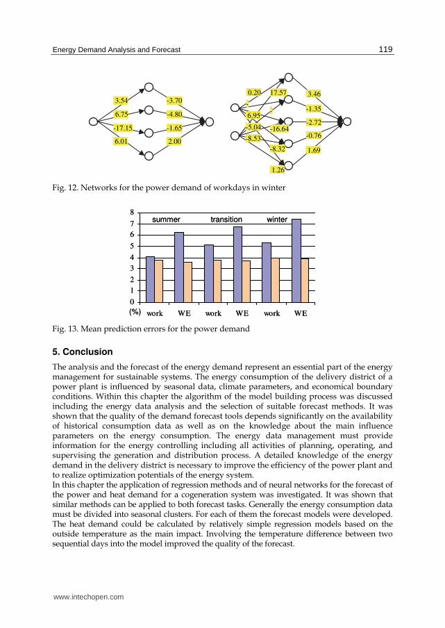
The optimal parameter values identified for the backpropagation learning rule with
momentum term α and flat spot elimination term c are similar for both networks. For the
power forecast without using a comparative day the analysis of the above defined 24
networks (nets with 1-8 hidden neurons and 3 different activation functions) shows that nets
with a logistic activation function and 4 hidden neurons yields the best forecast results. The
corresponding comparison of the forecast results, using the power at previous week as
additional input, demonstrates that networks with a logistic activation function and 5
neurons in the hidden layer calculate the most accurate forecasts (see fig. 12).
Fig. 13 shows the mean prediction error for the power demand forecast without (blue) and
with (orange) comparative day corresponding to formula (16).
www.intechopen.com
Energy Demand Analysis and Forecast
119
Fig. 12. Networks for the power demand of workdays in winter
0
1
2
3
4
5
6
7
8
work WE work WE work WE
summer transition winter
(%)
0
1
2
3
4
5
6
7
8
work WE work WE work WE
summer transition winter
(%)
Fig. 13. Mean prediction errors for the power demand
5. Conclusion
The analysis and the forecast of the energy demand represent an essential part of the energy management for sustainable systems. The energy consumption of the delivery district of a power plant is influenced by seasonal data, climate parameters, and economical boundary conditions. Within this chapter the algorithm of the model building process was discussed including the energy data analysis and the selection of suitable forecast methods. It was shown that the quality of the demand forecast tools depends significantly on the availability of historical consumption data as well as on the knowledge about the main influence parameters on the energy consumption. The energy data management must provide information for the energy controlling including all activities of planning, operating, and supervising the generation and distribution process. A detailed knowledge of the energy demand in the delivery district is necessary to improve the efficiency of the power plant and to realize optimization potentials of the energy system. In this chapter the application of regression methods and of neural networks for the forecast of the power and heat demand for a cogeneration system was investigated. It was shown that similar methods can be applied to both forecast tasks. Generally the energy consumption data must be divided into seasonal clusters. For each of them the forecast models were developed. The heat demand could be calculated by relatively simple regression models based on the outside temperature as the main impact. Involving the temperature difference between two sequential days into the model improved the quality of the forecast.
-3.70
-4.80
-1.65
2.00
3.54
6.75
-17.15
6.01
3.46
-1.35
-2.72
-0.76
1.69
0.20
-
6.95
-5.04
-8.53
17.57
-
-16.64
-8.32
1.26
www.intechopen.com

Energy Management Systems
120
Additionally feedforward networks were used with one layer of hidden neurons connected to all neurons of the input and output layer in order to calculate the forecast of the heat and power demand. The backpropagation method with momentum term and flat spot elimination was applied as learning rule. Neural networks using the coded time and the consumption measured in the previous week as inputs produced good forecast results for the power demand. Thus the quality of the power and heat forecast could be improved by using information of the 'near' past.
6. References
Box, G. & Jenkins, G. (1976). Time series analysis, forecasting and control. Prentice Hall, NY, USA, ISBN 0-130-60774-6
Caruana, R.; Lawrence, S. & Giles, C. (2001). Overfitting in Neural Nets: Backpropagation, Conjugate Gradient, and Early Stopping. Advances in Neural Information Processing Systems, Vol 13, MIT Press, Cambridge MA ,pp. 402-408, ISBN 100-262-12241-3
Deuflhard, P. & Hohmann, A. (2003). Numerical Analysis in Modern Scientific Computing. Springer Verlag, New York, ISBN 0-387-95410-4
Doty, S. & Turner, W, (2009). Energy management handbook. The Fairmont press, Inc., Lilburn, USA, ISBN 0-88173-609-0
Draper, N. & Smith, H. (1998). Applied Regression Analysis. Wiley Series in Probability and Statistics, New York, ISBN 0-471-17082-8
Fine, T. L (1999). Feedforward Neural Network Methodology. Springer Verlag, New York, ISBN 978-0-387-98745-3 Fischer, M. (2008). Modeling and Forecasting energy demand: Principles and difficulties, In
Management of Weather and Climate Risk in the Energy Industry, Troccoli, A. (Ed.), pp. 207-226, Springer Verlag, ISBN 978-90-481-3691-9, Dordrecht, The Netherlands.
Galushkin, A. (2007). Neural Networks Theory. Springer Verlag, New York, ISBN 978-3-540-48124-9 Hahn, H.; Meyer-Nieberg, S. & Pickl, S. (2009). Electric load forecasting methods: tools for
decision making. European Journal of Operational Research, Vol.199, No.3, pp. 902-907, ISSN 0377-2217
Maegaard, P. & Bassam, N. (2004). Integrated Renewable Energy for Rural Communities, Planning Guidelines, Technologies and Applications. Elsevier, ISBN 0-444-51014-1
Petchers, N. (2003). Combined heating, cooling and power handbook. The Fairmont press, Inc., Lilburn, USA, ISBN 0-88173-4624
Reed, R. & Marks, R. (1998). Neural Smithing: Supervised Learning in Feedforward Artificial Neural Networks. MIT Press, Cambridge MA, ISBN-10:0-262-18190-8
Rumelhart, D.; Durbin, R.; Golden, R. & Chauvin, Y. (1995). Backpropagation: The basic theory. In Backpropagation: Theory, architectures, and applications, Chauvin, Y. & Rumelhart, D. (Ed.), pp. 1-34., Lawrence Erlbaum, Hillsdale New Jersey, ISBN-10: 0805812598
Schellong, W. (2006). Integrated energy management in distributed systems. Proc. Conf. Power Electronics Electrical Drives, Automation and Motion, SPEEDAM 2006, pp. 492-496, ISBN 1-4244-0193-3 , Taormina, Italy, 2006
Schellong, W. & Hentges, F. (2007). Forecast of the heat demand of a district heating system. Proc. 7th Conf. on Power and Energy Systems, pp. 383-388, ISBN 978-0-88986-689-8, Palma de Mallorca, Spain, 2007
Schellong, W. & Hentges, F. (2011). Energy Demand Forecast for a Cogeneration System. Proc. 3rd Conf. on Clean Electrical Power, Ischia, Italy, 2011
VDEW (1999). Standard load profiles. VDEW Frankfurt (Main), Germany
www.intechopen.com

Energy Management SystemsEdited by Dr Giridhar Kini
ISBN 978-953-307-579-2Hard cover, 274 pagesPublisher InTechPublished online 01, August, 2011Published in print edition August, 2011
InTech EuropeUniversity Campus STeP Ri Slavka Krautzeka 83/A 51000 Rijeka, Croatia Phone: +385 (51) 770 447 Fax: +385 (51) 686 166www.intechopen.com
InTech ChinaUnit 405, Office Block, Hotel Equatorial Shanghai No.65, Yan An Road (West), Shanghai, 200040, China
Phone: +86-21-62489820 Fax: +86-21-62489821
This book comprises of 13 chapters and is written by experts from industries, and academics from countriessuch as USA, Canada, Germany, India, Australia, Spain, Italy, Japan, Slovenia, Malaysia, Mexico, etc. Thisbook covers many important aspects of energy management, forecasting, optimization methods and theirapplications in selected industrial, residential, generation system. This book also captures important aspects ofsmart grid and photovoltaic system. Some of the key features of books are as follows: Energy managementmethodology in industrial plant with a case study; Online energy system optimization modelling; Energyoptimization case study; Energy demand analysis and forecast; Energy management in intelligent buildings;PV array energy yield case study of Slovenia;Optimal design of cooling water systems; Supercapacitor designmethodology for transportation; Locomotive tractive energy resources management; Smart grid and dynamicpower management.
How to referenceIn order to correctly reference this scholarly work, feel free to copy and paste the following:
Wolfgang Schellong (2011). Energy Demand Analysis and Forecast, Energy Management Systems, DrGiridhar Kini (Ed.), ISBN: 978-953-307-579-2, InTech, Available from:http://www.intechopen.com/books/energy-management-systems/energy-demand-analysis-and-forecast

© 2011 The Author(s). Licensee IntechOpen. This chapter is distributedunder the terms of the Creative Commons Attribution-NonCommercial-ShareAlike-3.0 License, which permits use, distribution and reproduction fornon-commercial purposes, provided the original is properly cited andderivative works building on this content are distributed under the samelicense.
Recommended