Empirics for Economic Growth and Convergence
by
Danny T. Quah�
LSE Economics Department and CEP
CENTRE FOR ECONOMIC PERFORMANCE
DISCUSSION PAPER NO. 253
July 1995
This paper is produced as part of the Centre's Programme on National Economic
Performance.
� Comments by J. Dolado, F. Giavazzi, and an anonymous referee have been
important in re-shaping this article. X. Sala-i-Martin has generously donated
insight and time to try and make me understand. He need not, however, agree with
all my statements below. All calculations were performed using the econometrics
shell tsrf.
Nontechnical Summary
The convergence hypothesis|that poor economies might \catch up"|
has generated a huge empirical literature: this paper critically reviews
some of the earlier key �ndings, clari�es their implications, and relates
them to more recent results. Particular attention is devoted to interpret-
ing convergence empirics. The paper argues that relating them to growth
theories, as usually done, gives but one interpretation to convergence dy-
namics; it does not exhaust their importance. Instead, if we relate con-
vergence to the dynamics of income distributions, it broadens the issues
on which such empirics can shed light; it connects with policy concerns
on persistent or growing inequality, regional core-periphery stagnation,
and tendencies for ongoing capital ows across developed and developing
countries. The main �ndings are: (1) The much-heralded uniform 2% rate
of convergence could arise for reasons unrelated to the dynamics of eco-
nomic growth. (2) Usual empirical analyses|cross-section (conditional)
convergence regressions, time series modelling, panel data analysis|can
be misleading for understanding convergence; a model of polarization in
economic growth clari�es those di�culties. (3) The data, more reveal-
ingly modelled, show persistence and immobility across countries: some
evidence supports Baumol's idea of \convergence clubs"; some evidence
shows the poor getting poorer, and the rich richer, with the middle class
vanishing. (4) Convergence, unambiguous up to sampling error, is ob-
served across US states.
Empirics for Economic Growth and Convergence
by
Danny T. Quah
LSE Economics Department and CEP
November 1995
ABSTRACT
The convergence hypothesis has generated a huge empirical literature:
this paper critically reviews some of the earlier key �ndings, clari�es their
implications, and relates them to more recent results. Particular atten-
tion is devoted to interpreting convergence empirics. The main �ndings
are: (1) The much-heralded uniform 2% rate of convergence could arise
for reasons unrelated to the dynamics of economic growth. (2) Usual
empirical analyses|cross-section (conditional) convergence regressions,
time series modelling, panel data analysis|can be misleading for under-
standing convergence; a model of polarization in economic growth clari�es
those di�culties. (3) The data, more revealingly modelled, show persis-
tence and immobility across countries: some evidence supports Baumol's
idea of \convergence clubs"; some evidence shows the poor getting poorer,
and the rich richer, with the middle class vanishing. (4) Convergence, un-
ambiguous up to sampling error, is observed across US states.
Keywords: evolving distributions, Galton's fallacy, polarization, regional dynam-
ics, stochastic kernel, unit root
JEL Classi�cation: C21, C22, C23, O41
Communications to: D. T. Quah, LSE, Houghton Street, London WC2A 2AE.
[Tel: +44-171-955-7535, Fax: +44-171-831-1840, Email: [email protected]]

1. Introduction
It �res the imagination that policy might be able to in uence economic growth,
thereby allowing poor economies [countries, regions, states, provinces, districts,
cities, : : : ] either to catch up with those already richer, or to languish, depending.
This intellectual excitement is reminiscent of how macroeconomists used to view
their ability to stabilize business cycles.
Standard neoclassical models assumed growth to be an inexorable, exogenous
process; little then could be said on how growth comes about. More recent the-
ories allow growth to be an endogenous outcome: this, in part, explains renewed
interest in long-run macroeconomic behavior, and motivates a research program
for empirically discriminating between these two kinds of models in the real world.
Over-simplifying drastically, a convenient way to distinguish the two views on
growth is to ask, \Are poor economies incipiently catching up with those already
richer? Or, instead, are they caught in a poverty trap?" Many caveats would be
needed for such an evaluation to be proper, but that catch-up could occur has
come to be known as the convergence hypothesis. What is important, though, is
that such a hypothesis bears independent interest in economics.
Di�erent kinds of economic convergence are routinely discussed and widely
debated. Examples include convergence in incomes between rich and poor parts of
the European Union; in plant and �rm size in industries; in economic activity across
di�erent regions (states, provinces, districts, or cities) within the same country;
in asset returns and in ation rates across countries in a common trade area; in
political attitudes across di�erent groups; in wages across industries, professions,
and geographical regions.
These examples show that convergence is simply a basic empirical issue, one
that re ects on|among other things|polarization, income distribution, and in-
equality. Certainly, understanding economic growth is important. But growth is
only one of many di�erent areas in economics where analyzing convergence sheds
useful insight.1
1 Recent applications of convergence-related insights, outside economic growth,
{ 2 {
Recent studies on per capita income convergence claim to have uncovered
a profound empirical regularity. Poor and rich economies|across di�erent geo-
graphical disaggregations; across regions within di�erent countries; across di�er-
ent administrative units; over di�erent time samples|all appear to be converging
towards each other at a stable, uniform rate of 2% per year. This uniformity is
striking, and has been used to pronounce on matters as diverse as German reuni�-
cation; the e�ects of regional redistribution within individual countries and across
the European Union; and the increasing income inequality within countries while
the opposite (allegedly) takes place across countries. This paper parallels [35] in
reviewing empirical �ndings on convergence. However, our emphases, interpreta-
tions, and criticisms di�er su�ciently that the two papers overlap little.
Section 2 begins the analysis by asking if the 2% convergence-rate unifor-
mity might arise for reasons irrelevant to growth models. The idea here is that
such consistency might only re ect something mechanical and independent of the
economic structure of growth. The working hypothesis, then, is that economic
structure varies in many|explicable and inexplicable|ways across environments,
and thus cannot be the source for the 2% uniformity. Instead, that uniformity is
due to something relatively uninteresting, namely, the statistical implications of
a unit root in the time series data. Section 2 examines how far such \mechani-
cal" econometric-based explanations can go in explaining conventional empirical
�ndings on convergence. The answer is that they go part of the way, but not all.
Section 3 turns to interpreting convergence dynamics. Here, interest lies partly
in the claim that those dynamics shed light on the validity of di�erent growth mod-
els. But more direct, and perhaps more important, is the claim that convergence
would show the poor catching up with the rich. (This is a growth issue, sure,
but not exclusively so.) Does conventional evidence on convergence shed light on
include [12, 13, 19, 20, 28, 31]. Such empirical issues predate [14, 17, 27], by close to
a century, formal endogenous growth models. By coincidence these issues appeared
in the industrial organization literature at about the same time as Solow's original
growth analysis; see [17] and references.
{ 3 {
this? Section 3 argues that the answer is no: reasons range from Galton's fallacy
to researchers' confusing \average" and cross-distribution dynamics. To illustrate
further, section 4 presents a growth model whose key observable implications are
completely disguised in typical convergence regressions. Whether such a model
shows convergence or divergence is a semantic subtlety; this is not normally trou-
bling. In scienti�c work, mathematical symbols make the intent precise enough.
However, most empirical discussions of convergence do not.
Section 5 describes the results from using alternative, more revealing empir-
ics to analyze income data across countries and states. The �rst key �nding is
that \convergence clubs" [4, 6] are found at the top and bottom of the income
distribution across countries: the rich are becoming richer; the poor, poorer; with
the middle-class vanishing. The second key �nding is that in some|although not
all|samples the usual convergence conclusions hold. However, they do so for rea-
sons that are not revealed by those models that are typical in this literature (e.g.,
all those in [35]). This is for reasons described in Sections 3 and 4: those standard
models generate empirics ill-suited for comparison with the dynamics of a rich
cross section of data. Section 6 brie y concludes.
2. Earlier empirical evidence
Sala-i-Martin [35] compactly summarizes and extends the recent conventional ev-
idence on growth and convergence.2 He emphasizes regional dynamics, but the
methodological and theoretical discussions apply readily to aggregate economies.
Thus this section's di�cult work is already done. I simply highlight here some key
points in [35] before providing my own critical evaluation of this research.
Integral to these discussions are the concepts of �- and �-convergence [1].
The striking discovery is the cross-sample stability of rates of �-convergence. A
wide range of examples over di�erent time spans|US states, Japanese prefectures,
and di�erent regional European groupings|shows this regularity. The empirical
2 In this section I assume some basic familiarity with what is known as �-
convergence in this literature; the next section makes things precise.
{ 4 {
fact|that convergence occurs, and does so at the rate of 2% per annum|comes
shining through again and again. Such stability is spectacular and profound, in a
profession where very little empirical remains invariant to close scrutiny.
But by the same token one should be skeptical of such �ndings. How much
can one believe growth to be the same across economies, provided only that a
few obvious, measurable heterogeneities are removed? And that, further, in that
growth process (after conditioning), economies are converging towards the same,
unique long-run growth path? Put another way, how credible is it that the simple
conditioning used in this literature removes all signi�cant di�erences in economic
growth across economies, so that countries are converging? If not, then why does
such apparent uniformity obtain?
Thus, this section critically examines if the 2% estimate in �-convergence
regressions could arise from a structure completely unrelated to the economics of
growth. Finding it so would undermine the claim that that uniformity re ects an
interesting economic mechanism.3
To understand the discussion that follows, recall the usual derivation of the
convergence regression equation. Expositions of this abound, so I need only refer
the reader to one of the clearest: equations (1){(8) in [2]. Equation (8) there is
taken to be the important observable implication of the neoclassical growth model.
This prediction can be written:
T�1 (Yj(T )� Yj(0)) = a�
�1� e��T
T
�Yj(0) + uj(T ); (2:1)
where I use Y to denote log per capita income, and keep only essential details.
Interpret the right hand side of (2.1) as average or long-run growth rate, and
3 The referee has suggested an alternative \mechanical" explanation involving
the log/nonlinear transformations used in �-convergence regressions. Suggestive
computer simulations supporting that conjecture were also generously provided by
that referee. I have, however, been unable to provide an analytical explanation for
those simulations, whereas I can for mine below.
{ 5 {
� as the rate of convergence. The term u is a residual tacked on the end for
regression analysis; it is assumed to be uncorrelated with appropriate right-hand
side explanatory variables. Thus, equation (2.1) hypothesizes that the average
growth rate depends on|among other things|the initial condition Yj(0).
Estimating equation (2.1) by nonlinear least squares, averaging across j in a
cross-section|regions, states, countries|constitutes the canonical �-convergence
analysis. An investigator sometimes also groups the time-series observations into
blocks of T periods each: panel data methods are then applied to equation (2.1),
averaging across both time and cross section. Occasionally, when time series ob-
servations have su�cient length, a series of equations (2.1) might be estimated,
one for each j: in this case, the investigator averages only across time.
The empirical results in [1, 2, 3, 35] and elsewhere show a remarkable cluster-
ing of � estimates around a central tendency. That tendency is the magic 2% rate
of convergence. The magic modi�er emphasizes this same value's arising from such
diverse geographical and time samples. Perhaps it really is the case that the under-
lying economic structure across countries and regions is invariant. The stability
of this 2%-rate would then call for explanation, likely along the lines suggested
in [35]. Alternatively, it might be that underlying structures truly di�er across
time and space, but that enough of a uniformity exists to produce this stability.
The question is, Is that uniformity related to convergence dynamics in economic
growth?
Recall that a uniformity|well-known in time series econometrics|is borne
by unit root stochastic processes.4 Fix a time series X = fX(t) : t � 0g. While
its underlying structure can be quite heterogeneous, as long as it carries a (unit
root) stochastic trend, then all other features are eventually subservient to that
stochastic trend. I admit this language is a little colorful; it is my interpretation
of the following.
4 Unit root time series e�ects are investigated for economic growth and conver-
gence also in [7, 8], although there for di�erent purposes than in this section.
{ 6 {
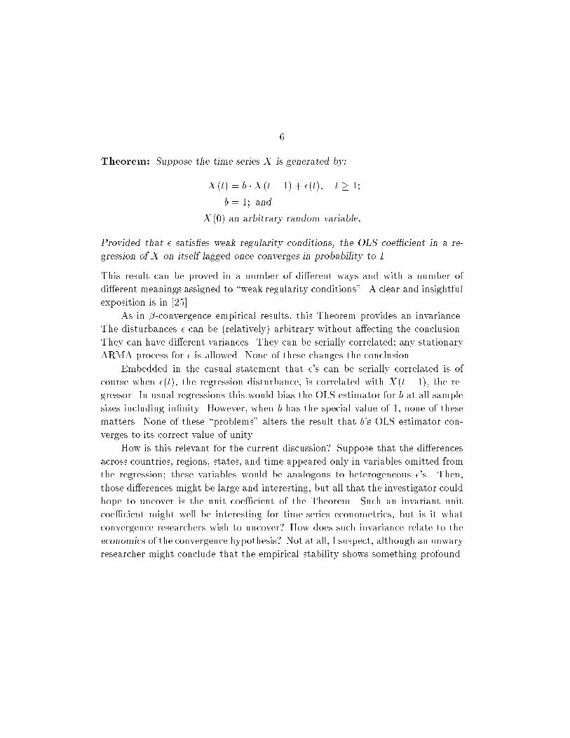
Theorem: Suppose the time series X is generated by:
X(t) = b �X(t� 1) + �(t); t � 1;
b = 1; and
X(0) an arbitrary random variable:
Provided that � satis�es weak regularity conditions, the OLS coe�cient in a re-
gression of X on itself lagged once converges in probability to 1.
This result can be proved in a number of di�erent ways and with a number of
di�erent meanings assigned to \weak regularity conditions". A clear and insightful
exposition is in [25].
As in �-convergence empirical results, this Theorem provides an invariance.
The disturbances � can be (relatively) arbitrary without a�ecting the conclusion.
They can have di�erent variances. They can be serially correlated; any stationary
ARMA process for � is allowed. None of these changes the conclusion.
Embedded in the casual statement that �'s can be serially correlated is of
course when �(t), the regression disturbance, is correlated with X(t� 1), the re-
gressor. In usual regressions this would bias the OLS estimator for b at all sample
sizes including in�nity. However, when b has the special value of 1, none of these
matters. None of these \problems" alters the result that b's OLS estimator con-
verges to its correct value of unity.
How is this relevant for the current discussion? Suppose that the di�erences
across countries, regions, states, and time appeared only in variables omitted from
the regression; these variables would be analogous to heterogeneous �'s. Then,
those di�erences might be large and interesting, but all that the investigator could
hope to uncover is the unit coe�cient of the Theorem. Such an invariant unit
coe�cient might well be interesting for time-series econometrics, but is it what
convergence researchers wish to uncover? How does such invariance relate to the
economics of the convergence hypothesis? Not at all, I suspect, although an unwary
researcher might conclude that the empirical stability shows something profound.
{ 7 {
Is it merely idle speculation that connects the Theorem's invariance with the
stability of � in convergence regressions? After all, those regressions aren't exactly
the regressions described by the Theorem. But, then again, how di�erent are they?
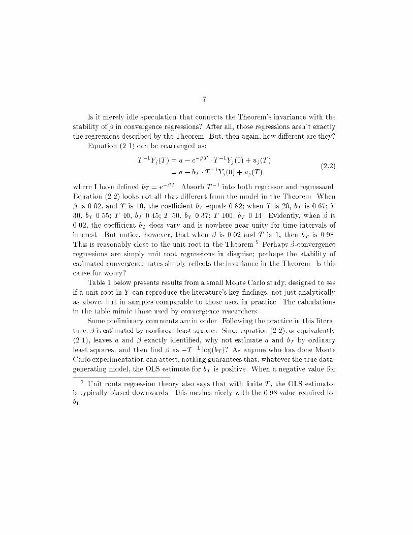
Equation (2.1) can be rearranged as:
T�1Yj(T ) = a + e��T � T�1Yj(0) + uj(T )
= a + bT � T�1Yj(0) + uj(T );
(2:2)
where I have de�ned bT = e��T . Absorb T�1 into both regressor and regressand.
Equation (2.2) looks not all that di�erent from the model in the Theorem. When
� is 0.02, and T is 10, the coe�cient bT equals 0.82; when T is 20, bT is 0.67; T
30, bT 0.55; T 40, bT 0.45; T 50, bT 0.37; T 100, bT 0.14. Evidently, when � is
0.02, the coe�cient bT does vary and is nowhere near unity for time intervals of
interest. But notice, however, that when � is 0.02 and T is 1, then bT is 0.98.
This is reasonably close to the unit root in the Theorem.5 Perhaps �-convergence
regressions are simply unit-root regressions in disguise; perhaps the stability of
estimated convergence rates simply re ects the invariance in the Theorem. Is this
cause for worry?
Table 1 below presents results from a small Monte Carlo study, designed to see
if a unit root in Y can reproduce the literature's key �ndings, not just analytically
as above, but in samples comparable to those used in practice. The calculations
in the table mimic those used by convergence researchers.
Some preliminary comments are in order. Following the practice in this litera-
ture, � is estimated by nonlinear least squares. Since equation (2.2), or equivalently
(2.1), leaves a and � exactly identi�ed, why not estimate a and bT by ordinary
least squares, and then �nd � as �T�1 log(bT )? As anyone who has done Monte
Carlo experimentation can attest, nothing guarantees that, whatever the true data-
generating model, the OLS estimate for bT is positive. When a negative value for
5 Unit roots regression theory also says that with �nite T , the OLS estimator
is typically biased downwards|this meshes nicely with the 0.98 value required for
b1.
{ 8 {
bT occurs, � is unde�ned. Estimating � by nonlinear least squares in the form of
either equations (2.2) or (2.1) rescues the investigator from this embarrassment.
Doing so, however, introduces a di�erent problem: when the best-�tting bTis negative or zero, any good nonlinear least squares program will try to give �
a value of in�nity. Thus in �nite samples very large positive values for � can
be generated in Monte Carlo draws, thereby pulling rightward the estimator's
simulated distribution. This then gives Monte Carlo averages for convergence rates
that are even faster than 2%|even when the true data-generating model comprises
cross-sectionally independent random walks, and thus shows no convergence.6
To remove this bias in my favor (since the immediate assignment is to cast
doubt on convergence �ndings), I have trimmed the Monte Carlo distributions for
b-estimators at machine accuracy for the exponential function.7 Table 1 presents
results for a variety of time-series lengths T and cross-section sizes N . Each column
block, under a given value of T , contains three numbers for each value of N . The
�rst number is the average � in the trimmed Monte Carlo distribution; how close
this is to 2% shows how well the conjectures above hold up. The second number
(in parentheses) is the cross-Monte Carlo sample standard deviation (not the esti-
mated standard error from nonlinear estimation): this is the appropriate notion of
imprecision in our experiment. Finally, the third number [in brackets] denotes the
fraction of draws rejected in trimming the Monte Carlo distribution; this number
is smaller for larger N and T , re ecting our estimator's convergence in probability
to the correct, well-de�ned parameter value.8 The true data-generating process in
6 Of course, this problem goes away as the sample gets arbitrarily large, but for
that we already have the analytical results above. It is precisely the small-sample
case that we currently need to consider.7 Thus, my tsrf program generating the table will produce slightly di�erent
results across di�erent machines. The NeXT that I use probably has slightly
better accuracy than most other personal computers.8 Large N , large T analysis can be found in, e.g., [29]. The convergence in
probability here follows easily from that analysis.
{ 9 {
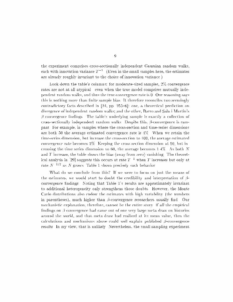
the experiment comprises cross-sectionally independent Gaussian random walks,
each with innovation variance T�1. (Even in the small samples here, the estimates
are already roughly invariant to the choice of innovation variance.)
Look down the table's columns: for moderate-sized samples, 2% convergence
rates are not at all atypical|even when the true model comprises mutually inde-
pendent random walks, and thus the true convergence rate is 0. Our reasoning says
this is nothing more than �nite-sample bias. It therefore reconciles two seemingly
contradictory facts described in [24, pp. 255{6]: one, a theoretical prediction on
divergence of independent random walks; and the other, Barro and Sala-i-Martin's
�-convergence �ndings. The table's underlying sample is exactly a collection of
cross-sectionally independent random walks. Despite this, �-convergence is ram-
pant. For example, in samples where the cross-section and time-series dimensions
are both 50 the average estimated convergence rate is 4%. When we retain the
time-series dimension, but increase the cross-section to 100, the average estimated
convergence rate becomes 2%. Keeping the cross-section dimension at 50, but in-
creasing the time-series dimension to 60, the average becomes 1.4%. As both N
and T increase, the table shows the bias (away from zero) vanishing. The theoret-
ical analysis in [29] suggests this occurs at rate T�1 when T increases but only at
rate N�1=2 as N grows. Table 1 shows precisely such behavior.
What do we conclude from this? If we were to focus on just the means of
the estimates, we would start to doubt the credibility and interpretation of �-
convergence �ndings. Noting that Table 1's results are approximately invariant
to additional heterogeneity only strengthens those doubts. However, the Monte
Carlo distributions also endow the estimates with high variability (the numbers
in parentheses), much higher than �-convergence researchers usually �nd. Our
mechanistic explanation, therefore, cannot be the entire story. If all the empirical
�ndings on �-convergence had came out of one very large meta-draw on histories
around the world, and that meta-draw had realized at its mean value, then the
calculations and mechanisms above could well explain published �-convergence
results. In my view, that is unlikely. Nevertheless, the small sampling experiment
{ 10 {
does suggest that part of the explanation could be merely a statistical invariance|
interesting from the viewpoint of econometric theory, less so from the perspective
of economic convergence.
3. Convergence predictions in growth theory
Many studies of convergence empirics still share the same theoretical motivation
as that given in [2]. Recall how dynamics are analyzed there: one log-linearizes
the deterministic Cass-Koopmans model about steady state, and then notices that
the growth rate of output per worker depends on the log deviation from steady
state.
This dependence is parameterized, as usual, by a negative eigenvalue of a �rst-
derivatives matrix. In the model that eigenvalue varies with the ratio of physical
capital's marginal to average product, or equivalently, when factor markets are
competitive, physical capital's factor share in income. The larger is that ratio or
factor share, the closer is the relevant eigenvalue to zero, and thus, the slower is
the rate of convergence.
Barro and Sala-i-Martin's [1, 2] estimated �-convergence rate implies cap-
ital factor shares larger than the 0.4 given in national income accounts. The
same convergence estimate also says physical capital enters the production func-
tion importantly (has marginal product that doesn't diminish quickly; see, e.g.,
[34]). In this analysis the two|estimated convergence rates and physical capital's
compensation|together create a puzzle for neoclassical growth theory. For some
economists, it is this and only this that justi�es interest in convergence empirics.
Others will quickly disagree|even before questioning the accuracy of the es-
timated numbers. Most obvious, if the researcher's interest lies only in the coef-
�cients of a production function, then why not just estimate those directly? A
long and revered tradition in empirical analysis|associated with [16] and many
others|treats exactly that estimation problem. Starting from there, and re�ning
estimates, would appear sensible if one were interested in parameters in a produc-
tion function. Using the dynamics of state, regional, or cross-country data only
{ 11 {
to make a point about a coe�cient in a Cobb-Douglas production function (say)
seems circuitous, although creative.
More tenable might be to recall the independent interest in convergence:
whether poorer economies are incipiently catching up with richer ones is a ba-
sic question, and of considerable interest. Relating the question to the parameters
of a neoclassical production function merely places an interpretation on it; it does
not exhaust its importance. Answering this broader convergence question would
directly address issues raised in [4]. It would speak to the concerns of European
Commission policy-makers analyzing inequality (divergence) across European re-
gions [5]. Finally, addressing the question this way brings into the (macroeco-
nomic) analysis ideas and insights from the economics of income distributions.9
The coupling of the convergence hypothesis to these broader issues is, arguably,
what animates debate here|more than does concern with just the parameters of
an aggregate production function.
The discussion that follows will be easier to understand if one keeps in mind
these broader issues. Doing so immediately clari�es the usefulness of di�erent
concepts of convergence.10 To begin, recall Barro and Sala-i-Martin's [1, 2] �- and
�-convergence.
Roughly put, �-convergence is when in a cross-section regression of (time-
averaged) growth rates on initial levels, the coe�cient on initial levels is negative:
\poorer regions grow faster." Conditional �-convergence is again a negative coef-
�cient, but only when that regression has the appropriate, additional explanatory
9 Distinguish this, however, from work such as [15]. That work focuses on the
relation between aggregate growth and the distribution of income across people
within an economy. Here, instead, I refer to using income distribution ideas to
model dynamics across many economies.10 One shouldn't really need to say this here (except that misunderstandings
should be corrected earlier rather than later): the issues here di�er from the usual
probabilist's distinction between convergence in probability, in law, almost sure,
in Lp, and so on.
{ 12 {
variables on the right hand side. While potentially important in practice, for the
discussion here the di�erence between conditional and unconditional convergence
adds no conceptual insight. Thus, I will not mention conditional convergence fur-
ther in this section; in the next I raise it, but only to indicate how it confuses
issues.
Again, roughly put, �-convergence is when the dispersion of cross-section
levels diminishes over time. Typically, dispersion is measured by sample standard
deviation. Here, it is irrelevant whether a single country shows convergence (in
mean square) to steady state or to anything else: what matters, instead, is how
the entire cross-section behaves.
The literature (e.g., [1, 35]) has already explored some of the relation between
�- and �-convergence. Here, I give precise de�nitions, and study the connection
more fully; this will also help motivate the dynamically evolving distribution em-
pirics to be given below.
Let Yj(t) denote|as above|the log of economy j's income at time t. Say
that the data
Y = fYj(t) : j = 1; 2; : : : ; N ; t = 0; 1; : : : ; Tg
show �-convergence if for all t the cross-section projection
P (Yj(t)� Yj(0)jYj(0))def= (bt � 1)� Yj(0); (3:1)
has
bt � 1 < 0:
Let �t denote the (N -sample-size) cross-section standard deviation, i.e.,
�t =
�N�1
NXj=1
�Yj(t)�
�N�1
NXk=1
Yk(t)
��2�1=2
; (3:2)
and say that data Y show �-convergence if �t � �t�1 for all t. Some might
insist on �t ! 0 as t grows large but that will never be observable, and so is
{ 13 {
not a useful criterion in practice. Also, the inequality is weak rather than strict to
allow situations where �t has already converged, i.e., the cross-section is already in
(stochastic) steady state. Even when �t is unchanging through time, the economies
underlying the cross section could still be moving about within that invariant
distribution: this is, after all, what \stochastic steady state" means.
Current interest lies only in the relation between di�erent concepts of conver-
gence. Thus, sampling variability is inessential in the discussion; I will ignore it in
manipulating (3.1) and (3.2).
Begin with an extreme special case. Suppose Y 's are independent and identi-
cally distributed (iid) cross-sectionally, and in time follow:
Yj(t) = bYj(t� 1) + uj(t); jbj < 1;
Yj(0) independent of uj(t); t � 1;(3:3)
where u is iid also in time, and has positive, �nite variance �2u. (That Y has been
assumed iid across j implies u iid across j.)
Equation (3.3) implies that
�2t = b2�2t�1 + �2u =) limt!1
�2t = (1� b2)�1�2u
and
bt = bt =) bt � 1 < 0 for all t:
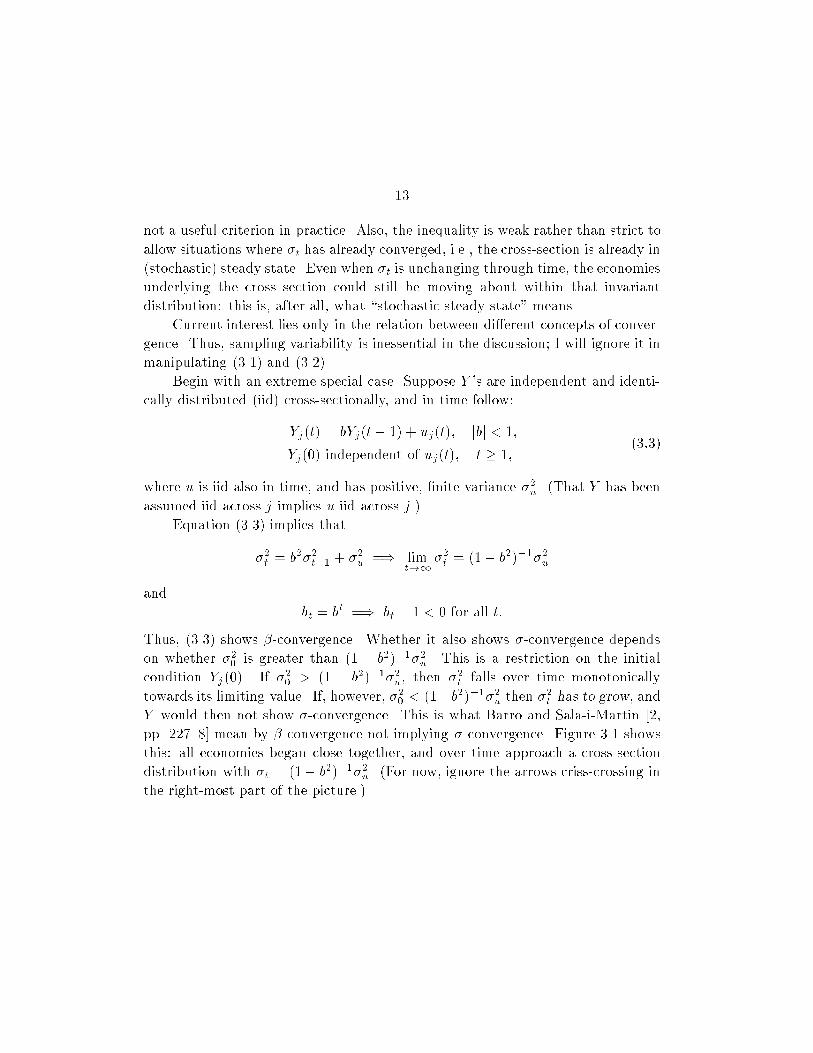
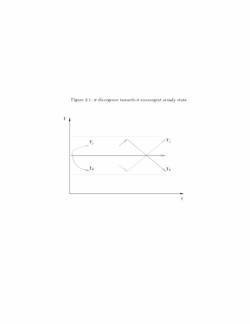
Thus, (3.3) shows �-convergence. Whether it also shows �-convergence depends
on whether �20 is greater than (1 � b2)�1�2u. This is a restriction on the initial
condition Yj(0). If �20 > (1 � b2)�1�2u, then �2t falls over time monotonically
towards its limiting value. If, however, �20 < (1�b2)�1�2u then �2t has to grow, and
Y would then not show �-convergence. This is what Barro and Sala-i-Martin [2,
pp. 227{8] mean by �-convergence not implying �-convergence. Figure 3.1 shows
this: all economies began close together, and over time approach a cross-section
distribution with �t = (1� b2)�1�2u. (For now, ignore the arrows criss-crossing in
the right-most part of the picture.)
{ 14 {
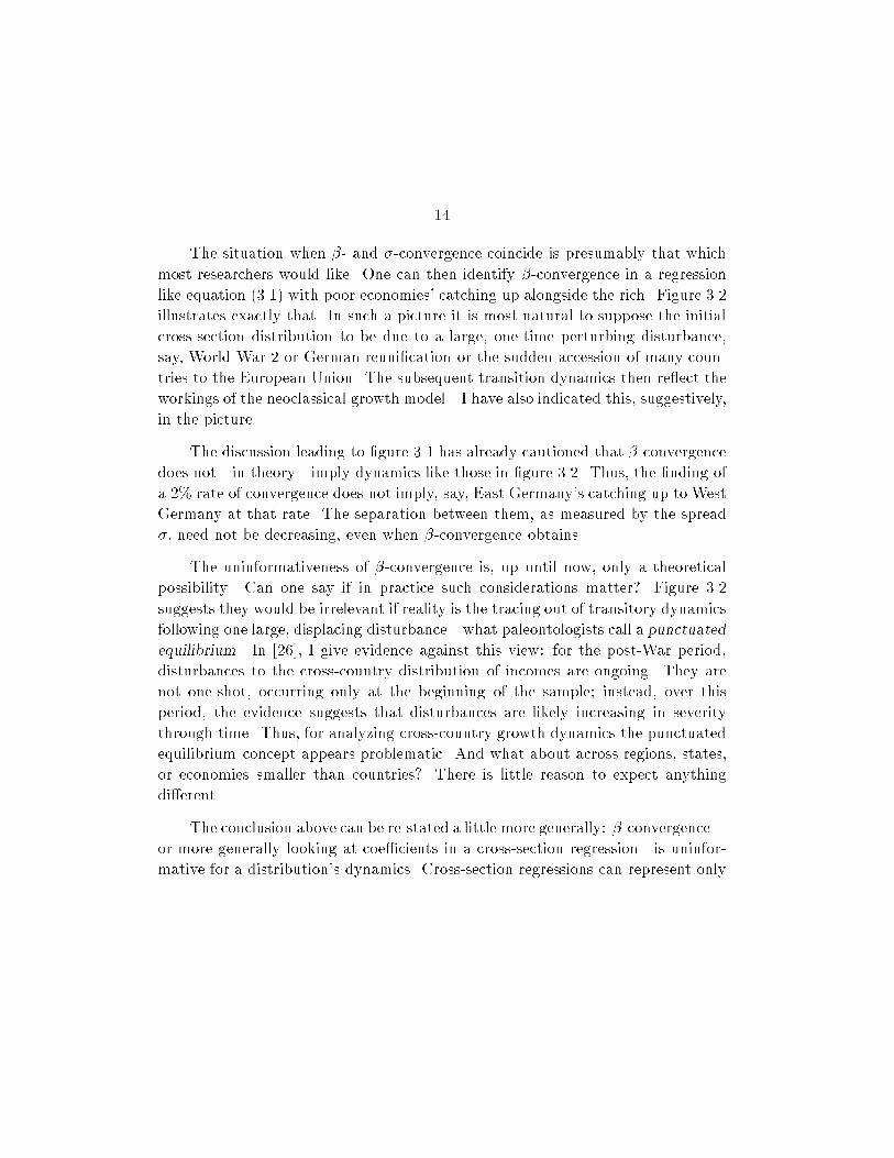
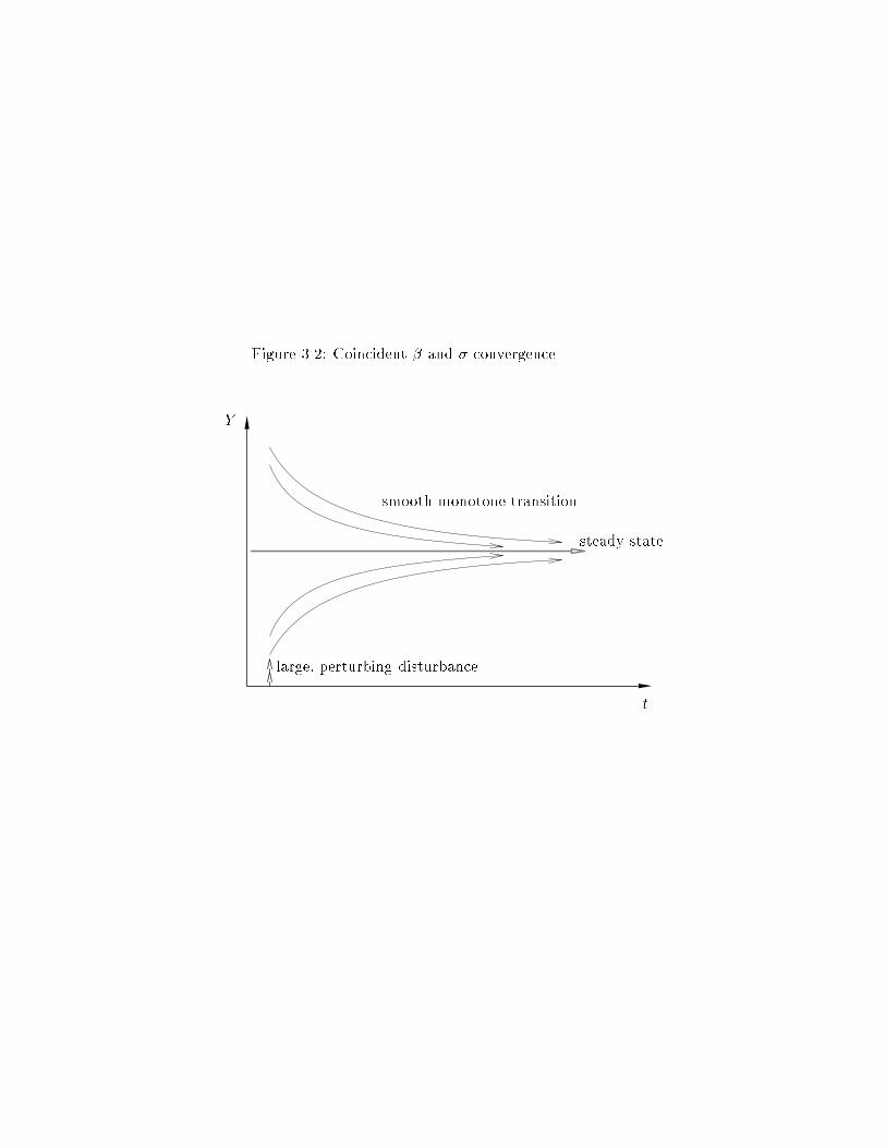
The situation when �- and �-convergence coincide is presumably that which
most researchers would like. One can then identify �-convergence in a regression
like equation (3.1) with poor economies' catching up alongside the rich. Figure 3.2
illustrates exactly that. In such a picture it is most natural to suppose the initial
cross-section distribution to be due to a large, one-time perturbing disturbance,
say, World War 2 or German reuni�cation or the sudden accession of many coun-
tries to the European Union. The subsequent transition dynamics then re ect the
workings of the neoclassical growth model|I have also indicated this, suggestively,
in the picture.
The discussion leading to �gure 3.1 has already cautioned that �-convergence
does not|in theory|imply dynamics like those in �gure 3.2. Thus, the �nding of
a 2% rate of convergence does not imply, say, East Germany's catching up to West
Germany at that rate. The separation between them, as measured by the spread
�, need not be decreasing, even when �-convergence obtains.
The uninformativeness of �-convergence is, up until now, only a theoretical
possibility. Can one say if in practice such considerations matter? Figure 3.2
suggests they would be irrelevant if reality is the tracing out of transitory dynamics
following one large, displacing disturbance|what paleontologists call a punctuated
equilibrium. In [26], I give evidence against this view: for the post-War period,
disturbances to the cross-country distribution of incomes are ongoing. They are
not one-shot, occurring only at the beginning of the sample; instead, over this
period, the evidence suggests that disturbances are likely increasing in severity
through time. Thus, for analyzing cross-country growth dynamics the punctuated
equilibrium concept appears problematic. And what about across regions, states,
or economies smaller than countries? There is little reason to expect anything
di�erent.
The conclusion above can be re-stated a little more generally: �-convergence|
or more generally looking at coe�cients in a cross-section regression|is uninfor-
mative for a distribution's dynamics. Cross-section regressions can represent only
{ 15 {
average behavior, not the behavior of an entire distribution.11
Going over the reasoning above, a reader might conclude that looking at �-
convergence would get around all these di�culties. Whether �-convergence implies
�-convergence or not then becomes irrelevant: the focus will have moved to �-
convergence directly. This, obviously, solves the previously-mentioned problems.
But it introduces new subtleties.
From observations already noted above, disturbances to the cross section of
economies should be viewed as ongoing over time. If so, then one is not going to
see �t tending to zero, but at best to a positive constant. Go to that limit: the
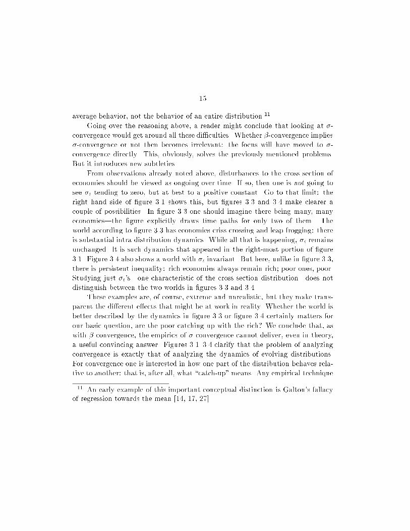
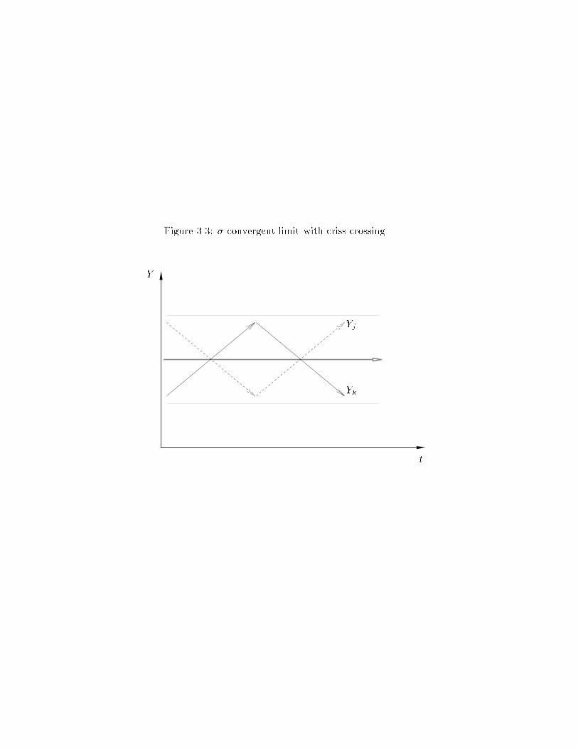
right hand side of �gure 3.1 shows this, but �gures 3.3 and 3.4 make clearer a
couple of possibilities. In �gure 3.3 one should imagine there being many, many
economies|the �gure explicitly draws time paths for only two of them. The
world according to �gure 3.3 has economies criss-crossing and leap-frogging: there
is substantial intra-distribution dynamics. While all that is happening, �t remains
unchanged. It is such dynamics that appeared in the right-most portion of �gure
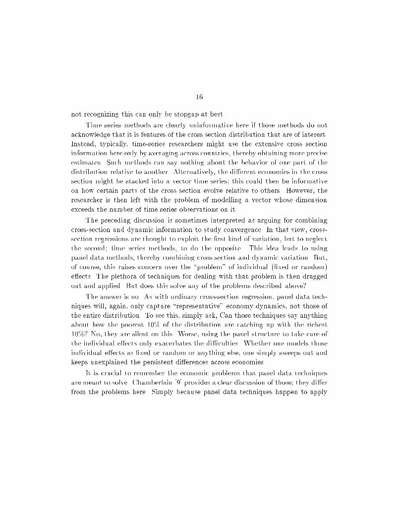
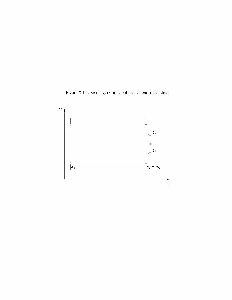
3.1. Figure 3.4 also shows a world with �t invariant. But here, unlike in �gure 3.3,
there is persistent inequality: rich economies always remain rich; poor ones, poor.
Studying just �t's|one characteristic of the cross section distribution|does not
distinguish between the two worlds in �gures 3.3 and 3.4.
These examples are, of course, extreme and unrealistic, but they make trans-
parent the di�erent e�ects that might be at work in reality. Whether the world is
better described by the dynamics in �gure 3.3 or �gure 3.4 certainly matters for
our basic question, are the poor catching up with the rich? We conclude that, as
with �-convergence, the empirics of �-convergence cannot deliver, even in theory,
a useful convincing answer. Figures 3.1{3.4 clarify that the problem of analyzing
convergence is exactly that of analyzing the dynamics of evolving distributions.
For convergence one is interested in how one part of the distribution behaves rela-
tive to another: that is, after all, what \catch-up" means. Any empirical technique
11 An early example of this important conceptual distinction is Galton's fallacy
of regression towards the mean [14, 17, 27].
{ 16 {
not recognizing this can only be stopgap at best.
Time series methods are clearly uninformative here if those methods do not
acknowledge that it is features of the cross section distribution that are of interest.
Instead, typically, time-series researchers might use the extensive cross section
information here only by averaging across countries, thereby obtaining more precise
estimates. Such methods can say nothing about the behavior of one part of the
distribution relative to another. Alternatively, the di�erent economies in the cross
section might be stacked into a vector time series; this could then be informative
on how certain parts of the cross section evolve relative to others. However, the
researcher is then left with the problem of modelling a vector whose dimension
exceeds the number of time series observations on it.
The preceding discussion is sometimes interpreted as arguing for combining
cross-section and dynamic information to study convergence. In that view, cross-
section regressions are thought to exploit the �rst kind of variation, but to neglect
the second; time series methods, to do the opposite. This idea leads to using
panel data methods, thereby combining cross section and dynamic variation. But,
of course, this raises concern over the \problem" of individual (�xed or random)
e�ects. The plethora of techniques for dealing with that problem is then dragged
out and applied. But does this solve any of the problems described above?
The answer is no. As with ordinary cross-section regression, panel data tech-
niques will, again, only capture \representative" economy dynamics, not those of
the entire distribution. To see this, simply ask, Can those techniques say anything
about how the poorest 10% of the distribution are catching up with the richest
10%? No, they are silent on this. Worse, using the panel structure to take care of
the individual e�ects only exacerbates the di�culties. Whether one models those
individual e�ects as �xed or random or anything else, one simply sweeps out and
keeps unexplained the persistent di�erences across economies.
It is crucial to remember the economic problems that panel data techniques
are meant to solve. Chamberlain [9] provides a clear discussion of those; they di�er
from the problems here. Simply because panel data techniques happen to apply
{ 17 {
to data with extensive cross-section and time-series variation does not mean they
are at once similarly appropriate for analyzing convergence.
4. An economic model: Conditional and unconditional convergence
The preceding analysis drew some pretty pictures. It then suggested that the
dynamics in those pictures cast doubt on the informativeness of standard growth
regressions. But is there an economic structure that could produce such dynamics?
This section describes a model that does so.
It is standard in many growth analyses to study how one economy, in isolation
from all other economies, grows quickly or slowly.12 The insights developed are
then used to explain why some countries grow faster than others.
The point made in the previous section bears on this and, with hindsight, is
obvious: studying an average or representative economy gives little insight into the
empirical behavior of the entire cross section. For such cross section dynamics to
be interpretable, one needs a theoretical model that makes predictions on them.
The model here draws from [30]. It makes predictions on cross section dynam-
ics by linking three observations: (i) countries endogenously select themselves into
groups, and thus do not act in isolation; (ii) specialization in production allows
exploiting economies of scale; and (iii) ideas are an important engine of growth.
The key results are two: (a) coalitions|or, as it will turn out, convergence
clubs|form endogenously; the model delivers predictions on coalition membership
across the entire cross section of economies; (b) di�erent convergence dynamics are
generated, depending on the initial distribution of characteristics across countries.
Included among these potential dynamics are explicit convergence club character-
izations; polarization|the rich becoming richer, the poor poorer, and the middle
class vanishing; strati�cation|multiple modes in the income distribution across
countries; and overtaking and divergence|two economies initially on roughly equal
footing, separating over time so that one eventually becomes wealthier than the
other.
12 Exceptions do exist, e.g., [18, 21].
{ 18 {
In [30] I show that coalitions, in equilibrium, are typically nondegenerate,
nontrivial subsets of the entire cross section of economies. The con�guration of
coalitions comes from recognizing the forces across countries for consolidation and
fragmentation. Equilibrium balances these opposing forces, and permits (at least
for a time) diversity. Coalitions can then be recognized as \convergence clubs,"
thereby determining international patterns of growth, convergence, and polariza-
tion.
The resulting dynamics are in general subtle, but special cases can be graph-
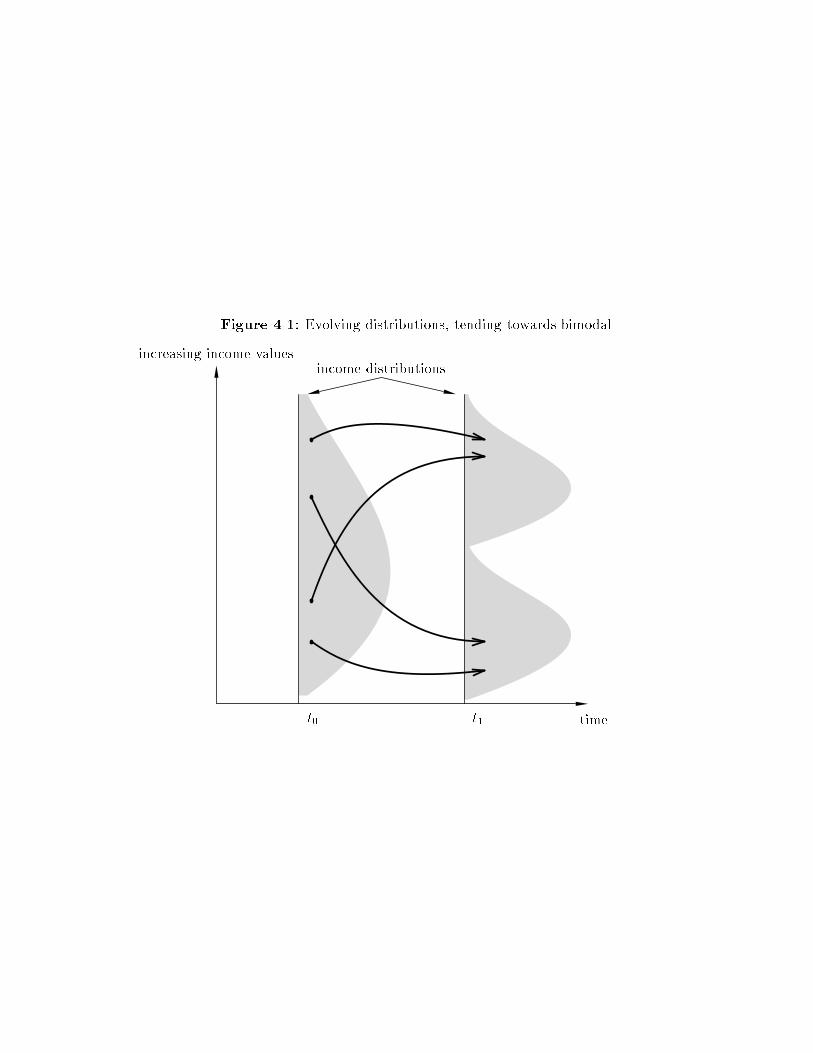
ically represented. Figure 4.1 shows some equilibrium time paths for incomes
(discounted by the steady-state growth rate).
In this example, at time t0 there is some initial income distribution across the
cross section of economies. Over time, some economies become better o�, others
worse o�; overtaking is possible. Coalitions or convergence clubs form, however,
and the distribution tends towards a bimodal distribution at time t1. In general,
the number of modal points equals the number of coalitions that form. When more
than two coalitions form, strati�cation is an apposite term in place of polarization
to describe the outcome. With two coalitions (as in �gure 4.1), the distribution
dynamics can be easily seen. Eventually, the middle-income group of economies
vanish, and the rich continue to become richer, and the poor, poorer. Clustering
occurs at high and low parts of the income distribution.
The exact outcome|the number of coalitions, their composition, and so on|
depends on the initial distribution of income across the entire cross section. If the
world began with all incomes already close together, then only a single coalition
forms; all countries then converge to equality. If, on the other hand, initial incomes
are disparate, then, more likely, multiple convergence clubs form. The distribution
dynamics will then be the multi-mode or strati�cation extension of �gure 4.1.
Economists observing these dynamics are naturally led to describe the resulting
groups as convergence clubs.
But what happens if researchers apply the tools of �-convergence analysis
to data generated by �gure 4.1? A researcher might attempt to understand the
{ 19 {
behavior of incomes across the cross section of economies by, say, \controlling"
for di�ering human capital stocks and other observable variables. That researcher
could then conclude that conditional convergence occurs, and that human capital
explains cross-country patterns of growth. However, such conclusions mislead.
It is, instead, the pattern of club membership that explains everything. In the
model, human capital is only responding endogenously to coalition structures:
that is why high human capital is found among rich-club countries. Moreover,
conditional convergence is not a useful way to think about the polarization induced
by convergence-club formations: the interesting strati�cation in �gure 4.1 is never
revealed by conditional-convergence investigations.
The dynamics in �gure 4.1 would be one motivation for the empirics devel-
oped in [11]. There, Durlauf and Johnson provide an innovative technique for
consistently uncovering local basins of convergence|they do this by allowing their
�tted regression model to \adapt" subsamples, depending on the data realizations
themselves. What I give below is a di�erent empirical method, but one that seems
to me more natural for studying evolving distributions. Durlauf and Johnson in-
terpret their empirics in terms of multiple regimes. I interpret �gure 4.1 as just one
equilibrium law of motion, but in an entire distribution, which could then have
multiple modal points in the ergodic limit. In general, each technique|that in
[11] and the section below|has advantages in di�erent dimensions over the other;
neither strictly dominates.
Finally, the empirical message here is not con�ned to this particular model of
ideas and growth. In [33] I adapted the model in [15] to produce much the same
empirical results as in �gure 4.1. Other models employing local nonconvexities in
the technology, nonlinearity in the savings function, and so on will, again, give the
same empirics (see, e.g., [6]).
{ 20 {
5. Revealing empirics
The analysis above has argued that standard convergence empirics are uninfor-
mative. This section describes some newer empirical results that overcome those
de�ciencies.
From �gure 4.1 it is obvious that the natural way to study convergence empir-
ics is to provide an empirical model for how distributions evolve.13 Let Ft denote
the distribution of incomes across countries at time t. Associated with such a dis-
tribution is a measure �t. The simplest model for the evolution of fFt : integer tg,
or equivalently f�t : integer tg, is an autoregression in measures:
8 measurable sets A : �t+1(A) =
ZM(y; A) d�t(y); (5:1)
where M is a stochastic kernel, mapping the Cartesian product of income values
and measurable sets to the interval [0; 1]. The kernel M maps one measure �t into
another �t+1, and tracks where in Ft+1 points in Ft end up. Thus, M encodes
information on intra-distribution dynamics, whether economies like Korea and the
Philippines, say, which were close together in 1950 transit subsequently to widely
di�erent income levels. It therefore contains strictly more information than just
aggregate statistics such as means or standard deviations.
Equation (5.1) is analogous to a standard time-series �rst-order vector au-
toregression, except its values are distributions (rather than scalars or vectors of
numbers), and it contains no explicit disturbance or innovation. By analogy with
autoregression, there is no reason why the law of motion in �t need be �rst order,
or why the relation need be time-invariant. Nevertheless, (5.1) is a useful �rst step
for analyzing dynamics in f�tg. Rewrite (5.1) as the convolution
�t+1 = M � �t: (5:2)
13 The ideas that follow were �rst stated in a simpler form in [26]. More precise
technical statements can be found in [30, 32].
{ 21 {
Iterating (5.2) yields (a predictor for) future cross section distributions
�t+s = (M �M � � � � �M) � �t = Ms� �t;
taking this to the limit as s ! 1, one can characterize the likely long-run or er-
godic distribution of cross-country incomes. Convergence towards equality might
manifest in f�t+sg tending towards a degenerate point measure; the world polar-
izing in the long run as in �gure 4.1 might manifest in f�t+sg tending towards a
two-point or bimodal measure. The speed of convergence of the evolving distri-
butions and their cross-sectional mobility properties can be studied from certain
spectral characteristics of the kernel M . Variants of (5.1) thus allow answering a
wealth of interesting questions about cross-sectional income dynamics.
How does one estimate something like M? The most natural �rst step is to
discretize the measures �t. Thereupon, M becomes just a transition probabil-
ity matrix; and �'s become nonnegative vectors on the unit simplex. Of course,
discretization distorts the underlying model; in Markov process theory, it is well
known that a �rst-order Markov process need no longer be even Markov when
inappropriately discretized. However, one suspects that for e�ects such as those
in �gure 4.1 the distortions will not conceal the important features.
Quah [26, 27] has calculated discretized estimates of M for the world's cross-
country distribution of per capita incomes. Table 2 reproduces one such result
from [26]. Taking each country's per capita GDP relative to the world average,
discretize the set of possible values into intervals at 1=4, 1=2, 1, and 2. All relevant
properties of M are then described by a 5� 5 transition matrix whose (j; k) entry
is the probability that an economy in income group j transits to income group k.
Low-numbered states correspond to low incomes; thus, for example, income group
1 (the �rst row and column) in table 2 comprises per capita incomes no greater
than one-fourth the world's average.
In table 2 the column labeled (Number) gives the total number of transitions
that have starting points in that income group. For example, the second row shows
that over the entire sample|across 118 countries and 23 years|643 observations
{ 22 {
fell in income group 2, i.e., started with incomes between one-fourth and one-
half the world average. Of these, 92% remained in that same income group the
following period.
Table 2 presents kernel M where the transition period is one year. The pre-
dominant feature is|not surprisingly|high persistence: all diagonal entries ex-
ceed 90%; other entries are non-zero only for the �rst state o� the main diagonal.
More interesting, however, is the �nal row, which tabulates the ergodic distribu-
tion implied by the estimated kernel.14 That distribution shows �rst, a thinning in
the middle, and second, an accumulation in both low and high tails. But these are
exactly the important features suggested in �gure 4.1: it is polarization that occurs
across the world, not convergence. Convergence clubs exist at the high and low
ends of the income distribution; the middle class is vanishing. (These tendencies
are also suggested informally by �gure 6 of [27, p. 436].)
Table 3 presents the same calculations, but now for US states. Here, much
greater mobility is apparent: diagonal entries are smaller; o�-diagonals, larger.
The evidence therefore suggests greater convergence occurring within the states
of the US. Also, note the ergodic distribution: it no longer shows the bimodal-
ity in rich and poor that is evident in world income distribution dynamics. No
convergence clubs or clusters are evident here.
In other papers [26, 27, 28, 32, 33] I have studied variations on the basic theme
here, namely, that empirical analysis of convergence is more revealing when it
provides information on how the entire distribution evolves|not just the dynamics
of a representative economy.15 Included among these variations are: allowing
higher-order dynamics than �rst-order as in equation (5.1); taking natural time
horizons to be greater than one year; allowing the grid-points in tables 2 and 3 to
adapt and evolve over time; not discretizing, but instead retaining the continuous
14 Nothing in the calculations enforces existence or uniqueness of an ergodic
distribution. It is a consequence of the data that precisely one such distribution
was found.15 Other subsequent, recent work following up on these ideas include [10, 22, 23].
{ 23 {
set of income values (in which case the kernelM becomes in�nite-dimensional, and
is estimated nonparametrically); permitting conditioning information; structuring
M so that it can be more easily interpreted. None of these alters the principal
�nding on polarization for the world cross-country distribution of incomes.
6. Conclusion
This paper has provided theoretical and empirical frameworks for studying con-
vergence. In doing so, it has overcome some di�culties in the traditional analysis
of, e.g., [2, 35].
The �rst point the paper made is that it is possible, although not likely,
that standard convergence �ndings are due to an uninteresting (from the current
perspective) statistical uniformity. But then, second, the paper provided a rich
array of examples to argue that those convergence �ndings might be misleading.
Next, the paper described a theoretical model of ideas and economic growth.
In the model, convergence clubs endogenously form, and the distribution of income
across economies polarizes. Rich economies become richer; poor ones, poorer; and
the middle class vanishes. Such a model produces equilibrium dynamics where
conventional empirical methods are problematic. The model suggests, instead,
alternative empirics based on studying the dynamics of evolving distributions.
The paper then gave results from such empirical analyses, suggesting the
strength of cross-country polarization present in the world. The paper argued
that that kind of divergence actually dominates the evidence on 2% convergence,
previously accepted as conventional wisdom.
References
[1] Barro, Robert J. and Sala-i-Martin, Xavier. (1991), \Convergence Across
States and Regions", Brookings Papers on Economic Activity, 1:107{182,
April.
[2] Barro, Robert J. and Sala-i-Martin, Xavier. (1992), \Convergence", Journal
of Political Economy, 100(2):223{251, April.
[3] Barro, Robert J. and Sala-i-Martin, Xavier. (1992), \Regional Growth and
Migration: A Japan-United States Comparison", Journal of the Japanese and
International Economies, 6(4):312{346, December.
[4] Baumol, William J., Blackman, Sue Anne Batey, and Wol�, Edward N. (1989),
Productivity and American Leadership: The Long View, MIT Press, Cam-
bridge MA 02139.
[5] Begg, Iain and Mayes, David. (1993), \Cohesion in the European Commu-
nity", Regional Science and Urban Economics, 23:427{448.
[6] Ben-David, Dan. (1994), \Convergence Clubs and Diverging Economies",
Working Paper 922, CEPR, London W1X 1LB, February.
[7] Bernard, Andrew B. and Durlauf, Steven N. (1993), \Interpreting Tests of
the Convergence Hypothesis", Working paper, MIT Economics Department,
December.
[8] Bernard, Andrew B. and Durlauf, Steven N. (1994), \Convergence in Inter-
national Output", Working paper, MIT Economics Department, February.
[9] Chamberlain, Gary. (1984), \Panel Data", in Griliches, Zvi and Intriligator,
Michael D., (eds.), Handbook of Econometrics vol. II, chapter 22, pages 1247{
1318. Elsevier North-Holland, Amsterdam.
[10] Desdoigts, Alain. Changes in the World Income Distribution: A Non-
Parametric Approach to Challenge the Neoclassical Convergence Argument.
PhD thesis, European University Institute, Florence, June 1994.
[11] Durlauf, Steven N. and Johnson, Paul. (1994), \Multiple Regimes and Cross-
Country Growth Behavior", Working paper, University of Wisconsin, May.
[12] Eckstein, Zvi and Eaton, Jonathan. (1994), \Cities and Growth: Theory and
Evidence from France and Japan", Working paper, Economics Department,
Tel-aviv University, September.
[13] Esteban, Joan-Mar��a and Ray, Debraj. (1994), \On the Measurement of Po-
larization", Econometrica, 62(4):819{851, July.
[14] Friedman, Milton. (1992), \Do Old Fallacies Ever Die?", Journal of Economic
Literature, 30(4):2129{2132, December.
[15] Galor, Oded and Zeira, Joseph. (1993), \Income Distribution and Macroeco-
nomics", Review of Economic Studies, 60(1):35{52, January.
[16] Griliches, Zvi and Ringstad, Vidar. (1971), Economies of Scale and the Form
of the Production Function, North-Holland, Amsterdam.
[17] Hart, Peter E. (1994), \Galtonian Regression Across Countries and the Con-
vergence of Productivity", Discussion Paper 19, University of Reading, March.
[18] Helpman, Elhanan. (1993), \Innovation, Imitation, and Intellectual Property
Rights", Econometrica, 61(6):1247{1280, November.
[19] Konings, Joep. Gross Job Flows and Wage Determination in the UK: Evidence
from Firm-Level Data. PhD thesis, LSE, London, July 1994.
[20] Koopmans, Reinout and Lamo, Ana R. (1994), \Cross-Sectional Firm Dy-
namics: Theory and Empirical Results from the Chemical Sector", Working
paper, Economics Department, LSE, London, April.
[21] Krugman, Paul. (1979), \AModel of Innovation, Technology Transfer, and the
World Distribution of Income", Journal of Political Economy, 87(2):253{266,
April.
[22] Lamo, Ana R. (tba). PhD thesis, LSE, London, 1995. in progress.
[23] Larch, Martin. (1994), \Regional Cross-Section Growth Dynamics in the
European Community", Working paper, European Institute, LSE, London,
June.
[24] Lucas Jr., Robert E. (1993), \Making a Miracle", Econometrica, 61(2):251{
271, March.
[25] Phillips, Peter C. B. (1987), \Time Series Regression with Unit Roots",
Econometrica, 55(2):277{302, March.
[26] Quah, Danny. (1993), \Empirical Cross-Section Dynamics in Economic
Growth", European Economic Review, 37(2/3):426{434, April.
[27] Quah, Danny. (1993), \Galton's Fallacy and Tests of the Convergence Hy-
pothesis", The Scandinavian Journal of Economics, 95(4):427{443, December.
[28] Quah, Danny. (1994), \Convergence across Europe", Working paper, Eco-
nomics Department, LSE, London, June.
[29] Quah, Danny. (1994), \Exploiting Cross Section Variation for Unit Root
Inference in Dynamic Data", Economics Letters, 44(1):9{19, January.
[30] Quah, Danny. (1994), \Ideas Determining Convergence Clubs", Working pa-
per, Economics Department, LSE, London, September.
[31] Quah, Danny. (1994), \One Business Cycle and One Trend from (Many,)
Many Disaggregates", European Economic Review, 38(3/4):605{613, April.
[32] Quah, Danny. (1995), \International Patterns of Growth: II. Persistence, Path
Dependence, and Sustained Take-o� in Growth Transition", Working paper,
LSE, January.
[33] Quah, Danny. (1996), \Convergence Empirics Across Economies with (Some)
Capital Mobility", Journal of Economic Growth. forthcoming.
[34] Romer, Paul M. (1994), \The Origins of Endogenous Growth", Journal of
Economic Perspectives, 8(1):3{22, Winter.
[35] Sala-i-Martin, Xavier. (1995), \Regional Cohesion: Evidence and Theories of
Regional Growth and Convergence", European Economic Review. forthcom-
ing.
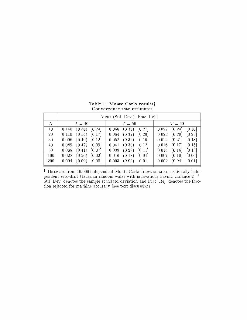
Table 1: Monte Carlo resultsyConvergence rate estimates
Mean (Std. Dev.) [Frac. Rej.]
N T = 40 T = 50 T = 60
10 0.140 (0.58) [0.24] 0.066 (0.38) [0.27] 0.027 (0.24) [0.30]
20 0.119 (0.54) [0.17] 0.064 (0.37) [0.20] 0.023 (0.20) [0.23]
30 0.096 (0.49) [0.12] 0.052 (0.32) [0.16] 0.024 (0.21) [0.18]
40 0.089 (0.47) [0.09] 0.041 (0.30) [0.12] 0.016 (0.17) [0.15]
50 0.068 (0.41) [0.07] 0.039 (0.28) [0.11] 0.014 (0.16) [0.13]
100 0.028 (0.26) [0.02] 0.016 (0.18) [0.04] 0.007 (0.10) [0.06]
200 0.004 (0.09) [0.00] 0.003 (0.06) [0.01] 0.002 (0.04) [0.01]
y These are from 10,000 independent Monte Carlo draws on cross-sectionally inde-pendent zero-drift Gaussian random walks with innovations having variance T�1.Std. Dev. denotes the sample standard deviation and Frac. Rej. denotes the frac-tion rejected for machine accuracy (see text discussion).
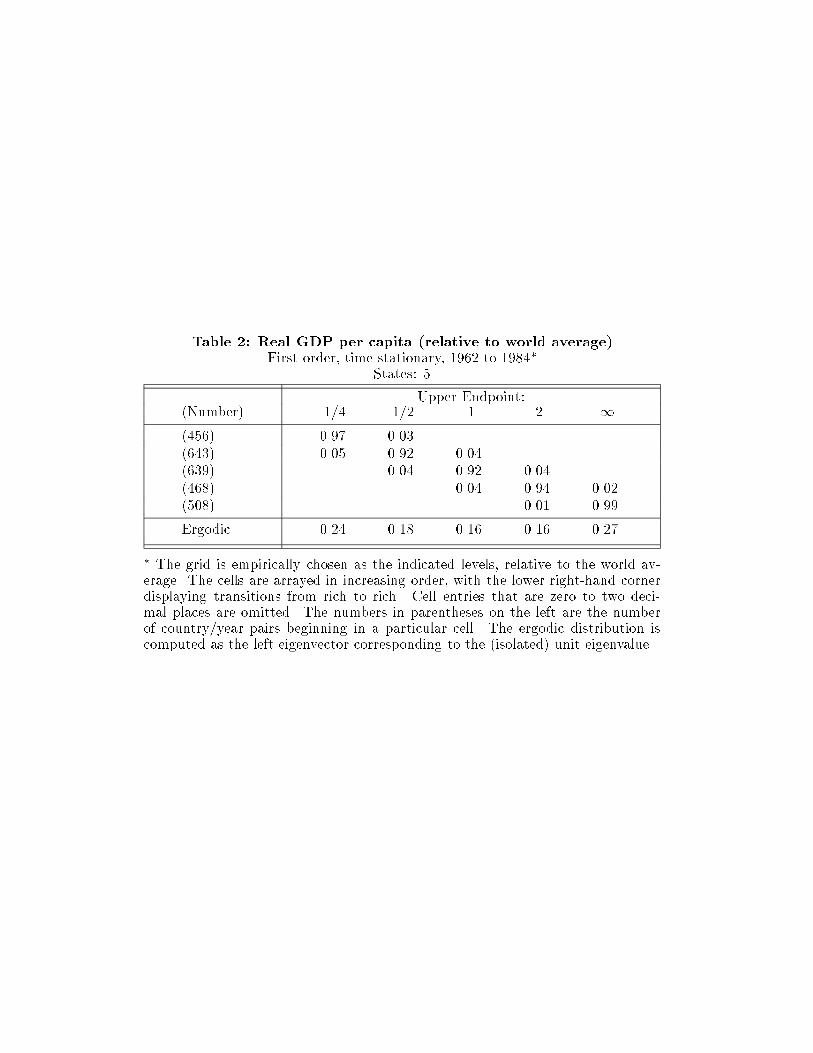
Table 2: Real GDP per capita (relative to world average)First order, time-stationary, 1962 to 1984�
States: 5
Upper Endpoint:(Number) 1=4 1=2 1 2 1
(456) 0.97 0.03
(643) 0.05 0.92 0.04
(639) 0.04 0.92 0.04
(468) 0.04 0.94 0.02
(508) 0.01 0.99
Ergodic 0.24 0.18 0.16 0.16 0.27
� The grid is empirically chosen as the indicated levels, relative to the world av-erage. The cells are arrayed in increasing order, with the lower right-hand cornerdisplaying transitions from rich to rich. Cell entries that are zero to two deci-mal places are omitted. The numbers in parentheses on the left are the numberof country/year pairs beginning in a particular cell. The ergodic distribution iscomputed as the left eigenvector corresponding to the (isolated) unit eigenvalue.
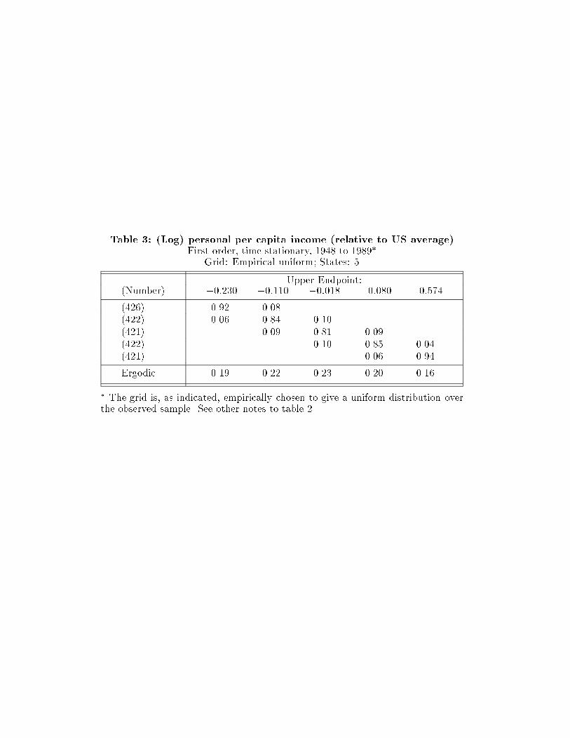
Table 3: (Log) personal per capita income (relative to US average)First order, time-stationary, 1948 to 1989�
Grid: Empirical uniform; States: 5
Upper Endpoint:(Number) �0:230 �0:110 �0:018 0:080 0:574
(426) 0.92 0.08
(422) 0.06 0.84 0.10
(421) 0.09 0.81 0.09
(422) 0.10 0.85 0.04
(421) 0.06 0.94
Ergodic 0.19 0.22 0.23 0.20 0.16
� The grid is, as indicated, empirically chosen to give a uniform distribution overthe observed sample. See other notes to table 2.

Y
t
Figure 3.1: �-divergence towards �-convergent steady state
Yj
Yk
Yj
Yk
Y
t
steady state
Figure 3.2: Coincident � and � convergence
large, perturbing disturbance
smooth monotone transition
Y
t
Figure 3.3: �-convergent limit with criss-crossing
Yj
Yk
Y
t
Figure 3.4: �-convergent limit with persistent inequality
Yj
Yk
�0 �t = �0
increasing income values
time
Figure 4.1: Evolving distributions, tending towards bimodal
income distributions
t0 t1
Recommended