Download pdf - Efficient Tools for the Simulation of Flapping Wing … · Efficient tools for the simulation of flapping ... for lift and propulsion using flapping wings ... of th e ß ow is the

E!cient tools for the simulation of flapping wing flows

Je! D. Eldredge!

Mechanical & Aerospace Engineering Department, University of California, Los Angeles,Los Angeles, CA 90095-1597

The development of novel strategies for lift and propulsion using flapping wings requiresthe use of computational tools that are at once e!cient and capable of handling complexdeforming boundary motion. In this work we present the use of a viscous vortex particlemethod for the simulation of the flow produced by a two-dimensional rigid wing in pitch-ing and plunging motion of moderate Reynolds number. By its Lagrangian nature, thismethod is able to automatically adapt to important flow structures. E!ciency is ensuredby using vorticity-bearing computational elements that are distributed only to the extentthat vorticity itself is spread through its convection and di"usion; no e"ort is needed forirrotational regions of flow. Moreover, the correct behavior of the velocity at infinity isautomatically satisfied, obviating the need for an artificial boundary treatment. Results ofthe dynamically shed vorticity and the forces exerted are presented for a single stroke of aflapping elliptical wing.

I. Motivation

Research in biologically-inspired mechanisms for propulsion has increased considerably in recent years, duein large part to a growing interest in developing micro air vehicles (MAVs) with capabilities that exceedthose of conventional aircraft: for example, carrying out remote sensing while flying in a confined space.Airborne insects are a natural paradigm for such vehicles, as they are equipped for an amazing range ofmaneuvers: hovering, flying backward, and rapidly changing trajectory.

Placing such demands on a technological equivalent requires a thorough knowledge of the fluid dynamicsinvolved. To develop an understanding of the physics of a flapping wing, as well as to provide a basis withwhich control strategies can be developed, a set of e!cient and accurate computational tools is essential. Inthis spirit, we present here the application of a vortex particle method for solving the viscous incompressibleflow around a two-dimensional flapping wing.

Computational investigations of a single flapping wing have been carried out by a number of researchers,for instance by Ramamurti & Sandberg,1,2 Liu & Kawachi3 and Wang.4 The flow produced by a flappingwing is highly unsteady and dominated by vortex shedding at its leading and trailing edges. Consequently,many investigators use a grid-based approach in vorticity-streamfunction formulation. However, conventionalgrid-based simulations are di!cult, due to the complication of (perhaps multiple) moving boundaries, whichrequires that the grid be continually regenerated in response to such motion. A notable exception is the recentwork of Russell & Wang,5 in which the surfaces of moving objects impose conditions that are interpolated

!Assistant Professor, Mechanical & Aerospace Engineering, University of California, Los Angeles, Los Angeles, CA, 90095-1597, email: [email protected]. Member, AIAA.

1 of 11

American Institute of Aeronautics and Astronautics

43rd AIAA Aerospace Sciences Meeting and Exhibit10 - 13 January 2005, Reno, Nevada

AIAA 2005-85

Copyright © 2005 by Jeff D. Eldredge. Published by the American Institute of Aeronautics and Astronautics, Inc., with permission.

to the control points of a regular Cartesian grid. Even with this capability, the use of a grid requires thata choice be made about its outer truncation, as well as the explicit introduction of an artificial boundarycondition to ensure the correct behavior at infinity.

The vortex particle method, in contrast, is based on a Lagrangian approach, wherein computational elements—or particles—are identified with material elements and thus move with the flow. These particles each carrya distribution of vorticity; the velocity field of the flow is the superposition of all particles’ contributionsthrough the Biot-Savart integral. Since particles, in a sense, define the flow rather than merely sample it,they are able to automatically adapt to the important features. They are only present in regions of non-zerovorticity, so no computational e!ort is wasted on irrotational regions. The computation of velocity throughthe Biot-Savart integral ensures that the boundary condition at infinity is automatically satisfied. Finally,the simulation of flows produced by complex moving, deformable boundaries presents no significant challengebeyond those encountered in the flow around a rigid, stationary object.

In this work, a viscous vortex particle method is applied to simulate the flow produced by two-dimensionalbodies in arbitrary motion. In section II, the methodology and practical aspects of the simulation tool arebriefly described. Results from applying the tool to a pitching, plunging elliptical wing are presented insection III. Finally, future directions are discussed in section IV.

II. Methodology

The use of the vortex particle method to compute viscous flows around objects was first presented byChorin,6 in whose method the vorticity produced by the body was carried away by newly-created particles,and di!usion was simulated by a random walk. The more recent work of Koumoutsakos, Leonard andPepin7 exhibited its utility as a tool for high fidelity simulation. Instead of creating new particles at the body,vorticity is introduced by di!usion onto existing particles. The techniques developed in their work have sincebeen refined, and the state of the art expounded in detail in the recent book by Cottet and Koumoutsakos.8The basic principles of the method are merely outlined here, with specialty to two dimensional flow.

A. Vortex particles

The vorticity field is regarded as the composition of a set of regularized vortex particles,

!(x, t) =!

p

"p(t)"!(x! xp(t)), (1)

where "p is the strength of the particle and xp is its position. The vorticity distribution of each particle isgiven by "!, which is generally radially symmetric, and # is the radius of the distribution. Particles are initiallylaid on a uniform Cartesian grid of spacing $x, and the particle strengths set to "p(0) = $x2!(xp(0), 0). Theparticles then move with the local value of the velocity field,

dxp

dt= u(xp, t). (2)

This velocity field is related to the vorticity through the inversion of ! = "# u, which is provided by theBiot-Savart integral, plus any additional potential flow (e.g. uniform flow)

u(x, t) =12%

"!(x!, t)

|x! x!|2

#!(y ! y!)x! x!

$dx! +"&. (3)

2 of 11


When the regularized vorticity (1) is introduced to this integral, the velocity field is expressed as a sum ofall particles’ contributions, so each particle evolves according to

dxp

dt=

!

q

"q(t)K!(xp(t)! xq(t)) +"&, (4)

where K! is a regularized, discrete Biot-Savart kernel. Thus, the regularizing function "! serves the dualpurpose of providing a smooth vorticity distribution for each particle, and eliminating the velocity singularitybetween two particles whose separation shrinks to zero. For stability, the method requires that particlesoverlap (i.e., # $ $x). It is important to note that, by computing the velocity via (4), its correct behavior atinfinity is automatically satisfied.

For an inviscid flow, equation (4) is closed due to the invariance of vorticity of material elements. However,in a viscous incompressible flow the vorticity of a material element is governed by

D!

Dt= '"2!. (5)

In the present method, the di!usive action is accounted for through modification of the particle strengths, viaan evolution equation that is the discrete analog of (5). In order to ensure that this di!usion is conservativeof the global circulation, the method of particle strength exchange9 is used, which replaces the Laplacianoperator of (5) with a symmetric integral operator. Upon particle quadrature of the integral, the resultingequation for the particle strengths is

d"p

dt=

'

#2

!

q

("q ! "p)(!(xp ! xq). (6)

The kernel (! can be constructed so that the integral operator approximates the Laplacian operator to anyorder of accuracy.10 In a given discrete time step, equation (6) is solved after the particle position equation(2) is evolved (i.e. a viscous splitting), resulting in a method for the direct numerical simulation of viscousincompressible flow.

B. Enforcing wall boundary conditions

The algorithm described thus far can be used to simulate unbounded viscous flows, but the inclusion ofbounding surfaces requires further treatment, in order to enforce the conditions of no-through-flow and no-slipat the surfaces. In a vorticity-based method, such a task is not straightforward, but crucial nonetheless—particularly because the no-slip condition is the primary mechanism for vorticity production in flows ofpresent interest.

Though there are several techniques for accounting for a no-slip surface in vortex methods, nearly all arebased on the Lighthill creation mechanism.11 He focused on the production of vorticity in a small interval oftime: At the beginning of the interval, the vorticity already present in the flow has a corresponding velocitythat has the correct wall normal component, but in general, slips relative to the wall. Therefore, the vorticitycreated during the subsequent interval must be exactly that needed to cancel this spurious slip velocity.

The algorithm used by Koumoutsakos et al.7 involves a fractional step procedure that embodies this creationmechanism. In the first half-step, vortex particles move and exchange strength according to the unboundedflow algorithm above. In the second half-step, a vortex sheet is created at the wall, with a strength distribu-tion that is determined by the no-through-flow condition (using a vortex panel method as in aerodynamics).By ‘displacing’ this vortex sheet from the wall into the flow, the no slip condition is also enforced under thesheet. This displacement is e!ected by the di!usion of the panel strengths onto existing particles adjacent

3 of 11


to the wall, through solution of the di!usion equation with the Neumann boundary condition

')!

)n= !*(s)

$t, (7)

where *(s) is the local sheet circulation, $t is the time step size and n is the normal vector directed into theflow.

It is vital that the solution for the surface panel strengths be carried out with consideration of Kelvin’stheorem, that the sum of flow and body circulation must remain zero for all time. A rigid rotating body hascirculation equal to !2Ab+(t), where Ab is the area of the two-dimensional body and !+(t) is its angularvelocity (the negative sign is included to identify + with the rate of change of conventional angle of incidence).Thus the constraint on the flow circulation is

d"tot

dt= 2Ab

d+

dt, (8)

where "tot =%

p "p, the sum of all particle strengths. The circulation of the flow is augmented at each timestep by the di!usion of the surface vortex sheet. By integrating (5) over the flow domain, the rate of changeof "tot is given by

d"tot

dt= !'

"

C

)!

)nds, (9)

where the right-hand integral is taken over the body surface. Combining these relations, the constraintimposed on the surface circulation introduced in time interval [t, t + $t] is

"

C*(s) ds = 2Ab (+(t + $t)! +(t)) . (10)

Rather than impose (10) in this form, however, we use a slightly di!erent form suggested by Ploumhans andWinckelmans:12 "

C*(s) ds = 2Ab+(t + $t)!

!

p

""p(t), (11)

where ""p(t) are the strengths of the particles at the end of the first (unbounded flow) half-step. This approach

compensates for circulation leaks in other components of the algorithm, for example due to the interpolationof particle strength into the body during the particle re-initialization phase described below.

C. Other aspects

The particle evolution and strength exchange, coupled with the surface vortex sheet di!usion, constitute acomplete algorithm for the solution of viscous, wall-bounded incompressible flows. In its practical imple-mentation, the fast multipole method13 is used to accelerate the evaluation of the velocity field in (4) toO(N), from its direct O(N2) form which is prohibitive of large simulations. A tree code is used to define ahierarchy of particle clusters that interact only through multipole expansions about their centers.

The flow map often contains local stagnation points that will cause some particles to cluster and othersto disperse. Such behavior tends to degrade the long-term accuracy (and stability) of a particle-basedsimulation. Severe particle distortion is prevented in the present method by re-initializing the particleconfiguration every few time steps. In this procedure, the strengths of the old particles are interpolatedonto new particle locations that are arranged on a Cartesian grid. We use the M !

4 interpolation kernel—developed by Monaghan14 for smoothed particle hydrodynamics—which ensures the conservation of the firstthree discrete moments of vorticity. The new configuration is then trimmed of particles whose strengths,as well as those of all its neighbors within a viscous radius C

%'$t, are smaller than some tolerance. This

4 of 11


UpstrokeDownstroke

Plun

ging

Pitc

hing

!d

!u

Angle of attack

A/2

-A/2

0

Win

g tr

ansv

erse

pos

ition

-1

1

0

0 1Cycle

Plun

ging

vel

ocity

Pitching angular velocity-!0.

!0.

0

Downstroke Upstroke Downstroke

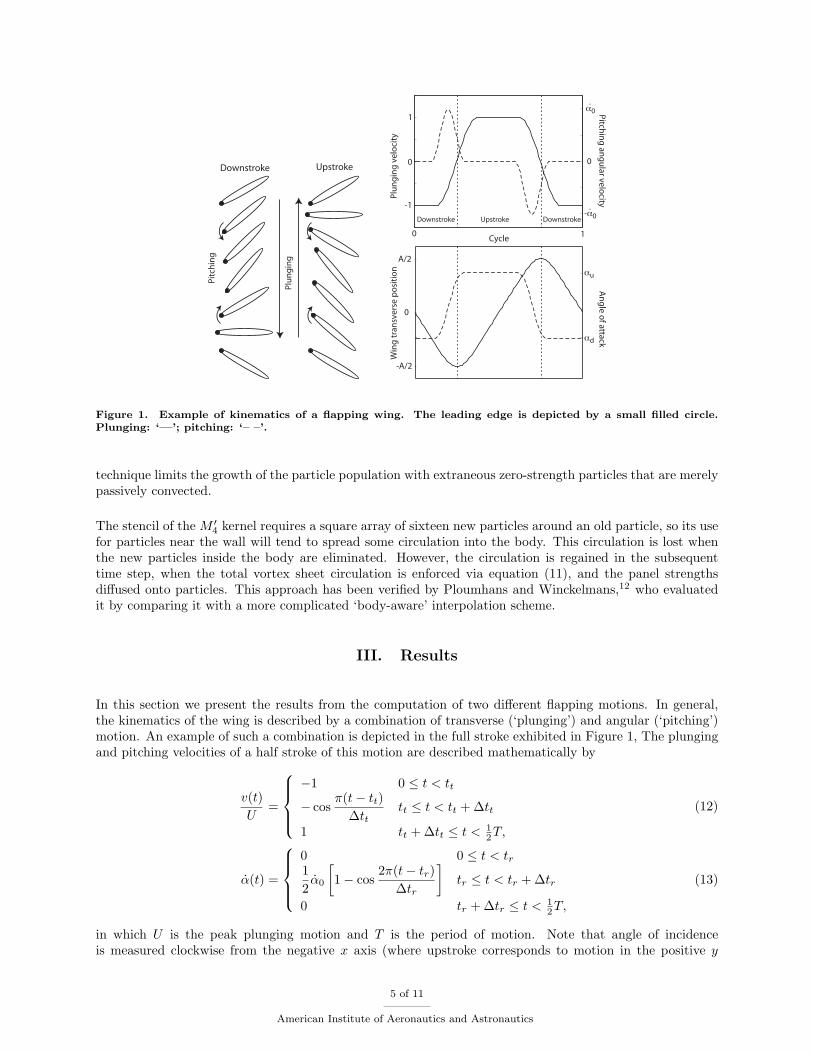
Figure 1. Example of kinematics of a flapping wing. The leading edge is depicted by a small filled circle.Plunging: ‘—’; pitching: ‘– –’.

technique limits the growth of the particle population with extraneous zero-strength particles that are merelypassively convected.

The stencil of the M !4 kernel requires a square array of sixteen new particles around an old particle, so its use

for particles near the wall will tend to spread some circulation into the body. This circulation is lost whenthe new particles inside the body are eliminated. However, the circulation is regained in the subsequenttime step, when the total vortex sheet circulation is enforced via equation (11), and the panel strengthsdi!used onto particles. This approach has been verified by Ploumhans and Winckelmans,12 who evaluatedit by comparing it with a more complicated ‘body-aware’ interpolation scheme.

III. Results

In this section we present the results from the computation of two di!erent flapping motions. In general,the kinematics of the wing is described by a combination of transverse (‘plunging’) and angular (‘pitching’)motion. An example of such a combination is depicted in the full stroke exhibited in Figure 1, The plungingand pitching velocities of a half stroke of this motion are described mathematically by

v(t)U

=

&''(

'')

!1 0 & t < tt

! cos%(t! tt)

#tttt & t < tt + #tt

1 tt + #tt & t < 12T,

(12)

+(t) =

&''(

'')

0 0 & t < tr12+0

*1! cos

2%(t! tr)#tr

+tr & t < tr + #tr

0 tr + #tr & t < 12T,

(13)

in which U is the peak plunging motion and T is the period of motion. Note that angle of incidenceis measured clockwise from the negative x axis (where upstroke corresponds to motion in the positive y

5 of 11


direction). Motion of this sort was imposed, for example, by Dickinson et al.15 on their mechanical wingapparatus. After an interval of constant plunging velocity during the downstroke, the wing decelerates andchanges direction. The wing then accelerates on the upstroke to the same constant velocity, decelerates, thenchanges direction again. The wing angle of incidence remains constant at +d for a portion of the downstroke,then the leading edge rotates clockwise (supinates) during the transition from downstroke and upstroke. Thewing maintains a new constant angle of incidence +u for a portion of the upstroke, then begins to rotatecounter-clockwise (pronates) just prior to the downstroke.

The free parameters that describe this motion are: the Strouhal number St = fc/U based on wing chord cand frequency f = 1/T ; the extreme angles of incidence +d and +u; the interval of direction change, #tt; theinterval of angle of incidence change, #tr; and #tlag, the time by which the instant of direction change lagsthe instant of peak pitching. The other times are then given by tt = 1

4T ! 12#tt and tr = 1

4T ! 12#tr!#tlag.

The peak pitching speed is given by +0 = 2(+u ! +d)/#tr.

A. Case 1

In the first case, an elliptical wing with aspect ratio 5 and initial angle of incidence + = !40# is prescribedwith a pitching and plunging motion with Strouhal number St = 0.25. The intervals are #tt/T = 0.667,#tr/T = 0.333, and #tlag/T = 0.08, and the extreme angles of incidence are +u = 40# and +d = !40#. TheReynolds number based on the peak plunging velocity and wing chord, Re = Uc/', is 550. The particlespacing is uniformly $x/c = 0.005 and the time step size used for the fourth-order Runge-Kutta method isU$t/c = 0.005. The elliptical wing is discretized with 284 panels, each with size determined by mapping acorresponding uniform panel from a circle of diameter c, which ensures that panels are most refined near thewing tips. The simulation begins with a distribution of around 1000 zero-strength particles within a viscouslength scale of the wing. The vortex sheet established by the impulsive start is immediately di!used to theparticles, and the time-stepping is subsequently begun.

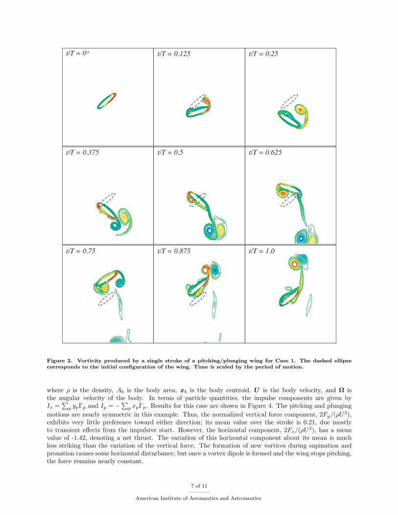
The simulation of one stroke required a computational time of ' 9.5hours and two strokes required '38hours on a single 2.2GHz Intel Xeon processor; this processing time can be decreased by using larger particlesas vortices travel far from the wing. At the end of the stroke the number of particles has grown to 2.6# 105.Note that no attempt was made to find the optimal particle spacing and time step size for this problem;the values used are likely too conservative. The economy of the method is most clearly demonstrated byFigure 3, which depicts the boundary of particle coverage at the end of the stroke. Particles are distributedonly as far as vorticity has spread by convection and di!usion. An equivalent simulation using a grid-basedscheme would require a much larger domain, with an external boundary for the enforcement of the conditionat infinity.

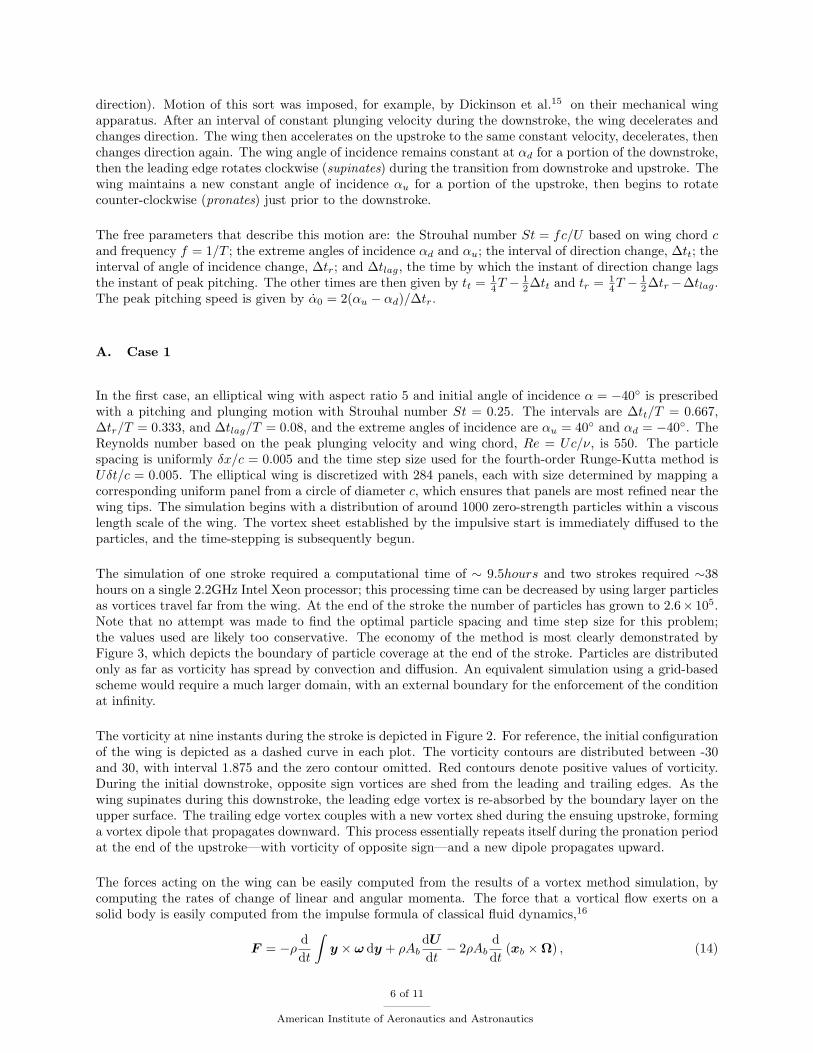
The vorticity at nine instants during the stroke is depicted in Figure 2. For reference, the initial configurationof the wing is depicted as a dashed curve in each plot. The vorticity contours are distributed between -30and 30, with interval 1.875 and the zero contour omitted. Red contours denote positive values of vorticity.During the initial downstroke, opposite sign vortices are shed from the leading and trailing edges. As thewing supinates during this downstroke, the leading edge vortex is re-absorbed by the boundary layer on theupper surface. The trailing edge vortex couples with a new vortex shed during the ensuing upstroke, forminga vortex dipole that propagates downward. This process essentially repeats itself during the pronation periodat the end of the upstroke—with vorticity of opposite sign—and a new dipole propagates upward.

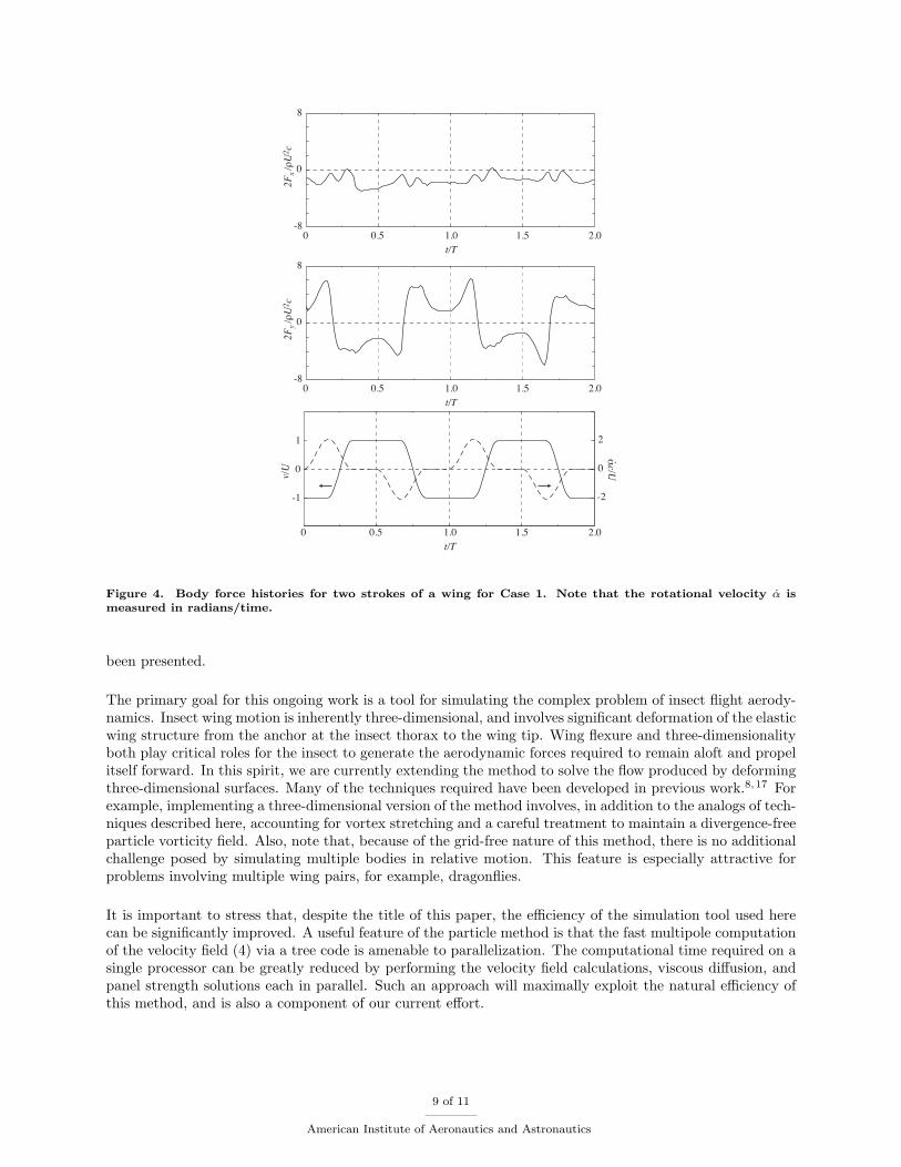
The forces acting on the wing can be easily computed from the results of a vortex method simulation, bycomputing the rates of change of linear and angular momenta. The force that a vortical flow exerts on asolid body is easily computed from the impulse formula of classical fluid dynamics,16

F = !,ddt

"y # ! dy + ,Ab

dU

dt! 2,Ab

ddt

(xb #!) , (14)

6 of 11


t/T = 0+ t/T = 0.125 t/T = 0.25

t/T = 0.375 t/T = 0.5 t/T = 0.625

t/T = 0.75 t/T = 0.875 t/T = 1.0

Figure 2. Vorticity produced by a single stroke of a pitching/plunging wing for Case 1. The dashed ellipsecorresponds to the initial configuration of the wing. Time is scaled by the period of motion.

where , is the density, Ab is the body area, xb is the body centroid, U is the body velocity, and ! isthe angular velocity of the body. In terms of particle quantities, the impulse components are given byIx =

%p yp"p and Iy = !

%p xp"p. Results for this case are shown in Figure 4. The pitching and plunging

motions are nearly symmetric in this example. Thus, the normalized vertical force component, 2Fy/(,U2),exhibits very little preference toward either direction; its mean value over the stroke is 0.21, due mostlyto transient e!ects from the impulsive start. However, the horizontal component, 2Fx/(,U2), has a meanvalue of -1.42, denoting a net thrust. The variation of this horizontal component about its mean is muchless striking than the variation of the vertical force. The formation of new vortices during supination andpronation causes some horizontal disturbance, but once a vortex dipole is formed and the wing stops pitching,the force remains nearly constant.

7 of 11


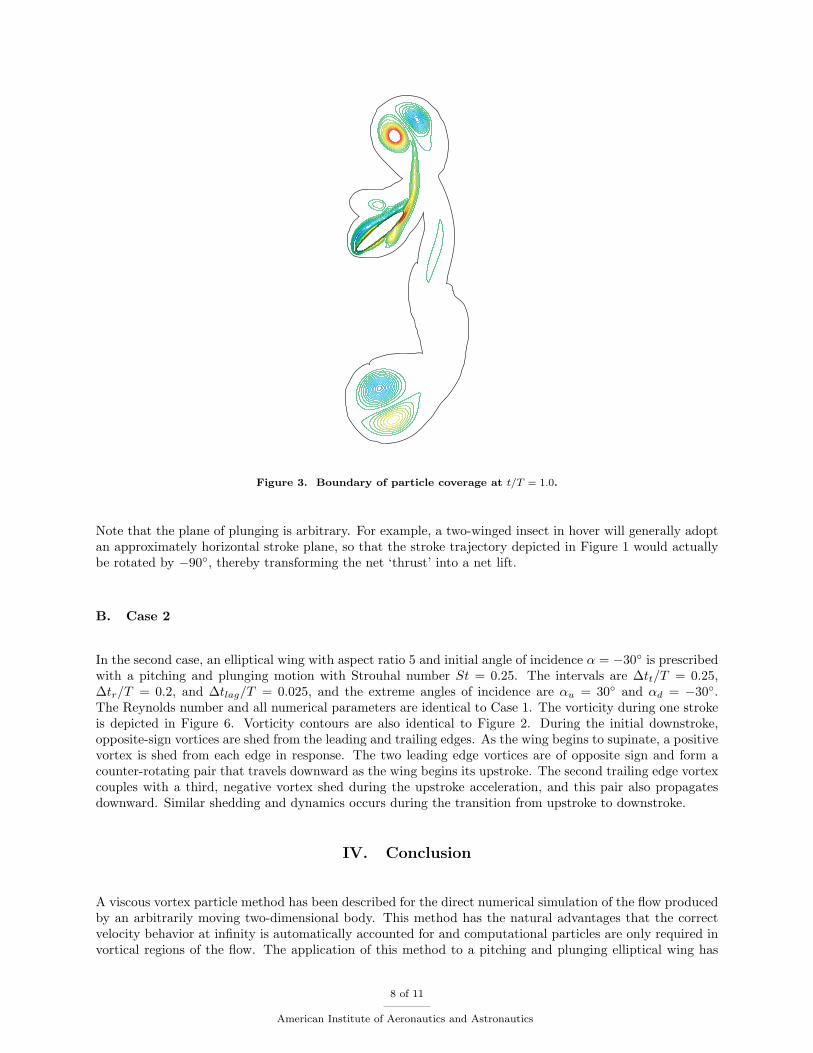
Figure 3. Boundary of particle coverage at t/T = 1.0.

Note that the plane of plunging is arbitrary. For example, a two-winged insect in hover will generally adoptan approximately horizontal stroke plane, so that the stroke trajectory depicted in Figure 1 would actuallybe rotated by !90#, thereby transforming the net ‘thrust’ into a net lift.

B. Case 2

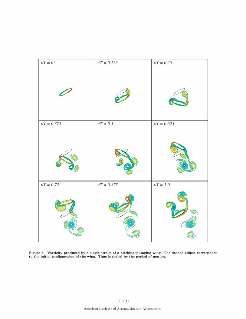
In the second case, an elliptical wing with aspect ratio 5 and initial angle of incidence + = !30# is prescribedwith a pitching and plunging motion with Strouhal number St = 0.25. The intervals are #tt/T = 0.25,#tr/T = 0.2, and #tlag/T = 0.025, and the extreme angles of incidence are +u = 30# and +d = !30#.The Reynolds number and all numerical parameters are identical to Case 1. The vorticity during one strokeis depicted in Figure 6. Vorticity contours are also identical to Figure 2. During the initial downstroke,opposite-sign vortices are shed from the leading and trailing edges. As the wing begins to supinate, a positivevortex is shed from each edge in response. The two leading edge vortices are of opposite sign and form acounter-rotating pair that travels downward as the wing begins its upstroke. The second trailing edge vortexcouples with a third, negative vortex shed during the upstroke acceleration, and this pair also propagatesdownward. Similar shedding and dynamics occurs during the transition from upstroke to downstroke.

IV. Conclusion

A viscous vortex particle method has been described for the direct numerical simulation of the flow producedby an arbitrarily moving two-dimensional body. This method has the natural advantages that the correctvelocity behavior at infinity is automatically accounted for and computational particles are only required invortical regions of the flow. The application of this method to a pitching and plunging elliptical wing has

8 of 11


0 0.5 1.0 1.5 2.0-8

8

0

2Fx

/!U

2 c

t/T

0 0.5 1.0 1.5 2.0-8

8

0

2Fy

/!U

2 c

t/T

0 0.5 1.0 1.5 2.0t/T

1

0

-1 -2

2

0

!c/U.

v/U

Figure 4. Body force histories for two strokes of a wing for Case 1. Note that the rotational velocity ! ismeasured in radians/time.

been presented.

The primary goal for this ongoing work is a tool for simulating the complex problem of insect flight aerody-namics. Insect wing motion is inherently three-dimensional, and involves significant deformation of the elasticwing structure from the anchor at the insect thorax to the wing tip. Wing flexure and three-dimensionalityboth play critical roles for the insect to generate the aerodynamic forces required to remain aloft and propelitself forward. In this spirit, we are currently extending the method to solve the flow produced by deformingthree-dimensional surfaces. Many of the techniques required have been developed in previous work.8,17 Forexample, implementing a three-dimensional version of the method involves, in addition to the analogs of tech-niques described here, accounting for vortex stretching and a careful treatment to maintain a divergence-freeparticle vorticity field. Also, note that, because of the grid-free nature of this method, there is no additionalchallenge posed by simulating multiple bodies in relative motion. This feature is especially attractive forproblems involving multiple wing pairs, for example, dragonflies.

It is important to stress that, despite the title of this paper, the e$ciency of the simulation tool used herecan be significantly improved. A useful feature of the particle method is that the fast multipole computationof the velocity field (4) via a tree code is amenable to parallelization. The computational time required on asingle processor can be greatly reduced by performing the velocity field calculations, viscous di!usion, andpanel strength solutions each in parallel. Such an approach will maximally exploit the natural e$ciency ofthis method, and is also a component of our current e!ort.

9 of 11


5

0

-50 0.5 1.0 1.5 2.0

t/T

2Fx

/!U

2 c8

0

-80 0.5 1.0 1.5 2.0

t/T

2Fy

/!U

2 c

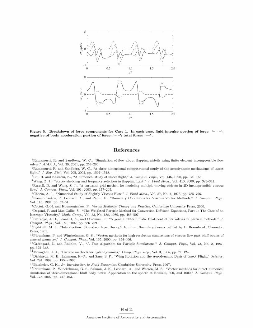
Figure 5. Breakdown of force components for Case 1. In each case, fluid impulse portion of force: ‘– · –’;negative of body acceleration portion of force: ‘– –’; total force: ‘—’ .

References

1Ramamurti, R. and Sandberg, W. C., “Simulation of flow about flapping airfoils using finite element incompressible flowsolver,” AIAA J., Vol. 39, 2001, pp. 253–260.2Ramamurti, R. and Sandberg, W. C., “A three-dimensional computational study of the aerodynamic mechanisms of insect

flight,” J. Exp. Biol., Vol. 205, 2002, pp. 1507–1518.3Liu, H. and Kawachi, K., “A numerical study of insect flight,” J. Comput. Phys., Vol. 146, 1998, pp. 125–156.4Wang, Z. J., “Vortex shedding and frequency selection in flapping flight,” J. Fluid Mech., Vol. 410, 2000, pp. 323–341.5Russell, D. and Wang, Z. J., “A cartesian grid method for modeling multiple moving objects in 2D incompressible viscous

flow,” J. Comput. Phys., Vol. 191, 2003, pp. 177–205.6Chorin, A. J., “Numerical Study of Slightly Viscous Flow,” J. Fluid Mech., Vol. 57, No. 4, 1973, pp. 785–796.7Koumoutsakos, P., Leonard, A., and Pepin, F., “Boundary Conditions for Viscous Vortex Methods,” J. Comput. Phys.,

Vol. 113, 1994, pp. 52–61.8Cottet, G.-H. and Koumoutsakos, P., Vortex Methods: Theory and Practice, Cambridge University Press, 2000.9Degond, P. and Mas-Gallic, S., “The Weighted Particle Method for Convection-Di!usion Equations, Part 1: The Case of an

Isotropic Viscosity,” Math. Comp., Vol. 53, No. 188, 1989, pp. 485–507.10Eldredge, J. D., Leonard, A., and Colonius, T., “A general deterministic treatment of derivatives in particle methods,” J.Comput. Phys., Vol. 180, 2002, pp. 686–709.11Lighthill, M. J., “Introduction: Boundary layer theory,” Laminar Boundary Layers, edited by L. Rosenhead, ClarendonPress, 1961.12Ploumhans, P. and Winckelmans, G. S., “Vortex methods for high-resolution simulations of viscous flow past blu! bodies ofgeneral geometry,” J. Comput. Phys., Vol. 165, 2000, pp. 354–406.13Greengard, L. and Rokhlin, V., “A Fast Algorithm for Particle Simulations,” J. Comput. Phys., Vol. 73, No. 2, 1987,pp. 325–348.14Monaghan, J. J., “Particle methods for hydrodynamics,” Comp. Phys. Rep., Vol. 3, 1985, pp. 71–124.15Dickinson, M. H., Lehmann, F.-O., and Sane, S. P., “Wing Rotation and the Aerodynamic Basis of Insect Flight,” Science,Vol. 284, 1999, pp. 1954–1960.16Batchelor, G. K., An Introduction to Fluid Dynamics, Cambridge University Press, 1967.17Ploumhans, P., Winckelmans, G. S., Salmon, J. K., Leonard, A., and Warren, M. S., “Vortex methods for direct numericalsimulation of three-dimensional blu! body flows: Application to the sphere at Re=300, 500, and 1000,” J. Comput. Phys.,Vol. 178, 2002, pp. 427–463.

10 of 11


t/T = 0+ t/T = 0.125 t/T = 0.25

t/T = 0.375 t/T = 0.5 t/T = 0.625

t/T = 0.75 t/T = 0.875 t/T = 1.0

Figure 6. Vorticity produced by a single stroke of a pitching/plunging wing. The dashed ellipse correspondsto the initial configuration of the wing. Time is scaled by the period of motion.

11 of 11
