Download pdf - Edexcel GCSE Geography Controlled Assessment …api.ning.com/files/IlN0UevPKmZmrLiachYUtffJ3HIIW7...Edexcel GCSE Geography Controlled Assessment Exemplar 2014 Planning and methodology

Edexcel GCSE Geography Controlled Assessment Exemplar 2014

Example Task Question: The channel characteristics of a river change along its course.

Purpose Focus on velocity Sub- focus questions:

1. To what extent is there a regular /even change in velocity downstream? 2. Do changes in velocity downstream match the expectations of the

Bradshaw model? 3. What are the reasons for the change in velocity with progression

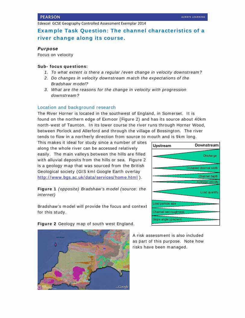
downstream? Location and background research The River Horner is located in the southwest of England, in Somerset. It is found on the northern edge of Exmoor (Figure 2) and has its source about 40km north-west of Taunton. In its lower course the river runs through Horner Wood, between Porlock and Allerford and through the village of Bossington. The river tends to flow in a northerly direction from source to mouth and is 9km long. This makes it ideal for study since a number of sites along the whole river can be accessed relatively easily. The main valleys between the hills are filled with alluvial deposits from the hills or sea. Figure 2 is a geology map that was sourced from the British Geological society (GIS kml Google Earth overlay http://www.bgs.ac.uk/data/services/home.html ). Figure 1 (opposite) Bradshaw’s model (source: the internet) Bradshaw’s model will provide the focus and context for this study. Figure 2 Geology map of south west England.

A risk assessment is also included as part of this purpose. Note how risks have been managed.


Figure 3a Figure 3b Figure 3a Inset regional map. Figure3b location of the River Horner (source: OS and http://wtp2.appspot.com/wheresthepath.htm Scale – 1km = 1 square), Note, river is indicated in blue on the Figure 3b. Risk Assessment Hazard Risk Likelihood Control Traffic Hit by moving

vehicle Low Careful of

vehicles, cross at designated points; awareness

Rocky footpath and Uneven ground

Slipping and trips, scratches and cuts, twisting ankle

High Awareness and care, move slowly and watch out for each other

Ticks Limes disease and/or a bite

Medium Long sleeves and awareness

What are river characteristics? We

concluded that they could include: width,

depth, velocity, gradient, sediment size etc.

Velocity works as an important control factor

in all of this.


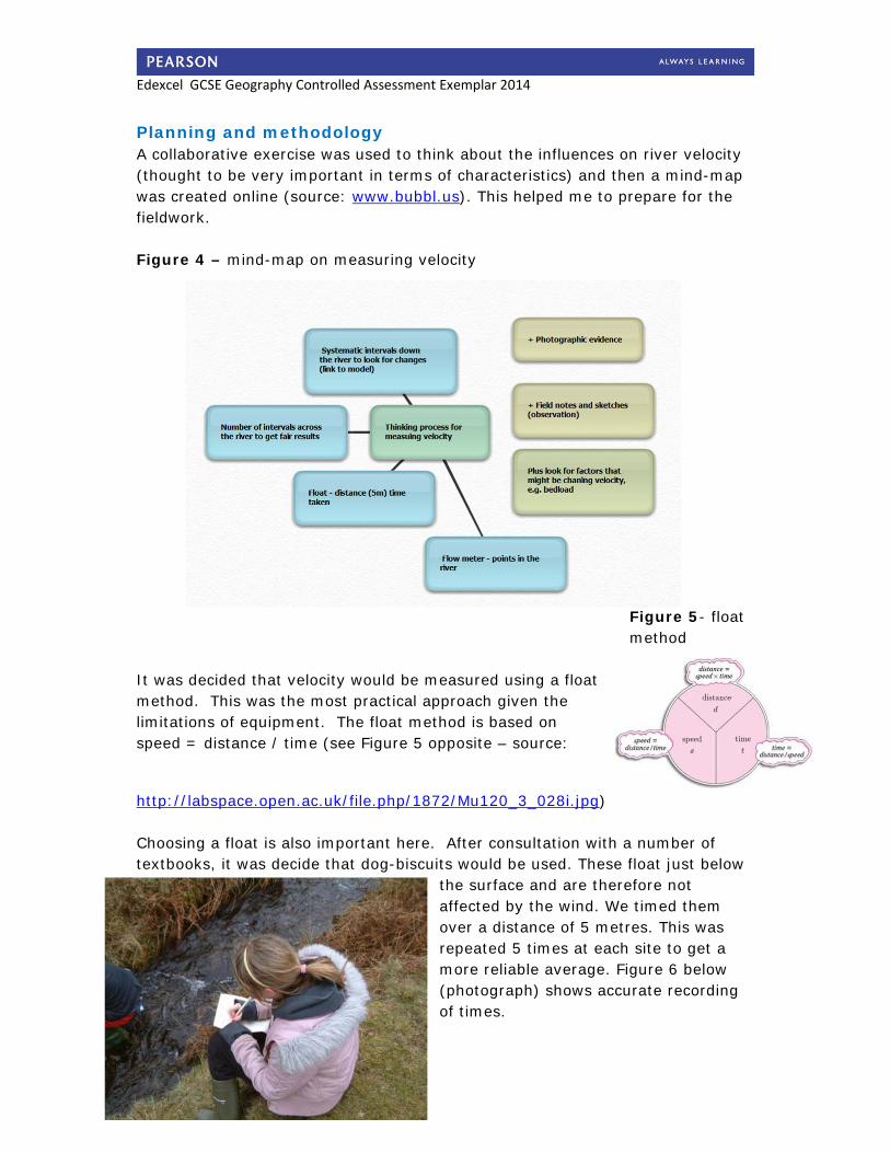
Planning and methodology A collaborative exercise was used to think about the influences on river velocity (thought to be very important in terms of characteristics) and then a mind-map was created online (source: www.bubbl.us). This helped me to prepare for the fieldwork. Figure 4 – mind-map on measuring velocity

Figure 5- float method

It was decided that velocity would be measured using a float method. This was the most practical approach given the limitations of equipment. The float method is based on speed = distance / time (see Figure 5 opposite – source:

http://labspace.open.ac.uk/file.php/1872/Mu120_3_028i.jpg) Choosing a float is also important here. After consultation with a number of textbooks, it was decide that dog-biscuits would be used. These float just below

the surface and are therefore not affected by the wind. We timed them over a distance of 5 metres. This was repeated 5 times at each site to get a more reliable average. Figure 6 below (photograph) shows accurate recording of times.


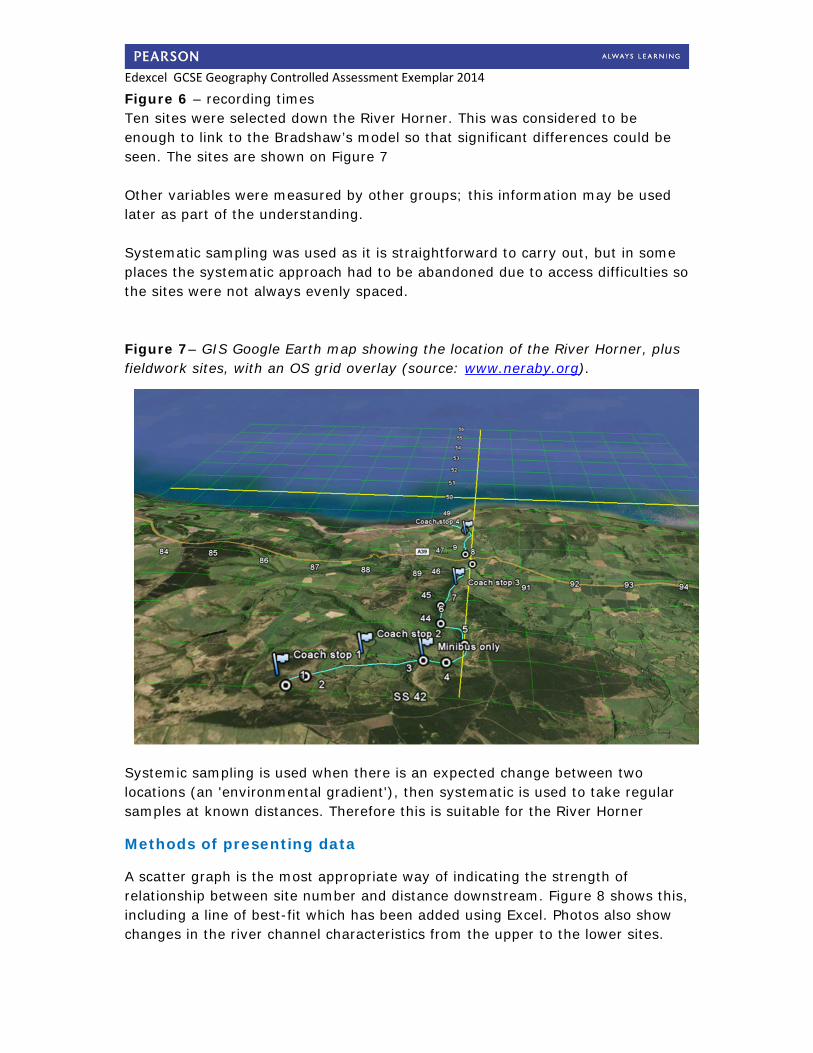
Figure 6 – recording times Ten sites were selected down the River Horner. This was considered to be enough to link to the Bradshaw’s model so that significant differences could be seen. The sites are shown on Figure 7 Other variables were measured by other groups; this information may be used later as part of the understanding. Systematic sampling was used as it is straightforward to carry out, but in some places the systematic approach had to be abandoned due to access difficulties so the sites were not always evenly spaced. Figure 7– GIS Google Earth map showing the location of the River Horner, plus fieldwork sites, with an OS grid overlay (source: www.neraby.org).

Systemic sampling is used when there is an expected change between two locations (an 'environmental gradient'), then systematic is used to take regular samples at known distances. Therefore this is suitable for the River Horner

Methods of presenting data

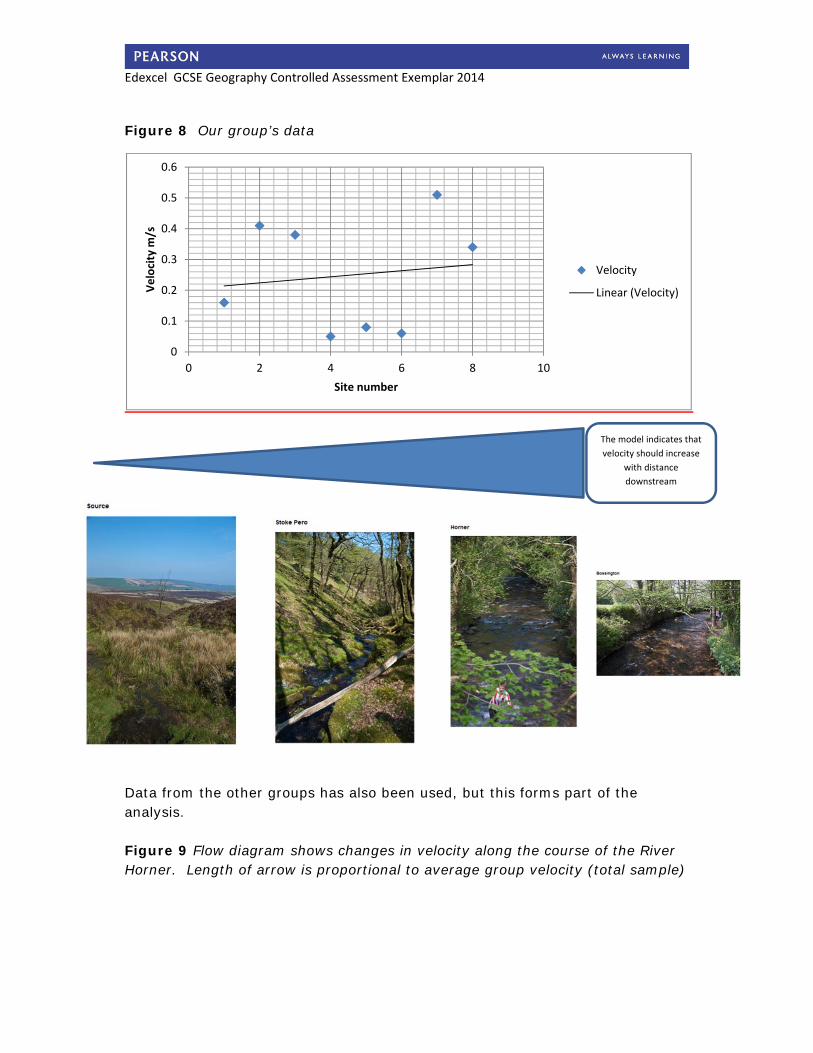
A scatter graph is the most appropriate way of indicating the strength of relationship between site number and distance downstream. Figure 8 shows this, including a line of best-fit which has been added using Excel. Photos also show changes in the river channel characteristics from the upper to the lower sites.


Figure 8 Our group’s data

Data from the other groups has also been used, but this forms part of the analysis. Figure 9 Flow diagram shows changes in velocity along the course of the River Horner. Length of arrow is proportional to average group velocity (total sample)

0

0.1

0.2

0.3

0.4

0.5

0.6

0 2 4 6 8 10

Velocity m

/s

Site number

Velocity

Linear (Velocity)

The model indicates that

velocity should increase

with distance

downstream


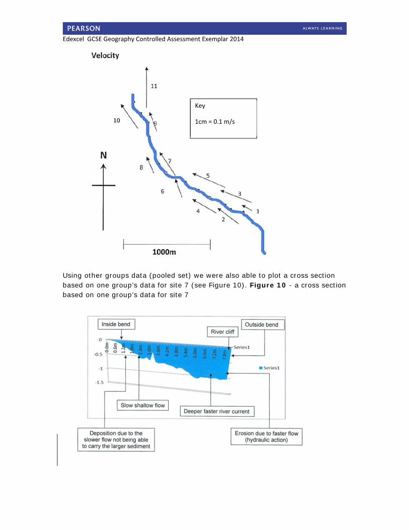
Using other groups data (pooled set) we were also able to plot a cross section based on one group’s data for site 7 (see Figure 10). Figure 10 - a cross section based on one group’s data for site 7

Key

1cm = 0.1 m/s


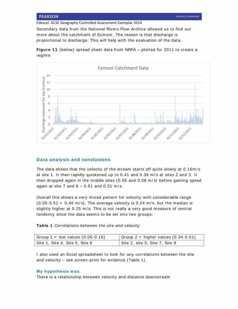
Secondary data from the National Rivers Flow Archive allowed us to find out more about the catchment of Exmoor. The reason is that discharge is proportional to discharge. This will help with the evaluation of the data.

Figure 11 (below) spread sheet data from NRFA – plotted for 2011 to create a regime

Data analysis and conclusions

The data shows that the velocity of the stream starts off quite slowly at 0.16m/s at site 1. It then rapidly quickened up to 0.41 and 0.38 m/s at sites 2 and 3. It then dropped again in the middle sites (0.05 and 0.08 m/s) before gaining speed again at site 7 and 8 – 0.51 and 0.31 m/s. Overall this shows a very mixed pattern for velocity with considerable range (0.05-0.51 = 0.46 m/s). The average velocity is 0.24 m/s, but the median is slightly higher at 0.25 m/s. This is not really a very good measure of central tendency since the data seems to be set into two groups: Table 1 Correlations between the site and velocity Group 1 = low values (0.05-0.16) Group 2 = higher values (0.34-0.51) Site 1, Site 4, Site 5, Site 6 Site 2, site 3, Site 7, Site 8 I also used an Excel spreadsheet to look for any correlations between the site and velocity – see screen-print for evidence (Table 1). My hypothesis was: There is a relationship between velocity and distance downstream

0

2

4

6

8

10

12

14

Discharge maxim

um for day (cumecs)

Exmoor Catchment Data


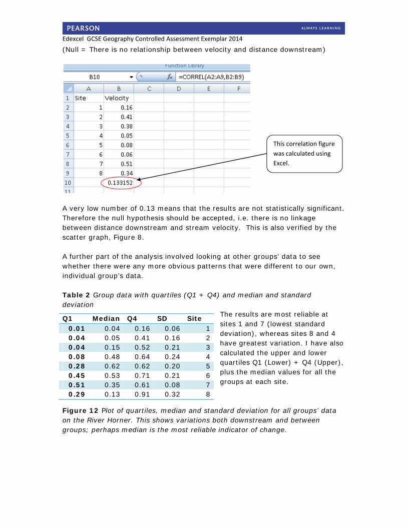
(Null = There is no relationship between velocity and distance downstream)

A very low number of 0.13 means that the results are not statistically significant. Therefore the null hypothesis should be accepted, i.e. there is no linkage between distance downstream and stream velocity. This is also verified by the scatter graph, Figure 8. A further part of the analysis involved looking at other groups’ data to see whether there were any more obvious patterns that were different to our own, individual group’s data. Table 2 Group data with quartiles (Q1 + Q4) and median and standard deviation

The results are most reliable at sites 1 and 7 (lowest standard deviation), whereas sites 8 and 4 have greatest variation. I have also calculated the upper and lower quartiles Q1 (Lower) + Q4 (Upper), plus the median values for all the groups at each site.

Figure 12 Plot of quartiles, median and standard deviation for all groups’ data on the River Horner. This shows variations both downstream and between groups; perhaps median is the most reliable indicator of change.

Q1 Median Q4 SD Site 0.01 0.04 0.16 0.06 1 0.04 0.05 0.41 0.16 2 0.04 0.15 0.52 0.21 3 0.08 0.48 0.64 0.24 4 0.28 0.62 0.62 0.20 5 0.45 0.53 0.71 0.21 6 0.51 0.35 0.61 0.08 7 0.29 0.13 0.91 0.32 8

This correlation figure

was calculated using

Excel.


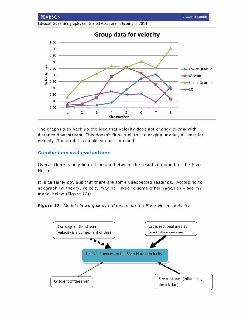
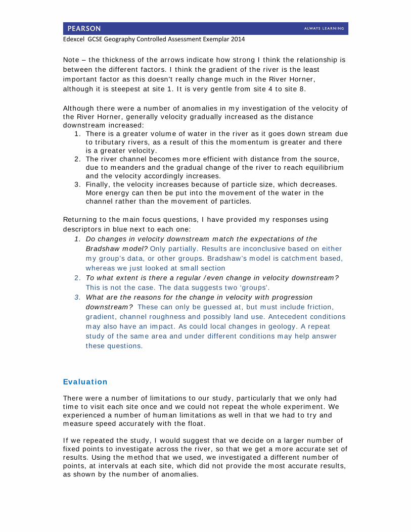
The graphs also back up the idea that velocity does not change evenly with distance downstream. This doesn’t fit so well to the original model, at least for velocity. The model is idealised and simplified. Conclusions and evaluations Overall there is only limited linkage between the results obtained on the River Horner. It is certainly obvious that there are some unexpected readings. According to geographical theory, velocity may be linked to some other variables – see my model below (Figure 13): Figure 13: Model showing likely influences on the River Horner velocity

0.00

0.10

0.20

0.30

0.40

0.50

0.60

0.70

0.80

0.90

1.00

1 2 3 4 5 6 7 8

Velocity m

/s

Site number

Group data for velocity

Lower Quartlie

Median

Upper Quartile

SD

Likely influences on the River Horner velocity

Discharge of the stream

(velocity is a component of this)

Cross sectional area at

point of measurement

Gradient of the river Size of stones (influencing

the friction)


Note – the thickness of the arrows indicate how strong I think the relationship is between the different factors. I think the gradient of the river is the least important factor as this doesn’t really change much in the River Horner, although it is steepest at site 1. It is very gentle from site 4 to site 8. Although there were a number of anomalies in my investigation of the velocity of the River Horner, generally velocity gradually increased as the distance downstream increased:

1. There is a greater volume of water in the river as it goes down stream due to tributary rivers, as a result of this the momentum is greater and there is a greater velocity.

2. The river channel becomes more efficient with distance from the source, due to meanders and the gradual change of the river to reach equilibrium and the velocity accordingly increases.

3. Finally, the velocity increases because of particle size, which decreases. More energy can then be put into the movement of the water in the channel rather than the movement of particles.

Returning to the main focus questions, I have provided my responses using descriptors in blue next to each one:

1. Do changes in velocity downstream match the expectations of the Bradshaw model? Only partially. Results are inconclusive based on either my group’s data, or other groups. Bradshaw’s model is catchment based, whereas we just looked at small section

2. To what extent is there a regular /even change in velocity downstream? This is not the case. The data suggests two ‘groups’.

3. What are the reasons for the change in velocity with progression downstream? These can only be guessed at, but must include friction, gradient, channel roughness and possibly land use. Antecedent conditions may also have an impact. As could local changes in geology. A repeat study of the same area and under different conditions may help answer these questions.

Evaluation

There were a number of limitations to our study, particularly that we only had time to visit each site once and we could not repeat the whole experiment. We experienced a number of human limitations as well in that we had to try and measure speed accurately with the float. If we repeated the study, I would suggest that we decide on a larger number of fixed points to investigate across the river, so that we get a more accurate set of results. Using the method that we used, we investigated a different number of points, at intervals at each site, which did not provide the most accurate results, as shown by the number of anomalies.


Data presentation was limited in some respects, e.g. only showing one cross section; assuming in Figures 8 and 11 that the sites were equidistant from each other (they were not). Secondary data was for the whole catchment rather than just this area, so once again it may not be fair to compare our results to a larger-scale drainage-basin. There are other pieces of data that could have been collected that would have taken the investigation further.

1. Larger number of sites; more measurements at each site would improve reliability.

2. More in depth analysis of channel roughness (hydraulic radius) as this is likely to affect velocity. This could have been measured at the same sites also.

3. If gradient is control over velocity then this should be measured. I could get this from a GIS map, as well as other group’s data.

4. Greater use of secondary data, e.g. other past projects, or monitoring stations.

5. More photographs would have provided greater evidence. To really improve the work, information could have been recorded from different times of year under different river flow (regime) conditions. Changes in velocity downstream may only be apparent, under higher flow conditions, for instance. This is when most sediment is moved and erosion takes place. Our results are a “snapshot” survey so we should question their validity, especially in the context of Figure 11. Overall channel characteristics do change along its course, but the relationship is far from simply predictable or easy to understand.