000

001

002

003

004

005

006

007

008

009

010

011

012

013

014

015

016

017

018

019

020

021

022

023

024

025

026

027

028

029

030

031

032

033

034

035

036

037

038

039

040

041

042

043

044

000

001

002

003

004

005

006

007

008

009

010

011

012

013

014

015

016

017

018

019

020

021

022

023

024

025

026

027

028

029

030

031

032

033

034

035

036

037

038

039

040

041

042

043

044

ECCV#ECCV 2012

Accepted PaperDraft

ECCV#ECCV 2012

Accepted PaperDraft

Camera Pose Estimation Using First-Order CurveDifferential Geometry

Ricardo Fabbri, Benjamin B. KimiaBrown University

Division of EngineeringProvidence RI 02912, USA

{rfabbri,kimia}@lems.brown.eduand

Peter J. GiblinUniversity of Liverpool

Liverpool, UKpjgiblin@liverpool.ac.uk

ECCV 2012 Accepted Paper Draft

Abstract. This paper considers and solves the problem of estimating camerapose given a pair of point-tangent correspondences between the 3D scene andthe projected image. The problem arises when considering curve geometry asthe basis of forming correspondences, computation of structure and calibration,which in its simplest form is a point augmented with the curve tangent. We showthat while the standard resectioning problem is solved with a minimum of threepoints given the intrinsic parameters, when points are augmented with tangentinformation only two points are required, leading to substantial computationalsavings, e.g., when used as a minimal engine within a RANSAC strategy. In ad-dition, computational algorithms are developed to find a practical and efficientsolution which is shown to effectively recover camera pose using synthetic andrealistic datasets. The resolution of this problem is intended as a basic buildingblock of future curve-based structure from motion systems, allowing new viewsto be incrementally registered to a core set of views for which relative pose hasalready been computed.

1 Introduction

A key problem in the reconstruction of structure from multiple views is the determina-tion of relative pose among cameras as well as the intrinsic parameters for each camera.The classical method is to rely on a set of corresponding points across views to deter-mine each camera’s intrinsic parameter matrix Kim as well as the relative pose betweenpairs of cameras [11]. The set of corresponding points can be determined using a cali-bration jig, but, more generally, using isolated keypoints such as Harris corners [10] orSIFT/HOG [17] features which remain somewhat stable over view and other variations.As long as there is a sufficient number of keypoints between two views, a random se-lection of a few feature correspondences using RANSAC [7,11] can be verified by mea-suring the number of inlier features. This class of isolated feature point-based methodsare currently in popular and successful use through packages such as the Bundler andused in applications such as Phototourism [1].

045

046

047

048

049

050

051

052

053

054

055

056

057

058

059

060

061

062

063

064

065

066

067

068

069

070

071

072

073

074

075

076

077

078

079

080

081

082

083

084

085

086

087

088

089

045

046

047

048

049

050

051

052

053

054

055

056

057

058

059

060

061

062

063

064

065

066

067

068

069

070

071

072

073

074

075

076

077

078

079

080

081

082

083

084

085

086

087

088

089

ECCV#ECCV 2012

Accepted PaperDraft

ECCV#ECCV 2012

Accepted PaperDraft

2 ECCV-12 Draft

(a) (c)

(b) (d)

Fig. 1. (a) Views with wide baseline separation may not have a sufficient number of interestpoints in common, but they often do share common curve structure. (b) There may not always besufficient interest points matching across views of homogeneous objects, such as for the sculpture,but there is sufficient curve structure. (c) Each moving object requires its own set of features, butthey may not be sufficient without a richly textured surface. (d) Non-rigid structures face the sameissue.

Two major drawbacks limit the applicability of automatic methods based on interestpoints. First, it is well-known that in practice the correlation of interest points works forviews with a limited baseline, according to some estimates no greater than 30◦ [18],Figure 1(a). In contrast, certain image curve fragments, e.g., those corresponding tosharp ridges, reflectance curves, etc, persist stably over a much larger range of views.Second, the success of interest point-based methods is based on the presence of anabundance of features so that a sufficient number of them survive the various variationsbetween views. While this is true in many scenes, as evidenced by the popularity of thisapproach, in a non-trivial number of scenes this is not the case, such as (i) Homogeneousregions, e.g., from man-made objects, corridors, etc., Figure 1(b); (ii) Multiple movingobjects require their own set of features which may not be sufficiently abundant withoutsufficient texture, Figure 1(c); (iii) Non-rigid objects require a rich set of features perroughly non-deforming patch, Figure 1(d). In all these cases, however, there is often

090

091

092

093

094

095

096

097

098

099

100

101

102

103

104

105

106

107

108

109

110

111

112

113

114

115

116

117

118

119

120

121

122

123

124

125

126

127

128

129

130

131

132

133

134

090

091

092

093

094

095

096

097

098

099

100

101

102

103

104

105

106

107

108

109

110

111

112

113

114

115

116

117

118

119

120

121

122

123

124

125

126

127

128

129

130

131

132

133

134

ECCV#ECCV 2012

Accepted PaperDraft

ECCV#ECCV 2012

Accepted PaperDraft

ECCV-12 Draft 3

(a)

Fig. 2. Challenges in using curve fragments in multiview geometry: (a) instabilitieswith slight changes in viewpoint, as shown for two views in (b) and zoomed in selec-tively in (c-h) showing real examples of edge grouping instabilities, such as a curve inone being broken into two in another view, a curve being linked onto background, acurve being detected in one view but absent in another, a curve being fragmented intovarious pieces at junctions in one view but fully linked in another view, different partsof a curve being occluded in different views, and a curve undergoing shape deformationfrom one view to the other. (i) Point correspondence ambiguity along the curve.

sufficient image curve structure, motivating augmenting the use of interest points bydeveloping a parallel technology for the use of image curve structure.

The use of image curves in determining camera pose has generally been based onepipolar tangencies, but these techniques assume that curves are closed or can be de-scribed as conics or other algebraic curves [14, 15, 19, 21]. The use of image curvefragments as the basic structure for auto-calibration under general conditions is facedwith two significant challenges. First, current edge linking procedures do not generallyproduce curve segments which persist stably across images. Rather, an image curvefragment in one view may be present in broken form and/or or grouped with other curvefragments. Thus, while the underlying curve geometry correlates well across views, theindividual curve fragments do not, Figure 2(a-h). Second, even when the image curvefragments correspond exactly, there is an intra-curve correspondence ambiguity, Fig-ure 2(i). This ambiguity prevents the use of corresponding curve points to solve for theunknown pose and intrinsic parameters. Both these challenges motivate the use of smallcurve fragments.

135

136

137

138

139

140

141

142

143

144

145

146

147

148

149

150

151

152

153

154

155

156

157

158

159

160

161

162

163

164

165

166

167

168

169

170

171

172

173

174

175

176

177

178

179

135

136

137

138

139

140

141

142

143

144

145

146

147

148

149

150

151

152

153

154

155

156

157

158

159

160

161

162

163

164

165

166

167

168

169

170

171

172

173

174

175

176

177

178

179

ECCV#ECCV 2012

Accepted PaperDraft

ECCV#ECCV 2012

Accepted PaperDraft

4 ECCV-12 Draft

Fig. 3. The problem of finding the camera pose R, T given space curves in a worldcoordinate system and their projections in an image coordinate system (left), and anapproach to that consisting of (right) finding the camera pose R, T given 3D point-tangents (i.e., local curve models) in a world coordinate system and their projections inan image coordinate system.

The paradigm explored in this paper is that small curve fragments, or equivalentlypoints augmented with differential-geometric attributes1, can be used as the basic imagestructure to correlate across views. The intent is to use curve geometry as a complemen-tary approach to the use of interest points in cases where these fail or are not available.The value of curve geometry is in correlating structure across three frames or more sincethe correspondence geometry in two views is unconstrained. However, the differentialgeometry at two corresponding points in two views reconstruct the differential geome-try of the space curve they arise from [4] and this constrains the differential geometryof corresponding curves in a third view.

The fundamental questions underlying the use of points augmented with differential-geometric attributes are: how many such points are needed, what order of differentialgeometry is required, etc. This paper explores the use of first-order differential geome-try, namely points with tangent attributes, for determining the pose of a single camerawith respect to the coordinates of observed 3D point-tangents. It poses and solves thefollowing:Problem: For a camera with known intrinsic parameters, how many correspondingpairs of point-tangents in space specified in the world coordinates, and point-tangents in2D specified in the image coordinates, are required to establish the pose of the camerawith respect to the world coordinates, Figure 3.

The solution to the above problem is useful under several scenarios. First, in situa-tions where many views of the scene are available and there is a reconstruction availablefrom two views, e.g., as in [5]. In this case a pair of point-tangents in the reconstructioncan be matched under the RANSAC strategy to a pair of point-tangents in the image todetermine camera pose. The advantage as compared to using three points from unorga-nized point reconstruction and resectioning is that (i) there are fewer edges than surface

1 Previous work in exploring local geometric groupings [22] has shown that tangent and curva-ture as well as the sign of curvature derivative can be reliably estimated.

180

181

182

183

184

185

186

187

188

189

190

191

192

193

194

195

196

197

198

199

200

201

202

203

204

205

206

207

208

209

210

211

212

213

214

215

216

217

218

219

220

221

222

223

224

180

181

182

183

184

185

186

187

188

189

190

191

192

193

194

195

196

197

198

199

200

201

202

203

204

205

206

207

208

209

210

211

212

213

214

215

216

217

218

219

220

221

222

223

224

ECCV#ECCV 2012

Accepted PaperDraft

ECCV#ECCV 2012

Accepted PaperDraft

ECCV-12 Draft 5

points and (ii) the method uses two rather than three points in RANSAC, requiring abouthalf the number of runs for the same level of robustness, e.g., 32 runs instead of 70 toachieve 99.99% probability of not hitting an outlier in at least one run, assuming 50%outliers (in practical systems it is often necessary to do as many runs as possible, tomaximize robustness). Second, the 3D model of the object may be available from CADor other sources, e.g., civilian or military vehicles. In this case a strategy similar to thefirst scenario can be used. Third, in stereo video sequences obtained from precisely cal-ibrated binocular cameras, the reconstruction from one frame of the video can be usedto determine the camera pose in subsequent frames.

In general, this is a basic problem of interest in pose estimation, camera calibration,triangulation, etc., in computer vision, robotics, computer graphics, photogrammetryand cartography.

2 Related Work

Previous work generally has relied on the concept of matching epipolar tangencies onclosed curves. Two corresponding points γ1 in image 1 and γ2 in image 2 are related byγ2>Eγ1 = 0, where E is the well-known essential matrix [16]. This can be extendedto the relationship between the differential geometry of two curves, γ1(s) in the firstview and a curve γ2(s) in a second view, i.e.,

γ1>(s)Eγ2(s) = 0. (2.1)

The tangents t1(s) and t2(s) are related by differentiation

g1(s)t1>(s)Eγ2(s) + γ1>(s)Eg2(s)t2(s) = 0, (2.2)

where g1(s) and g2(s) are the respective speeds of parametrization of the curves γ1(s)and γ2(s). It is then clear that when one of the tangents t1(s) is along the epipolar planealso, i.e., t1

>(s)Eγ2(s) = 0 at a point s, then by necessity γ1>(s)Et2(s) = 0. Thus,

epipolar tangency in image 1 implies epipolar tangency in image 2 at the correspondingpoint, Figure 4.

Fig. 4. Correspondence of epipolar tangencies used in curve-based camera calibration. An epipolar line on the left, whosetangency at a curve is marked in a certain color, must correspond to the epipolar line on the right having tangency on thecorresponding curve, marked with the same color. This concept works for both static curves and occluding contours.

The epipolar tangency constraint was first shown in [19] who use linked edges anda coarse initial estimate E to find a sparse set of epipolar tangencies, including those at

225

226

227

228

229

230

231

232

233

234

235

236

237

238

239

240

241

242

243

244

245

246

247

248

249

250

251

252

253

254

255

256

257

258

259

260

261

262

263

264

265

266

267

268

269

225

226

227

228

229

230

231

232

233

234

235

236

237

238

239

240

241

242

243

244

245

246

247

248

249

250

251

252

253

254

255

256

257

258

259

260

261

262

263

264

265

266

267

268

269

ECCV#ECCV 2012

Accepted PaperDraft

ECCV#ECCV 2012

Accepted PaperDraft

6 ECCV-12 Draft

corners, in each view. They are matched from one view to another manually. This is thenused to refine the estimate E, see Figure 5, by minimizing the residual γ1>(s)Eγ2(s)

Fig. 5. Illustrating the differential update of epipolar tangencies through the use of theosculating circle or curvature information.

over all matches in an iterative two-step scheme: the corresponding points are kept fixedand E is optimized in the first step and then E is kept fixed and the points are updatedin a second step using a closed form solution based on an approximation of the curveas the osculating circle. This approach assumes that closed curves are available.

Kahl and Heyden [14] consider the special case when four corresponding conics areavailable in two views, with unknown intrinsic parameters. In this algebraic approach,each pair of corresponding conics provides a pair of tangencies and therefore two con-straints. Four pairs of conics are then needed. If the intrinsic parameters are available,then the absolute conic is known giving two constraints on the epipolar geometry, sothat only 3 conic correspondences are required. This approach is only applied to syn-thetic data which shows the scheme to be extremely sensitive to even when a largenumber of conics (50) is used. Kaminski and Shashua [15] extended this work to gen-eral algebraic curves viewed in multiple uncalibrated views. Specifically, they extendKruppa’s equations to describe the epipolar constraint of two projections of a generalalgebraic curve. The drawback of this approach is that algebraic curves are restrictive.

Sinha et. al. [21] consider a special configuration where multiple static camerasview a moving object with a controlled background. Since the epipolar geometry be-tween any pair of cameras is fixed, each hypothesized pair of epipoles representing apoint in 4D is then probed for a pair of epipolar tangencies across video frames. Specif-ically, two pairs of tangencies in one frame in time and a single pair of tangencies inanother frame provide a constraint in that they must all intersect in the same point.This allows for an estimation of epipolar geometry for each pair of cameras, whichare put together for refinement using bundle adjustment, providing intrinsic parametersand relative pose. This approach, however, is restrictive in assuming well-segmentablesilhouettes.

We should briefly mention the classic results that only three 2D-3D point corre-spondences are required to determine camera pose [7], in a procedure known as cameraresectioning in the photogrammetry literature (and by Hartley and Zisserman [11]), alsoknown as camera calibration when this is used with the purpose of obtaining the in-trinsic parameter matrix Kim where the camera pose relative to the calibration jig is

270

271

272

273

274

275

276

277

278

279

280

281

282

283

284

285

286

287

288

289

290

291

292

293

294

295

296

297

298

299

300

301

302

303

304

305

306

307

308

309

310

311

312

313

314

270

271

272

273

274

275

276

277

278

279

280

281

282

283

284

285

286

287

288

289

290

291

292

293

294

295

296

297

298

299

300

301

302

303

304

305

306

307

308

309

310

311

312

313

314

ECCV#ECCV 2012

Accepted PaperDraft

ECCV#ECCV 2012

Accepted PaperDraft

ECCV-12 Draft 7

not of interest. This is also related to the perspective n-point problem (PnP) originallyintroduced in [7] which can be stated as the recovery of the camera pose from n corre-sponding 3D-2D point pairs [12] or alternatively of depths [9].Notation: Consider a sequence of n 3D points (Γw

1 ,Γw2 , . . . ,Γ

wn ), described in the

world coordinate system and their corresponding projected image points (γ1,γ2, . . . ,γn)described as points in the 3D camera coordinate system. Let the rotation R and trans-lation T relate the camera and world coordinate systems through

Γ = RΓw + T , (2.3)

where Γ and Γw are the coordinates of a point in the camera and world coordinatesystems, respectively. Let (ρ1, ρ2, . . . , ρn) be the depth defined by

Γ i = ρiγi, i = 1, . . . , n. (2.4)

In general we assume that each point γi is a sample from an image curve γi(si) whichis the projection of a space curve Γ i(Si), where si and Si are length parameters alongthe image and space curves, respectively.

The direct solution to P3P, also known as the triangle pose problem, and given in1841 [8], equates the sides of the triangle formed by the three points with those of thevectors in the camera domain, i.e.,

‖ρ1γ1 − ρ2γ2‖2 = ‖Γw1 − Γw

2 ‖2

‖ρ2γ2 − ρ3γ3‖2 = ‖Γw2 − Γw

3 ‖2

‖ρ3γ3 − ρ1γ1‖2 = ‖Γw3 − Γw

1 ‖2(2.5)

This gives a system of three quadratic equations (conics) in unknowns ρ1, ρ2, and ρ3.Following traditional methods going back to the German mathematician Grunert in1841 [8] and later Finsterwalder in 1937 [6], by factoring out one depth, say ρ1, thiscan be reduced to a system of two quadratic equations in two unknowns which aredepth ratios ρ2

ρ1and ρ3

ρ1. Grunert further reduced this to a single quartic equation and

Finsterwalder proposed an analytic solution.

Case Unknowns Min. # of Point Corresp. Min. # of Pt-Tgt Corresp.

Calibrated (Kim known) Camera pose R,T 3 2 (this paper)

Focal length unknown Pose R, T and f 4 3 (conjecture)

Uncalibrated (Kim unknown) Camera model Kim, R, T 6 4 (conjecture)

Table 1. The number of 3D–2D point correspondences needed to solve for camera poseand intrinsic parameters.

In general, the camera resectioning problem can be solved using three 3D ↔ 2Dpoint correspondences when the intrinsic parameters are known, and six points whenthe intrinsic parameters are not known. The camera pose can be solved using fourpoint correspondences when only the focal length is unknown, but all the other in-trinsic parameters are known [3], Table 1. We now show that when intrinsic parameters

315

316

317

318

319

320

321

322

323

324

325

326

327

328

329

330

331

332

333

334

335

336

337

338

339

340

341

342

343

344

345

346

347

348

349

350

351

352

353

354

355

356

357

358

359

315

316

317

318

319

320

321

322

323

324

325

326

327

328

329

330

331

332

333

334

335

336

337

338

339

340

341

342

343

344

345

346

347

348

349

350

351

352

353

354

355

356

357

358

359

ECCV#ECCV 2012

Accepted PaperDraft

ECCV#ECCV 2012

Accepted PaperDraft

8 ECCV-12 Draft

are known, only a pair of point-tangent correspondences are required to estimatecamera pose. We conjecture that future work will show that 3 and 4 points, respec-tively, are required for the other two cases, Table 1. This would represent a significantreduction for a RANSAC-based computation.

3 Determining Camera Pose from a Pair of 3D–2D Point-TangentCorrespondences

Theorem 1. Given a pair of 3D point-tangents {(Γw1 ,T

w1 ), (Γ

w2 ,T

w2 )} described in a

world coordinate system and their corresponding perspective projections, the 2D point-tangents (γ1, t1), (γ2, t2), the pose of the camera R, T relative to the world coordi-nate system defined by Γ = RΓw+T can be solved up to a finite number of solutions2,by solving the system{

γ>1 γ1 ρ

21 − 2γ>

1 γ2 ρ1ρ2 + γ>2 γ2 ρ

22 = ‖Γw

1 − Γw2 ‖2,

Q(ρ1, ρ2) = 0,(3.1)

where RΓw1 + T = Γ 1 = ρ1γ1 and RΓw

2 + T = Γ 2 = ρ2γ2, and Q(ρ1, ρ2) is aneight degree polynomial. This then solves for R and T as

R =[(Γw

1 − Γw2 ) T

w1 Tw

2

]−1 ·[ρ1γ1 − ρ2γ2 ρ1

g1G1

t1 +ρ′1

G1γ1 ρ2

g2G2

t2 +ρ′2

G2γ2

]T = ρ1γ1 −RΓw

1 ,

where expressions for four auxiliary variables g1G1

and g2G2

, the ratio of speeds in theimage and along the tangents, and ρ1 and ρ2 are available.

Proof. We take the 2D-3D point-tangents as samples along 2D-3D curves, respec-tively, where the speed of parametrization along the image curves are g1 and g2 andalong the space curves G1 and G2. The proof proceeds by (i) writing the projec-tion equations for each point and its derivatives in the simplest form involving R,T , depths ρ1 and ρ2, depth derivatives ρ′1 and ρ′2, and speed of parametrizations G1

and G2, respectively; (ii) eliminating the translation T by subtracting point equations;(iii) eliminating R using dot products among equations. This gives six equations insix unknowns: (ρ1, ρ2, ρ1 g1

G1, ρ2

g2G2

,ρ′1

G1,ρ′2

G2); (iv) eliminating the unknowns ρ′1 and ρ′2

gives four quadratic equations in four unknowns: (ρ1, ρ2, ρ1 g1G1

, ρ2g2G2

). Three of thesequadratics can be written in the form:

Ax21 +Bx1 + C = 0

Ex22 + Fx2 +G = 0

H + Jx1 +Kx2 + Lx1x2 = 0,

(3.2)

(3.3)(3.4)

2 assuming that the intrinsic parameters Kim are known

360

361

362

363

364

365

366

367

368

369

370

371

372

373

374

375

376

377

378

379

380

381

382

383

384

385

386

387

388

389

390

391

392

393

394

395

396

397

398

399

400

401

402

403

404

360

361

362

363

364

365

366

367

368

369

370

371

372

373

374

375

376

377

378

379

380

381

382

383

384

385

386

387

388

389

390

391

392

393

394

395

396

397

398

399

400

401

402

403

404

ECCV#ECCV 2012

Accepted PaperDraft

ECCV#ECCV 2012

Accepted PaperDraft

ECCV-12 Draft 9

where x1 = ρ1g1G1

and x2 = ρ2g2G2

and where A through L are only functions of the twounknowns ρ1 and ρ2. Now, Equation 3.4 represents a rectangular hyperbola, Figure 6,while Equations 3.2 and 3.3 vertical and horizontal lines in the (x1, x2) space. Figure 6illustrates that only one solution is possible which is then analytically written in termsof variables A–L (not shown here). This allows an expression for ρ1 g1

G1and ρ2

g2G2

interms of ρ1 and ρ2 which is a degree 16 polynomial, but this is in fact divisible byρ41ρ

42, leaving a polynomial Q of degree 8. Furthermore, we find that Q(−ρ1,−ρ2) =

Q(ρ1, ρ2), using the symmetry of the original equations. This, together with the unusedequation (the remaining one of four) gives the system of equations 3.1. Please check

Fig. 6. Diagram of the mutual intersection of Equations 3.2–3.4 in the x1–x2 plane.

the detailed proof in the supplementary material.

Proposition 1. The algebraic solutions to the system (3.1) of Theorem 1 are also re-quired to satisfy the following inequalities arising from imaging and other requirementsenforced by

ρ1 > 0, ρ2 > 0 (3.5)g1G1

> 0,g2G2

> 0 (3.6)

det[ρ1γ1 − ρ2γ2 ρ1g1G1

t1 +ρ′1G1

γ1 ρ2g2G2

t2 +ρ′2G2

γ2]

det[Γw

1 − Γw2 Tw

1 Tw2

] > 0. (3.7)

Proof. There are multiple solutions for ρ1 and ρ2 in Equation 3.1. Observe first that ifρ1, ρ2, R, T are a solution, then so are −ρ1, −ρ2, −R, and −T . Only one of these twosolutions are valid, however, as the camera geometry enforces positive depth, ρ1 > 0and ρ2 > 0, so that solutions are sought only in the top right quadrant of the ρ1–ρ2space. In fact, the imaging geometry further restricts the points to lie in front of thecamera.

Second, observe that the matrix R can only be a rotation matrix if it has determinant+1 and is a reflection rotation matrix if it has determinant −1. Using (3.2), det(R) canbe written as

detR =det

[ρ1γ1 − ρ2γ2 ρ1

g1G1

t1 +ρ′1G1

γ1 ρ2g2G2

t2 +ρ′2G2

γ2

]det

[Γw

1 − Γw2 Tw

1 Tw2

] .

405

406

407

408

409

410

411

412

413

414

415

416

417

418

419

420

421

422

423

424

425

426

427

428

429

430

431

432

433

434

435

436

437

438

439

440

441

442

443

444

445

446

447

448

449

405

406

407

408

409

410

411

412

413

414

415

416

417

418

419

420

421

422

423

424

425

426

427

428

429

430

431

432

433

434

435

436

437

438

439

440

441

442

443

444

445

446

447

448

449

ECCV#ECCV 2012

Accepted PaperDraft

ECCV#ECCV 2012

Accepted PaperDraft

10 ECCV-12 Draft

Finally, the space curve tangent T and the image curve tangent t must point in thesame direction, i.e., T · t > 0, or, as detailed in the supplementary material, g1

G1> 0

and g2G2

> 0.

4 A Practical Approach to Computing a Solution

Equations 3.1 can be viewed as the intersection of two curves in the ρ1−ρ2 space. Sinceone of the curves to be intersected is shown to be an ellipse, it is possible to parametrizeit by a bracketed parameter and then look for intersections with the second curve whichis of degree 8. This gives a higher-order polynomial in a single unknown which can besolved more readily than simultaneously solving the two equations of degree 2 and 8.

Proposition 2. Solutions ρ1 and ρ2 to the quadratic equation in (3.1) can be parametrizedas

ρ1(t) =2αt cos θ + β(1− t2) sin θ

1 + t2

ρ2(t) =−2αt sin θ + β(1− t2) cos θ

1 + t2,

−1 ≤ t ≤ 1

where

tan(2θ) =2(1 + γ>

1 γ2)

γ>1 γ1 − γ>

2 γ2

, 0 ≤ 2θ ≤ π,

and

α =

√2‖Γw

1 − Γw2 ‖√

(γ>1 γ1 + γ>

2 γ2) + (γ>1 γ1 − γ>

2 γ2) cos(2θ) + 2γ>1 γ2 sin(2θ)

, α > 0,

β =

√2‖Γw

1 − Γw2 ‖√

(γ>1 γ1 + γ>

2 γ2) − (γ>1 γ1 − γ>

2 γ2) cos(2θ) − 2γ>1 γ2 sin(2θ)

, β > 0.

Proof. An ellipse centered at the origin with semi-axes of lengths α > 0 and β > 0 andparallel to the coordinates x and y can be parametrized as

x =2t

1 + t2α, y =

(1− t2)

1 + t2β, t ∈ (−∞,∞), (4.1)

with ellipse vertices identified at t = −1, 0, 1 and ∞, as shown in Figure 7. For a gen-eral ellipse centered at the origin, the coordinates must be multiplied with the rotationmatrix for angle θ, obtaining

ρ1 =2αt cos θ + β(1− t2) sin θ

1 + t2

ρ2 =−2αt sin θ + β(1− t2) cos θ

1 + t2.

−1 ≤ t ≤ 1

Figure 7 illustrates this parametrization. Notice that the range of values of t which weneed to consider certainly lies in the interval [−1, 1] and in fact in a smaller interval

450

451

452

453

454

455

456

457

458

459

460

461

462

463

464

465

466

467

468

469

470

471

472

473

474

475

476

477

478

479

480

481

482

483

484

485

486

487

488

489

490

491

492

493

494

450

451

452

453

454

455

456

457

458

459

460

461

462

463

464

465

466

467

468

469

470

471

472

473

474

475

476

477

478

479

480

481

482

483

484

485

486

487

488

489

490

491

492

493

494

ECCV#ECCV 2012

Accepted PaperDraft

ECCV#ECCV 2012

Accepted PaperDraft

ECCV-12 Draft 11

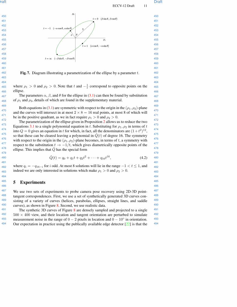
Fig. 7. Diagram illustrating a parametrization of the ellipse by a parameter t.

where ρ1 > 0 and ρ2 > 0. Note that t and −1t correspond to opposite points on the

ellipse.The parameters α, β, and θ for the ellipse in (3.1) can then be found by substitution

of ρ1 and ρ2, details of which are found in the supplementary material.

Both equations in (3.1) are symmetric with respect to the origin in the (ρ1, ρ2)-planeand the curves will intersect in at most 2× 8 = 16 real points, at most 8 of which willbe in the positive quadrant, as we in fact require ρ1 > 0 and ρ2 > 0.

The parametrization of the ellipse given in Proposition 2 allows us to reduce the twoEquations 3.1 to a single polynomial equation in t. Substituting for ρ1, ρ2 in terms of tinto Q = 0 gives an equation in t for which, in fact, all the denominators are (1+ t2)12,so that these can be cleared leaving a polynomial in Q(t) of degree 16. The symmetrywith respect to the origin in the (ρ1, ρ2)-plane becomes, in terms of t, a symmetry withrespect to the substitution t → −1/t, which gives diametrically opposite points of theellipse. This implies that Q has the special form

Q(t) = q0 + q1t+ q2t2 + · · ·+ q16t

16, (4.2)

where qi = −q16−i for i odd. At most 8 solutions will lie in the range −1 < t ≤ 1, andindeed we are only interested in solutions which make ρ1 > 0 and ρ2 > 0.

5 Experiments

We use two sets of experiments to probe camera pose recovery using 2D-3D point-tangent correspondences. First, we use a set of synthetically generated 3D curves con-sisting of a variety of curves (helices, parabolas, ellipses, straight lines, and saddlecurves), as shown in Figure 8. Second, we use realistic data.

The synthetic 3D curves of Figure 8 are densely sampled and projected to a single500 × 400 view, and their location and tangent orientation are perturbed to simulatemeasurement noise in the range of 0 − 2 pixels in location and 0 − 10◦ in orientation.Our expectation in practice using the publically available edge detector [22] is that the

495

496

497

498

499

500

501

502

503

504

505

506

507

508

509

510

511

512

513

514

515

516

517

518

519

520

521

522

523

524

525

526

527

528

529

530

531

532

533

534

535

536

537

538

539

495

496

497

498

499

500

501

502

503

504

505

506

507

508

509

510

511

512

513

514

515

516

517

518

519

520

521

522

523

524

525

526

527

528

529

530

531

532

533

534

535

536

537

538

539

ECCV#ECCV 2012

Accepted PaperDraft

ECCV#ECCV 2012

Accepted PaperDraft

12 ECCV-12 Draft

Fig. 8. Sample views of the synthetic dataset. Real datasets have also been used in ourexperiments, reported in further detail in the supplemental material.

edges can be found with subpixel accuracy and edge orientations are accurate to lessthan 5◦.

In order to simulate the intended application, pairs of 2D-3D point-tangent cor-respondences are selected in a RANSAC procedure from among 1000 veridical ones,to which 50% random spurious correspondences were added. The practical methoddiscussed in Section 4 is used to determine the pose of the camera (R, T ) inside theRANSAC loop. Each step takes 90ms in Matlab on a standard 2GHz dual-core laptop.What is most significant, however, is that only 17 runs are sufficient to get 99% proba-bility of hitting an outlier-free correspondence pair, or 32 runs for 99.99% probability.In practice more runs can easily be used depending on computational requirements. Toassess the output of the algorithm, we could have measured the error of the estimatedpose compared to the ground truth pose. However, what is more meaningful is the im-pact of the measured pose on the measured reprojection error, as commonly used in thefield to validate the output of RANSAC-based estimation. Since this is a controlled exper-iment, we measure final reprojection error not just to the inlier set, but to the entire poolof 1000 true correspondences. In practice, a bundle-adjustment would be run to refinethe pose estimate using all inliers, but we chose to report the raw errors without nonlin-ear least-squares refinement. The distribution of reprojection error is plotted for variouslevels of measurement noise, Figure 9. These plots show that the relative camera posecan be effectively determined for a viable range of measurement errors, specially sincethese results are typically optimized in practice through bundle adjustment. Additionalinformation can be found in the supplemental material.

Second, we use data from a real sequence, the “Capitol sequence”, which is a setof 256 frames covering a 90◦ helicopter fly-by from the Rhode Island State Capitol,Figure 2, using a High-Definition camera (1280 × 720). Intrinsic parameters were ini-tialized using the Matlab Calibration toolbox from J. Bouguet (future extension of thiswork would allow for an estimation of intrinsic parameters as well). The camera param-eters were obtained by running Bundler [1] essentially out-of-the-box, with calibrationaccuracy of 1.3px. In this setup, a pair of fully calibrated views are used to reconstructa 3D cloud of 30 edges from manual correspondences. Pairs of matches from 3D edgesto observed edges in novel views are used with RANSAC to compute the camera posewith respect to the frame of the 3D points, and measure reprojection error. One can theneither use multiple pairs or use bundle adjustment to improve the reprojection error re-

540

541

542

543

544

545

546

547

548

549

550

551

552

553

554

555

556

557

558

559

560

561

562

563

564

565

566

567

568

569

570

571

572

573

574

575

576

577

578

579

580

581

582

583

584

540

541

542

543

544

545

546

547

548

549

550

551

552

553

554

555

556

557

558

559

560

561

562

563

564

565

566

567

568

569

570

571

572

573

574

575

576

577

578

579

580

581

582

583

584

ECCV#ECCV 2012

Accepted PaperDraft

ECCV#ECCV 2012

Accepted PaperDraft

ECCV-12 Draft 13

0 1 2 3 4 5 6 70

0.05

0.1

0.15

0.2

0.25

0.3

0.35

0.4Error distribution for different noise levels

freq

uenc

y

reprojection error

∆

pos = 0.5, ∆θ = 0.5

∆pos

= 1, ∆θ = 0.5

∆pos

= 2, ∆θ = 0.5

∆pos

= 0.5, ∆θ = 1

∆pos

= 1, ∆θ = 1

∆pos

= 2, ∆θ = 1

∆pos

= 0.5, ∆θ = 5

∆pos

= 1, ∆θ = 5

∆pos

= 2, ∆θ = 5

∆pos

= 0.5, ∆θ = 10

∆pos

= 1, ∆θ = 10

∆pos

= 2, ∆θ = 10

Fig. 9. Distributions of reprojection error for synthetic data without running bundleadjustment, for increasing levels of positional and tangential perturbation in the mea-surements. Additional results are reported in the supplemental material.

sulting from our initial computation of relative pose. Figure 10 shows the reprojectionerror distribution of our method for a single point-tangent pair after RANSAC, beforeand after running bundle-adjustment, versus the dataset camera from bundler (which isbundle-adjusted), for the Capitol sequence. The proposed approach achieved an averageerror of 1.1px and 0.76px before and after a metric bundle adjustment, respectively, ascompared to 1.3px from Bundler. Additional information and results can be found inthe supplemental material.

0 0.5 1 1.5 2 2.5 3 3.50

0.05

0.1

0.15

0.2

0.25

0.3

0.35

freq

uenc

y

reprojection error

proposed method (w/o bundle adj.)bundlerproposed method (w/ bundle adj.)

Fig. 10. The reprojection error distribution for real data (Capitol sequence) using onlytwo point-tangents, before and after bundle adjustment. Additional results are re-ported in the supplemental material.

585

586

587

588

589

590

591

592

593

594

595

596

597

598

599

600

601

602

603

604

605

606

607

608

609

610

611

612

613

614

615

616

617

618

619

620

621

622

623

624

625

626

627

628

629

585

586

587

588

589

590

591

592

593

594

595

596

597

598

599

600

601

602

603

604

605

606

607

608

609

610

611

612

613

614

615

616

617

618

619

620

621

622

623

624

625

626

627

628

629

ECCV#ECCV 2012

Accepted PaperDraft

ECCV#ECCV 2012

Accepted PaperDraft

14 ECCV-12 Draft

6 Future Directions

The paper can be extended to consider the case when intrinsic parameters are unknown.Table 1 conjectures that four pairs of corresponding 3D-2D point-tangents are suffi-cient to solve this problem. Also, we have been working on the problem of determiningtrinocular relative pose from corresponding point-tangents across 3 views. We conjec-ture that three triplets of correspondences among the views are sufficient to establishrelative pose. This would allow for a complete curve-based structure from motion sys-tem starting from a set of images without any initial calibration.

References

1. S. Agarwal, N. Snavely, I. Simon, S. M. Seitz, and R. Szeliski. Building Rome in a day. InICCV ’09. 1, 12

2. N. Ayache and L. Lustman. Fast and reliable passive trinocular stereovision. In ICCV’87.3. M. Bujnak, Z. Kukelova, and T. Pajdla. A general solution to the p4p problem for camera

with unknown focal length. In CVPR’08. 74. R. Fabbri and B. B. Kimia. High-order differential geometry of curves for multiview recon-

struction and matching. In EMMCVPR’05. 45. R. Fabbri and B. B. Kimia. 3D curve sketch: Flexible curve-based stereo reconstruction and

calibration. In CVPR’10. 46. S. Finsterwalder and W. Scheufele. Das ruckwartseinschneiden im raum. Sebastian Finster-

walder zum 75, pages 86–100, 1937. 77. M. A. Fischler and R. C. Bolles. Random sample consensus: a paradigm for model fitting

with applications to image analysis and automated cartography. Commun. ACM, 24(6):381–395, 1981. 1, 6, 7

8. J. A. Grunert. Das pothenotische problem in erweiterter gestalt nebst Uber seine anwendun-gen in der geodasie. Archiv der fur Mathematik and Physik, 1:238–248, 1841. 7

9. R. M. Haralick, C.-N. Lee, K. Ottenberg, and M. Nolle. Review and analysis of solutions ofthe three point perspective pose estimation problem. IJCV, 13(3):331–356, 1994. 7

10. C. Harris and M. Stephens. A combined edge and corner detector. In Alvey Vision Confer-ence, 1988. 1

11. R. Hartley and A. Zisserman. Multiple View Geometry in Computer Vision. CambridgeUniversity Press, 2000. 1, 6

12. R. Horaud, B. Conio, O. Leboulleux, and B. Lacolle. An analytic solution for the p4p prob-lem. CVGIP, 47(1):33–44, 1989. 7

13. Z. Y. Hu and F. C. Wu. A note on the number of solutions of the noncoplanar p4p problem.PAMI, 24(4):550–555, 2002.

14. F. Kahl and A. Heyden. Using conic correspondence in two images to estimate the epipolargeometry. In ICCV’98. 3, 6

15. J. Y. Kaminski and A. Shashua. Multiple view geometry of general algebraic curves. IJCV,56(3):195–219, 2004. 3, 6

16. H. C. Longuet-Higgins. A computer algorithm for reconstructing a scene from two projec-tions. Nature, 293:133–135, 1981. 5

17. D. G. Lowe. Distinctive image features from scale-invariant keypoints. IJCV, 60(2):91–110,2004. 1

18. P. Moreels and P. Perona. Evaluation of features detectors and descriptors based on 3Dobjects. IJCV, 73(3):263–284, 2007. 2

19. J. Porrill and S. Pollard. Curve matching and stereo calibration. IVC, 9(1):45–50, 1991. 3, 5

630

631

632

633

634

635

636

637

638

639

640

641

642

643

644

645

646

647

648

649

650

651

652

653

654

655

656

657

658

659

660

661

662

663

664

665

666

667

668

669

670

671

672

673

674

630

631

632

633

634

635

636

637

638

639

640

641

642

643

644

645

646

647

648

649

650

651

652

653

654

655

656

657

658

659

660

661

662

663

664

665

666

667

668

669

670

671

672

673

674

ECCV#ECCV 2012

Accepted PaperDraft

ECCV#ECCV 2012

Accepted PaperDraft

ECCV-12 Draft 15

20. L. Robert and O. D. Faugeras. Curve-based stereo: figural continuity and curvature. InCVPR’91.

21. S. N. Sinha, M. Pollefeys, and L. McMillan. Camera network calibration from dynamicsilhouettes. In CVPR’04. 3, 6

22. A. Tamrakar and B. B. Kimia. No grouping left behind: From edges to curve fragments. InICCV ’07. 4, 11