DOES BEHAVIOURAL PLASTICITY CONTRIBUTE TO DIFFERENCES IN POPULATION GENETIC
STRUCTURE IN WILD RABBIT POPULATIONS IN ARID AND SEMI-ARID AUSTRALIA?
Mr Geoffrey Anthony de Zylva – B. App. Sc., Hons. School of Natural Resource Sciences Queensland University of Technology
Submitted for the degree of Doctor of Philosophy (Science), in 2007.

Keywords
Oryctolagus cuniculus
European Rabbit
Australia
DNA
mtDNA
microsatellite
behaviour
flexible behaviour
genetic variability
metapopulations
genetic bottleneck

Abstract
The European rabbit, Oryctolagus cuniculus, was introduced to Australia in 1859
and quickly became a significant vertebrate pest species in the country across a wide
distribution. In arid and semi-arid environments, rabbit populations exist as
metapopulations – undergoing frequent extinction recolonisation cycles. Previous
studies identified population genetic structuring at the regional level between arid
and semi-arid environments, and habitat heterogeneity was suggested as a possible
causal factor. For the most part, rabbit behaviour has been overlooked as a factor
that could contribute to explaining population genetic structure in arid and semi-arid
environments.
This study utilised a combination of genetic sampling techniques and a simulated
territorial intrusion approach to observing wild rabbit behaviour in arid and semi-
arid environments. The genetic component of the study compared population
samples from each region using four polymorphic microsatellite loci. The
behavioural component examined variation in the level of territoriality exhibited by
three study populations in the arid region towards rabbits of known versus unknown
origins (resident vs transgressor (simulating dispersal)).
A difference was observed in population genetic structure determined from nuclear
markers between arid and semi-arid regions, which supports findings of previous
research using mitochondrial DNA data in the same area. Additionally, differences
in aggressive response to known vs unknown rabbits were identified in parts of the
arid region, which together with the effects of habitat heterogeneity and connectivity
may explain the observed differences in population genetic structure.
Knowledge of behavioural plasticity and its effect on relative dispersal success and
population genetic structure may contribute to improved management and control of
feral rabbit populations at the regional level within Australia; and may assist with
conservation efforts in the species’ natural range in Europe.

Table of Contents CH1 - INTRODUCTION .......................................................................................................................... 1
DISPERSAL, HABITAT VARIABILITY, AND GENE FLOW ............................................................ 1 MODELLING GENE FLOW ......................................................................................................... 3 METAPOPULATIONS.................................................................................................................. 5 BEHAVIOURAL DIVERSITY AND GENETIC DETERMINATION..................................................... 10 GROUP LIVING, COOPERATION, AND SOCIALITY ..................................................................... 10 RESOURCE DEFENCE ............................................................................................................... 13 BEHAVIOURAL FLEXIBILITY..................................................................................................... 15 THE EUROPEAN RABBIT ........................................................................................................... 16
CH2 – EXPERIMENTAL DESIGN AND METHODOLOGY ......................................................................... 24 DESCRIPTION OF STUDY SITES ................................................................................................. 25 POPULATION SAMPLING ........................................................................................................... 27 GENETIC METHODS ................................................................................................................. 28 BEHAVIOURAL METHODS ........................................................................................................ 29
CH3 – GENETIC ANALYSIS .................................................................................................................. 32 MATERIALS AND METHODS ..................................................................................................... 33 DNA EXTRACTION................................................................................................................... 34 POLYMERASE CHAIN REACTION (PCR).................................................................................... 35 RESULTS................................................................................................................................... 41 DISCUSSION.............................................................................................................................. 50
CH4 – RABBIT BEHAVIOUR.................................................................................................................. 57 MATERIALS AND METHODS ..................................................................................................... 57 ANALYSIS METHODS – HABITAT CONDITIONS ......................................................................... 60 ANALYSIS METHODS – BEHAVIOUR ........................................................................................ 61 RESULTS................................................................................................................................... 64 DISCUSSION………………………………………………………………………………… 103
CH5 - GENERAL DISCUSSION.............................................................................................................111 POPULATION GENETICS..........................................................................................................111 BEHAVIOURAL ECOLOGY .......................................................................................................114 PEST MANAGEMENT ISSUES ...................................................................................................119 FUTURE DIRECTIONS OF RESEARCH AND CONCLUSION..........................................................123
APPENDIX 1 – LIST OF ALL RABBIT BEHAVIOURS ...............................................................................125 BIBLIOGRAPHY ..................................................................................................................................127

List of Tables and Figures FIGURE 1.1 - TYPES OF METAPOPULATION ............................................................................................ 6 FIGURE 2.1 – AREAS OF STUDY ............................................................................................................ 27 TABLE 3.1 – MICROSATELLITE PRIMERS ............................................................................................... 35 TABLE 3.2 – PCR AND ELECTROPHORESIS CONDITIONS (TA = ANNEALING TEMPERATURE)................... 38 TABLE 3.3 – POPULATION SAMPLE SIZES AT EACH LOCUS ..................................................................... 39 TABLE 3.4 – NUMBER OF ALLELES PER LOCUS PER POPULATION ........................................................... 41 TABLE 3.5 – MEAN ALLELIC STATISTICS ACROSS ALL LOCI FOR EACH POPULATION.............................. 42 TABLE 3.6 – SIGNIFICANT GENIC DIFFERENTIATION FOR POPULATION PAIRS ACROSS ALL LOCI ............ 43 TABLE 3.7 – MATRIX OF SIGNIFICANT GENIC DIFFERENTIATION BETWEEN POPULATION PAIRS ............. 44 TABLE 3.8 – PAIRWISE POPULATION FST VALUES.................................................................................. 45 TABLE 3.9 – SIGNIFICANCE OF PAIRWISE POPULATION FST VALUES...................................................... 45 FIGURE 3.1 – SORTED MEAN FIS............................................................................................................ 46 TABLE 3.10 – AMOVA SUMMARY TABLE ............................................................................................ 47 FIGURE 3.2 – AMOVA SUMMARY PIE CHART...................................................................................... 47 FIGURE 3.3 – RANDOMISATION OF PHIPT ............................................................................................. 48 FIGURE 3.4 - UPGMA TREE FOR NEI SIMILARITY MATRIX .................................................................... 49 TABLE 3.11 – SPECIES WITH REDUCED GENETIC DIVERSITY .................................................................. 51 TABLE 4.1 – SITE LOCATIONS................................................................................................................ 58 FIGURE 4.1 – VISION FIELD OF VIDEO CAMERA ..................................................................................... 60 TABLE 4.2 – BEHAVIOUR OBSERVED ON VIDEO..................................................................................... 62 TABLE 4.3 - WARREN COUNT DATA ..................................................................................................... 64 FIGURE 4.2 – 2001 RABBIT WEIGHT V SEX (TOTAL CAPTURES) ............................................................ 65 FIGURE 4.3 – 2002 RABBIT WEIGHT V SEX (TOTAL CAPTURES) ............................................................ 66 FIGURE 4.4 – MEAN DECOY WEIGHT .................................................................................................... 67 TABLE 4.4 – MEAN PERCENTAGE COVER............................................................................................... 67 FIGURE 4.5 – MEAN PERCENT COVER COMPARISON BETWEEN YEARS SITE 1 ........................................ 68 FIGURE 4.6 – MEAN PERCENT COVER COMPARISON BETWEEN YEARS SITE 2 ........................................ 69 FIGURE 4.7 – MEAN PERCENT COVER COMPARISON BETWEEN YEARS SITE 3 ........................................ 70 FIGURE 4.8 – SCATTERPLOT OF TOTAL BEHAVIOUR VS NUMBER OF RABBITS ...................................... 72 FIGURE 4.9 – MEAN PLOT OF SUM BEHAVIOUR PER RABBIT PER HOUR................................................ 73 FIGURE 4.10 – AGGRESSIVE BEHAVIOUR SITE 1 CONTROL 2001........................................................... 75 FIGURE 4.11 – AGGRESSIVE BEHAVIOUR SITE 1 EXPERIMENTAL 2001.................................................. 76 FIGURE 4.12 – AGGRESSIVE BEHAVIOUR SITE 2 CONTROL 2001........................................................... 77 FIGURE 4.13 – AGGRESSIVE BEHAVIOUR SITE 2 EXPERIMENTAL 2001.................................................. 78 FIGURE 4.14 – AGGRESSIVE BEHAVIOUR SITE 3 CONTROL 2001........................................................... 79 FIGURE 4.15 – AGGRESSIVE BEHAVIOUR SITE 3 EXPERIMENTAL 2001.................................................. 80 FIGURE 4.16 – AGGRESSIVE BEHAVIOUR SITE 1 CONTROL 2002........................................................... 81 FIGURE 4.17 – AGGRESSIVE BEHAVIOUR SITE 1 EXPERIMENTAL 2002.................................................. 82 FIGURE 4.18 – AGGRESSIVE BEHAVIOUR SITE 2 EXPERIMENTAL 2002.................................................. 83 FIGURE 4.19 – AGGRESSIVE BEHAVIOUR SITE 1 CONTROL 2002........................................................... 84 FIGURE 4.20 – AGGRESSIVE BEHAVIOUR SITE 2 EXPERIMENTAL 2002.................................................. 85 FIGURE 4.21 – 10MIN INTERVAL PLOT SITE 1 2001 ............................................................................... 87 FIGURE 4.22 – 10MIN INTERVAL PLOT SITE 2 2001 ............................................................................... 88 FIGURE 4.23 – 10MIN INTERVAL PLOT SITE 3 2001 ............................................................................... 89 FIGURE 4.24 – 10MIN INTERVAL PLOT SITE 1 2002 ............................................................................... 90 FIGURE 4.25 – 10MIN INTERVAL PLOT SITE 2 2002 ............................................................................... 91 FIGURE 4.26 – 10MIN INTERVAL PLOT SITE 3 2001 ............................................................................... 92 TABLE 4.5 – T TEST SITE 1 CONTROL V EXPERIMENTAL 2001 .............................................................. 93 TABLE 4.6 – T TEST SITE 2 CONTROL V EXPERIMENTAL 2001 .............................................................. 93 TABLE 4.7 – T TEST SITE 3 CONTROL V EXPERIMENTAL 2001 .............................................................. 94 TABLE 4.8 – T TEST SITE 1 CONTROL V EXPERIMENTAL 2002 .............................................................. 94 TABLE 4.9 – T TEST SITE 3 CONTROL V EXPERIMENTAL 2002 .............................................................. 94 TABLE 4.10 – ANOVA ACROSS ALL SITES CONTROL DATA 2001 ......................................................... 95 TABLE 4.11 – ANOVA ACROSS ALL SITES EXPERIMENTAL DATA 2001 ................................................ 96 TABLE 4.12 – T TEST SITE 1 V SITE 3 CONTROL DATA 2002.................................................................. 96 TABLE 4.13 – T TEST SITE 1 V SITE 3 EXPERIMENTAL DATA 2002 ........................................................ 97 TABLE 4.14 – T TEST YEAR COMPARISON AT SITE 1 ............................................................................ 98 TABLE 4.15 – T TEST YEAR COMPARISON AT SITE 3 ............................................................................ 98 FIGURE 4.27 – GENERAL LINEAR MODELLING...................................................................................... 99 TABLE 4.16 – PERCENTAGE OF TOTAL BEHAVIOUR OCCURING IN FIRST 15MINS.................................101 TABLE 4.17 – PROPORTION OF AGGRESSIVE BEHAVIOUR IN FIRST 15 MINS ..........................................101 FIGURE 5.1 – BREAKDOWN OF SOCIAL SYSTEMS DUE TO VARIABLE RESOURCES..................................116 FIGURE 5.2 – RABBIT CALCI VIRUS RELEASE, MITCHELL, 1996............................................................122

STATEMENT OF ORIGINAL AUTHORSHIP
The work contained in this thesis has not been previously submitted for a degree or diploma at any other higher education institution. To the best of my knowledge and belief, the thesis contains no material previously published or written by another person except where due reference is made. Signature:_______________ Date:___________________

ACKNOWLEDGEMENTS This thesis would not have been possible without the support of Peter Mather and John Wilson. Thankyou for your advice, encouragement, and inspirational enthusiasm for ecology. I also wish to recognise the financial support from The School of Natural Resource Sciences QUT, and the Federal Government. Many thanks also to Dave Berman and his team of “Bulloo Warriors” from the Queensland Department of Natural Resources, particularly Michael Brennan, Craig Hunter, Peter Elsworth, and John Conroy – I would be buried in the desert if it weren’t for you blokes. Thankyou to Stanbroke Pastoral Company for access to Bulloo Downs, and thanks to Geoff and Wendy Murrell and all the staff of Bulloo Downs for your hospitality during my field trips. To the various landholders in the Mitchell Region, thankyou for access to your properties during my various pilot trips – I hope the rabbits stay away for many years to come. I owe a huge debt of thanks to those who volunteered their time to drive to the middle of Australia and chase rabbits: Ben de Zylva (who enjoyed the first trip so much he came back for more), Alison Crawford, and Alex Wilson. Our trips to Bulloo Downs would not have been possible without the logistical support team: Jo Chambers, Peter Prentis, and Stephen Craig-Smith – thanks for driving to Cunnamulla. This project would not have been possible without the cast of thousands from QUT, from the admin support to the radiation lab. Nat and Juanita (thanks for the help in the lab), Craig and Danny (thanks for sharing an office with me), and everyone at the Campus Club (thanks for the 12 hour lunches). Special thanks to Grant Hamilton and his efforts to “Show me the bunnies!” Let this thesis serve as an example of “what not to do” – the external factors such as drought and disease necessitated much variation to the original experimental design, to the point that resulted in a fairly limp dataset, containing far too many assumptions. If future students read this, please make sure you have the ability to collect enough data to rigorously test your theory. Check your field sites early, and if it looks like you can’t get the data – find another way to test your theory – or even change your topic altogether. Finally, thankyou to Rebecca, without your help I wouldn’t have made it this far.


Chapter 1 Introduction
Introduction
In many animal species, social behaviour can influence many aspects of life history
characteristics. The interaction, however, is bi-directional in the sense that social
behaviour can be influenced by a species’ characteristics in addition to external
environmental factors. The idea that behaviour patterns are inflexible within species
has been challenged by new research into social systems and genetics. This review
aims to explore the idea that a species' social structure can be influenced by different
environmental factors that it experiences.
Dispersal, Habitat Variability, And Gene Flow
Organisms that live in groups must ultimately decide whether to stay in the natal
territory or to disperse into new areas. Many factors influence the potential for
individuals to disperse successfully, not the least of which, is social organisation. If
an individual is of low rank in a social hierarchy, then dispersal to a new territory
may be a good option if the cost of dispersing is offset by the benefits gained by
reaching a new territory. Dispersal is only effective however, if an individual is able
to survive and reproduce in the new habitat. Three main types of dispersal have been
described (Krebs 1994). Diffusion is the gradual movement of a population across
hospitable terrain that occurs over several generations. Jump dispersal occurs when
individuals move large distances in a single event, usually across areas of
unfavourable habitat. Species introduced to non native areas through human
intervention can be viewed as an assisted form of jump dispersal. Secular dispersal is
a diffusion event that occurs over geological time and usually involves an
evolutionary change in the species across a specified time period; it can also be
associated with continental drift.
Habitat quality has the potential to affect both the social organisation of a species, its
dispersal dynamics, and the interrelationships between the two. A habitat that is
temporally and spatially stable is likely to be used in a different manner to one that is
dynamic. In a study of the red squirrel, Sciurus vulgaris, Lurzs et al. (1997)
examined the effect of habitat variability (temporal and spatial) on dispersal. They
studied squirrel dispersal patterns in a stable habitat with a reliable food supply, and
1

Chapter 1 Introduction
a variable habitat with temporal and spatial differences in food availability. In both
habitats, they observed male-biased dispersal in spring and female-biased dispersal in
autumn. More adults dispersed however, in the variable (66%) than in the stable
(31%) habitat. Large differences were also evident in the extent of site fidelity
between the two squirrel populations. Food availability was the main factor that
affected female dispersal. In contrast, male dispersal was influenced by the
distribution of females with male site fidelity high in the stable habitat, whereas
males tracked the movement of females in the variable habitat. This most likely
occurs because the stable habitat has sufficient resources to satisfy female needs.
Lurz's et al. (1997) data on squirrels suggest that female dispersal patterns are an
adaptive response to the spatial and temporal predictability of food resources.
Dispersal of individuals into potentially new habitat or territory that leads to effective
reproduction can result in gene flow. Different dispersal strategies can therefore lead
to different population genetic structures that are consequences of different
behaviour patterns. Dispersal or migration alone does not constitute gene flow - there
must also be an exchange or transfer of genetic material i.e. reproduction. Gene flow
(or a lack thereof) can lead to population structuring, which is defined as differences
in genetic variation among constituent parts of a species’ natural range, provided the
effect is not counteracted by other evolutionary processes such as a mutation, natural
selection or genetic drift. Gene flow is a major factor which influences population
structure because it determines the extent to which each local population of a species
acts as an independent evolutionary unit. If a large amount of gene flow occurs
among local populations, then the collection of populations evolve together; but if
there is little gene flow each population will tend to evolve independently (Slatkin
1994). A number of theoretical models have been developed which describe gene
flow and its potential effects on population genetic structure.
Modelling Gene Flow
The simplest models are based on the island model of migration which was first
proposed by Wright (1931). In this model, a species' distribution consists of discrete
populations that are geographically separated and are assumed to be large enough
such that genetic drift can be ignored as a population structuring process. Migration
2

Chapter 1 Introduction
is assumed to occur between population islands as a process in which the allele
frequency of the migrants is equivalent to that of the total population and therefore
the amount of migration is measured as the probability that a randomly chosen allele
in any sub-population comes from a migrant (Hartl and Clark 1997).
Two alternative models were developed that address population structure in
continuous rather than discrete population systems: 'Isolation by distance' models,
and 'Stepping stone' models. Sewall Wright was also responsible for the early work
on isolation by distance. The theory is based on the premise that if, in the continuous
distribution of a population, migration of individuals and subsequent interbreeding is
restricted to short distances due to short range dispersal; then remote populations
may be differentiated because of the distance among them (Wright 1943).
The concept of a species' range being large enough such that colonies develop and
exchange genetic information through migration was developed by Kimura and
Weiss (1964). They proposed three types of stepping stone model with increasing
degrees of complexity referred to as 1, 2, and 3 dimensional models.
A one dimensional model is where the colonies are located in a linear fashion.
Migration can only occur between adjacent colonies, that is, for each generation an
individual can migrate 'one step' in either direction. For the other two models, the
array of colonies will increase. The two dimensional model assumes a rectangular
arrangement of colonies, therefore an individual can migrate in four directions. The
third dimensional model introduces a cubic system in which migration can occur in
six directions. It is important to note that the 3rd dimension does not necessarily have
to be of a spatial or habitat capacity, it may simply refer to an attribute of the species
that enables greater variety in life style. Social rank is an example of one factor that
may provide a third dimension to population structure.
The development of methods for estimating gene flow occurred as a corollary to the
theoretical work that developed the models. Direct estimation methods are based on
experiments or field observation which gather measurements of dispersal distances.
The distance estimates can be converted into estimated gene flow based on the
assumption that migrant individuals have the same probability of reproductive
3

Chapter 1 Introduction
success as do residents. Indirect methods, however, are based on mathematical
models which explain interactions of gene flow and other forces to predict how much
gene flow must have been occurring to explain the observed patterns (Slatkin 1994).
Wrights FST statistic is the best known of these methods; it is a measure of the
correlation between genes in a sub-population relative to the entire population
(Wright 1951). The model states that in an island model at equilibrium,
FST = 1/1 + 4Nm where N = the effective population size, and m = immigration rate.
There is no way to gain a separate estimate for the terms N and m, however, by
solving for Nm the formula is transformed to Nm = 1/4 (1/ FST - 1). FST can be
calculated easily from allele frequency data. By solving the equation, one gains an
estimate of gene flow for the population under study.
Distinct advantages and disadvantages are associated with the direct and indirect
methods of gene flow estimation, which are discussed by Slatkin (1994). Direct
estimates can reveal certain aspects of the dispersal mode such as the life stage most
common for dispersal, and the environmental conditions most conducive to dispersal.
The disadvantage of the direct methods is that they are limited by the size of the
project, and it can be difficult to gather information regarding any long distance
dispersal or dispersal under abnormal environmental conditions. Indirect methods are
able to incorporate any effects of variation in dispersal and average out the
differences over time. The major disadvantage however, is that the methods rely on
assumptions regarding allele frequencies, and these assumptions cannot always be
tested independently.
The use of indirect methods to measure dispersal, and in particular, to estimate gene
flow using Nm has been accepted practise for many years. More recently however,
conjecture has grown regarding the validity of the formula. Whitlock and McCauley
(1999) argue that in many cases FST does not equate to the formula 1/(4Nm + 1),
because the formula is based on several assumptions that are violated in most natural
systems. The five critical assumptions are:
1) The alleles at the loci are selectively neutral and are not linked to selected loci.
2) The rate of mutation is not high relative to the rate of migration.
3) All populations are created equal, with a constant number of individuals and
equal contributions to the migrant pool.
4

Chapter 1 Introduction
4) Migration is random (no spatial structure).
5) The system is in equilibrium between migration and genetic drift.
Measurement of genetic variation from genetic data is a valid use of FST, however, it
is clear that estimates of dispersal and gene flow based on F statistics should be
viewed with care. Estimates may be correct within a few orders of magnitude, and
should be performed only in situations when the biological question depends on
estimating migration rates among populations where 'errors' associated with the
estimate can be relatively large (Whitlock and McCauley 1999).
Metapopulations
Following on from the ideas on dispersal developed with Island and Stepping-Stone
models, came the concept of metapopulations. The term itself is used to define a set
of local populations that interact via individuals moving among populations (i.e.
dispersing). The characteristic feature of a metapopulation is that local populations
are dynamic and will undergo phases of extinction, and subsequent recolonisation
from other populations within the system; this is also referred to as turnover. Several
kinds of metapopulation were characterised and summarised in Harrison (1991)
(figure 1.1).
5

Chapter 1 Introduction
Closed circles represent habitat patches; filled = occupied, unfilled = vacant. Dashed lines show the boundaries of populations. Arrows indicate migration (colonisation). A. Levins-type metapopulation. B. Mainland-island/source-sink metapopulation. C. ‘Patchy population’. D. Non-equilibrium metapopulation. E. An intermediate combination of B and C.
Figure 1.1 Types of Metapopulations (reproduced from Harrison, 1991)
The Levin's (1969) model of metapopulations (figure 1.1A) was the first step in
developing theories behind newer models. It is based on the scenario where a set of
conspecific populations exists in a balance, at the regional level, between extinction
and colonisation. This model most closely resembles the island and stepping stone
models of migration. Mainland-island and Source-sink metapopulations (figure 1.1B)
6

Chapter 1 Introduction
occur when there is one large central patch that is resistant to extinction, with
peripheral patches that undergo periods of extinction and subsequent recolonisation
by migrants from the main patch. There is a distinct difference however, between
these types of metapopulations with respect to the outlying patches. Island habitats
are simply smaller versions of mainland habitats, whereas sinks are qualitatively
different from sources, being unsuitable in some way for survival and reproduction
(Harrison 1991). This type of metapopulation has also been referred to as a 'Core-
satellite system' (Hanski and Gilpin, 1991).
The patchy population (figure 1.1C) describes systems where habitat patches exhibit
spatial and temporal variation, however, there are also large amounts of dispersal
among patches, which effectively makes the group of populations a single interacting
unit. There is little opportunity for extinction to occur in a system like this because of
the high rates of dispersal. A non-equilibrium population (figure 1.1D) is
diagrammatically similar to the basic Levin's model (figure 1.1A) except that the
recolonisation process does not occur. If there is a lack of migration (recolonisation),
then when a patch becomes extinct, it will remain so. It represents a population
system of species in regional decline.
The main factors affecting localised extinction rates are usually stochastic in nature,
and include demographic, genetic, environmental, and catastrophic processes/events
(Shaffer 1981; Harrison 1991). Random changes in birth and death rates represent
demographic factors. These are most likely to have the greatest effect on small
populations or those in regional decline that are below a population size threshold
(Ebenhard 1991). Obviously, threshold levels will vary among species. Genetic
stochasticity concerns the loss of heterozygosity through drift effects and inbreeding
– the net result being a reduction in fitness, and increased probability of extinction. A
genetic effect, like a demographic effect, is more likely to occur in small populations,
however, it will definitely be more pronounced in a population that is newly small,
and is not conditioned to undergoing periods of population flux.
Environmental stochasticity and catastrophes are probably the most important causes
of local extinction because they can affect populations of varying sizes (Harrison
1991). Variations in environmental characters such as food availability and weather
7

Chapter 1 Introduction
conditions may affect the entire range of patches in a region, yet not all populations
are likely to go extinct. This observation led to the idea that certain patches are
effectively refuges that enable survival through adverse environmental conditions;
either by providing basal nutritional requirements or by providing better quality
shelter sites that, in some species, will facilitate a period of torpor until conditions
are more conducive to reproduction and dispersal (Harrison, 1991). In some
instances, larger patches will be better suited for use as refugia simply due to size
and ability to ‘absorb’ adverse conditions better than smaller patches – this would be
commonly observed in mainland-island metapopulations. Catastrophic events such as
flood, drought, and fire usually cause widespread extinctions in metapopulations.
While survival may be higher in larger patches, this will depend to a large extent on
the species in question and the nature of the catastrophe.
A metapopulation can persist only when colonisation follows extinction events.
Colonisation can be defined as starting with the arrival of a propagule (the migrants)
and ending when the extinction probability of the population no longer depends on
the initial state of the propagule (Ebenhard 1991). While the process could be viewed
simply as dispersal from an occupied patch, the migrant individuals must move
through inhospitable habitat in order to colonise the extinct patch. This process will
present its own set of problems. The success of the propagule will depend on the
probability of finding a suitable patch, and effectively reproducing once there.
Differences in dispersal rates among sex and age classes are most common in
polygamous species and in long-lived species with many litters per female (Hansson
1991). Other important observations on dispersal made by Hansson (1991) are that
dispersal distances appear to be longer in poor environments and habitat specialists
are more affected by boundaries than habitat generalists. Thus the ability of a species
to survive the dispersal phase through harsh environments will enhance its ability to
function as a metapopulation. Individuals in the colonised patch will have a higher
probability of extinction in the new habitat, than if they dispersed within the natal
patch. Ebenhard (1991) presents data which suggests the best colonisers will be large
propagules with potential for rapid increase in variable habitats or with a low
mortality in stable habitats. Dispersing propagules may also reach patches with
extant populations, and while this is not considered a colonisation event in the
strictest terms, it does have some important ramifications for metapopulation
8

Chapter 1 Introduction
dynamics. The migrant individuals may offer the opportunity for gene flow to occur,
possibly reducing the chance of inbreeding and any associated deleterious effects
(Gilpin, 1987). Migrants arriving successfully in an occupied patch may also be of
benefit to the local population if it is in decline, for whatever reason, by boosting the
species abundance in the patch – an occurrence referred to as the 'rescue effect'
(Hanski, 1991). An alternative scenario, however is that the migrant individuals may
not integrate with the local population at all, and instead develop their own
independent breeding group which would be detrimental to the original declining
population.
Severe fluctuations in population size (where periods of small population sizes
occur) can reduce allelic diversity and heterozygosity levels in a population. It is an
effect commonly referred to as a genetic bottleneck (Hedrick 1999). Elephant seals
and African cheetahs are two examples of species which have low levels of genetic
diversity that can be explained by historical bottlenecks (Bonnell and Selander 1974;
O'Brien et al. 1987). Random genetic drift caused by migration of a few individuals
to a new patch from an established subpopulation can create a bottleneck known as a
founder effect (Hartl 1997). The classic examples of founder effects occur in
instances where species have been introduced (translocated) through human activities
into completely new habitats (eg. Bufo marinus, the cane toad, and Oryctolagus
cuniculus, the European rabbit in Australia).
9

Chapter 1 Introduction
Behavioural Diversity And Genetic Determination
Individual differences in behaviour can influence differences in dispersal strategy.
Dispersal, however, represents only one type of behaviour and there are a great
diversity of potential behaviours, many of which have a genetic component.
Evidence for the genetic determination of dispersal/movement behaviour is
widespread, one example occurs in fruit fly larvae. The larvae occur either as
‘rovers’, which move a long way to find food, or ‘sitters’, which forage in a more
restricted area; the polymorphism is determined by alleles at a cyclic GMP-
dependent protein kinase gene (Partridge and Sgro 1998). It is clear that selection is
able to act upon genes controlling behaviour; in the case of the fruit fly larvae, where
‘rovers’ may have an advantage in crowded populations, ‘sitters’ may have an
advantage in low density populations. Studies on the genetics of behaviour led
Alcock (1984) to the following generalisations:
1. Single allelic differences can influence behavioural differences among
individuals.
2. Artificial selection for certain behavioural traits can be highly effective in
altering the behaviour of a population over time.
3. Physiological effects that are determined by genetic differences among
individuals are responsible for their distinctive behavioural characteristics.
4. Differences in the genetic and physiological characteristics of populations of the
same species may be related to variation in ecological pressures operating in
different areas.
The fact that selection can act on genes which determine behaviour, therefore means
that behaviour can evolve through this process, like any other trait which is under
natural selection.
Group Living, Cooperation, And Sociality
While evolution of social behaviour has been studied extensively, much of the
earliest work focused on how evolution of behavioural strategies were of benefit to
the group. Tinbergen (1964) suggested that groups of 'capable' individuals survive,
while those containing inferior individuals do not, and therefore cannot reproduce
effectively. He was essentially arguing for group selection influencing the fitness of
10

Chapter 1 Introduction
individuals. This theory was opposed by Williams (1966) who suggested that clutch
size and many social interactions enhance individual fitness. Williams argued social
behaviours evolved for the benefit of the individual, not the group. Altruistic
behaviours however, which involve the act of sacrificing ones personal fitness for
the benefit of others, does not appear to fit his argument easily. Hamilton (1964a,b),
in discussing the evolution of altruism, raised the issue of inclusive fitness when he
suggested that individuals can pass copies of their genes to future generations by
assisting the reproduction of close relatives (indirect fitness) as well as via their own
reproductive efforts (direct fitness). Hamilton described a model that allowed for
interactions between relatives which affect fitness. Species which act 'altruistically'
may evolve behaviours so that individuals maximise their inclusive fitness and this
implies a limited restraint on selfish competitive and self-sacrificing behaviours
(Hamilton 1964a,b). Hamilton’s theory can more easily explain the evolution of
altruistic behavioural patterns such as cooperative breeding and coloniality.
The bell minor, Manorina melanophrys, is an example of a species that breeds
cooperatively. Individuals have never been observed breeding unassisted and
individual helpers, even breeders, often give aid to a number of breeding pairs within
a breeding season (Painter et al. 2000). The species has a multi-tiered behavioural
and social organisation, which was observed in studies by Clarke (1984, 1989) and
Clarke & Fitzgerald (1994). There are three levels of social organisation: colony,
coterie, and the nest contingent. The colony is a geographically discrete collection of
up to 200 individuals that communally defend an area against both inter- and
intraspecific avian competitors. The coterie is a group within the colony that contains
one or more breeding pairs. While helpers may aid more than one pair within a
coterie, they do not interact with members from other coteries except in territorial
defense. The third level of social organisation is the nest contingent, which consists
of individuals that assist at the nest as well as the breeding pair(s). Painter et al.
(2000) found (using microsatellite analysis) significant differences between coteries
in a high density colony, which resulted from related individuals associating
preferentially with each other. They also showed that individuals helping at the nest
were close relatives of the breeders, thus supporting models of kin selection for the
evolution of altruism in this bird. The classic examples of kin selection, however,
occur in eusocial insects including bees, wasps, and ants. In eusocial societies, a
11

Chapter 1 Introduction
queen produces all the offspring, and an army of sterile workers that share most of
their genes in common with their siblings. The evolution of eusocial systems is
complicated however, by ploidy differences between the two sexes. Females are
diploid and males haploid, a situation which changes the argument about altruism
when genetic relationships between offspring and parents are considered.
The main reason for the evolution of social behaviour is that natural selection has
influenced the frequencies of genes that give rise to such displays. Some species will
have certain evolutionary adaptations that favour the adoption of sociality while
others will not. Ultimately, it is natural selection or genetic drift acting on random
mutations that cause social behaviour to evolve in species, and consequently there
are several advantages and disadvantages. Through the selective process each
condition will affect individual fitness in a different manner for each species.
Costs and benefits of social behaviour (from Alcock, 1984)
Benefits:
Reduction in predator pressure by better detection and/or repulsion.
Improved foraging efficiency for large game or spatially and temporally clumped
resources.
Better defence of limited resources (space and food) against other groups of
conspecifics.
Enhanced care of offspring through communal feeding and protection.
Costs:
• Competition within the group for food, mates, nest sites and materials.
• Risk of infection by contagious diseases and parasites.
• Exploitation of parental care by conspecifics.
• Increased risk that conspecifics will kill progeny.
For species that have evolved solitary lifestyles, the costs may be greater than any
benefits gained from social living. Conversely, for species that live in social
communities the costs may be equalised or bettered by the benefits of the behaviour.
A good example occurs in two closely related species of freshwater fish, Lepomis
12

Chapter 1 Introduction
macrochris and Lepomis gibbosus (bluegill and pumpkinseed sunfish), studied by
(Gross and MacMillan 1981). The bluegill sunfish exhibits social behaviour during
the breeding season when males construct nests close together to form a colony.
Formation of the colony results in reduced pressure from the primary predators of
their eggs, which are catfish and snails, because males cooperate in colony defense.
The advantage of sociality to the bluegill is reduced by factors such as conspecific
interference and predation of eggs, as well as disease (fungi) that can spread through
dense colonies. The pumpkinseed sunfish however, lives a solitary life due in part to
the evolution of large, strong mouthparts designed for crushing snails and deterring
other potential predators. Colonial nesting is not advantageous to the pumpkinseed
sunfish because predation is not as great a problem as it is for the bluegill sunfish.
Resource Defence
The use of caches (food storing) usually occurs in species that exhibit territorial
behaviour and the act of creating the cache is a potentially costly exercise. Roberts
(1979) argued that adaptations are likely to arise that will reduce costs and/or
increase benefits - and that territoriality is one such adaptation in this sense because
it reduces the amount of competitors that are able to gain access to stored resources.
When food is clumped spatially, aggressiveness can be expected to increase because
the cost of defending an area is small compared to the benefit of access to a large
share of the resource (Grant 1993). If food is clumped temporally, aggression levels
may be expected to fall because any time spent defending is simultaneously time
away from resource utilisation (Trivers 1972; Wells 1977; Robb and Grant 1998).
The mountain lion (Puma concolor), is one organism in which intraspecific
aggression is known to occur (Pierce et al. 1998). In this instance the food resource is
not clumped temporally, but instead the social class of females with kittens utilise the
resource at an earlier time than other social classes. Adult females usually have
overlapping home ranges that also overlap within the range of one or more males.
Females tend to reduce confrontations through a system of mutual avoidance,
however, it is not uncommon for males to kill other males, females, juveniles and
kittens (Seindensticker et al. 1973). As mountain lions are known to cache food and
have overlapping home ranges, Pierce et. al. (1998) suggest that females with kittens
that visit the cached prey at different times to the other social classes, could obtain
13

Chapter 1 Introduction
fitness benefits by further minimising the probability of contact with other mountain
lions. In this example, one could argue that the resource is clumped spatially, in the
cache location, however, aggressiveness does not increase (with respect to the
suckling females) due to the differential timing of feeding events.
In some cases, resource clumping (spatially) is the result of an organism actively
caching food. Smith and Reichman (1984) in their review of caching by birds and
mammals limited their discussion to the movement of potential food from one
location to another for consumption at a later date. Not all species cache food, those
that do are found predominantly in temperate rather than tropical areas. This is most
likely because food resources are more predictable temporally in tropical areas which
probably negates the need to cache food. The high temperatures and humidity of a
tropical environment may also promote spoiling of cached food, which reduces the
efficiency of the method as a means of survival through unfavourable conditions
(Smith and Reichman 1984). Species that are known to cache food, will do so in one
of two ways. They can create a horde cache, or many scatter caches. The evolution of
caching behaviour is a method of resource defence. Horde caches can be effective
methods of food storage when the individual is able to defend the cache from
competitors. If an active defence is not feasible however, then scattering several
caches across a home range can be a viable alternative provided the organism is
capable of remembering all cache locations. Many species have been shown to
possess the ability to remember the location of caches and distinguish which are used
and unused (Wrazen and Wrazen 1982; Sherry 1984; Smith and Reichman 1984).
As mentioned above, resource defence through territoriality is one of the factors that
is considered to have led to the evolution of group living in many species. The cost
of sharing the resource within a territory with conspecifics is balanced by the benefits
gained from exclusive access to the resource, whether it is cached or distributed
naturally. Furthermore, the benefits in terms of fitness and selection are increased if
the members of the group belong to the same deme. If an individual is not dominant
or not producing offspring, then by participating in group behaviour, it may
contribute to the survival and breeding success of closely related individuals and thus
increase the likelihood of a small percentage of its own genes being passed to the
next generation through relatives (inclusive fitness).
14

Chapter 1 Introduction
Territory defence, however, is not the only contribution to group living that an
individual can make. Other activities that benefit the collective include predator
avoidance/warnings, collection of food, and rearing of young. If the group consists of
individuals that are not related, there may still be benefits associated with
participating in predator warnings and avoidance, as well as access to communal
food resources. Social hierarchies develop as a consequence of group living, and
therefore many species that live in groups (though not all) exhibit this structure to
varying degrees. In a study of the crane, Grus grus, foraging in cereal farmland
Alonso et al. (1995) found that birds left more resource-rich patches earlier than
expected and at higher intake rates than in poor patches, although they stayed longer
when in larger flocks. The results suggest that cranes may change their foraging
behaviour according to their expected energy balance. In this instance, cranes benefit
from group association by gaining greater food intake, and better avoidance of
predators.
Behavioural Flexibility
Behaviour can be modified by the environment, and clear-cut relationships between
energy requirements, resource distribution, and social systems can often be
demonstrated (Pough et al. 1989). An animal with a large mass will have much
greater energy requirements relative to a small animal. To obtain the necessary
resources, the animal may have to search widely across their home range - the area
in which they live to find their food and shelter. One might expect to find the size of
home range correlated with size/mass of an animal, but this does not take into
account the possibility of habitat patchiness. An animal may utilise a resource that
occurs in an uneven distribution, if so, then the size of the home range will be a
reflection of the quality of the habitat (in terms of the resource in question). Forest
duikers (small African antelope) have been shown to be more active in habitats of
high quality, although differences in home range have been observed between the
blue and red species (Bowland and Perrin 1995). Bowland (1995) found that core
areas in the home range of both duiker species were usually associated with bed sites.
Blue duiker home ranges and core areas however, were fixed year round with no
overlap between neighbours, while home ranges and core areas of red duikers
15
Chapter 1 Introduction
overlapped extensively. Temporal separation in red duikers is suggested between
some individuals and not others, which means there may be occasions where red
duiker individuals come in contact whilst using the overlapping home range. If
contact is occurring between red duikers, then passive or tolerance behaviour may
occur - which may manifest itself simply as non-recognition (ignoring). The fact that
red duiker home ranges overlap, suggests an absence of territoriality, however the
blue duiker appears to behave conversely with strictly defined home ranges.
Therefore, one might expect to observe aggressive, territory defence behaviour in
blue duikers.
The European rabbit (Oryctolagus cuniculus), is another species that exhibits
territorial behaviour patterns and group living attributes. The population
demographics and abundance of the rabbit make it a useful study species to further
examine theories of behavioural ecology and population genetics.
The European Rabbit
The European Rabbit (Oryctolagus cuniculus) is believed to have evolved in
southern France and Spain. While the species may have been widely distributed
throughout western Europe during pre-historic times including the Pliocene and
Pliestocene; glacial activity 3000 years ago confined rabbit populations to only
warmer southern refuge areas in Europe (Corbet 1986; Flux 1994). Thus populations
historically must have been exposed to large fluctuations in size and demography.
The European rabbit, however, is also a pest and game species, and natural
distributions are often in close association with humans (Flux 1994). Consequently,
rabbit populations were established by humans across much of the European
continent, South America, New Zealand, and Australia.
While domestic rabbits were present on the first fleet which arrived in Australia in
1788, the wild European rabbit was first introduced to the Australian mainland by
Thomas Austin, a keen sportsman and member of an acclimatisation society. The
role of the societies was to facilitate the emigration of settlers from the United
Kingdom to Australia; one method employed was to introduce game species. The
first wild rabbits were introduced at Geelong in 1859 and were maintained in
16

Chapter 1 Introduction
enclosures, but later some were deliberately released into the wild or escaped
(Williams et al. 1995).
Further deliberate releases were made in South Australia and New South Wales; and
by 1900, the rabbit “front” had entered parts of Western Australia, Queensland and
the Northern Territory. The spread of rabbit populations continued at various rates,
the result being the current distribution in which most areas south of the Tropic of
Capricorn are populated, and rabbit populations north of this line generally consist of
small, scattered populations in suitable habitats (Rolls 1984; Stodart and Parer 1988;
Myers et al. 1994).
The great success of rabbit colonisation in Australia can be attributed to a number of
factors:
• Lack of predators and parasites,
• favourable climate and soils,
• human activity, and
• efficient reproductive biology.
When the European rabbit was first released into Australia, few natural predators
were present in sufficient numbers or possessed the ability to significantly reduce
population growth, thus relaxing one of the ecological constraints present on rabbit
populations in their natural habitats in Europe. The Australian climate and landscape
also facilitated rabbit colonisation because the winter season is not as harsh as that of
Europe, indeed many areas of the Australian continent experience a Mediterranean
type climate all year round. In many parts of Australia, soils are composed of sandy
loams ideal for burrowing which also sustain the growth of suitable feed. The rabbit
also proved to be a better competitor in Australia than many native burrowing
herbivorous species such as the bilby (Macrotis lagotis), and thus found ready-made
burrows in many instances.
The single most important factor which led to the successful colonisation of
Australia by rabbits, however, was the actions of humans. Initially the rabbit spread
along riparian systems, following watercourses, but its spread was greatly aided by
17

Chapter 1 Introduction
the pastoral activities of the early European settlers. The clearing of forest for the
growth of grain crops and raising of cattle made vast areas of land available to rabbit
populations that were previously inaccessible and/or unsuitable. Thus, the rabbit
spread to a variety of different habitats, although the degree to which rabbit
populations utilise specific habitat types depends largely on the type of vegetation
present.
The vegetation suitable for rabbits can be classified into five categories (Williams et
al, 1995).
1. Shrub (scrub and bracken thickets) either with or without an overstorey of trees.
2. Patches of dense scrub interspersed with patches of grassland in various
proportions.
3. Savanna woodland with extensive grassland.
4. Grasslands of varying vegetation density
5. Short or sparse grass with varying extents of bare ground.
As ground cover levels decrease, accordingly there is an increase in the size and
structure of warren systems; in the most open of environments, the rabbit will rely
heavily on underground shelter. A rabbit that has colonised a new area, however, will
not dig a new warren, unless the area consists of sandy soils (Cowan 1987a).
Usually, the colonisers live in depressions under logs or rocks (termed a squat).
Females dig shallow burrows in the squat in order to raise a litter – called a stop –
they are usually well concealed to avoid detection from predators. If further tunnels
are excavated within the stop for successive generations of litters, the stop can be
referred to as a warren (Mykytowycz et al. 1960).
Generally, rabbits are largely nocturnal animals, and only emerge from warrens
between one to three hours before dusk, returning just before dawn. Typically, they
will engage in a period of grazing, followed by socialising, on or around the warren
until dark, at which point they will venture further a field (Williams et al. 1995).
Rabbits remain above ground for the duration of the night, although Fullager (1981)
reported that presence of predators will cause them to retreat to their warrens.
18

Chapter 1 Introduction
Group size varies from between two to ten individuals, and within the groups,
typically, independent dominance hierarchies exist for males and females (Williams
et al. 1995). Males compete to gain access to females, and females compete to gain
access to nesting sites. Consequently, male aggression occurs near females, and
female aggression occurs near nesting sites (Cowan, 1987a). A female living as the
sole female in a social group will have greater longevity and greater reproductive
success than will females competing in the same group (Cowan 1987b), which may
account for the evolution of female dominance hierarchies – and the fact that they
will attack individuals attempting to establish in their territory (Parer 1982).
Mykytowycz’s (1958, 1959, 1960) studies of an experimental rabbit population in
Canberra, Australia, provided extremely useful data on social behaviour and
dominance hierarchies, that expanded the work of Southern (1948) studying a
population in the United Kingdom; and provided the baseline of social behaviour that
many researchers have used in subsequent studies. The population was enclosed, but
all individuals were identified and marked prior to introduction to the study area,
therefore social interactions were able to be recorded at the individual level. When
the top ranked male was experimentally removed from the population, all remaining
males attempted to improve their position, however, the second ranked male always
succeeded in this contest. When the original top ranked male was returned to the
population, there was prolonged and severe fighting, with the loser downgraded to
the lowest rank in the group. Similar experiments with the female hierarchy did not
produce the same aggressive results (Mykytowycz, 1958).
In the first year, the study obtained evidence that dominance hierarchies, and
therefore social behaviour patterns, had a clear link to survival. The offspring of the
dominant pair had greater survival than those of subordinates; and the dominant pair
was also able to breed more frequently (Mykytowycz, 1959). During the second year,
the survivors of the first breeding season formed several groups each with a distinct
dominance hierarchies. Although the groups were of mixed parentage, the offspring
of the original dominant female were always dominant, and those of subordinate
females were generally also subordinate. Again, the offspring of dominant pairs had
greater survival rates because of breeding earlier in the season under better resource
(food and nests) conditions (Mykytowycz, 1960; Henderson, 1979).
19

Chapter 1 Introduction
While the dominant male in a group will have first choice and access to females, it is
not always possible for him to guard two females at the same time. Therefore, it is
not uncommon for the dominant male to sire only about 60% of the litters in a group
(Daly 1981) – the remainder of the litters being sired by subordinate males through
promiscuous matings. This occurs, in part, due to female synchrony of the oestrus
period (Parer and Fullagar 1986). The fact that populations generally live in groups
creates situations in which the dominance hierarchies (combined with environmental
factors) inhibit reproduction below the highest physiological capacity (Mykytowycz
and Fullagar, 1973).
Territory defence of the group is usually conducted by males, and the territorial
boundaries are a reflection of the size of the home range of the dominant male
(Williams et al. 1995). Mykytowycz and Gambale (1965) studied a 45 acre area
containing three populations, and found that dispersal between warrens only occurred
during non-breeding seasons; the study also reinforced the importance of warrens for
survival and the tendency for group living. Food resources (eg. grazing patches),
however, are typically spread over a large area, and therefore often cannot be
defended adequately. If population density is high, several social groups may occur
in large warrens, while at the other end of the scale, a single group may utilise
several warrens provided population density is low (Wood 1980; Fullagar 1981;
Williams et al. 1995).
Australian populations of the European rabbit, particularly those in arid
environments, have existed as metapopulations – frequently undergoing periods of
extinction and recolonisation (Parer and Fullager, 1986). Like many
metapopulations, the regional persistence of the rabbit in Australia has often relied
on certain patches acting as refuges during times of unfavourable conditions (eg.
drought). As a result of this pattern, rabbit population numbers have fluctuated
accordingly. Such a population dynamic effectively pushes the population through a
genetic bottleneck whenever a large population size fluctuation occurs. Similarly,
introductions of diseases such as myxomatosis and rabbit calici virus, whilst not
eradicating the species, have caused great perturbations to population size and hence
have probably resulted in significant genetic bottleneck effects.
20

Chapter 1 Introduction
In a study of rabbit populations in the East Anglia region of Britain, Surridge et al.
(1999) found that local populations were genetically distinct from one another and
had small effective population sizes. It is thought the distinction occurs due to the
combined effects of their natural social structure and random genetic drift acting on
bottlenecked populations after exposure to myxomatosis. She argued that the genetic
structure observed in East Anglia represented recent events rather than historical
influences (Surridge et al. 1999). On the other hand, Queney et al. (2000) and Zenger
(2003) found no evidence of genetic bottlenecks in rabbit populations in northern
France and Australia respectively. They argued that levels of genetic diversity in
rabbit populations in Europe may not have been affected by disease outbreaks
causing high mortality, and rapid population expansion following a population crash
can limit the effect of the crash on the population genetic structure. In another study
of rabbit populations in East Anglia, Webb et al. (1995) showed that population
genetic structure was influenced by social organisation. In particular, the natal
dispersal pattern where females exhibit philopatry, and males disperse to new social
groups before the start of the new breeding system results in detectable differences to
population genetic structures.
Small effective population sizes have also been observed in some wild rabbit
populations in Australia. Daly (1979) suggested this was influenced by a
combination of social structuring (i.e. dominant individuals providing the majority of
genetic information to subsequent generations) and habitat heterogeneity. Studies
conducted in Britain, focused on populations that exist in largely stable
environmental conditions, which facilitate the development of stable social groups.
In Australia, however, habitats where rabbits are found are not always of the best
quality in terms of resource availability, and therefore a significant amount of habitat
heterogeneity may occur. Rabbit population genetic structure in arid Australia differs
from that in semi-arid and mediterranean systems. Fuller et al. (1996) examined
rabbit populations in an arid region of south western Queensland (1600km2) and
reported that significant gene flow occurred across large geographic areas because no
significant genetic differences were observed among populations (panmixia). It was
suggested that environmental fluctuations had caused frequent localised
extinction/recolonisation events leading to homogenising gene flow. The study was
21

Chapter 1 Introduction
extended to an examination of a semi arid region 500km east of the arid region,
where a significant difference in population structuring was observed (Fuller et al.
1997). While populations in the western system (arid) essentially function as a
panmictic unit, the eastern system (semi-arid) exhibited distinct population
structuring. The structure was hypothesised to be related to the pattern of distribution
of good quality habitats, which can be described as more 'patchy' in the semi arid
compared with the arid regions. The fact that one system was essentially panmictic
while the other was genetically structured over small geographic distances, suggested
that rabbits may also be influenced by other factors that result in variations in
population gene flow. The cause of this dichotomy was hypothesised to be a
combination of spatial and temporal variation in three primary resources – food,
nests, and mates.
Hamilton (2003) examined long term connectivity levels among local rabbit
populations and found they are influenced by the spatial distribution of resources and
other habitat factors. Hamilton developed a habitat heterogeneity model using
specific population parameters representative of the eastern semi-arid region. The
validity of model assumptions was assessed by regressing model output against
independent population genetic data, which could explain over 80% of the variation
in the structured genetic data set (Hamilton, 2003).
Cowan and Garson (1985) studied the social structure of two wild rabbit populations
in England (Oxfordshire and Northumberland) that were exposed to different
environmental conditions. One population was located on a chalk hill and the other
was located on a sand hill. Discrete social groups were only evident at the chalk hill
site, where females competed for burrows, and male territorial behaviour was
observed due to clumped female dispersal (Cowan and Garson 1985). The sand hill
population had more rabbits than the chalk hill site and growth rates were negatively
correlated with density. The authors concluded that scramble competition for food
occurred at the sand hill site while contests occurred for nests and mates in the chalk
hills. In this instance it is clear that the sand hill habitat has more abundant resources
than the chalk hills, and thus was able to support larger population sizes; although
due to the large numbers and lack of resource clumping, there was no fitness
advantage to being 'social'. Variation in social structure due to habitat parameters has
22

Chapter 1 Introduction
also been observed in other species, such as the brushtail possum in New Zealand
(Jolly et al. 1999; Taylor et al. 2000), which, like the rabbit in Australia, is a
significant introduced pest.
While it is widely accepted that rabbit social organisation and dispersal potential can
influence the genetic structure and patterns observed, it is unclear whether the degree
of organisation in rabbit social systems in arid and semi-arid Australia is a response
to differences in the extent of habitat heterogeneity in the region. Models of dispersal
and gene flow in Australian populations of the European rabbit, based on habitat
characteristics, have been developed and can account for over 80% of genetic
variation (Hamilton, 2003). It is not known however, if rabbit behavioural flexibility
contributes to the remaining 20% of genetic variation, or what (if any) are the
potential social structure consequences of density effects in arid and semi-arid
environments. Fuller et al. (1996, 1997) completed the initial research of rabbit
population genetics in arid and semi-arid Australia; which was followed by
Hamilton’s (2003) research on connectivity. Therefore, the next step in an holistic
approach to understanding, and ultimately managing rabbit populations in Australia
is to study the relationship between what type of social systems are present and
variation in habitat characteristics. The specific questions the current project will
focus on in order to address the main objectives are listed below:
• Do patterns of genetic structuring vary with differences in major habitat
attributes?
• Do aggressive/territory defence behaviour patterns vary with differences in
availability of key resources?
The questions will be addressed using genetic marker studies in areas with different
habitat attributes and behavioural experiments under varied environmental conditions
to quantify difference in aggression patterns. The observation experiments will aim
to determine if rabbits behave differently when exposed to different habitat
conditions in Australia; while the genetic assessments will aim to present evidence
that variable social systems have distinct effects in terms of population gene flow.
23

Chapter 2 Experimental Design and Methodology
Experimental Design And Methodology
Recent population genetic studies in arid and semi-arid Queensland identified
regions where different genetic structures were present based on variation in the
mitochondrial DNA genome. Fuller et al. (1996, 1997) identified a region in far
western Queensland that showed high levels of gene flow among rabbit populations
resulting in effective panmixus over large areas (>1000 km2). The same study also
identified a region 600km east of the western panmictic zone that exhibited much
lower levels of gene flow, resulting in population genetic structuring at much smaller
spatial scales. The basis of the observed differences in genetic structure was
suggested to be variation in the levels of habitat heterogeneity in terms of vital
resources – food and nesting sites.
For the most part, the behaviour of rabbits has been overlooked as a component
which could contribute to an explanation for patterns of population genetic structure
observed in arid and semi-arid Australia. The purpose of the present study is to
investigate the potential that rabbits may be capable of flexible territorial behaviour
patterns depending on the amount and distribution of favourable habitat. If rabbits
adjust their aggressive behaviour in response to differences in habitat conditions in
arid Australia, then their well documented social/territorial defence may be relaxed
in times of abundant resources and result in subsequent population explosions and
consequent dispersal events.
The first part of this study will assess the genetic structure of O.cuniculus in arid and
semi-arid Queensland using highly variable nuclear DNA markers (microsatellites);
and compare the results with those from previous studies (Fuller et al. 1996, 1997)
that examined patterns in mitochondrial DNA and more conservative nuclear
allozyme markers (Fuller 1995). This comparison is necessary because the
mitochondrial genome is maternally inherited and the predominant dispersing sex in
rabbits is known to be the male, which could result in female only genetic
structuring. A solution to this problem is to examine variation in nuclear DNA in
combination with mitochondrial DNA, however, at present, the only use of nuclear
DNA in studies of rabbit populations in arid and semi-arid south west Queensland
has been via allozyme electrophoresis, where variation was limited as a result of
24
Chapter 2 Experimental Design and Methodology
functional constraints on coding sequences and potential loss of genetic diversity
levels due to past bottlenecks.
The second part of the study will assess rabbit behavioural flexibility. The initial
design was to conduct field experiments at sites in the arid and semi-arid regions
identified by Fuller et al. (1996, 1997) that were used for assessing population
genetic structure to test the potential for differences in aggressive behaviour
associated with habitat difference. Due to the effect of recent releases of rabbit calici
virus (1996), however, the study sites (especially those in the eastern semi-arid zone)
no longer have rabbit populations large enough to study. Even in the western arid
zone, sites from which genetic material was sampled in the past now also have very
low rabbit numbers due to calici virus, extreme drought, and control efforts of
property owners. New study sites were located within the panmictic arid zone
identified by Fuller (1995) – and were used subsequently for the behaviour
component of this project.
In order to determine if differences exist in the relative levels of aggression and
territorial response depending on resource availability, it was originally planned to
conduct field experiments in both habitat types (arid and semi-arid); this was not
possible for the previously listed reasons. Therefore, the only remaining option for
the behavioural component of the project was to examine levels of aggression and
territoriality in the same arid sites under high and low resource availability
conditions.
Description of Study Sites
The study sites were located within two major regions of south western Queensland.
The regions were identified in the studies by Fuller (1995) and Fuller et al. (1996,
1997) and are broadly identified in Figure 2.1.
The arid zone (referred to as ‘western’) is located in far south western Queensland,
and is centered on a large cattle property called Bulloo Downs, 28° 31.62’ S 142°
57.63’ E (owned by Stanbroke Pastoral Co.). The property is 1,093,500 hectares in
size, located 120km south west of Thargomindah, and on the edge of the “Channel
25

Chapter 2 Experimental Design and Methodology
Country”. Land in this area is susceptible to floods which result from rains either in
situ (average rainfall is about 200mm/year) or further upstream in the catchment
areas for the Bulloo River that runs through the middle of the property and drains
into the Bulloo Lakes in the south west corner. The property is large enough that
several landforms exist, however, the systems used in this study were confined to
sandy hills separated by claypans. Few trees occur on the property except in areas
adjacent to channels and waterholes and pasture growth is dependant on rainfall or
floodwaters especially in the winter months, therefore, rabbit numbers fluctuate
extensively depending on the frequency of rainfall.
The semi-arid zone (referred to as ‘eastern’) is located in a 200km radius around the
township of Mitchell in the Maranoa district (approximately 500km west of Brisbane
and 600km east of Bulloo Downs). Properties around Mitchell are much smaller than
in western Queensland therefore more were included for sampling in order to cover
the same geographic area. The region consists of cleared pastoral areas interspersed
with remnant dry sclerophyll forest which is known to be unfavourable for rabbits.
26

Chapter 2 Experimental Design and Methodology
East
West
Figure 2.1 – Areas of study, West and East.
Population Sampling
An assessment of patterns of genetic variation between the regions required sampling
of DNA from target populations in both regions. During pilot trips in 1999 and 2000,
however, it became apparent that due to situations beyond the control of the project
(ie drought and disease), there were insufficient populations to allow appropriate
genetic sampling in both regions. While the best design for the project consisted of
collecting new samples under present day conditions, the next best option, was to use
historical tissue samples that were collected between 1993 and 1995 by Fuller (1995)
and were stored at -80°C. It is acknowledged that these samples were collected by
Fuller, under different environmental conditions, however, using the historical
samples was the only way to achieve any assessment of microsatellite genetic
variation in the regions of interest during the timeframe of this project.
27

Chapter 2 Experimental Design and Methodology
The following describes the collection of tissue samples from the arid and semi-arid
zones (Fuller, 1995):
In the arid zone, approximately one hundred adult animals were sampled humanely
from 3 sites on Bulloo Downs; in the semi-arid zone, a minimum of thirty adult
rabbits were taken from eight sites centered around the township of Mitchell.
Animals were dissected within 30 minutes from time of death and a small piece of
liver tissue was collected from each animal and samples stored in cryoware vials
(Nalgene Co.) on liquid nitrogen. On return to the laboratory all samples were stored
at –80°C until used for genetic analysis.
In the arid zone, there are many water bores on Bulloo Downs and populations were
sampled at three of these sites named: Ponto, Thurloo, and Willala.
The semi arid region consists of smaller properties, and eight sample sites were
named after the properties on which they were found: Alice Downs, Bowann,
Claravale, Currawong, Glenalba, Glenlea, Polworth, and Verniew. A minimum
sample size of 30 was set as the target, though this was not always attained.
Consequently, sample sizes were uneven across the data set.
Genetic Methods
Genetic variation, in the form of multiple alleles at genetic loci exists in most natural
populations (Hartl 1988), but the methods used to sample variation will depend on
the species and the specific question to be answered. Allozyme electrophoresis was
used as the genetic analysis standard for many years due to its ease of use, speed,
cost, and results (distinguishable loci with codominant alleles that can be scored
unambiguously). The disadvantage of allozymes is that they are functional gene
products, and so are limited by past and present functional constraints on the gene.
Microsatellites consist of tandem repeats of very short nucleotide motifs; the repeat
array is usually 10-50 copies of a sequence that is 1-10bp long (more commonly 2-
5bp long). Unlike allozymes which are the product of coding DNA, microsatellite
loci are randomly distributed and present at high frequency in eukaryotic non-coding
28
Chapter 2 Experimental Design and Methodology
regions and because most are not constrained, they usually show high levels of
genetic variation. The function (if any) and evolutionary significance of
microsatellites is unknown.
Variability at microsatellite loci is derived from the number of repeats of the motif
sequence; each variation is considered a different allele and the alleles can be
discriminated on the basis of size using electrophoretic methods. New alleles are
formed through any genetic mutation which results in a net loss or gain of repeats.
As microsatellite analysis is a method which relies on size discrimination, any
mutation that does not lead to a difference in the number of repeats will not be
identified. Microsatellites can be classified depending on the repeat motif length (di,
tri, tetra nucleotide) and continuity (perfect or interrupted) eg. (GT)18 is a
dinucleotide continuous repeat and (TG)3CG(TG)17 is interrupted. The type, length
and continuity appear to affect the rate of mutation and levels of allelic variation.
Interruption in the core sequence seems to stabilise the array, such that loci with pure
repeat sequences are more polymorphic than those with interruptions. Levels of
allelic diversity are correlated with repeat length - loci with longer repeats are more
polymorphic than loci with short repeats.
Ten different microsatellite loci were trialed throughout the course of this project,
however, only five were able to optimised for local laboratory conditions. One of the
five was found to be a nested repeat of another loci, therefore, microsatellite
variation was assayed using four polymorphic microsatellite loci developed
specifically for use on O.cuniculus in European populations; Sat3 and Sat5
developed by Mougel et al. (1997) and SOL28 and SOL30 developed by Rico et al.
(1994).
Behavioural Methods
Studies of behaviour patterns under laboratory conditions are abundant for insects
and many invertebrate species; a considerable amount of behavioural research has
also been conducted on vertebrate species with the emphasis generally on species of
commercial value or ecological significance. The exact design used in studies,
however, depends largely on the species in question and the nature of the research.
29

Chapter 2 Experimental Design and Methodology
Historically, studies of behaviour have been made from direct observation of the
organism usually involving a code system and direct recording onto paper. More
recently, behaviour observation studies have utilised a variety of approaches
including video, night vision, infra-red and motion sensors. The great advantage with
video technologies, is that a permanent record of the behaviour in question is created.
The observation tape can be played many times which enables multiple analyses and
post hoc correction of interpretive mistakes.
Examples of video technology use in behavioural ecology are widespread. Bozinovic
and Vasquez (1999) used video cameras to study foraging behaviour of the Degu
Octodon degus, a diurnal rodent found in semi-arid Chile; and observed a time-
minimizing foraging behaviour. In this instance, video cameras were used to measure
the overall time budget of the animal, including frequency and duration of patch
visits, and food gathering events. Widowski and Duncan (1996) used overhead video
cameras to study the behaviour of laying hens in response to high and low frequency
flourescent light sources.
In some cases, a large amount of raw video footage is generated in order to observe
the species over a long period, however, it may not be necessary to use the
continuous footage. In a study that examined foraging behaviour of stabled horses,
the subjects were video recorded between 19:00 h and 12:00 h for the duration of the
experimental period (horses were allowed outside for 7 h per day for exercising and
grazing) and behavioural data were collected by time sampling the video tape every 2
min (Winskill et al. 1996).
Experiments which focus on a specific aspect of behaviour require the relevant
patterns to be defined prior to study and will vary accordingly. Greaves and
Wedderburn (1995) used the definitions of lying, standing and grazing when
studying the ability of goats and sheep to affect rates of soil erosion. In a study which
examined the behaviour of fish in response to the presence of a trolling line,
Akiyama et al. (1995) used the definitions of appearance into the camera view,
approach to the lure, attack on the lure, touching the lure, being hooked, and
captured. Behaviour of the European rabbit has been studied extensively in closed
populations and has resulted in the characterisation of many behaviour patterns in
30

Chapter 2 Experimental Design and Methodology
great detail (Southern 1948; Lockley 1954; Cowan 1983; Fallows 1988; Webb
1988). A complete list of rabbit behaviours is provided in Appendix 1.
The focus of the present study was on the flexibility of rabbit aggressive/territorial
defence type behaviours. Therefore, the only behaviours considered for analysis
were: Tail Flagging, Displacement, Circling, and Aggressive Leaping. The four
behaviours were chosen because they had previously been correlated directly to
aggression and territory defence in rabbits, and were easily identified on the video
footage collected.
The specific details of the behaviour study will be discussed in full detail in chapter
4, however, a brief summary is contained herein. Data were collected at three
(replicate) sites on “Bulloo Downs” in arid western Queensland, located
approximately 10km south of the Willala site used in the genetic analysis.
Aggressive/territory defence behaviour was measured by presenting each study site
population with a rabbit of known (Control) and unknown (Experimental) origin.
Control rabbits were trapped within each study site, and experimental rabbits were
trapped from other sand hill populations separated by a minimum of 2km.
Behavioural responses of the study populations were recorded under red light on
Video8 film using SONY camcorders with “nightshot” capability. Camcorders were
set up on tripods located 40m into the adjacent claypan, and left unattended for 1hour
at each filming site. The video data was transcribed into ethograms scoring the
frequency of aggressive behaviour, which were then subjected to statistical analysis
using statistica (version 6).
31

Chapter 3 Genetic Analysis
Genetic Analysis
Studies which examine the population genetic structures of pest populations can be a
useful tool for developing control and or management strategies. Given the
significant pest status of the European rabbit in Australia and to a lesser extent, in
New Zealand and Britain; and also considering that in parts of its native range in
Spain it is considered endangered due to population declines resulting from predation
and disease – it is not surprising that many population studies have been completed
on rabbits using a variety of genetic markers in widespread environments
(Richardson 1980; Richardson et al. 1980; Daly 1981; Richardson 1981; Ross and
Sanders 1984; Loo et al. 1987; Hardy et al. 1994; Rico et al. 1994; Webb et al. 1995;
Fuller et al. 1996; van Haeringen et al. 1996; Fuller et al. 1997; Mougel et al. 1997;
Surridge et al. 1997; Surridge et al. 1999; Surridge et al. 1999; Surridge et al. 1999;
Queney et al. 2000; Queney et al. 2001; Richardson et al. 2002; Wilson et al. 2002;
Zenger 2003).
Recent population genetic studies in arid and semi-arid Queensland identified
geographic regions with different population genetic structures based on variation in
the mitochondrial DNA genome. Fuller et al. (1996, 1997) identified a region in far
western Queensland that had high levels of gene flow among populations resulting in
a large area of arid land showing effective panmixus. The same studies also
identified a region 600km to the east of the panmictic zone which, in contrast
exhibited restricted levels of gene flow, resulting in significant population genetic
structuring at the local scale. The basis of the differences observed in patterns of
genetic structures was suggested to be associated with variation in habitat
heterogeneity and to relate specifically to differences in food and nesting site
availability.
Frankham’s (1996) study into the relationship between genetic variation and
population size tested two predictions relevant to the study of rabbit population
genetics in arid and semi-arid Australia. He found that 1) Genetic variation within
species should be related to population size; and 2) genetic variation within species
should be related to island size. Given the patchy distribution of favourable habitat
and hence, populations of rabbits identified in the eastern region; it would be
32

Chapter 3 Genetic Analysis
expected that rabbit populations in the western region would show higher levels of
genetic variation. Rabbit populations in arid and semi-arid Australia constantly
endure periods of hardship that reduce population sizes and consequently push
populations through periodical genetic bottlenecks. The consequences of a genetic
bottleneck are usually reduced levels of genetic variation – specifically lower allelic
diversity and in some cases, heterozygosity. The critical period occurs when rabbit
populations expand after a bottleneck because it provides the opportunity for
increased levels of genetic variation in the western region as a consequence of high
dispersal. In the eastern system, however, habitat heterogeneity may promote higher
levels of inbreeding post bottleneck, which will not favour an increase in genetic
variation and may cause the loss of rare alleles and fixation of common alleles.
The purpose of the genetic component of this study was to assess the genetic
structure of rabbit populations in arid and semi-arid Queensland using a highly
variable nuclear DNA marker (microsatellites); and to compare the results with those
from earlier studies that examined variation in the same populations using markers
from the maternally inherited mitochondrial genome.
Materials And Methods
As mentioned previously, external influences beyond the control of the project
prevented the collection of fresh tissue samples from the study sites. The procedure
outlined herein records the collection of samples used by Fuller (1995) for allozyme
and mitochondrial DNA analysis – and subsequently used in this project for
microsatellite analysis. Only the raw tissue samples were re-used, DNA extraction
and all procedures thereafter were performed during the course of this project.
O.cuniculus liver tissue samples were collected from shot specimens in the arid and
semi arid regions of western Queensland during a number of field excursions
between 1992 and 1996. The arid region (“Bulloo Downs”), was sampled at the bore
sites named: Ponto, Thurloo, and Willala. These site are separated by a minimum
distance of 33km and a maximum distance of 50km. These sites were representative
of the greater arid region of panmixia identified by Fuller et al. (1996, 1997). The
semi arid region (around Mitchell) was sampled at the following properties: Alice
33

Chapter 3 Genetic Analysis
Downs, Bowann, Claravale, Currawong, Glenalba, Glenlea, Polworth, and Verniew.
These sites were separated by a minimum distance of 25km within the region and a
total of 150km across the entire region. A random sample of 30 individuals were
sought from all sites (both arid and semi arid), though this was not always attained.
Consequently, even sample sizes were not evident in the data set, however the more
important figure is the number of samples that were successfully used in DNA
extraction and microsatellite analysis, and these sample sizes are presented later in
table 3.3.
DNA Extraction
Centrifugation steps were conducted at 13000 rpm using an Heraeus Biofuge 13.
Gilson pipettes were used to transfer solutions. Gentle inversion (30 seconds) and
wide bore pipette tips were used to mix and pipette DNA solutions to prevent
shearing throughout the procedure.
Whole genomic DNA was extracted from approximately 100mg of liver tissue from
each sample by incubation at 55°C overnight in an extraction buffer (100mM Tris,
20mM EDTA, 100mM NaCl, 10% SDS, 2M DTT, 10mg/ml Proteinase K). The
supernatant was transferred to fresh tubes. An equal volume of phenol was added to
the supernatant. The solution was mixed and centrifuged for 15 minutes. The
supernatant was transferred to a new 1.5mL microfuge tube. The phenol extraction
was repeated until a clear interface was visible between the aqueous and phenol
phases. This was followed by two further 5 minute centrifugation/extraction steps
using phenol-chloroform-isoamyl alcohol (24:24:1) and chloroform-isoamyl alcohol
(24:1).
To the resulting supernatant was added 100µL of 3M sodium acetate and 400µL ice
cold isopropanol. The solution was mixed and incubated on ice for 10 minutes to
facilitate DNA precipitation, then centrifuged for 15 minutes. The supernatant was
discarded and the pellet washed with 70% ice cold ethanol and centrifuged for 5
minutes. Following this, the pellet was isolated, allowed to dry for 75 minutes and
34

Chapter 3 Genetic Analysis
resuspended in 50µL TE buffer. Samples were left at room temperature overnight to
facilitate DNA dispersion.
Presence of genomic DNA was confirmed using 3µL of DNA sample, 2µL of
bromophenol blue 6X loading dye and 7µL ddH2O, electrophoresed through a 1%
1X TBE agarose gel at 100 volts for 20 minutes in a Hoefer mini-submarine gel unit.
φX174 – HaeIII was loaded adjacent to genomic products as a DNA size marker.
DNA was visualised on a UV light transluminator by ethidium bromide flourescence.
Photographs of gels were taken using a Polaroid CU 5 land camera under consistent
lighting, aperture, and shutter speed settings. Extracted genomic DNA was quantified
using a Beckman UV spectrophotometer and stored at -80°C until required.
Polymerase Chain Reaction (PCR)
DNA samples were screened for variation at four polymorphic microsatellite loci:
Sol28, Sol30 (Rico, Rico et al. 1994), Sat3, and Sat5 (Mougel, Mounolou et al.
1997). The primer sequences, repetition code and product size for each locus are
listed in table 3.1. Visualisation of short length nucleic acids (microsatellites) is
difficult with conventional agarose electrophoresis, therefore autoradiography was
used.
Locus Genbank
Number
Primer Sequence Repeat Size (bp)
Sol30 X79215 F: 5’CCCGAGCCCCAGATATTGTTACCA3’
R: 5’TGCAGCACTTCATAGTCTCAGGTC3’ (TC)14A(T)4(TC)5 153-172
Sat3 J03744 F: 5’GGAGAGTGAATCAGTGGGTG3’
R: GAGGGAAAGAGAGAGACAGG3’ (TC)22 146-162
Sol28 X79216 F: 5’ATTGCGGCCCTGGGGAATGAACC3’
R: 5’TTGGGGGGATATCTTCAATTTCAGA3’ (TC)23(N)3(TC)4 164-176
Sat5 X99887 F: 5’GCTTCTGGCTTCAACCTGAC3’
R: 5’CTTAGGGTGCAGAATTATAAGAG3’ (TC)23TTT(CT)5 206-234
Table 3.1 – Microsatellite Primers used for PCR
35

Chapter 3 Genetic Analysis
For this procedure, sample DNA is labeled with a radioactive isotope during PCR
with substitution of dCTP with dCTP-P32, a radioactive labelled compound.
Geneworks dCTP-P32 (10mCi/mL in 10mM Tricine pH 7.6 stored at 4°C) was used
in all reactions. Microsatellite DNA is run through a 5% (denaturing) acrylamide-
urea gel, 0.1mm thick, 38x50cm and DNA banding patterns (alleles) visualised by
exposure of the gel to radiography film. Details of the procedure are presented as
follows.
Preparation Of DNA Samples
PCR was performed in sterile 500µL microtubes using a total reaction volume of
20µL. Approximately 50-100ng of genomic DNA was placed in each tube. A master
mix for up to 60 samples was created using: 10xBuffer, Taq polymerase
(Boehringer-Mannheim), dNTP (1.25mM for A, G, T and 0.125mM for C)
(Promega), dCTP-P32 (1mM), forward and reverse primers (120nM), MgCl2 (see
table 2 for concentrations), and water to adjust to the final volume. The master mix
was aliquoted into each sample, then placed in a thermal cycler (with heated lid)
according to the following reaction conditions.
1) 94°C for 3 minutes. 2) 94°C for 30 seconds. 3) Ta for 60 seconds. See Table 2. 4)
72°C for 60 seconds. 5) repeat steps 2-4 29 times. 6) 72°C for 8 minutes.
At the completion of PCR cycling and immediately prior to loading onto the gel, 7µL
of loading dye (containing formamide, bromophenol blue and Xylene cyanol FF
dyes) was placed in each tube. All tubes were heated at 95°C for 5 minutes in order
to denature the DNA, then placed on ice while loading took place. Internal reference
samples were run on each gel to enable comparisons among gels of unique alleles.
Preparing The Gel And Pre-Running
A Biorad Sequi-Gen GT rig was used to run microsatellite gels. A gel mix was
prepared consisting of 60mL sequencing mix (48mL 10X TBE + 60mL 40%
Acrylamide 19:1 + 220g Urea), 300µL APS (20% ammonium persulphate in H2O),
36

Chapter 3 Genetic Analysis
and 30µL TEMED. The solution was mixed carefully so as not to aerate and then
cast between the glass plates of the gel rig. A shark tooth comb was inserted at the
top of the gel to create sample wells. The gel was left undisturbed for at least 60
minutes.
The gel rig was set up according to the Biorad Sequi-Gen GT manual. In brief, the
gel plate sandwich was placed in the gel rig and the upper and lower baths were
filled with 1400mL and 350mL 1X TBE respectively. The combs were removed and
the gel front flushed using a syringe to remove precipitated urea and bubbles. The gel
was pre-run at 120W (constant), for 60 minutes until the gel was at a temperature of
40-50°C.
Loading And Running
The gel front was flushed again to remove excess urea. 5µL of each denatured
sample (heated to 95°C then placed on ice) was loaded into each well and reference
markers were loaded into the middle wells. The system was run for 1.5 to 2 hours
depending on the locus (table 2) at 100W.
At the conclusion of the run, the glass plates were removed from the gel rig and
separated. Blotting paper 35 x 43 cm was rolled onto the gel and lifted slowly to
separate the gel from the glass plate; any sticking of the gel to the plate was avoided
by flushing the gel with running buffer as the paper was lifted.
The gel was placed into a Biorad Model 583 Gel Dryer and covered with cling wrap,
and any air bubbles were removed. A rubber gasket was placed over the gel and the
vacuum turned on. The lid was closed and the program heat cycle set to 90°C for 10
minutes, then 80°C for 50 minutes.
Exposing And Developing
37

Chapter 3 Genetic Analysis
In the dark room, an x-ray film was placed in an auto-rad cassette with the gel. The
cassette was closed and left undisturbed for 3 to 48 hours depending on the state of
radioactive decay of the P32.
The film was removed from the cassette and placed in a AGFA Automated
Developer unit; after which, the film was dry and ready to handle.
Locus MgCl2 Ta Run time
Sol30 2mM 58°C 105min
Sat3 1mM 60°C 90min
Sol28 2mM 60°C 105min
Sat5 2mM 57°C 120min
Table 3.2 – PCR and electrophoresis conditions for each locus
(Ta = annealing temperature)
Films were scored by numbering the alleles present, where 1 is the smallest (fastest
migrating) allele. Each gel was capable of running up to 32 samples, therefore in
most instances complete populations could be screened using a single film. Addition
of internal reference samples enabled comparison among films where more than 32
samples were present.
Not all samples were amplified successfully at each locus, resulting in uneven
sample sizes within populations across loci (Table 3.3).
38

Chapter 3 Genetic Analysis
Locus Ponto
(W)
Thurloo
(W)
Willalla
(W)
Alice Downs
(E)
Bowann
(E)
Claravale
(E)
Sol30 46 85 48 16 28 18
Sat3 48 56 48 15 27 18
Sol28 47 64 46 15 28 18
Sat5 41 43 48 16 28 18
Locus Currawong
(E)
Glenalba
(E)
Glenlea
(E)
Polworth
(E)
Verniew
(E)
Sol30 25 28 30 13 34
Sat3 25 27 30 12 33
Sol28 31 31 32 14 34
Sat5 31 29 32 14 34
Table 3.3 – Differences in population sample size at each locus
(W) = Western/Arid population; (E) = Eastern/Semi-arid population
Data were analysed using Genepop, Fstat, and Genalex run on desktop PC.
Mean allelic statistics (number of alleles, number of expected alleles under random
mating, heterozygosity) were calculated using Genalex. These statistics provide an
overview of the genetic variation present in the test populations, and indicate whether
the mating patterns are deviating from random.
Populations were tested for confirmation to Hardy-Weinberg equilibrium, a formal
test of random mating. It should be noted that very few natural populations meet all
eight assumptions under which the Hardy-Weinberg model was developed. In this
study, one of the assumptions that may be violated is that of population size being
very large. The current populations in the semi-arid Eastern region are virtually non-
existent due to the effect of drought and calici virus; and the populations in the arid
Western region are also greatly reduced in size due to drought and integrated pest
management strategies. The population size problems, however, were the reason for
39

Chapter 3 Genetic Analysis
utilising previously collected tissue samples. The populations in both regions were
much larger when they were collected. If Hardy-Weinberg equilibrium is confirmed,
it allows further testing based on the assumption of random mating. These tests are
considered below.
Genotypic disequilibrium examines each locus pair across the study populations and
using the observed gene frequencies, tests whether the genes are linked or in random
association. Conversely, the test of genic differentiation is based on each population
pair across all loci and uses the observed gene frequencies to test if there are
significant genetic differences between each population pair – it is a test that may
show trends of a regional dichotomy, if one exists, between populations from the
western vs eastern regions.
FIS variation (inbreeding in individuals relative to subpopulation) variation was
calculated using Genepop. The statistics were calculated for all loci and averaged
over each population with standard error. The purpose of the test is identify if (based
on observed gene frequencies) any populations show evidence of higher levels of
individual inbreeding relative to the other populations.
Population pairwise FST was calculated using Fstat to measure the level of inbreeding
in the subpopulations relative to the total population. In this study, the main aim of
the test is to observe any differences in the amount of inbreeding in one population
relative to another. If there are differences between the regions based on behavioural
flexibility affecting population genetic structure, the comparison between eastern and
western populations should show significant differences. In other words, if eastern
populations are more isolated and suffer greater habitat heterogeneity than western
populations; one might expect to observe more inbreeding in the east vs the west.
A hierarchical Analysis of Molecular Variation (AMOVA) was conducted and
bootstrapped (1000 times) using Genalex. Bootstrapping is a particularly important
process as it entails the random resampling of the genetic data and provides a robust
comparison of the observed results with random gene frequencies. A population
similarity matrix (Nei) based on genotypic information was calculated within
40

Chapter 3 Genetic Analysis
Genalex and used to construct an UPGMA tree to pictorially represent which
populations are most similar based on their population genetic relationship.
Results
The number of alleles at loci Sat3 and Sol30 did not vary among regions, or among
populations within regions, with the exception of the Bowann population at the Sol30
locus. Table 3.4 lists the number of alleles at each population per locus.
Locus Ponto
(W)
Thurloo
(W)
Willalla
(W)
Alice Downs
(E)
Bowann
(E)
Claravale
(E)
Sol30 5 5 5 5 4 5
Sat3 5 5 5 5 5 5
Sol28 7 7 6 5 4 4
Sat5 8 6 9 6 4 5
Locus Currawong
(E)
Glenalba
(E)
Glenlea
(E)
Polworth
(E)
Verniew
(E)
Sol30 5 5 5 5 5
Sat3 5 5 5 5 5
Sol28 5 4 4 6 5
Sat5 6 6 5 4 6
Table 3.4 – Limited variation in the number of alleles at Sol30 and Sat3 loci per
population
The mean values for allelic statistics were calculated using Genalex across all
populations and are shown in Table 3.5. Where Na = Number of alleles, Ne = Number
of expected alleles under random mating, and He = Heterozygosity. All populations
had more alleles observed than expected under random mating. The western
populations of Ponto, Thurloo and Willala had more alleles and greater
heterozygosity values than did eastern populations.
41

Chapter 3 Genetic Analysis
Population Ponto
(W)
Thurloo
(W)
Willala
(W)
Alice Downs
(E)
Bowann
(E)
Claravale
(E)
Na 6.25 5.75 6.25 5.25 4.25 4.75
Na Freq. >= 5% 4.75 4.75 4.50 4.50 3.75 4.50
Ne 3.22 3.51 3.47 3.34 2.85 3.14
No. Private Alleles 0.00 0.00 0.25 0.00 0.00 0.00
He 0.68 0.70 0.70 0.66 0.58 0.64
Population Currawong
(E)
Glenalba
(E)
Glenlea
(E)
Polworth
(E)
Verniew
(E)
Na 5.25 5.00 4.75 5.00 5.25
Na Freq. >= 5% 3.25 4.25 3.75 4.00 3.75
Ne 2.96 3.13 2.87 3.10 2.70
No. Private Alleles 0.00 0.00 0.00 0.00 0.00
He 0.62 0.63 0.61 0.62 0.56
Table 3.5 – More alleles and greater heterozygosity in Western populations
Data were tested for Hardy-Weinberg equilibrium using Genepop. At the individual
locus level, three populations were not in equilibrium at a single locus only (p =
0.05). They were: Bowann and Currawong @ Sol28; and Glenalba @ Sat3
respectively. However, when calculated across all loci sampled, all populations
conformed to equilibrium (p = 0.05), thus allowing further analyses based on the
random mating assumptions of Hardy-Weinberg.
Genotypic disequilibrium was tested using Genepop. Each locus pair was tested
using data from all populations, and no significant results were observed (p = 0.05).
This implies that the genes comprising these populations are in random association
and do not show the effects of linkage. As mentioned in Ch. 2, one set of primers
trialed for the project was found to be nested within a larger repeat sequence already
being used – had the nesting not been discovered, the results would have skewed to
showing possible linkage effects.
42

Chapter 3 Genetic Analysis
Genic differentiation among all population pairs across all loci were tested using
Genepop. There was no distinct pattern consistently observed to depict an east/west
dichotomy. There were significant differences (p < 0.05) between some population
pairs and these values are displayed in Table 3.6. while Table 3.7 summarises the
data in matrix format to allow a better visualisation of the regional pattern (or lack
thereof). The seemingly random pattern observed is probably due to greater
individual variation within the population pairs.
Population Pair χ2 df p
Ponto & Thurloo 16.3 8 0.04
Ponto & Claravale Inf. 8 high sig.
Ponto & Glenalba 16.6 8 0.03
Ponto & Glenlea 28.4 8 high sig.
Ponto & Verniew 19.6 8 0.01
Thurloo & Bowann 33.0 8 high sig.
Thurloo & Currawong 16.2 8 0.04
Thurloo & Glenalba 23.5 8 high sig.
Thurloo & Glenlea 20.0 8 0.01
Thurloo & Verniew 18.7 8 0.02
Willala & Bowann 18.7 8 0.02
Willala & Glenlea 16.5 8 0.04
Willala & Verniew 18.7 8 0.02
Alice Downs & Bowann 27.9 8 high sig.
Alice Downs & Glenlea 21.2 8 0.01
Alice Downs & Verniew 15.7 8 0.05
Bowann & Claravale 22.9 8 high sig.
Bowann & Glenlea 27.9 8 high sig.
Claravale & Verniew 16.4 8 0.04
Glenalba & Glenlea 24.5 8 high sig.
Glenalba & Verniew 20.8 8 0.01
Glenlea & Verniew 19.0 8 0.01
Table 3.6 – Significant genic differentiation among some population pairs
43

Chapter 3 Genetic Analysis
A numeric code for population sites is used in further tables to assist presentation.
The numbers 1-11 correspond to the populations in the following order:
Western Region (arid) - 1) Ponto, 2) Thurloo, 3) Willala. (highlighted)
Eastern Region (semi-arid) – 4) Alice Downs, 5) Bowann, 6) Claravale, 7)
Currawong, 8) Glenalba, 9) Glenlea, 10) Polworth, 11) Verniew. (non-highlighted)
Pop 1 2 3 4 5 6 7 8 9 10 11
1
2 X
3 NS NS
4 NS NS NS
5 NS X X X
6 X NS NS NS X
7 NS X NS NS NS NS
8 X X X NS NS NS NS
9 X X X X X NS NS X
10 NS NS NS NS NS NS NS NS NS
11 X X X X NS X NS X X NS
Table 3.7 – Matrix of significant genic differentiation does not depict regional
dichotomy based on population pairs
NS = Not significant; X = Significant at p = 0.05.
Pairwise population Fst (Weir & Cockerham method), measuring inbreeding in the
subpopulation relative to the total population, was calculated using Genepop, and
tested for significance using the formula:
Significance = FST.2n.(a-1) and degrees of freedom = (a-1)(p-1);
where n = number of samples, a = number of alleles, and p = number of populations.
Values were calculated for each locus and summed for the value over all loci.
Western populations were not significantly different among the region, however,
44

Chapter 3 Genetic Analysis
they had significantly different levels of inbreeding compared with all eastern
populations (Alice Downs was the exception, and is discussed further in this
chapter). The FST data is shown in table 3.8 and the test of significance shown in
table 3.9. POP 1 2 3 4 5 6 7 8 9 10 11
1
2 0.0034
3 -0.0038 -0.0016
4 0.0149 0.0055 0.0130
5 0.0088 0.0218 0.0160 0.0198
6 0.0142 0.0081 0.0124 0.0039 0.0112
7 0.0042 0.0051 0.0057 0.0022 -0.0024 0.0063
8 0.0159 0.0215 0.0194 0.0061 -0.0023 0.0093 0.0076
9 0.0207 0.0108 0.0132 0.0154 0.0281 0.0134 0.0017 0.0311
10 0.0091 0.0078 0.0110 0.0093 0.0127 0.0077 -0.0112 0.0198 0.0019
11 0.0294 0.0212 0.0283 0.0140 0.0167 0.0278 0.0023 0.0376 0.0226 0.0196
Table 3.8 – Pairwise Population FST values
POP 1 2 3 4 5 6 7 8 9 10 11
1
2 NS
3 NS NS
4 X NS X
5 X X X NS
6 X X X NS NS
7 X X X NS NS NS
8 X X X NS NS NS NS
9 X X X NS X NS NS X
10 X X X NS NS NS NS X NS
11 X X X X NS X NS X X X
Table 3.9 – All Western populations have significantly different levels of inbreeding
relative to Eastern populations
NS = Not Significant; X= Significant at p = 0.05
45

Chapter 3 Genetic Analysis
FIS (inbreeding in individuals relative to subpopulation) variation was calculated for
all loci and averaged over each population with standard error. Figure 3.1 display the
values and graphic representation of the values sorted from smallest to largest to
determine any trends with respect to the eastern and western regions. Given that the
value for Thurloo rests well among the eastern populations, there is no obvious
pattern at the regional level. Indeed, variation at the individual level is most likely
causing the large standard errors observed (figure 3.1).
Sorted Mean Fis
-0.2
-0.15
-0.1
-0.05
0
0.05
0.1
0.15
0.2
Pont
Willa PW VN
BW GL AD GBThu
rCU CL
Site
Mea
n Fi
s
Mean Fis
Figure 3.1 – Individual inbreeding relative to subpopulation varies across the entire
data set with no regional differences observed.
A hierarchical AMOVA was performed using GENALEX. The regional grouping
used for this analysis was West V East (Arid v Semi-arid). Table 3.10 and Figure 3.2
display the results which show large amounts of variation present among individuals.
The genetic variation was shown to be significantly different from random (in terms
of genetic structuring) through a random data resampling process (bootstrapping
1000 times), the results of which are graphically presented in figure 3.3.
46

Chapter 3 Genetic Analysis
Source df SS MS Est. Var. Stat Value Prob
Among Regions 1 71.24 71.24 0.31 PhiRT 0.08 0.001
Among Pops./Regions 9 70.16 7.80 0.14 PhiPR 0.04 0.001
Indiv./Within Pops. 390 1257.50 3.22 3.22 PhiPT 0.12 0.001
Table 3.10 – AMOVA summary – significant variation at all levels of hierarchy
Analysis of Molecular Variance
Among Regions8%
Among Pops./Regions
4%
Indiv./Within Pops.88%
Figure 3.2 – AMOVA Summary – most variation is at the individual level
47

Chapter 3 Genetic Analysis
Freq. dist. of permuted PhiPT vs observed PhiPT
0
100
200
300
400
500
600
-1.00
0-0.
840-0.
680-0.
520-0.
360-0.
200-0.
0400.1
200.2
800.4
400.6
000.7
600.9
20
PhiPT
Freq
uenc
y
Permute PhiPTDataPhiPT
Figure 3.3 – Randomisation of PhiPT – Data is significantly different from random
A genetic similarity matrix (Nei) was calculated and used to construct an UPGMA
tree to assess the genetic distances between pairs of populations (figure 3.4).
GENALEX was used for all calculations. Closer similarity was evident between
western populations relative to eastern populations (ie. the west clusters out first,
followed by the east).
48

Chapter 3 Genetic Analysis
0.935 0.968 1.000
Bowann
Glenalba
Ponto
Willala
Currawong
Verniew
Glenlea
Eastern populations
Claravale
Polworth
Thurloo
Western populations
Alice Downs
Figure 3.4 - UPGMA tree for Nei similarity matrix – Western populations are more
similar to each other than Eastern populations.
49

Chapter 3 Genetic Analysis
Discussion
The population dynamics of O. cuniculus in arid and semi-arid Australia results from
“boom-bust” style fluctuations. During the initial natural spread, rabbits moved north
through South Australia’s arid country into Queensland. This was followed by later
colonisation of the semi-arid eastern parts of Queensland. In classical metapopulation
style, rabbits utilise arid habitats as widespread populations during periods of
favourable environmental conditions (food, water); but most likely retreat to specific
refuge areas during prolonged adverse conditions (e.g. drought). When favourable
conditions return, population explosions force expansion from refuges into
unoccupied habitat.
A similar system operates in semi arid areas of southern Queensland, with the
exception that favourable habitat is limited in extent and is patchy in distribution.
There are generally more forested areas (unsuitable for rabbit dispersal), and the
distribution of food and suitable sandy loam soils for nesting is less predictable than
in the west. When rabbits succeed in colonising a suitable patch during times of
dispersal under favourable conditions, they seed the new population with whatever
alleles they carry, and any increase in genetic variation will depend on subsequent
mutations. When conditions become unfavourable, populations must survive in situ
because few, if any, additional refuges are available unlike the situation in arid areas.
The genetic structure of rabbit populations in the two regions reflects the distribution
of favourable habitats and the relative ease of dispersal. In the arid system, the
emergence and spread of new alleles via mutation and dispersal will occur more
readily than in semi-arid environments. While new alleles should arise through
mutation at the same rate in both environments, the survival of new alleles will be
higher in a system where population sizes are larger, successful dispersal is more
common, and reproduction occurs at much higher rates. The three arid (or western)
populations, Ponto, Thurloo, and Willala, possess a greater mean number of alleles
compared with all populations from the semi-arid (eastern) system (Table 4). The
Sol28 and Sat5 loci showed the greatest variation in terms of the number of alleles (7
and 9 respectively). In both instances, for arid populations, a single common allele
dominated at frequencies of 60-70% with alternative alleles making up the
50

Chapter 3 Genetic Analysis
remainder. The alleles in low frequencies are effectively rare, however, they occur
across the entire region, providing evidence for a refuge-expansion metapopulation
model for the arid region. In contrast, in the semi-arid region, the Sol28 and Sat5 loci
show identical dominant alleles in all populations as in the arid region, but they occur
at much higher frequencies, approaching 90%. As dispersal is more difficult in the
semi-arid region (Hamilton, 2003), and populations are smaller, it is likely that rare
alleles will not persist at all sites because they will be lost due to drift effects and are
not replaced easily by dispersal.
Low microsatellite allelic diversity is observed in numerous species exhibiting
historical demographic fluctuations (Table 3.11).
Species Allelic Diversity Ref
Cervus elaphus 1.9-4.7 Polziehn et al. (2000)
Cervus nippon 1.8-5.1 Goodman et al. (2001)
Alces alces 2.6-5.2 Broders et al. (1999)
Table 3.11 – Examples of species with reduced allelic diversity due to population
demographics in the last 200 years.
Low allelic diversity, however, is not intrinsically linked to population fluctuation as
the Mississippi white tailed deer (Odocoileus virginianus) shows. Despite evidence
of past genetic bottlenecks in some areas, restored deer populations have high allelic
diversity (Deyoung et al. 2003).
While comparisons of genetic diversity between species are qualitative, it is possible
to compare allelic diversity of rabbit populations studied elsewhere to those found in
arid and semi-arid South Western Queensland. Allelic diversity in rabbit populations
sampled in this study are significantly lower than that in populations in Spain (9.62
alleles) (Queney et al. 2001), although populations in France (5.03) (Queney et al.
2001) and the United Kingdom (5.05) (Surridge et al. 1999) share a similar allelic
diversity to those found here. Australian populations are descended from a small
number of rabbits first introduced in the 19th
century, and such an event effectively
places a large demographic constraint on the colonising populations, and ensures a
51

Chapter 3 Genetic Analysis
limited genetic stock relative to the parent gene pool overseas. Zenger et al.(2003)
found however, no evidence of a genetic bottleneck in five rabbit populations (allelic
diversity 5.03) in Australia despite the well known demographic bottleneck that
occurred with the introduction of the species. Zenger et al. (2003) suggest the rapid
population expansion countered the bottleneck effects, which explains why
Australian allelic diversity is similar to that of source populations in the UK after a
limited amount of time since introduction.
Analysis of FIS
variation measures the reduction in heterozygosity of an individual
due to non random mating within a subpopulation, and ranges from –1 to 1 where 1
represents a subpopulation with no heterozygotes. FIS
was tested because previous
studies had identified population genetic structuring in the eastern semi-arid system
based on mtDNA (Fuller et al. 1996, 1997; Wilson et al. 2002). If population genetic
structure within the eastern system results from isolation as a consequence of habitat
heterogeneity, then a heterozygote deficiency would be expected in eastern
populations relative to western populations. A decrease in heterozygosity would most
likely result from increased levels of inbreeding and would make allele frequencies
move toward fixation through the sharing of genes by common descent. FIS
values
for each population (all loci averaged) were not large in magnitude and ranged from
–0.08 to 0.05; which may indicate there is no heterozygote deficiency. FIS
values
were sorted from smallest to largest to test for any patterns among regions. Ponto and
Willala have the smallest FIS
values, however, the other western population
(Thurloo) FIS
clustered with the eastern populations. Eastern populations may have
been exposed to more inbreeding relative to western populations, however, given the
magnitude of the standard errors, caution must be exercised when interpreting data in
this way.
A comparison of observed heterozygosity values between rabbit populations
examined here and those studied elsewhere shows that on average, western and
eastern populations had observed heterozygosity (He) of 0.69 and 0.62, which is very
similar to the values obtained by Zenger et al. (2003) for five additional populations
in Australia (He = 0.66). While eastern populations did show lower H
e than western
52

Chapter 3 Genetic Analysis
populations, values were so close to each other that they cannot be considered
significantly different. Furthermore, data collected by Queney et al. (2001) in Spain
and France showed He values of 0.66 and 0.63 respectively – these are regions that
have sustained rabbit populations far longer than the time that rabbits have been in
Australia, yet they exhibit very similar levels of heterozygosity. Surridge et al.
(1999) studied populations in the UK and reported He values of 0.44 – it is not known
why this value is lower than the values in other countries, one possibility is a
relatively recent demographic bottleneck in the study populations. While it is
unknown exactly where the “source” populations are located in the UK that provided
the stock translocated to Australia; heterozygosity in introduced populations does not
show a lasting effect of the historical bottleneck. The main reason is likely to be the
rapid growth rate of rabbit populations in Australia post introduction. Average
heterozygosity is influenced by population growth rate, assuming the population
eventually attains a large size (Nei et al. 1975, Hedrick 2000) – which is something
that rabbit populations in Australia most certainly did.
Analysis of genic differentiation among population pairs (Tables 3.5 and 3.6) shows
no distinct pattern, both within and between regions. The analysis is based on the
allelic diversity of each population pair and a more thorough analysis of this can be
achieved using FST
that takes into account allele frequencies in each population
(Tables 3.7 and 3.8).
The most important feature of Tables 3.8 and 3.9 is that no significant differences
were observed among arid (western) populations, while significant differences in
allelic frequencies were observed among some population pairs in the semi-arid
(eastern) region. Furthermore, semi-arid populations were significantly differentiated
from all arid populations (Alice Downs and Thurloo being the only pair wise
exception). Alice Downs is the most western population in the semi-arid region and
Thurloo is the most eastern population in the arid region; and represents the closest
(geographically) population pair potentially linking the arid and semi-arid systems –
although there is at least 500km distance separating the two sites. Even though
isolation by distance has been discounted through the work of Fuller et al. (1996,
1997) and Wilson et al. (2002); Alice Downs, which is the western most semi-arid
53

Chapter 3 Genetic Analysis
population could be viewed as being representative of an “historical gateway”
between west and east, which may account for the association with Thurloo and the
non-association with other arid populations.
Analysis of molecular variance (AMOVA) shows that most of the variation (88%)
observed was present at the individual within population level (Figure 1); and is
statistically significant. This result does not imply that no regional based differences
exist, rather it is more a reflection of the fact that this analysis examined within
species variation given only a relatively short amount of time since colonisation. In
essence, there does not appear to have been sufficient time for many new mutations
to arise in situ. Therefore any pattern observed in the semi-arid east will be result
largely from the genetic composition of the arid populations from which they were
derived. As stated previously, the limiting effect of an introduction based
demographic bottleneck can be offset by rapid population growth.
The significance of the AMOVA was tested through a process of 1000
randomisations. The result of randomly assigning alleles was compared with the
acutal pattern (Figure 3.3) to show the genetic patterns observed were significantly
different from random.
This is not the first instance of a population study that reported differences among
regional groups based on FST
but that also show limited geographic variation based
on AMOVA. Ryberg et al. (2002) studied the genetic relationships of American
alligator populations distributed across different ecological and geographic scales.
The authors studied six populations that were divided between inland and coastal
areas, in addition to four different river systems. Alligator habitats in south eastern
USA show variable degrees of continuity/suitability, such that coastal areas are more
homogeneous, while inland habitats are heterogeneous – a situation that is similar to
the difference between rabbit habitats in arid and semi-arid areas of south western
Queensland, Australia. Differences in habitat characteristics are likely to affect the
genetic structure of alligator populations in south-eastern USA. Ryberg et al. (2002)
measured FST
and found significant differentiation among all alligator populations,
however, AMOVA failed to demonstrate a geographic pattern relative to the
54

Chapter 3 Genetic Analysis
differentiation indicated by FST,
and found 90% of variation and could be attributed
to within population variability.
The construction of a UPGMA tree based on Nei’s similarity index shows that the
arid populations are the most closely related in terms of gene diversity and
frequency. All arid populations cluster together before any semi-arid populations join
the tree (Figure 3.4). The east-west dichotomy depicted does not illustrate a
phylogenetic or evolutionary lineage, but serves as pictorial evidence for a difference
between the two regions based on modern gene frequencies.
While the current study used microsatellite DNA to assess population genetic
structure of rabbit populations in arid and semi arid Australia, previous studies in this
region (Fuller et al. 1996, 1997; Wilson et al. 2002) identified patterns of population
genetic structure based solely on mitochondrial DNA, which is maternally inherited.
Due to innate sex-biased dispersal strategies in rabbits where males often move to a
new territory and females are more likely to remain within the natal territory, it was
unclear whether mtDNA could adequately represent the real genetic structure pattern.
The use of bi-parentally inherited markers, however, has provided confirmation that
the patterns of mtDNA genetic variation reported by Fuller et al. (1996, 1997) and
Wilson et al. (2002) do not result soley from female biased philopatry in the eastern
region.
Rabbits in arid and semi-arid Australia are constantly exposed continuously to
periods of fluctuating resources, and populations are therefore forced through
sequential demographic bottlenecks whenever a period of poor resources occurs. The
data in the current study suggests that eastern populations have a different level of
inbreeding relative to western populations, but, most genetic variation is still present
within populations. This outcome is a consequence of different rates of population
recovery (post demographic crash) within each region – which in turn reflects the
prevailing habitat conditions within each region. Following on from this, the data do
not indicate any genetic bottlenecks associated with demographic bottlenecks due to
the rapid “rebound” of populations in keeping with the cyclical nature of
metapopulation dynamics. While semi-arid populations do show different amounts of
55

Chapter 3 Genetic Analysis
inbreeding relative to arid populations (FST
), there is no evidence of a loss in
heterozygosity associated with inbreeding.
The identification of regional differences in genetic variation based on nuclear DNA
agree continuously to s with earlier studies based on mitochondrial DNA. Previous
studies (Fuller et al. 1996, 1997; Wilson et al. 2002) suggested that the mechanism
responsible for the observed patterns was associated with heterogeneity of essential
resources in the semi-arid environments. The role that rabbit behaviour plays in this
pattern has been largely ignored in understanding patterns of population genetic
structure. The European rabbit is a territorial organism with strict social hierarchies
and behaviour that can affect levels of gene flow (ie dispersal) – particularly in
habitats with a heterogeneous distribution of favourable resources. The observed
genetic differences between the eastern and western regions could result from a
combination of habitat heterogeneity and localised inbreeding due to “traditional”
territorial behaviour in the east, compared with relaxed territorial behaviour (less
inbreeding, more scramble competition) in the west.
This study has provided additional genetic evidence for the existence of two
‘population systems’ linked to differences in environmental attributes. The next part
of the current study examines the potential for rabbit behavioural plasticity linked to
variation in local environmental conditions. If behavioural plasticity is present, it
may contribute to observed genetic diversity patterns in arid and semi-arid
environments.
56

Chapter 4 Behaviour
Rabbit Behaviour
Rabbit behaviour has been studied in great detail with respect to social organisation
and dominance hierarchies (Southern, 1948; Mykytowycz, 1958, 1959, 1960;
Mykytowycz et al. 1960; Mykytowycz and Gambale, 1965; Mykytowycz and
Fullagar, 1973; Henderson, 1979; Wood, 1980; Daly, 1981; Fullagar, 1981; Cowan
and Garson, 1985; Parer and Fullagar, 1986; Cowan, 1987; Myers et al. 1994;
Richardson et al. 2002). Aggressive behaviour patterns have been characterised
extensively because they are an important component of the process that determines
dominance hierarchies in both sexes. Previous behavioural studies have been limited
however, to examining ‘wild’ populations that live in enclosures or small areas with
defined boundaries (eg. golf course). These studies have required, or have been able
to view rabbits at close range through the use of hides and/or audio-visual
equipment. Studying wild populations under natural field conditions in arid and semi
arid Australia is much more difficult because areas containing suitable habitat are
very large and wild rabbits are not familiar with humans. To date, the possibility that
innate rabbit behaviour may contribute to explaining observed patterns of population
genetic structure in arid and semi-arid Australia has not been fully tested. The work
of Hamilton (2003) suggested that rabbit behaviour contributed 20% to observed
population genetic structure; although the behaviour itself was not quantified or
qualified. Therefore, the purpose of this part of the study was to determine if
aggressive behaviour in the European rabbit varies with resource levels and if so,
could this affect dispersal rates and hence influence regional population genetic
structures.
Materials And Methods
Field experiments were conducted at Bulloo Downs in September 2001 and April
2002. Identical methodologies were employed during both field trips. Timing of the
field trips was such that behavioural data could be collected at the same sites under
different environmental conditions. Limited rainfall in June 2001 created enough
pasture (“green pick”) so that in September 2001 resource (food) availability was
moderate (only on the sand substrates). Lack of rain during the intervening six
months, combined with summer heat, meant that conditions in April 2002 were very
57

Chapter 4 Behaviour
dry (drought) and consequently resource availability was very low.
Three sand hill sites inhabited by rabbits were selected in the north west corner of the
Currawilla paddock (Table 4.1). This location is approximately 10km south of the
Willala site used in the genetics study. The area is characterised by white sand hills
(where rabbits burrow), separated by large clay pans (where rabbits feed and
socialise). Trees and shrubs are sparse and are mostly located on sand hills.
Experimental sites were separated by a minimum of 1km.
Site Number Location
1 28°43’43”S 142°52’15”E
2 28°43’28”S 142°52’40”E
3 28°43’15”S 142°53’09”E
Table 4.1 – Site locations for behaviour experiments
Within each site, four trap locations were selected along the edge of the sandhill. A
treadle operated cage trap was placed at each location. The trap locations represented
filming points for each site, and were also used to capture local rabbits for use as
control decoys. Additional traps were placed at various sand hills in the vicinity of
the sites (within 20km); and were used to capture experimental rabbits (individuals
unknown to those living at the study sites). While rabbits are extremely neophobic
towards objects placed within their territories, avoidance attenuates after a couple of
presentations of new stimuli (Sunnucks, 1998). Therefore, all traps were left open for
the first 7 days of each trip before trapping commenced.
All traps were set each night using chopped carrot as bait. Traps at film sites were
not set until after filming was completed each night. Traps were cleared in the
morning and any rabbits (up to a maximum of 3) suitable for experiments were
retained in cage traps with whole carrots for food under drop sheets in the shade.
Only juvenile male rabbits were used as “decoys” for the experiments because they
are the age/sex class that disperse most. The objective was to simulate the
behavioural response of resident rabbits to a foreign rabbit attempting to enter
58

Chapter 4 Behaviour
(disperse into) the local territory.
Three SONY video cameras were set up on tripods (1 per site each night) with red
light spot lights (lightforce) located 40m into the adjacent claypan. The use of video
cameras enabled the field work to be completed at a faster rate (i.e. 3 cameras could
be run almost simultaneously); and the film provided a permanent record that could
be viewed many times where necessary. Rabbits do not see red light, therefore the
use of red filters on the spotlights enabled filming of rabbits with natural behaviour
patterns. Video cameras were operated in “night shot” mode, which is not a true
night vision system, but does amplify any available light. The combined effect of
using red spot lights with nightshot produced video footage in black and white
(rather than red). This was much easier to view. Each filming night, cameras were
turned on at dusk and left unattended and uninterrupted for one hour. All cameras
were turned on within a 15 minute period which allowed for time spent adjusting the
cameras, transferring the decoy rabbit, and travelling between sites. Filming time
was limited to one hour because the 12 volt batteries running the spotlights only held
sufficient charge to illuminate the film area for one hour. Decoy rabbits were placed
in the cage at the film sites immediately prior to filming, after which, they were
marked by fur clipping and released at the point of capture. Video cameras were
zoomed in to allow observation of sufficient detail of activities around the cages. The
cage containing the decoy rabbit was the centre of focus, and the camera was zoomed
in to enable clear vision of 2m around the cage. More area was visible behind the
cage and less in front of the cage as indicated by figure 4.1. The exact distance
visible behind the cage varied at each film site depending on the contours of the land.
59

Chapter 4 Behaviour
2m
amera
rap Cage TVideo C
2m
40m
16.5m
Figure 4.1 – Vision field of video camera at each site
Resource levels at sampled sites were assessed by measuring vegetation cover. Eight
100m transects were studied per site, four located on sand substrate and four located
on clay substrate. The data were recorded as one of three classifications at each meter
mark along the transect: 1)Present Green, 2) Present Dry or 3) Absent. The
vegetation assessment was conducted during both (September 2001 and April 2002)
field trips using identical transects.
Analysis Methods – Habitat Conditions
Habitat conditions at the test sites were very dry in April 2002 compared with
September 2001. Generally, there was less grass (dry or green), and water levels
were greatly reduced to the point that many waterholes and dams were dry or very
near dry.
The number of active warren entrances were counted at each film site during
September 2001 and April 2002. Rabbit capture data (sex, weight) were recorded at
all trapping sites. The number of rabbits trapped and active warren counts were used
as an indicator of habitat conditions because they are directly affected by the
availability of food and water. The mean weight of decoys was calculated and
compared between seasons.
The best estimator of habitat conditions is a direct measure of food resources, which
60

Chapter 4 Behaviour
was achieved by calculating the percentage cover for each category (green, dry,
absent) on each transect. The values were averaged and a standard deviation
calculated for comparison between seasons.
An index measuring resource per individual was calculated for each season. It is
based on the percentage of green pick available on sand substrates and the total
number of unique rabbit captures (from trap data).
Analysis Methods - Behaviour
Video data were transferred from video8 tape to VHS, to enable viewing on standard
VCR units. The markings denoting date, site, and control or experimental decoy were
covered with black tape by an assistant, so that observers had no idea what treatment
was being examined in each replicate (blind).
All video data were viewed and converted to a paper format (“ethograph”) that
contained a column representing each 60 second time period of the video tape. In
each column, the number of rabbits present was recorded with a separate row used
for each individual. If the individual stayed for longer than one minute then the same
row was used in consecutive columns. Aggressive behaviours displayed by each
rabbit were counted and recorded on the ethograph using code symbols and tallies.
Wild rabbits could not be identified individually; so that if a rabbit was on screen
then went off screen, but came back later during the video, this was not known.
Therefore every rabbit that entered the viewing area was treated as a ‘new’
individual. A number was used as the designator code for a new rabbit (the number
changed for each rabbit according to how many had preceeded it on tape) and a code
symbol of two slashes was used to denote a rabbit leaving the screen.
The potential for activity (all behaviour inclusive) during the hour was measured by
counting the number of rabbits present within a 2m radius of the decoy. Counts were
performed for every 60 second time period during the one hour video resulting in 60
records per tape. Rabbit count data was averaged over each site and treatment
(control and experimental) and standard errors calculated.
61

Chapter 4 Behaviour
Not all of the behaviour patterns listed in appendix 1 were observed in this study
because quality of the video footage was limited partly by the distance from the cage,
power of the zoom, and lens quality. Behaviours observed on video and their
definitions are presented in table 4.2.
Behaviour Description
Grazing (up and down) Feeding with head lowered near vegetation; and head raised
away from vegetation but still chewing.
Resting alert Head up with ears erect, but not chewing.
Alert Sitting upright with front legs raised off ground, ears erect.
Resting Inactive with ears flattened, eyes partially or wholly closed.
Lying with legs tucked beneath, lying on side with white
belly fur exposed.
Grooming Licking or scratching the fur. Rabbits may flick the front
paws rapidly up and down (“air box”) before grooming the
head and ears.
Moving Either slow hops while feeding, or rapid running in response
to disturbance from people, predators etc.
Chasing One individual rapidly pursuing another. The chasing animal
may attempt to bite the fleeing animal if it gets close enough.
Displacement One individual moves toward another resulting in the latter
moving away. Sometimes accompanied by a threat with the
head thrust forward and ears flattened.
Circling Local animals hopping around the cage containing the decoy
animal.
Tail Flagging Individual hops with rather stiff looking hind legs and raises
tail to expose white underside. This behaviour is performed
by both sexes during aggressive interactions, although more
commonly by males. It is also seen when males are circling
females.
Paw scraping Rapid scratching of the ground with the fore paws. Can be
either to expose roots during foraging or it is seen before
males chin mark, defecate, or urinate during patrolling and
territorial marking.
62
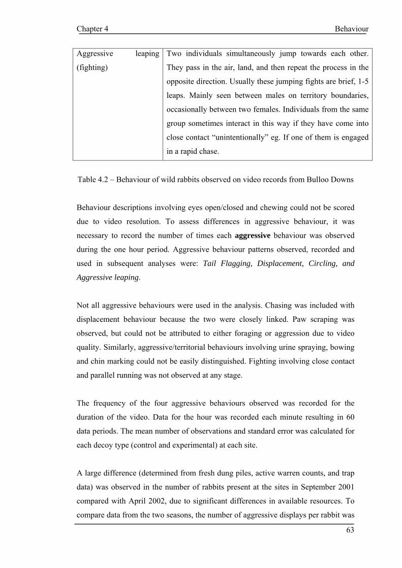
Chapter 4 Behaviour
Aggressive leaping
(fighting)
Two individuals simultaneously jump towards each other.
They pass in the air, land, and then repeat the process in the
opposite direction. Usually these jumping fights are brief, 1-5
leaps. Mainly seen between males on territory boundaries,
occasionally between two females. Individuals from the same
group sometimes interact in this way if they have come into
close contact “unintentionally” eg. If one of them is engaged
in a rapid chase.
Table 4.2 – Behaviour of wild rabbits observed on video records from Bulloo Downs
Behaviour descriptions involving eyes open/closed and chewing could not be scored
due to video resolution. To assess differences in aggressive behaviour, it was
necessary to record the number of times each aggressive behaviour was observed
during the one hour period. Aggressive behaviour patterns observed, recorded and
used in subsequent analyses were: Tail Flagging, Displacement, Circling, and
Aggressive leaping.
Not all aggressive behaviours were used in the analysis. Chasing was included with
displacement behaviour because the two were closely linked. Paw scraping was
observed, but could not be attributed to either foraging or aggression due to video
quality. Similarly, aggressive/territorial behaviours involving urine spraying, bowing
and chin marking could not be easily distinguished. Fighting involving close contact
and parallel running was not observed at any stage.
The frequency of the four aggressive behaviours observed was recorded for the
duration of the video. Data for the hour was recorded each minute resulting in 60
data periods. The mean number of observations and standard error was calculated for
each decoy type (control and experimental) at each site.
A large difference (determined from fresh dung piles, active warren counts, and trap
data) was observed in the number of rabbits present at the sites in September 2001
compared with April 2002, due to significant differences in available resources. To
compare data from the two seasons, the number of aggressive displays per rabbit was
63

Chapter 4 Behaviour
calculated for each video tape, then averaged for each decoy type per site and
standard errors calculated. The calculation was performed by dividing the count of
behaviour in each minute period by the number of rabbits observed within 2m of the
cage for the corresponding period.
Results
Habitat Conditions
Active warren numbers were lower at both sites in 2002 compared with 2001. The
smallest reduction occurred at site 3, where the 2002 count was 55% of the 2001
count; the largest difference occurred at site 2, where the 2002 count was only 18%
of the 2001 count (table 4.3).
YEAR SITE ACTIVE INACTIVE
2001 1 61 9
2001 2 33 3
2001 3 138 12
2002 1 26 59
2002 2 6 1
2002 3 76 54
Table 4.3 – Active and Inactive Warren Count Data for 2001 and 2002
During each field trip, a total of 840 trap nights were used. In September 2001, a
total of 375 rabbits were trapped; 126 were male, 159 were female, and 90 were too
young to determine sex. Of the 375 individuals captured, 188 were recaptures. The
average weight of males captured was 892.5g (std error = 44.8g), the average weight
of females captured was 1135.7g (std error = 44.3g), and the average weight of
kittens captured that were able to be weighed was 340g (n=7; std error = 25.9g). A
scatterplot of rabbit weight v sex is shown in figure 4.2.
64

Chapter 4 Behaviour
2001 Capture Data Weight v Sex
g
500g
1000g
1500g
2000g
2500g
Sex
Wei
ght (
g)
Kitten Female Male
Figure 4.2 – 2001 Rabbit Weight v Sex (total captures). Favourable habitat
conditions prior to the trip induced a breeding cycle causing the variation in capture
weights.
In April 2002, a total of 169 rabbits were trapped; 99 were male, and 70 were female;
no kittens were trapped. The total number of 169 included 97 recaptures. The
average weight of male captures was 1527.8g (std error = 19.1g), and the average
weight of female captures was 1466.4g (std error = 23.7g). A scatterplot of rabbit
weight v sex is shown in figure 4.3. The effect of relatively poorer environmental
conditions in 2002 is evident in this data as fewer rabbits were trapped, no kittens
were trapped, and there was less variation in the weight of those rabbits that were
trapped.
65

Chapter 4 Behaviour
2002 Capture DataWeight v Sex
g
500g
1000g
1500g
2000g
2500g
Sex
Wei
ght (
g)
Male Female
Figure 4.3 – 2002 Rabbit Weight v Sex (total captures). Poor habitat conditions are
reflected in capture data where no kittens were observed and variation in weight was
reduced.
The average weight of rabbits retained as decoys was calculated for each
site/treatment/year and graphed with standard error (figure 4.4), where n denotes the
number of rabbits used as decoys at each site, and therefore denotes the number of
behaviour videos (samples) recorded at each site. Size of the decoys used in 2002
was significantly larger than 2001 due to lower resource availability (ie. tending
towards drought). Only the smallest, most immature males (no scrotal testes) were
retained as decoys during 2002.
66

Chapter 4 Behaviour
Mean Decoy Weight
0200400600800
10001200140016001800
1 2 3
Site
Wei
ght (
g) Control 2001Experimental 2001Control 2002Experimental 2002
n=1 n=8n=3 n=8 n=6 n=5 n=6 n=5 n=6 n=5 n=9
Figure 4.4 – Decoys used in 2002 were significantly larger than those used in 2001.
The mean percentage cover for each category (green, dry, absent) at each site on
each substrate during each year are presented in Table 4.4
Year Site Substrate Mean Percentage Cover std error
Absent Dry Green Absent Dry Green
Sep-01 1 Clay 34.0 50.3 15.7 8.4 4.7 4.0
Sep-01 1 Sand 27.3 13.7 59.0 4.6 4.8 3.8
Sep-01 2 Clay 60.3 22.6 17.1 14.6 9.2 5.5
Sep-01 2 Sand 39.5 5.6 54.9 4.3 0.9 4.0
Sep-01 3 Clay 76.5 13.5 10.0 4.7 3.1 3.1
Sep-01 3 Sand 46.4 14.9 38.7 4.3 6.3 4.3
Apr-02 1 Clay 91.7 8.3 0.0 2.0 2.0 0.0
Apr-02 1 Sand 79.7 15.3 5.0 3.4 2.1 1.7
Apr-02 2 Clay 80.0 19.0 1.0 3.3 3.5 0.6
Apr-02 2 Sand 80.3 15.7 4.0 3.0 2.4 1.1
Apr-02 3 Clay 89.0 10.1 0.9 2.0 1.6 0.4
Apr-02 3 Sand 56.2 42.5 1.3 10.0 9.4 0.6
Table 4.4 – Mean percentage cover across all sites/substrates/years.
67

Chapter 4 Behaviour
A comparison of percentage vegetation cover between years shows a large decrease
in the amount of available green vegetation in 2002 across all sites. While
environmental conditions were in general much worse in 2002 due to drought, micro-
differences were also apparent among sites within the season with respect to the total
amount of vegetation available (both green and dry). Vegetation data are better
displayed using the following graphs of mean percentage cover and 95% confidence
interval at each site (Fig 4.5 to 4.7).
Figure 4.5 – Mean percent cover (+/- 95%CI) of the different vegetation types on
sand and clay at Site 1 for September 2001 and April 2002
68

Chapter 4 Behaviour
Figure 4.6 – Mean percent cover (+/- 95%CI) of the different vegetation types on
sand and clay at Site 2 for September 2001 and April 2002
69
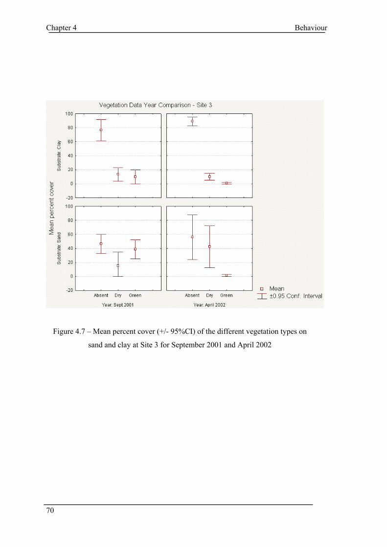
Chapter 4 Behaviour
Figure 4.7 – Mean percent cover (+/- 95%CI) of the different vegetation types on
sand and clay at Site 3 for September 2001 and April 2002
70

Chapter 4 Behaviour
Resource / Individual Index
The calculation of the resource/individual index (R/I) was based on the average
amount of green vegetation on sand substrates across the three sites; and the total
number of unique rabbit captures (ie. ignoring recaptures) collected during each
sampling trip. The index facilitates comparison between seasons when there were
observed differences in the distribution of food and the size of rabbit populations.
There was a much greater abundance of food in September (R/I = 0.27) relative to
April (R/I = 0.05).
Behaviour
A scatterplot of the rabbits observed vs total behaviour count (Fig 4.8) shows a clear
correlation in the raw data between these variables. It is for this reason, that all
subsequent analyses were performed on a transformed data set (behaviour per
rabbit), which removed any potential density effects interfering with analysis of
behaviour.
71

Chapter 4 Behaviour
Scatterplot - Both years data - All Behaviours (summed) vs Rabbit NumbersTotal Behaviours = -9.4059+3.8336*x
-10 0 10 20 30 40 50 60 70 80 90
Number of Rabbits
-50
0
50
100
150
200
250
300
350
400
Tota
l Beh
avio
ur C
ount
Rabbit Number:Total Behaviours: r 2 = 0.7951; r = 0.8917, p = 00.0000
Figure 4.8 – The amount of behaviour observed is correlated to the number of rabbits
present.
Totals of aggressive behaviour per rabbit were calculated for the one hour test
period. Values were tested using ANOVA within each year and treatment
combination to determine if data from all sites could be pooled for further analysis.
During September 2001, the mean summed control data at each site were not
significantly different among sites, F(2, 9) = 1.38, p = 0.30; and the mean summed
experimental data were not significantly different among sites, F(2, 16) = 0.98, p =
0.40.
During April 2002, the mean summed control data at sites 1 and 3 (site 2 was
excluded due to problems with dingos) were not significantly different t = -1.28
d.f.=6 p = 0.25; and the mean summed experimental data were significantly different
among sites 1 and 3, t = -2.43 d.f. = 15, p = 0.03. The differences in experimental
72

Chapter 4 Behaviour
data in April 2002 are probably due to the micro-differences in the resource levels at
each site, and therefore the data could not be pooled for further analysis. A plot of the
mean of each site and treatment with 95% confidence intervals follows (figure 4.9).
Figure 4.9 – Mean Plot of Sum Aggressive Behaviour per Rabbit per Hour for each
year shows no clear differences between treatments or years because of large error
margins
A students t-test was used to test for significant differences between the mean values
of control (pooled) and experimental (pooled) data in September 2001; and the
separate site means of control and experimental data in April 2002. There were no
significant differences observed in any instance. T tests were also used to test for
differences in control (pooled) data between years and experimental data (at each
site) between years. No significant differences were observed.
73
Chapter 4 Behaviour
74
Data were averaged for each year, site, and treatment combination. The graphs of
total aggressive behaviour per rabbit for each minute of observation (1hour total) are
presented in Figures 4.10 – 4.20 on the following pages; and show the distribution of
aggressive behaviour (per rabbit) throughout the data collection period (1hr).

75
18/09/01 Site1 t4 Control Total Behaviours per rabbit(total individuals = 11; total behav/rabbit = 19)
0
0.5
1
1.5
2
2.5
3
1 4 7 10 13 16 19 22 25 28 31 34 37 40 43 46 49 52 55 58
Time (min)
Beh
avio
urs
BehavioursMean behav/min observation
Figure 4.10 – Aggressive behaviour per rabbit at Site 1 for control rabbits in September 2001 (n=1)
75

76
Sept 2001 Site1 Expt Avg Total Behaviours per Rabbit(avg tot ind. = 12.88; avg tot behav/rabbit = 20.44)
0
0.5
1
1.5
2
2.5
3
1 4 7 10 13 16 19 22 25 28 31 34 37 40 43 46 49 52 55 58
Time (min)
avg
beha
viou
rs/ra
bbit
Avg behavioursmean behav/min observation
Figure 4.11 – Aggressive behaviour per rabbit at Site 1 for experimental rabbits in September 2001 (n=8)
76

77
Sept 2001 Site2 Control Avg Total Behaviours per rabbit(avg total ind. = 24; avg tot behav/rabbit = 28.16)
0
0.5
1
1.5
2
2.5
3
1 4 7 10 13 16 19 22 25 28 31 34 37 40 43 46 49 52 55 58
Time (min)
Avg
beh
avio
urs/
rabb
it
Avg behavioursMean behav/min observation
Figure 4.12 – Aggressive behaviour per rabbit at Site 2 for control rabbits in September 2001 (n=6)
77

78
Sept 2001 Site2 Expt Avg Total Behaviours per Rabbit(avg total ind. = 18.6; avg tot behav/rabbit = 27.19)
0
0.5
1
1.5
2
2.5
3
1 4 7 10 13 16 19 22 25 28 31 34 37 40 43 46 49 52 55 58
Time (min)
Avg
beh
avio
urs/
Rab
bit
Avg behavioursMean behav/min observation
Figure 4.13 – Aggressive behaviour per rabbit at Site 2 for experimental rabbits in September 2001 (n=5)
78

79
Sept 2001 Site3 Control Avg Total Behaviour per Rabbit(avg tot rabbits = 28.8; avg tot behav/rabbit = 40.91)
0
0.5
1
1.5
2
2.5
3
1 4 7 10 13 16 19 22 25 28 31 34 37 40 43 46 49 52 55 58
Time (min)
Avg
Beh
avio
ur/R
abbi
t
Avg behaviourMean behav/min observation
Figure 4.14 – Aggressive behaviour per rabbit at Site 3 for control rabbits in September 2001 (n=5)
79

80
Sept 2001 Site 3 Expt Avg Total Behaviour per Rabbit(avg total rabbits = 32.8; Avg Tot Behav/Rabbit = 33.6)
0
0.5
1
1.5
2
2.5
3
1 4 7 10 13 16 19 22 25 28 31 34 37 40 43 46 49 52 55 58
Time (min)
Avg
Beh
avio
ur/R
abbi
t
Avg BehaviourMean behav/min observation
Figure 4.15 – Aggressive behaviour per rabbit at Site 3 for experimental rabbits in September 2001 (n=6)
80

81
April 2002 Site 1 Control Avg Total Behaviours per rabbit(avg tot ind. = 10.66; avg tot behav/rabbit = 13.78)
0
0.5
1
1.5
2
2.5
3
1 4 7 10 13 16 19 22 25 28 31 34 37 40 43 46 49 52 55 58
Time (min)
avg
beha
viou
rs/ra
bbit
avg behavioursmean behav/min observation
Figure 4.16 – Aggressive behaviour per rabbit at Site 1 for control rabbits in April 2002 (n=3)
81
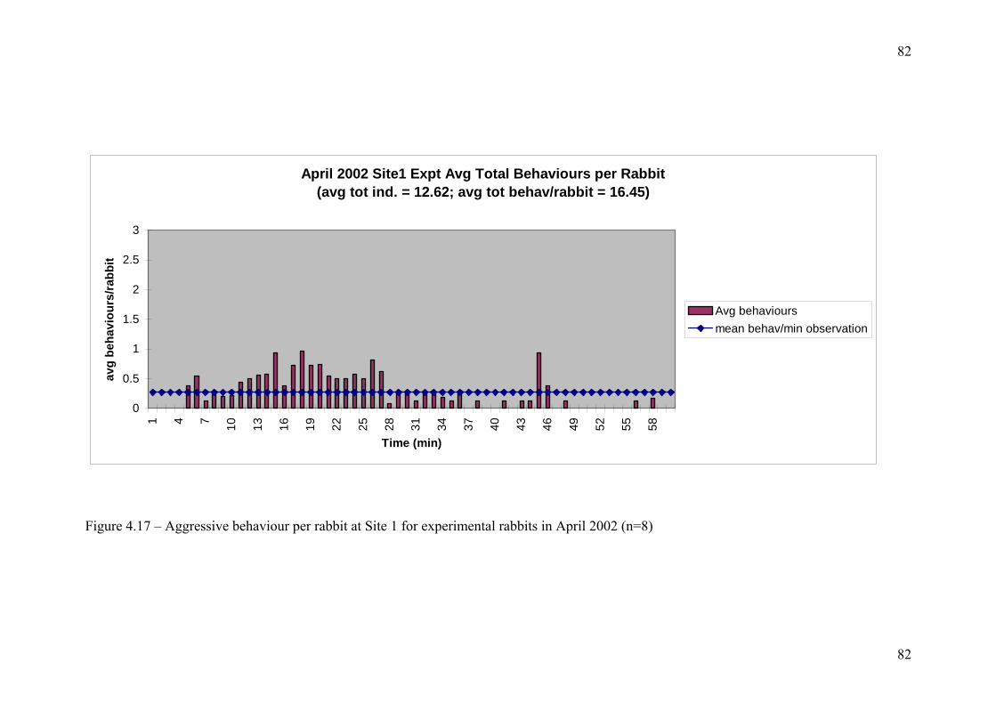
82
April 2002 Site1 Expt Avg Total Behaviours per Rabbit(avg tot ind. = 12.62; avg tot behav/rabbit = 16.45)
0
0.5
1
1.5
2
2.5
3
1 4 7 10 13 16 19 22 25 28 31 34 37 40 43 46 49 52 55 58
Time (min)
avg
beha
viou
rs/ra
bbit
Avg behavioursmean behav/min observation
Figure 4.17 – Aggressive behaviour per rabbit at Site 1 for experimental rabbits in April 2002 (n=8)
82

83
April 2002 Site2 Expt Avg Total Behaviours per Rabbit(avg tot ind. = 3.6; avg tot behav/rabbit = 5.5)
0
0.5
1
1.5
2
2.5
3
1 4 7 10 13 16 19 22 25 28 31 34 37 40 43 46 49 52 55 58
Time (min)
avg
beha
viou
rs/ra
bbit
avg behavioursmean behav/min observation
Figure 4.18 – Aggressive behaviour per rabbit at Site 2 for experimental rabbits in April 2002 (n=6). This site was severely affected by dingo activity.
83

84
April 2002 Site3 Control Avg Total Behaviours per Rabbit(avg tot ind. = 29.8; avg tot behav/rabbit = 35.35)
0
0.5
1
1.5
2
2.5
3
1 4 7 10 13 16 19 22 25 28 31 34 37 40 43 46 49 52 55 58
Time (min)
Avg
beh
avio
urs/
rabb
it
avg behavioursmean behav/min observation
Figure 4.19 – Aggressive behaviour per rabbit at Site 3 for control rabbits in April 2002 (n=5)
84

85
85
April 2002 Site3 Expt Avg Total Behaviours per Rabbit(avg tot ind. = 17.4; avg tot behav/rabbit = 29.93)
0
0.5
1
1.5
2
2.5
3
1 4 7 10 13 16 19 22 25 28 31 34 37 40 43 46 49 52 55 58
time (min)
avg
beha
viou
rs/ra
bbit
avg behaviourmean behav/min observation
Figure 4.20 – Aggressive behaviour per rabbit at Site 3 for experimental rabbits in April 2002 (n=9)

Chapter 4 Behaviour
86
The data for each hour was grouped into 6 intervals of 10 minutes duration, this was
done to remove most of the “zero” scores, while still obtaining an overview of any
trends during the filming period. It also allowed the following comparisons (of each
data period) via statistical methods:
Within year, site, and treatment
Within year and site, between treatments
Within year, between sites, within treatments
Between years, within site and treatments
Within year, site, and treatment (ANOVA).
During September 2001, at Site 1 and Site 2, both control and experimental
treatments were not significantly different for any time period.
Site 1 expt F(5, 42) = 1.07, p = 0.39; Site 2 cont F(5, 30) = 0.63, p = 0.68; Site 2 expt
F(5, 24) = 2.52, p = 0.06. Site 3 control data shows a significant difference, F(5, 24)
= 3.18, p = 0.02, the significant result occurs due to the first time period (0-10min)
having significantly more aggressive behaviour per rabbit than the last two time
periods (40-60min) as shown in the decreasing trend (figure 4.23). Site 3
experimental data shows that the first time period (0-10min) was significantly
different from the rest of the hour (10-60min) F (5, 30) = 7.17, p = 0.0002. This is
confirmed by the graph in figure 4.23 that shows the significantly higher mean.

Chapter 4 Behaviour
87
Figure 4.21 – September 2001 Site 1 Aggressive Behaviour per Rabbit in 10min
intervals is not significantly different due to large error margins

Chapter 4 Behaviour
88
Figure 4.22 – September 2001 Site 2 Aggressive Behaviour per Rabbit in 10min
intervals is not significantly different due to large error margins

Chapter 4 Behaviour
89
Figure 4.23 – September 2001 Site 3 Aggressive Behaviour per Rabbit is
significantly higher in the 0-10min phase
During April 2002, there were no significant differences in the control data for any
site (1 & 3 – note that no control data was collected at site 2, and the experimental
data at site 2 was severely affected by dingo activity.). Site 1 cont F(5, 12) = 1.03, p
= 0.45; Site 3 cont F(5, 24) = 2.31, p = 0.08. The experimental data at site 1 and 3
was significantly different within each hour. Site 1 experimental F(5, 42) = 4.21, p =
0.003 was significant due to the 10-20min period being significantly higher than all
other periods except the 20-30min. Site 3 experimental F(5, 48) = 3.60, p = 0.008
was significant due to the 0-10min period being significantly higher than the period
from 20-60min, the 10-20min period was part of the decreasing trend from the initial
period to the lower levels observed in the remainder of the hour. Figures 4.24 – 4.26
show the graphs mean values.

Chapter 4 Behaviour
90
Figure 4.24 – April 2002 Site 1 Aggressive Behaviour per Rabbit is significantly
higher in 10-20min period for experimental data

Chapter 4 Behaviour
91
Figure 4.25 – April 2002 Site 2 Aggressive Behaviour per Rabbit was severely
affected by the activity of dingos

Chapter 4 Behaviour
92
Figure 4.26 – April 2002 Site 3 Aggressive Behaviour per Rabbit is significantly
higher in 0-10min period for experimental data

Chapter 4 Behaviour
93
Within year and site, between treatments (t-test)
T tests were used to compare the mean number of aggressive behaviours per rabbit
during each time period. Results for each site are tabulated below (tables 4.5 – 4.9)
and significant results are highlighted. Across all tests, the only significant difference
between control and experimental data was observed in the 30-40min period at site 2
during September 2001; a result most likely caused by the average experimental
value being very close to zero.
Mean
Expt
Mean
Cont
t-value df p Valid N
expt
Valid N
Cont
Std.Dev.
Expt
Std.Dev.
Cont
F-ratio
variances
p variances
0-10 1.8 0.0 0.6 7 0.60 8 1 2.8 0.0 0.0 1.0
10-20 4.6 4.0 0.1 7 0.93 8 1 6.1 0.0 0.0 1.0
20-30 6.3 4.0 0.3 7 0.76 8 1 6.9 0.0 0.0 1.0
30-40 3.9 5.0 -0.2 7 0.83 8 1 4.9 0.0 0.0 1.0
40-50 2.0 6.0 -1.3 7 0.24 8 1 2.9 0.0 0.0 1.0
50-60 1.9 0.0 0.4 7 0.72 8 1 4.8 0.0 0.0 1.0
Table 4.5 - September 2001 Site 1 Control v Experimental
Mean
Expt
Mean
Cont
t-value df p Valid N
expt
Valid N
Cont
Std.Dev.
Expt
Std.Dev.
Cont
F-ratio
variances
p variances
0-10 4.3 4.8 -0.2 9 0.87 5 6 4.0 5.3 1.7 0.6
10-20 8.7 4.8 1.4 9 0.21 5 6 5.4 4.1 1.8 0.5
20-30 6.8 4.7 0.7 9 0.48 5 6 4.1 5.0 1.5 0.7
30-40 0.9 7.1 -2.8 9 0.02 5 6 1.3 4.8 12.6 0.0
40-50 3.0 3.4 -0.2 9 0.87 5 6 4.8 2.2 4.6 0.1
50-60 3.5 3.3 0.1 9 0.94 5 6 2.3 3.3 2.2 0.5
Table 4.6 - September 2001 Site 2 Control v Experimental is significant during 30-
40min period

Chapter 4 Behaviour
94
Mean
Expt
Mean
Cont
t-value df p Valid N
expt
Valid N
Cont
Std.Dev.
Expt
Std.Dev.
Cont
F-ratio
variances
p variances
0-10 15.2 12.6 0.8 9 0.43 6 5 3.5 6.9 3.8 0.2
10-20 4.8 8.8 -1.2 9 0.27 6 5 5.4 5.8 1.2 0.9
20-30 5.2 6.2 -0.3 9 0.79 6 5 6.4 5.9 1.2 0.9
30-40 3.4 8.6 -2.0 9 0.07 6 5 2.9 5.6 3.8 0.2
40-50 3.3 3.2 0.0 9 0.97 6 5 4.7 2.5 3.6 0.2
50-60 1.7 1.6 0.1 9 0.92 6 5 2.6 0.7 14.3 0.0
Table 4.7 - September 2001 Site 3 Control v Experimental
Mean
Expt
Mean
Cont
t-value df p Valid N
expt
Valid N
Cont
Std.Dev.
Expt
Std.Dev.
Cont
F-ratio
variances
p variances
0-10 1.8 2.3 -0.2 9 0.85 8 3 4.6 4.0 1.3 1.0
10-20 6.6 3.2 1.2 9 0.27 8 3 3.8 5.6 2.2 0.4
20-30 4.7 5.4 -0.3 9 0.79 8 3 4.3 0.8 29.5 0.1
30-40 1.4 1.0 0.2 9 0.81 8 3 2.2 1.7 1.7 0.9
40-50 1.8 1.5 0.2 9 0.85 8 3 2.4 2.6 1.2 0.7
50-60 0.3 0.3 -0.1 9 0.91 8 3 0.5 0.6 1.1 0.8
Table 4.8 - April 2002 Site 1 Control v Experimental
Mean
Expt
Mean
Cont
t-value df p Valid N
expt
Valid N
Cont
Std.Dev.
Expt
Std.Dev.
Cont
F-ratio
variances
p variances
0-10 10.5 11.5 -0.3 12 0.76 9 5 6.1 2.9 4.5 0.2
10-20 6.4 8.5 -0.5 12 0.62 9 5 6.08 9.4 2.4 0.3
20-30 3.2 8.3 -1.8 12 0.10 9 5 3.31 7.5 5.2 0.0
30-40 4.1 2.3 0.7 12 0.51 9 5 5.38 3.2 2.9 0.3
40-50 3.8 1.1 1.2 12 0.27 9 5 4.82 2.4 4.1 0.2
50-60 1.9 3.7 -0.7 12 0.50 9 5 2.28 7.2 10.0 0.0
Table 4.9 - April 2002 Site 3 Control v Experimental

Chapter 4 Behaviour
95
Within year, between sites, within treatments (ANOVA)
Variation between sites in aggressive behaviour per rabbit within season and
treatment was measured using one way ANOVA. An analysis was performed for
each time period. There were no significant differences in control data among sites
during September 2001 (table 4.10).
Time Period (min) Statistic
0-10 F(2, 9) = 3.1, p = 0.09
10-20 F(2, 9) = 1.0, p = 0.40
20-30 F(2, 9) = 0.1, p = 0.88
30-40 F(2, 9) = 0.3, p = 0.78
40-50 F(2, 9) = 0.6, p = 0.56
50-60 F(2, 9) = 1.1, p = 0.37
Table 4.10 - September 2001 Control data shows no difference among sites
A significant difference, however, was observed in experimental data among sites
during September 2001 only for the 0-10min period (table 4.11). This resulted from
the relative level of aggression per rabbit at site 3 being much greater than at sites 1
and 2. For all other periods there were no significant differences among sites. This
result highlights the behavioural variation in the one hour period between sites
during the same season, which may be caused by the micro-variation in resource
levels at each site during the season, however further research is required to prove
this conclusively.

Chapter 4 Behaviour
96
Time Period (min) Statistic
0-10 F(2, 16) = 28.9, p = 0.00
10-20 F(2, 16) = 0.9, p = 0.43
20-30 F(2, 16) = 0.1, p = 0.90
30-40 F(2, 16) = 1.1, p = 0.37
40-50 F(2, 16) = 0.2, p = 0.82
50-60 F(2, 16) = 0.4, p = 0.70
Table 4.11 - September 2001 Experimental data is significantly different for 0-10min
Site 2 was excluded from further analysis in April 2002 because of high activity of
dingos interfering with rabbit behaviour, therefore, t tests were used to compare data
only between sites 1 and 3. There was a significant difference in control data among
sites during April 2002 only for the 0-10min period. The result was caused by the
aggression per rabbit at site 3 being much greater than site 1. For all other periods
there were no significant differences among sites (table 4.12).
Mean
Site 1
Mean
Site 3
t-value df p Valid N
Site 1
Valid N
Site 3
Std.Dev.
Site 1
Std.Dev.
Site 3
F-ratio
variances
p variances
0-10 2.3 11.5 -3.8 6 0.01 3 5 4.0 2.9 1.9 0.5
10-20 3.2 8.5 -0.9 6 0.42 3 5 5.6 9.4 2.8 0.6
20-30 5.4 8.3 -0.7 6 0.54 3 5 0.8 7.5 90.7 0.0
30-40 1.0 2.3 -0.6 6 0.54 3 5 1.7 3.2 3.3 0.5
40-50 1.5 1.1 0.2 6 0.82 3 5 2.6 2.4 1.2 0.8
50-60 0.3 3.7 -0.8 6 0.46 3 5 0.6 7.2 155.9 0.0
Table 4.12 - April 2002 Control Data - Site 3 is significantly higher during 0-10min
than Site 1

Chapter 4 Behaviour
97
There was a significant difference in experimental data among sites during April
2002 only for the 0-10min period. The result was caused by the level of aggression
per rabbit at site 3 being much greater than site 1. For all other periods no significant
differences were observed among sites (table 4.13).
Mean
Site 1
Mean
Site 3
t-value df p Valid N
Site 1
Valid N
Site 3
Std.Dev.
Site 1
Std.Dev.
Site 3
F-ratio
variances
p variances
0-10 1.8 10.5 -3.3 15 0.01 8 9 4.6 6.1 1.8 0.4
10-20 6.6 6.4 0.1 15 0.95 8 9 3.8 6.1 2.6 0.2
20-30 4.7 3.2 0.8 15 0.45 8 9 4.3 3.3 1.7 0.5
30-40 1.4 4.1 -1.3 15 0.20 8 9 2.2 5.4 5.8 0.0
40-50 1.8 3.8 -1.0 15 0.32 8 9 2.4 4.8 4.1 0.1
50-60 0.3 1.9 -2.0 15 0.07 8 9 0.5 2.3 17.3 0.0
Table 4.13 - April 2002 Experimental Data - Site 3 is significantly higher during 0-
10min than Site 1
Between years, within site and treatments (t test)
The differences observed among sites prevented the pooling of all site data to test
between years, however, as there were no significant differences between control and
experimental treatments at each site – the data were combined (to give a larger data
set) for each site to allow a comparison of the aggressive behaviour per rabbit
between years for sites 1 and 3 (tables 4.14 – 4.15).

Chapter 4 Behaviour
98
Mean
Sept
Mean
April
t-value df p Valid N
Sept
Valid N
April
Std.Dev.
Sept
Std.Dev.
April
F-ratio
variances
p variances
0-10 1.6 1.9 -0.2 18 0.87 9 11 2.7 4.2 2.5 0.2
10-20 4.5 5.7 -0.5 18 0.62 9 11 5.8 4.3 1.8 0.4
20-30 6.0 4.9 0.5 18 0.62 9 11 6.5 3.6 3.2 0.1
30-40 4.0 1.3 1.8 18 0.09 9 11 4.6 2.0 5.1 0.0
40-50 2.4 1.7 0.6 18 0.57 9 11 3.1 2.3 1.8 0.4
50-60 1.7 0.3 1.0 18 0.32 9 11 4.6 0.5 75.6 0.0
Table 4.14 - Site 1 – September 2001 v April 2002 – no difference
Mean
Sept
Mean
April
t-value df p Valid N
Sept
Valid N
April
Std.Dev.
Sept
Std.Dev.
April
F-ratio
variances
p variances
0-10 14.0 10.9 1.5 23 0.14 11 14 5.2 5.1 1.0 0.9
10-20 6.6 7.1 -0.2 23 0.85 11 14 5.7 7.1 1.6 0.5
20-30 5.6 5.1 0.2 23 0.81 11 14 5.8 5.5 1.1 0.8
30-40 5.8 3.4 1.2 23 0.24 11 14 4.9 4.7 1.1 0.8
40-50 3.2 2.8 0.3 23 0.79 11 14 3.7 4.2 1.3 0.7
50-60 1.6 2.6 -0.6 23 0.53 11 14 1.9 4.5 5.5 0.0
Table 4.15 - Site 3 – September 2001 v April 2002 – no difference
No significant differences were observed between years in any time period, at any
site, though the data does show that site 1 consistently had a latency period for the
first 10 minutes, while site 3 had the highest levels of activity in the initial period.
A general linear model (Statistica) was used to investigate the general trends within
the data set. The process is an extension of the multiple regression / multivariate
regression models that allows for linear combinations or transformations of multiple
variables and also permits examination of repeated measure factors (StatSoft, 2006).
The model was applied across the entire data set to identify trends in the amount of
aggressive behaviour per rabbit with respect to the following variables: Year, Site,
Treatment, Time (within the hour). The process did not identify statistically

Chapter 4 Behaviour
99
significant effects of the previously mentioned variables. However, the ability to
examine and view all data on one graph did identify one trend that was not apparent
from other analyses. The graph of mean behaviour/rabbit at each site plotted against
Year, and Treatment (Figure 4.27) shows a consistent decrease in the amount of
rabbit behaviour at each site between years, for the treatment in question. Sites 1 and
3 (Site 2 is excluded due to high levels of dingo activity) exhibited greater amounts
of behaviour responses in 2001 compared with 2002. At each site, the degree of
reduced behaviour between years was virtually identical; and while the reduction was
less in the experimental data, the same pattern was observed in both the control and
experimental data sets. This result highlights a consistent effect of drier conditions in
2002 on the amount of aggressive behaviour per rabbit – that is, an overall reduction
in activity.
Figure 4.27 – General Linear Modelling identified a consistent reduction in
behaviour between years for each treatment at each site (Site 2 excluded due to dingo
activity).

Chapter 4 Behaviour
100
Sixty minutes of video data was collected each time based on power limitations of
the experiment. It enabled an examination to identify any behavioural trends that
may occur throughout the hour. However, previous studies of rabbit territorial
behaviour suggest that any aggressive response to a decoy (ie. intruder) is most likely
to occur quite soon after the decoy is introduced to the site (B.Cooke and D.Berman
pers comm). This response was most evident at Site 3. Therefore, data from only the
first 15 minutes of each tape were analysed and compared in further detail to
examine differences in aggressive response towards known (control) and unknown
(experimental) rabbits.
This analysis used a different time period (15 mins) than had been used previously.
A 10 minute time interval was used for overall analysis (ANOVA etc) of the entire
dataset; the grouping removed a lot of the “zeros” to facilitate statistical analysis,
whilst still enabling examination of trends during the hour as the data were split into
6 discrete periods. The 15min initial period was chosen for the analysis of the critical
period when the most aggressive activity occurs based on comments from field
experts (ie. if an aggressive territorial response were to occur in a natural system, it
would happen within 15mins of trespassing, or not at all). To split the entire data set
into 15min periods (for the previous analyses simply for the sake of consistent
numbers) would reduce the number of discrete time periods to 4 per hour and make it
harder to justify as an examination of trends over one hour. Hence two different time
periods were used in the two different analyses.
The average percentage aggressive behaviour (out of total aggressive behaviour per
rabbit observed) occurring in the first 15 minutes are presented below in table 4.16.
At all sites (where sufficient data exists), there was a higher percentage of aggressive
behaviour evident in the experimental treatments compared with control treatments
during the first 15 minutes of the test period.

Chapter 4 Behaviour
101
Year Site Treatment Percentage
Sept 2001 1 Control 10.5
Sept 2001 1 Experimental 21.9
Sept 2001 2 Control 27.9
Sept 2001 2 Experimental 35.4
Sept 2001 3 Control 38.9
Sept 2001 3 Experimental 53.8
April 2002 1 Control 20.6
April 2002 1 Experimental 29.0
April 2002 2 Experimental 14.9
April 2002 3 Control 45.3
April 2002 3 Experimental 52.3
Table 4.16 – Percentage of Total Aggressive Behaviour Occurring in first 15mins is
higher for experimental sites
The proportion of total aggressive behaviour in the experimental and control data at
15 minutes are presented in table 4.17 below. The values are calculated by dividing
the number of behaviours observed at 15 minutes (either experimental or control), by
the sum of the number of behaviours for each class, as defined by the following
formula:
Pexpt15 = Nexpt15 / (Nexpt15 + Ncont15) and Pcont15 = Ncont15 / (Nexpt15 + Ncont15)
Year Site Pexpt Pcont
September 1 0.70 0.30 September 2 0.59 0.41 September 3 0.63 0.37
April 1 0.76 0.24 April 3 0.46 0.54
Table 4.17 – Proportion of aggressive behaviour occurring in first 15 minutes

Chapter 4 Behaviour
102
If there was no difference in response to control or experimental rabbits, then the
proportion in each class in Table 4.17 should be 0.5. It is important to remember that
this is a test of the treatments only within the replicated design. The previously
identified effect of seasonal difference (however slight it may be), was not a factor
included in this analysis as the data were examined within season and site factors. A
two-tailed, one sample t-test with the test value = 0.5 was performed to test the
significance of the values. The difference between proportions for September was
significant (p = 0.05, df = 2), and the proportions of control to experimental
responses for April were not significantly different (p = 0.58, df = 1).

Chapter 4 Behaviour
103
Discussion
The purpose of the behaviour component of the study was to determine
quantitatively, if aggressive behaviour in the European rabbit varied under different
resource conditions. It therefore required tests to be conducted under different
environmental conditions. It was quite clear from personal observation that
environmental conditions were very different during the two sampling trips; and this
was confirmed by the analysis of warren counts, capture data, and vegetation
transects. A good reflection of the effect of the minor rainfall that occurred in June
2001 were the data relating to individual weights of rabbit captures (Figure 4.2).
Rainfall initiated a period of breeding, which is why weight of rabbits ranged from
200g to over 2000g. The break in the data lines in figure 4.2 indicates that the time
since rainfall was around 3 months because rabbits can be aged by weight up to
1000g at the rate of 10g per day (D.Berman pers comm). Weight of female rabbits
during September 2001 was more variable than male rabbits due to breeding cycle,
some may have been pregnant with late litters and others were in poor condition after
having produced their litters.
Rabbit capture data for April 2002 also demonstrate the change in resource quality
from September 2001. No kittens were captured in 2002, and the range in weight for
adult males and females was nearly identical. These differences are illustrated by the
graph of mean decoy weight (i.e. only those rabbits used in filming experiments were
considered) for both sampling trips (figure 4.4). An extensive search of literature
found no studies reporting the effect of decoy size on behavioural response, however,
given the large difference between mean decoy weights (between years) in this study,
the possibility that decoy size introduced an unwanted variable into the experiment
cannot be excluded.
One of the best ways to elicit a territorial response is through the use of a decoy, and
there are many examples of decoy use in the literature. Hau et al. (2004) used decoys
to conduct simulated territorial intrusions in populations of the spotted antbird
(Hylophylax n. naevioides) to examine hormonal control of territorial aggression.

Chapter 4 Behaviour
104
They found that antbirds can produce hormones (during the non-breeding season)
that may serve as a precursor of sex steroids for the regulation of year round
territorial behaviour (Hau et al. 2004). Wiklund and Village (1992) used caged
decoys to simulate territorial intrusion in the European Kestral (Falco tinnunculus),
and found that territorial behaviour varied depending on the stage of the breeding
cycle. The simulated territorial intrusion approach was a crucial aspect of the present
study.
Food availability is a key resource for wild rabbit populations, and quantification of
the differences in food availability between sampling trips was necessary in order to
test the hypothesis that wild rabbits may alter their social systems as a response to the
amount and distribution of favourable habitat. Transects were used to assess the
amount of green vegetation, representing edible food for rabbits. During September
2001, only sand substrates exhibited a moderate level of green cover, whereas clay
substrates had low amounts of green cover. This was a further indication of the poor
environmental conditions present and a reflection of the amount of rainfall from
June/July 2001 and the weather conditions during the intervening period. If a larger
amount of rainfall had occurred during the winter period, a higher level of green
cover would be expected on clay substrates as well as on sand substrates. The months
between September 2001 and April 2002 were very hot and no rainfall was recorded
at all, and the effect of this is clearly illustrated in the vegetation graphs. Extremely
low levels of green vegetation were present at all sites on all substrates (0-5%). As a
corollary, there were high levels of bare ground at all sites and substrates in April
2002, except at site 3 on the sand substrate, where there was a high level of dry
vegetation present (42%). This effect at site 3 may have been caused by the slightly
larger size of the sand hill and the presence of a few more established trees on the hill
that may have aided in local moisture retention.
The resource/individual index (RI) was five times larger in September 2001
compared with April 2002. It highlights a qualitative difference between the two
sample periods, ie. there was an actual difference in the availability of food to
individual rabbits, and not merely fewer individuals eating less food. The value of RI

Chapter 4 Behaviour
105
for April 2002 (0.05), is an additional indicator of the drought that affected the
region and the population systems within.
Statistical analysis of total rabbit aggressive behaviour data identified differences
solely in experimental data between sites 1 and 3 during April 2002. Aside from
preventing the pooling of data for further analysis, this result suggests that rabbit
behaviour differed at these sites. Differences may have been caused by the variance
of site 3 with respect to the amount of bare ground, dry and green vegetation;
however, if this was so, then a similar difference might also be expected in the
control data for those sites. The April 2002 control data of site 3 has a larger mean,
however, the variance around the mean is so large that a significant difference was
not evident.
A general trend was present (albeit masked by high variances) that suggests flexible
behaviour systems is an attribute of rabbit populations in arid environments. Table
4.16 shows that at every site during both years, where sufficient data exists, there
was a higher percentage of total aggressive response recorded during the first 15
minutes for all experimental data versus control data at all sites. The actual
percentages varied among sites, which most likely reflects the size of the
populations, the local environmental conditions, levels of resources present, and
relative activity levels of predators during the sampling trips. Table 4.17 shows the
proportion of control and experimental aggressive behaviour occurring in the first 15
minutes (in relation to the total amount of aggressive behaviour observed). As
discussed earlier, the initial time period appears critical in terms of territorial
defence; and it is evident that a difference in response occurred because the
proportions are not 0.5, which could be expected under identical response patterns.
The proportional difference in values was found to be statistically significant for
September 2001, however, it was non-significant in 2002 when environmental
conditions were most harsh. It is apparent, therefore, that under the most severe (ie.
drought) conditions it was not possible to detect a difference in aggressive response
to control and experimental rabbits.

Chapter 4 Behaviour
106
Control rabbits used in the experiments were ‘known’ to the test population and were
of low social rank. They therefore would likely generate less of an initial aggressive
response than will an experimental rabbit brought from outside the population.
Control rabbits, however, remained part of the social hierarchy within the territories
of capture, and therefore it is highly probable that any aggressive behaviour observed
against control rabbits were part of the normal social interactions among individuals
within a group. Evidence for this is provided by the lack of an initial burst of
aggressive behaviour as observed with experimental rabbits, and the general
accumulation of aggressive behaviour across the sampling hour. It is also unknown if
the released control rabbits were able to “learn” from their experience of being in the
cage, and what effect that might have on their response to a different rabbit being
presented at the same location on subsequent nights. Although fur marking prevented
re-use of the same individuals, there was evidence of recaptures at all sites (data not
presented) – particularly in 2002, when conditions were drier. It is possible that
recaptured rabbits became “trap happy” in order to utilise the food resource (chopped
carrot) within the traps. Recent example of other species exhibiting trap happy
behaviour can be found in Gibba turtles (Deforce et al. 2004), Australian fur seals
(Hume et al. 2002), and European badgers (Tuyttens et al. 1999).
Analysis of aggressive behaviour data was also conducted to assess differences in
behaviour over different time periods within the one hour sample in order to
investigate further the trend identified with analysis of sum total data.
During September 2001, within each site and treatment, the lack of significant
differences among time intervals at sites 1 and 2 indicates an even distribution of
aggressive behaviour across the sampling period. Site 3, however, exhibited a
decreasing trend that is consistent with the idea that most aggression occurs early
during the sampling time. A similar pattern was observed during April 2002 where
no significant difference was found among time intervals for the control data,
however, there were differences for the experimental data. During April at site 1,
there appeared to be a latency period of ten minutes before a burst of aggressive
activity followed by a gradual decline. At site 3 (April), the pattern matched

Chapter 4 Behaviour
107
September 2001 in that levels of aggression peaked in the first time interval and
gradually reduced. The observed trend of an early peak in aggressive behaviour
varied in strength among sites, which can be explained by the distribution of food
resources. Whilst the environmental conditions and food resources were different
between seasons, they were also not identical within a season. Therefore, variation in
behaviour patterns may be due to micro-variation in environmental and food
conditions among sites within each season. During September 2001, the collective
amount of vegetation (both dry and green) at each site on sand substrate was 73%,
61%, and 55% for sites 1-3 respectively, however, during April 2002 the vegetation
amount was reduced to approximately 20% at sites 1 and 2, and 44% at site 3. For
site 1, the large reduction in vegetation availability is a possible explanation for the
behaviour trend observed in April as opposed to the consistent level of behaviour
observed in September. For site 3, there was only minor change to the total amount
of vegetation available, which explains the similar patterns observed between
seasons at this site. It is probable that site 1 was in a much greater state of decline (in
a metapopulation sense) than site 3, due to a combination of the amount of vegetation
available and the general environmental conditions (ie the weather) – thus causing
the variation in the observed behavioural response between sites.
Effect of habitat variation on behaviour (in general) is extremely well studied,
however, as Brashares and Arcese (2002) comment, there are few species that vary
sufficiently in social behaviour to permit detailed intraspecific comparisons. (ie.
variable behaviour across different habitats). The vegetation component of this study
measured the variables of food quantity and quality; and counts of active warrens can
be used as an indicator of density – three habitat variables previously shown to
influence territoriality (Maher and Lott, 2000). Lombardi et al. (2003) examined the
ecological responses of the European rabbit to varied (3 types) habitats; scrubland
(dense cover, low food), grassland (little cover, high food), and ecotone between the
two. In the scrubland, rabbits were dispersed among cover, and in grassland, rabbits
were linked to aggregated burrows. Rabbits reached the highest abundance in
ecotone, whereas low food and refuge availability limited abundance in scrubland
and grassland respectively (Lombardi et al. 2003). Therefore, the study also showed

Chapter 4 Behaviour
108
that rabbits were able to modify behaviour patterns in order to adapt to specific
habitat conditions across a very small geographic area (2km separated all sites). The
significance of this is that while Lombardi et al. (2003) did not examine the genetic
structure of the rabbit populations, they would almost certainly have shared common
genes without significant structuring based on distances rabbits are known to
disperse (Williams et al. 1995). Taken together, this suggests that the rabbit
populations studied by Lombardi et al. (2003) were probably of the same genetic
stock, yet able to modify behaviour patterns across a small area.
There are several points of statistical relevance that require further comment:
1. Throughout the present study of rabbits in arid and semi-arid Australia,
statistically significant differences were not observed between control and
experimental (total) data due to the large variances present in the behavioural
data; and a posteriori one can infer that unless the trend had been extremely
strong, it would be highly unlikely to detect any underlying differences that
were present.
2. The use of correlation data does not necessarily imply cause and effect. Figure
4.8 illustrated a correlation between the total number of rabbits observed and
the total amount of behaviour, which was cause to use the calculation of
behaviour/rabbit to remove density effects between years. That is not to say
there is a cause and effect relationship between these variables; more likely,
the external factors influencing the number rabbits can be considered causal
for the effect of behaviour variability. This ideawill be explored further in
Chapter 5.
3. A type 1 error occurs when one statistically rejects a null hypothesis (based on
whatever level of α is set, usually 0.05) when it is fact true. It represents the
“false positive” scenario, which is particularly undesirable as it can result in
wasted efforts of further research that is unable to replicate the original
results (Statsoft, 2006). A type 2 error occurs when one fails to reject the null
hypothesis when the alternative is true; it effectively rejects the researcher’s
theory when it is actually correct. It is an unfortunate result when one
considers that valuable theories and technologies could be lost due to this

Chapter 4 Behaviour
109
type of error (Statsoft, 2006). When one encounters datasets like that
presented here (results affected by drought and disease) with a large amount
of statistically non-significant results – the question arises as to whether there
may be type 1 or 2 errors. Clearly, one cannot say without further research if
an error was committed. Based on the current data however, it would appear
that a type 2 error would more likely be committed in this instance. That is
not to say that a rigorous statistical approach has not been adhered to – where
the statistical results suggested the rejection of an hypothesis was necessary,
it was done. The only way to discount the effect of type 2 (and type 1) errors
on the results here (and the theory behind it regarding flexible behaviour) is
to replicate the experiments in times of greater resource abundance, thus
removing the potential impact of drought and disease from the data.
These data illustrate the differences between sites in terms of the size of local
populations and the manner in which each population behaved – the differences are
ultimately a reflection of the difficult environmental conditions that prevailed during
the study period. The fact that constant levels of aggression per rabbit were observed
across the hour test period in some instances does not suggest that rabbit aggression
will occur in this manner in non experimental situations. Additionally, the restraint of
the decoy rabbit within the study area precluded certain aggressive behaviour
patterns directed at the decoy from being observed and measured. Aggressive
fighting, chasing and displacement of territorial transgressors may occur very quickly
within the population systems used in this study under non-experimental conditions.
Site 3 was the only site during both September 2001 and April 2002 that had a
population of rabbits behaving with the largest number of aggressive responses in the
initial time interval. This is most likely due to the larger population size at site 3 as
indicated by warren count and personal observation. After initial aggressive displays
towards the decoy, which was restrained in a cage and hence could not escape the
site, resident rabbits may have been more concerned with social and or territorial
interactions within the population. This behavioural response is similar to that which
might be expected under non experimental conditions when a foreign rabbit enters a

Chapter 4 Behaviour
110
territory and is subsequently forced to leave after a short amount of time. Territorial
displacement is a strong behavioural indicator and (although manifest in different
ways) is observed in a variety of species such as American redstart (Marra, 2000),
woolly monkeys (White et al. 2000), common loons (Piper et al. 2000), trout
(Landergren, 1999), and gecko lizards (Petren, 1998).
While the cages used for trapping and restraining decoys were in place for a week
prior to video taping to avoid the neophobic effects described by Sunnucks (1998);
their presence in a natural system cannot be completely ignored in terms of their
effect upon the observed behaviour. It is assessed that sufficient attenuation was
achieved to minimize the effect on this study; however, one may consider it an
unavoidable facet of experimental field research.
Despite drought conditions, predators, and other associated problems, the results of
the behavioural component of this project support the potential for flexible social
patterns and variable territorial response in the European rabbit, which can be at least
in part explained by variability in resource availability. The potential was evident in
the variation in levels of aggressive behaviour response during the initial contact
period depending on the origin of the transgressor rabbit. The implications of the
potential for flexible social structures on general rabbit population dynamics and
their influence on population genetic structures are developed in the following
chapter.

Chapter 5 Discussion and Conclusions General Discussion
The ability to exhibit variable behaviour patterns is one mechanism that allows
animals to adapt to extant conditions. It is something that occurs across virtually all
animal species, with perhaps one of the most striking examples being carrion crows
in Japan that developed a behaviour pattern to use vehicles stopped at traffic lights to
crack walnuts (Nihei, 1995). For the European rabbit, however, survival in the arid
environments of western Queensland compared with that in more temperate climates
is very difficult without certain adaptations to lifestyle. This fact will hold true for
most species found in arid and non-arid climes. The adaptations required may take
several forms, and include patterns of feeding, methods for obtaining shelter, and
reproductive cycles; one or all of which may contribute to the formation of
metapopulations in arid environments (Hanski and Gilpin, 1991; Kutt, 2003).
The metapopulation dynamics of European rabbit populations in western Queensland
are in keeping with source-sink models as outlined earlier and supported by personal
observations and discussions with landholders. In dry times, the only rabbits that
survive live in proximity to permanent sources of water – the largest being the
Bulloo Lakes in the south-west of the Bulloo Downs property. When floodwaters
arrive to regenerate green pastures, they trigger a burst in reproduction that
subsequently initiates widespread dispersal to ‘sink’ type habitats.
Population Genetics
The cyclical nature of rabbit metapopulations in arid western Queensland (and to a
wider extent, central Australia) influences population genetic structures as
demographic bottlenecks erode genetic diversity, however, the rapid population
growth following the event ensures that any genetic effects are minimised (Zenger,
2003). The European rabbit was introduced to Australia less than 200 years ago,
from what was probably an already limited genetic stock in the United Kingdom (see
results of Surridge et al. 1999). Even though the evolution of new alleles can occur
very rapidly at microsatellite loci relative to mitochondrial and other nuclear genes
that code for functional products, the rate of evolution of new mutations that result in
novel allelles is not high enough to have a major effect on population genetic
111

Chapter 5 Discussion and Conclusions structures. This is mainly a result of the instability of many European rabbit
metapopulations in arid parts of the country. A new microsatellite allele produced
through mutation will be rare in the initial generations after its evolution. Given the
non-selective nature of microsatellite DNA, the maintenance of a new rare allele
within a population is virtually totally a result of stochastic processes.
It is possible that as a consequence of a particularly severe drought, as was
experienced in eastern Australia during the course of this project, a number of alleles
were lost, leaving only a limited number in high frequencies. Consequently, the
population genetic structure of a recently introduced species to arid Australian
environments may be very susceptible to severe climatic fluctuations that are
prolonged in duration.
Semi-arid environments should offer more stability to rabbit populations by way of
higher annual rainfall leading to greater availability of food resources. Shelter, in the
form of nesting sites, will vary among locations as it largely depends on soil type and
the scale of vegetation cover. In the semi-arid region studied during this project, the
vegetation consisted of patches of open ground separated by remnant dry
schlerophyll forest areas. The soil type varied from black clay to sandy loam. The
genetic diversity of semi-arid populations was lower than that present in arid
populations in spite of environmental conditions being more stable. There are several
possible explanations for this:
1. The evolution of new alleles occurs at the same rate as in arid populations but are
not retained in the population at the same rate as a consequence of population
size, dispersal rate, and behaviour.
2. The low sample size of semi-arid populations results in a low probability of
detecting rare alleles, even if they are present.
3. Semi-arid rabbit populations that were isolated due to intervening unfavourable
habitat patches (forests) were not experiencing large amounts of gene flow,
which was not identified in the genetic assessment due to the small number of
alleles present in the populations after bottleneck effects.
The genetic structuring observed through this project represents a sample from a
112

Chapter 5 Discussion and Conclusions single point in time. For species living in relatively stable environments, and
therefore maintaining stable populations, a single sample can be considered
representative of the overall population genetic structure. In environments with
flexible conditions, however, a single sample can only provide a representation of
conditions at the time of sampling. This is particularly important for a species such as
the European rabbit that has the ability to reproduce very quickly, and can experience
very large fluctuations in population size. To be truly representative, one would have
to collect samples during periods illustrative of each type of condition. As stated
previously, this was not possible during this project, and the genetic data are
representative of more favorable conditions than when this project was conducted.
One can only theorise as to the effect of prolonged drought on the population genetic
structure of rabbits in the arid region. Given that rabbit populations crash and only
survive in refuge areas near permanent water, its possible that genetic diversity could
reduce to levels similar to the semi-arid region (showing few rare alleles). If
unfavorable conditions persist, then it is also possible that genetic drift effects could
lead to genetic structuring, and temporarily breakdown the panmictic system
identified in previous research (of Fuller et al. 1996, 1997), until a boom population
cycle occurs in more favorable conditions.
Dobson (1998) states that characteristics of social systems (group composition,
mating preferences, and dispersal) may influence the gene dynamics of a population.
Additionally, a connection between population genetics and behaviour was shown by
Chesser et al. (1993) in that social and genetic traits of a population are likely to co-
evolve. It has also been shown that the genetic structuring caused by social breeding
groups can then limit the further evolution of social behaviours (Chesser, 1998).
The genetic component of this project suggests that different population genetic
structures may be present in arid and semi-arid zones identified previously (Fuller et
al., 1996, 1997). The environmental conditions, population fluctuations, and habitat
connectivity certainly play a role in determining the level of genetic structuring
observed as demonstrated by Hamilton (2003). However, results of the current
project suggest that the importance of the 20% contribution of behaviour towards
population genetic structuring (identified by Hamilton, 2003) can vary depending on
availability of favourable resources.
113

Chapter 5 Discussion and Conclusions
Behavioural Ecology
The behavioural ecology of the European Rabbit has been studied extensively given
its status as a significant pest species, and was reviewed previously as part of this
project. The main focus of this study, however, was to explore the possibility that
individual rabbits are able to modify their behaviour according to differences in
environmental conditions.
Under normal conditions in a temperate environment, if a single rabbit behaves in a
manner to maximise individual fitness, it needs to reach a dominant position within
the population social hierarchy. For males, this ensures greater access to females, and
for females, it ensures greater access to nesting sites. Membership of a social group,
also provides the best access to food resources. In arid and semi-arid environments,
when environmental conditions decline, individuals compete for scarce resources and
only the best competitors are likely to survive. In contrast, when conditions are
favourable population sizes can expand rapidly and competition is relaxed. Cowan
and Garson (1985) showed this flexibility of behavioural response in two English
populations of European rabbit, whereby excess food availability resulted in
scramble competition. A sudden increase in population size may force a breakdown
or relaxation of dominance hierarchy systems. Any individual that attempts to
maintain its social position within the territorial group during this time, may in fact
reduce its fitness by doing so because the time required to defend a social position
(be it access to females or nesting sites) increases with the size of the population.
Thus, in scenarios where rabbits are found at very large population sizes, any rabbit
attempting to defend social rank may not have the time to utilise the benefits of the
dominant position it is trying to defend (or attain). The individual may be
overwhelmed by many others making use of food resources and engaging in matings
wherever possible rather than wasting opportunities by trying to defend resources
that are plentiful.
The dominance hierarchy system present in European rabbits is well defined (as
outlined in Ch 2) and is functional under most environmental conditions that are
reasonably stable. The current project showed that rabbits may adjust their behaviour
114

Chapter 5 Discussion and Conclusions patterns where the distribution of favourable resources varied in time. If the
behaviour patterns of rabbit populations can vary according to resource distribution
and abundance, then it is possible that the normal social dominance system may
break down under intense population pressure when resources per individual (RI)
are abundant in “boom” times. This apparent flexibility may be more of a break
down or short circuit that occurs when RI causes population size to reach a threshold
level, and continues as such until population size decreases to a level where social
dominance becomes a better option for maintaining individual fitness advantages.
Therefore, the degree of efficacy of alternative social systems in a population, can be
expressed as function of resource availability (figure 5.1). This function represents
the cause and effect relationship between variable environmental conditions and the
effect it has on population density, and ultimately, social system efficacy. It is not
simply a correlation relationship between variables because the “resources”
component encompasses the main factors that determine rabbit survival and
abundance. The scramble competition that occurs in the boom period is one of the
main reasons why the arid region exhibits panmixia; the other reason is the fact that
the arid region has little impediment for dispersal (such as forest) during favorable
years.
115
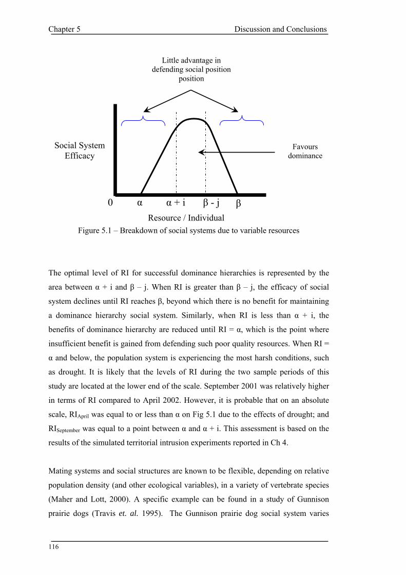
Chapter 5 Discussion and Conclusions
Little advantage in defending social position
position
Figure 5.1 – Breakdown of social systems due to variable resources
The optimal level of RI for successful dominance hierarchies is represented by the
area between α + i and β – j. When RI is greater than β – j, the efficacy of social
system declines until RI reaches β, beyond which there is no benefit for maintaining
a dominance hierarchy social system. Similarly, when RI is less than α + i, the
benefits of dominance hierarchy are reduced until RI = α, which is the point where
insufficient benefit is gained from defending such poor quality resources. When RI =
α and below, the population system is experiencing the most harsh conditions, such
as drought. It is likely that the levels of RI during the two sample periods of this
study are located at the lower end of the scale. September 2001 was relatively higher
in terms of RI compared to April 2002. However, it is probable that on an absolute
scale, RIApril was equal to or less than α on Fig 5.1 due to the effects of drought; and
RISeptember was equal to a point between α and α + i. This assessment is based on the
results of the simulated territorial intrusion experiments reported in Ch 4.
Mating systems and social structures are known to be flexible, depending on relative
population density (and other ecological variables), in a variety of vertebrate species
(Maher and Lott, 2000). A specific example can be found in a study of Gunnison
prairie dogs (Travis et. al. 1995). The Gunnison prairie dog social system varies
Social System Efficacy
Resource / Individual
Favours dominance
α 0 α + i β - j β
116

Chapter 5 Discussion and Conclusions such that monogamy is favoured when resources are uniform regardless of
population density, but this gives way to polygyny when resources become
heterogeneous at intermediate densities, and to polyandry and polygyny at high
densities (Travis et. al., 1995). Thus resource availability affects the breeding
system directly. Additionally, Rodel et al. (2004) identified the proportion of first
time breeders (which have lower success) as another factor that may contribute to
density effects on average reproductive rates in rabbits.
The relationship between social structure and population genetic structure has been
studied extensively. The consensus in the literature is that social systems influence
gene dynamics. Dobson et al. (1998) examined breeding groups and gene dynamics
in a socially structured population of black tailed prairie dogs (Cynomys
ludovicianus). Using allozymes, pedigrees and demographic models they found that
prairie dog breeding groups showed significant genetic differentiation sub-
structuring. Further examples can be found in populations of red howling monkeys
(Alouatta seniculus) that exhibit population genetic structuring as a result of social
groupings as studied by Pope (1992, 1998); and even in humans where native
American populations of Navaho exhibit reduced genetic variability due to
inbreeding effects (Long et al. 1998).
The concept of interference competition in a territorial species was explained by
Lack (1966) as the possibility of an inverse relationship between density and
population growth rate. In the case of the European rabbit, it is likely that
interference competition also affects the breakdown of dominance hierarchies and
hence the social structure (which is effectively the mating system) in high density
populations in arid and semi-arid environments. So rabbit metapopulations are
effectively regulated as a response to habitat heterogeneity. While the European
rabbit has been shown to exhibit flexible behaviour in previous studies (such as
Cowan and Garson, 1985) and the present study to an extent; the influence of social
system variability on genetic structure was not as pronounced as in the above listed
examples. One may argue that the genetic differences between arid and semi-arid
rabbit populations are influenced by the differing social structure caused by habitat
heterogeneity. The environmental constraints on this project resulted in the conduct
of behaviour experiments in different resource periods within the arid region; and
117

Chapter 5 Discussion and Conclusions although differences were observed between control and experimental treatments,
there was not an observed effect on the population genetic structure (given panmictic
results).
These results offer evidence that the flexible behaviour observed in European rabbit
populations in arid Australia is due to phenotypic plasticity (single genotype able to
respond adaptively to local conditions) rather than genotypic polymorphism
(different genotypes adapted to local conditions). Via and Lande (1985) state that
when a population is subdivided, genetic differences may develop among the
subpopulations, perhaps resulting in different life history responses to environmental
changes. Although the arid region is a very large geographic area, the scramble
competition that occurs when resources (and consequently density) are high, ensures
that no genetic differences occur among subpopulations (Fuller et al., 1996, present
study). Clearly, the only way to conduct an absolute test of phenotypic plasticity is to
conduct translocation experiments (Alcock, 1998); which were originally planned as
part of this study (arid vs semi-arid), however, the environmental issues
(drought/disease) and logistics prevented such experiments. The next best thing,
therefore, is to demonstrate phenotypic plasticity by studying the behaviour and
genetics across a small geographic area. This was demonstrated in the present study
through the varied response to control and experimental rabbits.
The genes controlling rabbit behaviour are obviously a complex group rather than a
single gene-single product. Although the genetic portion of this study found evidence
supporting the existence of two ‘systems’ in arid and semi-arid Australia, it is
reasonable to assume that the functional genes controlling behaviour are well
constrained and therefore (statistically) have little chance of rapid mutation
producing a selective advantage. This means that while two discrete population
systems exist in arid and semi-arid Australia, behavioural plasticity, and to a certain
extent, the population genetic structure of rabbits are generally functions of local
environmental conditions (see Hamilton (2003), for further detail on quantifying the
causes of genetic structure in this system). The behaviour of rabbits can certainly
contribute to the population genetic structure, but one can argue that the primary
factor influencing the behaviour patterns themselves is the extant conditions for the
population in question. Therefore, if there is a change in the environmental
118

Chapter 5 Discussion and Conclusions conditions (including habitat connectivity) in either the arid or semi-arid regions, it is
plausible to expect a corresponding change in population genetic structure - only if
the change is severe enough to cause a change in the resources available per
individual, that then alters the benefits associated with defending social position as
described in Fig 5.1.
Brashares and Arcese (2002), demonstrated that Oribi antelope (Ourebia ourebi)
females exhibit variable behaviour in response to availability and quality of food
while males respond to variable distribution and range of females. By identifying
social behaviour variation among contiguous subpopulations in a small geographic
area, the authors established that phenotypic plasticity (rather than genotypic
polymorphism) was the primary mechanism at work (Brashares and Arcese, 2002).
Recent research into ‘candidate genes’ (a gene identified in one organism
hypothesised to influence a similar phenotype in another organism) has provided
further insights into behavioural flexibility – ie. changes in expression of candidate
genes can reveal their contribution to behaviour variation and/or phenotypic
plasticity (Fitzpatrick et al. 2005).
Management of Rabbit Populations in Australia
Although pest management is not the focus of this study, it would be remiss not to
consider the implications of this project on European rabbit management given its
status as a significant vertebrate pest in Australia; and for the same reason, it is not
surprising that much research has been devoted to improving control of this pest.
Early control efforts were aimed at preventing dispersal through the use of rabbit
proof fences, however, these were largely ineffectual given the size of the area of
land involved and the fact that often the “rabbit front” passed the fence before the
fence was even completed. Other methods involved the use of “rabbiters”, however,
as the meat and pelt industries grew, so did the conflict of interests for rabbiters –
and realistically, shooting, netting, ferreting, and trapping were never effective as
widespread management tools, much less for eradicating the rabbit in Australia.
It is accepted by most biologists that the rabbit has become a permanent inhabitant of
Australia, and therefore, the focus needs to be on effective population management,
119

Chapter 5 Discussion and Conclusions rather than complete eradication (Williams et al. 1995). Methods such as baiting,
mechanical ripping of warrens, and netted fencing, are particularly useful for
localised control, however, the success of any overall control program will depend
on the population levels in areas adjacent to those under treatment because it is
impossible to apply localised control everywhere. If there is a population “source” or
“refuge” located nearby, then localised management efforts are likely to be
undermined by dispersal from areas adjacent to areas where populations are being
controlled.
The introduction of biological control through myxomatosis was initially very
effective in Australia, as the disease spread via rabbit to rabbit contact (via fleas),
and required little human action other than release of the disease. The problem with
myxomatosis was that resistance to the disease gradually increased to the point that
very large populations of rabbits developed once more. In the mid 1990’s, the rabbit
calici virus was identified as a new form of biological control agent for rabbits and as
such, has been applied widely around Australia with many release sites across the
country (Kovalski, 1998). To date, the combined effect of the virus and significant
drought conditions have resulted in some of the lowest rabbit population densities
seen for many decades.
One of the problems associated however, with developing successful management
strategies, is the perception that arises from short term success. The general
population and government agencies, often view a significant reduction in population
size of a pest as the successful conclusion to a management program; whereas in
reality it is only the beginning and initial successes must be followed by funding and
efforts to sustain treatments. The most successful management efforts are a
combination of treatments in what amounts to an integrated pest management
approach across areas of land that can be viewed as effective management units
(Holder et al. 2004).
The mechanical ripping of warrens is highly effective in preventing recolonisation of
an area that has been cleared of rabbits (Brennan, pers comm), and is an ideal follow
up treatment in arid and semi-arid areas (Edwards et al. 2002). While the cost is
high, both environmentally and economically, it is efficient provided the terrain is
120

Chapter 5 Discussion and Conclusions conducive to the use of large earthmoving equipment. Areas with greater tree
coverage, however, cannot be treated in this way. Chemical treatment through the
use of baits, is also expensive and can cause death of non-target species (McIlroy,
1983; Choquenot et al. 1990), however, it may present as a viable control option to a
landholder potentially facing a plague of rabbits.
Biological controls represent potentially one of the most cost (and effort) effective
methods for managing any pest. This is possible if the biological control agent can
establish itself in the wild and spread through populations naturally after initial
introduction. Myxomatosis and rabbit calici virus were successful biological control
agents that have persisted in populations over many generations (Cooke et al. 2004).
Development of resistance is a major problem that often arises when diseases are
used as biological control agents. While myxomatosis is established in Australian
populations, there is also a high level of resistance that has evolved since it was first
released, resulting in declining rabbit mortality rates (Kerr and McFadden, 2002). It
also means that new viral strains must be developed constantly in order to maintain
control. Similarly, while the rabbit calci virus has been effective in arid and semi-
arid environments since its release in 1996, it is likely that resistance will evolve in
time, and when it does, rabbit population sizes will probably increase once more.
The importance of an integrated approach to management of rabbit populations is
highlighted by the way that the effects of drought conditions have combined with the
effects of rabbit calici virus to reduce the population sizes in arid and semi-arid
Australia (Story et al. 2004). In some cases, local control efforts have included
ripping of old warren systems to reduce the risk of recolonisation, and laying of baits
to target residual rabbits surviving in refugia.
Understanding the behavioural attributes of rabbit populations can also be of major
use in developing better pest management strategies in the future that have a
biological control component provided the vector depends on some degree of rabbit
to rabbit contact to enable effective transmission of the disease. The current study
has identified the potential for rabbits to exhibit differential amounts of aggressive
behaviour in arid environments as a response to regional environmental conditions,
which may impact the efficiency of disease vectors in certain situations. If population
121

Chapter 5 Discussion and Conclusions densities are very high, and the normal pattern of the rabbit territorial social system
are “short-circuited”, then it is possible the ensuing scramble competition would be
far more conducive to spreading diseases than if dispersing rabbits were continually
successfully excluded from colonising new patches. Lombardi et al. (2003) presented
evidence collected in Mediterranean environments to suggest that mortality by
disease may be linked to levels of rabbit aggression. Therefore, landholders and
management planners, may want to consider the behavioural status of their target
populations as part of their strategic plans. That is not to say that biological control
cannot be used under normal territorial conditions, however, it does mean a more
judicious approach to the application of disease agents may be required. Biological
control agents are likely to be more effective when released from multiple sites in
regions where territoriality is high and or dispersal is relatively low; a good example
of this method was observed in the Mitchell region in 1996 (eastern / semi-arid area
in this project). The Department of Natural Resources used the sites shown in figure
5.2 for the release of rabbit calici virus - the area was previously shown to have low
natural levels of rabbit dispersal (Fuller, 1995). If the virus was not released in such a
widespread manner, it is doubtful whether the effects would have been as dramatic.
Figure 5.2 – Rabbit calci virus release, Mitchell, 1996 (source: DNRM)
122

Chapter 5 Discussion and Conclusions
Future Directions of Research and Conclusion
Although the European rabbit is well researched, there are several research
opportunities available to address the knowledge gaps that have been identified in
this project, which would assist management and conservation efforts in the rabbit’s
introduced and native ranges respectively.
The drought conditions and effectiveness of the calci virus program in the semi-arid
region forced the modification of the experimental design used here so that
behaviour experiments were conducted solely in arid conditions on population sizes
at low levels. An interesting study would be to conduct identical experiments in the
semi-arid and arid regions when population sizes are relatively large. However, this
is unlikely to be possible for at least ten to twenty years and possibly longer, given
the current effects of drought and successful implementation of management
programs targeting rabbit refuge areas (Berman, 2004).
Further research opportunities also include quantifying the population size (or
Resource / Individual level) at which dominance hierarchies may break down – i.e.
under what environmental conditions and population densities does the “short-
circuit” of normal rabbit social systems occur? The question may be answered
through the use of computer simulation modelling and direct population size
estimations in the field when threshold densities are achieved.
The aim of this research project was to assess whether wild rabbits adjust their
behavioural patterns as a response to variation in environmental factors, that leads to
observable differences in population genetic structure. Consequently there are two
major outcomes of this project:
1. A difference in population genetic structure was observed at the individual level
between arid and semi-arid regions which supports the findings of Fuller (1995)
and Fuller et. al. (1996, 1997) that identified regional differences using
maternally inherited markers.
2. Differences in the aggressive response to known vs unknown rabbits were
identified in parts of the arid region, which together with the effects of habitat
123

Chapter 5 Discussion and Conclusions
heterogeneity and connectivity (Hamilton, 2003) may explain the observed
differences in population genetic structure.
A major outcome of this study would be if the findings could be utilised to improve
management strategies, particularly those reliant on biological vectors, in countries
where Oryctolagus cuniculus is a significant pest species. Additionally, the outcomes
from this project may assist in better conservation practices in the native range of
southern Europe where the rabbit is an endangered species.
124

APPENDIX 1 Description of rabbit behaviours (modified from Webb, 1988) 1. Grazing Down: Feeding with head lowered near vegetation. 2. Grazing Up: Head raised away from vegetation but still chewing. 3. Resting Alert: Head up with ears erect, but not chewing. 4. Alert: Sitting upright with front legs raised off ground, ears erect. 5. Resting: Inactive with ears flattened, eyes partially or wholly closed. Lying with
legs tucked beneath, lying on side with white belly fur exposed. 6. Grooming: Licking or scratching the fur. Rabbits may flick the front paws
rapidly up and down (“air box”) before grooming the head and ears. 7. Moving: Either slow hops while feeding, or rapid running in response to
disturbance from people, predators etc. 8. Chasing: One individual rapidly pursuing another. The chasing animal may
attempt to bite the fleeing animal if it gets close enough. 9. Displacement: One individual moves toward another resulting in the latter
moving away. Sometimes accompanied by a threat with the head thrust forward and ears flattened.
10. Sexual Following: Male follows female at a slow pace, often stops to sniff the ground where the female been.
11. Circling: Male hops around female. Often accompanied by behaviours 12 and 13. (NOTE: Circling used in this report refers to local animals circling the cage in which the decoy animal was located.)
12. Urine Spray: Male sprays urine over another individual while leaping over or past it. Usually target animal is a female, occasionally a subordinate male.
13. Tail Flagging: Individual hops with rather stiff looking hind legs and raises tail to expose white underside. This behaviour is performed by both sexes during aggressive interactions, although more commonly by males. It is also seen when males are circling females.
14. Tail Wagging: Tail lowered so that black topside is visible and wagged rapidly from side to side. Performed by females towards courting males and towards their own young.
15. Bowing: One individual lowers head and flattens ears as another approaches. Usually performed by females toward males which then proceed to sniff, groom, and chin mark on the female’s head or move around behind the female and attempt to mount. Occasionally performed by a subordinate individual to a higher ranking animal of the same sex, and also by juveniles to adults.
16. Chin Marking: Rubbing the chin over an object, releasing a secretion from the chin (sub mandibular) gland (Myktowycz 1968)
17. Paw Scrapping: Rapid scratching of the ground with the fore paws. Can be either to expose roots during foraging or it is seen before males chin mark, defecate, or urinate during patrolling and territorial marking. Also performed by males during agnostic encounters (see below).
18. Parallel Running and Paw Scrapping: Males (and sometimes females) of neighbouring social groups run in parallel along the territory boundary, occasionally stopping to paw scrape.
19. Fighting (“Aggressive Leaping”): Two individuals simultaneously jump towards each other. They pass in the air, land, and then repeat the process in the opposite direction. Usually these jumping fights are brief, 1-5 leaps. Mainly seen
125

between males on territory boundaries, occasionally between two females. Individuals from the same group sometimes interact in this way if they have come into close contact “unintentionally” eg. If one of them is engaged in a rapid chase.
20. Fighting (involving close contact): Individuals locked together in combat comprising vigorous scratching with the hind legs and biting.
126

Bibliography Bibliography
Akiyama, S., Yasuda, K., Arimoto, T., Tawara, Y. (1995). Underwater observation
of fish behaviour to trolling line. Nippon Suisan Gakkaishi-Bulletin of the
Japanese Society of Scientific Fisheries. 61(5): 713-716.
Alcock, J. (1984). Animal Behaviour: An Evolutionary Approach. Sunderland,
USA, Sinauer Associates.
Alcock, J. (1998). Animal Behaviour: An Evolutionary Approach.6th Edition.
Boston, USA, Sinauer Associates.
Alonso, J. C., Alonso, J. A., Bautista, L. M., Munoz, P.R. (1995). “Patch use in
cranes: A field test of optimal foraging predictions.” Animal Behaviour
49(5): 1367-1379.
Berman, D. (2001). Personal Communication.
Berman, D. (2004). Bulloo bunnies bite the dust. Mulga Line Newsletter Dec
'03/Jan '04, Issue 11. http://www.dpi.qld.gov.au/mulgaline/14570.html
accessed on 09 June 2004.
Bonnell, M. L. and Selander, R. K. (1974). “Elephant seals: Genetic variation and
near extinction.” Science 184: 908-909.
Bowland, A. E. and Perrin, M. R. (1995). “Temporal and spatial patterns in blue
duikers Philatomba monticola and red duikers Cephalophus natalensis.”
Journal of Zoology London 237(3): 487-498.
Bozinovic, F., Vasquez, R. (1999). Patch use in a diurnal rodent: Handling and
searching under thermoregulatory costs. Functional Ecology. 13(5): 602-610.
127

Bibliography Brashares, J.S. and Arcese, P. (2002). Role of forage, habitat and predation in the
behavioural plasticity of a small African antelope. Journal of Animal Ecology
71: 626-638.
Broders, H.G., Mahoney, S.P., Montevecchi, W.A., Davidson, W.S. (1999).
Population genetic structure and the effects of founder events on the genetic
variability of moose, Alces alces, in Canada. Molecular Ecology. 8: 1309-
1315.
Chesser, R., Sugg, D., Rhodes, O., Novak, J., and Smith, M. (1993). Evolution of
mammalian social structure. Acta Theriologica 38(2): 163-174.
Chesser, R. (1998). Relativity of behavioural interactions in socially structured
populations. Journal of Mammology 79(3): 713-724.
Choquenot, D., Kay, B., Lukins, B. (1990). An evaluation of warfarin for the control
of feral pigs. Journal of Wildlife Management 54: 353-359.
Clarke, M. F. (1984). “Cooperative breeding by the Australian bell miner Manorina
melanophrys Latham: a test of kin selection theory.” Behavioural Ecology
and Sociobiology 14: 137-146.
Clarke, M. F. (1989). “The pattern of helping in the bell minor (Manorina
melanophrys).” Ethology 80: 292-306.
Clarke, M. F. and Fitz-Gerald, G. F. (1994). “Spatial organisation of the cooperative
breeding bell miner Manorina melanophrys.” Emu 94: 96-105.
Corbet, G. B. (1986). “Relationships and origins of the European lagomorphs.”
Mammal Review 16: 105-110.
Cooke, B. (2001). Personal Communication.
128

Bibliography Cooke, B., Chapuis, J., Magnet, V., Lucas, A., Kovaliski, J. (2004). Potential use of
myxoma virus and rabbit haemorrhagic disease virus to control feral rabbits
in the Kerguelen Archipelago. Wildlife Research 31(4): 415-420.
Cowan, D.P. (1983). Aspects of the behavioural ecology of a free living population
of the European wild rabbit, Oryctolagus cuniculus L. in Southern England.
PhD Thesis. Royal Holloway College.
Cowan, D. P. (1987a). “Aspects of the social organisation of the European wild
rabbit (Oryctolagus cuniculus).” Ethology 75: 197-210.
Cowan, D. P. (1987b). “Group living in the European rabbit, Oryctolagus cuniculus:
mutual benefit or resource localisation.” Journal of Animal Ecology 56: 779-
795.
Cowan, D. P. and Garson, P. J. (1985). Variations in the social structure of rabbit
populations: causes and demographic consequences. Behavioural
Ecology:ecological consequences of adaptive behaviour. R. M. Sibly and R.
H. Smith. Oxford, Blackwell Scientific Publications.
Daly, J. C. (1979). The ecological genetics of the European wild rabbit (Oryctolagus
cuniculus) in Australia. Canberra, Australian National University.
Daly, J. C. (1981). “Effects of social organisation and environmental diversity on
determining the genetic structure of a population of the wild rabbit,
Oryctolagus cuniculus.” Evolution 35(4): 689-706.
Deforce, E., Deforce, C., Lindeman, P. (2004). Phrynops gibbus (Gibba turtle).
Herpetological Review 35 (1): 55-56.
DeYoung, R.W., Demarais, S., Honeycutt, R.L., Rooney, A.P., Gonzales, R.A., Gee,
K.L. (2003). Genetic consequences of white-tailed deer (Odocoileus
virginianus) restoration in Mississippi. Molecular Ecology 12: 3237-3252.
129

Bibliography
Dobson, F. (1998). Social structure and gene dynamics in mammals. Journal of
Mammology. 79(3): 667-670.
Dobson, F., Chesser, R., Hoogland, J., Sugg, D., Foltz, D. (1998). Breeding groups
and gene dynamics in a socially structured population of prairie dogs. Journal
of Mammalogy. 79: 671 - 680.
Ebenhard, T. (1991). “Colonization in metapopulations: a review of theory and
observations.” Biological journal of the linnean society 42: 105-121.
Edwards, G., Dobbie, W., Berman, D. (2002). Warren ripping: Its impacts on
European rabbits and other wildlife of central Australia amid the
establishment of rabbit haemorrhagic disease. Wildlife Research 29(6): 567-
575.
Fallows, M.S. (1988). Rabbit grazing: An inter-disciplinary approach. PhD Thesis.
University of East Anglia.
Fitzpatrick, M., Ben-Shahar, Y., Smid, H., Vet, L., Robinson, G., Sokolowski, M.
(2005). Candidate genes for behavioural ecology. Trends in Ecology and
Evolution 20(2): 96-104.
Flux, J. E. C. (1994). World Distribution. The European Rabbit, The history and
biology of a successful colonizer. H. V. Thompson and C. M. King. New
York, Oxford University Press: 8-21.
Frankham, R. (1996). Relationship of genetic variation to populations size in
wildlife. Conservation Biology 10, 1500-1508.
Fullagar, P. J. (1981). Methods for studying the behaviour of rabbits in a 33-ha
enclosure at Canberra and under natural conditions at Calindry, New South
130

Bibliography
Wales. Proceedings of the world lagomorph conference, Guelph, Ontario.
1979. R. Myers and C. D. MacInnes.
Fuller, S. J., Mather, P.B., Wilson, J.C. (1996). “Limited genetic differentiation
among wild Oryctolagus cuniculus L. (rabbit) populations in arid eastern
Australia.” Heredity 77: 138-145.
Fuller, S. J., Wilson, J. C., Mather, P.B. (1997). “Patterns of differentiation among
wild rabbit populations Oryctolagus cuniculus L. in aridand semiarid
ecosystems of north-eastern Australia.” Molecular Ecology 6: 145-153.
Goodman, S.J., Tamate, H.D., Wilson, R. (2001). Bottlenecks, drift, and
differentiation: the population structure and demographic history of sika deer
(Cervus nippon) in the Japanese archipelago. Molecular Ecology 10: 1357-
1370.
Goudet, J., (1995). Fstat version 1.2: a computer program to calculate Fstatistics. Journal of Heredity. 86(6): 485-486.
Grant, J. W. A. (1993). “Whether or not to defend? The influence of resource
distribution.” Marine Behaviour and Physiology 23: 137-153.
Greaves, L., Wedderburn, M. (1995). Comparison of the behaviour of goats and
sheep on and eroded hill pasture. Applied Animal Behaviour Science. 42(3):
207-216.
Gross, M. R. and MacMillan, A. M. (1981). “Predation and the evolution of colonial
nesting in bluegill sunfish (Lepomis macrochirus).” Behavioural Ecology and
Sociobiology 8: 163-174.
Hamilton, W. D. (1964). “The genetical evolution of social behaviour. I, II.” Journal
of Theoretical Biology 7: 1-52.
131

Bibliography Hamilton, G. (2003). The influence of habitat heterogeneity on patterns of
connectivity in rabbit populations in southern Queensland. PhD thesis.
Queensland University of Technology.
Hanski, I. and Gilpin, M. (1991). Metapopulation dynamics: brief history and
conceptual domain. Biological journal of the Linnean Society 42: 3-16.
Hansson, L. (1991). “Dispersal and connectivity in metapopulations.” Biological
journal of the Linnean society 42: 89-103.
Hardy, C., D. Casane, et al. (1994). “Ancient DNA from Bronze Age bones of
European rabbit (Oryctolagus cuniculus).” Experientia 50(6): 564-70.
Harrison, S. (1991). “Local extinction in a metapopulation context: an empirical
evaluation.” Biological Journal of the Linnean Society 42: 73-88.
Hartl D. (1988). A primer of population genetics. 2nd Ed. Sinauer Associates Inc.
Mass. USA.
Hartl, D. L. and Clark, A. G. (1997). Principles of population genetics. Sunderland,
Sinauer Associates Inc.
Hau, M.; Stoddard, S.; Soma, K. (2004). Territorial aggression and hormones during
the non-breeding season in a tropical bird. Hormones and Behaviour 45 (1):
40-49.
Hedrick, P. W. (1999). Genetics of populations. London, Jones and Bartlett.
Hedrick, P. W. (2000). Genetics of populations, 2nd Edition, Sudbury, Jones and
Bartlett.
132

Bibliography Henderson, B.A. (1979). Regulation of the size of breeding population of the
European Rabbit, Oryctolagus cuniculus, by social behaviour. Journal of
Applied Ecology 16: 383-392.
Holder, K., Montgomerie, R., Friesen, V. (2004). Genetic diversity and management
of Nearctic rock ptarmigan (Lagopus mutus). Canadian Journal of Zoology
82(4): 564-575.
Hume, F., Pemberton, D., Gales, R., Brothers, N., Greenwood, M. (2002). Trapping
and relocating seals from salmonid fish farms in Tasmania, 1990-2000: Was
it a success? Papers and Proceedings of the Royal Society of Tasmania 136:
1-6.
Ims, R. A. (1987). Responses in spatial organisation and behaviour to manipulations
of the food resource in the vole Clethrionomys rufocanus. Journal of Animal
Ecology 56: 585-596.
Jolly, S. E., Spurr, E. B., Cowan, P.E. (1999). “Social dominance and breeding
success in captive brushtail possums, Trichosurus vulpecula.” New Zealand
Journal of Zoology. March 26(1): 21-25.
Kerr, P., McFadden, G. (2002) Immune responses to myxoma virus. Viral
Immunology 15(2): 229-246.
Kimura, M. and Weiss, G. H. (1964). “The stepping stone model of population
structure and the decrease of genetic correlation with distance.” Genetics 49:
561-576.
Kovalski, J. (1998). Monitoring the spread of rabbit hemorrhagic disease virus as a
new biological agent for control of wild European rabbits in Australia.
Journal of Wildlife Diseases 34(3): 421-428.
133

Bibliography Krebs, C. J. (1994). Ecology: The experimental analysis of distribution and
abundance. New York, HarperCollins College Publishers.
Kutt, A. (2003). The Spinifexbird Eremiornis carteri in the Desert Uplands
Bioregion, north-central Queensland: A geographic isolate or a nomadic
metapopulation? Australian Zoologist 32(2): 246-251.
Lack, D. (1966). Population studies of birds. Clarendon Press, Oxford.
Landergren, P. (1999). Spawning of anadromous rainbow trout, Oncorhynchus
mykiss (Walbaum): A threat to sea trout, Salmo trutta L., populations?
Fisheries Research (Amsterdam). 40 (1): 55-63.
Levins, R. A. (1969). “Some demographic and genetic consequences of
environmental heterogeneity for biological control.” Bulletin of the
entomological society of America 15: 237-240.
Lockley, R.M. (1954) The private life of a rabbit. Transworld Publishers Ltd.
(Corgi). London.
Lombardi, L., Fernandez, N., Moreno, S., Villafuerte, R. (2003). Habitat related
differences in rabbit (Oryctolagus cuniculus) abundance, distribution, and
activity. Journal of Mammology 84: 26-36.
Long, J., Romero, F., Urbanek, M., Goldman, D. (1988). Mating patterns and gene
dynamics of an American indian population isolate. Journal of Mammalogy
79: 681-691.
Loo, W., Arthur, C. (1987). “Nonrandom allele associations between unlinked
protein loci: are the allotypes of the immunoglobulin constant regions
adaptive?” Proceeding of the National Academy of Science USA 84: 3075-
3079.
134

Bibliography Lurzs, P. W. W., Garson, P. J., Wauters, L.A. (1997). “Effects of temporal and
spatial variation in habitat quality on red squirrel dispersal behaviour.”
Animal Behaviour 54(2): 427-435.
Maher, C. R., Lott, D. F. (2000). A review of ecological determinants of territoriality
within vertebrate species. American Midland Naturalist 143: 1-29.
Marra, P. (2000). The role of behavioral dominance in structuring patterns of habitat
occupancy in a migrant bird during the nonbreeding season. Behavioral
Ecology 11(3): 299-308.
McIlroy, J. (1983). The sensitivity of animals to 1080 poison. V. The sensitivity of
feral pigs, Sus scrofa, to 1080 and its implications for poisoning campaigns.
Australian Wildlife Research 10: 139-148.
Mougel, F., J.-C. Mounolou, Monnerot, M. (1997). “Nine polymorphic microsatellite
loci in the rabbit, Oryctolagus cuniculus.” Animal Genetics 28: 58-71.
Myers, K., Parer, I., Wood, D., Cooke, B.D. (1994). The rabbit in Australia. The
European Rabbit, The history and biology of a successful colonizer. H. V.
Thompson and C. M. King. New York, Oxford University Press: 108-157.
Mykytowycz, R., (1958). Social behaviour of an experimental colony of wild rabbits,
Oryctolagus cuniculus (L.) I. Establishment of the colony. CSIRO Wildlife
Research 3: 7-25.
Mykytowycz, R., (1959). Social behaviour of an experimental colony of wild rabbits,
Oryctolagus cuniculus (L.) II. First breeding season. CSIRO Wildlife
Research 4: 1-13.
Mykytowycz, R., (1960). Social behaviour of an experimental colony of wild rabbits,
Oryctolagus cuniculus (L.) III. Second breeding season. CSIRO Wildlife
Research 5: 1-20.
135

Bibliography
Mykytowycz, R., Hesterman, E. R., Purchase, D. (1960). “Techniques employed in
catching rabbits, Oryctolagus cuniculus, in an experimental enclosure.”
CSIRO Wildlife Research 5: 85-86.
Mykytowycz, R. and Gambale, S. (1965). A study of the inter-warren activities and
dispersal of wild rabbits, Oryctolagus cuniculus (L.), living in a 45acre
paddock. CSIRO Wildlife Research 10: 111-123.
Mykytowycz, R. and Fullagar, P.J. (1973). Effect of social environment on
reproduction in the rabbit, Oryctolagus cuniculus (L.). Journal of
Reproduction and Fertility, Supplement 19: 503-522.
Nei, M., Maruyama, T., Chakraborty, R. (1975). The bottleneck effect and genetic
variability in populations. Evolution 29: 1-10.
Nihei, Y. (1995). Variations of behaviour of carrion crows Corvus corone using
automobiles as nutcrackers. Japanese Journal of Ornithology 44(1): 21-35.
O'Brien, S. J., Wildt, D. E., Bush, M., Caro, T.M., Fitzgibbon, C., Aggundey, I.,
Leakey, R.E. (1987). “East African cheetahs: Evidence for two population
bottlenecks.” Proceedings of the National Academy of Sciences USA 84:
508-511.
Painter, J. N., Crozier, R. H., Poiani, A., Robertson, R.J., Clarke, M.F. (2000).
“Complex social organisation reflects genetic structure and relatedness in the
cooperatively breeding bell minor, Manorina melanophrys.” Molecular
Ecology 9: 1339-1347.
Parer, I. (1982). “Dispersal of the wild rabbit, Oryctolagus cuniculus, at Urana in
New South Wales.” Australian Wildlife Research 9: 427-441.
136

Bibliography Parer, I. and Fullagar, P. J. (1986). “Biology of rabbits, Oryctolagus cuniculus, in
southern Queensland.” Australian Wildlife Research 16: 563-568.
Partridge, L. and Sgro, C. M. (1998). “Behavioural genetics: Molecular genetics
meets feeding ecology.” Current Biology 8(1): R23-R24.
Peakall, R., Smouse, P.E., 2006. GENALEX 6: genetic analysis in Excel. Population
genetic software for teaching and research. Molecular Ecology Notes 6, 288-
295.
Petren, K., Case, T. (1998). Habitat structure determines competition intensity and
invasion success in gecko lizards. Proceedings of the National Academy of
Sciences of the United States of America. 95 (20): 11739-11744.
Pierce, B. M., and Bleich, V.C. (1998). “Timing of feeding bouts of Mountain
Lions.” Journal of Mammalogy 79(1): 222-226.
Piper, W., Tischler, K., Klich, M. (2000). Territory acquisition in loons: The
importance of take-over. Animal Behaviour 59 (2): 385-394.
Polziehn, R.O., Hamr, J., Mallory, FF, Strobek, C. (2000). Microsatellite analysis of
North American wapiti (Cervus elaphus) populations. Molecular Ecology 9:
1561-1576.
Pope, T. (1992). The influence of dispersal patterns and mating systems on genetic
differentiation within and between populations of the red howling monkey
(Alouatta seniculus). Evolution 46: 1112-1128.
Pope, T. (1998). Effects of demographic change on group kin structure and gene
dynamics of red howling monkey populations. Journal of Mammalogy 79:
692-712.
137

Bibliography Pough, F. H., Heiser, J. B., McFarland, W.N. (1989). Vertebrate Life. New York,
Macmillan Publishing Company.
Queney, G., Ferrand, N., Marchandeau, S., Azevedo, M., Mougel, F., Branco, M.,
Monnerot, M. (2000). “Absence of a genetic bottleneck in a wild rabbit
(Oryctolagus cuniculus) population exposed to a severe viral epizootic.”
Molecular Ecology 9: 1253-1264.
Queney, G., Ferrand, N., Marchandeau, S., Azevedo, M., Mougel, F., (2001).
“Stationary distributions of microsatellite loci between divergent population
groups of the European rabbit (Oryctolagus cuniculus).” Molecular Biology
and Evolution 18(12): 2169-2178.
Raymond, M. and Rousset, F. GENEPOP (version 1.2) (1995): Population genetics
software for exact tests and ecumenicism. Journal of Heredity 86: 248-249.
Reece, C. (1985) Aspects of reproduction in the European rabbit, O. cuniculus (L.).
PhD Thesis. University of East Anglia.
Richardson, B. J. (1980). “Ecological genetics of the wild rabbit in Australia. III. A
comparison of the microgeographical distribution of alleles in two different
environments.” Australian Journal of Biological Science 33: 385-391.
Richardson, B. J. (1981). The genetic structure of rabbit populations. Proceedings of
the world lagomorph conference, Guelph, August 1979. K. Myers and M.
C.D. Guelph, University of Guelph: 37-52.
Richardson, B. J., R. A. Hayes, Wheeler, S., Yardin, M. (2002). “Social structures,
genetic structures and dispersal strategies in Australian rabbit (Oryctolagus
cuniculus) populations.” Behavioural Ecology and Sociobiology 51: 113-121.
Richardson, B. J., Rogers, P. M. (1980). “Ecological genetics of the wild rabbit in
Australia. II. Protein variation in British, French and Australian rabbits and
138

Bibliography
the geographical distribution of the variation in Australia.” Australian Journal
of Biological Science 33: 371-383.
Rico, C., Rico, I., Webb, N., Smith, S., Bell, D., Hewitt, G. (1994). “Four
polymorphic microsatellite loci for the European wild rabbit, Oryctolagus
cuniculus.” Animal Genetics 25: 325.
Robb, S. E. and Grant, J. W. A. (1998). “Interactions between the spatial and
temporal clumping of food affect the intesity of aggression in Japanese
medaka.” Animal Behaviour 56: 29-34.
Roberts, R. C. (1979). “The evolution of avian food-storing behaviour.” The
American Naturalist 114(3): 418-438.
Rodel, H., Bora, A., Kaiser, J., Kaetzke, P., Khaschei, M., von Holst, D. (2004).
Density dependent reproduction in the European rabbit: a consequence of
individual response and age dependent reproductive performance. Oikos 104:
529-539.
Rolls, E. C. (1984). They all ran wild : the animals and plants that plague Australia.
London ; Sydney, Angus & Robertson.
Ross, J. and M. F. Sanders (1984). “The development of genetic resistance to
myxomatosis in wild rabbits in Britain.” Journal of Hygiene 92(3): 255-61.
Ryberg, W.A., Fitzgerald, L.A., Honeycutt, R.L., Cathey, J.C. (2002). Genetic
relationships of American alligator populations distributed across different
ecological and geographic scales. Journal of Experimental Zoology (Mol Dev
Evol) 294: 325-333.
Seindensticker, J. C., Hornocker, M. G., Wiles, W.V., Messick, J.P. (1973).
“Mountain lion social organization in the Idaho Primitive Area.” Wildlife
Monographs 35: 1-60.
139

Bibliography
Shaffer, M. L. (1981). “Minimum population sizes for species conservation.”
Bioscience 31: 131-134.
Sherry, D. (1984). “Food storage by blackcapped chickadees; memory for the
location and contents of caches.” Animal Behaviour 32: 451-64.
Slatkin, M. (1994). Gene flow and population structure. Ecological Genetics. L. A.
Real. Princeton, Princeton University Press.
Smith, C. C. and Reichman, O. J. (1984). “The evolution of food caching by birds
and mammals.” Annual Review of Ecology and Systematics 15: 329-51.
Southern, H E N. (1948). Sexual and aggressive behaviour in the wild rabbit.
Behaviour. 1: 173-194.
StatSoft, Inc. (2001). STATISTICA (data analysis software system), version 6.
www.statsoft.com.
StatSoft, Inc. (2006). Electronic Statistics Textbook. Tulsa, OK: StatSoft. WEB:
http://www.statsoft.com/textbook/stathome.html.
Stodart, E. and Parer, I. (1988). Colonisation of Australia by the rabbit Oryctolagus
cuniculus (L.). Canberra, CSIRO Division of Wildlife and Ecology.
Story, G., Berman, D., Palmer, R., Scanlan, J. (2004). The impact of rabbit
haemorrhagic disease on wild rabbit (Oryctolagus cuniculus) populations in
Queensland. Wildlife Research 31(2): 183-193.
Sunnucks, P. (1998). Avoidance of novel objects by rabbits (Oryctolagus cuniculus).
Wildlife Research 25 (3): 273-283.
140

Bibliography Surridge, A. K., D. J. Bell, Rico, C., Hewitt, G. (1997). “Polymorphic microsatellite
loci in the European rabbit (Oryctolagus cuniculus) are also amplified in
other lagomorph species.” Animal Genetics 28: 302-305.
Surridge, A. K., D. J. Bell, Hewitt, G. (1999). “From population structure to
individual behaviour: genetic analysis of social structure in the European wild
rabbit (Oryctolagus cuniculus).” Biological Journal of the Linnean Society.
68(1-2): 57-71.
Surridge, A. K., Bell, D., Ibrahim, K., Hewitt, G. (1999). “Population structure and
genetic variation of European wild rabbits (Oryctolagus cuniculus) in East
Anglia.” Heredity. 82(Part 5): 479-487.
Surridge, A. K., Ibrahim, K., Bell, D., Webb, N., Rico, C., Hewitt, G. (1999). “Fine-
scale genetic structuring in a natural population of European wild rabbits
(Oryctolagus cuniculus).” Molecular Ecology 8(2): 299-307.
Taylor, A. C., Cowan, P. E., Fricke, B.L., Cooper, D.W. (2000). “Genetic analysis
of the mating system of the common brushtail possum, Trichosurus
vulpecula,in New Zealand farmland.” Molecular Ecology 9(7): 869-879.
Tinbergen, N. (1964). Social behaviour in animals. London, Chapman & Hall.
Travis, S. E., Slobodchikoff C. N., Kiem P. (1995). Ecological and demographic
effects on intraspecific variation in the social system of prairie dogs. Ecology
76: 1794-1803.
Trivers, R. L. (1972). Parental investment and sexual selection. Sexual Selection and
the Descent of Man. C. B.G. Chicago, Aldine Press: 136-179.
Tuyttens, F., MacDonald, D., Delahay, R., Rogers, L., Mallinson, P., Donnelly, C.,
Newman, C. (1999). Differences in trappability of European badgers Meles
141

Bibliography
meles in three populations in England. Journal of Applied Ecology 36 (6):
1051-1062.
van Haeringen, W. A., den Bieman, M., Van Zutphen, L., Van Lith, H. (1996).
“Polymorphic microsatellite DNA markers in the rabbit (Oryctolagus
cuniculus).” Journal of Experimental Animal Science 38(2): 49-57.
Webb, N.J. (1988). Genetic analysis of social structure in the European wild rabbit,
Oryctolagus cuniculus (L.). PhD Thesis. University of East Anglia.
Webb, N. J., Ibrahim, K. M., Bell, D.J., Hewitt, G.M. (1995). “Natal dispersal and
genetic structure in a population of the European wild rabbit (Oryctolagus
cuniculus).” Molecular Ecology 4(2): 239-47.
Wells, K. D. (1977). “The social behaviour of anuran amphibians.” Animal
Behaviour 25: 666-693.
White, B., Dew, S., Prather, J., Stearns, M., Schneider, E., Taylor, S. (2000). Chest-
rubbing in captive woolly monkeys (Lagothrix lagotricha). Primates 41(2):
185-188.
Whitlock, M. C. and McCauley, D. E. (1999). “Indirect measures of gene flow and
migration: Fst not equal to 1/(4Nm + 1).” Heredity 82: 117-125.
Widowski, T., Duncan, I. (1996). Laying hens do not have a preference for high-
frequency versus low-frequency compact fluorescent light sources. Canadian
Journal of Animal Science. 76(2): 177-181.
Wiklund, C. G. and Village, A. (1992). Sexual and seasonal variation in territorial
behaviour of Kestrals (Falco tinnunculus). Animal Behaviour 43 (5): 823-
830.
142

Bibliography Williams, G. C. (1966). Adaptation and Natural Selection, a critique of some current
Evolutionary thought. Princeton, Princeton University Press.
Williams, K., Parer, I., Conman, B., Burley, J., Braysher, M. (1995). Managing
Vertebrate Pests. Rabbits. Canberra, Australian Government Publishing
Service.
Wilson, J.C., Fuller, S.J., Mather P.B. (2002). Formation and maintenance of discrete
wild rabbit (Oryctolagus cuniculus) population systems in arid Australia:
Habitat heterogeneity and management implications. Austral Ecology 27:
183-191.
Winskill L., Waran, N., Young, R. (1996). The effect of a foraging device (a
modified 'Edinburgh Foodball') on the behaviour of the stabled horse.
Applied Animal Behaviour Science. 48(1-2): 25-35.
Wood, D. H. (1980). “The demography of a rabbit population in an arid region of
New South Wales, Australia.” Journal of Animal Ecology 49: 55-79.
Wrazen, J. A. and Wrazen, L. A. (1982). “Hoarding, body mass dynamics, and torpor
as components of survival strategy of the eastern chipmunk.” Journal of
Mammalogy 63: 63-72.
Wright, S. (1931). “Evolution in Medelian populations.” Genetics 16: 97-159.
Wright, S. (1943). “Isolation by distance.” Genetics 28: 114-138.
Wright, S. (1951). “The genetical structure of populations.” Annals of eugenics 15:
323-354.
Zenger, K.R., Richardson, B.J., Vachot-griffin, A. (2003). A rapid population
expansion retains genetic diversity within European rabbits in Australia.
Molecular Ecology 12: 789-794.
143
Recommended