Discrete and continuous SIS epidemic models: a

unifying approach

Fabio A. C. C. Chaluba, Max O. Souzab,∗

aDepartamento de Matematica and Centro de Matematica e Aplicacoes, UniversidadeNova de Lisboa, Quinta da Torre, 2829-516, Caparica, Portugal.

bDepartamento de Matematica Aplicada, Universidade Federal Fluminense, R. MarioSantos Braga, s/n, 22240-920, Niteroi, RJ, Brasil.

Abstract

We study two different approaches to the Susceptible-Infective-Susceptible(SIS) epidemiological model. The first one consists of a single differentialequation, while the second one is given by a discrete time Markov chain(DTMC) model. The large time behaviour of the dynamics of these twomodels is known to differ whenever the basic reproductible number, R0, islarger than one. We show, however, that their behaviour is similar for finitetime, and that the maximum time (for a given maximum admissible differencebetween the solution of both models) diverge when the population goes toinfinity. We introduce a new model, based on a partial differential equationof drift-diffusion type. The corresponding diffusion is degenerated at one ofthe boundaries, and we show that this model approximates the evolutionof the DTMC in all time scales. We also show that the solution of theSIS ordinary differential equation model gives the most probable state of theDTMC, assuming that the DTMC is not absorbed. In addition, we study theeffect of a finite population comparing the DTCM and the PDE model withthe classical ODE model. We find that, for initial conditions far from theabsorbing state, the ODE is a very good approximation for an exponentiallylong time, even if the population is not very large. For the initial conditionsclose to the absorbing state, such as the ones used for the study of the onset ofa disease, we find that both the discrete and PDE models differ considerablyfrom the ODE model. In particular, for R0 > 1, we obtain numerically that,with a probability 1/R0, the disease extinguishes itself without becoming

∗Corresponding Author

Preprint submitted to Elsevier February 1, 2013

endemic.

Keywords: SIS Epidemiological Models, IBM Modelling, DifferentialEquations, Diffusive Limits

1. Introduction

1.1. Discrete and continuous views of the SIS model

Real populations are always finite. This means that after a sufficientlylong time, stochastic effects will prevail. However, the necessary time can beso long that for all practical purposes we are interested in transient states,and not in the final ones. Let us consider, as an example, two different ap-proaches to the most elementary epidemiological model: the SIS (Susceptible-Infectious-Susceptible) model. In this model, each individual in a populationcan be susceptible (i.e., can be infected) to a certain infectious disease or isin fact infected. Each individuals changes from one group to the other: theSI transition (infection) occurs with probability proportional to the numberof infected and to the time of exposition; the IS transition (healing) occurswith constant in time transition probability. This model is summarised inthe following diagram:

S + Iβ→ I + I;

Iα→ S.

(1)

The constants α and β in (1) can be interpreted as rates (either discrete orcontinuous) or as probabilities among many other possible choices. We shallfocus here on two possible implementations: the first one, based on differ-ential equations (we call it the SIS-ODE model) and one based on discretetime Markov chains (DTMC).

We start by the SIS-ODE, since it is one of the simplest epidemiologicalmodels based on the mass action principle—a particular popular interpreta-tion of (1). It is discussed in many classical and more recent references (see,e.g, Rass and Radcliffe (2003); Bailey (1975); Anderson and May (1995);Van Segbroeck et al. (2010)), and it is given by the following system ofODEs:

S = −αSI + βI

I = αSI − βI .

2

Assuming, without loss of generality, that S(0) + I(0) = 1, we find

I ′ = αI

(1− β

α− I). (2)

The final value in t→∞ of the solution for any non trivial initial conditiondepends on the value R0 := α/β and is 0 if R0 ≤ 1; otherwise it is is a

positive constant I∗ = 1− R0−1

.Let us discuss the second approach: the DTMC or discrete SIS model.

More precisely, what we call the discrete SIS model consists of a populationof N individuals, divided in two subgroups: Nx Infected and N(1 − x)Susceptibles, where x ∈ {0, 1

N, 2N, . . . , 1} is the fraction of infected. At each

time step ∆t > 0 one individual is chosen at random and then

• If he or she is of type I, then it becomes S with probability β;

• If he or she is of type S, then it becomes I with probability proportionalto the number of infected in the population: αx.

Let P(N,∆t)(x, t) be the probability to find a fraction x of I individualsat time t in a population of size N , evolving in time steps of size ∆t. Thetransition probabilities are given by:

T+(x) = αx(1− x) ,

T 0(x) = 1− T+(x)− T−(x) ,

T−(x) = xβ .

The corresponding master equation is

P(N,∆t)(x, t+ ∆t) = T+(x− z)P(N,∆t)(x− z, t) + T 0(x)P(N,∆t)(x, t)+ (3)

T−(x+ z)P(N,∆t)(x+ z, t) ,

where, for notation convenience, we set z = N−1. For any choice of β, α >0 the only stationary state is given by P(N,∆t)(x, t) = δx0, where δ is theKronecker delta (see, e.g, Allen (2008)).

Such a master equation can be related with a discrete version of (2) asfollows:

Let Xt be the number of infected individuals at time t. Let us define theexpected number of infected individuals:

n(t) = E[Xt] =1∑

x=0

xP(N,∆t)(x, t) ,

3

where the summation shall be understood in the set {0, N−1, 2N−1, . . . , 1}.Therefore

n(t+ ∆t) =1∑

x=0

xα(x− z)(1− x+ z)P(N,∆t)(x− z, t) +1∑

x=0

x(1− αx(1− x)− βx)P(N,∆t)(x, t)

+1∑

x=0

xβ(x+ z)P(N,∆t)(x+ z, t)

=1∑

x=0

(x+ z)αx(1− x)P(N,∆t)(x, t) +1∑

x=0

x(1− αx(1− x)− βx)P(N,∆t)(x, t)

+1∑

x=0

(x− z)βxP(N,∆t)(x, t)

=1∑

x=0

xP(N,∆t)(x, t) + z(α− β)1∑

x=0

xP(N,∆t)(x, t)− zα1∑

x=0

x2P (x, t)

=

[1 +

α

N

(1− 1

R∗0

)]n(t)− α

N

1∑x=0

x2P(N,∆t)(x, t)

= n(t) +α

Nn(t)

[(1− 1

R∗0

)− n(t)

]− α

NV[Xt],

where V denotes the variance and R∗0 = α/β. Then, if we let α/N = ∆t, andneglect the variance term, we are left with an Euler discretisation of (2).

See also, Bailey (1963); Allen (1994); Allen and Burgin (2000); Allen(2008); McKane and Newman (2004) and references therein for different in-terpretations of stochastic modelling in epidemiology.

Despite the fact that, in both cases, the modeling assumptions on the dis-ease dynamics are similar, results obtained differ considerably. In particular,as it was discussed before, for certain choices of parameters, there is a non-trivial stationary solution, which attracts all non-trivial initial conditions ofthe SIS-ODE model, whereas for the discrete SIS model, the only stationarystate is the trivial one.

This apparent contradiction is solved by considering the behaviour ofthe transient states of the discrete process in the limit of large population.Indeed, the discrete SIS model is a Markov chain with leading eigenvalueλ = 1; the associated eigenvector denotes the trivial state, the only stationarystate of the process and the absorbing state of any initial condition. The

4

second eigenvalue λ∗ ∈ (0, 1) is associated to the transient state and thetypical time such that the transient state fades out is directly related to theinverse size of the spectral gap 1−λ∗. However, when the population is large1− λ∗ � 1, making the transient state a quasi-stationary one. Therefore, inthe limit of infinite population (one of the basic assumptions of any modellingby ordinary differential equations) we possibly have a stationary state thatis not present in the discrete model.

The solution of this puzzle shows that the ODE-model can be understoodas an approximation of the discrete model only for a certain range of timescales. In order to have a continuous model that approximate the discretemodel at all time scales, we need to introduce partial differential equations(PDEs). In order to grasp both the deterministic effects (highlighted bythe ODE model) and the stochastic effects (the final states of the discretemodel), this equation has to be of drift-diffusion type. As the state whereall individuals are of S-type (i.e., x = 0) is stationary for all populations, wecannot impose boundary conditions at x = 0, and the diffusion coefficientwill be degenerated at the boundary. The correct solution (in the sense ofbeing an approximation of the discrete process) will be obtained imposinga boundary condition at x = 1, and the conservation of probability. Forfurther details, see Chalub and Souza (2009a,b, 2011a).

After introducing the SIS-PDE model, we can solve this equation to ob-tain information of the solution of the discrete SIS model. Recalling thatevery population is finite, we have a partial differential equation model thatgives information on the final and transient states of the discrete problem.Therefore, it generalises the ODE model to all time scales.

The first goal of this paper is to derive the first order correction forthe continuous model for finite size population effects. This can be see asreminiscent of the Kramers-Moyal expansion, but we follow a more analyticalroute.

In particular, we obtain the PDE:

∂tp = −∂x {x [R0(1− x)− 1] p}+1

2N∂2x {x(R0(1− x) + 1)p} , (4)

supplemented with the boundary equation

1

2N((1−R0)r(1, t) + ∂xr(1, t)) + r(1, t) = 0.

When N is equal to infinity, we obtain formally the equation:

∂tp = −∂x {x [R0(1− x)− 1] p} , (5)

5

supplemented by the boundary condition

p(1, t) = 0.

Equation (5) can be shown to be equivalent to (2). For a similar PDEderivation of the SIR model, see Chalub and Souza (2011b). For a comparisonof analogous discrete stochastic SIS models with continuous ones, see Allen(2008). On the other hand, (4) describes an approximation of the probabilitydistribution of the discrete version, while maintaining its main features, inparticular that the disease always extinguishes itself in finite time.

The second goal of this work is to probe the difference between the de-terministic, the stochastic and the diffusion approximation obtained here. Inorder to perform such a comparison, we shall, having in mind the differencebetween the deterministc model and the diffusion approximation, producenumerical simulations of the DTMC model, the diffusion approximation andcompare them with the ODE-SIS model. This will show that, in particular,the ODE-SIS model models the interior mode (i.e., the mode of the prob-ability distribution restricted to x > 0) of the probability distribution, andnot the mean value. Moreover, we shall observe that, when studying the dy-namics of model when there is a single infected individual, the deterministicand stochastic models have a significant difference, and that this should betaken into account when deciding about the model to study the onset of aparticular disease.

1.2. Outline

The structure of this work is the following. In section 2, we formallyderive the SIS-PDE model. The study of the PDE model will be performedin section 3 and in section 5 we will estimate the extinction time for theepidemic in the discrete case using solutions of the PDE model. The agree-ment between the two approaches is numerically studied in the section 4. Weconclude in section 6.

2. Formal Derivation of PDE model

2.1. Asymptotic expansion

We proceed with a second order Taylor expansion and find

P(N,∆t)(x±z, t) = P(N,∆t)(x, t)±z∂xP(N,∆t)(x, t)+z2

2∂2xP(N,∆t)(x, t)+O

(z3).

(6)

6

Using P = P(N,∆t)(x, t), we derive the formal expansion for equation (3):

P(N,∆t)(x, t+ ∆t) = α(x− z)(1− x+ z)

(P − z∂xP +

z2

2∂2xP

)+ (1− βx− αx(1− x))P + β(x+ z)

(P + z∂xP +

z2

2∂2xP

)+O

(βz3, αz3

)= P + z (−α(1− 2x)P − αx(1− x)∂xP + βP + βx∂xP )

z2

(−αP + α(1− 2x)∂xP +

αx(1− x)

2∂2xP + β∂xP +

βx

2∂2xP

)+O

(βz3, αz3

)= P + z∂x (βxP − αx(1− x)P ) +

z2

2∂2x (βxP + αx(1− x)P )

+O(βz3, αz3

)We introduce the following assumptions:

1. β(N,∆t) = β0 (∆t)α (1 + o(∆t)),

2. α(N,∆t) = α0 (∆t)α (1 + o(∆t)).

3. N = (∆t)α−1.

with 0 < α ≤ 1/2.For a more detailed discussion about the role of scaling in obtaining the

diffusive limit see Chalub and Souza (2009a, 2011a)We also introduce the basic reproductive factor

R0 (1 + o(∆t)) ,

with R0 = α0/β0, and we rewrite the master equation as:

∆P

∆t=

β

N∆t∂x [x(1−R0(1− x))P ] +

β

2N2∆t∂2x (x(R0(1− x) + 1)P )

+O(∆t, N−2

).

On using the assumptions (and reescaling time t→ t/β0), we find

∂tp = −∂x {x [R0(1− x)− 1] p}+1

2N∂2x {x(R0(1− x) + 1)p}+O (∆t) , (7)

7

The first aproximation of the SIS model, which is size-independent, isgiven by the hyperbolic equation (5), and it is equivalent to the ODE (2);namely, the characteristics of equation (5) are solutions of (2).

If we consider the first correction due to finite-size effects, we find theparabolic equation (7), setting the O (∆t) term equal to zero.

2.2. Boundary conditions

From now on, we write ε = 1N

. Note that we can, in principle, extendequation (3) to values of x larger than 1. The compactness of P(N,∆t) ispreserved; explicitly, if P(N,∆t)(x, 0) = 0 for any x 6∈ [0, 1] then P(N,∆t)(x, t) =0 for any x 6∈ [0, 1], and t > 0 (this follows from the fact that T−(0) =T+(1) = 0). Therefore, in the continuous limit, it is natural to assume thatthe solution of of the PDE is such that p(x, t) = 0 for any x 6∈ [0, 1] and anyt > 0. From the uniform parabolicity of the PDE in any neighborhood ofx = 1, we conclude the continuity of the flow of p around x = 1. We initiallywrite the PDE (7) (with null O (∆t) term) in divergence form:

∂tp = ∂x

{ε2

[(R0(1− x) + 1)p− xR0p+ x(R0(1− x) + 1)∂xp] + x [R0(1− x)− 1] p}.

Imposing the continuity of the flow at x = 1, we conclude that

0 = limy→0+

[ε2

[(1−R0)p|1+y + ∂xp|1+y] + p|1+y

]= lim

y→0+

[ε2

[(1−R0)p|1−y + ∂xp|1−y] + p|1−y]

=[ε

2[(1−R0)p|1 + ∂xp|1] + p|1

].

3. Analytical results for the continuous model

We begin from the weak formulation:∫ ∞0

∫ 1

0

p(x, t)∂tφ(x, t) dx dt+ε

2

∫ ∞0

∫ 1

0

p(x, t)x (R0(1− x) + 1) ∂2xφ(x, t) dx dt∫ ∞

0

∫ 1

0

p(x, t)x (R0(1− x)− 1) ∂xφ(x, t) dx dt+

∫ 1

0

p(x, 0)φ(x, 0) dx = 0,

(8)

whereφ ∈ C∞c ([0, 1]× [0,∞)).

Since we are going to be interested in solution to (8) in a measure sense, werecall the following result proved in Chalub and Souza (2009b):

8

Lemma 3.1. Let ν be a Radon measure supported in [0, 1]. Then we canwrite ν = ν0 + νi + ν1, where sing supp(ν0) ⊂ {0}, sing supp(νi ∈ (0, 1)), andsing supp(ν1) ⊂ {1}.

In what follows, we shall be interested in positive and bounded Radonmeasures in [0,1], and we shall denote these by BM+([0, 1]). See Chalub andSouza (2009b) for more details about the choices of spaces.

In view of Lemma 3.1, we shall write for p0 ∈ BM+([0, 1]):

p0 = a0δ0 + r0 + b0δ1.

We now proceed to study (8) more thoroughly. We begin by observing that(8) is uniform parabolic on [δ, 1], for any 0 < δ < 1. In particular we havethe following

Lemma 3.2. Let p ∈ L∞([0,∞);BM+([0, 1])

)be a solution to (8). Then

p ∈ C∞ ((0,∞);C∞((0, 1))) .

Furthermore, p(x, t) = a(t)δ0 + r(x, t), where r satisfies:

∂tr = −∂x {x [R0(1− x)− 1] r}+ε

2∂2x {x(R0(1− x) + 1)r} ,

ε

2((1−R0)r(1, t) + ∂xr(1, t)) + r(1, t) = 0 (9)

r(x, 0) = r0 + b0δ1

Moreover,

a(t) =ε(R0 + 1)

2

∫ t

0

r(0, s) ds+ a0. (10)

Proof. Firstly, in any (a, b) ⊂ [0, 1], (8) is uniformly parabolic, and the localregularity of p follows from standard arguments—see Lieberman (1996).

In view of Lemma 3.1, we write

p(t, x) = a(t)δ0 + r(x, t) + b(t)δ. (11)

Let φ(x, t) = η(t)ϕ(x), with η ∈ C∞c ((0,∞)) and ϕ ∈ C∞c ((0, 1)). Then φis an appropriate test fuction, and we have recast (8) in terms of r only.Then the regularity of p implies that r ∈ C∞ ((0,∞);C∞((0, 1))), and thatit satisfies the equation (9) in classical sense.

9

Now, let ϕ ∈ C∞c ([0, 1]), then on substituting the (11) into (8), and usingthe regularity of r to integrate by parts we obtain∫ ∞

0

a(t)η′(t)ϕ(0) dx dt+

∫ ∞0

b(t)η′(t)ϕ(1) dx dt+

+

∫ ∞0

b(t)η(t)( ε

2ϕ′′(1)− ϕ′(1)

)dx dt+

+ε(1 +R0)

2

∫ ∞0

r(t, 0)ϕ(0) dt−

−∫ ∞

0

(r(1, t) +

ε

2((1−R0)r(t, 1) + ∂xr(1, t))

)ϕ(1)η(t) dt+

+ε

2

∫ ∞0

r(1, t)ϕ′(1)η(t) dt = 0.

If we choose ϕ ∈ C∞c ([0, 1]), with ϕ(0) = ϕ(1) = ϕ′(1) = 0 and ϕ′′(1) 6= 0,we find that

ε

2

∫ ∞0

b(t)η(t)ϕ′′(1) dt = 0.

Hence b(t) ≡ 0 for almost every time.Now, let us choose ϕ with ϕ(0) 6= 0, and ϕ(1) = ϕ′(1) = 0. We then

conclude that

a(t) =ε(R0 + 1)

2

∫ t

0

r(0, s) ds+ a0,

which is (10). Now let ϕ(x) ≡ 1. Then we are left with∫ ∞0

(r(1, t) +

ε

2((1−R0)r(t, 1) + ∂xr(1, t))

)η(t) dt = 0,

and hence we obtain again the boundary condition in (9).

Remark 3.3. Notice that we are still left with

ε

2

∫ ∞0

r(1, t)ϕ′(1)η(t) dt = 0.

This identity is satisfied if we choose ϕ with ϕ′(1) = 0. However, in general,we need to show that ∂xr(1, t) is uniformly bounded in ε. In this case, theboundary condition in (9) implies that r(1, t) = O (ε), and hence the aboveidentity is O (ε2), which can then be consistently neglected at this truncationorder.

10

Proposition 3.4. There exists a unique solution to (9) with r(x, 0) = r0 +b0δ1. Furthermore, r ∈ C∞ ((0,∞);C∞([0, 1])) ∩ C

((0,∞);BM+([0, 1]))

),

andlimt→∞‖r‖∞ = 0.

Finally, if r0, b0 ≥ 0, then r ≥ 0.

Proof. Let

ω(x) = x [R0(1− x) + 1] , u(x, t) = ω(x)r(x, t) and Π(x) =R0(1− x)− 1

R0(1− x) + 1.

Then equation (9) becomes

∂tu = ω{ε

2∂2xu− ∂x [Π(x)u]

}u(t, 0) = 0,

ε

2∂xu(1, t) + u(1, t) = 0. (12)

Equation (12) is a parabolic equation with smooth coefficients. Moreover,the corresponding Steklov condition yields a well-defined spectral problem,see for instance Auchmuty (2005), and hence all the results follow commonspectral arguments—cf. Evans (2010); Taylor (1996).

The important point about solutions in the sense of (8) is that they satisfyprobability conservation as the next result shows

Theorem 3.5. Let p ∈ L∞([0,∞);BM+([0, 1])

)be a solution to (8). Then∫ 1

0

p(x, t) dx =

∫ 1

0

p0(x) dx,

for almost everytime.

Proof. Consider φ(t, x) = η(t), with η ∈ Cc([0,∞)), with η(0) = 1. Substi-tuting in (8) yields∫ ∞

0

∫ 1

0

p(x, t)η′(t) dx dt+

∫ 1

0

p(x, 0) dx = 0

and the result follows.

11

Theorem 3.6. Let p0 ∈ BM+([0, 1]). Then, equation (8) has a uniquesolution p ∈ L∞

([0,∞);BM+([0, 1])

). Moreover, we have

p(x, t) = a(t)δ0 + r(x, t), a(t) =ε(R0 + 1)

2

∫ t

0

r(0, s) ds+ a0, (13)

with r ∈ C∞([0, 1]× [0,∞)), and

limt→∞‖r(·, t)‖∞ = 0

limt→∞

a(t) = 1.

Proof. Let r be the solution to (9). Then all the statements about r followfrom Proposition 3.4. Let p be given by (13). Then p(x, 0) = p0 and, uponsubstituting p in (8) and integrating by parts the terms with r, one verifiesthat p is indeed a solution. The statement about a follows from probabilityconservation.

Now, let p be another solution to (8). By Lemma 3.2, we can writep(x, t) = a(t)δ0 + r(x, t), and r satisfies (9). By virtue of Proposition 3.4, wehave that r = r. On susbtituting p in (8), we find that a = a. Hence p = p.

4. Numerical study of finite population effects

In this section, we study the differences between the ODE approximationthat is usually obtained in the infinite population limit and the diffusionapproximation that was obtained in Section 2.

From the results in Section 3 and the discussion in the Introduction, it isclear that for very long times, the disease will die out. Nevertheless, whenR0 > 1, the meta-stable state should persist for a reasonable long time. Thus,within a time-scale that is relevant for the population in question, the meta-stable state can be considered an effective stationary state. See figures 1 to 5and explanations in the captions.

5. Extinction time

In what follows, we study the mean extinction time of the disease. Firstwe describe the governing equation, and obtain a representation for the so-lution in integral form. Such a representation can be used to produce nu-merical evaluations, and some examples are provided. These examples shows

12

(a) (b)

(c) (d)

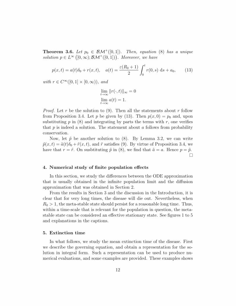
Figure 1: The first set of simulation compares the ODE solutions with theexpected values of the simulations obtained using the Gillespie algorithm(see Gillespie (1976)). From the results, it is apparent that even for pop-ulation that are not extremely large, the ODE approximation works wellprovided that a fair number of infected individuals already exist in the sys-tem. In these figures, we display the ODE solution for the infected fractioncompared against the average and mode across realisations obtained fromstochastic simulations using the Gillespie algorithm, for populations of sizesN = 50, 500. In all cases, the initial condition is I0 = 20% of the population.Figures (a) and (c) are for N = 500, while figures (b) and (d) were obtainedwith N = 50. In both cases, the the ODE is a good approximation of theexpected value, albeit with a larger variance in the case of N = 50. Themode across realisations is quite oscillatory, but it also is well approximatedby the ODE.

13

(a) (b)

(c)

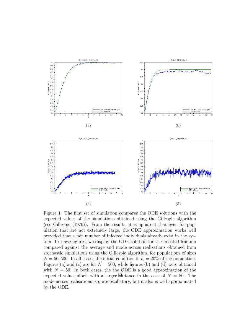
Figure 2: This second set depicts the solutions to the forward equation,where the development of a quasi-steady state for large times, and this canbe identified with quasi-stationary distribution. The initial condition was aDirac mass at 0.2N , with R0 = 2 for t ≥ 0, (a), and for t > 0.5, (b). In (a),one can clearly sees the trajectory that should be done by the mode and alsoby the expected value. In (b), the regular part is depicted in more detail.Notice that, for this particular initial condition, the Dirac measure at zerodid not develop significant mass up to the computed time. In (c), we showthe expected value of infected computing using the diffusive approximation,and compare with the ODE solution.

14

(a) (b)

(c) (d)

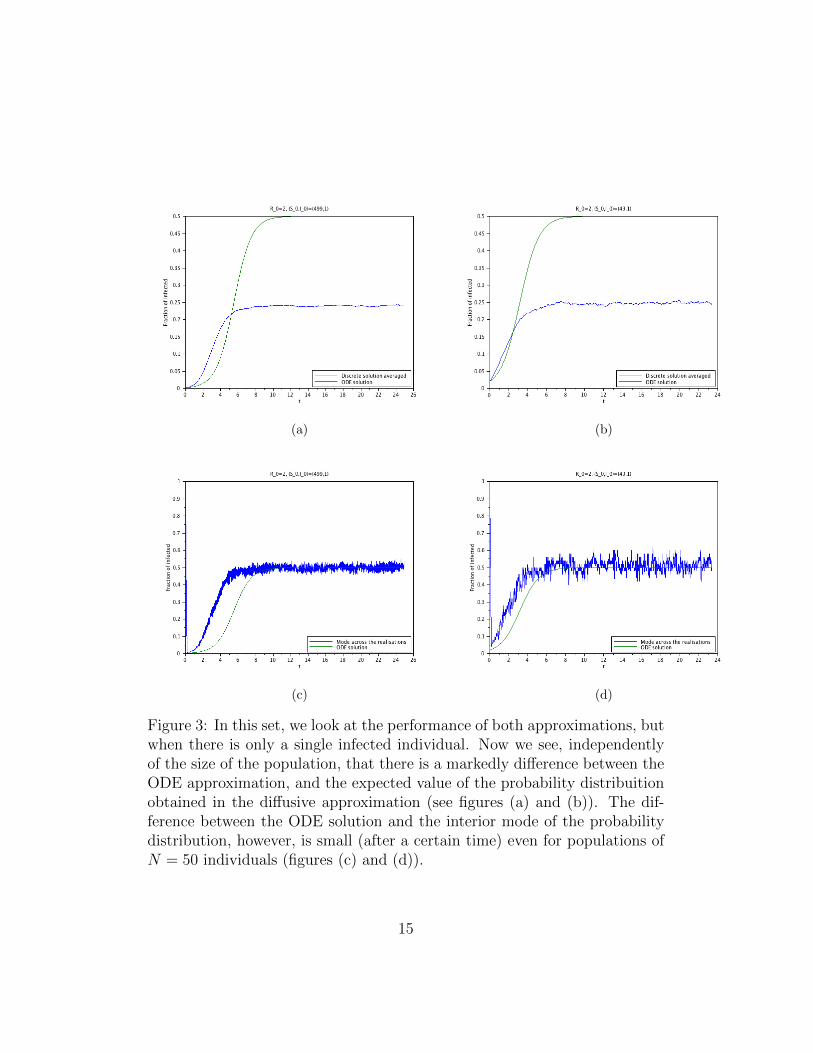
Figure 3: In this set, we look at the performance of both approximations, butwhen there is only a single infected individual. Now we see, independentlyof the size of the population, that there is a markedly difference between theODE approximation, and the expected value of the probability distribuitionobtained in the diffusive approximation (see figures (a) and (b)). The dif-ference between the ODE solution and the interior mode of the probabilitydistribution, however, is small (after a certain time) even for populations ofN = 50 individuals (figures (c) and (d)).

15

(a) (b)

(c) (d)

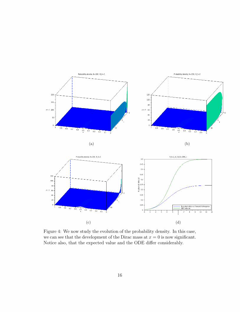
Figure 4: We now study the evolution of the probability density. In this case,we can see that the development of the Dirac mass at x = 0 is now significant.Notice also, that the expected value and the ODE differ considerably.

16

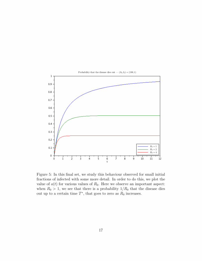
Figure 5: In this final set, we study this behaviour observed for small initialfractions of infected with some more detail. In order to do this, we plot thevalue of a(t) for various values of R0. Here we observe an important aspect:when R0 > 1, we see that there is a probability 1/R0 that the disease diesout up to a certain time T ∗, that goes to zero as R0 increases.

17

the boundary-layer nature of the solution when we have ε� 1, and thus weevaluate asymptotically this solution, for R0 > 1.

5.1. Formulation, integral representation and numerical examples

Let τε(x) denote the mean extinction time given that there are a fractionof x infected individuals at time zero.

Then, cf. Ewens (2004), we have that

ε

2τ ′′ε + Π(x)τ ′ε =

−1

ω(x), τε(0) = 0, and τ ′ε(1) = 0. (14)

In (14), we have that

ω(x) = x (R0(1− x) + 1)

and

Π(x) = 1− 2

R0(1− x) + 1.

If we take τ ′ε as the dependent variable, then (14) is a first order ODE for τ ′ε,satisfying τ ′ε(1) = 0.

Its solution is readily seen to be

τ ′ε(x) =2

ε

∫ 1

x

e2ε(s−x)

ω(s)

[R0(1− s) + 1

R0(1− x) + 1

] 4εR0

ds.

Hence

τε(x) =2

ε

∫ x

0

∫ 1

r

e2ε(s−r)

ω(s)

[R0(1− s) + 1

R0(1− r) + 1

] 4εR0

ds dr. (15)

Equation (15) can be rewritten as

τε(x) =2

ε(R0 + 1)

∫ x

0

∫ 1−r

0

eε−1φ(z,r)

[1

z + r+

1

x− (z + r)

]dz dr, (16)

where s = x+ z ,

x∗ = 1− 1

R0

, x = x∗ +2

R0

,

and

φ(z, r) = 4

[z

2+

1

R0

log

(1− z

x− r

)].

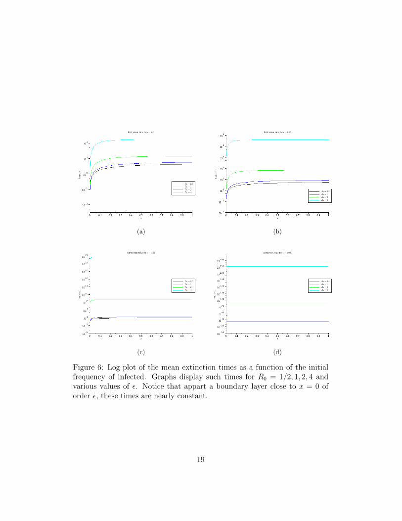
In Figure 6 we see a number of solutions of equation (15)—actually computedusing the representation given by (16). See caption for further discussion.

18

(a) (b)

(c) (d)

Figure 6: Log plot of the mean extinction times as a function of the initialfrequency of infected. Graphs display such times for R0 = 1/2, 1, 2, 4 andvarious values of ε. Notice that appart a boundary layer close to x = 0 oforder ε, these times are nearly constant.

19

5.2. Asymptotic evaluation

In order to evaluate (15) when ε � 1, we first need to evaluate τ ′ε(x).From (16), we have that:

τ ′ε(x) =2

ε(R0 + 1)

∫ 1−x

0

eε−1φ(z,x)

[1

x+ z− 1

x+ z − x

]dz. (17)

Before proceeding to evaluate (17) when ε� 1, we collect some useful factsabout φ.

1. φ(0, r) = 0 and, if R0 ≤ 1, we have φ(z, r) < 0, for z > 0, and r ≥ 0.

2. For R0 > 1, we have ∂zφ(0, r) > 0, for r < x∗. In this case, φ(·, r) hasa positive maximum at

z∗ = x∗ − r.This maximum will be relevant for the asymptotic evaluation providedthat r < x∗.

We shall study the case R0 > 1. The case R0 ≤ 1 is of less interest andwill be discussed elsewhere.

Notice that z∗ > 0, if x < x∗. Additionally, we compute

∂2zφ(x∗ − x, x) = −R0.

Thus, provided that 0 ≤ x ≤ x∗—and hence that 1− x ≥ z∗ ≥ 0—and usingthe steepest descent method, we obtain

τ ′ε(x)

= 2eε−1φ(x∗−x,x)f(x∗ − x)

x∗

(2π

R0

)1/2[N

((1− x∗)

(R0

ε

)1/2)−N

((x− x∗)

(R0

ε

)1/2)]

,

where N is the cumulative Normal distribution.For x > x∗, we have φ(z, x) < 0 for z ∈ [0, 1 − x], and hence that the

integrand is exponentially small, and can be neglected.Integrating the representation for τ ′ε and evaluating using Laplace’s method

yields

τε(x) = 2ex∗ε−1 f(x∗)

|f ′(x∗)|x∗

(2π

R0

)1/2 (1− e−|f

′(x∗)|x/ε). (18)

The asymptotic expression given by (18) suggest that, when R0 > 1, wecan have a very long persistence of the disease before it is eventually extinct.

20

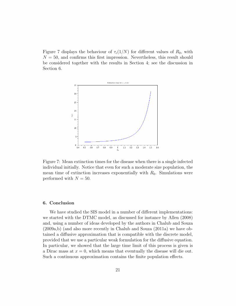
Figure 7 displays the behaviour of τε(1/N) for different values of R0, withN = 50, and confirms this first impression. Nevertheless, this result shouldbe considered together with the results in Section 4; see the discussion inSection 6.

Figure 7: Mean extinction times for the disease when there is a single infectedindividual initially. Notice that even for such a moderate size population, themean time of extinction increases exponentially with R0. Simulations wereperformed with N = 50.

6. Conclusion

We have studied the SIS model in a number of different implementations:we started with the DTMC model, as discussed for instance by Allen (2008)and, using a number of ideas developed by the authors in Chalub and Souza(2009a,b) (and also more recently in Chalub and Souza (2011a) we have ob-tained a diffusive approximation that is compatible with the discrete model,provided that we use a particular weak formulation for the diffusive equation.In particular, we showed that the large time limit of this process is given isa Dirac mass at x = 0, which means that eventually the disease will die out.Such a continuous approximation contains the finite population effects.

21

We then numerically studied both the DTMC model, the classical ODEmodel, and the diffusive approximation obtained here. The first observationis that the first and the third models displayed a very good agreement, ifthe initial condition was far from the absorbing state. This is was the caseeven for not very large populations. Nevertheless, given the simplicity ofthe model, such regime is not particularly interesting. We then studied thebehaviour for initial conditions with a single infected individual. Such aninitial condition is particularly important when trying to study the possibleonset of a disease that has just emerged. The results show the diffusive andstochastic model still with good agreement concerning the expected numberof cases, but this was not true for the ODE model. However, the ODE didrecover the mode of infected cases, after they stabilise.

We then proceed to use the fact that the PDE solution naturally de-composes as a Dirac measure supported at x = 0 with a time dependentintensity, and a regular part. The singular measure quantifies the likelinessof extinction of the disease at any given time, while the regular part stillapproximates the ODE behaviour with respect to the mode. In particular, acomprehensively study was made to understand the behaviour of these dif-ferent parts. The numerical studies then show that for larger values of R0 thedisease extinction probability increases up to 1/R0 at a certain characteristictime T ∗, that goes to zero as R0 increases. The regular part preserves thepart of the dynamics that is closer to the ODE approximation. Thus, thedisease has a probability of 1/R0 to disappear, and if that not occurs in acertain time T ∗, we shall have that the number of expected disease casesapproaches the one predicted by the ODE.

Also, using the corresponding backward equation, we could obtain themean extinction time (MET) and this was computed numerically in Section 5.When R0 > 1, such METs can have quite large values. We then derived anasymptotic approximation for the MET in this case, and we also computedits value when there is one single infected. Such METs displayed a very largeincrease as R0 increases.

Combining all these findings, we obtain that, when R0 > 1, there isa probability 1/R0 that a newly introduced disease will die out. If suchextinction does not occur until T ∗, it then goes to the inner equilibrium—which is well approximated by the ODE. Such an approximation can be seenas recovering the mode of the cases. Thus, the PDE model accounts correctlyfor both extreme regimes, and provides and explicit value of the probabilityof extinction. This might be of interest for public health questions, and we

22

hope to discuss this more thoroughly elsewhere.

Acknowledgments

FACCC: This work was partially supported by CMA/FCT/UNL, underthe project PEst-OE/MAT/UI0297/2011.

MOS: This work was partially supported by CNPq under the grant #309616/2009-3 and by the PRONEX Dengue initiative, under CNPq grant# 550030/2010-7.

References

Allen, L. J., 1994. Some discrete-time SI, SIR, and SIS epidemic models.Mathematical Biosciences 124 (1), 83 – 105.

Allen, L. J. S., 2008. An introduction to stochastic epidemic models. In:Mathematical epidemiology. Vol. 1945 of Lecture Notes in Math. Springer,Berlin, pp. 81–130.

Allen, L. J. S., Burgin, A. M., 2000. Comparison of deterministic and stochas-tic SIS and SIR models in discrete time. Math. Biosci. 163 (1), 1–33.

Anderson, R. M., May, R. M., 1995. Infectious diseases of humans: dynamicsand control, ¡1st ed. 1991, repr.¿ Edition. Oxford science publications.Oxford University Press, Oxford ¡etc.¿.

Auchmuty, G., 2005. Steklov eigenproblems and the representation of solu-tions of elliptic boundary value problems. Numerical Functional Analysisand Optimization 25 (3-4), 321–348.

Bailey, N. T. J., 1963. The simple stochastic epidemic: A complete solutionin terms of known functions. Biometrika 50 (3/4), pp. 235–240.

Bailey, N. T. J., 1975. The mathematical theory of infectious diseases and itsapplications, 2nd Edition. Hafner Press [Macmillan Publishing Co., Inc.]New York.

Chalub, F. A. C. C., Souza, M. O., 2009a. From discrete to continuous evo-lution models: A unifying approach to drift-diffusion and replicator dy-namics. Theor. Popul. Biol. 76 (4), 268–277.

23

Chalub, F. A. C. C., Souza, M. O., 2009b. A non-standard evolution problemarising in population genetics. Commun. Math. Sci. 7 (2), 489–502.

Chalub, F. A. C. C., Souza, M. O., 2011a. The frequency-dependent Wright-Fisher model: diffusive and non-diffusive approximations, preprint ArXiv.

Chalub, F. A. C. C., Souza, M. O., 2011b. The SIR epidemic model from aPDE point of view. Math. Comput. Modelling 53 (7-8), 1568–1574.

Evans, L. C., 2010. Partial Differential Equations, 2nd Edition. Vol. 19 ofGraduate Studies in Mathematics. American Mathematical Society, Prov-idence, RI.

Ewens, W. J., 2004. Mathematical population genetics, 2nd Edition. Vol. v.27. Springer, New York.

Gillespie, D. T., 1976. A general method for numerically simulating thestochastic time evolution of coupled chemical reactions. Journal of Com-putational Physics 22 (4), 403 – 434.

Lieberman, G., 1996. Second Order Parabolic Differential Equations. WorldScientific.URL http://books.google.com.br/books?id=s9Guiwylm3cC

McKane, A. J., Newman, T. J., Oct 2004. Stochastic models in populationbiology and their deterministic analogs. Phys. Rev. E 70, 041902.

Rass, L., Radcliffe, J., 2003. Spatial deterministic epidemics. Vol. 102 ofMathematical Surveys and Monographs. American Mathematical Society,Providence, RI.

Taylor, M. E., 1996. Partial Differential Equations. I. Vol. 115 of AppliedMathematical Sciences. Springer-Verlag, New York, basic theory.

Van Segbroeck, S., Santos, F. C., Pacheco, J. M., 2010. Adaptive contact net-works change effective disease infectiousness and dynamics. PLoS ComputBiol 6 (8).

24