Determination of hot- and cold-rolling texture of steels: A combined Bayesian Neural

Network model

C. Capdevila, I. Toda, F.G. Caballero, C. Garcia-Mateo and C. Garcia de Andres

Materalia Research Group, Department of Physical Metallurgy, Centro Nacional de Investigaciones

Metalúrgicas (CENIM), consejo Superior de Investigaciones Científicas (CSIC), Avda. Gregorio del Amo, 8. E-

28040 Madrid, Spain

Abstract

The work reported in this paper outlines the use of a combined artificial neural network model capable of fast

online prediction of textures in low and extra low carbon steels. We approach the problem by a Bayesian

framework neural network model that take into account as input to the model the influence of 23 parameters

describing chemical composition, and thermomechanical processes such as austenite and ferrite rolling, coiling,

cold working and subsequent annealing involved on the production route of low and extra low carbon steels.

The output of the model is in the form of fiber texture data. The predictions of the network provide an

excellent match to the experimentally measured data. The results presented in this paper demonstrate that

this model can help on optimizing the normal anisotropy (rm) of steel products.

Keywords: Artificial Neural Network; Texture prediction; Anisotropy; Hot Rolling; Cold rolling; Steel

Introduction

In recent years there has been a steady increase of interest from the automotive industry in isotropic steel

product; i.e. steel products with a minimum of variation of mechanical properties, most noticeably drawability,

in the plane of the sheet. Therefore, corresponding to the ever increasing demands of the sheet metal forming

industry, future generations of drawable steel grades will need to ensure a well-balanced equilibrium between

drawability on the one hand and drawing anisotropy on the other hand.

Great demands are placed on the quality of deep drawing steels with regard to their surface and mechanical

properties. The knowledge of the microstructural and textural evolution in the individual process stages is of

highest importance to improve sheet quality in terms of its deep-drawing properties. In the past the derivation

of models for microstructural and textural evolution was carried out on the basis of the results of laboratory

tests using the reversing rolling technique. This applies in particular to the rolling experiments which can be

performed at low rolling speeds only, e.g. approximately 1 ms-1 and inter pass times > 5 seconds.

Nevertheless, the continuously increasing requirements on the quality of flat products demand the further

development of both materials and their production technologies. Such development can be achieved in

modern continuous hot strip mills which operate with rolling speeds of up to 20 ms-1 and inter pass times of 0.1

s. From this follows, that differences in microstructure and properties existed between strips rolled in the

laboratory and in practice, which reveals that laboratory plants and even pilot mills often cannot accurately

simulate production conditions.

To close this gap, in this paper it was decided to employ an entirely new tool, patterned to human brain: the

‘artificial neural networks’. Such networks ‘learn’ from the massive volume of incoming data and the

relationships involved and gain experience from systematic observation of recurring events. This makes them

capable of supporting traditional mathematical models or replacing them entirely. Their learning ability also

enables neural networks to adapt continuously to changing process states. This paper illustrates the use of

such modelling technique in the prediction of texture for low-carbon (LC) and extra low carbon (ELC) deep

drawing steel qualities as a function of chemistry and thermomechanical processing parameters. The drawing

properties of the steel are essentially determined by the texture of the finished product. The model is then

used in the prediction of the normal anisotropy ratio, or the rm value, for LC and ELC steel. The rm value

evaluates the drawability of a sheet material, i.e. its capacity to achieve a high degree of plastic flow in the

plane of the sheet while offering sufficient resistance to flow in the thickness direction. On this basis, the work

reported here provides an example of how neural network modelling could be incorporated into the

optimization process of steel sheets and how the rolling processing parameters affects the texture of such

steels that satisfy the increasing drawability of advanced steel for automotive applications.

Build of the model

The drawing properties of the steel are essentially determined by the texture of the finished product [1]. Figure

1 shows the 2 = 45deg sections of the ODF, because this section contains all the important rolling and

recrystallisation components of a BCC material. The texture components depicted in Fig. 1 can be used as a key

to read the texture results obtained by the model. In this figure it can be seen that the dominant components

mainly concentrate along two fibers: α-fiber (RD||<110>), with main texture components within the range

{001}<110> (ϕ1=0, =0, ϕ2=45) to {111}<110> (ϕ1=0, =55, ϕ2=45), and the γ-fiber (ND||<111>), where

RD is the rolling direction and ND is the direction parallel to the sheet normal. It is commonly known that for a

BCC material the y-fibre <111>||ND texture is the desired texture type to obtain the highest drawability. In

consequence, texture control in drawing steel grades consistently aims to develop the highest possible

intensity along the y-fibre.

The texture strength has been modelled by determining the - and - fibers intensities (f(g)). The -fiber

intensity has been calculated for 0<<90 in steps of =5. Each step corresponds to an independent neural

network model. On the other hand, the -fiber has been calculated for 60<1<90 in steps of 1=10, with

independent models for each step. Therefore, 19 different models have been developed to characterise the -

fiber, and 4 models to characterize the -fiber.

In this sense, the focus of this work was the investigation of the influence of rolling parameters on the - and -

fibers of hot strip, and derived cold strip, from ultra-low carbon (ULC), interstitial free (IF), low-carbon (LC),

high-strength low-alloyed (HSLA), and extra-low carbon (ELC) steel grades. Figure 2 shows the product flow and

the major characteristics of the hot and cold strip mill line. The following parameters were varied to investigate

their effects on strip properties: roughing temperature and reduction, reheating temperature, finishing

temperature and reduction, rolling speed, cooling conditions, coil temperature, and rolls with roll gap

lubrication.

A second aim of this paper is to clarify the impact of the hot strip state on the properties of cold strip. In this

sense, parameters such as cold rolling reduction and annealing temperature were systematically analysed and

incorporated in the dataset. Likewise, special attention has been paid to the influence of hot-rolling on

subsequent cold-rolled microstructure. The proposed model allows a more deep understanding of the

influence of each parameter of the rolling stand (hot and cold rolling) on the final microstructure of deep

drawable steels. Furthermore, this model allows a systematic development of new materials with regard to

deep drawing properties depending on the deformation conditions.

Database

The models that constitute the - and -fibers require a complete description of the chemical composition and

processing parameters. A literature survey [2-9] allows us to collect 240 individual cases where detailed

chemical composition, hot-rolling processing parameters, coiling temperature, cold reduction and annealing

temperature values were reported for each of the 18 individual models which form the -fiber, and the 4

individual models that form the -fiber. The hot-rolling data collected correspond to those obtained from pilot

mill. The pilot mill comprises four rolling stands so arranged in one line that roughing is possible with one

reversing two-high stand, followed by continuous finishing with all four stands (reversing two-high plus three

continuous two-high stands). Samples are heated in an inductor allowing fast heating to 1350°C. All stands are

equipped with roll gap lubrication, and interpass times can be varied by modification of the rolling speeds and

the distances between stands. The hot-rolled samples are then cold-rolled and continuously annealed in a

radiation furnace simulator.

The variables considered are the following: chemical composition in weight pct (carbon (C), manganese (Mn),

silicon (Si), aluminium (Al), chromium (Cr), nitrogen (N), niobium (Nb) and titanium (Ti)), reheating temperature

(SRT), roughing stage (temperature (RT), speed (RS), passes (nR) and reduction (RRED)), finishing stage

(temperature (FT), speed (FS), passes (nF) and reduction (FRED)), the use of lubricant during rolling (LUB:

without = 0; and lubricant = 1), coiling temperature (CT), cold-rolling reduction (CRED), and finally annealing

temperature (AT)). Table 1 shows the list of 23 input variables used for the - and -fibers analysis, and Table 2

lists the output variables considered.

Brief description neural network

The aim is to be able to estimate f(g) evolution with for -fiber and with 1 for -fiber as a function of the

variables listed in Table 1. In the present case, the network was trained using a randomly chosen of 130

examples from a total of 240 available; the remaining 110 examples were used as new experiments to test the

trained network. Linear functions of the inputs xj are operated by a hyperbolic tangent transfer function

(1)

)1(

i

j

j)1(

iji xwtanhh

So that each input contributes to every hidden unit. The bias is designated i(1) and is analogous to the constant

that appears in linear regression. The strength of the transfer function is in each case determined by the weight

wij(1). The transfer to the output y is linear

(2)

This specification of the network structure, together with the set of weights, is a complete description of the

formula relating the inputs to the output. The weights were determined by training the network and the details

are described by MacKay [10-11]. The training involves a minimization of the regularized sum of squared errors.

The term v was the framework estimation of the noise level of the data. Figure 3 shows, as an example, the

inferred noise level of = 45 model. It is clear from the figure that the inferred noise level decreases

monotonically as the number of hidden units increase. Table 2 list the v values obtained for each model.

However, the complexity of the model also increases with the number of hidden units. To find out the

optimum number of hidden units of the model the following procedure was used. The experimental data were

partitioned equally and randomly into a test dataset and a training dataset. Only the latter was used to train

the model, whose ability to generalist was examined by checking its performance on the unseen test data. The

test error (Ten) is a reflection of the ability of the model to predict in the test data:

(3)

where yn is the set of predictions made by the model and tn is the set of target (experimental) values.

A high degree of complexity may not be justified, and in an extreme case, the model may in a meaningless way

attempt to fit the noise in the experimental data. MacKay [12-13] has made a detailed study of this problem,

and defined a quantity (the ‘evidence’) which comments on the probability of a model. In circumstances where

two models give similar results for the known data, the more probable model would be predicted to be that

which is simpler; this simple model would have a higher value of evidence. The evidence framework was used

to control v. The number of hidden units was set by examining performance on test data. A combination of

Bayesian and pragmatic statistical techniques were therefore used to control the complexity of the model [14].

For the particular case of = 45 model shown in Figure 3, it could be concluded that a large number of hidden

i

)2(i

)2(i hwy

n

2nnen ty5.0T

units did not give significantly lower values of v; indeed, eleven hidden units were found to give a reasonable

level of complexity to represent the variations of f(g) as a function of the input variables of Table 1.

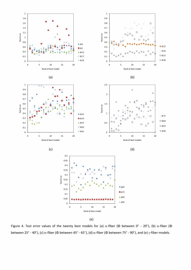
On the other hand, it is possible that a committee of models can make a more reliable prediction than an

individual model. The best models were ranked using the values of their test errors (equation (3)) as Fig. 4(a)-

(d) and Fig. 4(e) present, for the respective -fiber and -fiber. Committee of models could then be formed by

combining the prediction of the best L models, where L = l, 2,... The size of the committee is therefore given by

the value of L.

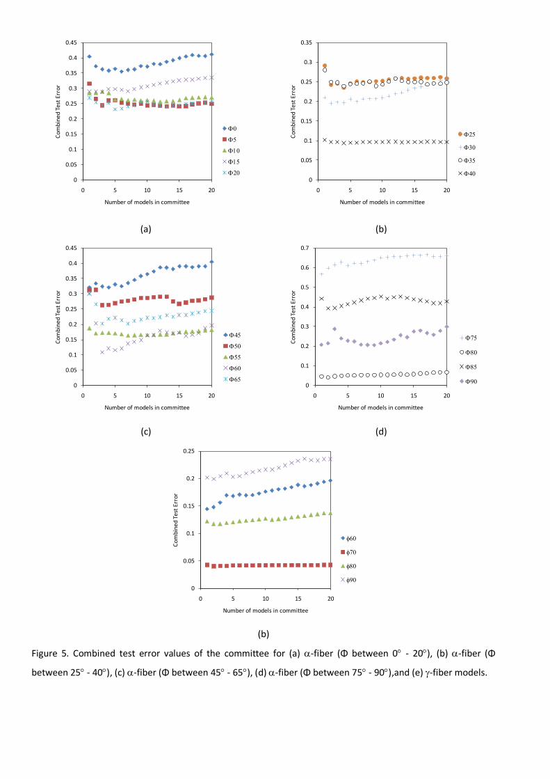
The combined test error of the predictions made by a committee of L models, ranked 1 ,2...q...L, each with n

lines of test data, is calculated in a similar manner to the test error of a single model:

(4)

where is the set of predictions made by the model and tn is the set of target (experimental) values. As

Figure 5 suggests the combined test error goes through a minimum for the committee made up of certain

number of models as it is listed in Table 3. However, there some exceptions such as the one for = 75 and =

60 models where the build of a committee does not reduced the test error. In such cases, the best model is

considered only. From a comparison between results presented in Figures 4 and 5 it is clear a reduction in test

error and hence improved predictions by using the committee of models approach instead of the best model

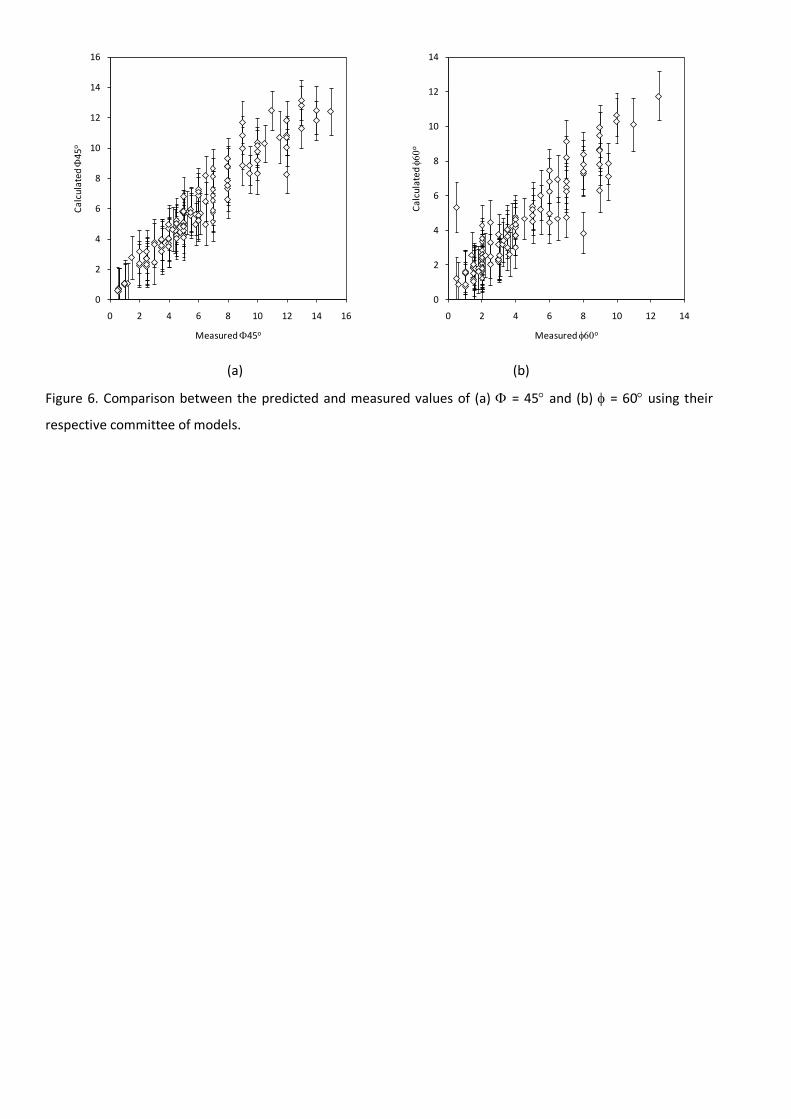
alone. Comparison between the predicted and measured values of = 45 and = 60, as an example, for the

training and test data is shown in Fig. 6 for the best committee of each fiber component.

Nevertheless, the practice of using a best-fit function does not adequately describe the uncertainties in regions

of the input space where data are spare or noisy. MacKay [12,13] has developed a particularly useful treatment

of neural networks in a Bayesian framework, which allows the calculation of error bars representing the

uncertainty in the fitting parameters. The method recognizes that there are many functions which can be fitted

or extrapolated into uncertain regions of the input space, without unduly compromising the fit in adjacent

regions which are rich in accurate data. Instead of calculating a unique set of weights, a probability distribution

of sets of weights is used to define the fitting uncertainty. The error bars therefore become larger when data

are spare or locally noisy.

q

)q(nn

n

2

nnen

yL

1y

ty5.0T

)q(ny

Figures 7 and 8 illustrate the significance (w) of each of the input variables, as perceived by the neural

network, in influencing the components of - and -fibers, respectively. The variables analysed are organized in

three groups, i.e. Group 1: hot rolling, Group 2: chemical composition and Group 3: cold rolling and annealing

(see Table 1). The value of w is normalized to 100, i.e. the value of w for a specific variable indicates the

degree of influence in percentage. The metallurgical significance of the results predicted by the models is

discussed below, but a first approximation of the influence of each one of the variables studied could be drawn

from a close observation of Figs. 7 and 8.

As general comment for the 19 models of -fiber components, and the 4 models of -fiber models, it is clear

that the annealing temperature (AT) after cold rolling, together with cold-rolling reduction (CRED), clearly have

a large intrinsic effect on -fiber components, and in a minor scale on -fiber components. In terms of hot

rolling processing parameters the finishing stage has a significantly larger influence that the roughing stage.

Particularly, the slab reheating temperature (SRT) and the finishing temperature (FT) significantly affect the

intensity of the -fiber components for the case of 0 to components. A relative low influence of those

parameters is observer for the remaining components of -fiber. It is also worth mentioning the lack of

influence of a priori important variables such as finishing reduction (FRED), speed of rolling (FS) and the

number of steps involved in the finishing process (nF).

On the other hand, finishing and roughing temperatures has a large influence on the components of -fiber,

which is of technological importance since the intensity of such fiber is closely related with the deep drawing

properties of the steels as it has been thoroughly reported in literature in the last decade.

Special attention to the role of chemical composition on the f(g) values of - and -fiber components has been

paid. The chemical composition is not very relevant for the development of -fiber components (with the

exception of 70 component). However, it is important to highlight the spectacular relevance of microalloying

elements such as Nb and Ti have on the intensity of -fiber components. This is consistent with the well

reported influence of these microalloying elements on tiding up the interstitial elements such as C and N,

which have a negative influence on the development of good deep drawability properties. This broad idea is

consistent with the high influence of C content in -fiber components, is it is seen in Fig. 8.

It is surprising the high influence that lubricant (LUB) has on 0 component of -fiber, which could be related

with the role of shear friction during rolling on the development of such component as it has been reported

[15]. On the other hand, this parameter has a rather negligible influence on the remaining - and -fiber

components.

Applications of the model: Evolution of hot-rolling texture in IF steels

The effect of rolling parameters such as SRT, FS and FT on a IF steel is reported in this section (see Table 4 for

chemical composition). It has been considered two situations: IF steel hot rolled in the austenitic (FT = 930 C)

as well as in the upper (FT = 800 C) and lower ferritic region (FT = 650 C). For the ferritic rolling a high and a

low reheating temperature of 1250 °C respective 1050 °C have been investigated. Two different rolling speeds

in the finishing mill have been considered (0.5 and 7 m s-1).

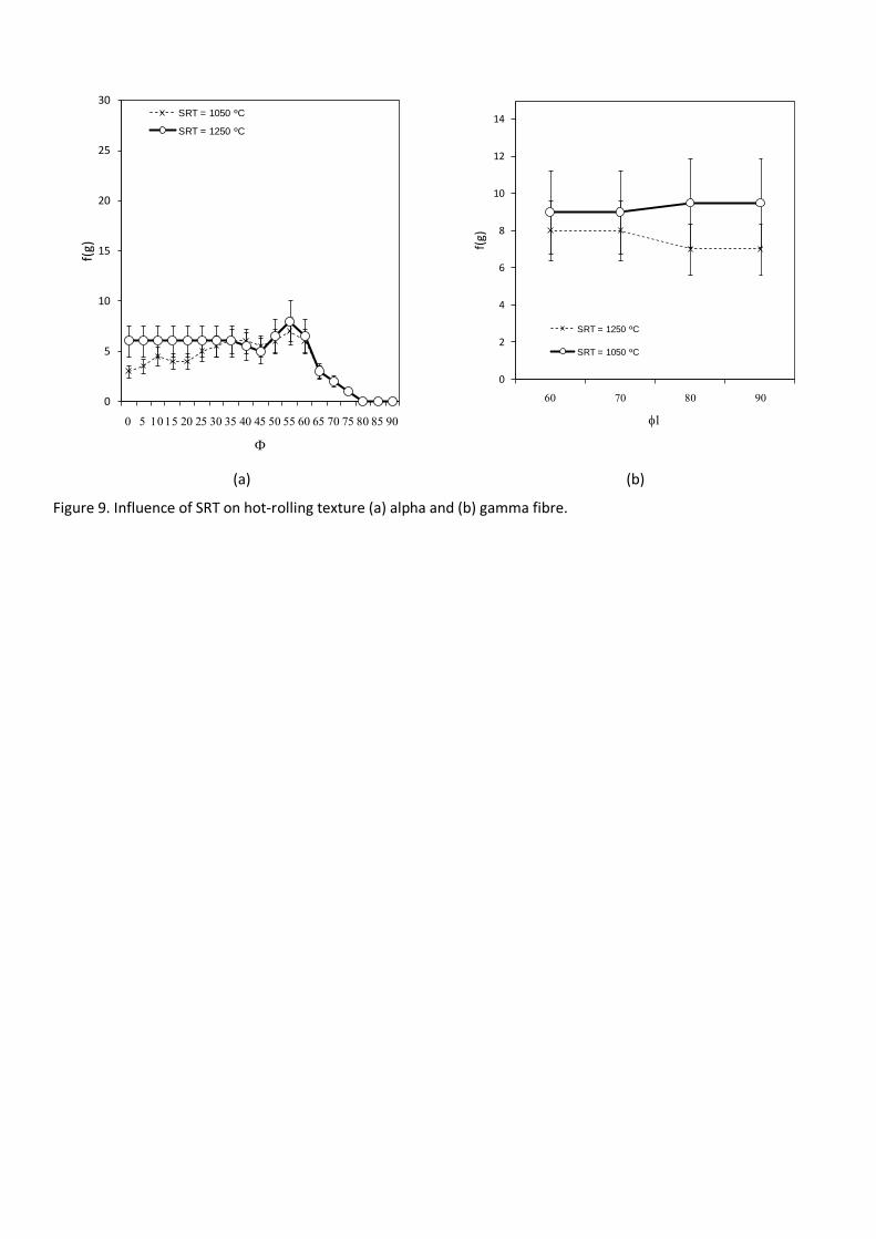
Figure 9 shows the evolution of both alpha and gamma fibres for the two SRT selected. The FT value considered

in calculations is 930 C and FS = 0.5 m s-1. The remaining rolling parameters considered are listed in Table 4. It

is clear from the results presented that simulations are consistent with the typical low intensities on their alpha

and gamma fibre expected after hot rolling processing. It could be concluded that there is not significant

influence of SRT on hot-rolling texture.

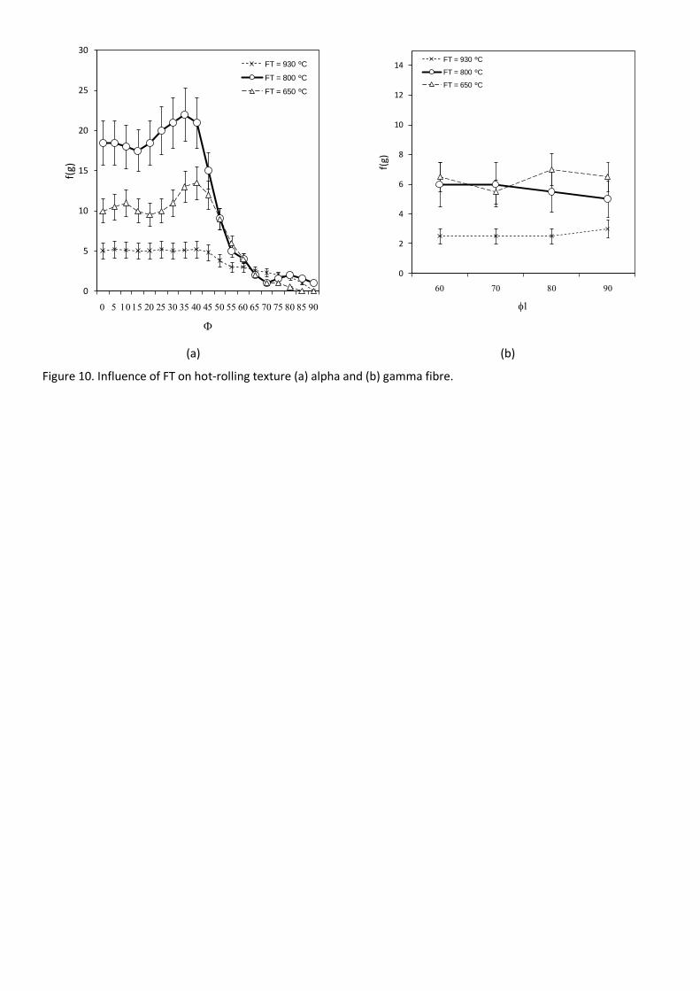
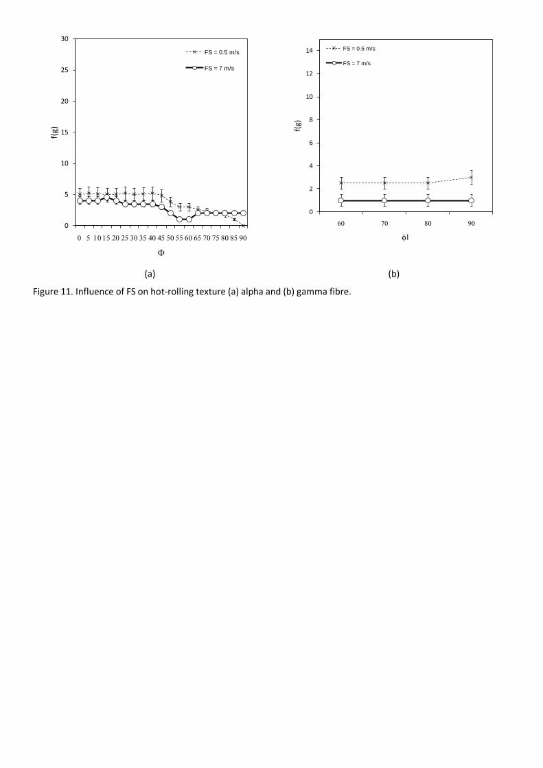
On the other hand, Figure 10 presents the results for the influence of FT on hot-rolling texture. It has been

selected three different temperatures. A FT of 930 C which indicates an austenitic rolling and subsequent air-

cooling to room temperature, and FT values of 800 and 650 C for the upper and lower ferrite region with the

higher reheating temperature of 1250°C (see Table 4 for remaining processing parameters). Compared with

austenitic rolling the intensities are significantly higher both for the alpha and the gamma fibre. Significant

differences of the intensities can be observed especially for the alpha fibre but also for the gamma fibre with FT

in the ferrite-region. However, they could not be linked to an influence of rolling parameters such as SRT, RT

and LUB. The attempt to link the differences to the roll speed fails. Figure 11 shows the differences in both

alpha and gamma fibres with FS for a FT = 800 C (see Table 4 for remaining parameters).

Applications of the model: Effect of chemical composition and processing parameters on the normal

anisotropy index (rm) in DDQ steels

On deep drawability quality (DDQ) steel, particular attention to {111}<uvw> orientation should be paid [16-17].

It has been demonstrated that high rm values are displayed by materials which have a high proportion of grains

oriented with their {111} planes parallel to the sheet plane, i.e. by materials which possess a strong {111}} type

texture (or -fibre texture). Other texture components, such as the {001}, have been found to be detrimental to

the drawability and, in this sense, and according with the work reported by Daniel and Jonas [18], the most

desired texture components to obtain good drawability properties are {111}<110> and {111}<112>, and the

most undesired ones will be {110}<001> and {001}<110>. In practice, the intensity ratio of the above two

components, I(111)/I(100), is found to be linearly related to rm as it was determined by Held [19]. This author

measured the evolution of rm with the - and -fibres intensities ratio, and concluded that there is a linear

relationship expressed by

(5)

Therefore, the influence of different processing parameters (and chemical composition) on rm can be evaluated

through the I(111)/I(100) ratio by means of the neural network model developed in this work. Table 5 lists the

conditions considered in calculations. More precisely, it has been considered two alternative processing routes

denoted as ‘hot rolling’ and ‘cold rolling and annealing’. The former consist on processing the material as it is

done in a traditional hot-rolling mill, meanwhile two additional stages (cold rolling deformation with a

thickness reduction of 80%) and annealing temperature are added to the latter one. Those varying parameters

are indicated.

Effect of chemical composition

Figure 12 shows the evolution of rm for carbon content ranging from 0.002 wt% to 0.02 wt%. Constant values of

Nb and Ti contents (i.e, [Nb] = 0.029 wt% [Ti] = 0.037 wt%) have been considered. Regarding the processing

parameter, fixed values of finishing rolling temperature (FT = 930 C), coiling temperature (CT = 700 C), and

annealing temperature (AT = 750 C) have been used in calculations. The first conclusion that can be drawn

from this figure is the significantly higher rm value for a cold-rolled and annealed material as compared with a

hot-rolled one, which is a consequence of the dramatic texture differences between hot-rolled and cold-rolled

and annealed steels. The recrystallisation of austenite during hot rolling (with a FT = 930 C) is unimpeded in

and is sufficiently rapid to be essentially completed before the transformation to ferrite. This leads to an

absence of texture components in the ferrite, since austenite did not contain any rolling components before

transformation [20]. However, the cold rolling process induces a stored energy in the material that it is

released during subsequent annealing treatment leading to the formation of deformation-free grains

(recrystallization). On the basis of stored-energy considerations, the final texture should be dominated by

nuclei which form soonest and which are most numerous. On this basis, the {111} components and a spread of

random orientation may be expected, together with a small {110} component, in the cold-rolled and annealed

steel as compared with hot-rolled one. This leads to a stronger I(111)/I(100) ration and hence to a bigger rm

value.

Figure 12 also shows a decrease of rm as C-content increases for cold-rolled and annealed steel. This result is

fully consistent with work reported by Fukuda [21] where showed that rm increased progressively with

decrease in the amount of carbon. These effects have subsequently been corroborated by other workers [22]

and confirm the broad idea that high levels of carbon were undesirable in deep drawing quality steels, which

can probably be attributed to unfavorable annealing texture components nucleated around the harder second

-phase pearlite islands.

Figures 13 and 14 show the influence of Ti and Nb additions on rm values. The C content in both calculation is

kept constant with a value of [C] = 0.002 wt%, FT = 930 C, CT = 700 C, and AT = 750 C. It is clear that in both

cases the annealed microstructure presents a significant increase in rm value as the content of both Ti and Nb

increases. On the other hand, there is an opposite effect in the hot-rolled microstructure. Meanwhile an

increase in Ti content raises the value of rm, an equivalent increase in Nb content induce a drop in rm value.

These results are consistent with the work reported by Hook and co-workers [23-24], where it was concluded

that the austenite in the Nb steel is essentially pancaked (unrecrystallised), while the austenite is partially

recrystallised in the Ti steel. The retardation of austenite recrystallisation in the Nb steel during hot rolling is

attributable to two complementary factors: (a) the presence of solute Nb in the austenite, and (b) the

precipitation of Nb carbonitrides in the matrix. Finally, as it is well know [25,26], the unrecrystallized austenite

leads to a finer microstructure after austenite-to-ferrite transformation, and the finer the microstructure the

lower the I(111)/I(100) ratio [27], which can explain the decrease of rm value in Nb-bearing steels as compare

with Ti steels after the hot rolled stage.

Regarding the cold rolled and annealed results, it is clear that both Ti and Nb increase the rm value. This is

because of the very effective role of both Nb and Ti on tiding up the interstitials in the steels. If the carbon in

solid solution is tied up by Nb or Ti, an extensive recovery goes on the gamma grains and the local areas of high

concentration of deformation energy quickly become potential nuclei of {111} orientation. This strengthens the

-fiber and hence the I(111)/I(100) ratio increases. However, if the amount of carbon is high (not enough Ti

and/or Nb in solid solution), the recovery is sluggish due to C-Mn dipoles immobilizing dislocations. In such a

case the grains of lower concentration of deformation energy grow at expense of the highly deformed {111}

grains through a process of stress induced boundary migration. Therefore, the I(111)/I(100) ratio is weaken,

and hence rm decreases.

Effect of processing parameters

The values of C, Ti and Nb considered in calculation are, respectively, [C] = 0.002 wt%, [Ti] = 0.037 wt% and

[Nb] = 0.029 wt%. A value of coiling temperature of CT=700 Co has been considered in predictions. Figure 15

shows the influence of FT on rm value for both hot-rolled and cold-rolled and annealed materials. It is worth

mentioning that the FT values considered here include both the austenitic and ferritic rolling. The observed

increase of rm value as FT deceases is related with the fact that at low FT values the steel is fully transformed to

ferrite. The situation is therefore comparable with warm ferritic rolling procedure where rolling takes place in a

ferritic stage. Thus, the formation of shear bands occurs which promotes the formation of dynamically

recovered grains of {111} orientation enhancing the development of a strong -fiber texture [28]. This is

consistent with the increase in rm value observed.

Regarding the evolution of cold-rolled and annealed material, a more complex behavior is observed. There is a

maximum for a FT value of 850 C which is the lowest FT to ensure a complete austenitic rolling. In the

austenitic rolling regime, lower FT induces an unrecrystallized austenite which promotes the formation of a

very fine ferrite grains during subsequent austenite-to-ferrite transformation. During annealing after cold-

rolling, the {111} grains nucleate in the grain boundaries of deformed ferrite grains. Therefore, the finer the

deformed ferrite grain, the more abundant {111} nucleation events. Thus, the -fibre strengthens with the

concomitant increase in rm value. This can explain the increase of rm when FT is lowered in the austenitic rolling

regime.

However, as it was reported by Jeong [29], ferrite grain after hot-rolling markedly coarsens with a decrease in

the FT. When the FT is lower than Ar3, the grain structure just after hot-rolling in two phase region of ferrite

and austenite consists of the deformed ferrite and deformed austenite grains. The deformed austenite grains

immediately transform to strain-free ferrite grains which grow to the surrounding deformed ferrite grains

during cooling and coiling simulation at 700 °C, leading to the coarse-grained structure. The microstructural

change with the finishing temperature in hot-rolling is partially responsible for the change in the textural

evolution during the subsequent cold-rolling and annealing, since cold-rolled microstructure is still reflecting

the coarse structure of the hot-rolled steel. Therefore, the formation of {111} grains at grain boundaries of

deformed ferrite grains is overcome by a stronger development of the {100} <011> orientation in the annealed

sheet, leading to a subsequent decrease in rm values.

Figure 16 shows the effect of CT on rm value. Regarding the hot rolled material, the effect of CT is negligible.

Only a slight increase of rm is observed at low CT values. However, a clear influence on cold-rolled and annealed

material is observed. This behavior is consistent with experimental observations [30-31], where it was reported

that final textures are improved by coiling the hot band at high temperature, i.e. above about 700°C. With high-

temperature coiling, the carbide precipitation occurs during very slow cooling of the coiling, and the carbide

constituents become coarser and more widely dispersed. Therefore, the ferrite becomes almost completely

pure, since any residual carbon diffuses to the cementite particles and precipitates out [32-33]. If these

carbides are widely spaced and if the steel is heated rapidly after cold rolling, it is possible for recrystallization

of the ferrite to take place before significant re -solution of the carbon can occur. The resulting texture contains

a strong {111} component, and hence a high rm value.

Figure 17(a) shows the evolution of rm value with annealing temperature after cold-rolling (80% reduction in

thickness). It could be concluded from the figure that the higher the annealing temperature the higher the rm

value. This is consistent with the work reported by Petite et al. [27] which demonstrated that there is a linear

relationship between the recrystallized grain size and the rm value. Therefore, the higher the annealing

temperature, the coarser the grain grows and hence higher values of rm are achieved.

On the other hand, the carbide dispersion formed during coiling is very important since coarse carbides are

very effective on on wiping out carbon from ferrite matrix, but fine dispersion of carbide particles produced by

low-temperature coiling can release carbon into the matrix during cold rolling by a kind of mechanical-

dissolution process. According to this view, the dissolved carbon causes dynamic strain aging and leads to

inhomogeneous (constrained) deformation in the form of shear bands, which, on subsequent annealing, induce

nucleation of unfavorably oriented grains [34]. The fact that carbon can operate in two different ways, i.e.

during deformation and during annealing, is highly confusing. In order to clarify this combined effect, Fig. 18

shows the combined influence of CT and AT on rm values. It is clear from the figure that the best result in terms

of high rm value is obtained at high-CT combined with high-AT values, where the coarser carbides are formed

and the fast recrystallization will avoid the nucleation of some unfavorable recrystallized grains around the

coarser carbides [35-36].

Conclusions

A combined neural network under a Bayesian framework has been developed to predict the texture evolution

in low and extra low carbon steels. This model consists in the combination of 23 individual neural network

models to deal with the evolution of -fibre and -fibre by varying 23 input parameters describing chemical

composition, and thermomechanical processes such as austenite and ferrite rolling, coiling, cold working and

subsequent annealing involved on the production route of low and extra low carbon steels. The predictions of

the network within the bounds of the training data set show a good match to the measured values, allowing us

to conclude that this combined model is a powerful tool for fast online prediction of textures in an engineering

environment.

The combined neural network model created has been applied to predict the evolution of anisotropy index (rm)

in DDQ steels with varying chemical composition (C, Ti and Nb content) and processing parameters such as

finishing rolling temperature (FT), coiling temperature (CT), and annealing temperature (AT) after cold-rolling.

The results obtained allow us to conclude that cold-rolling and annealing processing present a substantially

higher rm value as compare with hot rolling processing.

The model presented in this paper has been revealed very useful on predicting the influence that C, Ti and Nb

in solid solution exert on rm value. Higher carbon levels in solid solution are associated with weaker textures,

reducing the rm value. On the other hand, the Ti and Nb content substantially increase the rm value.

The perception of the model to varying values of FT, CT and AT is consistent with measurements reported in

literature. Particular attention to the effect of CT and AT has been paid. It has been demonstrated that rm value

is very sensitive to both parameters. The low-CT temperature allows higher amounts of carbon to remain in

solid solution in ferrite, and then has a detrimental effect on rm values. Meanwhile high CT leads to sharper

{111} fibre and improved rm values.

Acknowledgements

The authors acknowledge financial support from the Spanish Ministerio de Ciencia e Innovación through the

Plan Nacional 2009 (ENE2009 13766-C04-01). The authors are also grateful to Neuromat Ltd. for the provision

of the neural network software used in this work.

References

[1] B. Hutchinson: Ironmaking and Steelmaking, 2001, 28, 145-151.

[2] R. Kawalla, W. Jungnickel, H.P. Schmitz, G. Paul, A. De Paepe and W.M. von Haaften: ‘Effect of hot and cold

rolling technology on textures and plastic anisotropy of flat products’, ECSC Report, European Commission,

Luxembourg, 2007.

[3] L. Kestens, I. Gutierrez, J. L. Bocos, J. Zaitegui, V. Cascioli, P E. Di Nunzio and R. Groterlinden: ‘Texture

control in cold-rolled steel sheets for an optimised arlisotropy’, ECSC Report, European Commission,

Luxembourg, 2002.

[4] T. Iung, G. Lannoo, C. Garcia de Andres and I. Salvatori: ‘Metallurgical aspects of the compact reheating

treatment of hot-rolled strips before coiling’, ECSC Report, European Commission, Luxembourg, 2007.

[5] C. Capdevila, T. De Cock, C. Garcia-Mateo, F. G. Caballero and C. G. de Andres: Mater. Sci. Forum, 2005, 500-

501, 803-810.

[6] C. Capdevila, J. P. Ferrer, F. G. Caballero and C. G. De Andres: Metall. Mater. Transactions A, 2006, 37, 2059-

2068.

[7]F. G. Caballero, C. Capdevila and C. de Andres: Mat. Sci. Technol., 2001, 17, 1114-1118.

[8] C. Capdevila, C. Garcia-Mateo, F. G. Caballero and C. G. de Andres: Mater. Sci. Technol., 2006, 22, 1163-

1170.

[9] J. P. Ferrer, T. De Cock, C. Capdevila, F. G. Caballero and C. G. de Andres: Acta Mater., 2007, 55, 2075-2083.

[10] D.J.C. MaKay: Neural Comput., 1992, 4, 698-705.

[11] D.J.C. MaKay: Darwin college J, 1993, 3, 81-93.

[12] D.J.C. MaKay: Neural Comput., 1992, 4, 415-422.

[13] D.J.C. MaKay: Neural Comput. 1992, 4, 448-460.

[14] H.K.D.H. Bhadeshia: ISIJ Int., 1999, 39, 965-979.

[15] Y. Hayakawa and J. A. Szpunar: Acta Mater., 1997, 45, 4713-4720.

[16] W. B. Hutchinson: Int. Metals Rev., 1984, 29, 25-42.

[17] R. K. Ray, J. J. Jonas and R. E. Hook: Int. Mater. Rev., 1994, 39, 129-172.

[18] D. Daniel and J. J. Jonas: Metall. Trans. A., 1990, 21, 331-342.

[19]. J. F. Held: ‘Mechanical working and steel processing IV’, 1965, New York, The Metallurgical Society of

AIME.

[20] R. K. Ray and J. J. Jonas: Int. Mater. Rev., 1990, 35, 1-15.

[21] M. Fukuda: Tetsu-to- Hagane, 1967, 53, 559-561.

[22] K. Matsudo and T. Shimomura: Trans. Iron Steel Inst. Jpn., 1970, 10, 448-458.

[23] R. E. Hook, A. J. Heckler and J. A. Elias: Metall. Trans A., 1975, 6, 1683-1672.

[24] R. E. Hook and H. Nyo: Metall. Trans A., 1975, 6, 1443-1451.

[25] A.J. DeArdo: ‘Physical Metallurgy of Interstitial-Free Steels: Precipitates and Solutes’, 125-136, 2000,

Warrendale, International Steel Society (ISS).

[26] E. Novillo, M. M. Petite, J. L. Bocos, A. Iza-Mendia and I. Gutierrez: Adv. Eng. Mater., 2003, 5, 575-578.

[27] M.M. Petite, A. Monsalve, I. Gutierrez, J. Zaitegui and J.J. Larburu: Rev. Metal. Madrid, 1998, 34, 333-337.

[28] A. O. Humphreys, D. Liu, M. R. Toroghinejad, E. Essadiqi and J. J. Jonas: Mater. Sci. Technol., 2003, 19, 709-

714.

[29] W. C. Jeong: Materials Letters, 2008, 62, 91-94.

[30] W. C. Leslie, J. T. Michalak and F. W. Aul: Texture, 1978, 3, 53-72.

[31] M. Matsuo, H. Hayakawa and S. Hayami: Proc. 5th Int. Conf. ‘Textures of Materials’, (ed. G. Gottstein and

K. Lücke), 275-284, 1978, Berlin, Springer-Verlag.

[32] A. Okamoto and M. Takahashi: Proc. 6th Int. Conf. ‘Textures of Materials’, (ed. S. Nagashima), 739-748,

1981, Tokyo, Iron and Steel Institute of Japan.

[33] S. Ono, O. Nozoe, T. Shimomura and K. Matsudo: ‘Metallurgy of continuous- annealed sheet steel’, (ed. B.

L. Bramfitt and P. L Mangonon), 99-115, 1982, Warrendale, The Metallurgical Society of AIME.

[34] J. J. Lavigne, T. Suzuki and H. Abe: Proc. 6th Int. Conf. ‘Textures of Materials’, (ed. S. Nagashima), 749-758,

1981, Tokyo, Iron and Steel Institute of Japan.

[35] T. De Cock, C. Capdevila, F. G. Caballero and C. García de Andrés: Mater. Sci. Eng. A, 2009, 519, 9-18.

[36] T. De Cock, C. Capdevila, F. G. Caballero and C. G. De Andres: Mater. Trans., 2008, 49, 2292-2297.

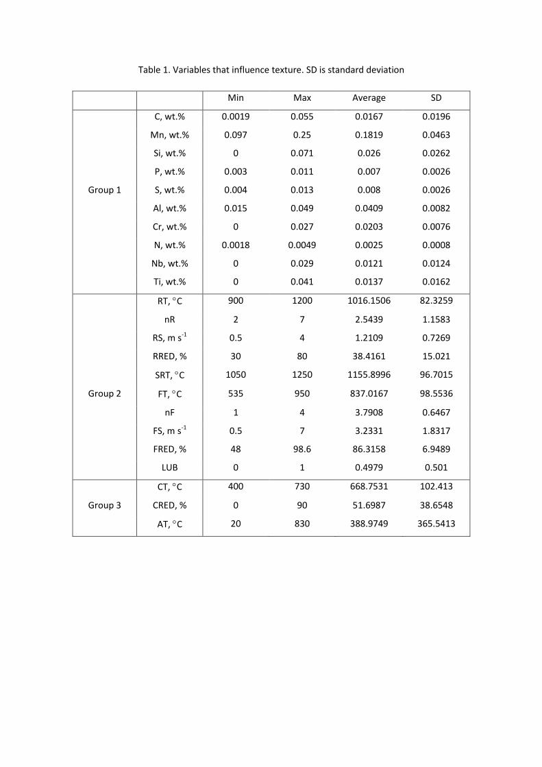
Table 1. Variables that influence texture. SD is standard deviation

Min Max Average SD

C, wt.% 0.0019 0.055 0.0167 0.0196

Mn, wt.% 0.097 0.25 0.1819 0.0463

Si, wt.% 0 0.071 0.026 0.0262

P, wt.% 0.003 0.011 0.007 0.0026

Group 1 S, wt.% 0.004 0.013 0.008 0.0026

Al, wt.% 0.015 0.049 0.0409 0.0082

Cr, wt.% 0 0.027 0.0203 0.0076

N, wt.% 0.0018 0.0049 0.0025 0.0008

Nb, wt.% 0 0.029 0.0121 0.0124

Ti, wt.% 0 0.041 0.0137 0.0162

RT, C 900 1200 1016.1506 82.3259

nR 2 7 2.5439 1.1583

RS, m s-1 0.5 4 1.2109 0.7269

RRED, % 30 80 38.4161 15.021

SRT, C 1050 1250 1155.8996 96.7015

Group 2 FT, C 535 950 837.0167 98.5536

nF 1 4 3.7908 0.6467

FS, m s-1 0.5 7 3.2331 1.8317

FRED, % 48 98.6 86.3158 6.9489

LUB 0 1 0.4979 0.501

CT, C 400 730 668.7531 102.413

Group 3 CRED, % 0 90 51.6987 38.6548

AT, C 20 830 388.9749 365.5413

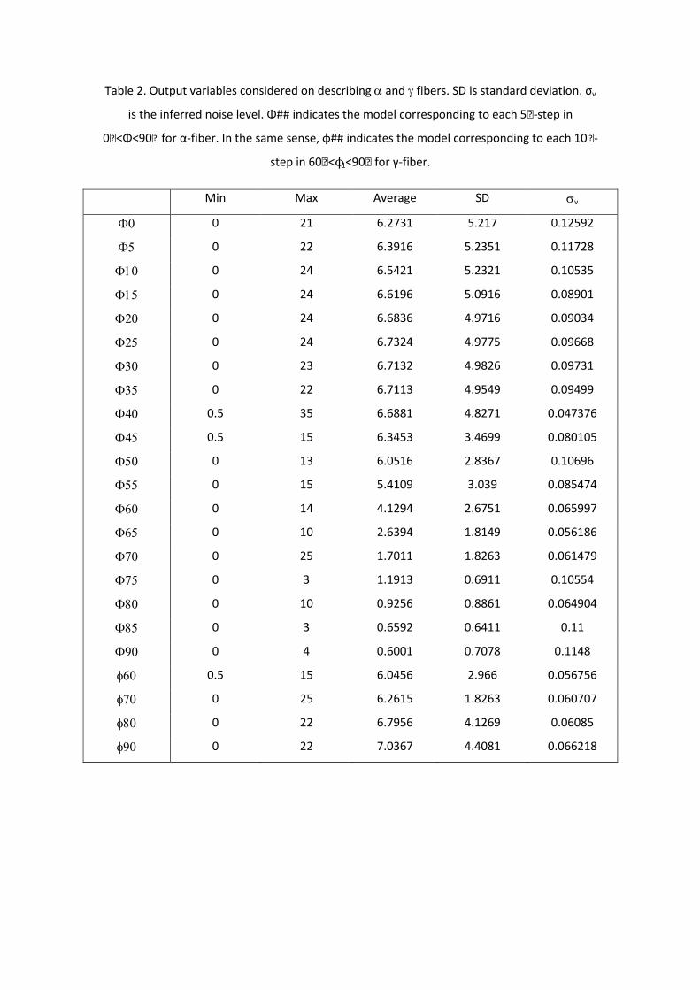
Table 2. Output variables considered on describing and fibers. SD is standard deviation. σv

is the inferred noise level. Φ## indicates the model corresponding to each 5 -ostep in

0 <oΦ<90 ofor α-fiber. In the same sense, φ## indicates the model corresponding to each 10 -o

step in 60 <oϕ1<90 ofor γ-fiber.

Min Max Average SD v

0 21 6.2731 5.217 0.12592

0 22 6.3916 5.2351 0.11728

0 24 6.5421 5.2321 0.10535

0 24 6.6196 5.0916 0.08901

0 24 6.6836 4.9716 0.09034

0 24 6.7324 4.9775 0.09668

0 23 6.7132 4.9826 0.09731

0 22 6.7113 4.9549 0.09499

0.5 35 6.6881 4.8271 0.047376

0.5 15 6.3453 3.4699 0.080105

0 13 6.0516 2.8367 0.10696

0 15 5.4109 3.039 0.085474

0 14 4.1294 2.6751 0.065997

0 10 2.6394 1.8149 0.056186

0 25 1.7011 1.8263 0.061479

0 3 1.1913 0.6911 0.10554

0 10 0.9256 0.8861 0.064904

0 3 0.6592 0.6411 0.11

0 4 0.6001 0.7078 0.1148

0.5 15 6.0456 2.966 0.056756

0 25 6.2615 1.8263 0.060707

0 22 6.7956 4.1269 0.06085

0 22 7.0367 4.4081 0.066218

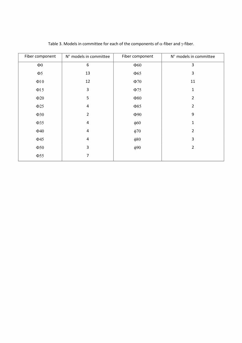
Table 3. Models in committee for each of the components of -fiber and -fiber.

Fiber component N models in committee Fiber component N models in committee

6 3

13 3

12 11

3 1

5 2

4 2

2 9

4 1

4 2

4 3

3 2

7

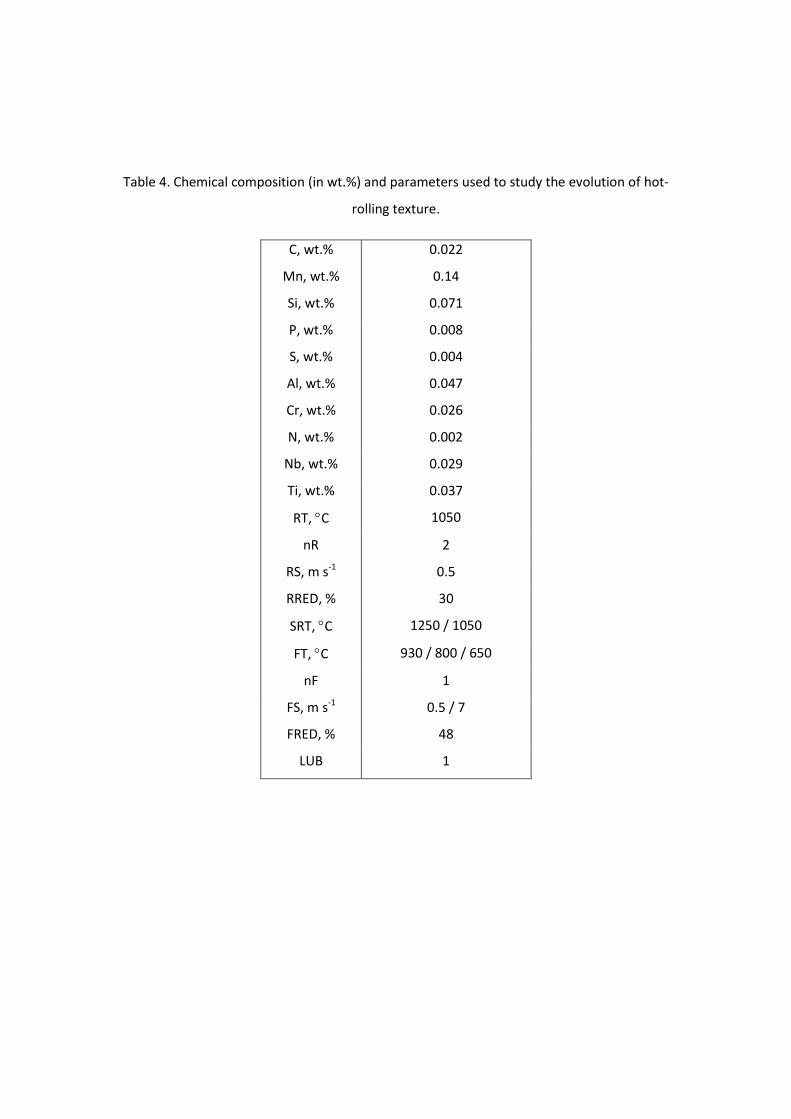
Table 4. Chemical composition (in wt.%) and parameters used to study the evolution of hot-

rolling texture.

C, wt.% 0.022

Mn, wt.% 0.14

Si, wt.% 0.071

P, wt.% 0.008

S, wt.% 0.004

Al, wt.% 0.047

Cr, wt.% 0.026

N, wt.% 0.002

Nb, wt.% 0.029

Ti, wt.% 0.037

RT, C 1050

nR 2

RS, m s-1 0.5

RRED, % 30

SRT, C 1250 / 1050

FT, C 930 / 800 / 650

nF 1

FS, m s-1 0.5 / 7

FRED, % 48

LUB 1

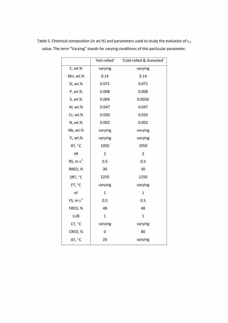
Table 5. Chemical composition (in wt.%) and parameters used to study the evolution of rm

value. The term “Varying” stands for varying conditions of this particular parameter.

‘hot-rolled’ ‘Cold-rolled & Annealed’

C, wt.% varying varying

Mn, wt.% 0.14 0.14

Si, wt.% 0.071 0.071

P, wt.% 0.008 0.008

S, wt.% 0.004 0.0026

Al, wt.% 0.047 0.047

Cr, wt.% 0.026 0.026

N, wt.% 0.002 0.002

Nb, wt.% varying varying

Ti, wt.% varying varying

RT, C 1050 1050

nR 2 2

RS, m s-1 0.5 0.5

RRED, % 30 30

SRT, C 1250 1250

FT, C varying varying

nF 1 1

FS, m s-1 0.5 0.5

FRED, % 48 48

LUB 1 1

CT, C varying varying

CRED, % 0 80

AT, C 20 varying

Figure 1. 2 = 45 section of Euler space showing the ideal BCC rolling and recrystallisation components

Figure 2. Scheme of hot and cold rolling mills for steel production

Figure 3. Variation of inferred noise level (V) as a function of the number of hidden units for = 45 model.

Figure 4. Test error values of the twenty best models for (a) -fiber (Φ between 0 - 20, (b) -fiber (Φ between 25

- 40), (c) -fiber (Φ between 45 - 65), (d) -fiber (Φ between 75 - 90),and (e) -fiber models.

Figure 5. Combined test error values of the committee for (a) -fiber (Φ between 0 - 20), (b) -fiber (Φ between

25 - 40), (c) -fiber (Φ between 45 - 65), (d) -fiber (Φ between 75 - 90),and (e) -fiber models.

Figure 6. Comparison between the predicted and measured values of (a) = 45 and (b) = 60 using their

respective committee of models.

Figure 7. Histogram showing the significance of input variables in influencing the -fiber components perceived by

their respective best models.

Figure 8. Histogram showing the significance of input variables in influencing the -fiber components perceived by

their respective best models.

Figure 9. Influence of SRT on hot-rolling texture (a) alpha and (b) gamma fibre.

Figure 10. Influence of FT on hot-rolling texture (a) alpha and (b) gamma fibre.

Figure 11. Influence of FS on hot-rolling texture (a) alpha and (b) gamma fibre.

Figure 12. Effect of C content on rm.

Figure 13. Effect of Nb content on rm.

Figure 14. Effect of Ti content on rm.

Figure 15. Effect of FT temperature on rm.

Figure 16. Effect of CT temperature on rm.

Figure 17. Effect of AT temperature on rm.

Figure 18. Combined effect of CT and AT on rm value.

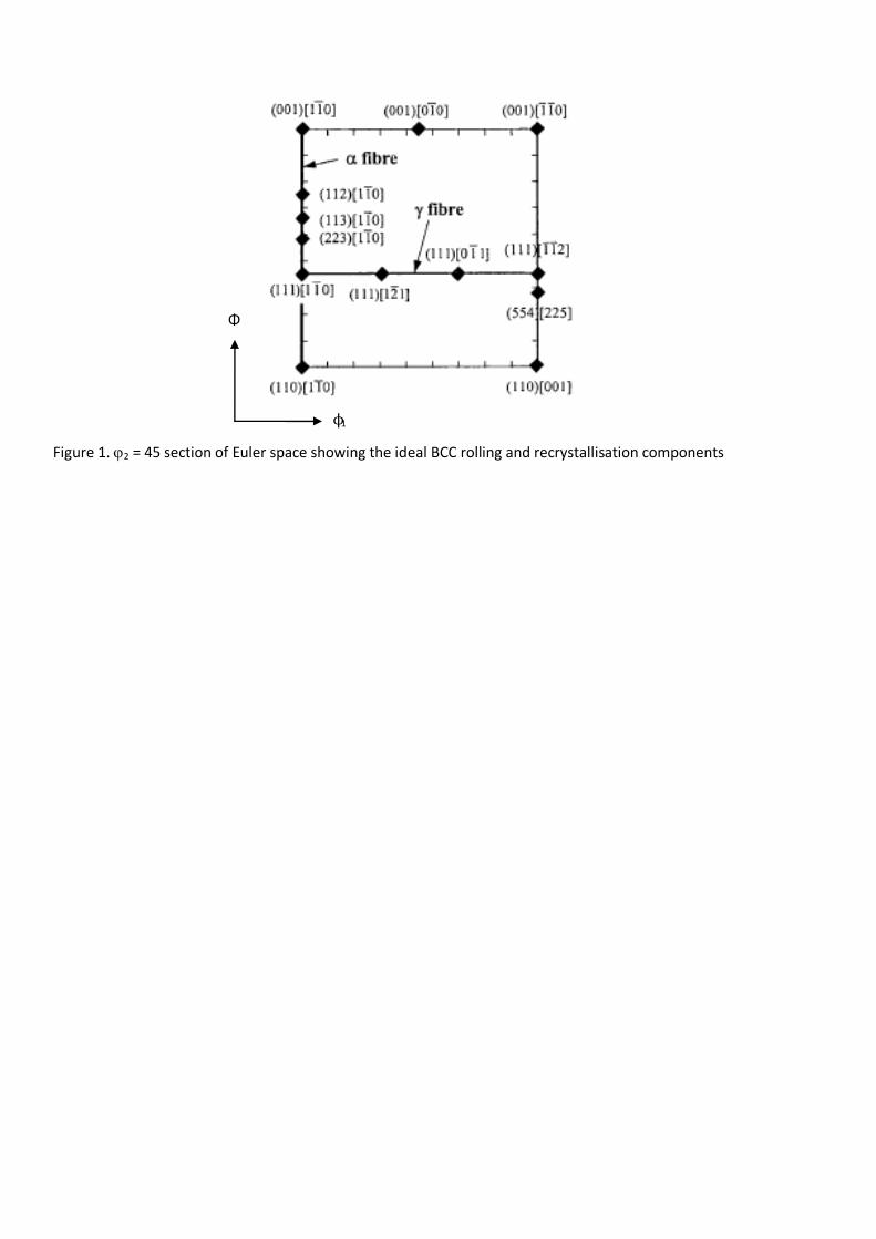
Figure 1. 2 = 45 section of Euler space showing the ideal BCC rolling and recrystallisation components

Φ

ϕ1

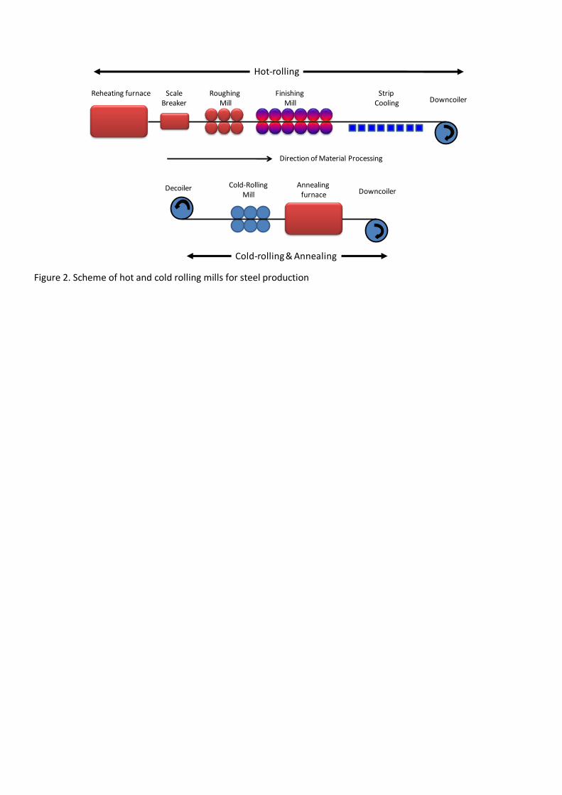
Figure 2. Scheme of hot and cold rolling mills for steel production

Hot-rolling

Cold-rolling& Annealing

Reheating furnace ScaleBreaker

RoughingMill

FinishingMill

StripCooling Downcoiler

Direction of Material Processing

Decoiler Cold-RollingMill

Annealingfurnace Downcoiler

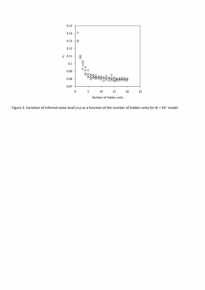
Figure 3. Variation of inferred noise level (V) as a function of the number of hidden units for = 45 model.

0.07

0.08

0.09

0.1

0.11

0.12

0.13

0.14

0.15

0 5 10 15 20 25

v

Number of hidden units

(a) (b)

(c) (d)

(e)

Figure 4. Test error values of the twenty best models for (a) -fiber (Φ between 0 - 20), (b) -fiber (Φ

between 25 - 40), (c) -fiber (Φ between 45 - 65), (d) -fiber (Φ between 75 - 90), and (e) -fiber models.

0

0.2

0.4

0.6

0.8

1

1.2

1.4

1.6

1.8

2

0 5 10 15 20

Test

Err

or

Rank of best model

0

5

10

15

20 0

0.1

0.2

0.3

0.4

0.5

0.6

0.7

0.8

0.9

1

0 5 10 15 20

Test

Err

or

Rank of best model

25

30

35

40

0

0.1

0.2

0.3

0.4

0.5

0.6

0.7

0.8

0.9

1

0 5 10 15 20

Test

Err

or

Rank of best models

45

50

55

60

65 0

0.5

1

1.5

2

2.5

0 5 10 15 20

Test

Err

or

Rank of best models

75

80

85

90

0

0.05

0.1

0.15

0.2

0.25

0.3

0.35

0.4

0.45

0.5

0 5 10 15 20

Test

Err

or

Rank of best model

60

70

80

90

(a) (b)

(c) (d)

(b)

Figure 5. Combined test error values of the committee for (a) -fiber (Φ between 0 - 20), (b) -fiber (Φ

between 25 - 40), (c) -fiber (Φ between 45 - 65), (d) -fiber (Φ between 75 - 90),and (e) -fiber models.

0

0.05

0.1

0.15

0.2

0.25

0.3

0.35

0.4

0.45

0 5 10 15 20

Com

bine

d T

est

Erro

r

Number of models in committee

0

5

10

15

200

0.05

0.1

0.15

0.2

0.25

0.3

0.35

0 5 10 15 20

Com

bine

d T

est

Erro

r

Number of models in committee

25

30

35

40

0

0.05

0.1

0.15

0.2

0.25

0.3

0.35

0.4

0.45

0 5 10 15 20

Com

bine

d T

est

Erro

r

Number of models in committee

45

50

55

60

650

0.1

0.2

0.3

0.4

0.5

0.6

0.7

0 5 10 15 20

Com

bine

d T

est

Erro

r

Number of models in committee

75

80

85

90

0

0.05

0.1

0.15

0.2

0.25

0 5 10 15 20

Com

bine

d T

est

Erro

r

Number of models in committee

60

70

80

90

(a) (b)

Figure 6. Comparison between the predicted and measured values of (a) = 45 and (b) = 60 using their

respective committee of models.

0

2

4

6

8

10

12

14

16

0 2 4 6 8 10 12 14 16

Cal

cula

ted

4

5o

Measured 45o

0

2

4

6

8

10

12

14

0 2 4 6 8 10 12 14

Cal

cula

ted

60

o

Measured 60o

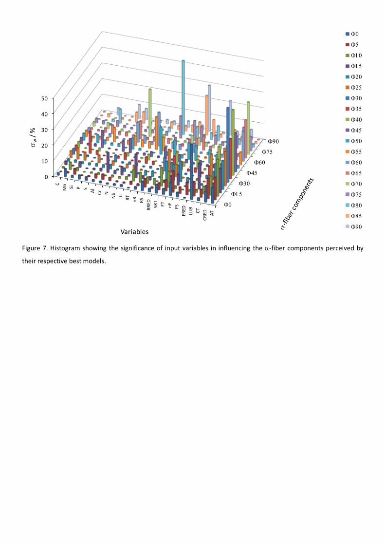
Figure 7. Histogram showing the significance of input variables in influencing the -fiber components perceived by

their respective best models.

0

15

30

45

60

75

90

0

10

20

30

40

50

C

Mn Si P S

Al

Cr N

Nb Ti R

T

nR

RS

RR

ED

SRT

FT nF

FS

FRED

LUB

CT

CR

ED AT

w

/ %

Variables

0

5

10

15

20

25

30

35

40

45

50

55

60

65

70

75

80

85

90

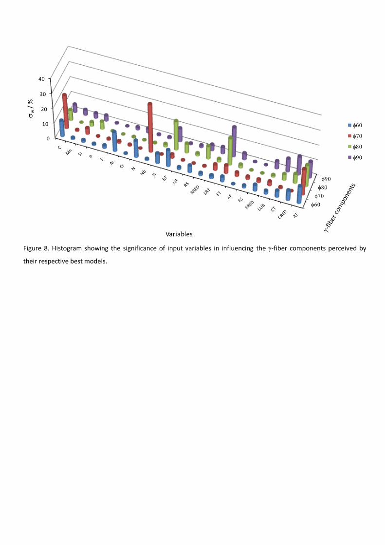
Figure 8. Histogram showing the significance of input variables in influencing the -fiber components perceived by

their respective best models.

60

70

80

90

0

10

20

30

40

w

/ %

Variables

60

70

80

90

(a) (b)

Figure 9. Influence of SRT on hot-rolling texture (a) alpha and (b) gamma fibre.

0

5

10

15

20

25

30

0 5 10 15 20 25 30 35 40 45 50 55 60 65 70 75 80 85 90

f(g)

SRT = 1050 ºC

SRT = 1250 ºC

0

2

4

6

8

10

12

14

60 70 80 90

f(g)

1

SRT = 1250 ºC

SRT = 1050 ºC

(a) (b)

Figure 10. Influence of FT on hot-rolling texture (a) alpha and (b) gamma fibre.

0

5

10

15

20

25

30

0 5 10 15 20 25 30 35 40 45 50 55 60 65 70 75 80 85 90

f(g)

FT = 930 ºC

FT = 800 ºC

FT = 650 ºC

0

2

4

6

8

10

12

14

60 70 80 90

f(g)

1

FT = 930 ºC

FT = 800 ºC

FT = 650 ºC

(a) (b)

Figure 11. Influence of FS on hot-rolling texture (a) alpha and (b) gamma fibre.

0

5

10

15

20

25

30

0 5 10 15 20 25 30 35 40 45 50 55 60 65 70 75 80 85 90

f(g)

FS = 0.5 m/s

FS = 7 m/s

0

2

4

6

8

10

12

14

60 70 80 90

f(g)

1

FS = 0.5 m/s

FS = 7 m/s

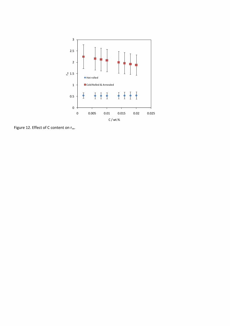
Figure 12. Effect of C content on rm.

0

0.5

1

1.5

2

2.5

3

0 0.005 0.01 0.015 0.02 0.025

r m

C / wt.%

Hot rolled

Cold Rolled & Annealed

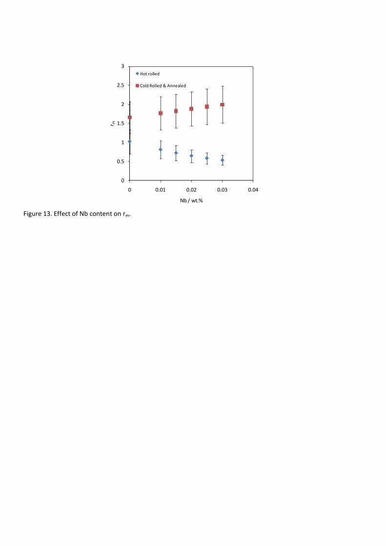
Figure 13. Effect of Nb content on rm.

0

0.5

1

1.5

2

2.5

3

0 0.01 0.02 0.03 0.04

r m

Nb / wt.%

Hot rolled

Cold Rolled & Annealed

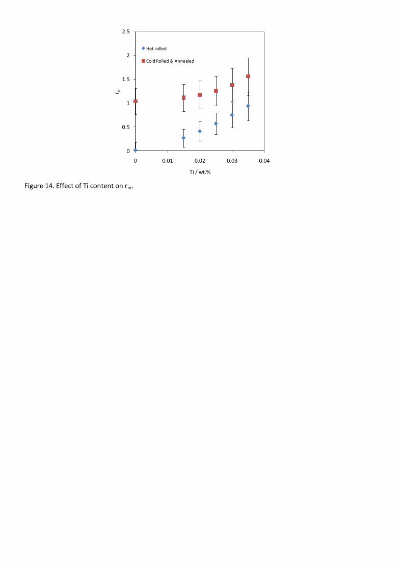
Figure 14. Effect of Ti content on rm.

0

0.5

1

1.5

2

2.5

0 0.01 0.02 0.03 0.04

r m

Ti / wt.%

Hot rolled

Cold Rolled & Annealed

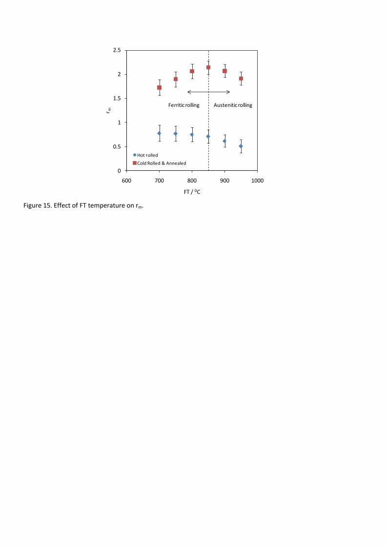
Figure 15. Effect of FT temperature on rm.

0

0.5

1

1.5

2

2.5

600 700 800 900 1000

r m

FT / 0C

Hot rolled

Cold Rolled & Annealed

Austenitic rollingFerritic rolling

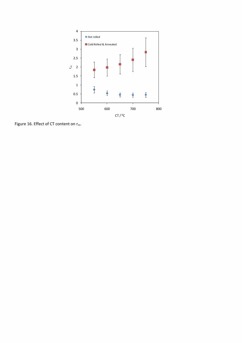
Figure 16. Effect of CT content on rm.

0

0.5

1

1.5

2

2.5

3

3.5

4

500 600 700 800

r m

CT / 0C

Hot rolled

Cold Rolled & Annealed

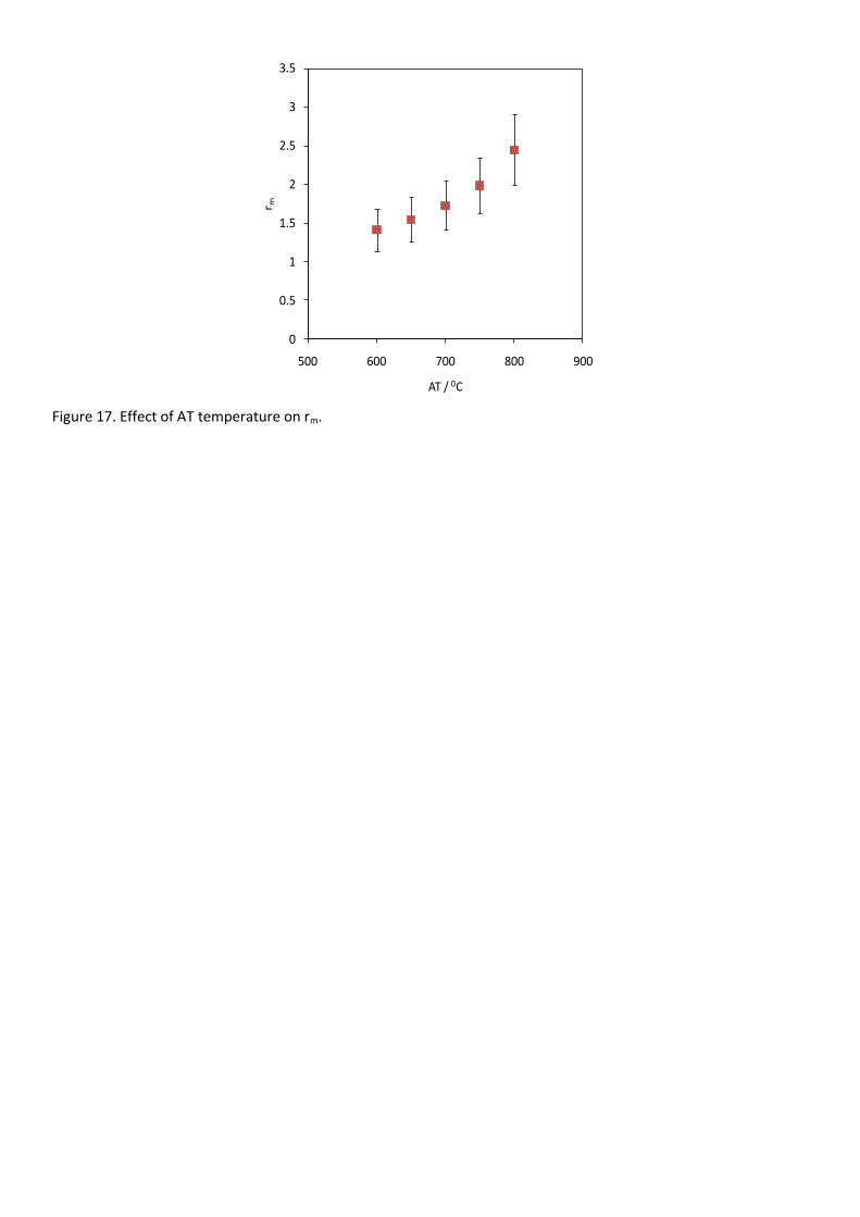
Figure 17. Effect of AT temperature on rm.

0

0.5

1

1.5

2

2.5

3

3.5

500 600 700 800 900

r m

AT / 0C

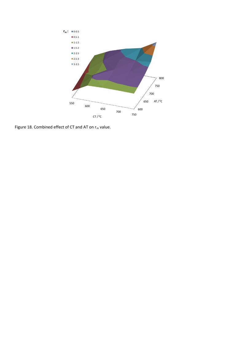
Figure 18. Combined effect of CT and AT on rm value.

600

650

700

750

800

550600

650700

750

AT / 0C

CT / 0C

rm : 0-0.5

0.5-1

1-1.5

1.5-2

2-2.5

2.5-3

3-3.5