Dense Associative Memory for Pattern Recognition
Dmitry KrotovSimons Center for Systems Biology
Institute for Advanced StudyPrinceton, [email protected]
John J. HopfieldPrinceton Neuroscience Institute
Princeton UniversityPrinceton, USA
Abstract
A model of associative memory is studied, which stores and reliably retrieves manymore patterns than the number of neurons in the network. We propose a simpleduality between this dense associative memory and neural networks commonly usedin deep learning. On the associative memory side of this duality, a family of modelsthat smoothly interpolates between two limiting cases can be constructed. One limitis referred to as the feature-matching mode of pattern recognition, and the otherone as the prototype regime. On the deep learning side of the duality, this familycorresponds to feedforward neural networks with one hidden layer and variousactivation functions, which transmit the activities of the visible neurons to thehidden layer. This family of activation functions includes logistics, rectified linearunits, and rectified polynomials of higher degrees. The proposed duality makesit possible to apply energy-based intuition from associative memory to analyzecomputational properties of neural networks with unusual activation functions – thehigher rectified polynomials which until now have not been used in deep learning.The utility of the dense memories is illustrated for two test cases: the logical gateXOR and the recognition of handwritten digits from the MNIST data set.
1 Introduction
Pattern recognition and models of associative memory [1] are closely related. Consider imageclassification as an example of pattern recognition. In this problem, the network is presented with animage and the task is to label the image. In the case of associative memory the network stores a set ofmemory vectors. In a typical query the network is presented with an incomplete pattern resembling,but not identical to, one of the stored memories and the task is to recover the full memory. Pixelintensities of the image can be combined together with the label of that image into one vector [2],which will serve as a memory for the associative memory. Then the image itself can be thought ofas a partial memory cue. The task of identifying an appropriate label is a subpart of the associativememory reconstruction. There is a limitation in using this idea to do pattern recognition. The standardmodel of associative memory works well in the limit when the number of stored patterns is muchsmaller than the number of neurons [1], or equivalently the number of pixels in an image. In orderto do pattern recognition with small error rate one would need to store many more memories thanthe typical number of pixels in the presented images. This is a serious problem. It can be solved bymodifying the standard energy function of associative memory, quadratic in interactions between theneurons, by including in it higher order interactions. By properly designing the energy function (orHamiltonian) for these models with higher order interactions one can store and reliably retrieve manymore memories than the number of neurons in the network.
Deep neural networks have proven to be useful for a broad range of problems in machine learningincluding image classification, speech recognition, object detection, etc. These models are composedof several layers of neurons, so that the output of one layer serves as the input to the next layer. Each
30th Conference on Neural Information Processing Systems (NIPS 2016), Barcelona, Spain.
neuron calculates a weighted sum of the inputs and passes the result through a non-linear activationfunction. Traditionally, deep neural networks used activation functions such as hyperbolic tangents orlogistics. Learning the weights in such networks, using a backpropagation algorithm, faced seriousproblems in the 1980s and 1990s. These issues were largely resolved by introducing unsupervisedpre-training, which made it possible to initialize the weights in such a way that the subsequentbackpropagation could only gently move boundaries between the classes without destroying thefeature detectors [3, 4]. More recently, it was realized that the use of rectified linear units (ReLU)instead of the logistic functions speeds up learning and improves generalization [5, 6, 7]. Rectifiedlinear functions are usually interpreted as firing rates of biological neurons. These rates are equalto zero if the input is below a certain threshold and linearly grow with the input if it is above thethreshold. To mimic biology the output should be small or zero if the input is below the threshold, butit is much less clear what the behavior of the activation function should be for inputs exceeding thethreshold. Should it grow linearly, sub-linearly, or faster than linearly? How does this choice affectthe computational properties of the neural network? Are there other functions that would work evenbetter than the rectified linear units? These questions to the best of our knowledge remain open.
This paper examines these questions through the lens of associative memory. We start by discussinga family of models of associative memory with large capacity. These models use higher order (higherthan quadratic) interactions between the neurons in the energy function. The associative memorydescription is then mapped onto a neural network with one hidden layer and an unusual activationfunction, related to the Hamiltonian. We show that by varying the power of interaction vertex inthe energy function (or equivalently by changing the activation function of the neural network) onecan force the model to learn representations of the data either in terms of features or in terms ofprototypes.
2 Associative memory with large capacity
The standard model of associative memory [1] uses a system of N binary neurons, with values ±1. Aconfiguration of all the neurons is denoted by a vector �
i
. The model stores K memories, denoted by⇠
µ
i
, which for the moment are also assumed to be binary. The model is defined by an energy function,which is given by
E = �1
2
NX
i,j=1
�
i
T
ij
�
j
, T
ij
=
KX
µ=1
⇠
µ
i
⇠
µ
j
, (1)
and a dynamical update rule that decreases the energy at every update. The basic problem is thefollowing: when presented with a new pattern the network should respond with a stored memorywhich most closely resembles the input.
There has been a large amount of work in the community of statistical physicists investigatingthe capacity of this model, which is the maximal number of memories that the network can storeand reliably retrieve. It has been demonstrated [1, 8, 9] that in case of random memories thismaximal value is of the order of K
max ⇡ 0.14N . If one tries to store more patterns, severalneighboring memories in the configuration space will merge together producing a ground state ofthe Hamiltonian (1), which has nothing to do with any of the stored memories. By modifying theHamiltonian (1) in a way that removes second order correlations between the stored memories, it ispossible [10] to improve the capacity to K
max
= N .
The mathematical reason why the model (1) gets confused when many memories are stored is thatseveral memories produce contributions to the energy which are of the same order. In other words theenergy decreases too slowly as the pattern approaches a memory in the configuration space. In orderto take care of this problem, consider a modification of the standard energy
E = �KX
µ=1
F
�⇠
µ
i
�
i
�(2)
In this formula F (x) is some smooth function (summation over index i is assumed). The compu-tational capabilities of the model will be illustrated for two cases. First, when F (x) = x
n (n isan integer number), which is referred to as a polynomial energy function. Second, when F (x) is a
2

rectified polynomial energy function
F (x) =
⇢x
n
, x � 0
0, x < 0
(3)
In the case of the polynomial function with n = 2 the network reduces to the standard model ofassociative memory [1]. If n > 2 each term in (2) becomes sharper compared to the n = 2 case, thusmore memories can be packed into the same configuration space before cross-talk intervenes.
Having defined the energy function one can derive an iterative update rule that leads to decrease ofthe energy. We use asynchronous updates flipping one unit at a time. The update rule is:
�
(t+1)i
= Sign
KX
µ=1
✓F
⇣⇠
µ
i
+
X
j 6=i
⇠
µ
j
�
(t)j
⌘� F
⇣� ⇠
µ
i
+
X
j 6=i
⇠
µ
j
�
(t)j
⌘◆�, (4)
The argument of the sign function is the difference of two energies. One, for the configuration withall but the i-th units clumped to their current states and the i-th unit in the “off” state. The other onefor a similar configuration, but with the i-th unit in the “on” state. This rule means that the systemupdates a unit, given the states of the rest of the network, in such a way that the energy of the entireconfiguration decreases. For the case of polynomial energy function a very similar family of modelswas considered in [11, 12, 13, 14, 15, 16]. The update rule in those models was based on the inducedmagnetic fields, however, and not on the difference of energies. The two are slightly different due tothe presence of self-coupling terms. Throughout this paper we use energy-based update rules.
How many memories can model (4) store and reliably retrieve? Consider the case of random patterns,so that each element of the memories is equal to ±1 with equal probability. Imagine that the systemis initialized in a state equal to one of the memories (pattern number µ). One can derive a stabilitycriterion, i.e. the upper bound on the number of memories such that the network stays in that initialstate. Define the energy difference between the initial state and the state with spin i flipped
�E =
KX
⌫=1
⇣⇠
⌫
i
⇠
µ
i
+
X
j 6=i
⇠
⌫
j
⇠
µ
j
⌘n
�KX
⌫=1
⇣� ⇠
⌫
i
⇠
µ
i
+
X
j 6=i
⇠
⌫
j
⇠
µ
j
⌘n
,
where the polynomial energy function is used. This quantity has a mean h�Ei = N
n � (N � 2)
n ⇡2nN
n�1, which comes from the term with ⌫ = µ, and a variance (in the limit of large N )⌃
2= ⌦
n
(K � 1)N
n�1, where ⌦
n
= 4n
2(2n � 3)!!
The i-th bit becomes unstable when the magnitude of the fluctuation exceeds the energy gap h�Eiand the sign of the fluctuation is opposite to the sign of the energy gap. Thus the probability that thestate of a single neuron is unstable (in the limit when both N and K are large, so that the noise iseffectively gaussian) is equal to
Perror =
1Z
h�Ei
dxp2⇡⌃
2e
� x
2
2⌃2 ⇡r
(2n � 3)!!
2⇡
K
N
n�1e
� N
n�1
2K(2n�3)!!
Requiring that this probability is less than a small value, say 0.5%, one can find the upper limit onthe number of patterns that the network can store
K
max
= ↵
n
N
n�1, (5)
where ↵
n
is a numerical constant, which depends on the (arbitrary) threshold 0.5%. The casen = 2 corresponds to the standard model of associative memory and gives the well known resultK = 0.14N . For the perfect recovery of a memory (Perror < 1/N ) one obtains
K
max
no errors ⇡ 1
2(2n � 3)!!
N
n�1
ln(N)
(6)
For higher powers n the capacity rapidly grows with N in a non-linear way, allowing the networkto store and reliably retrieve many more patterns than the number of neurons that it has, in accord1
with [13, 14, 15, 16]. This non-linear scaling relationship between the capacity and the size of thenetwork is the phenomenon that we exploit.
1The n-dependent coefficient in (6) depends on the exact form of the Hamiltonian and the update rule.References [13, 14, 15] do not allow repeated indices in the products over neurons in the energy function,therefore obtain a different coefficient. In [16] the Hamiltonian coincides with ours, but the update rule isdifferent, which, however, results in exactly the same coefficient as in (6).
3

We study a family of models of this kind as a function of n. At small n many terms contribute to thesum over µ in (2) approximately equally. In the limit n ! 1 the dominant contribution to the sumcomes from a single memory, which has the largest overlap with the input. It turns out that optimalcomputation occurs in the intermediate range.
3 The case of XOR
The case of XOR is elementary, yet instructive. It is presented here for three reasons. First, it illustratesthe construction (2) in this simplest case. Second, it shows that as n increases, the computationalcapabilities of the network also increase. Third, it provides the simplest example of a situation inwhich the number of memories is larger than the number of neurons, yet the network works reliably.
The problem is the following: given two inputs x and y produce an output z such that the truth table
x y z
-1 -1 -1-1 1 11 -1 11 1 -1
is satisfied. We will treat this task as an associative memory problem and will simply embed thefour examples of the input-output triplets x, y, z in the memory. Therefore the network has N = 3
identical units: two of which will be used for the inputs and one for the output, and K = 4 memories⇠
µ
i
, which are the four lines of the truth table. Thus, the energy (2) is equal to
E
n
(x, y, z) = ��
� x � y � z
�n �
�� x + y + z
�n �
�x � y + z
�n �
�x + y � z
�n
, (7)
where the energy function is chosen to be a polynomial of degree n. For odd n, energy (7) is an oddfunction of each of its arguments, E
n
(x, y, �z) = �E
n
(x, y, z). For even n, it is an even function.For n = 1 it is equal to zero. Thus, if evaluated on the corners of the cube x, y, z = ±1, it reduces to
E
n
(x, y, z) =
8<
:
0, n = 1
C
n
, n = 2, 4, 6, ...
C
n
xyz, n = 3, 5, 7, ...,
(8)
where coefficients C
n
denote numerical constants.
In order to solve the XOR problem one can present to the network an “incomplete pattern” of inputs(x, y) and let the output z adjust to minimize the energy of the three-spin configuration, while holdingthe inputs fixed. The network clearly cannot solve this problem for n = 1 and n = 2, since the energydoes not depend on the spin configuration. The case n = 2 is the standard model of associativememory. It can also be thought of as a linear perceptron, and the inability to solve this problemrepresents the well known statement [17] that linear perceptrons cannot compute XOR without hiddenneurons. The case of odd n � 3 provides an interesting solution. Given two inputs, x and y, one canchoose the output z that minimizes the energy. This leads to the update rule
z = Sign
⇥E
n
(x, y, �1) � E
n
(x, y, +1)
⇤= Sign
⇥� xy
⇤
Thus, in this simple case the network is capable of solving the problem for higher odd values of n,while it cannot do so for n = 1 and n = 2. In case of rectified polynomials, a similar constructionsolves the problem for any n � 2. The network works well in spite of the fact that K > N .
4 An example of a pattern recognition problem, the case of MNIST
The MNIST data set is a collection of handwritten digits, which has 60000 training examples and10000 test images. The goal is to classify the digits into 10 classes. The visible neurons, one for eachpixel, are combined together with 10 classification neurons in one vector that defines the state ofthe network. The visible part of this vector is treated as an “incomplete” pattern and the associativememory is allowed to calculate a completion of that pattern, which is the label of the image.
Dense associative memory (2) is a recurrent network in which every neuron can be updated multipletimes. For the purposes of digit classification, however, this model will be used in a very limited
4

capacity, allowing it to perform only one update of the classification neurons. The network isinitialized in the state when the visible units v
i
are clamped to the intensities of a given image and theclassification neurons are in the off state x
↵
= �1 (see Fig.1A). The network is allowed to makeone update of the classification neurons, while keeping the visible units clamped, to produce theoutput c
↵
. The update rule is similar to (4) except that the sign is replaced by the continuous functiong(x) = tanh(x)
c
↵
= g
�
KX
µ=1
✓F
⇣� ⇠
µ
↵
x
↵
+
X
� 6=↵
⇠
µ
�
x
�
+
NX
i=1
⇠
µ
i
v
i
⌘�F
⇣⇠
µ
↵
x
↵
+
X
� 6=↵
⇠
µ
�
x
�
+
NX
i=1
⇠
µ
i
v
i
⌘◆�, (9)
where parameter � regulates the slope of g(x). The proposed digit class is given by the numberof a classification neuron producing the maximal output. Throughout this section the rectifiedpolynomials (3) are used as functions F . To learn effective memories for use in pattern classification,an objective function is defined (see Appendix A in Supplemental), which penalizes the discrepancyA B
v
i
c
↵
v
i
x
↵
0 500 1000 1500 2000 2500 3000
1.4
1.5
1.6
1.7
1.8
1.9
2er
ror,
test
set
Epochs number of epochsnumber of epochs
test
err
or, %
test
err
or, %
0 500 1000 1500 2000 2500 3000
1.4
1.5
1.6
1.7
1.8
1.9
2
erro
r, te
st s
et
Epochs
158-262 epochs
n = 3
n = 2
179-312 epochs
Figure 1: (A) The network has N = 28 ⇥ 28 = 784 visible neurons and Nc = 10 classification neurons.The visible units are clamped to intensities of pixels (which is mapped on the segment [�1, 1]), while theclassification neurons are initialized in the state x↵ and then updated once to the state c↵. (B) Behavior of theerror on the test set as training progresses. Each curve corresponds to a different combination of hyperparametersfrom the optimal window, which was determined on the validation set. The arrows show the first time when theerror falls below a 2% threshold. All models have K = 2000 memories (hidden units).
between the output c
↵
and the target output. This objective function is then minimized using abackpropagation algorithm. The learning starts with random memories drawn from a Gaussiandistribution. The backpropagation algorithm then finds a collection of K memories ⇠
µ
i,↵
, whichminimize the classification error on the training set. The memories are normalized to stay within the�1 ⇠
µ
i,↵
1 range, absorbing their overall scale into the definition of the parameter �.
The performance of the proposed classification framework is studied as a function of the power n.The next section shows that a rectified polynomial of power n in the energy function is equivalentto the rectified polynomial of power n � 1 used as an activation function in a feedforward neuralnetwork with one hidden layer of neurons. Currently, the most common choice of activation functionsfor training deep neural networks is the ReLU, which in our language corresponds to n = 2 forthe energy function. Although not currently used to train deep networks, the case n = 3 wouldcorrespond to a rectified parabola as an activation function. We start by comparing the performancesof the dense memories in these two cases.
The performance of the network depends on n and on the remaining hyperparameters, thus the hyper-parameters should be optimized for each value of n. In order to test the variability of performancesfor various choices of hyperparameters at a given n, a window of hyperparameters for which thenetwork works well on the validation set (see the Appendix A in Supplemental) was determined.Then many networks were trained for various choices of the hyperparameters from this window toevaluate the performance on the test set. The test errors as training progresses are shown in Fig.1B.While there is substantial variability among these samples, on average the cluster of trajectories forn = 3 achieves better results on the test set than that for n = 2. These error rates should be comparedwith error rates for backpropagation alone without the use of generative pretraining, various kindsof regularizations (for example dropout) or adversarial training, all of which could be added to ourconstruction if necessary. In this class of models the best published results are all2 in the 1.6% range[18], see also controls in [19, 20]. This agrees with our results for n = 2. The n = 3 case doesslightly better than that as is clear from Fig.1B, with all the samples performing better than 1.6%.
2Although there are better results on pixel permutation invariant task, see for example [19, 20, 21, 22].
5

Higher rectified polynomials are also faster in training compared to ReLU. For the n = 2 case, theerror crosses the 2% threshold for the first time during training in the range of 179-312 epochs. Forthe n = 3 case, this happens earlier on average, between 158-262 epochs. For higher powers n
this speed-up is larger. This is not a huge effect for a small dataset such as MNIST. However, thisspeed-up might be very helpful for training large networks on large datasets, such as ImageNet. Asimilar effect was reported earlier for the transition between saturating units, such as logistics orhyperbolic tangents, to ReLU [7]. In our family of models that result corresponds to moving fromn = 1 to n = 2.
Feature to prototype transition
How does the computation performed by the neural network change as n varies? There are twoextreme classes of theories of pattern recognition: feature-matching and formation of a prototype.According to the former, an input is decomposed into a set of features, which are compared withthose stored in the memory. The subset of the stored features activated by the presented input is theninterpreted as an object. One object has many features; features can also appear in more than oneobject. The prototype theory provides an alternative approach, in which objects are recognized as awhole. The prototypes do not necessarily match the object exactly, but rather are blurred abstract
64
128
192
256
64
128
192
256
64
128
192
256
64
128
192
256
0 1 2 3 4 5 6 7 8 9 100
10
20
30
40
50
perc
ent o
f act
ive
mem
orie
s
number of strongly positively driven RU
n=2n=3n=20n=30
1 2 3 4 5 6 7 8 9 10 11 120
2000
4000
6000
8000
10000
num
ber o
f tes
t im
ages
number of memories strongly contributing to the correct RU
n=2n=3n=20n=30
64
128
192
256
number of RU with ⇠µ
↵
> 0.99 number of memories making the decision
perc
ent o
f mem
orie
s, %
num
ber
of te
st im
ages
�1
�0.5
0.5
0
1
n = 2
n = 3 n = 20 n = 30
errortest = 1.51%
errortest = 1.44%
errortest = 1.61%
errortest = 1.80%
Figure 2: We show 25 randomly selected memories (feature detectors) for four networks, which use recti-fied polynomials of degrees n = 2, 3, 20, 30 as the energy function. The magnitude of a memory elementcorresponding to each pixel is plotted in the location of that pixel, the color bar explains the color code. Thehistograms at the bottom are explained in the text. The error rates refer to the particular four samples used in thisfigure. RU stands for recognition unit.
representations which include all the features that an object has. We argue that the computationalmodels proposed here describe feature-matching mode of pattern recognition for small n and theprototype regime for large n. This can be anticipated from the sharpness of contributions that eachmemory makes to the total energy (2). For large n the function F (x) peaks much more sharplyaround each memory compared to the case of small n. Thus, at large n all the information about adigit must be written in only one memory, while at small n this information can be distributed amongseveral memories. In the case of intermediate n some learned memories behave like features whileothers behave like prototypes. These two classes of memories work together to model the data in anefficient way.
The feature to prototype transition is clearly seen in memories shown in Fig.2. For n = 2 or 3
each memory does not look like a digit, but resembles a pattern of activity that might be useful forrecognizing several different digits. For n = 20 many of the memories can be recognized as digits,which are surrounded by white margins representing elements of memories having approximatelyzero values. These margins describe the variability of thicknesses of lines of different trainingexamples and mathematically mean that the energy (2) does not depend on whether the correspondingpixel is on or off. For n = 30 most of the memories represent prototypes of whole digits or largeportions of digits, with a small admixture of feature memories that do not resemble any digit.
6

The feature to prototype transition can be visualized by showing the feature detectors in situationswhen there is a natural ordering of pixels. Such ordering exists in images, for example. In generalsituations, however, there is no preferred permutation of visible neurons that would reveal thisstructure (e.g. in the case of genomic data). It is therefore useful to develop a measure that permits adistinction to be made between features and prototypes in the absence of such visual space. Towardsthe end of training most of the recognition connections ⇠
µ
↵
are approximately equal to ±1. Onecan choose an arbitrary cutoff, and count the number of recognition connections that are in the “on”state (⇠µ
↵
= +1) for each memory. The distribution function of this number is shown on the lefthistogram in Fig.2. Intuitively, this quantity corresponds to the number of different digit classesthat a particular memory votes for. At small n, most of the memories vote for three to five differentdigit classes, a behavior characteristic of features. As n increases, each memory specializes andvotes for only a single class. In the case n = 30, for example, more than 40% of memories vote foronly one class, a behavior characteristic of prototypes. A second way to see the feature to prototypetransition is to look at the number of memories which make large contributions to the classificationdecision (right histogram in Fig.2). For each test image one can find the memory that makes thelargest contribution to the energy gap, which is the sum over µ in (9). Then one can count the numberof memories that contribute to the gap by more than 0.9 of this largest contribution. For small n,there are many memories that satisfy this criterion and the distribution function has a long tail. Inthis regime several memories are cooperating with each other to make a classification decision. Forn = 30, however, more than 8000 of 10000 test images do not have a single other memory that wouldmake a contribution comparable with the largest one. This result is not sensitive to the arbitrary choice(0.9) of the cutoff. Interestingly, the performance remains competitive even for very large n ⇡ 20
(see Fig.2) in spite of the fact that these networks are doing a very different kind of computationcompared with that at small n.
5 Relationship to a neural network with one hidden layer
In this section we derive a simple duality between the dense associative memory and a feedforwardneural network with one layer of hidden neurons. In other words, we show that the same computationalmodel has two very different descriptions: one in terms of associative memory, the other one in terms
v
i
c
↵
v
i
v
i
c
↵
f
g
h
µ
x
↵
= �"
Figure 3: On the left a feedforward neural network with one layer of hidden neurons. The states of the visibleunits are transformed to the hidden neurons using a non-linear function f , the states of the hidden units aretransformed to the output layer using a non-linear function g. On the right the model of dense associativememory with one step update (9). The two models are equivalent.
of a network with one layer of hidden units. Using this correspondence one can transform the familyof dense memories, constructed for different values of power n, to the language of models used indeep learning. The resulting neural networks are guaranteed to inherit computational properties ofthe dense memories such as the feature to prototype transition.
The construction is very similar to (9), except that the classification neurons are initialized in the statewhen all of them are equal to �", see Fig.3. In the limit " ! 0 one can expand the function F in (9)so that the dominant contribution comes from the term linear in ". Then
c
↵
⇡ g
h�
KX
µ=1
F
0⇣ NX
i=1
⇠
µ
i
v
i
⌘(�2⇠
µ
↵
x
↵
)
i= g
h KX
µ=1
⇠
µ
↵
F
0�⇠
µ
i
v
i
�i= g
h KX
µ=1
⇠
µ
↵
f
�⇠
µ
i
v
i
�i, (10)
where the parameter � is set to � = 1/(2") (summation over the visible index i is assumed). Thus,the model of associative memory with one step update is equivalent to a conventional feedforwardneural network with one hidden layer provided that the activation function from the visible layer tothe hidden layer is equal to the derivative of the energy function
f(x) = F
0(x) (11)
7
The visible part of each memory serves as an incoming weight to the hidden layer, and the recognitionpart of the memory serves as an outgoing weight from the hidden layer. The expansion used in (10)
is justified by a conditionNP
i=1⇠
µ
i
v
i
�N
cP↵=1
⇠
µ
↵
x
↵
, which is satisfied for most common problems, and
is simply a statement that labels contain far less information than the data itself3.
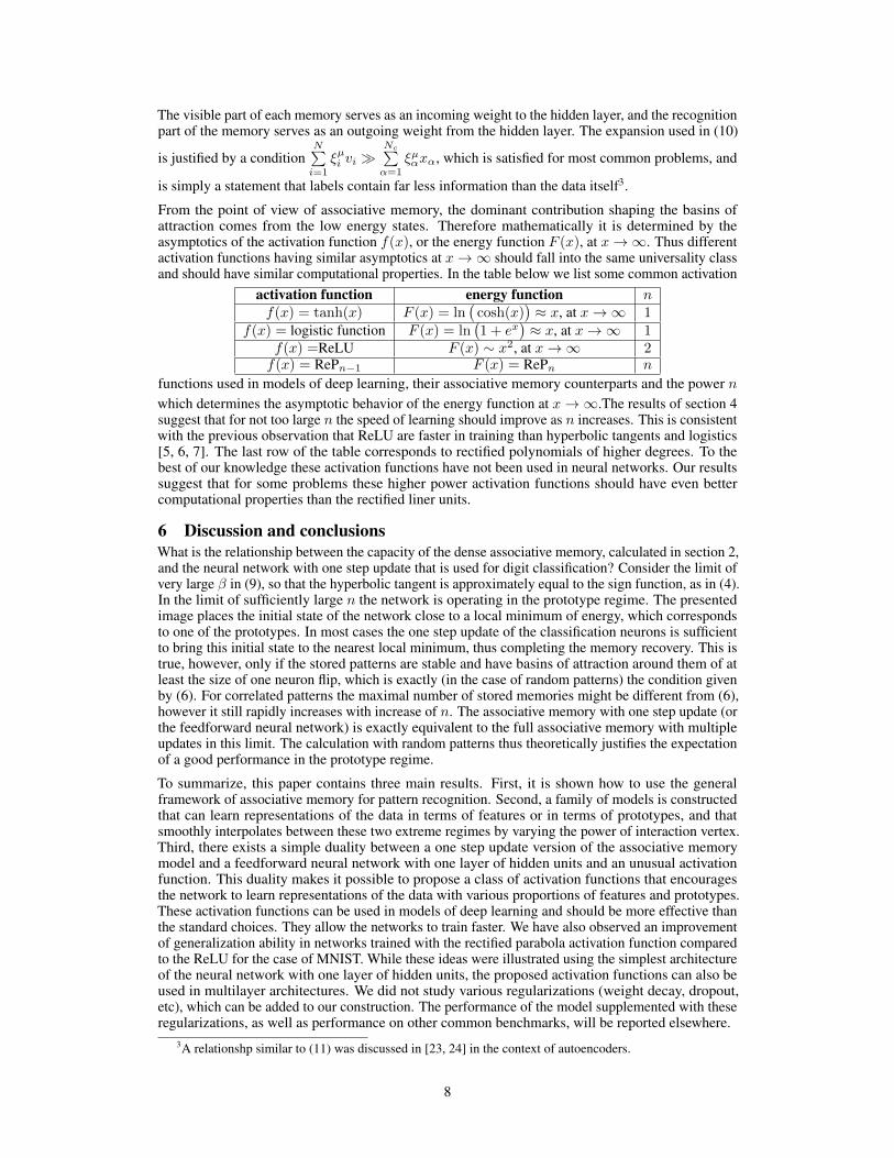
From the point of view of associative memory, the dominant contribution shaping the basins ofattraction comes from the low energy states. Therefore mathematically it is determined by theasymptotics of the activation function f(x), or the energy function F (x), at x ! 1. Thus differentactivation functions having similar asymptotics at x ! 1 should fall into the same universality classand should have similar computational properties. In the table below we list some common activation
activation function energy function n
f(x) = tanh(x) F (x) = ln
�cosh(x)
�⇡ x, at x ! 1 1
f(x) = logistic function F (x) = ln
�1 + e
x
�⇡ x, at x ! 1 1
f(x) =ReLU F (x) ⇠ x
2, at x ! 1 2
f(x) = RePn�1 F (x) = ReP
n
n
functions used in models of deep learning, their associative memory counterparts and the power n
which determines the asymptotic behavior of the energy function at x ! 1.The results of section 4suggest that for not too large n the speed of learning should improve as n increases. This is consistentwith the previous observation that ReLU are faster in training than hyperbolic tangents and logistics[5, 6, 7]. The last row of the table corresponds to rectified polynomials of higher degrees. To thebest of our knowledge these activation functions have not been used in neural networks. Our resultssuggest that for some problems these higher power activation functions should have even bettercomputational properties than the rectified liner units.
6 Discussion and conclusionsWhat is the relationship between the capacity of the dense associative memory, calculated in section 2,and the neural network with one step update that is used for digit classification? Consider the limit ofvery large � in (9), so that the hyperbolic tangent is approximately equal to the sign function, as in (4).In the limit of sufficiently large n the network is operating in the prototype regime. The presentedimage places the initial state of the network close to a local minimum of energy, which correspondsto one of the prototypes. In most cases the one step update of the classification neurons is sufficientto bring this initial state to the nearest local minimum, thus completing the memory recovery. This istrue, however, only if the stored patterns are stable and have basins of attraction around them of atleast the size of one neuron flip, which is exactly (in the case of random patterns) the condition givenby (6). For correlated patterns the maximal number of stored memories might be different from (6),however it still rapidly increases with increase of n. The associative memory with one step update (orthe feedforward neural network) is exactly equivalent to the full associative memory with multipleupdates in this limit. The calculation with random patterns thus theoretically justifies the expectationof a good performance in the prototype regime.
To summarize, this paper contains three main results. First, it is shown how to use the generalframework of associative memory for pattern recognition. Second, a family of models is constructedthat can learn representations of the data in terms of features or in terms of prototypes, and thatsmoothly interpolates between these two extreme regimes by varying the power of interaction vertex.Third, there exists a simple duality between a one step update version of the associative memorymodel and a feedforward neural network with one layer of hidden units and an unusual activationfunction. This duality makes it possible to propose a class of activation functions that encouragesthe network to learn representations of the data with various proportions of features and prototypes.These activation functions can be used in models of deep learning and should be more effective thanthe standard choices. They allow the networks to train faster. We have also observed an improvementof generalization ability in networks trained with the rectified parabola activation function comparedto the ReLU for the case of MNIST. While these ideas were illustrated using the simplest architectureof the neural network with one layer of hidden units, the proposed activation functions can also beused in multilayer architectures. We did not study various regularizations (weight decay, dropout,etc), which can be added to our construction. The performance of the model supplemented with theseregularizations, as well as performance on other common benchmarks, will be reported elsewhere.
3A relationshp similar to (11) was discussed in [23, 24] in the context of autoencoders.
8

References[1] Hopfield, J.J., 1982. Neural networks and physical systems with emergent collective computational
abilities. Proceedings of the national academy of sciences, 79(8), pp.2554-2558.[2] LeCun, Y., Chopra, S., Hadsell, R., Ranzato, M. and Huang, F., 2006. A tutorial on energy-based learning.
Predicting structured data, 1, p.0.[3] Hinton, G.E., Osindero, S. and Teh, Y.W., 2006. A fast learning algorithm for deep belief nets. Neural
computation, 18(7), pp.1527-1554.[4] Hinton, G.E. and Salakhutdinov, R.R., 2006. Reducing the dimensionality of data with neural networks.
Science, 313(5786), pp.504-507.[5] Nair, V. and Hinton, G.E., 2010. Rectified linear units improve restricted boltzmann machines. In Proceed-
ings of the 27th International Conference on Machine Learning (ICML-10) (pp. 807-814).[6] Glorot, X., Bordes, A. and Bengio, Y., 2011. Deep sparse rectifier neural networks. In International
Conference on Artificial Intelligence and Statistics (pp. 315-323).[7] Krizhevsky, A., Sutskever, I. and Hinton, G.E., 2012. ImageNet classification with deep convolutional
neural networks. In Advances in neural information processing systems (pp. 1097-1105).[8] Amit, D.J., Gutfreund, H. and Sompolinsky, H., 1985. Storing infinite numbers of patterns in a spin-glass
model of neural networks. Physical Review Letters, 55(14), p.1530.[9] McEliece, R.J., Posner, E.C., Rodemich, E.R. and Venkatesh, S.S., 1987. The capacity of the Hopfield
associative memory. Information Theory, IEEE Transactions on, 33(4), pp.461-482.[10] Kanter, I. and Sompolinsky, H., 1987. Associative recall of memory without errors. Physical Review A,
35(1), p.380.[11] Chen, H.H., Lee, Y.C., Sun, G.Z., Lee, H.Y., Maxwell, T. and Giles, C.L., 1986. High order correlation
model for associative memory. In Neural Networks for Computing (Vol. 151, No. 1, pp. 86-99). AIPPublishing.
[12] Psaltis, D. and Park, C.H., 1986. Nonlinear discriminant functions and associative memories. In Neuralnetworks for computing (Vol. 151, No. 1, pp. 370-375). AIP Publishing.
[13] Baldi, P. and Venkatesh, S.S., 1987. Number of stable points for spin-glasses and neural networks of higherorders. Physical Review Letters, 58(9), p.913.
[14] Gardner, E., 1987. Multiconnected neural network models. Journal of Physics A: Mathematical andGeneral, 20(11), p.3453.
[15] Abbott, L.F. and Arian, Y., 1987. Storage capacity of generalized networks. Physical Review A, 36(10),p.5091.
[16] Horn, D. and Usher, M., 1988. Capacities of multiconnected memory models. Journal de Physique, 49(3),pp.389-395.
[17] Minsky, M. and Papert, S., 1969. Perceptron: an introduction to computational geometry. The MIT Press,Cambridge, expanded edition, 19(88), p.2.
[18] Simard, P.Y., Steinkraus, D. and Platt, J.C., 2003, August. Best practices for convolutional neural networksapplied to visual document analysis. In null (p. 958). IEEE.
[19] Srivastava, N., Hinton, G., Krizhevsky, A., Sutskever, I. and Salakhutdinov, R., 2014. Dropout: A simpleway to prevent neural networks from overfitting. The Journal of Machine Learning Research, 15(1),pp.1929-1958.
[20] Wan, L., Zeiler, M., Zhang, S., LeCun, Y. and Fergus, R., 2013. Regularization of neural networks usingdropconnect. In Proceedings of the 30th International Conference on Machine Learning (ICML-13) (pp.1058-1066).
[21] Goodfellow, I.J., Shlens, J. and Szegedy, C., 2014. Explaining and harnessing adversarial examples. arXivpreprint arXiv:1412.6572.
[22] Rasmus, A., Berglund, M., Honkala, M., Valpola, H. and Raiko, T., 2015. Semi-supervised learning withladder networks. In Advances in Neural Information Processing Systems (pp. 3546-3554).
[23] Kamyshanska, H. and Memisevic, R., 2013, April. On autoencoder scoring. In ICML (3) (pp. 720-728).[24] Kamyshanska, H. and Memisevic, R., 2015. The potential energy of an autoencoder. IEEE transactions on
pattern analysis and machine intelligence, 37(6), pp.1261-1273.
9
Recommended