Download pdf - Delay-Aware Proportional Fair Scheduling in OFDMA … · Delay-Aware Proportional Fair Scheduling in OFDMA ... we have moved from 2G to 3G and ... A decode and forward relay decodes

Delay-Aware Proportional Fair Schedulingin OFDMA Networks

A project submitted in partial fulfillment of

the requirements for the degree of

Bachelor of Technology

by

Skand Hurkat

(Roll No. 08007013)

Advisor: Prof. Abhay Karandikar

Department of Electrical Engineering

Indian Institute of Technology Bombay

Powai, Mumbai, 400076.

April 30, 2012

Declaration

I declare that this written submission represents my ideas in my own words and where

others’ ideas or words have been included, I have adequately cited and referenced the

original sources. I also declare that I have adhered to all principles of academic honesty

and integrity and have not misrepresented or fabricated or falsified any idea, data, fact,

or source in my submission. I understand that any violation of the above will be cause

for disciplinary action by the Institute and can also evoke penal action from the sources

which have thus not been properly cited or from whom proper permission has not been

taken when needed.

Skand Hurkat

(08007013)

Date: April 30, 2012

Abstract

This project considers the problem of delay-constrained scheduling over wireless fading

channels in OFDMA networks like LTE-Advanced networks. Existing scheduling algo-

rithms are considered and extended to OFDMA networks, and performance is evaluated.

Specifically, the problem of scheduling users on the downlink in TD-LTE networks has

been addressed, and suitably modified proportional-fair and opportunistic schedulers are

proposed. Their performance is evaluated in the context of downlink in TD-LTE systems,

and compared. Further, a simulation environment has been created which can be used for

further analysis of scheduling algorithms in TD-LTE networks, and which can be suitably

extended for simulating relay-assisted networks.

ii

Contents

Abstract ii

List of Figures v

List of Tables vi

List of Abbreviations vii

1 Introduction 1

2 Relay Architecture and Scheduling Algorithms 3

2.1 Relay Architectures for Wireless Networks . . . . . . . . . . . . . . . . . . 3

2.1.1 Types of Relays . . . . . . . . . . . . . . . . . . . . . . . . . . . . . 3

2.2 Round Robin and Related Scheduling Algorithms . . . . . . . . . . . . . . 5

2.2.1 The Round Robin Scheduler . . . . . . . . . . . . . . . . . . . . . . 5

2.2.2 The Opportunistic Scheduler . . . . . . . . . . . . . . . . . . . . . . 6

2.2.3 The Weighted Round Robin Scheduler . . . . . . . . . . . . . . . . 6

2.2.4 The Deficit Round Robin Scheduler . . . . . . . . . . . . . . . . . . 7

2.2.5 The Opportunistic Deficit Round Robin Scheduler . . . . . . . . . . 7

2.2.6 Proportional Fair Schedulers . . . . . . . . . . . . . . . . . . . . . . 8

2.3 Fair Schedulers . . . . . . . . . . . . . . . . . . . . . . . . . . . . . . . . . 9

3 LTE - Advanced 11

3.1 Key Features in LTE - Advanced . . . . . . . . . . . . . . . . . . . . . . . 11

3.2 LTE - Advanced Technologies . . . . . . . . . . . . . . . . . . . . . . . . . 12

3.2.1 OFDM . . . . . . . . . . . . . . . . . . . . . . . . . . . . . . . . . . 12

iii

CONTENTS iv

3.2.2 MIMO . . . . . . . . . . . . . . . . . . . . . . . . . . . . . . . . . . 13

3.3 Relays . . . . . . . . . . . . . . . . . . . . . . . . . . . . . . . . . . . . . . 15

3.4 Physical Layer . . . . . . . . . . . . . . . . . . . . . . . . . . . . . . . . . . 17

3.5 Downlink . . . . . . . . . . . . . . . . . . . . . . . . . . . . . . . . . . . . 20

3.5.1 Slot Structure and Physical Resource Elements . . . . . . . . . . . 20

3.5.2 Adaptive Modulation and Coding . . . . . . . . . . . . . . . . . . . 21

4 Proposed Scheduling Algorithms 23

4.1 Modified Proportional Fair Scheduler . . . . . . . . . . . . . . . . . . . . . 23

4.2 Modified Opportunistic Scheduler . . . . . . . . . . . . . . . . . . . . . . . 24

5 Simulation and Results 25

5.1 Simulation Setup . . . . . . . . . . . . . . . . . . . . . . . . . . . . . . . . 25

5.1.1 Logical channels . . . . . . . . . . . . . . . . . . . . . . . . . . . . . 25

5.1.2 Placement of users . . . . . . . . . . . . . . . . . . . . . . . . . . . 26

5.1.3 Channel Models . . . . . . . . . . . . . . . . . . . . . . . . . . . . . 26

5.1.4 Traffic Models . . . . . . . . . . . . . . . . . . . . . . . . . . . . . . 26

5.1.5 Exponential-Effective SINR Mapping (E-ESM) . . . . . . . . . . . . 27

5.2 Implemented Scheduling Algorithms . . . . . . . . . . . . . . . . . . . . . . 28

5.2.1 Round Robin Scheduler . . . . . . . . . . . . . . . . . . . . . . . . 28

5.2.2 Opportunistic Scheduler . . . . . . . . . . . . . . . . . . . . . . . . 29

5.2.3 PF Scheduler . . . . . . . . . . . . . . . . . . . . . . . . . . . . . . 29

5.2.4 Modifications to PF scheduler . . . . . . . . . . . . . . . . . . . . . 30

5.2.5 Modifications to opportunistic scheduler . . . . . . . . . . . . . . . 30

6 Conclusions and Future Work 35

A Documentation of Simulator Code 37

List of Figures

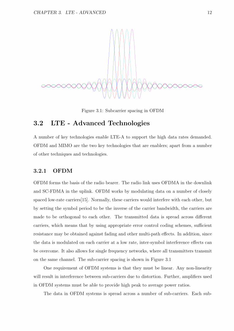
3.1 Subcarrier spacing in OFDM . . . . . . . . . . . . . . . . . . . . . . . . . . 12

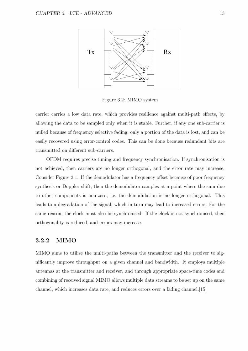
3.2 MIMO system . . . . . . . . . . . . . . . . . . . . . . . . . . . . . . . . . . 13

3.3 The LTE Protocol Stack . . . . . . . . . . . . . . . . . . . . . . . . . . . . 18

3.4 The LTE Type 1 Frame Structure . . . . . . . . . . . . . . . . . . . . . . . 18

3.5 The LTE Type 2 Frame Structure[2] . . . . . . . . . . . . . . . . . . . . . 19

3.6 Downlink Resource Grid[2] . . . . . . . . . . . . . . . . . . . . . . . . . . . 20

3.7 Overview of Physical Channel Processing[2] . . . . . . . . . . . . . . . . . 21

5.1 Percentage Packet Drops in Round Robin Scheduler . . . . . . . . . . . . . 29

5.2 Percentage Packet Drops in Opportunistic Scheduler . . . . . . . . . . . . 30

5.3 Percentage Packet Drops in Proportional Fair Scheduler . . . . . . . . . . . 31

5.4 Percentage Packet Drops in Proposed Modified Proportional Fair Scheduler 31

5.5 Comparison of PF With the Proposed Modified PF Scheduler in Terms of

Percentage Packet Drops . . . . . . . . . . . . . . . . . . . . . . . . . . . . 32

5.6 Percentage Packet Drops in Proposed Modified Opportunistic Scheduler . . 32

5.7 Comparison of Opportunistic With the Proposed Modified Opportunistic

Scheduler in Terms of Percentage Packet Drops . . . . . . . . . . . . . . . 33

5.8 Comparison of Proposed Modified Opportunistic Scheduler With the Pro-

posed Modified Proportional Fair Scheduler in Terms of Percentage Packet

Drops . . . . . . . . . . . . . . . . . . . . . . . . . . . . . . . . . . . . . . 34

v

List of Tables

3.1 Summary of relay classification & features in 3GPP rel. 10 . . . . . . . . . 17

3.2 Uplink-Downlink Configurations in Type 2 LTE Frame[2] . . . . . . . . . . 19

3.3 Physical Resource Block Parameters[2] . . . . . . . . . . . . . . . . . . . . 20

3.4 Modulation and Coding Schemes Used for Various CQI Indices[3] . . . . . 22

5.1 Values of β for all CQI[14] . . . . . . . . . . . . . . . . . . . . . . . . . . . 27

5.2 Parameters Used in the Simulation . . . . . . . . . . . . . . . . . . . . . . 28

vi

List of Abbreviations

ηx mean of x

σx standard deviation of x

2G 2nd generation

3G 3rd generation

3GPP 3rd Generation Partnership Project

4G 4th generation

CQI channel quality indicator

DwPTS downlink pilot time slot

E-ESM exponential-effective SINR mapping

eNB evolved node B

FDD frequency division duplexing

GP guard period

GPF generalised proportional fairness

JFI Jain’s fairness index

LoS line of sight

LTE Long Term Evolution

LTE-A Long Term Evolution - Advanced

vii

LIST OF TABLES viii

MIMO multiple-input multiple-output

MU-MIMO Multiple user multiple-input multiple-output

OFDM orthogonal frequency division multiplexing

OFDMA orthogonal frequency division multiple access

PDSCH physical downlink shared channel

PF proportional fair

QAM quadrature amplitude modulation

QoS quality of service

QPSK quadrature phase shift keying

SC-FDMA single carrier frequency division multiple access

SINR signal-to-interference-plus-noise ratio

SNR signal-to-noise ratio

STBC space-time block codes

TD-LTE Time Division - Long Term Evolution

TDD time division duplexing

TTL time to live

UE user equipment

UpPTS uplink pilot time slot

VoIP Voice over internet protocol

Chapter 1

Introduction

The past few years have seen a boom in cellular communications. In a span of a few years,

we have moved from 2G to 3G and are now in the process of deploying 4th generation

wireless communications. With every generation, we have seen architectural & technology

improvements which allow us to send more and more bits using the same wireless channel.

Not only is spectrum a rare and precious resource, the increasing traffic demands mean

that we have to use it more carefully than ever before.

Most of the technology standards specify various aspects of the physical layer, i.e.

the basic modulation and coding schemes essential for wireless transmission as well as

various protocols involved in the higher layers. However, the task of scheduling users for

quality-of-service (QoS) purposes has been left open, i.e. the service provider can decide

upon the implementation of scheduling algorithms to meet QoS requirements.

Each user has its own requirements, traffic model, and channel conditions. An ef-

ficient scheduling algorithm should provide users the quality-of-service they desire, with

guarantees on throughput, delay and fairness while making the best use of available re-

sources. Schedulers vary from very simple to very complex, and have been designed keep-

ing in consideration different measures for quality of service. The round-robin scheduler,

one of the simplest schedulers, was designed to schedule processes within an operating

system. It schedules processes one after another in a non-discriminatory fashion, making

it the most fair scheduler. On the other hand, the opportunistic scheduler designed for

wireless networks schedules the user with best channel conditions at any given instant.

This scheduler maximises the net system throughput, but can be very poor when fairness

1

CHAPTER 1. INTRODUCTION 2

is considered as a quality of service metric.

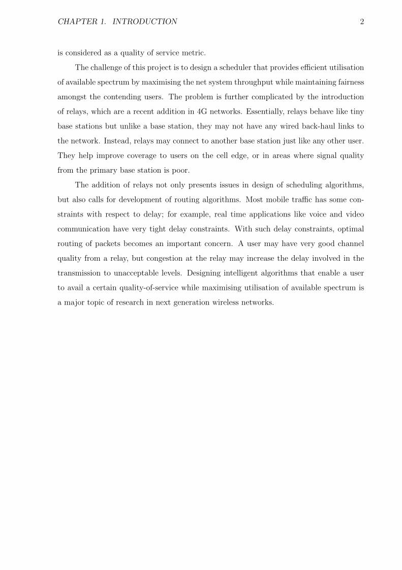
The challenge of this project is to design a scheduler that provides efficient utilisation

of available spectrum by maximising the net system throughput while maintaining fairness

amongst the contending users. The problem is further complicated by the introduction

of relays, which are a recent addition in 4G networks. Essentially, relays behave like tiny

base stations but unlike a base station, they may not have any wired back-haul links to

the network. Instead, relays may connect to another base station just like any other user.

They help improve coverage to users on the cell edge, or in areas where signal quality

from the primary base station is poor.

The addition of relays not only presents issues in design of scheduling algorithms,

but also calls for development of routing algorithms. Most mobile traffic has some con-

straints with respect to delay; for example, real time applications like voice and video

communication have very tight delay constraints. With such delay constraints, optimal

routing of packets becomes an important concern. A user may have very good channel

quality from a relay, but congestion at the relay may increase the delay involved in the

transmission to unacceptable levels. Designing intelligent algorithms that enable a user

to avail a certain quality-of-service while maximising utilisation of available spectrum is

a major topic of research in next generation wireless networks.

Chapter 2

Relay Architecture and Scheduling

Algorithms

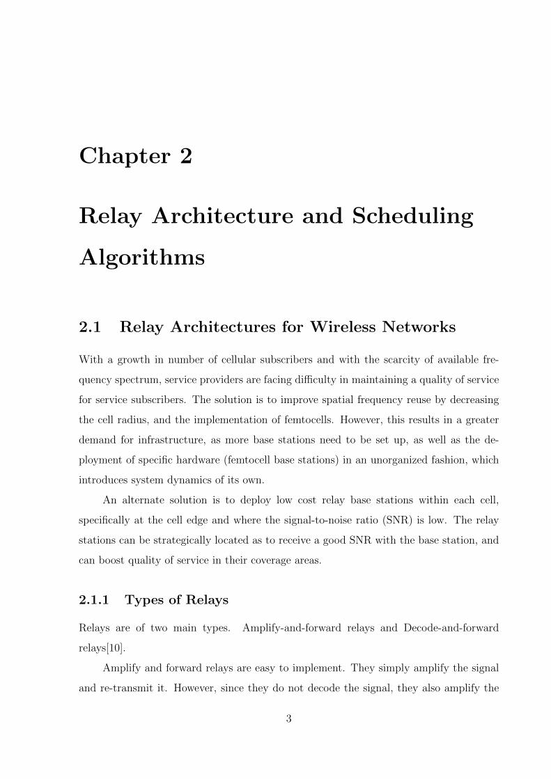
2.1 Relay Architectures for Wireless Networks

With a growth in number of cellular subscribers and with the scarcity of available fre-

quency spectrum, service providers are facing difficulty in maintaining a quality of service

for service subscribers. The solution is to improve spatial frequency reuse by decreasing

the cell radius, and the implementation of femtocells. However, this results in a greater

demand for infrastructure, as more base stations need to be set up, as well as the de-

ployment of specific hardware (femtocell base stations) in an unorganized fashion, which

introduces system dynamics of its own.

An alternate solution is to deploy low cost relay base stations within each cell,

specifically at the cell edge and where the signal-to-noise ratio (SNR) is low. The relay

stations can be strategically located as to receive a good SNR with the base station, and

can boost quality of service in their coverage areas.

2.1.1 Types of Relays

Relays are of two main types. Amplify-and-forward relays and Decode-and-forward

relays[10].

Amplify and forward relays are easy to implement. They simply amplify the signal

and re-transmit it. However, since they do not decode the signal, they also amplify the

3

CHAPTER 2. RELAY ARCHITECTURE AND SCHEDULING ALGORITHMS 4

degradation suffered by the signal, and do nothing to improve signal quality.

A decode and forward relay decodes the received information and re-encodes it before

forwarding a copy. Because of this process, the signal degradation is removed, and the

quality of service is improved. However, they are of high complexity because of the

presence of the decoder and encoder units.

Decode and forward relays have been further divided into two types.

Transparent Relays These relays do not communicate any control signals to the mo-

bile stations. Effectively, they overhear the mobile station’s transmission to the base

station, and forward a decoded and re-encoded copy to the base station when requested

to do so. So, the mobile station is not aware of the presence of transparent relays, and

the presence of transparent relays does not assist the mobile station in power control for

uplink transmissions.

Non-Transparent Relays Non-transparent relays communicate control signals with

the mobile stations. Effectively, they act as base stations for the mobile stations, and

have associated hand-over protocols, just as between base stations. The only difference

between the relay and the base station is that the relay does not have a backhaul network

for communication, but relies on a base station. Since the mobile station is aware of the

presence of the relay, it can control its power so as to minimize power loss in transmission,

while achieving better network coverage.

There are two major advantages of using relays in cellular networks. The first and

obvious advantage is to increase coverage. As relay stations are generally located closer to

the cell-edge, they can provide cell-edge users with improved service, thereby increasing

network coverage. The other advantage is that relays help improve the capacity of the

network. This is especially true in the case of OFDMA networks like LTE or WiMax;

the implementation of relays improves the received SINR by the users near the cell-edge,

which in turn reduces the number of resources allotted to each user. As the relay is

connected to the primary base station via a fairly good line-of-sight (LoS) link, the SNR

of the wireless link can be assumed to be sufficiently good. This allows more users to be

accommodated in the same spectrum, which increases network capacity.


2.2 Round Robin and Related Scheduling Algorithms

2.2.1 The Round Robin Scheduler

Round robin scheduling is extremely popular for scheduling processes on an operating

system. In an operating system, time slices are assigned to each process in equal portions

and in a circular order, without any priority. The round robin scheduler is simple, easy

to use and starvation free.

The round robin scheduler can also be used for data packet switching, as an alterna-

tive to the first-come-first-served queuing based scheduler. In this mechanism, separate

queues are maintained for every data-flow. The scheduler allows every data-flow which

has a non-empty queue to transmit a certain number of packets. This scheduling algo-

rithm works best when all packets are of equal length and achieves max-min fairness in

that case, i.e. the minimum data rates are maximized. If the packet size varies greatly

from one user to another, then the user with the larger packet size is favored, leading to

a loss in fairness.

The algorithm for the round robin scheduler is listed in Algorithm 1.

Algorithm 1 The Round Robin Scheduler

user being served← 0loopserve(user being served)user being served← user being served+ 1if user being served ≥ number of users thenuser being served← 0

end ifend loop

In a packet-based centralized wireless radio network with link-adaptation, the round-

robin algorithm is not optimal, as it assigns greater time to expensive users, with poor

channel conditions, if the same number of packets need to be transmitted. In such a

scenario, it makes more sense to wait until the channel conditions of a particular user

have improved before scheduling the user, in order to get better data rates, and hence

waste less time on an expensive user.


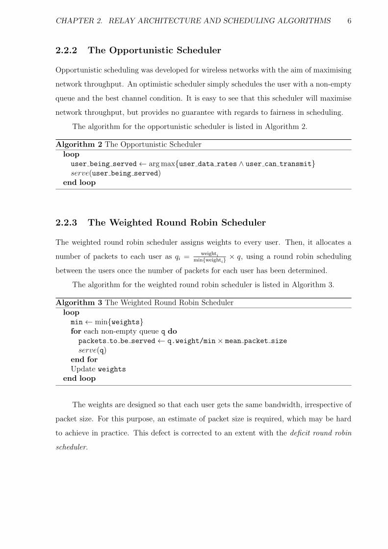
2.2.2 The Opportunistic Scheduler

Opportunistic scheduling was developed for wireless networks with the aim of maximising

network throughput. An optimistic scheduler simply schedules the user with a non-empty

queue and the best channel condition. It is easy to see that this scheduler will maximise

network throughput, but provides no guarantee with regards to fairness in scheduling.

The algorithm for the opportunistic scheduler is listed in Algorithm 2.

Algorithm 2 The Opportunistic Scheduler

loopuser being served← arg max{user data rates ∧ user can transmit}serve(user being served)

end loop

2.2.3 The Weighted Round Robin Scheduler

The weighted round robin scheduler assigns weights to every user. Then, it allocates a

number of packets to each user as qi = weightimin{weighti}

× q, using a round robin scheduling

between the users once the number of packets for each user has been determined.

The algorithm for the weighted round robin scheduler is listed in Algorithm 3.

Algorithm 3 The Weighted Round Robin Scheduler

loopmin← min{weights}for each non-empty queue q dopackets to be served← q.weight/min× mean packet size

serve(q)end forUpdate weights

end loop

The weights are designed so that each user gets the same bandwidth, irrespective of

packet size. For this purpose, an estimate of packet size is required, which may be hard

to achieve in practice. This defect is corrected to an extent with the deficit round robin

scheduler.


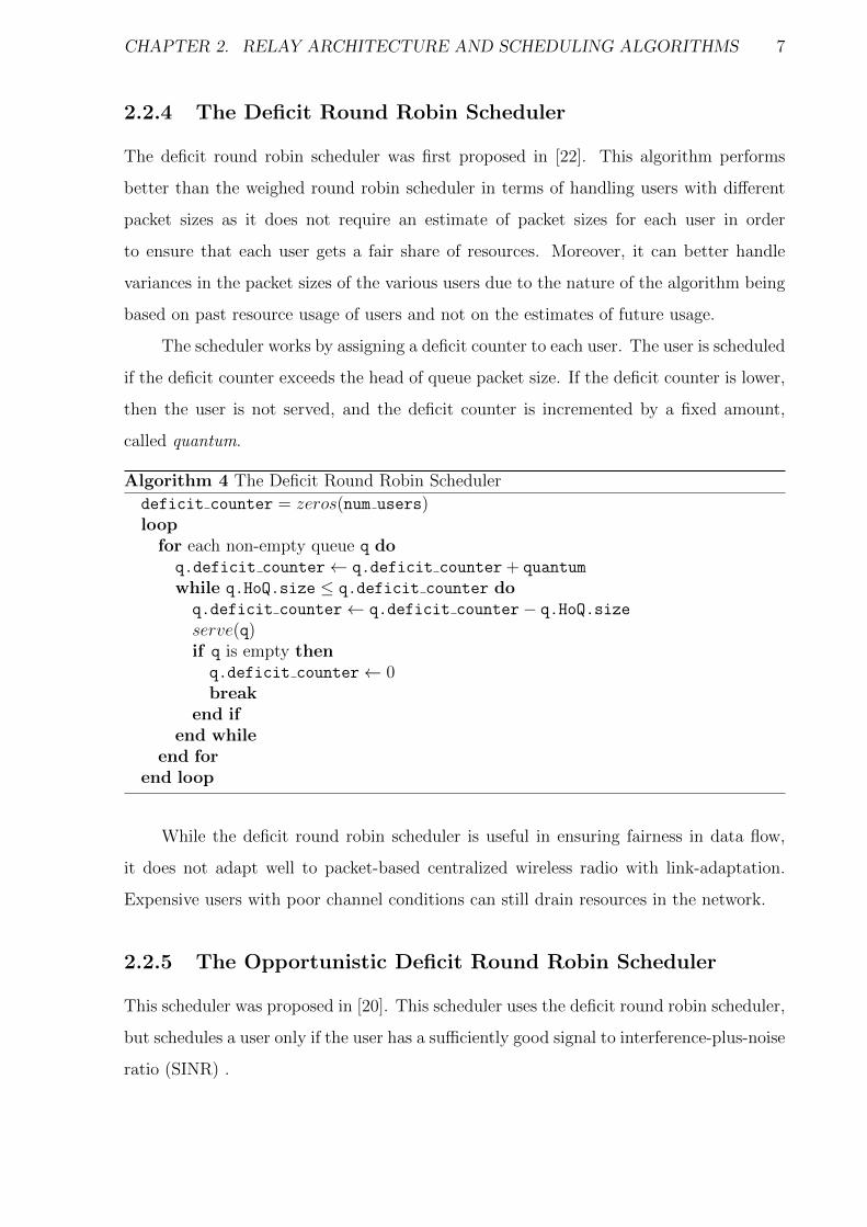
2.2.4 The Deficit Round Robin Scheduler

The deficit round robin scheduler was first proposed in [22]. This algorithm performs

better than the weighed round robin scheduler in terms of handling users with different

packet sizes as it does not require an estimate of packet sizes for each user in order

to ensure that each user gets a fair share of resources. Moreover, it can better handle

variances in the packet sizes of the various users due to the nature of the algorithm being

based on past resource usage of users and not on the estimates of future usage.

The scheduler works by assigning a deficit counter to each user. The user is scheduled

if the deficit counter exceeds the head of queue packet size. If the deficit counter is lower,

then the user is not served, and the deficit counter is incremented by a fixed amount,

called quantum.

Algorithm 4 The Deficit Round Robin Scheduler

deficit counter = zeros(num users)loop

for each non-empty queue q doq.deficit counter← q.deficit counter + quantum

while q.HoQ.size ≤ q.deficit counter doq.deficit counter← q.deficit counter− q.HoQ.size

serve(q)if q is empty thenq.deficit counter← 0break

end ifend while

end forend loop

While the deficit round robin scheduler is useful in ensuring fairness in data flow,

it does not adapt well to packet-based centralized wireless radio with link-adaptation.

Expensive users with poor channel conditions can still drain resources in the network.

2.2.5 The Opportunistic Deficit Round Robin Scheduler

This scheduler was proposed in [20]. This scheduler uses the deficit round robin scheduler,

but schedules a user only if the user has a sufficiently good signal to interference-plus-noise

ratio (SINR) .


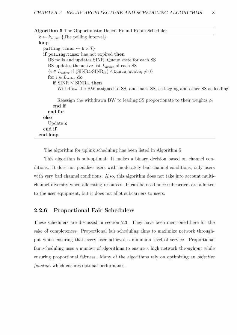
Algorithm 5 The Opportunistic Deficit Round Robin Scheduler

k← kinitial {The polling interval}looppolling timer← k× Tfif polling timer has not expired then

BS polls and updates SINR, Queue state for each SSBS updates the active list Lactive of each SS{i ∈ Lactive if (SINR>SINRth) ∧ Queue statei 6= 0}for i ∈ Lactive do

if SINR ≤ SINRth thenWithdraw the BW assigned to SSi and mark SSi as lagging and other SS as leading

Reassign the withdrawn BW to leading SS proportionate to their weights φiend if

end forelse

Update k

end ifend loop

The algorithm for uplink scheduling has been listed in Algorithm 5

This algorithm is sub-optimal. It makes a binary decision based on channel con-

ditions. It does not penalize users with moderately bad channel conditions, only users

with very bad channel conditions. Also, this algorithm does not take into account multi-

channel diversity when allocating resources. It can be used once subcarriers are allotted

to the user equipment, but it does not allot subcarriers to users.

2.2.6 Proportional Fair Schedulers

These schedulers are discussed in section 2.3. They have been mentioned here for the

sake of completeness. Proportional fair scheduling aims to maximize network through-

put while ensuring that every user achieves a minimum level of service. Proportional

fair scheduling uses a number of algorithms to ensure a high network throughput while

ensuring proportional fairness. Many of the algorithms rely on optimizing an objective

function which ensures optimal performance.


2.3 Fair Schedulers

An important parameter to be considered when analyzing schedulers is fairness. Depend-

ing on the nature of the system and the application involved, the notion of fairness varies.

Various approaches have been described to measure fairness[9, 7, 17, 19].

Jain’s fairness Index[9] is defined as

JFI =(∑u

i=1 xi)2

u∑u

i=1 x2i

(2.1)

where we have u users with xi is the amount of resource allotted to user i.

JFI is a number between 0 and 1; 0 being unfair and 1 being fair. While JFI can be

used as a reliable measure of fairness, we need to investigate the fairness in the transport

layer.

The TCP Fairness Index is defined as[17]

TFI =

(∑ui=1M

(ψiζi

))2

∑ui=1M

(ψiζi

)2 (2.2)

where

M(x) =

x if 0 ≤ x ≤ 1

1 otherwise

(2.3)

and ψi is the total throughput achieved by user i at the transport layer and ζi is the

throughput achieved by user i in a round robin scheduler. The TFI measures fairness in

comparison with a round robin scheduler.

Proportional Fairness A set of rates Ri is said to be proportionally fair if the Ris are

feasible and if, for every other feasible set of rates Si, the following holds[11]∑i

Si −Ri

Ri

≤ 0 (2.4)

A number of schedulers try to achieve proportional fairness[6, 13, 21], as it strikes

a balance between maximizing network throughput while ensuring that every user gets a

minimum level of fairness.

A simple algorithm for proportional fair scheduling is listed in Algorithm 6.


Algorithm 6 A Simple Proportional Fair Scheduler

loopfor each channel c do

for each user u dou.data rate(c)← (1−α)× u.data rate(c)+α× u.current data rate(c)

u.index← u.current data rate(c)u.data rate(c)

scheduled user = arg max{u.index}scheduled user.transmit(c)

end forend for

end loop

However, proportional fair schedulers may not maximize network throughput or

proportional fairness in multi-cell networks. This is because users in mobile networks

associate with the base station which offers best SNR. This algorithm does not balance

loads as to maximize throughput or fairness. A scheduler which takes into account the

entire network is described in [5]. The paper also describes a concept of generalised

proportional fairness (GPF), which takes the entire network into consideration, and not

just one cell.

Chapter 3

LTE - Advanced

LTE-Advanced represents the 4th generation in cellular wireless communication. This

technology was proposed by NTT DoCoMo of Japan, and was adopted by the ITU in

2009, and finalised by the 3GPP in March 2011. LTE represents a quantum leap in

cellular wireless communication because of specific features which take advantage of ad-

vance topology networks; optimized heterogeneous networks with a mix of macro-cells

and low power nodes such as femto-cells. LTE-Advanced further introduces multi-carriers

to improve performance in terms of ability to use ultra-wide bandwidth (up to 100 MHz).

3.1 Key Features in LTE - Advanced

Some of the main aims of LTE-A are listed below

• Peak data rates: 1 Gbps downlink, 500 Mbps uplink.

• Peak spectrum efficiency: 30 bps/Hz downlink, 15 bps/Hz uplink.

• Support for scalable bandwidth use and spectrum aggregation.

• LTE-A systems will be capable of inter-networking with LTE and 3GPP legacy

systems.

11

CHAPTER 3. LTE - ADVANCED 12

Figure 3.1: Subcarrier spacing in OFDM

3.2 LTE - Advanced Technologies

A number of key technologies enable LTE-A to support the high data rates demanded.

OFDM and MIMO are the two key technologies that are enablers; apart from a number

of other techniques and technologies.

3.2.1 OFDM

OFDM forms the basis of the radio bearer. The radio link uses OFDMA in the downlink

and SC-FDMA in the uplink. OFDM works by modulating data on a number of closely

spaced low-rate carriers[15]. Normally, these carriers would interfere with each other, but

by setting the symbol period to be the inverse of the carrier bandwidth, the carriers are

made to be orthogonal to each other. The transmitted data is spread across different

carriers, which means that by using appropriate error control coding schemes, sufficient

resistance may be obtained against fading and other multi-path effects. In addition, since

the data is modulated on each carrier at a low rate, inter-symbol interference effects can

be overcome. It also allows for single frequency networks, where all transmitters transmit

on the same channel. The sub-carrier spacing is shown in Figure 3.1

One requirement of OFDM systems is that they must be linear. Any non-linearity

will result in interference between sub-carriers due to distortion. Further, amplifiers used

in OFDM systems must be able to provide high peak to average power ratios.

The data in OFDM systems is spread across a number of sub-carriers. Each sub-


Figure 3.2: MIMO system

carrier carries a low data rate, which provides resilience against multi-path effects, by

allowing the data to be sampled only when it is stable. Further, if any one sub-carrier is

nulled because of frequency selective fading, only a portion of the data is lost, and can be

easily recovered using error-control codes. This can be done because redundant bits are

transmitted on different sub-carriers.

OFDM requires precise timing and frequency synchronisation. If synchronisation is

not achieved, then carriers are no longer orthogonal, and the error rate may increase.

Consider Figure 3.1. If the demodulator has a frequency offset because of poor frequency

synthesis or Doppler shift, then the demodulator samples at a point where the sum due

to other components is non-zero, i.e. the demodulation is no longer orthogonal. This

leads to a degradation of the signal, which in turn may lead to increased errors. For the

same reason, the clock must also be synchronised. If the clock is not synchronised, then

orthogonality is reduced, and errors may increase.

3.2.2 MIMO

MIMO aims to utilise the multi-paths between the transmitter and the receiver to sig-

nificantly improve throughput on a given channel and bandwidth. It employs multiple

antennas at the transmitter and receiver, and through appropriate space-time codes and

combining of received signal MIMO allows multiple data streams to be set up on the same

channel, which increases data rate, and reduces errors over a fading channel.[15]


Spatial diversity Spatial diversity often refers to transmit and receive diversity. This

provides resilience to fading by reducing the bit-error rate for a given SINR.

Spatial multiplexing Spatial multiplexing takes advantage of multiple paths to carry

additional traffic, i.e. it increases the data throughput capacity.

Because it uses multiple antennas, MIMO allows wireless technology to support

significantly higher data rates while still obeying Shannon’s law. By increasing the number

of transmit-receive pairs, we can linearly increase the traffic that can be supported in the

same bandwidth. This makes MIMO important for next generation wireless networks,

ans spectrum becomes an increasingly valuable commodity.

In order that MIMO systems can function, we need to apply appropriate coding

schemes so that the receiver may decode the data. This is done by applying a code not

just across time (which is the case for all communication systems) but also across the

various antennas. Such codes are called space-time codes.

Space-Time Codes

Space-time codes are used to enable transmission of multiple copies of a data stream using

multiple antennas and to exploit multiple copies of the received signal to combine them

in an optimal way to improve reliability of the communication link. Space-time coding

uses both spatial and temporal diversity.

When using space-time block coding, the data to be transmitted is divided into

blocks. Each block is then encoded by an appropriate space-time code, which can be

represented as a matrix as shown

Cmn =

s11 s12 · · · s1n

s21 s22 · · · s2n

......

. . ....

sm1 sm2 · · · smn

(3.1)

The resulting code is then transmitted by different antennas at different times. Each row

represents a time slot, and each column represents transmissions by a particular antenna

over time.


Alamouti Codes Alamouti codes, named after the developer, are an elegant way to

exploit transmit diversity without knowledge of channel conditions. It was developed for

exploiting diversity using two transmit antennas. The Alamouti code for two transmit

antennas[4] is denoted by the following matrix

C22 =

s1 s2

−s∗2 s∗1

(3.2)

Tarokh et al discovered a set of relatively straightforward higher order space-time

block codes[23, 24]. They proved that no code could achieve full rate for more than two

transmit antennas. While these codes have been improved upon, they serve as examples

of why the rate cannot reach 1; as well as other issues with producing good STBCs. A

linear decoding scheme which works under perfect channel state information assumption

was also discussed.

Differential Space-Time Block Codes Differential space-time block codes are a form

of code that does not require knowledge of channel impairments for decoding purposes.

These are generally based on standard space-time block codes, but transmit based on

differences in the input data blocks. This enables the receiver to extract data based on

the differences in the blocks in the set.

MU-MIMO Multiple User MIMO, or MU-MIMO is gaining popularity. It works by

scheduling multiple users to be able to access the same channel by utilising the spatial

degrees of freedom offered by MIMO.

3.3 Relays

Relaying is one of the features proposed for LTE-A systems. The aim of relaying is to

enhance coverage and capacity.

While the concept of relays is not new, and has been discussed in section 2.1, relays

in LTE are being considered to ensure optimal performance that meets the expectations

of users while keeping operational expenses within bounds.

While MIMO, OFDM and advanced error control techniques have helped increase

data rates in LTE, data rates are still poor near the cell-edge, where signal strength is the


lowest. As technology is being pushed to the limit, some alternate techniques are being

looked at to improve network performance. One such technique is to deploy relays near

the cell edge.

LTE relays are decode and forward relays. They demodulate the data, correct er-

rors, and re-transmit a new signal. The UE communicates with a relay, which in turns

communicates with a donor eNB. The relay is a fixed-infrastructure without a back-haul

connection and relays messages between a UE and an eNB through multi-hop transmis-

sions.

There are a number of advantages of using relays in LTE networks.

• Increased network density Relays can be easily deployed in situations where

network coverage must be increased by increasing number of base-stations. LTE

relays are easy to install and may be installed in convenient areas like lampposts,

walls, etc.

• Coverage in holes Relays can be deployed to fill coverage holes. Deploying a relay

near a coverage black-spot can help eliminate the coverage hole.

• Coverage outside main cell area Relays can also be used to extend coverage

beyond the primary cell area. This may be used for rapid network roll-out, and

eNBs can be installed later as traffic volumes increase.

LTE relays may operate in one of the following two modes[1]

• Half-duplex A half-duplex system provides communication in both directions, but

not simultaneously. The communication has to be multiplexed. In relay systems,

this means that the transmission has to be carefully scheduled. This can be either

static and pre-assigned, or dynamic and intelligent.

• Full-duplex A full-duplex relay can transmit and receive simultaneously. Often, in

LTE relays, this is done on the same frequency, but with a small delay (less than the

frame duration). In order to successfully operate relays in full-duplex mode, good

isolation between transmit and receive antennas is required.

Further, relays may be divided as


LTE RELAY CLASS CELL ID DUPLEX FORMAT

Type 1 Yes Inband half-duplex

Type 1a Yes Outband full-duplex

Type 1b Yes Inband full-duplex

Type 2 No Inband full-duplex

Table 3.1: Summary of relay classification & features in 3GPP rel. 10

• Inband The eNB—relay link operate on the same band as the eNB—UE link.

• Outband The eNB—relay link operates on a different band than the eNB—UE (or

relay—UE) link.

Type 1 LTE Relay Nodes Type 1 LTE relay nodes appear as base stations to the

UE. They have their own synchronisation and control signals, and provide backward

compatibility. Type 1 relay nodes are further divided in the following categories

• Type 1a These are full-duplex outband relays.

• Type 1b These are full-duplex inband relays.

Type 2 LTE Relay Nodes Type 2 LTE Relay nodes do not have their own identity,

and appear just like the primary eNB in a cell. A UE will not be able to distinguish a

type 2 relay node from the primary eNB in the cell.

The types of LTE relays are summarised in Table 3.1

3.4 Physical Layer

The LTE physical layer is defined in [2].

The fundamental unit of time in the LTE physical layer is Ts = 1/(15000× 2048)s.

All times are mentioned with respect to this unit of time.

Uplink and Downlink transmissions are organised into radio frames with Tf =

307200 × Ts = 10ms duration. Two radio frame structures are supported. Transmis-

sions in upto 4 secondary cells can be aggregated along with the primary cell. The UE

may assume that the same frame structure is being used in all 5 cells.


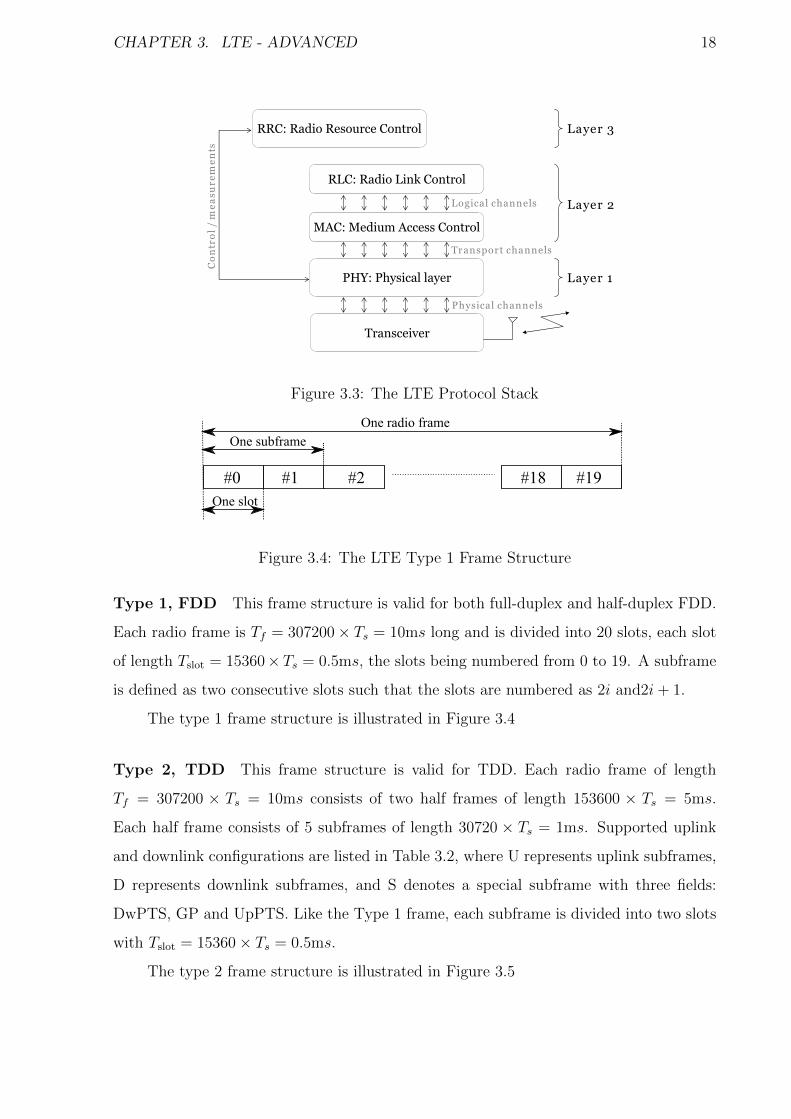
Figure 3.3: The LTE Protocol Stack

Figure 3.4: The LTE Type 1 Frame Structure

Type 1, FDD This frame structure is valid for both full-duplex and half-duplex FDD.

Each radio frame is Tf = 307200× Ts = 10ms long and is divided into 20 slots, each slot

of length Tslot = 15360× Ts = 0.5ms, the slots being numbered from 0 to 19. A subframe

is defined as two consecutive slots such that the slots are numbered as 2i and2i+ 1.

The type 1 frame structure is illustrated in Figure 3.4

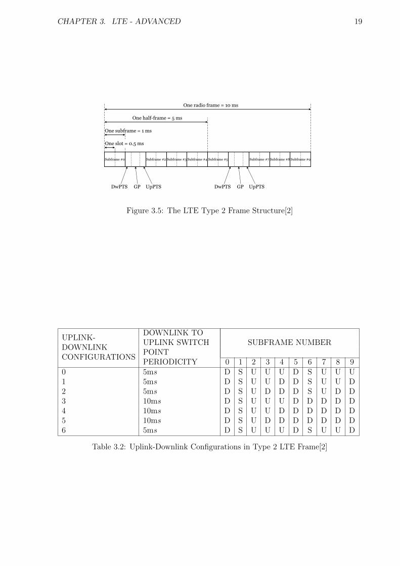
Type 2, TDD This frame structure is valid for TDD. Each radio frame of length

Tf = 307200 × Ts = 10ms consists of two half frames of length 153600 × Ts = 5ms.

Each half frame consists of 5 subframes of length 30720 × Ts = 1ms. Supported uplink

and downlink configurations are listed in Table 3.2, where U represents uplink subframes,

D represents downlink subframes, and S denotes a special subframe with three fields:

DwPTS, GP and UpPTS. Like the Type 1 frame, each subframe is divided into two slots

with Tslot = 15360× Ts = 0.5ms.

The type 2 frame structure is illustrated in Figure 3.5


Figure 3.5: The LTE Type 2 Frame Structure[2]

UPLINK-DOWNLINKCONFIGURATIONS

DOWNLINK TOUPLINK SWITCHPOINTPERIODICITY

SUBFRAME NUMBER

0 1 2 3 4 5 6 7 8 90 5ms D S U U U D S U U U1 5ms D S U U D D S U U D2 5ms D S U D D D S U D D3 10ms D S U U U D D D D D4 10ms D S U U D D D D D D5 10ms D S U D D D D D D D6 5ms D S U U U D S U U D

Table 3.2: Uplink-Downlink Configurations in Type 2 LTE Frame[2]


Figure 3.6: Downlink Resource Grid[2]

CONFIGURATION NRBsc NDL

symb

Normal cyclic prefix ∆f = 15kHz12

7

Extended cyclic prefix∆f = 15kHz 7

∆f = 7.5kHz 24 3

Table 3.3: Physical Resource Block Parameters[2]

3.5 Downlink

For the sake of brevity, this report describes only the downlink in LTE.

3.5.1 Slot Structure and Physical Resource Elements

The transmitted signal is described by one or several resource grids of NDLRBN

RBsc subcarriers

and NDLsymb OFDM symbols. The resource grid structure is illustrated in Figure 3.6. The

number of OFDM symbols in a slot depends on the cyclic prefix length and the subcarrier

spacing and is listed in Table 3.3


Figure 3.7: Overview of Physical Channel Processing[2]

Resource Blocks

Resource blocks are used to describe mapping of physical channels to resource elements.

A physical resource block is defined as NDLsymb consecutive OFDM symbols in the time

domain and NRBsc subcarriers in the frequency domain, where NDL

symb and NRBsc are defined

in Table 3.3. A physical resource block consists of NDLsymb×NRB

sc resource elements, which

corresponds to 180kHz in the frequency domain and one slot in the time domain.

General Structure For Downlink Physical Channels

The baseband signal representing a downlink physical channel is defined in terms of these

steps.

• Scrambling coded bits in each of the codewords to be transmitted.

• Modulation of scrambled bits to generate complex-valued modulation symbols.

• Mapping complex modulation symbols to one or more transmission layers.

• Precoding modulation symbols on each layer for transmission on antenna ports.

• Mapping complex modulation symbols for each antenna port to resource elements.

• Generation of complex-value time domain OFDM symbols for each antenna port.

These steps are illustrated in Figure 3.7 and are mentioned in [2].

3.5.2 Adaptive Modulation and Coding

LTE-A features adaptive modulation and coding based on the channel quality of the user.

The user communicates the channel quality via 4 bits reserved for indicating the channel


CQI INDEX MODULATION CODE RATE ×1024 EFFICIENCY0 N/A N/A N/A1 QPSK 78 0.15232 QPSK 120 0.23443 QPSK 193 0.37704 QPSK 308 0.60165 QPSK 449 0.87706 QPSK 602 1.17587 16QAM 378 1.47668 16QAM 490 1.91419 16QAM 616 2.406310 64QAM 466 2.730511 64QAM 567 3.322312 64QAM 666 3.902313 64QAM 772 4.523414 64QAM 873 5.115215 64QAM 948 5.5547

Table 3.4: Modulation and Coding Schemes Used for Various CQI Indices[3]

quality indicator (CQI) index, which serves as a basis for selecting a modulation and

coding scheme and consequently the data rate.

Channel Quality Indicator (CQI)

The CQI index is a 4 bit number ranging from 0 to 16. It serves as an indicator of the

channel quality and the basis of the selection of the modulation and coding scheme. The

CQI is defined in [3]. The UE reports the highest CQI index between 1 and 15 which

satisfies the condition that a single physical downlink shared channel (PDSCH) transport

block with a combination of modulation scheme and transport block size corresponding

to the CQI index, and occupying a group of downlink reference blocks termed the CSI

reference resource can be received with a transport block error probability not more than

10%.

The modulation and coding schemes employed for various CQI indices is listed in

Table 3.4

Chapter 4

Proposed Scheduling Algorithms

Two algorithms are proposed based on the existing opportunistic and proportional fair

algorithms. The modifications are motivated in order to reduce packet drops due to

deadline violation.

4.1 Modified Proportional Fair Scheduler

The disadvantage of the PF scheduling algorithm is that it does not take into account delay

constraints in scheduling decisions. To incorporate delay considerations in the scheduling

algorithm, a modification was proposed to the PF scheduler, which takes into account

the time-to-live (TTL) of the packet. An exponential penalty function is used to increase

priority of users which have packets with early deadlines. This function is illustrated in

Equation 4.1.

Φ1(TTL) = exp

(−TTL

t0

)(4.1)

Further, in an attempt to stabilise queue lengths, another penalty is added to increase the

index of users with longer queues. This penalty function is illustrated in Equation 4.2.

Φ2(q) = exp

(q

q0

)(4.2)

This penalty is multiplied with the PF index, and the resulting quantity is used as a

decision metric. The decision metric, or index, is listed in Equation 4.3.

PF index =r

r̄× Φ1(TTL)× Φ2(q) (4.3)

23

CHAPTER 4. PROPOSED SCHEDULING ALGORITHMS 24

where r is the instantaneous data rate of the user and r̄ is the average data rate computed

using an appropriate exponential weighting scheme.

The proposed algorithm has been listed in Algorithm 7.

Algorithm 7 Proposed modification to the proportional-fair scheduler


for each user u dou.data rate(c)← (1−α)× u.data rate(c)+α× u.current data rate(c)

u.index← u.current data rate(c)u.data rate(c)

× exp(−u.HoQ TTL

t0

)× exp

(u.queue length

q0

)scheduled user = arg max{u.index}scheduled user.transmit(c)

end forend for

end loop

4.2 Modified Opportunistic Scheduler

The necessity of the proportional fair algorithm in the presence of the additional penaltyterms is suspect. It was decided to check the performance of an opportunistic schedulerusing the same penalty functions mentioned in Equation 4.1 and Equation 4.2. The per-formance of the modified opportunistic scheduler is measured as against the performanceof the modified proportional fair algorithm.

The modified opportunistic scheduler uses an index mentioned in Equation 4.4

Opportunistic index = r × Φ1(TTL)× Φ2(q) (4.4)

The proposed modification to the opportunistic scheduler has been listed in Algorithm 8.

Algorithm 8 Proposed modification to the opportunistic scheduler


for each user u dou.index← u.current data rate(c)× exp

(−u.HoQ TTL

t0

)× exp

(u.queue length

q0

)scheduled user = arg max{u.index}scheduled user.transmit(c)

end forend for

end loop

Chapter 5

Simulation and Results

A system was created which would allow for easy system-level simulation for scheduling

exercises. The simulator was designed in C++, with an object-oriented approach which

would allow the simulator to be extended for any future work. A number of scheduling

algorithms were implemented on the system; in order to set benchmarks with regards

to system performance as well as to evaluate performance of proposed algorithms with

respect to the set benchmarks.

5.1 Simulation Setup

This section describes the simulation setup, with respect to the channel models used, the

cellular structure, and traffic models.

5.1.1 Logical channels

We consider logical channels with a bandwidth of 1.4 MHz each in 20 MHz of available

spectrum. This gives us 14 logical channels which can be allotted to users or relays. The

1.4 MHz allotted to a user is further divided into resource blocks as specified in the LTE

standards, each resource block occupying a 180 KHz bandwidth. This system allocates 7

resource blocks for each user, of which 6 are used in the downlink data communication,

and one resource block is used for feedback regarding channel quality[14].

25

CHAPTER 5. SIMULATION AND RESULTS 26

5.1.2 Placement of users

The simulation environment considers a seven-cell cluster like distribution of resources.

Users close to the base station are served by the base station, while users near the cell

edge are to be served by relays. For the purpose of scheduling, two logical channels

are allotted for users served by the primary base station, six channels are allotted for

communication between the base station and the 6 relays, and the remaining 6 channels

are allotted for the link between the relays and the users. However, it is important to note

that this allocation of channels is not a constraint, but is adopted just for simplifying the

scheduling algorithm design.

5.1.3 Channel Models

We attempt to simulate the system as a typical urban model. We consider path loss,

shadowing and fading effects.

Path loss effects are computed with an exponent of 3.5. We have considered i.i.d.

log-normal shadowing and i.i.d. Rayleigh fading in the channel model. The log-normal

shadowing changes slowly, after every 0.1s, while the Rayleigh fading changes with every

slot.

Hence, the SINR across each resource block is computed in the manner mentioned

in Equation 5.1.

SINR =Pt10ζλdγ∑6

i=1Pt10ζiλi

dγi+N0

(5.1)

where

Pt is the transmit power,

ζ is a normal random variable (log-normal shadowing),

λ is an exponential random variable (rayleigh fading),

γ is the path-loss exponent,

N0 is the thermal noise.

5.1.4 Traffic Models

The simulator allows for a number of traffic models. For the purpose of the simulation, we

assumed bursty traffic with identically sized packets of 500 bits each. The packets arrive


CQI VALUE β VALUE FOR E-ESM SINRthresh (dB)0 5 -∞1 5.01 -6.9342 5.01 -5.1473 0.84 -3.184 1.67 1.2545 1.61 0.7616 1.64 2.707 3.87 4.6978 5.06 6.5289 6.40 8.57610 12.59 10.3711 17.59 12.312 23.33 14.1813 29.45 15.8914 33.05 17.8215 35.41 19.83

Table 5.1: Values of β for all CQI[14]

with a Poisson burst rate of 0.4 packets for every slot. This rate was chosen so that the

network would be loaded to 70% of its capacity. At the same time, neighbouring cells are

assumed to have a random channel utilisation of 70%. Further, the time-to-live (TTL) of

the packets is changed, and scheduler performance is measured against the packet TTL.

5.1.5 Exponential-Effective SINR Mapping (E-ESM)

For the purpose of computing the CQI, it is necessary to know the SINR. It is possible

to calculate the SINR across each resource block, and then compute the block error

probability as a function of the SINRs, but such a function is almost impossible to derive

analytically. Instead, we use an effective SINR mapping method, which uses exponential

averaging to compute the effective SINR. This scheme is listed in Equation 5.2.

SINReff = −β ln

{1

N

N∑n=1

exp

(−SINRn

β

)}(5.2)

where β is a scaling factor which is tuned to optimise block error rate prediction. Such

optimal β are obtained numerically for different modulation and coding schemes.

[14] lists a table of β values corresponding to different CQI indices. The table is

reproduced in Table 5.1


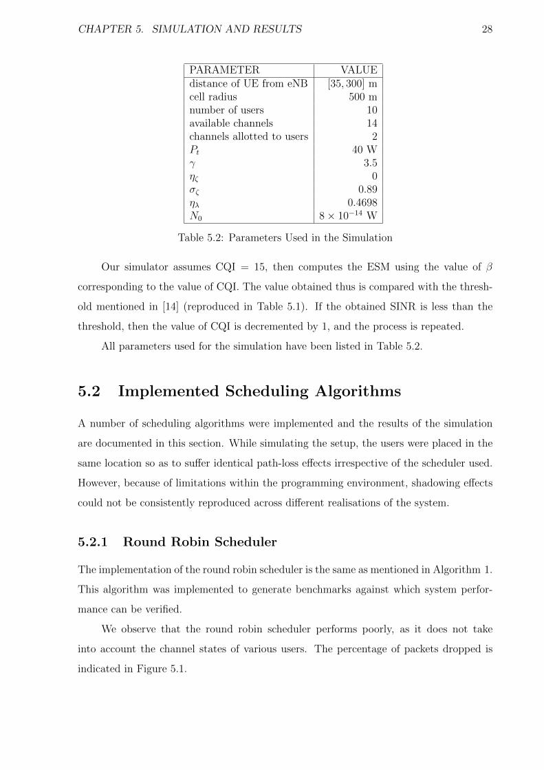
PARAMETER VALUEdistance of UE from eNB [35, 300] mcell radius 500 mnumber of users 10available channels 14channels allotted to users 2Pt 40 Wγ 3.5ηζ 0σζ 0.89ηλ 0.4698N0 8× 10−14 W

Table 5.2: Parameters Used in the Simulation

Our simulator assumes CQI = 15, then computes the ESM using the value of β

corresponding to the value of CQI. The value obtained thus is compared with the thresh-

old mentioned in [14] (reproduced in Table 5.1). If the obtained SINR is less than the

threshold, then the value of CQI is decremented by 1, and the process is repeated.

All parameters used for the simulation have been listed in Table 5.2.

5.2 Implemented Scheduling Algorithms

A number of scheduling algorithms were implemented and the results of the simulation

are documented in this section. While simulating the setup, the users were placed in the

same location so as to suffer identical path-loss effects irrespective of the scheduler used.

However, because of limitations within the programming environment, shadowing effects

could not be consistently reproduced across different realisations of the system.

5.2.1 Round Robin Scheduler

The implementation of the round robin scheduler is the same as mentioned in Algorithm 1.

This algorithm was implemented to generate benchmarks against which system perfor-

mance can be verified.

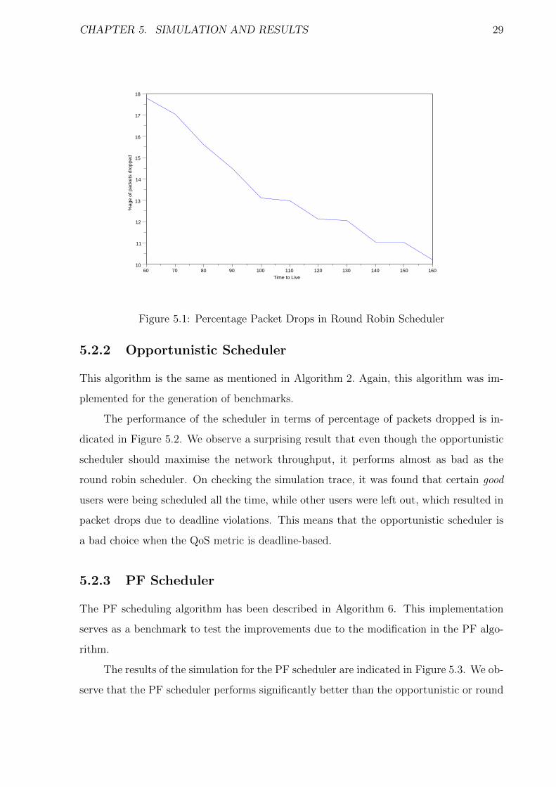
We observe that the round robin scheduler performs poorly, as it does not take

into account the channel states of various users. The percentage of packets dropped is

indicated in Figure 5.1.


10

11

12

13

14

15

16

17

18

60 70 80 90 100 110 120 130 140 150 160Time to Live

%ag

e of

pac

kets

dro

pped

Figure 5.1: Percentage Packet Drops in Round Robin Scheduler

5.2.2 Opportunistic Scheduler

This algorithm is the same as mentioned in Algorithm 2. Again, this algorithm was im-

plemented for the generation of benchmarks.

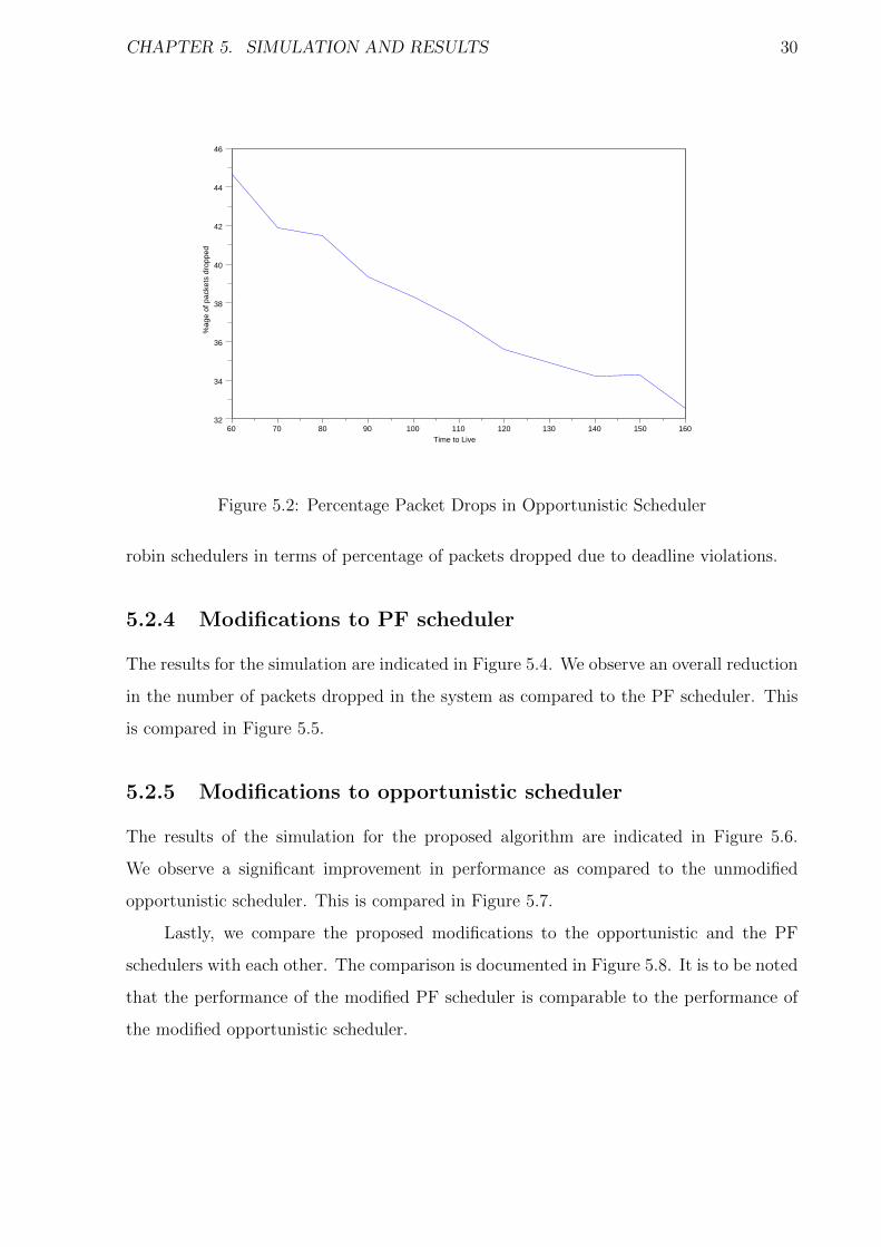
The performance of the scheduler in terms of percentage of packets dropped is in-

dicated in Figure 5.2. We observe a surprising result that even though the opportunistic

scheduler should maximise the network throughput, it performs almost as bad as the

round robin scheduler. On checking the simulation trace, it was found that certain good

users were being scheduled all the time, while other users were left out, which resulted in

packet drops due to deadline violations. This means that the opportunistic scheduler is

a bad choice when the QoS metric is deadline-based.

5.2.3 PF Scheduler

The PF scheduling algorithm has been described in Algorithm 6. This implementation

serves as a benchmark to test the improvements due to the modification in the PF algo-

rithm.

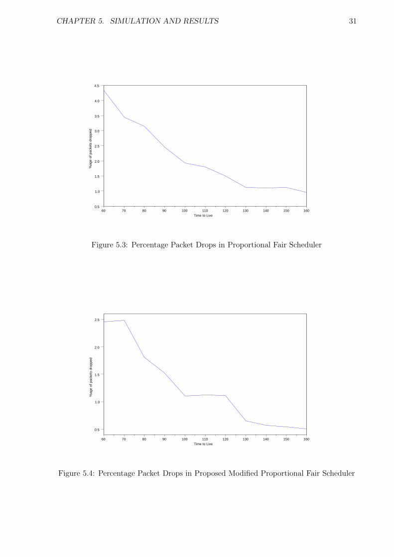
The results of the simulation for the PF scheduler are indicated in Figure 5.3. We ob-

serve that the PF scheduler performs significantly better than the opportunistic or round


32

34

36

38

40

42

44

46

60 70 80 90 100 110 120 130 140 150 160Time to Live

%ag

e of

pac

kets

dro

pped

Figure 5.2: Percentage Packet Drops in Opportunistic Scheduler

robin schedulers in terms of percentage of packets dropped due to deadline violations.

5.2.4 Modifications to PF scheduler

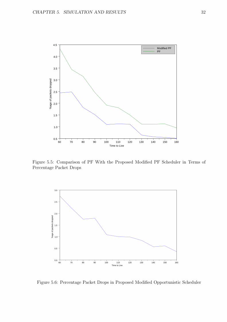
The results for the simulation are indicated in Figure 5.4. We observe an overall reduction

in the number of packets dropped in the system as compared to the PF scheduler. This

is compared in Figure 5.5.

5.2.5 Modifications to opportunistic scheduler

The results of the simulation for the proposed algorithm are indicated in Figure 5.6.

We observe a significant improvement in performance as compared to the unmodified

opportunistic scheduler. This is compared in Figure 5.7.

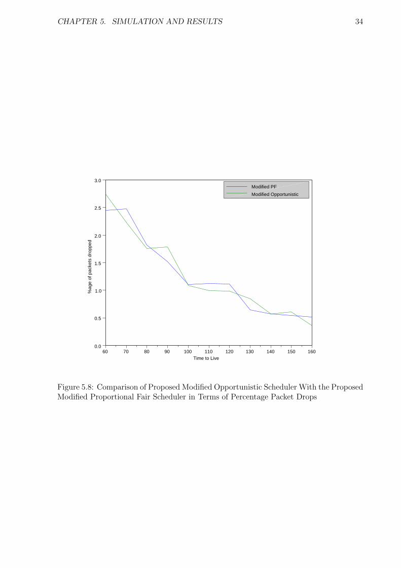
Lastly, we compare the proposed modifications to the opportunistic and the PF

schedulers with each other. The comparison is documented in Figure 5.8. It is to be noted

that the performance of the modified PF scheduler is comparable to the performance of

the modified opportunistic scheduler.


0.5

1.0

1.5

2.0

2.5

3.0

3.5

4.0

4.5

60 70 80 90 100 110 120 130 140 150 160Time to Live

%ag

e of

pac

kets

dro

pped

Figure 5.3: Percentage Packet Drops in Proportional Fair Scheduler

0.5

1.0

1.5

2.0

2.5

60 70 80 90 100 110 120 130 140 150 160Time to Live

%ag

e of

pac

kets

dro

pped

Figure 5.4: Percentage Packet Drops in Proposed Modified Proportional Fair Scheduler


Modified PFPF

0.5

1.0

1.5

2.0

2.5

3.0

3.5

4.0

4.5

60 70 80 90 100 110 120 130 140 150 160Time to Live

%ag

e of

pac

kets

dro

pped

Figure 5.5: Comparison of PF With the Proposed Modified PF Scheduler in Terms ofPercentage Packet Drops

0.0

0.5

1.0

1.5

2.0

2.5

3.0

60 70 80 90 100 110 120 130 140 150 160Time to Live

%ag

e of

pac

kets

dro

pped

Figure 5.6: Percentage Packet Drops in Proposed Modified Opportunistic Scheduler


Modified Opportunistic

Opportunistic

0

5

10

15

20

25

30

35

40

45

60 70 80 90 100 110 120 130 140 150 160Time to Live

%ag

e of

pac

kets

dro

pped

Figure 5.7: Comparison of Opportunistic With the Proposed Modified OpportunisticScheduler in Terms of Percentage Packet Drops


Modified PF

Modified Opportunistic

0.0

0.5

1.0

1.5

2.0

2.5

3.0

60 70 80 90 100 110 120 130 140 150 160Time to Live

%ag

e of

pac

kets

dro

pped

Figure 5.8: Comparison of Proposed Modified Opportunistic Scheduler With the ProposedModified Proportional Fair Scheduler in Terms of Percentage Packet Drops

Chapter 6

Conclusions and Future Work

The modifications to the opportunistic and the proportional fair schedulers are innovative

and simple to implement. At the same time, they help to a great extent in improving

the performance of the schedulers within the given QoS metrics of packet drops due to

deadline exhaustion.

A number of extensions and improvements to this project are possible.

Extension to relays The existing scheduler and simulation setup can be extended to

simulate relay-assisted networks. The algorithms mentioned here have to be modified

appropriately to adapt them to relay-assisted networks. One method which can be used

is delay apportioning which apportions the Time to Live between the eNB–relay and the

relay–UE links.

Better simulation of the LTE-A physical layer The simulation of the LTE-A phys-

ical layer in this model, while a good approximation, can be improved further to allow

for some of the more advanced features of LTE-A networks, like allowing for variable

bandwidth allocation to users, and simulation of MIMO systems.

Additional traffic models Currently, the simulator only has support for bursty traffic,

which does not completely model all the scenarios possible. The performance analysis of

the proposed schedulers must be studied for different models like broadband traffic[16],

VoIP, etc.

35

CHAPTER 6. CONCLUSIONS AND FUTURE WORK 36

Reinfocement learning based algorithms for scheduling and routing A possibil-

ity to be explored is the employment of a reinforcement learning algorithm to the problem

of dynamic resource block allocation, which would direct the way for self-organizing relays,

not unlike the power control in femtocell networks mentioned in [8]

Appendix A

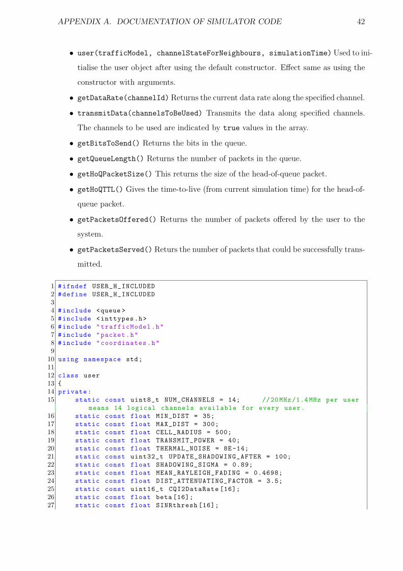
Documentation of Simulator Code

The code for the simulator is listed here.

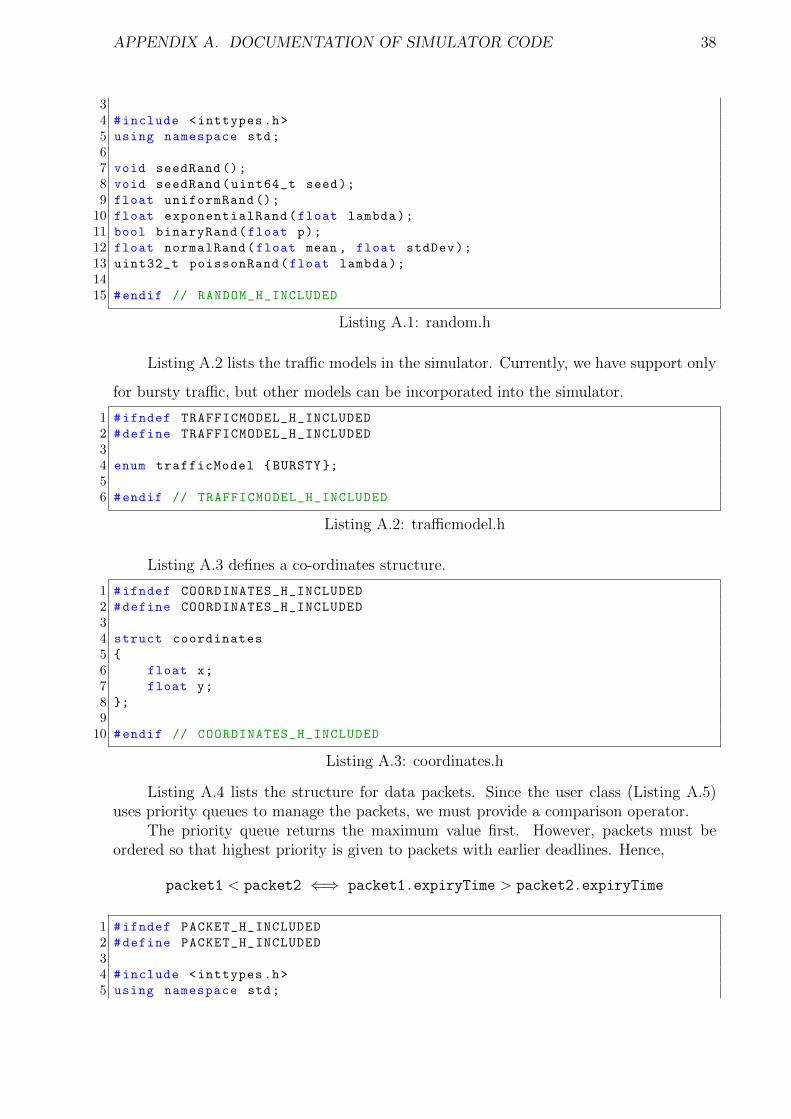
Listing A.1 lists the function prototypes for generating random numbers. It uses

the C++ random number generation library and improves it to provide random numbers

from a variety of distributions.

• seedRand(uint64 t seed) This function seeds the default C++ random number

generator. If a 64 bit seed value is provided, it seeds the random number generator

using the value provided; if not, it uses the system clock to seed the random number

generator with the number of seconds elapsed since midnight, 1st January, 1970.

• uniformRand() This function returns a uniform random number between 0 and 1.

• exponentialRand(float lambda) This function returns an exponential random

variable with parameter lambda. Note that the mean of the generated random

variable will be 1lambda

.

• binaryRand(float p) This returns a true value with probability p and a false

value with probability 1− p.

• normalRand(float mean, float stdDev) This function returns a normal random

variable with mean mean and standard deviation stdDev. It generates a random

number from two uniform random numbers using the Box-Muller transform[18].

• poissonRand(float lambda) This function generates a Poisson random variable

with parameter lambda. It generates the random number using Knuth’s algorithm[12].

1 #ifndef RANDOM_H_INCLUDED

2 #define RANDOM_H_INCLUDED

37

APPENDIX A. DOCUMENTATION OF SIMULATOR CODE 38

34 #include <inttypes.h>

5 using namespace std;

67 void seedRand ();

8 void seedRand(uint64_t seed);

9 float uniformRand ();

10 float exponentialRand(float lambda);

11 bool binaryRand(float p);

12 float normalRand(float mean , float stdDev);

13 uint32_t poissonRand(float lambda);

1415 #endif // RANDOM_H_INCLUDED

Listing A.1: random.h

Listing A.2 lists the traffic models in the simulator. Currently, we have support only

for bursty traffic, but other models can be incorporated into the simulator.

1 #ifndef TRAFFICMODEL_H_INCLUDED

2 #define TRAFFICMODEL_H_INCLUDED

34 enum trafficModel {BURSTY };

56 #endif // TRAFFICMODEL_H_INCLUDED

Listing A.2: trafficmodel.h

Listing A.3 defines a co-ordinates structure.

1 #ifndef COORDINATES_H_INCLUDED

2 #define COORDINATES_H_INCLUDED

34 struct coordinates

5 {

6 float x;

7 float y;

8 };

910 #endif // COORDINATES_H_INCLUDED

Listing A.3: coordinates.h

Listing A.4 lists the structure for data packets. Since the user class (Listing A.5)uses priority queues to manage the packets, we must provide a comparison operator.

The priority queue returns the maximum value first. However, packets must beordered so that highest priority is given to packets with earlier deadlines. Hence,

packet1 < packet2 ⇐⇒ packet1.expiryTime > packet2.expiryTime

1 #ifndef PACKET_H_INCLUDED

2 #define PACKET_H_INCLUDED




67 class packet

8 {

9 public:

10 uint16_t size;

11 uint32_t expiryTime;

1213 packet (): size (0), expiryTime (0) {}

14 bool operator < (const packet& pkt) const

15 {

16 return expiryTime > pkt.expiryTime; //This may appear

contradictory , but packets are placed in a priority queue.

Prority is higher for packets with an earlier deadline.

17 }

18 };

1920 #endif // PACKET_H_INCLUDED

Listing A.4: packet.h

Listing A.5 defines the main user class. The class has been organised into the fol-

lowing sections

Constants These are constants used in the simulation. Most of them are self-explanatory.

• MIN DIST is the minimum distance from the base station where users can be placed.

• MAX DIST is the maximum distance from the base stations where users can be placed.

This is less than the CELL RADIUS as the remaining users are to be supported by

relays.

• UPDATE SHADOWING AFTER specifies the number of slots after which the shadowing

should be updated. In order to save computing power, the simulator does not

compute channel state every slot, but only when requested by certain functions.

This behaviour has been documented in a later section.

• SHADOWING SIGMA specifies the standard deviation of the normal random variable

used to generate the log-normal fading. It specifies the standard deviation of ζ, and

the log-normal shadowing is computed as 10ζ .

• MEAN RAYLEIGH FADING specifies the mean of the exponential random variable used

to simulate the Rayleigh-fading channel. If the amplitude of the signal is Rayleigh

distributed, then the power is exponentially distributed. Hence, in computation of

SINR, an exponential random variable is multiplied to the transmit power.

• DIST ATTENUATING FACTOR specifies the path-loss exponent.


• CQI2DataRate, beta and SINRthresh are used in the E-ESM and CQI computation

used to calculate the data rate.

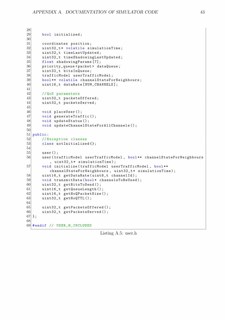
Variables These are private and not meant to be accessed directly.

• initialized This stores whether or not the class has been initialised correctly.

• position Stores the (x,y) co-ordinates of the user.

• simulationTime A pointer to simulation time. When the class is initialised, the

main programme must generate a variable scoped throughout the length of the

programme, and provide the user with a pointer to this variable. This serves as a

common clock to all users in the simulation.

• timeLastUpdated The simulation time instance when the object was refreshed.

Note that objects are not refreshed at every slot, but only when queried. This

speeds up simulation.

• timeShadowingLastUpdated The time the shadowing was last updated.

• shadowingParams This array stores the shadowing variables for the current cell, as

well as from the 6 neighbouring cells. It stores 10ζ , where ζ ∼ N (0, SHADOWING SIGMA).

• dataQueue The queue to hold packets. This is a priority queue, so the head-of-queue

packet is always the one which expires earliest.

• bitsInQueue The number of bits that have been stored in the queue. This is

different from the queue length, which is the number of packets in the queue.

• userTrafficModel The traffic model for the user. One of the traffic models listed

in Listing A.2. Currently, only bursty traffic is supported. However, support for

other models like VoIP, M/Pareto[16] and others can be added.

• channelStateForNeighbours A pointer to a 2-D array, which stores channel activ-

ity in neighbouring cells. The main programme must create this array, and provide

all users with a pointer to the array. Also, the main programme must update this

array at every slot instance before querying any users in that slot.

• dataRate Stores the possible data rate across each channel at the time instance

last queried. This is a hack to save simulation steps; by storing the data rate, the

E-ESM algorithm does not have to be invoked every time the user is queried.


• QoS Parameters packetsOffered and packetsServed store the number of pack-

ets offered and served to the users until the current instant of time. These are useful

in evaluating performance of scheduling algorithms in terms of packets dropped.

Private Member Functions These member functions are private, which means that

they cannot be accessed outside the class. They are used internally for some updates.

• placeUser() places the user uniformly inside the annulus defined by MIN DIST and

MAX DIST.

• generateTraffic() generates traffic for one slot using the specified traffic model.

• updateStatus() refreshes the status of the user to the current simulation time

instant. This includes refreshing the data rate, generating traffic until the current

time-slot and dropping packets whose deadlines have expired.

• updateChannelStateForAllChannels() computes data rates across all channels.

It is called by updateStatus().

Public Member Functions These provide handles to the user class to the end-user

of the simulation setup. The main programme must access the user class only via these

functions.

• notInitialized This is an exception class. When the main programme tries to

access a user object which has not been completely initialized, this error is thrown.

• user() The default constructor. It does not initialise the user object completely.

Instead, the resulting user object must be initialised using the initialize function.

• user(trafficModel, channelStateForNeighbours, simulationTime) The con-

structor. The main programme must provide the user with the three quantities; it

must define the traffic model to be used, and provide the user object with pointers

to the channel state for neighbours array, which indicates whether corresponding

channels in neighbouring cells are active; and the pointer to simulation time. This

constructor initialises the user object completely, and no further initialisation is

needed.


• user(trafficModel, channelStateForNeighbours, simulationTime) Used to ini-

tialise the user object after using the default constructor. Effect same as using the

constructor with arguments.

• getDataRate(channelId) Returns the current data rate along the specified channel.

• transmitData(channelsToBeUsed) Transmits the data along specified channels.

The channels to be used are indicated by true values in the array.

• getBitsToSend() Returns the bits in the queue.

• getQueueLength() Returns the number of packets in the queue.

• getHoQPacketSize() This returns the size of the head-of-queue packet.

• getHoQTTL() Gives the time-to-live (from current simulation time) for the head-of-

queue packet.

• getPacketsOffered() Returns the number of packets offered by the user to the

system.

• getPacketsServed() Returs the number of packets that could be successfully trans-

mitted.

1 #ifndef USER_H_INCLUDED

2 #define USER_H_INCLUDED

34 #include <queue >


6 #include "trafficModel.h"

7 #include "packet.h"

8 #include "coordinates.h"


1112 class user

13 {

14 private:

15 static const uint8_t NUM_CHANNELS = 14; //20MHz /1.4 MHz per user

means 14 logical channels available for every user.

16 static const float MIN_DIST = 35;

17 static const float MAX_DIST = 300;

18 static const float CELL_RADIUS = 500;

19 static const float TRANSMIT_POWER = 40;

20 static const float THERMAL_NOISE = 8E-14;

21 static const uint32_t UPDATE_SHADOWING_AFTER = 100;

22 static const float SHADOWING_SIGMA = 0.89;

23 static const float MEAN_RAYLEIGH_FADING = 0.4698;

24 static const float DIST_ATTENUATING_FACTOR = 3.5;

25 static const uint16_t CQI2DataRate [16];

26 static const float beta [16];

27 static const float SINRthresh [16];


2829 bool initialized;

3031 coordinates position;

32 uint32_t* volatile simulationTime;

33 uint32_t timeLastUpdated;

34 uint32_t timeShadowingLastUpdated;

35 float shadowingParams [7];

36 priority_queue <packet > dataQueue;

37 uint32_t bitsInQueue;

38 trafficModel userTrafficModel;

39 bool** volatile channelStateForNeighbours;

40 uint16_t dataRate[NUM_CHANNELS ];

4142 //QoS parameters

43 uint32_t packetsOffered;

44 uint32_t packetsServed;

4546 void placeUser ();

47 void generateTraffic ();

48 void updateStatus ();

49 void updateChannelStateForAllChannels ();

5051 public:

52 // Exception classes

53 class notInitialized {};

5455 user();

56 user(trafficModel userTrafficModel , bool** channelStateForNeighbours

, uint32_t* simulationTime);

57 void initialize(trafficModel userTrafficModel , bool**

channelStateForNeighbours , uint32_t* simulationTime);

58 uint16_t getDataRate(uint8_t channelId);

59 void transmitData(bool* channelsToBeUsed);

60 uint32_t getBitsToSend ();

61 uint16_t getQueueLength ();

62 uint16_t getHoQPacketSize ();

63 uint32_t getHoQTTL ();

6465 uint32_t getPacketsOffered ();

66 uint32_t getPacketsServed ();

67 };

6869 #endif // USER_H_INCLUDED

Listing A.5: user.h

Bibliography

[1] Further advancements for E-UTRA physical layer aspects. Technical Report 36.814,

3rd Generation Partnership Project, March 2010.

[2] Physical channels and modulation. Technical Report 36.211, 3rd Generation Part-

nership Project, December 2011.

[3] Physical layer procedures. Technical Report 36.213, 3rd Generation Partnership

Project, December 2011.

[4] S. M. Alamouti. A simple transmit diversity technique for wireless communications.

IEEE Journal on Selected Areas in Communications, 16(8):1451–1458, October 1998.

[5] T. Bu, L. Li, and R. Ramjee. Generalized proportional fair scheduling in third

generation wireless data networks. In Proceedings of the 25th IEEE International

Conference on Computer Communications, pages 1–12, April 2006.

[6] S. Deb, V. Mhatre, and V. Ramaiyan. WiMAX relay networks: opportunistic

scheduling to exploit multiuser diversity and frequency selectivity. In Proceedings

of the 14th ACM international conference on Mobile computing and networking, Mo-

biCom ’08, pages 163–174, New York, NY, USA, 2008. ACM.

[7] M. Dianati, X. Shen, and S. Naik. A new fairness index for radio resource allocation

in wireless networks. In IEEE Wireless Communications and Networking Conference,

volume 2, pages 712–717, March 2005.

[8] A. Galindo-Serrano and L. Giupponi. Distributed Q-learning for interference control

in OFDMA-based femtocell networks. In VTC Spring, pages 1–5, 2010.

44

BIBLIOGRAPHY 45

[9] R. K. Jain, D.-M. W. Chiu, and W. R. Hawe. A Quantitative Measure Of Fairness

And Discrimination For Resource Allocation In Shared Computer Systems. Technical

report, Digital Equipment Corporation, September 1984.

[10] G. Joshi. On relay-assisted cellular networks. Master’s thesis, Indian Institute of

Technology, Bombay, June 2010.

[11] F. P. Kelly, A. K. Maulloo, and D. K. H. Tan. Rate control for communication

networks: Shadow prices, proportional fairness and stability. Journal of the Operation

Research Society, 49(3):237–252, March 1998.

[12] D. E. Knuth. The Art of Computer Programming, volume 2. Addison Wesley, 1969.

[13] R. Kwan, C. Leung, and J. Zhang. Proportional fair multiuser scheduling in LTE.

Signal Processing Letters, IEEE, 16(6):461–464, June 2009.

[14] X. Li, Q. Fang, and L. Shi. A effective SINR link to system mapping method for CQI

feedback in TD-LTE system. In IEEE 2nd International Conference on Computing,

Control and Industrial Engineering, volume 2, pages 208–211, August 2011.

[15] U. Madhow. Fundamentals of Digital Communication. Cambridge University Press,

2008.

[16] T. D. Neame, M. Zuckerman, and R. G. Addie. Modelling broadband traffic streams.

In Global Telecommunications Conference, volume 1B, pages 1048–1052, December

1999.

[17] K. Norlund, T. Ottosson, and A. Brunstrom. TCP fairness measures for scheduling

algorithms in wireless networks. In 2nd International Conference on Quality of Service

in Heterogeneous Wired/Wireless Networks, pages 8–20, August 2005.

[18] A. Papoulis and S. Pillai. Probability, Random Variables And Stochastic Processes.

Tata McGraw-Hill Education, 2002.

[19] H. Rath. On Channel and Transport Layer Aware Scheduling and Congestion Control

in Wireless Networks. PhD thesis, Indian Institute of Technology, Bombay, July 2009.

BIBLIOGRAPHY 46

[20] H. Rath and A. Karandikar. An opportunistic-DRR (ODRR) uplink scheduling

scheme for IEEE 802.16-based wireless networks. In IETE International Conference

on Next Generation Networks, February 2006.

[21] M. Salem, A. Adinoyi, M. Rahman, H. Yanikomeroglu, D. Falconer, and Y.-D. Kim.

Fairness-aware radio resource management in downlink OFDMA cellular relay net-

works. IEEE Transactions on Wireless Communications, 9(5):1628–1639, May 2010.

[22] M. Shreedhar and G. Varghese. Efficient fair queueing using deficit round robin.

SIGCOMM Computer Communication Review, 25:231–242, October 1995.

[23] V. Tarokh, H. Jafarkhani, and A. Calderbank. Space-time block codes from orthogo-

nal designs. IEEE Transactions on Information Theory, 45(5):1456–1467, July 1999.

[24] V. Tarokh, H. Jafarkhani, and A. Calderbank. Space-time block coding for wireless

communications: performance results. IEEE Journal on Selected Areas in Commu-

nications, 17(3):451–460, March 1999.