Download pdf - Convergence and Consistency Analysis for Extended Kalman Filter Based SLAM

1036 IEEE TRANSACTIONS ON ROBOTICS, VOL. 23, NO. 5, OCTOBER 2007

Convergence and Consistency Analysis forExtended Kalman Filter Based SLAM

Shoudong Huang, Member, IEEE, and Gamini Dissanayake, Member, IEEE

Abstract—This paper investigates the convergence propertiesand consistency of Extended Kalman Filter (EKF) based simul-taneous localization and mapping (SLAM) algorithms. Proofsof convergence are provided for the nonlinear two-dimensionalSLAM problem with point landmarks observed using a range-and-bearing sensor. It is shown that the robot orientation uncertaintyat the instant when landmarks are first observed has a significanteffect on the limit and/or the lower bound of the uncertainties ofthe landmark position estimates. This paper also provides someinsights to the inconsistencies of EKF based SLAM that have beenrecently observed. The fundamental cause of EKF SLAM incon-sistency for two basic scenarios are clearly stated and associatedtheoretical proofs are provided.

Index Terms—Convergence, extended information filter, ex-tended Kalman filter, inconsistency, simultaneous localization andmapping (SLAM).

I. INTRODUCTION

SIMULTANEOUS Localization and Mapping (SLAM) is theprocess of building a map of an environment while concur-

rently generating an estimate for the pose of the robot. Manydifferent techniques have been developed to solve the SLAMproblem (see [1] and the references therein). However, the useof an Extended Kalman Filter (EKF) to estimate a state vectorcontaining both the robot pose (including position and orienta-tion) and the landmark locations (e.g., [2]) remains one of themost popular strategies for solving SLAM.

While there have been numerous implementations, only veryfew analytical results on the convergence and essential proper-ties of the EKF SLAM algorithm are available. Dissanayake et al.provided convergence properties of SLAM and lower bound onthepositionuncertainty [2].These resultswereextendedto multi-robots SLAM in [3]. Kim [4] provided some further analysis onthe asymptotic behavior for the onedimensional SLAMproblem.All the proofs presented in the literature ([2]–[6]), however, onlydeals with simple linear formulations of the SLAM problem.

Almost all practical SLAM implementations need to dealwith nonlinear process and observation models. The results due

Manuscript received April 5, 2006; revised November 12, 2006. This paperwas recommended for publication by Associate Editor W. Burgard and EditorL. Parker upon evaluation of the reviewers’ comments. This work was supportedby the ARC Centre of Excellence program, funded by the Australian ResearchCouncil (ARC) and the New South Wales State Government. This paper waspresented in part at 2006 IEEE International Conference on Robotics and Au-tomation, Orlando, FL, May 15–19, 2006.

The authors are with the ARC Centre of Excellence for Autonomous Sys-tems, Faculty of Engineering, University of Technology, Sydney, NSW 2007,Australia (e-mail: [email protected]; [email protected]).

Color versions of one or more of the figures in this paper are available onlineat http://ieeexplore.ieee.org.

Digital Object Identifier 10.1109/TRO.2007.903811

to [2] are intuitive and many early experiments and computersimulations appear to confirm that the properties of the linearsolution extends to practical nonlinear problems. In the pastfew years, a number of researchers have demonstrated that thelower bound for the map accuracy presented in [2] is violatedand the EKF SLAM produces inconsistent estimates due toerrors introduced during the linearization process [7], [8], [9],[10], [11]. While some explanation of this phenomena has beenreported, mainly through Monte Carlo simulations, a thoroughtheoretical analysis of the nonlinear SLAM problem is not yetavailable.

This paper provides both the key convergence proper-ties and the explicit formulas for the covariance matricesfor some basic scenarios in the nonlinear two-dimensionalEKF SLAM problem with point landmarks observed using arange-and-bearing sensor. Some insights to, and theoreticalproofs of the EKF SLAM inconsistencies are also given. Theresults in this paper demonstrate that:

• Most of the convergence properties in [2] are still true forthe nonlinear case provided that the Jacobians used in theEKF equations are evaluated at the true states.

• The main reasons for inconsistency in EKF SLAM are dueto (i) the violation of some fundamental constraints gov-erning the relationship between various Jacobians whenthey are evaluated at the current state estimate, and (ii)the use of relative location information from robot to land-marks to update the absolute robot and landmark locationestimates.

• The robot orientation uncertainty plays an important rolein both the EKF SLAM convergence and the possible in-consistency. In the limit, the inconsistency of EKF SLAMmay cause the variance of the robot orientation estimate tobe incorrectly reduced to zero.

The paper is organized as follows. In Section II, the EKFSLAM algorithm is restated in a form more suitable for theoret-ical analysis. In Section III, some key convergence propertiesare proved. The theoretical explanations of the EKF SLAMinconsistency are given in Section IV. Section V providessome discussions on related work and further research topics.Section VI concludes the paper. Most of the proofs and relevantbackground material are given in the Appendices.1

II. RESTATEMENT OF THE EKF SLAM ALGORITHM

In this section, the EKF SLAM algorithm is restated usingslightly different notations and formulas in order to clearly stateand prove the results in this paper.

1Details of the proofs omitted due to space constraints are available from thefirst author.

1552-3098/$25.00 © 2007 IEEE

HUANG AND DISSANAYAKE: CONVERGENCE AND CONSISTENCY ANALYSIS FOR EXTENDED KALMAN FILTER BASED SLAM 1037

A. State Vector in 2-D EKF SLAM

The state vector is denoted as2

(1)

where is the robot orientation, is the robotposition, are the positionsof the point-landmarks. Note that the robot orientation isseparated from the robot position because it plays a crucial rolein the convergence and consistency analysis.

B. Prediction

1) Process Model: The robot process model considered inthis paper is

and is denoted as

(2)

where are the “controls”, are zero-mean Gaussiannoise on . is the time interval of one movement step. Theexplicit formula of function depends on the particular robot.Two examples of this general model are given below.

2) Example 1: A simple discrete-time robot motion model

(3)

which can be obtained from a direct discretization of the uni-cycle model (e.g., [10])

(4)

where is the velocity and is the turning rate.3) Example 2: A car-like vehicle model (e.g., [2])

(5)

where is the velocity and is the steering angle, is thewheel-base of the vehicle.

2To simplify the notation, the vector transpose operator is omitted. For ex-ample, X;X ;X ; . . . ; X are all column vectors and the rigorous notationshould be X = (�;X ;X ; . . . ;X ) .

The process model of landmarks (assumed stationary) is

(6)

Thus, the process model of the whole system is

(7)

where is the function combining (2) and (6).4) Prediction: Suppose at time , after the update, the esti-

mate of the state vector is

and the covariance matrix of the estimation error is . Theprediction step is given by

(8)

where is the covariance of the control noise , andare given by3

(9)

Here and are Jacobians of in (2) with respect tothe robot pose and the control noise , respec-tively, evaluated at the current estimate .

For the system described by (2), the Jacobian with respect tothe robot pose is

(10)

The Jacobian with respect to the controls, , depends onthe detailed formula of function in (2).

C. Update

1) Measurement Model: At time , the measurement ofth landmark, obtained using sensor on board the robot, is given

by range and bearing

(11)

where and are the noise on the measurements.The observation model can be written in the general form

(12)

The noise is assumed to be Gaussian with zero-mean andcovariance matrix .

3In this paper, I and 0 always denote the identity matrix and a zero matrixwith an appropriate dimension, respectively.


2) Update: Equation to update the covariance matrix can bewritten in the information form ([12]) as follows:

(13)

where is the information matrix, is the new informa-tion obtained from the observation given by

(14)

and is the Jacobian of function evaluated at the currentestimate .

The estimate of the state vector can now be updated using

(15)

where

(16)

and

(17)

Remark 2.1: Using (13), (14) and the matrix inversion lemma[see (99) in Appendix B]

(18)

which is the typical EKF update formula.The Jacobian of the measurement function is

(19)

where

(20)

Note that, in the above, all the columns corresponding to land-marks that are not currently being observed have been ignored.

III. CONVERGENCE PROPERTIES OF EKF SLAM

This section proves some convergence results for 2-D non-linear EKF SLAM. The first result is the monotonically de-creasing property which is the same as Theorem 1 in [2].

Theorem 3.1: The determinant of any submatrix of the mapcovariance matrix decreases monotonically as successive obser-vations are made.

Proof: This result can be proved in a similar way to that ofTheorem 1 in [2]. The only difference is that the Jacobians in-

stead of the state transition matrix and observation matrices willbe used in the proof. The key point of the proof is “In the predic-tion step, the covariance matrix of the map does not change; inthe update step, the whole covariance matrix is nonincreasing.”The details of the proof are omitted.

For 2-D nonlinear EKF SLAM, general expressions for thecovariance matrices evolution cannot be obtained. Therefore,two basic scenarios are considered in the following: 1) the robotis stationary and observes new landmarks many times, and 2) therobot then moves but only observes the same landmarks.

Suppose the robot starts at point A, the initial uncertainty ofthe robot pose is expressed by the covariance matrix

(21)

where is a scalar and is a 2 2 matrix.The initial information matrix is denoted as

(22)

A. Scenario 1—Robot Stationary

Consider the scenario that the robot is stationary at point Aand makes observations.

1) Observe One Landmark: First assume that the robot canonly observe one new landmark – landmark . The Jacobian in(19) evaluated at the true landmark position and thetrue robot position is denoted as4

(23)

where

(24)

with

(25)

For convenience, further denote that

(26)

where denotes 2 2 identity matrix (see footnote 3).Theorem 3.2: If the robot is stationary and observes a new

landmark times, the covariance matrix of the robot pose andthe new landmark position estimates is

(27)

4For the theoretical convergence results, the Jacobians are always evaluated atthe true states. In the real SLAM applications, the Jacobians have to be evaluatedat the estimated states and this may cause inconsistency. A detailed analysis ofthis is given in Section IV.


where is the initial robot uncertainty given in (21), is de-fined in (24), is defined in (26), and is the observationnoise covariance matrix. In the limit when , the covari-ance matrix becomes

(28)

Proof: See Appendix A.The following corollary can be obtained from Theorem 3.2.Corollary 3.3: If the robot is stationary and observes a new

landmark times, the robot uncertainty remains unchanged.The limit (lower bound) on the covariance matrix of the newlandmark is

(29)

which is determined by the robot uncertainty and the Jaco-bian . In the special case when the initial uncertainty ofthe robot orientation is 0, is equal to the initial robotposition uncertainty in (21).

Proof: See Appendix A.Remark 3.4: Theorem 3.2 and Corollary 3.3 can be regarded

as the nonlinear version of Theorem 3 in [2]. Moreover, it is clearthat the robot orientation uncertainty has a significant effect onthe limit of the landmark uncertainty. “When the robot positionis exactly known but its orientation is uncertain, even if thereis a perfect knowledge about the relative location between thelandmark and the robot, it is still impossible to tell exactly wherethe true landmark position is.”

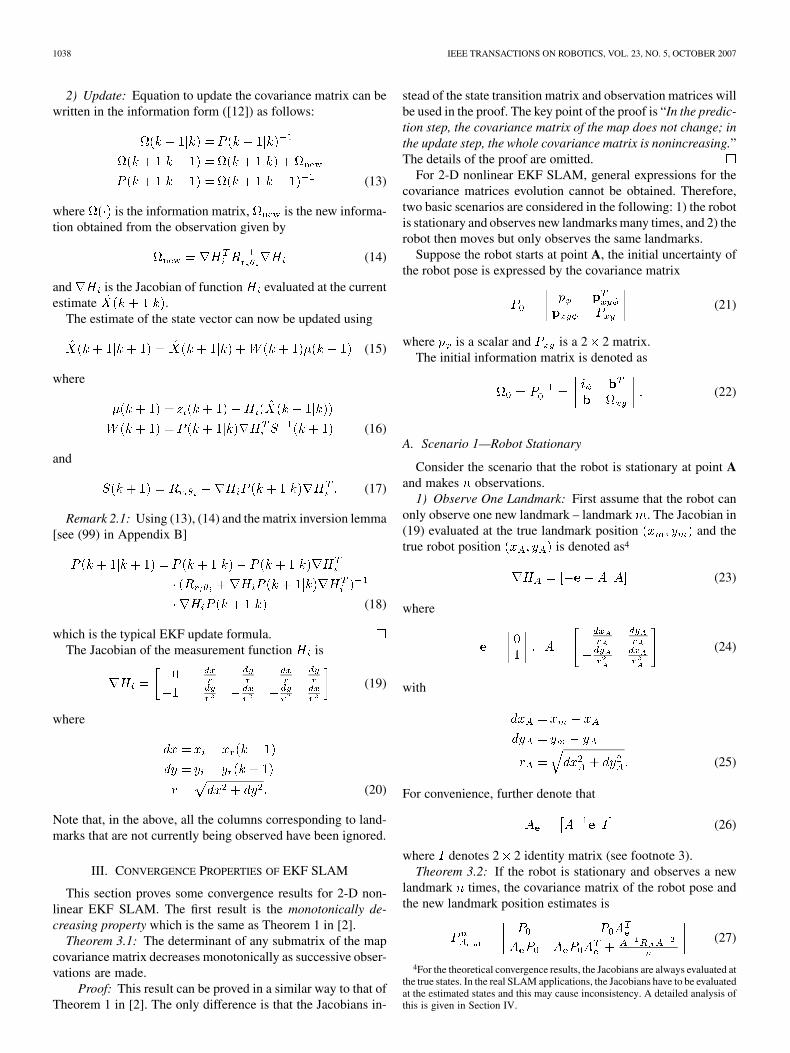
Fig. 1(a) and (b) show that the initial robot orientation uncer-tainty has a significant effect on the landmark estimation accu-racy. In Fig. 1(a), the initial uncertainty of the robot pose is

. Because the robot orientation uncertainty islarge (the standard deviation is 0.1732 radians degrees), inthe limit, the uncertainty of the landmark position is much largerthan the initial uncertainty of the robot position. In Fig. 1(b),the initial robot pose uncertainty is . Be-cause the robot orientation uncertainty is very small (the stan-dard deviation is 0.0316 radians degrees), in the limit, theuncertainty of the landmark position is very close to the initialuncertainty of the robot position.

2) Observe Two Landmarks: Suppose the robot can observetwo new landmarks (landmark and landmark ) at point A,then the dimension of the observation function in (12) is four(two ranges and two bearings), the Jacobian can be denoted as

(30)

where is similar to in (24) but defined for landmark .Similar to (26), denote

(31)

The following theorem and corollary can now be obtained.The proofs are similar to that of Theorem 3.2 and Corollary 3.3and are omitted here.

Theorem 3.5: If the robot is stationary and observes two newlandmarks times, the covariance matrix of the robot pose andthe two new landmark position estimates is

(32)

where

(33)

and is the observation noise covariance matrix for observinglandmark . In the limit when , the whole covariancematrix is

(34)

Corollary 3.6: If the robot is stationary and observes two newlandmarks times, the robot uncertainty remains unchanged.The limit (lower bound) of the covariance matrix associatedwith the two new landmarks is

(35)

In the special case when the initial uncertainty of the robot ori-

entation , the limit .

Remark 3.7: Theorem 3.5 and Corollary 3.6 are the analogueof Theorem 2 in [2]. However, because ,

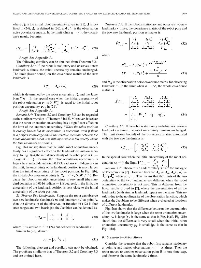
when . This means that the limits of the un-certainties of the two landmarks are different when the robotorientation uncertainty is not zero. This is different from thelinear results proved in [2], where the uncertainties of all thelandmarks (with similar landmark types) are the same. This re-sult is due to the nonlinearity of the observation function, whichmakes the Jacobians to be different when evaluated at locationsof different landmarks.

Fig. 2(a) shows that the difference between the uncertaintiesof the two landmarks is large when the robot orientation uncer-tainty is large [ is the same as that in Fig. 1(a)]. Fig. 2(b)shows that the difference is very small when the initial robotorientation uncertainty is small [ is the same as that inFig. 1(b)].

B. Scenario 2—Robot Moves

Consider the scenario that the robot first remains stationaryat point A and makes observations times. Then therobot moves to another observation point B in one time step,and observes the same landmarks times.


Fig. 1. Limits of landmark uncertainty when the robot is stationary and observes the landmark n ! 1 times (see Theorem 3.2, Corollary 3.3, and Theorem4.1): In Fig. 1(a) and (c), the initial uncertainty of the robot pose is P = diag(0:03; 1; 1). In Fig. 1(b) and (d), the initial robot pose uncertainty is P =diag(0:001;1; 1). For Fig. 1(a) and (b), the Jacobians are evaluated at the true robot and landmark locations. In Fig. 1(c) and (d), the solid ellipses are the limitof the uncertainties when the Jacobians are evaluated at the updated state estimate at each update step. (a) Initial robot orientation uncertainty is large. (b) Initialrobot orientation uncertainty is small. (c) Inconsistency of EKF SLAM. (d) Inconsistency can be neglected when initial robot orientation uncertainty is small.

1) Observe One Landmark: First assume that the robot canonly observe one new landmark (at points A and B) – landmark

. The Jacobian in (19) evaluated at point B and the true posi-tion of landmark is denoted as

(36)

where is similar to in (24) but defined for the robot pose atpoint B. Similar to (26), denote

(37)

The following lemma gives the relationship between the Ja-cobians at point A and point B.

Lemma 3.8: The relationship between the Jacobians atpoint A and point B is

(38)

where is the Jacobian of in (2) with respect to the robotorientation and position [see (10)], evaluated at the robot pose Aand the associated control values.

Proof: See Appendix A.The relationship given in Lemma 3.8 plays an important role

in deriving the following convergence results. Furthermore, it

will be shown in Theorem 4.2 in Section IV that the violationof this relationship may cause inconsistency in EKF SLAM.

Theorem 3.9: If the robot first remains stationary at point Aand observes one new landmark times before it movesto point B and observes the same landmark times, then the finalcovariance matrix is

(39)

where

(40)

(41)

with

(42)

and

(43)


Fig. 2. Limits of the two landmark uncertainties when the robot is stationary and makes observation n ! 1 times: Fig. 2(a) shows that the final uncertaintiesof the two landmarks are different. See Theorem 3.5, Corollary 3.6, Remark 3.7, Theorem 4.1, and the caption of Fig. 1 for more explanations. (a) Initial robotorientation uncertainty is large. (b) Initial robot orientation uncertainty is small. (c) Inconsistency of EKF SLAM for two landmarks. (d) Inconsistency can beneglected when initial robot orientation uncertainty is small.

Furthermore, if the matrix is invertible,5 then thematrix when . Here is defined in (28),

is the covariance matrix of the observation noise at point B,and are Jacobians of function in (2) evaluated

at point A and the associated control values.Proof: See Appendix A.

By Theorem 3.9, the lower bound of the covariance matrixis , which is the covariance matrix when the robot firstreaches point B if there is no control noise in moving from A toB [ in (8)].

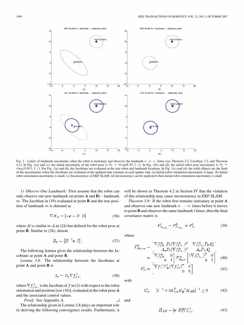
Fig. 3(a)–(d) illustrate Theorem 3.9. The initial robot uncer-tainty is the same as that used for Fig. 1(a). Fig. 3(a) and (b)show the case when there is no control noise. Fig. 3(a) showsthe uncertainties after the prediction step and Fig. 3(b) showsthe uncertainties after the update using the observations at pointB. It can be seen that the observations at point B cannot reducethe uncertainty of the robot and landmarks. Fig. 3(c) and (d)show the case when control noise is present. In this case, thelandmark uncertainty cannot be improved by the observation atpoint B, while the uncertainty of the robot can be reduced to thesame level as the case when there is no control noise. The limitsof the uncertainties are independent of the extent of sensor andcontrol noises. The control noise only affect the robot uncer-tainty after the prediction in Fig. 3(c). The sensor noise used are

5This depends on the process model and the direction of the robot movementbut this is true in most of the cases.

the same as those in Fig. 1, the robot speed and the control noises[in Fig. 3(c) and (d)] are deliberately enlarged, just to make thedifferences of the ellipses visible.

2) Observe Two Landmarks: Suppose the robot can observetwo new landmarks (landmark and landmark ) at points Aand B, then the dimension of the observation function in (12) isfour (two ranges and two bearings), denote the correspondingJacobians as given in (30) and

(44)

Theorem 3.10: If the robot first remains stationary at point Aand observes two new landmarks times before it movesto point B and observes the same two landmarks times, thenthe final covariance matrix is

(45)

where

(46)


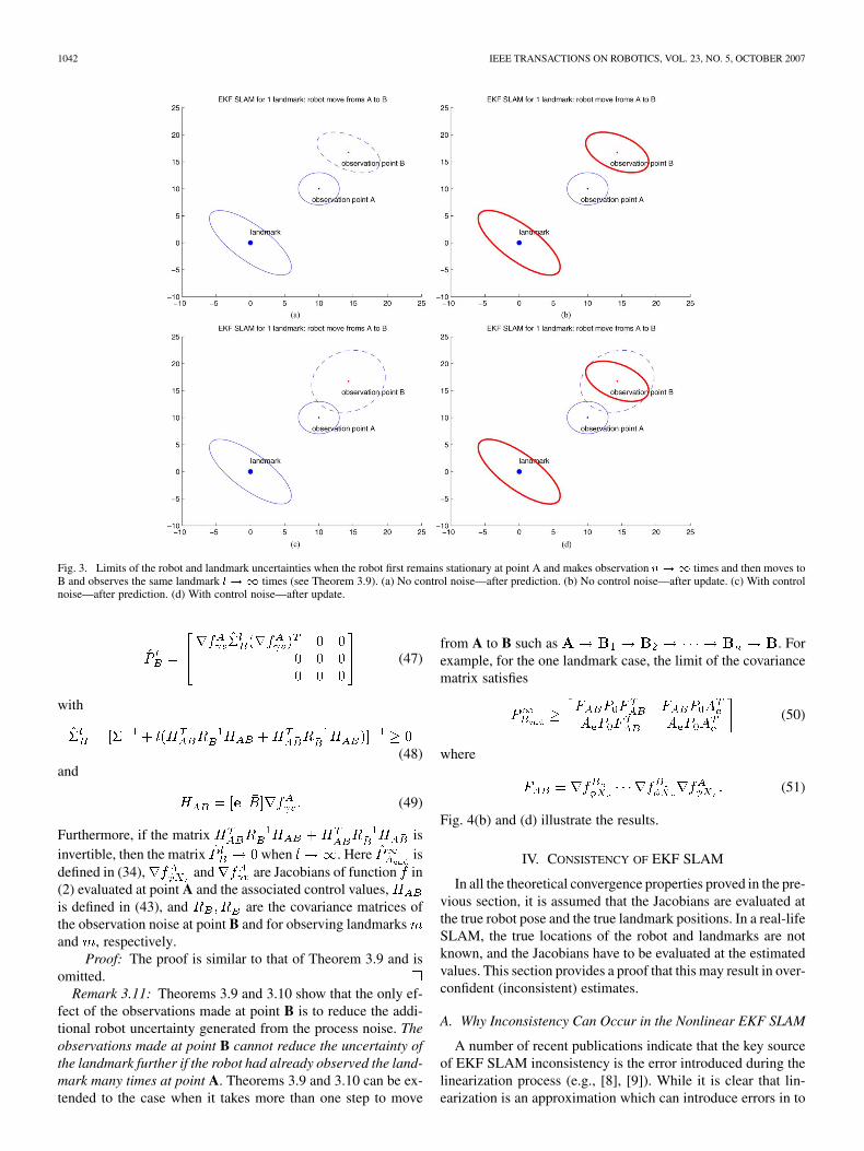
Fig. 3. Limits of the robot and landmark uncertainties when the robot first remains stationary at point A and makes observation n!1 times and then moves toB and observes the same landmark l ! 1 times (see Theorem 3.9). (a) No control noise—after prediction. (b) No control noise—after update. (c) With controlnoise—after prediction. (d) With control noise—after update.

(47)

with

(48)and

(49)

Furthermore, if the matrix isinvertible, then the matrix when . Here isdefined in (34), and are Jacobians of function in(2) evaluated at point A and the associated control values,is defined in (43), and are the covariance matrices ofthe observation noise at point B and for observing landmarksand , respectively.

Proof: The proof is similar to that of Theorem 3.9 and isomitted.

Remark 3.11: Theorems 3.9 and 3.10 show that the only ef-fect of the observations made at point B is to reduce the addi-tional robot uncertainty generated from the process noise. Theobservations made at point B cannot reduce the uncertainty ofthe landmark further if the robot had already observed the land-mark many times at point A. Theorems 3.9 and 3.10 can be ex-tended to the case when it takes more than one step to move

from A to B such as . Forexample, for the one landmark case, the limit of the covariancematrix satisfies

(50)

where

(51)

Fig. 4(b) and (d) illustrate the results.

IV. CONSISTENCY OF EKF SLAM

In all the theoretical convergence properties proved in the pre-vious section, it is assumed that the Jacobians are evaluated atthe true robot pose and the true landmark positions. In a real-lifeSLAM, the true locations of the robot and landmarks are notknown, and the Jacobians have to be evaluated at the estimatedvalues. This section provides a proof that this may result in over-confident (inconsistent) estimates.

A. Why Inconsistency Can Occur in the Nonlinear EKF SLAM

A number of recent publications indicate that the key sourceof EKF SLAM inconsistency is the error introduced during thelinearization process (e.g., [8], [9]). While it is clear that lin-earization is an approximation which can introduce errors in to


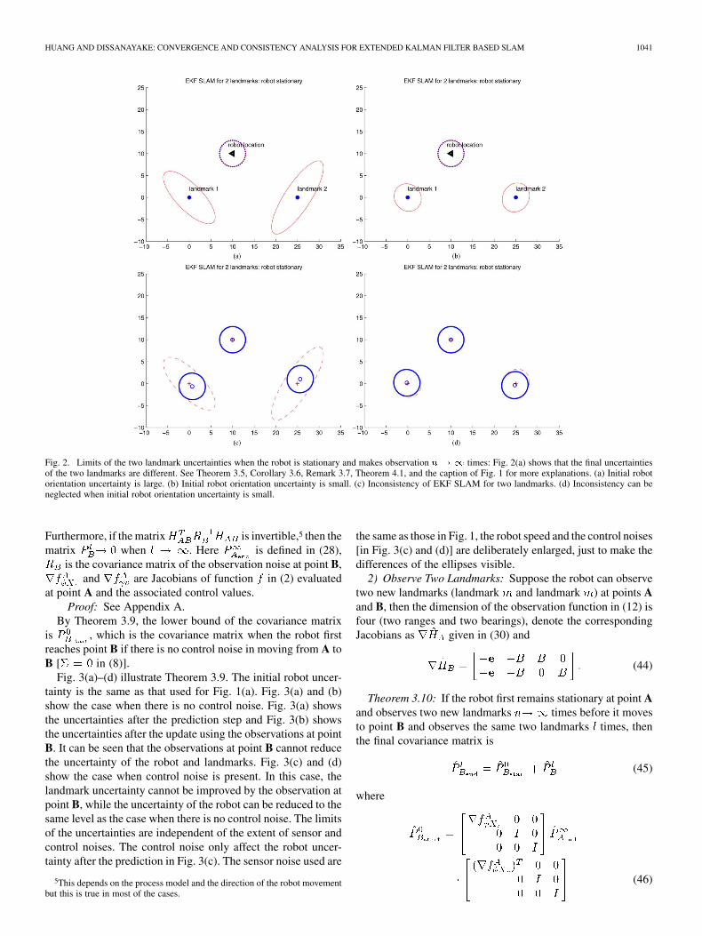
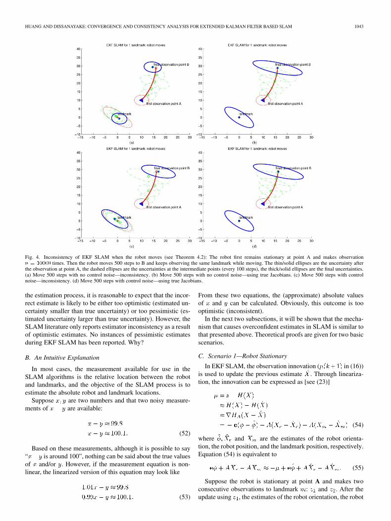
Fig. 4. Inconsistency of EKF SLAM when the robot moves (see Theorem 4.2): The robot first remains stationary at point A and makes observationn = 10000 times. Then the robot moves 500 steps to B and keeps observing the same landmark while moving. The thin/solid ellipses are the uncertainty afterthe observation at point A, the dashed ellipses are the uncertainties at the intermediate points (every 100 steps), the thick/solid ellipses are the final uncertainties.(a) Move 500 steps with no control noise—inconsistency. (b) Move 500 steps with no control noise—using true Jacobians. (c) Move 500 steps with controlnoise—inconsistency. (d) Move 500 steps with control noise—using true Jacobians.

the estimation process, it is reasonable to expect that the incor-rect estimate is likely to be either too optimistic (estimated un-certainty smaller than true uncertainty) or too pessimistic (es-timated uncertainty larger than true uncertainty). However, theSLAM literature only reports estimator inconsistency as a resultof optimistic estimates. No instances of pessimistic estimatesduring EKF SLAM has been reported. Why?

B. An Intuitive Explanation

In most cases, the measurement available for use in theSLAM algorithms is the relative location between the robotand landmarks, and the objective of the SLAM process is toestimate the absolute robot and landmark locations.

Suppose are two numbers and that two noisy measure-ments of are available:

(52)

Based on these measurements, although it is possible to say“ is around 100”, nothing can be said about the true valuesof and/or . However, if the measurement equation is non-linear, the linearized version of this equation may look like

(53)

From these two equations, the (approximate) absolute valuesof and can be calculated. Obviously, this outcome is toooptimistic (inconsistent).

In the next two subsections, it will be shown that the mecha-nism that causes overconfident estimates in SLAM is similar tothat presented above. Theoretical proofs are given for two basicscenarios.

C. Scenario 1—Robot Stationary

In EKF SLAM, the observation innovation ( in (16))is used to update the previous estimate . Through lineariza-tion, the innovation can be expressed as [see (23)]

(54)

where and are the estimates of the robot orienta-tion, the robot position, and the landmark position, respectively.Equation (54) is equivalent to

(55)

Suppose the robot is stationary at point A and makes twoconsecutive observations to landmark : and . After theupdate using , the estimates of the robot orientation, the robot


position, and the landmark position will change fromto , thus the Jacobian will be evaluated at a differentpoint in the state space when is used for the next update. Thetwo innovations give

(56)

where are defined in a manner similar to (24) butcomputed at the estimated robot and landmark locations. Both

are nonsingular matrices that are different but closeto .

The above two equations are equivalent to

(57)

So

(58)

By the special structure of [see (24)], if , thenand (58) provides some information on the value

of . It is obvious that observing a single new landmark will notimprove the knowledge of the robot orientation. Therefore, thisapparent information on the robot orientation is incorrect andwill result in overconfident estimates (inconsistency).

To examine the extent of the possible inconsistency, let therobot be stationary at point A and observe a new landmarktimes. Let the estimate be updated after each observation usingJacobians evaluated at the updated estimate at each time step.Denote the different Jacobians as

(59)

Let denote the observation noise covariance matrix at pointA, and define

(60)

As before, suppose that the initial robot uncertainty is givenby (21).

Theorem 4.1: In EKF SLAM, if the robot is stationary atpoint A and observes a new landmark times, the inconsistencyoccurs due to the fact that Jacobians are evaluated at differentstate estimates. The level of inconsistency is determined by theinitial robot uncertainty and the defined in (60).When , the inconsistency may cause the variance ofthe robot orientation estimate to be reduced to zero.

Proof: See Appendix A.Figs. 1(c), (d)–2(c), (d) illustrate the results in Theorem 4.1.

In Fig. 1(c), the initial uncertainty of the robot pose is the sameas that used in Fig. 1(a), the solid ellipse is the limit of the

landmark uncertainty when the Jacobian is evaluated at the up-dated state estimate at each update step. This figure is gener-ated by performing 1000 updates assuming that the range andbearing measurements are corrupted by random Gaussian noise(the standard deviations of range and bearing noise are selectedto be similar to that of a typical indoor laser scanner, 0.1 mand 1 , respectively). It can be seen that the uncertainty of thelandmark is reduced far below the theoretical limit (dashed el-lipse), demonstrating the inconsistency of EKF SLAM solution.In Fig. 1(d), the initial uncertainty of the robot orientation ismuch smaller [the same as that used in Fig. 1(b)]. It can be seenthat the extent of inconsistency is too small to be seen (the solidellipse almost coincides with the dashed one).

D. Scenario 2—Robot Moves

Consider the scenario that the robot observes a new landmarkat point A and then moves to point B and makes an observa-tion of the same landmark. Similar to (57), the two innovations

give

(61)

From the process model (2) with appropriate linearization

(62)

Thus

(63)

If , then the above equa-

tion contains information on , which is clearly incorrect asobservations to a single landmark do not provide any knowl-edge about the robot orientation.

Note that is actually the

relationship proved in Lemma 3.8. Therefore, the following re-sult can now be stated.

Theorem 4.2: When the robot observes the same landmarkat two different points A and B, the EKF SLAM algorithm mayprovide inconsistent estimates due to the fact that the Jacobiansevaluated at the estimated robot positions may violate the keyrelationship between the Jacobians as shown in Lemma 3.8.

Proof: See Appendix A.


Fig. 4(a)–(d) illustrate the extent of inconsistency under sce-nario 2. The robot first keeps still at point A and makes

observations. The initial robot uncertainty is the same asthat used in Fig. 1(a). The true Jacobians are used at point Ato guarantee the consistency of the estimate before the robotmoves. The robot then moves 500 steps to B and keeps ob-serving the same landmark while moving. The thin/solid ellipsesillustrate the estimate uncertainty after the observation at pointA. The dashed ellipses correspond to the uncertainties at the in-termediate points (every 100 steps) while the thick/solid ellipsesillustrate the final uncertainty. Fig. 4(a) shows that the extent ofinconsistency is quite significant when there is no control noise.Fig. 4(b) shows the corresponding results where true Jacobiansare used. Fig. 4(c) shows the inconsistency when control noise ispresent. Fig. 4(d) shows the corresponding results where true Ja-cobians are used. In this simulation, the sensor noise used werethe same as that used in Fig. 1, the control noise were chosento be similar to that of Pioneer robots—standard deviations ofvelocity noise and turn rate noise are 0.02 m/s and 3 /s, respec-tively. The similarity between Fig. 4(b) and (d) is due to therelatively small sensor noise where after the update, the uncer-tainty is almost the same as that obtained when there is no con-trol noise (see Fig. 3).

In the simulations presented in this paper, the magnitudes ofthe sensor noise and control noise were selected to be similar tothose of a typical indoor-laser and Pioneer robots (except for thecontrol noise in Fig. 3). The effects of the sensor noise and con-trol noise on the extent of inconsistency are complex and needfurther investigation. In general, larger noise may result in largererrors in the Jacobians but the amount of “wrong information”contained in (58) or (63) is also less when the noise is larger.

The inconsistency results in this paper only focus on thecovariance matrices. The inconsistent mean estimate naturallyresults from the inconsistent covariance matrix because theKalman gain in the subsequent step will be incorrect once thecovariance matrix becomes inconsistent. See, for example, themeans in Figs. 1(c), 2(c), and 4(a), (c).

V. RELATED WORK AND DISCUSSION

A. Related Work

Consistency issue in mapping was recognized as a funda-mental problem as early as 1986 when estimation-theoreticmethods in robotic mapping became popular [13]. It took sometime before it was realized that the correlations between land-marks are critical to guarantee convergence for SLAM [14]. AnEKF SLAM algorithm that keeps all the correlations betweenrobot pose and all the landmarks was described and some keyconvergence properties were proved in 2001 by Dissanayakeet al. [2]. Since then, EKF SLAM has been regarded as atheoretically sound approach and has been used in many SLAMapplications.

However, the convergence proofs given in [2] is only forlinear case and it has been shown recently by a number ofresearchers that EKF SLAM can produce inconsistent (over-confident) estimations [7], [8], [9], [10], [11]. The theoreticalanalysis and the results presented in this paper further confirmthis claim.

Frese [9] and Bailey et al. [11] pointed out that the robot ori-entation uncertainty is the main cause of the inconsistency inEKF SLAM. Although extensive simulation results are avail-able to show that the inconsistency does exist, and almost all ofthe related papers point out that linearization is the cause of theinconsistency, the only theoretical explanation is given by [7].This work, however, only deals with the case when the robot isstationary.

In fact, when the robot is stationary, Julier and Uhlmann[7] proved that the state estimate of the robot will remain un-changed if and only if the Jacobians satisfy a particular equality[7, Theory 1, eq. 9]). The results presented in Theorems 3.2and 3.5 of this paper show that if all the Jacobians are evaluatedat the true states, then [7, eq. 9] always holds. Moreover, itis shown that when the robot is in motion, there is anotherfundamental constraint on the Jacobians (Lemma 3.8) whichshould be maintained in order to guarantee consistency.

The common idea used in this paper and [7], [8], and [11]is that the consistency of SLAM estimate is evaluated based onthe fact “Keep observing new landmarks does not help in re-ducing the robot pose uncertainty.” In [7], the inconsistencyis evidenced by the “incorrect update of the mean value of therobot pose estimate.” The inconsistency is evidenced by “incor-rect reduction of the covariance matrix of the robot pose esti-mate” in this paper (by deriving the explicit formula) and in [8]and [11] (by extensive Monte Carlo simulations).

B. Discussion

The assumptions made in deriving the results in this paper are:1 the map consists of point landmarks; 2) observations consist ofranges and the bearings from the robot to the landmarks; 3) dataassociation is given; 4) the process noise and the measurementnoise are zero-mean Gaussian; and 5) the process noise andsensor errors are all “small” such that EKF is applicable. Notethat there is no “linearity” assumption as in [2] and [4]. The re-sults in this paper show that some convergence properties hold ifall the Jacobians are evaluated at the true states, but inconsistentestimates can result when the Jacobians are evaluated using theestimated states, as the case in practice. It is also shown thatwhen the robot orientation uncertainty is large, the extent ofinconsistency is significant; when the robot orientation uncer-tainty is small, the extent of inconsistency is insignificant.

It can be expected that similar results hold for other types oflandmarks such as lines, corners, etc. although generating ap-propriate proofs will be more complicated. For example, theinconsistency of EKF SLAM using line features is reported in[15]. When the world is observed using range-only or bearing-only sensors, the linearization error will be much larger and theresulting inconsistencies are expected to be more significant.Non-Gaussian control noise and sensor noise may also intro-duce errors in real SLAM applications, particularly when therobot revisits old landmarks many times.

The insights on the fundamental reasons why EKF SLAMcan be inconsistent will help in deriving new variations of EKFSLAM algorithms that minimize the extent of possible incon-sistency. For example, if a way to enforce the fundamental con-straints of the Jacobians when performing EKF SLAM is found,


then the inconsistency of state estimate will be greatly reduced.Since the robot orientation error is one of the main causes ofEKF SLAM inconsistency, for large scale SLAM problems, thealgorithms that use local submaps (e.g., [16], [17], [18]), wherethe robot orientation uncertainties in each local map are keptvery small, have the potential to improve consistency.

VI. CONCLUSION

In this paper, the convergence properties and inconsistencyissues of EKF based solution to the nonlinear two-dimensionalSLAM problem are examined. Explicit formulas for the covari-ance matrices are provided for several scenarios. It is shown thatmost of the convergence properties proved by Dissanayake et al.[2] can be generalized to practical nonlinear SLAM problems. Itis also proved that inconsistency may occur in EKF SLAM andwhen the robot orientation uncertainty is large, the estimator in-consistency can result in highly optimistic confidence limits.

The investigation of the limits/lower bounds of the covari-ance matrices and the consistency analysis for more compli-cated scenarios (such as closing loops) is the subject of ongoingresearch. The next step of the research is devoted to develop ro-bust implementation methods of EKF SLAM to minimize pos-sible inconsistency.

APPENDIX APROOFS OF THE RESULTS

Proof of Theorem 3.2: Since the observation noise covari-ance matrix is , the information gain from one observationis [see (14)]

(64)

For convenience, denote

(65)

Thus

The total information after the observations is [see thesecond equation in (13)]

(66)

By the matrix inversion lemma [(95),(97) in Lemma B.1 inAppendix B]

(67)

where

(68)

Equation (67) is the same as (27) because

(69)

When , the second item in (68) goes to 0, so (28) holds.The proof is completed.

Proof of Corollary 3.3: It is clear that the uncertainty ofthe robot does not change in (27) (will always be ). The limit

in (29) can be computed further as

When (then because is positive definite),the limit . The proof is completed.

Proof of Lemma 3.8: Since the robot moves from A to Bfollowing the process model, the Jacobians and arenot independent. By (24)

(70)

Similarly

Note that the relationship between the positions of point Aand point B is

(71)

Thus

So

From (10)

The proof of the lemma is completed.


Proof of Theorem 3.9: Suppose the robot observed times( will be considered later) the landmark at pointA. Before the robot moves to point B, the covariance matrix is

given by (27). By the prediction formula (8), the covari-ance matrix when the robot reaches point B is

(72)

where

(73)

Similar to (65), denote

(74)

Thus

The total information after observations at point B is

(75)

where and is the covariance matrix of theobservation noise.

Denote

(76)

Using the matrix inversion lemma [see (99) in Appendix B],the covariance matrix after the observations at point B is

(77)

where

(78)

By direct computation,

(79)

where

(80)

with

(81)

and defined in (74) and defined in (43).

By Lemma 3.8, , so from (79)

(82)

Let , then

(83)

and

(84)

So from (77), (78) and let

(85)

where is defined in (40) and

(86)

By matrix inversion lemma [(99) in Appendix B]

(87)

Thus

(88)

with defined in (42). By (85), (39) holds.It is easy to see from (42) that if the matrix is

invertible, then and hence as . Theproof is completed.

Proof of Theorem 4.1: The initial robot information isin (22). The final information after the observations is


where

(89)

with

(90)

Since and are all positive definite matrices, it can beproved that

and hence

Now apply the matrix inversion lemma to

(91)

where stands for a matrix that is not cared about, andis defined in (60).

By the definition (60)

(92)

where

Using the inequality

(93)

it can be shown that and thus

So in (91)

This means that the updated robot orientation uncertainty cannotbe greater than the initial robot orientation uncertainty.

Furthermore, if matrices are all the same, then(93) becomes an equality and

and, hence

However, if matrices are different, then

and

(94)

It is obvious that the robot orientation uncertainty cannot bereduced by observing a single new landmark. So this is wrong(inconsistent). In general, if matrices are dif-ferent, then when , thus

This means that the uncertainty of the robot orientation will de-crease to 0 after many observations. The proof is completed.

Proof of Theorem 4.2: The proof is only given for thesimple case when there is no control noise, i.e., . In thiscase, if , then in (79); if , then

. Now by (77) and (79), theupper left submatrix of is

This violates the lower bound proved in Theorem 3.9.

APPENDIX BMATRIX INVERSION LEMMA

The following matrix inversion lemma is used frequently inthe proofs of the results in this paper. It can be found in manytextbooks about matrices or Kalman Filter (e.g., [19]).

Lemma B.1: [19] Suppose that the partitioned matrix

is invertible and that the inverse is conformably partitioned as

(95)


where and are square matrices. If is invertible,then

(96)

If is invertible, then

(97)

Thus if both and are invertible,

(98)

When , (98) can be written as (substituting by)

(99)

ACKNOWLEDGMENT

The authors would like to thank T. Bailey and Z. Wang forhelpful discussions.

REFERENCES

[1] U. Frese, P. Larsson, and T. Duckett, “A multilevel relaxation al-gorithm for simultaneous localization and mapping,” IEEE Trans.Robotics, vol. 21, no. 2, pp. 196–207, Apr. 2005.

[2] G. Dissanayake, P. Newman, S. Clark, H. Durrant-Whyte, and M.Csorba, “A solution to the simultaneous localization and map building(SLAM) problem,” IEEE Trans. Robot. Automat., vol. 17, no. 3, pp.229–241, Jun. 2001.

[3] J. W. Fenwick, P. M. Newman, and J. J. Leonard, “Cooperative concur-rent mapping and localization,” in Proc. IEEE Conf. Robot. Automat.,Washington, DC, May 2002, pp. 1810–1817.

[4] S. J. Kim, “Efficient simultaneous localization and mapping algorithmsusing submap networks,” Ph.D. dissertation, Dept. Ocean. Eng., Mass.Inst. Technol., Cambridge, MA, 2004.

[5] P. W. Gibbens, G. Dissanayake, and H. Durrant-Whyte, “A closed formsolution to the single degree of freedom simultaneous localization andmap building (SLAM) problem,” in Proc. 39th IEEE Conf. DecisionContr., Sydney, Australia, Dec. 2000, pp. 191–196.

[6] P. M. Newman, “On the structure and solution of the simultaneous lo-calization and map building problem,” Ph.D. dissertation, AustralianCentre of Field Robotics, Univ. Sydney, Sydney, Australia, 2000 [On-line]. Available: http://www.robots.ox.ac.uk/ pnewman/

[7] S. J. Julier and J. K. Uhlmann, “A counter example for the theory of si-multaneous localization and map building,” in Proc. IEEE Conf. Robot.Automat., Seoul, Korea, May 21–26, 2001, pp. 4238–4243.

[8] J. A. Castellanos, J. Neira, and J. D. Tardos, “Limits to the consis-tency of EKF-based SLAM,” in 5th IFAC Symp. Intell. Autonom. Veh.,IAV’04, Lisbon, Portugal, Jul. 2004 [Online]. Available: http://web-diis.unizar.es/%7Ejdtardos/publications.html

[9] U. Frese, “A discussion of simultaneous localization and mapping,”Autonom. Robots, vol. 20, pp. 25–42, 2006.

[10] A. Martinell, N. Tomatis, and R. Siegwart, “Some results on SLAMand the closing the loop problem,” in Proc. IEEE/RSJ Int. Conf. Intell.Robots Syst., IROS, Edmonton, AB, Canada, 2005, pp. 334–339.

[11] T. Bailey, J. Nieto, J. Guivant, M. Stevens, and E. Nebot, “Consistencyof the EKF-SLAM algorithm,” in Proc. 2006 IEEE/RSJ Int. Conf. In-tell. Robots Syst., Beijing, China, Oct. 2006, pp. 3562–3568.

[12] S. Thrun, W. Burgard, and D. Fox, Probabilistic Robotics. Cam-bridge, MA: The MIT Press, 2005.

[13] H. Durrant-Whyte and T. Bailey, “Simultaneous localization and map-ping: Part I,” IEEE Robot. Automat. Mag., vol. 13, no. 6, pp. 99–108,Jun. 2006.

[14] M. Csorba, “Simultaneous localisation and map building,” Ph.D. dis-sertation, Univ. Oxford, Oxford, U.K., 1997.

[15] D. Rodriguez-Losada, F. Matia, A. Jimenez, and R. Galan, “Consis-tency improvement for SLAM-EKF for indoor environments,” in Proc.IEEE Conf. Robot. Automat., Orlando, FL, May 2006, pp. 418–423.

[16] J. D. Tardos, J. Neira, P. M. Newman, and J. J. Leonard, “Robust map-ping and localization in indoor environments using sonar data,” Int. J.Robot. Res., vol. 21, no. 4, pp. 311–330, Apr. 2002.

[17] S. B. Williams, “Efficient solutions to autonomous mapping andnavigation problems,” Ph.D. dissertation, Australian Centre of FieldRobotics, Univ. Sydney, Sydney, Australia, 2001 [Online]. Available:http://www.acfr.usyd.edu.au/

[18] S. Huang, Z. Wang, and G. Dissanayake, “Mapping large scale environ-ments using relative position information among landmarks,” in Proc.IEEE Int. Conf. Robot. Automat. (ICRA), Orlando, FL, May 2006, pp.2297–2302.

[19] F. Zhang, Matrix Theory: Basic Results and Techniques. New York:Springer-Verlag, 1999.

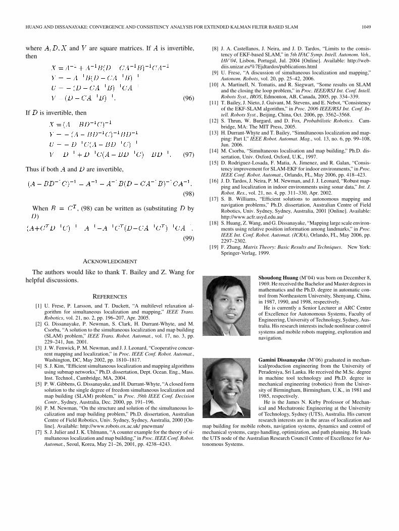
Shoudong Huang (M’04) was born on December 8,1969. He received the Bachelor and Master degrees inmathematics and the Ph.D. degree in automatic con-trol from Northeastern University, Shenyang, China,in 1987, 1990, and 1998, respectively.

He is currently a Senior Lecturer at ARC Centreof Excellence for Autonomous Systems, Faculty ofEngineering, University of Technology, Sydney, Aus-tralia. His research interests include nonlinear controlsystems and mobile robots mapping, exploration andnavigation.

Gamini Dissanayake (M’06) graduated in mechan-ical/production engineering from the University ofPeradeniya, Sri Lanka. He received the M.Sc. degreein machine tool technology and Ph.D. degree inmechanical engineering (robotics) from the Univer-sity of Birmingham, Birmingham, U.K., in 1981 and1985, respectively.

He is the James N. Kirby Professor of Mechan-ical and Mechatronic Engineering at the Universityof Technology, Sydney (UTS), Australia. His currentresearch interests are in the areas of localization and

map building for mobile robots, navigation systems, dynamics and control ofmechanical systems, cargo handling, optimization, and path planning. He leadsthe UTS node of the Australian Research Council Centre of Excellence for Au-tonomous Systems.