Scilab Textbook Companion forControl Systems Engineering
by Nagrath I.J. and Gopal M. 1
Created byAnuj Sharma
B.E. (pursuing)Electrical Engineering
Delhi Technological UniversityCollege Teacher
Ram Bhagat, DTU, DelhiCross-Checked by
sonanaya tatikola, IITB
June 28, 2012
1Funded by a grant from the National Mission on Education through ICT,http://spoken-tutorial.org/NMEICT-Intro. This Textbook Companion and Scilabcodes written in it can be downloaded from the ”Textbook Companion Project”section at the website http://scilab.in
Book Description
Title: Control Systems Engineering
Author: Nagrath I.J. and Gopal M.
Publisher: New Age Publisher, Delhi
Edition: 3
Year: 2007
ISBN: 81-224-1192-4
1
Scilab numbering policy used in this document and the relation to theabove book.
Exa Example (Solved example)
Eqn Equation (Particular equation of the above book)
AP Appendix to Example(Scilab Code that is an Appednix to a particularExample of the above book)
For example, Exa 3.51 means solved example 3.51 of this book. Sec 2.3 meansa scilab code whose theory is explained in Section 2.3 of the book.
2
Contents
List of Scilab Codes 4
2 Mathematical Models of Physical Systems 9
3 Feedback Characteristics of control sytems 11
5 Time Response analysis design specifications and perfor-mance indices 15
6 Concepts of stability and Algebraic Criteria 21
7 The Root Locus Technique 30
9 Stability in Frequency Domain 42
10 Introduction to Design 61
12 State Variable Analysis and Design 75
3
List of Scilab Codes
Exa 2.3 signal flow graph . . . . . . . . . . . . . . . . . . . . . 9Exa 2.4 transfer function . . . . . . . . . . . . . . . . . . . . . 9Exa 3.2 sensitivity of transfer function . . . . . . . . . . . . . . 11Exa 3.3.a sensitivity of transfer function . . . . . . . . . . . . . . 11Exa 3.3.b steady state error . . . . . . . . . . . . . . . . . . . . 12Exa 3.3.c calculation of slope . . . . . . . . . . . . . . . . . . . . 12Exa 3.3.d calculation of slope . . . . . . . . . . . . . . . . . . . . 13Exa 3.3.f calculation of input . . . . . . . . . . . . . . . . . . . 13Exa 3.3.g calculation of time . . . . . . . . . . . . . . . . . . . . 14Exa 5.2 steady state error . . . . . . . . . . . . . . . . . . . . 15Exa 5.2.2 steady state error . . . . . . . . . . . . . . . . . . . . 16Exa 5.3 transfer function . . . . . . . . . . . . . . . . . . . . . 16Exa 5.3.2 transfer function . . . . . . . . . . . . . . . . . . . . . 17Exa 5.4.1 steady state error . . . . . . . . . . . . . . . . . . . . 17Exa 5.4.2 steady state error . . . . . . . . . . . . . . . . . . . . 18Exa 5.4.3 steady state error . . . . . . . . . . . . . . . . . . . . 18Exa 5.8 steady state error . . . . . . . . . . . . . . . . . . . . 19Exa 5.9 state variable analysis . . . . . . . . . . . . . . . . . . 19Exa 6.1 hurwitz criterion . . . . . . . . . . . . . . . . . . . . . 21Exa 6.2 routh array . . . . . . . . . . . . . . . . . . . . . . . . 22Exa 6.3 routh array . . . . . . . . . . . . . . . . . . . . . . . . 22Exa 6.4 routh array . . . . . . . . . . . . . . . . . . . . . . . . 23Exa 6.5 routh array . . . . . . . . . . . . . . . . . . . . . . . . 23Exa 6.6 routh criterion . . . . . . . . . . . . . . . . . . . . . . 24Exa 6.7 routh array . . . . . . . . . . . . . . . . . . . . . . . . 25Exa 6.8 routh array . . . . . . . . . . . . . . . . . . . . . . . . 26Exa 6.9 routh array . . . . . . . . . . . . . . . . . . . . . . . . 26Exa 6.10 routh array . . . . . . . . . . . . . . . . . . . . . . . . 27
4
Exa 6.11.a routh array . . . . . . . . . . . . . . . . . . . . . . . . 27Exa 6.11.b routh array . . . . . . . . . . . . . . . . . . . . . . . . 28Exa 7.1 root locus . . . . . . . . . . . . . . . . . . . . . . . . . 30Exa 7.2 root locus . . . . . . . . . . . . . . . . . . . . . . . . . 30Exa 7.3 root locus . . . . . . . . . . . . . . . . . . . . . . . . . 32Exa 7.4 root locus . . . . . . . . . . . . . . . . . . . . . . . . . 33Exa 7.6 root locus . . . . . . . . . . . . . . . . . . . . . . . . . 35Exa 7.8 root locus . . . . . . . . . . . . . . . . . . . . . . . . . 37Exa 7.9 root locus . . . . . . . . . . . . . . . . . . . . . . . . . 39Exa 7.10 root locus . . . . . . . . . . . . . . . . . . . . . . . . . 39Exa 9.1 nyquist plot . . . . . . . . . . . . . . . . . . . . . . . . 42Exa 9.2 nyquist plot . . . . . . . . . . . . . . . . . . . . . . . . 42Exa 9.3 nyquist plot . . . . . . . . . . . . . . . . . . . . . . . . 44Exa 9.4 nyquist plot . . . . . . . . . . . . . . . . . . . . . . . . 45Exa 9.5 nyquist plot . . . . . . . . . . . . . . . . . . . . . . . . 47Exa 9.6 stability using nyquist plot . . . . . . . . . . . . . . . 49Exa 9.7.a stability using nyquist plot . . . . . . . . . . . . . . . 51Exa 9.7.b stability using nyquist plot . . . . . . . . . . . . . . . 52Exa 9.8.a nyquist criterion . . . . . . . . . . . . . . . . . . . . . 53Exa 9.8.b nyquist criterion . . . . . . . . . . . . . . . . . . . . . 53Exa 9.10 gm and pm using nyquist plot . . . . . . . . . . . . . . 53Exa 9.11 bode plot . . . . . . . . . . . . . . . . . . . . . . . . . 55Exa 9.13.a bode plot . . . . . . . . . . . . . . . . . . . . . . . . . 56Exa 9.13.b bode plot . . . . . . . . . . . . . . . . . . . . . . . . . 57Exa 9.14 m circles . . . . . . . . . . . . . . . . . . . . . . . . . 58Exa 9.15 m circles . . . . . . . . . . . . . . . . . . . . . . . . . 59Exa 10.6 lead compensation . . . . . . . . . . . . . . . . . . . . 61Exa 10.7 lead compensation . . . . . . . . . . . . . . . . . . . . 64Exa 10.8 lag compnsation . . . . . . . . . . . . . . . . . . . . . 67Exa 10.9 lag and lead compensation . . . . . . . . . . . . . . . 70Exa 12.3 state matrix . . . . . . . . . . . . . . . . . . . . . . . 75Exa 12.4 modal matrix . . . . . . . . . . . . . . . . . . . . . . . 75Exa 12.5 obtain time response . . . . . . . . . . . . . . . . . . . 76Exa 12.6 resolvant matrix . . . . . . . . . . . . . . . . . . . . . 77Exa 12.7 state transition matrix and state response . . . . . . . 77Exa 12.12 check for controllability . . . . . . . . . . . . . . . . . 78Exa 12.13 check for controllability . . . . . . . . . . . . . . . . . 79Exa 12.14 check for observability . . . . . . . . . . . . . . . . . . 79
5

Exa 12.17 design state observer . . . . . . . . . . . . . . . . . . . 80
6
List of Figures
7.1 root locus . . . . . . . . . . . . . . . . . . . . . . . . . . . . 317.2 root locus . . . . . . . . . . . . . . . . . . . . . . . . . . . . 327.3 root locus . . . . . . . . . . . . . . . . . . . . . . . . . . . . 337.4 root locus . . . . . . . . . . . . . . . . . . . . . . . . . . . . 347.5 root locus . . . . . . . . . . . . . . . . . . . . . . . . . . . . 357.6 root locus . . . . . . . . . . . . . . . . . . . . . . . . . . . . 367.7 root locus . . . . . . . . . . . . . . . . . . . . . . . . . . . . 387.8 root locus . . . . . . . . . . . . . . . . . . . . . . . . . . . . 40
9.1 nyquist plot . . . . . . . . . . . . . . . . . . . . . . . . . . . 439.2 nyquist plot . . . . . . . . . . . . . . . . . . . . . . . . . . . 449.3 nyquist plot . . . . . . . . . . . . . . . . . . . . . . . . . . . 459.4 nyquist plot . . . . . . . . . . . . . . . . . . . . . . . . . . . 469.5 nyquist plot . . . . . . . . . . . . . . . . . . . . . . . . . . . 479.6 nyquist plot . . . . . . . . . . . . . . . . . . . . . . . . . . . 489.7 stability using nyquist plot . . . . . . . . . . . . . . . . . . 509.8 stability using nyquist plot . . . . . . . . . . . . . . . . . . 519.9 stability using nyquist plot . . . . . . . . . . . . . . . . . . 529.10 gm and pm using nyquist plot . . . . . . . . . . . . . . . . . 549.11 bode plot . . . . . . . . . . . . . . . . . . . . . . . . . . . . 559.12 bode plot . . . . . . . . . . . . . . . . . . . . . . . . . . . . 569.13 bode plot . . . . . . . . . . . . . . . . . . . . . . . . . . . . 579.14 m circles . . . . . . . . . . . . . . . . . . . . . . . . . . . . . 589.15 m circles . . . . . . . . . . . . . . . . . . . . . . . . . . . . . 60
10.1 lead compensation . . . . . . . . . . . . . . . . . . . . . . . 6210.2 lead compensation . . . . . . . . . . . . . . . . . . . . . . . 6310.3 lead compensation . . . . . . . . . . . . . . . . . . . . . . . 6510.4 lead compensation . . . . . . . . . . . . . . . . . . . . . . . 66
7
10.5 lag compnsation . . . . . . . . . . . . . . . . . . . . . . . . . 6810.6 lag compnsation . . . . . . . . . . . . . . . . . . . . . . . . . 6910.7 lag and lead compensation . . . . . . . . . . . . . . . . . . . 7110.8 lag and lead compensation . . . . . . . . . . . . . . . . . . . 72
8
Chapter 2
Mathematical Models ofPhysical Systems
Scilab code Exa 2.3 signal flow graph
1 s=%s;
2 syms L C R1 R2
3 // fo rward path denoted by P ! and l oop by L1 , L2 andso on
4 // path f a c t o r by D1 and graph de t e rminant by D5 P1=1/(s*L*s*C);
6 L1=-R1/(s*L);
7 L2=-1/(s*R2*C);
8 L3=-1/(s^2*L*C);
9 D1=1;
10 D=1-(L1+L2+L3);
11 Y=(P1*D1)/D;
12 disp(Y,” T r a n s f e r f u n c t i o n=”)
Scilab code Exa 2.4 transfer function
9
1 syms xv Qf Qo Cf Co V Qw Kv
2 Qo=Qw+Qf;
3 // r a t e o f s a l t i n f l o w4 mi=Qf*Cf;
5 // r a t e o f s a l t o u t f l o w6 mo=Qo*Co;
7 // r a t e o f s a l t a c cumu la t i on8 ma=diff(V*Co ,t);
9 mi=ma+mo;
10 Qf*Cf=V*diff(Co,t)+Qo*Co;
11 Qf=Kv*xv;
12 K=Cf*Kv/Qo;
13 G=V/Qo;
14 G*diff(Co,t)+Co=K*xv;
15 // t a k i n g l a p l a c e16 G*s*Co+Co=K*xv;
17 // t r a n s f e r f u n c t i o n= Co/xv18 Co/xv=K/(G*s+1);
10
Chapter 3
Feedback Characteristics ofcontrol sytems
Scilab code Exa 3.2 sensitivity of transfer function
1 syms K;
2 s=%s;
3 G=syslin( ’ c ’ ,25(s+1)/(s+5));4 p=K;
5 q=s^2+s;
6 J=p/q;
7 F=G*J;
8 T=F/(1+F); // Closed l oop t r a n s f e r f u n c t i o n9 disp(T,”C( s ) /R( s ) ”)
10 // s e n s i t i v i t y w . r . t K = dT/dK∗K/T11 S=(diff(T,K))*(K/T)
12 disp(S,” S e n s i t i v i t y ”)
Scilab code Exa 3.3.a sensitivity of transfer function
1 syms K1 K t;
11
2 s=%s;
3 p=K1*K;
4 q=t*s+1+(K1*K);
5 T=p/q;
6 disp(T,”V( s ) /R( s ) ”)7 // s e n s i t i v i t y w . r . t K i s dT/dK∗K/T8 S=(diff(T,K))*(K/T)
9 // g i v e n K1=50 K=1.510 s=0
11 S=horner(S,s)
12 K1=50;
13 K=1.5;
14 S=1/(1+ K1*K)
15 disp(S,” s e n s i t i v i t y=”)
Scilab code Exa 3.3.b steady state error
1 syms A K K1 t
2 s=%s;
3 p=K1*K*A;
4 q=s*(1+(t*s)+(K1*K));
5 K=1.5;
6 K1=50;
7 V=p/q
8 v=limit(s*V,s,0)
9 // g i v e n s t eady s t a t e speed = 60km/ hr10 A=60*(1+( K1*K))/(K1*K)
11 // s t eady e r r o r e ( s s )=A−v12 v=60;
13 e=A-v;
14 disp(e,” e ( s s )=”)
Scilab code Exa 3.3.c calculation of slope
12
1 // under s t a l l e d c o n d i t i o n s2 syms Kg K1 D;
3 A=60.8;
4 A*K1=Kg*D;
5 // g i v e n Kg=1006 Kg=100;
7 K1=50;
8 D=(A*K1)/Kg;
9 disp(D,” u p s l o p e=”)
Scilab code Exa 3.3.d calculation of slope
1 // s t eady speed =10km/ hr2 syms K Kg D
3 (((A-10)*K1) -(-D*Kg))K=100;
4 A=(60.8*10) /60;
5 K=1.5;
6 Kg=100;
7 D=((100/K) -((A-10)*K))/Kg;
8 disp(D,”Down s l o p e=”)
Scilab code Exa 3.3.f calculation of input
1 // f o r open l oop system2 // g i v e n speed =60km/ hr3 syms R K1 K;
4 (R*K1*K)=60
5 K1=50;
6 K=1.5;
7 R=60/( K1*K)
8 disp(R,” Input open=”)9 // f o r c l o s e d l oop
10 R=60(1+( K1*K))/(K1*K)
13
11 disp(R,” Input c l o s e d=”)
Scilab code Exa 3.3.g calculation of time
1 // f o r open l oop2 syms t g s;
3 s=%s;
4 K1=50;
5 K=1.5;
6 g=20;
7 V=syslin( ’ c ’ ,((K1*K)*0.8)/(s*((g*s)+1)))8 // t a k i n g i n v e r s e l a p l a c e9 v=ilaplace(V,s,t)
10 v=60(11 -%e^(-t/20))
11 // g i v e n v=90%12 v=0.9;
13 t=-20*log(1-v);
14 disp(t,” t ime open=”)15 // f o r c l o s e d l oop16 syms K’ g’
17 s=%s;
18 V=syslin( ’ c ’ ,(60.8*K’)/(s*((g’*s)+1)))19 // t a k i n g i n v e r s e l a p l a c e20 v=ilaplace(V,s,t)
21 // g i v e n22 K ’=75/76;
23 g ’=.263;
24 v=60(1 -%e^(-t/.263))
25 // at v=90%26 v=0.9;
27 t= -.263* log(1-(v/60));
28 disp(t,” t ime c l o s e d=”)
14
Chapter 5
Time Response analysis designspecifications and performanceindices
Scilab code Exa 5.2 steady state error
1 s=%s
2 syms K J f
3 K=60; // g i v e n4 J=10; // g i v e n5 p=K/J
6 q=K/J+(f/J)*s+s^2
7 G=p/q;
8 disp(G,”Qo( s ) /Qi ( s )=”)9 zeta =0.3; // g i v e n
10 cof1=coeffs(q, ’ s ’ ,0)11 // on comparing the c o e f f i c i e n t s12 Wn=sqrt(cof1)
13 cof2=coeffs(q, ’ s ’ ,1)14 // 2∗ z e t a ∗Wn=c o f 215 f/J=2* zeta*Wn
16 r=s^2+f/J
17 s=s^2+f/J+K/J
15
18 H=r/s;
19 disp(H,”Qe( s ) /Qi ( s )=”)
Scilab code Exa 5.2.2 steady state error
1 // g i v e n Qi ( s ) =0.04/ s ˆ22 Qi =0.04/s^2;
3 e=limit(s*Qi*H,s,0)
4 disp(e,” Steady s t s t e e r o r=”)
Scilab code Exa 5.3 transfer function
1 s=%s;
2 syms Kp Ka Kt J f
3 // g i v e n4 J=0.4;
5 Kp=0.6;
6 Kt=2;
7 f=2;
8 p=Kp*Ka*Kt
9 q=s^2+f/J+(Kp*Ka*Kt)/J
10 G=p/q;
11 disp(G,”Qm( s ) /Qr ( s )=”)12 cof_1=coeffs(q, ’ s ’ ,0)13 // on comparing the c o e f f i c i e n t s14 // Wn=s q r t ( c o f 1 )15 Wn=10;
16 Ka=(Wn)^2*J/(Kp*f)
17 disp(Ka,” A m p l i f i e r Constant=”)
16
Scilab code Exa 5.3.2 transfer function
1 s=%s;
2 syms Kp Ka Kt Kd J f
3 // g i v e n4 J=0.4;
5 Kp=0.6;
6 Kt=2;
7 f=2;
8 Ka=5;
9 p=Kp*Ka*Kt
10 q=s^2+((f+Ka*Kd*Kt)/J)*s+(Kp*Ka*Kt)/J
11 G=p/q;
12 disp(G,”Qm( s ) /Qr ( s )=”)13 cof_1=coeffs(q, ’ s ’ ,0)14 // on comparing the c o e f f i c i e n t s15 Wn=sqrt(cof_1)
16 zeta=1 // g i v e n17 cof_2=coeffs(q, ’ s ’ ,1)18 // 2∗ z e t a ∗Wn=c o f 219 Kd=(2* zeta*sqrt(Kp*J*Ka*Kt)-f)/(Ka*Kt)
20 disp(Kd,” Tachogene r to r c o n s t a n t=”)
Scilab code Exa 5.4.1 steady state error
1 syms Wn zeta Kv Ess
2 s=%s;
3 p=poly ([8 2 1], ’ s ’ , ’ c o e f f ’ ); // c h a r a c t e r i s t i ce q u a t i o n
4 z=coeff(p);
5 Wn=sqrt(z(1,1))
6 zeta=z(1,2) /(2*Wn)
7 Kv=z(1,1)/z(1,2)
8 Ess =1/Kv // Steady s t a t e e r r o r f o r u n i t ramp i /p9 disp(Ess ,” Steady s t a t e Er ro r=”)
17
Scilab code Exa 5.4.2 steady state error
1 // with d e r i v a t i v e f e e d b a c k2 // c h a r a c t e r i s t i c e q u a t i o n i s3 syms a
4 s=%s;
5 p=s^2+(2+(8*a))*s+8=0
6 zeta =0.7 // g i v e n7 Wn =2.828;
8 cof_1=coeffs(p, ’ s ’ ,1)9 // on comparing 2∗ z e t a ∗Wn=c o f 1
10 a=((2* zeta*Wn) -2)/8
11 disp(a,” D e r i v a t i v e f e e d b a c k=”)12 cof_2=coeffs(p, ’ s ’ ,0)13 cof_1 =2+8*0.245;
14 Kv=cof_2/cof_1;
15 Ess =1/Kv
16 disp(Ess ,” Steady s t a t e e r r o r=”)
Scilab code Exa 5.4.3 steady state error
1 // l e t the char e q u a t i o n be2 syms Ka
3 s=%s;
4 p=s^2+(2+(a*Ka))*s+Ka=0
5 cof_1=coeffs(p, ’ s ’ ,0)6 // Wnˆ2= c o f 17 Wn=sqrt(cof_1)
8 cof_2=coeffs(p, ’ s ’ ,1)9 // 2∗ z e t a ∗Wn=c o f 2
10 Kv=cof_1/cof_2;
18
11 Ess =1/Kv;
12 // g i v e n Ess =0.2513 Ess =0.25;
14 Ka=2/(Ess -a)
15 disp(Ka.”Ka=”)
Scilab code Exa 5.8 steady state error
1 s=%s;
2 syms K V
3 p=s^2+(100*K)*s+100=0
4 cof_1=coeffs(p, ’ s ’ ,0)5 Wn=sqrt(cof_1)
6 zeta=1 // g i v e n7 cof_2=coeffs(p, ’ s ’ ,1)8 // 2∗ z e t a ∗Wn=c o f 29 K=(2*Wn*zeta)/100
10 // For ramp input11 R=V/s^2
12 E=R/p
13 // s t eady s t a t e e r r o r14 e=limit(s*E(s),s,0)
15 disp(e,” e ( s s )=”)
Scilab code Exa 5.9 state variable analysis
1 s=%s;
2 syms t m
3 A=[0 1;-100 -20];
4 B=[0;100];
5 C=[1 0];
6 x=[0;0];
7 [r c]=size(A)
19
8 p=s*eye(r,c)-A
9 q=inv(p);
10 disp(q,” ph i ( s )=”) // Reso lvant matr ix11 for i=1:r;
12 for j=1:c;
13 q(i,j)=ilaplace(q(i,j),s,t)
14 end
15 end
16 disp(q,” ph i ( t )=”) // S t a t e t r a n s i t i o n matr ix17 t=t-m;
18 q=eval(q)
19 // I n t e g r a t e q w. r . t m20 r=integrate(q*B,m)
21 m=0 // Upper l i m i t i s t22 g=eval(r) // Put ing upper l i m i t i n q23 m=t // Lower l i m i t i s 024 h=eval(r) // Put t ing l owe r l i m i t i n q25 y=(h-g);
26 disp(y,”y=”)27 printf(”x ( t )=phi ( t ) ∗x ( 0 )+i n t e g r a t e ( ph i ( t−m∗B) w. r . t
m from 0 to t ) ”)28 y1=(q*x)+y;
29 disp(y1,”x ( t )=”)30 // t r a n s f e r f u n c t i o n31 t=C*q*B;
32 disp(t,”T( s )=”)
20
Chapter 6
Concepts of stability andAlgebraic Criteria
Scilab code Exa 6.1 hurwitz criterion
1 s=%s;
2 p=s^4+8*s^3+18*s^2+16*s+5
3 r=coeff(p)
4 D1=r(4)
5 d2=[r(4) r(5);r(2) r(3)]
6 D2=det(d2);
7 d3=[r(4) r(5) 0;r(2) r(3) r(4);0 r(1) r(2)]
8 D3=det(d3);
9 d4=[r(4) r(5) 0 0;r(2) r(3) r(4) r(5);0 r(1) r(2) r
(3);0 0 0 r(1)]
10 D4=det(d4);
11 disp(D1,”D1=”)12 disp(D2,”D2=”)13 disp(D3,”D3=”)14 disp(D4,”D4=”)15 printf(” S i n c e a l l the d e t e r m i n a n t s a r e p o s i t i v e the
system i s s t a b l e ”)
21
Scilab code Exa 6.2 routh array
1 s=%s;
2 p=s^4+8*s^3+18*s^2+16*s+5
3 r=routh_t(p)
4 m=coeff(p)
5 l=length(m)
6 c=0;
7 for i=1:l
8 if (r(i,1) <0)
9 c=c+1;
10 end
11 end
12 if(c>=1)
13 printf(” System i s u n s t a b l e ”)14 else (”Sysem i s s t a b l e ”)15 end
Scilab code Exa 6.3 routh array
1 s=%s;
2 p=3*s^4+10*s^3+5*s^2+5*s+2
3 r=routh_t(p)
4 m=coeff(p)
5 l=length(m)
6 c=0;
7 for i=1:l
8 if (r(i,1) <0)
9 c=c+1;
10 end
11 end
12 if(c>=1)
22
13 printf(” System i s u n s t a b l e ”)14 else (”Sysem i s s t a b l e ”)15 end
Scilab code Exa 6.4 routh array
1 s=%s;
2 syms Kv Kd Kp Kt
3 p=s^3+(1+( Kv*Kd))*s^2+(Kv*Kp)*s+(Kp*Kt)
4 cof_a_0=coeffs(p, ’ s ’ ,0);5 cof_a_1=coeffs(p, ’ s ’ ,1);6 cof_a_2=coeffs(p, ’ s ’ ,2);7 cof_a_3=coeffs(p, ’ s ’ ,3);8 r=[ cof_a_0 cof_a_1 cof_a_2 cof_a_3]
9 n=length(r);
10 routh=[r([4 ,2]);r([3 ,1])]
11 routh=[routh;-det(routh)/routh (2,1) ,0]
12 t=routh (2:3 ,1:2);
13 routh=[routh;-det(t)/routh (3,1) ,0]
14 disp(routh ,” routh=”);15 // f o r s t a b i l i t y r ( : , 1 ) >016 // f o r the g i v e n t a b l e17 b=routh (3,1)
18 disp(” f o r s t a b i l i t y ”b,”>0”)
Scilab code Exa 6.5 routh array
1 s=%s;
2 syms K
3 p=(1+K)*s^2+((3*K) -0.9)*s+(2K-1)
4 cof_a_0=coeffs(p, ’ s ’ ,0);5 cof_a_1=coeffs(p, ’ s ’ ,1);6 cof_a_2=coeffs(p, ’ s ’ ,2);
23
7 r=[ cof_a_0 cof_a_1 cof_a_2]
8 n=length(r);
9 routh=[r([3 ,1]);r(2) ,0];
10 routh=[routh;-det(routh)/routh (2,1) ,0];
11 disp(routh ,” routh=”)12 // f o r no r o o t i n r i g h t h a l f13 // routh ( 1 , 1 ) , routh ( 2 , 1 ) , routh ( 3 , 1 )>014 routh (1,1)=0
15 routh (2,1)=0
16 routh (3,1)=0
17 // combin ing the r e s u l t18 K=0.9/3;
19 disp(K,” For no r o o t s i n r i g h t h a l f=”)20 // f o r 1 p o l e i n r i g h t h a l f i . e . one s i g n change21 // routh ( 1 , 1 )>0 n routh ( 3 , 1 )<022 disp(” For one p o l e i n r i g h t h a l f , −1<K<0.05 ”)23 // f o r 2 p o l e s i n r i g h t h a l f24 // routh ( 2 , 1 )<0 n routh ( 3 , 1 )>025 disp(” For 2 p o l e s i n r i g h t h a l f , 0.05 <K<0.3 ”)
Scilab code Exa 6.6 routh criterion
1 s=%s;
2 syms K
3 p=s^2-(K+2)*s+((2*K)+5)
4 cof_a_0=coeffs(p, ’ s ’ ,0);5 cof_a_1=coeffs(p, ’ s ’ ,1);6 cof_a_2=coeffs(p, ’ s ’ ,2);7 r=[ cof_a_0 cof_a_1 cof_a_2]
8 n=length(r);
9 routh=[r([3 ,1]);r(2) ,0];
10 routh=[routh;-det(routh)/routh (2,1) ,0];
11 disp(routh ,” routh=”)12 // f o r system to be s t a b l e13 routh (2,1) >0
24
14 K<-2;
15 routh (3,1) >0
16 K>-2.5;
17 disp(” For s t a b l e system , −2>K>−2.5”)18 // f o r l i m i t e d s t a b i l i t y19 routh (2,1)=0
20 K=-2
21 routh (3,1)=0
22 K=-2.5
23 disp(” For l i m t e d s t a b l e system K=−2 and K=−2.5”)24 // f o r u n s t a b l e system25 disp(” For u n s t a b l e system K<−2 or K>−2.5”)26 roots(p) // g i v e s the r o o t s o f the po lynomia l m27 // f o r c r i t i c a l l y damped c a s e28 g=(K+2) ^2 -4*((2*K)+5)
29 roots(g)
30 // f o r s t a b l i t y K=6.47 i s u n s t a b l e31 // f o r c r i t i c a l damping K=−2.4732 disp(” For underdamded case , −2>K>−2.47”)33 disp(” f o r overdamped case , −2.47>K>−2.5”)
Scilab code Exa 6.7 routh array
1 s=%s;
2 syms eps
3 p=s^5+s^4+2*s^3+2*s^2+3*s+5
4 r=coeff(p);
5 n=length(r);
6 routh=[r([6,4,2]);r([5,3 ,1])]
7 syms eps;
8 routh=[routh;eps ,-det(routh (1:2 ,2:3))/routh (2,2) ,0];
9 routh=[routh;-det(routh (2:3 ,1:2))/routh (3,1) ,-det(
routh (2:3 ,2:3))/routh (4,2) ,0];
10 routh=[routh;-det(routh (4:5 ,1:2))/routh (5,1) ,0,0];
11 disp(routh ,” routh=”)
25
12 // to check s t a b i l i t y13 routh (4,1)=8-limit (5/eps ,eps ,0);
14 disp(routh (4,1),” routh ( 4 , 1 )=”)15 routh (5,1)=limit(routh (5,1),eps ,0);
16 disp(routh (5,1),” routh ( 5 , 1 )=”)17 printf(” There a r e two s i g n changes o f f i r s t column
hence the system i s u n s t a b l e ”)
Scilab code Exa 6.8 routh array
1 s=%s;
2 p=s^6+2*s^5+8*s^4+12*s^3+20*s^2+16*s+16
3 r=routh_t(p)
4 roots(p)
5 disp(0,” the number o f r e a l pa r t o f r o o t s l y i n g i nthe r i g h t h a l f ”)
6 printf(” System i s s t a b l e ”)
Scilab code Exa 6.9 routh array
1 s=%s;
2 syms K a
3 p=s^4+10*s^3+32*s^2+(K+32)*s+(K*a)
4 cof_a_0=coeffs(p, ’ s ’ ,0);5 cof_a_1=coeffs(p, ’ s ’ ,1);6 cof_a_2=coeffs(p, ’ s ’ ,2);7 cof_a_3=coeffs(p, ’ s ’ ,3);8 cof_a_4=coeffs(p, ’ s ’ ,4);9 r=[ cof_a_0 cof_a_1 cof_a_3 cof_a_4]
10 n=length(r);
11 routh=[r([5,3,1]);r([4 ,2]) ,0]
12 routh=[routh;-det(routh (1:2 ,1:2))/routh (2,1) ,-det(
routh (1:2 ,2:3))/routh (2,2) ,0];
26
13 routh=[routh;-det(routh (2:3 ,1:2))/routh (3,1) ,-det(
routh (2:3 ,2:3))/routh (3,2) ,0];
14 routh=[routh;-det(routh (3:4 ,1:2))/routh (4,1) ,0,0];
15 disp(routh ,” routh=”)16 // f o r the g i v e n system to be s t a b l e17 routh (3,1) >0
18 K<288;
19 routh (4,1) >0
20 (288-K)*(K+32) -100(K*a)>0
21 // l e t K=20022 K=200;
23 a=((288 -K)*(K+32))/(100*K)
24 // v e l o c i t y e r r o r25 Kv=(K*a)/(4*2*4);
26 // % v e l o c i t y e r r o r27 Kvs =100/ Kv
28 disp(a,” c o n t r o l parameter=”)29 disp(K,” Gain=”)
Scilab code Exa 6.10 routh array
1 s=%s;
2 p=s^3+7*s^2+25*s+39
3 // to check i f the r o o t s l i e l e f t o f s=−14 // s u b s t i t u t e s=s−15 p=(s-1) ^3+7*(s-1) ^2+25*(s-1)+20
6 r=routh_t(p)
7 printf(” A l l the s i g n s o f e l e m e n t s f i r s t column a r ep o s i t i v e hence the r o o t s l i e l e f t o f s=−1”)
Scilab code Exa 6.11.a routh array
1 s=%s;
27
2 syms K
3 // the system c h a r a c t e r i s t i c eq can be w r i t t e n as4 p=s^3+8.5*s^2+20*s+12.5(1+K)
5 cof_a_0=coeffs(p, ’ s ’ ,0);6 cof_a_1=coeffs(p, ’ s ’ ,1);7 cof_a_2=coeffs(p, ’ s ’ ,2);8 cof_a_3=coeffs(p, ’ s ’ ,3);9 r=[ cof_a_0 cof_a_1 cof_a_2 cof_a_3]
10 n=length(r);
11 routh=[r([4 ,2]);r([3 ,1])]
12 routh=[routh;-det(routh)/routh (2,1) ,0]
13 t=routh (2:3 ,1:2);
14 routh=[routh;-det(t)/routh (3,1) ,0]
15 disp(routh ,” routh=”);16 // f o r l i m i t i n g v a l u e o f K17 routh (3,1)=0
18 K=12.6;
19 disp(K,” L i m i t i n g v a l u e o f K”)
Scilab code Exa 6.11.b routh array
1 syms zeta Wn ts z
2 // s e t t l i n g t ime t s =4/ z e t a ∗Wn3 // g i v e n t s =4 s e c4 ts=4;
5 zeta*Wn=ts/4
6 printf(”now the r e a l pa r t o f dominant r o o t shou ld be−1 or more”)
7 // s u b s t i t u t i n g s=s−18 p=(s-1) ^3+8.5*(s-1) ^2+20*(s-1) +12.5*(1+K)
9 cof_a_0=coeffs(p, ’ s ’ ,0);10 cof_a_1=coeffs(p, ’ s ’ ,1);11 cof_a_2=coeffs(p, ’ s ’ ,2);12 cof_a_3=coeffs(p, ’ s ’ ,3);13 r=[ cof_a_0 cof_a_1 cof_a_2 cof_a_3]
28
14 n=length(r);
15 routh=[r([4 ,2]);r([3 ,1])]
16 routh=[routh;-det(routh)/routh (2,1) ,0]
17 t=routh (2:3 ,1:2);
18 routh=[routh;-det(t)/routh (3,1) ,0]
19 disp(routh ,” routh=”);20 // f o r l i m i t i n g v a l u e o f K21 routh (3,1)=0
22 K=2.64
23 disp(K,” L i m i t i n g v a l u e o f K f o r s e t t l i n g t ime o f 4 s=”)
24 // r o o t s o f char eq at K=2.6425 g=s^3+8.5*s^2+20*s+12.5*(1+2.64)
26 roots(g)
29
Chapter 7
The Root Locus Technique
Scilab code Exa 7.1 root locus
1 s=%s;
2 syms k
3 H=syslin( ’ c ’ ,(k*(s+1)*(s+2))/(s*(s+3)*(s+4)));4 evans(H,5)
5 printf(” There a r e t h r e e b ranche s o f r o o t l o c u ss t a r t i n g with K=0 and p o l e s s =0 ,−3 ,−4. ”)
6 printf(”As k i n c r e a s e s two branche s t e r m i n a t e atz e r o s s=−1,−2 and one at i n f i n i t y ”)
Scilab code Exa 7.2 root locus
1 s=%s;
2 syms k
3 H=syslin( ’ c ’ ,1+(k/(s*(s+1)*(s+2))));4 evans(H,5)
30
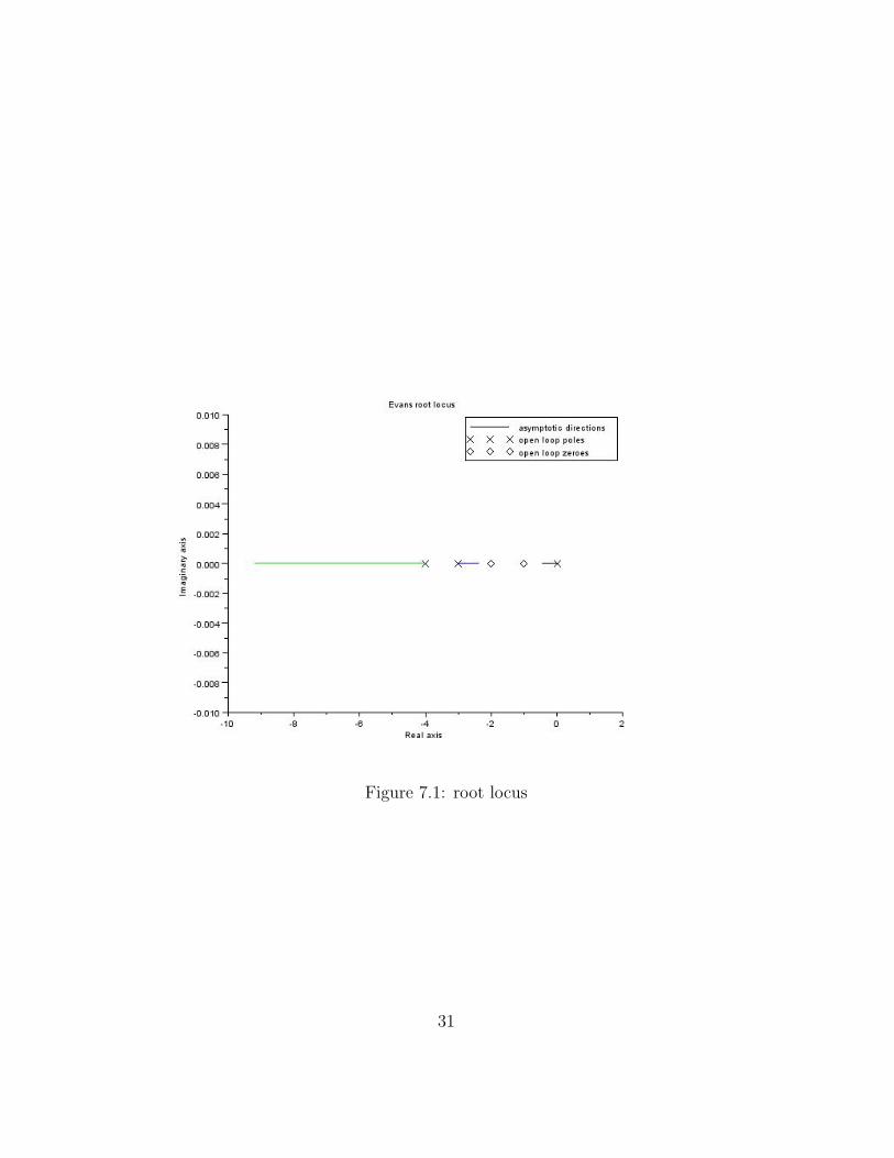
Figure 7.1: root locus
31
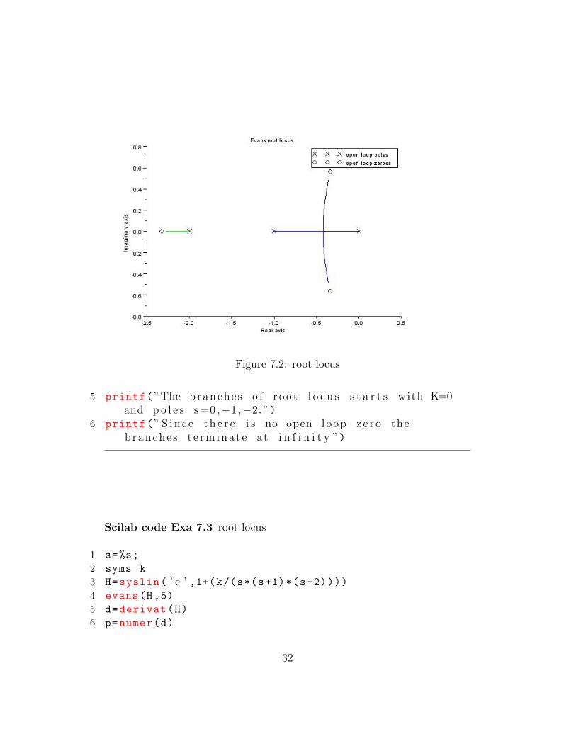
Figure 7.2: root locus
5 printf(”The branche s o f r o o t l o c u s s t a r t s with K=0and p o l e s s =0 ,−1 ,−2. ”)
6 printf(” S i n c e t h e r e i s no open l oop z e r o thebranche s t e r m i n a t e at i n f i n i t y ”)
Scilab code Exa 7.3 root locus
1 s=%s;
2 syms k
3 H=syslin( ’ c ’ ,1+(k/(s*(s+1)*(s+2))))4 evans(H,5)
5 d=derivat(H)
6 p=numer(d)
32
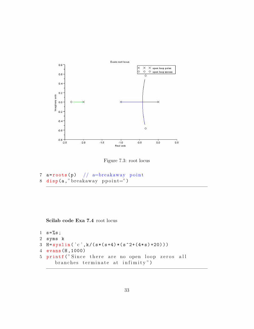
Figure 7.3: root locus
7 a=roots(p) // a=breakaway p o i n t8 disp(a,” breakaway ppo in t=”)
Scilab code Exa 7.4 root locus
1 s=%s;
2 syms k
3 H=syslin( ’ c ’ ,k/(s*(s+4)*(s^2+(4*s)+20)))4 evans(H ,1000)
5 printf(” S i n c e t h e r e a r e no open l oop z e r o s a l lb ranche s t e r m i n a t e at i n f i m i t y ”)
33
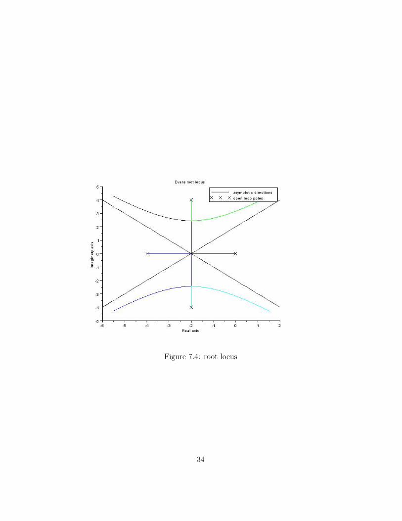
Figure 7.4: root locus
34
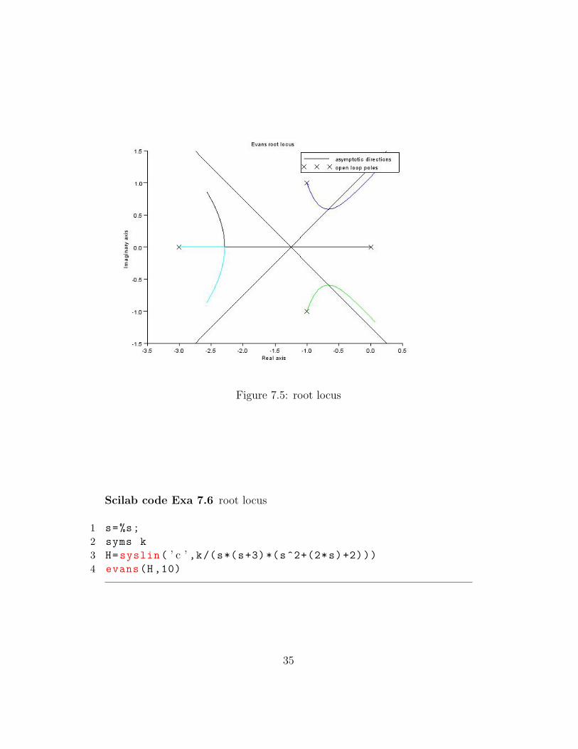
Figure 7.5: root locus
Scilab code Exa 7.6 root locus
1 s=%s;
2 syms k
3 H=syslin( ’ c ’ ,k/(s*(s+3)*(s^2+(2*s)+2)))4 evans(H,10)
35
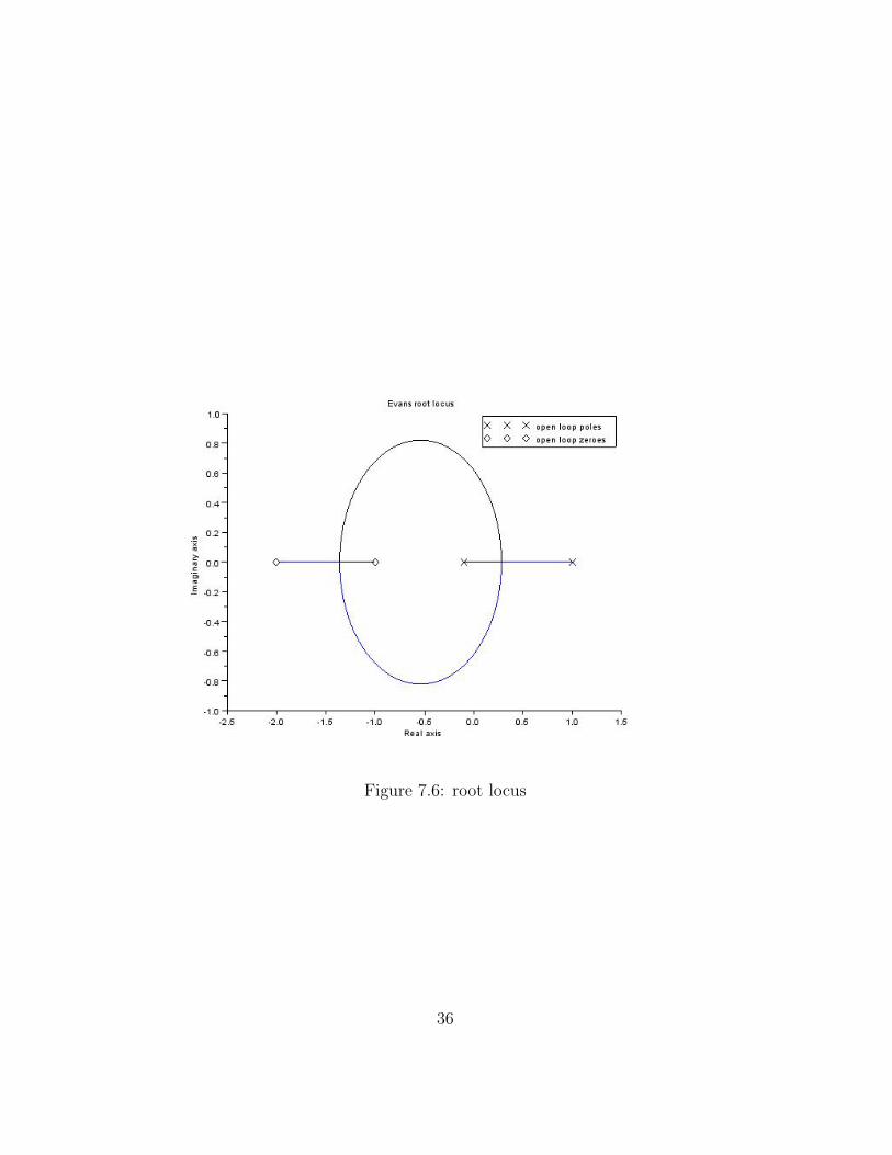
Figure 7.6: root locus
36
Scilab code Exa 7.8 root locus
1 syms K
2 s=%s;
3 G=syslin( ’ c ’ ,(K*(s+1)*(s+2))/((s+0.1)*(s-1)))4 evans(G)
5 n=2;
6 disp(n,”no o f p o l e s=”)7 m=2;
8 disp(m,”no o f z e r o e s=”)9 K=kpure(G)
10 disp(K,” v a l u e o f K where RL c r o s s e s jw a x i s=”)11 d=derivat(G)
12 p=numer(d)
13 a=roots(p); // a=breakaway p o i n t s14 disp(a,” breakaway p o i n t s=”)15 for i=1:2
16 K=-(a(i,1) +0.1) *(a(i,1) -1)/((a(i,1)+1)*(a(i,1)
+2))
17 disp(a(i,1),” s=”)18 disp(K,”K=”)19 end
20 printf(” z e t a =1 i s a c h i e v e d when the two r o o t s a r ee q u a l and n e g a t i v e ( r e a l ) . This happens at thebreakaway p o i n t i n the l e f t h a l f s−p lane /n”)
21 zeta =1;
22 wn=0.6;
23 sgrid(zeta ,wn)
24 K=-1/real(horner(G,[1 %i]* locate (1)));
25 disp(K,”The c o r r e s p o n d i n g v a l u e o f ga in i s=”)
37
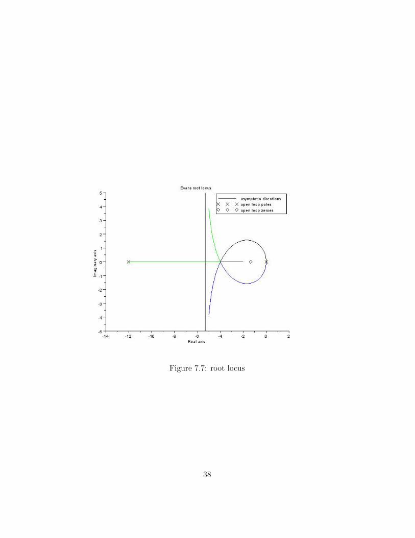
Figure 7.7: root locus
38
Scilab code Exa 7.9 root locus
1 syms K
2 s=%s;
3 G=syslin( ’ c ’ ,(K*(s+4/3))/(s^2*(s+12)))4 evans(G,60)
5 d=derivat(G)
6 p=numer(d)
7 a=roots(p) // a=breakaway p o i n t s8 disp(a,” Breakaway p o i n t s=”)9 printf(” Equal r o o t s a r e at s=−4”)
10 printf(”/n Value o f K at s=−4=”)11 K=4*4*8/(4 -(4/3))
12 disp(K)
Scilab code Exa 7.10 root locus
1 syms Kh
2 s=%s;
3 G=syslin( ’ c ’ ,10*Kh*(s+0.04) *(s+1)/((s+0.5) *(s^2 -(0.4*s)+0.2) *(s+8)));
4 evans(G,3)
5 Kh=kpure(G)
6 K=10*Kh
7 zeta =1/(2) ^(1/2);
8 wn =.575;
9 sgrid(zeta ,wn)
10 K=-1/real ((2* horner(G,[1 %i]* locate (1))));
11 printf(”The z e t a =1/(2) ˆ1/2 l i n e i n t e r s e c t s the r o o tl o c u s at two p o i n t s with K1=1.155 and K2=0.79 ”)
39
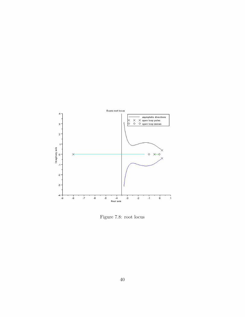
Figure 7.8: root locus
40
12 Kh1 =0.156;
13 Kh2 =0.079;
14 // from the b l o c k diagram15 Td(s)=1/s;
16 E(s)=C(s)=G/(1+(G*Kh*(s+1))/(s+8))*Td(s);
17 // s u b s t i t u t i n g v a l u e o f G18 F=s*E(s)=10*Kh /(1+(10* Kh));
19 // s t e a y s t a t e e r r o r20 ess=limit(F,s,0)
21 // f o r Kh1=0.15622 ess =0.609;
23 // f o r Kh2=0.07924 ess =0.44;
41
Chapter 9
Stability in Frequency Domain
Scilab code Exa 9.1 nyquist plot
1 s=%s;
2 syms K T1 T2
3 H=syslin( ’ c ’ ,K/((T1*s+1)*(T2*s+1)));4 nyquist(H)
5 show_margins(H, ’ n y q u i s t ’ )6 printf(” S i n c e P=0(no o f p o l e s i n RHP) and the
n y q u i s t con tour does not e n c i r c l e the p o i n t −1+j 0”)
7 printf(” System i s s t a b l e ”)
Scilab code Exa 9.2 nyquist plot
1 s=%s;
2 H=syslin( ’ c ’ ,(s+2) /((s+1)*(s-1)))3 nyquist(H)
42
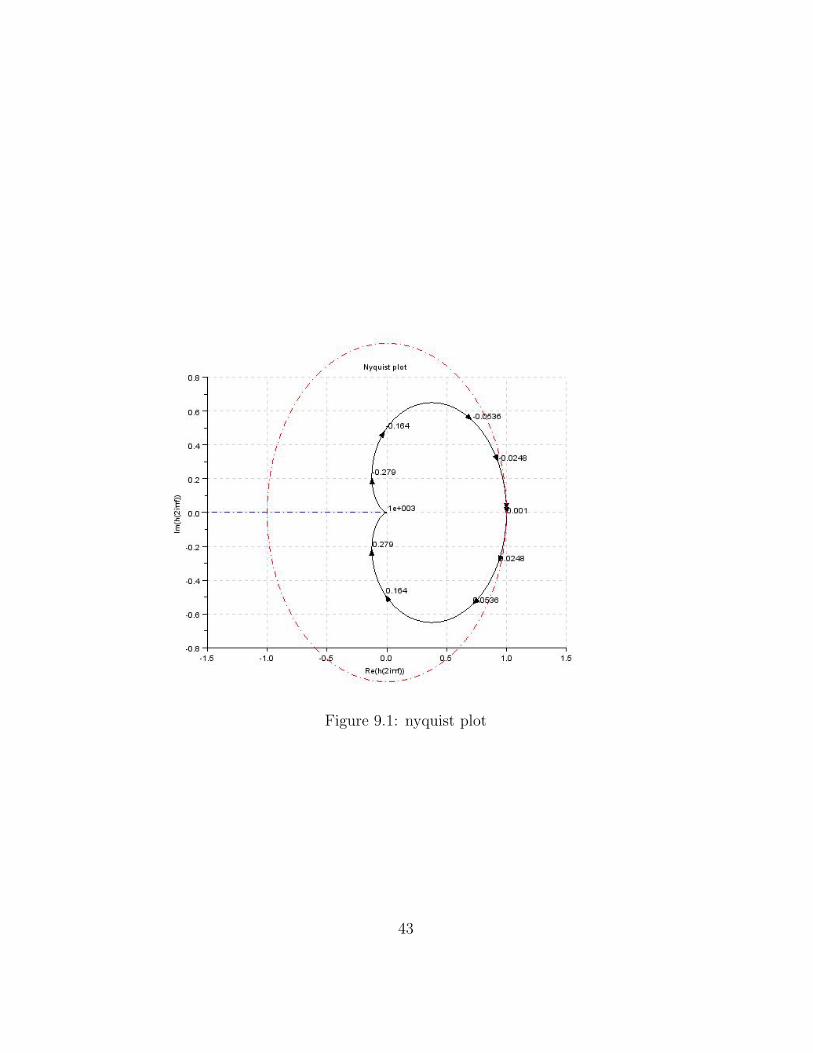
Figure 9.1: nyquist plot
43
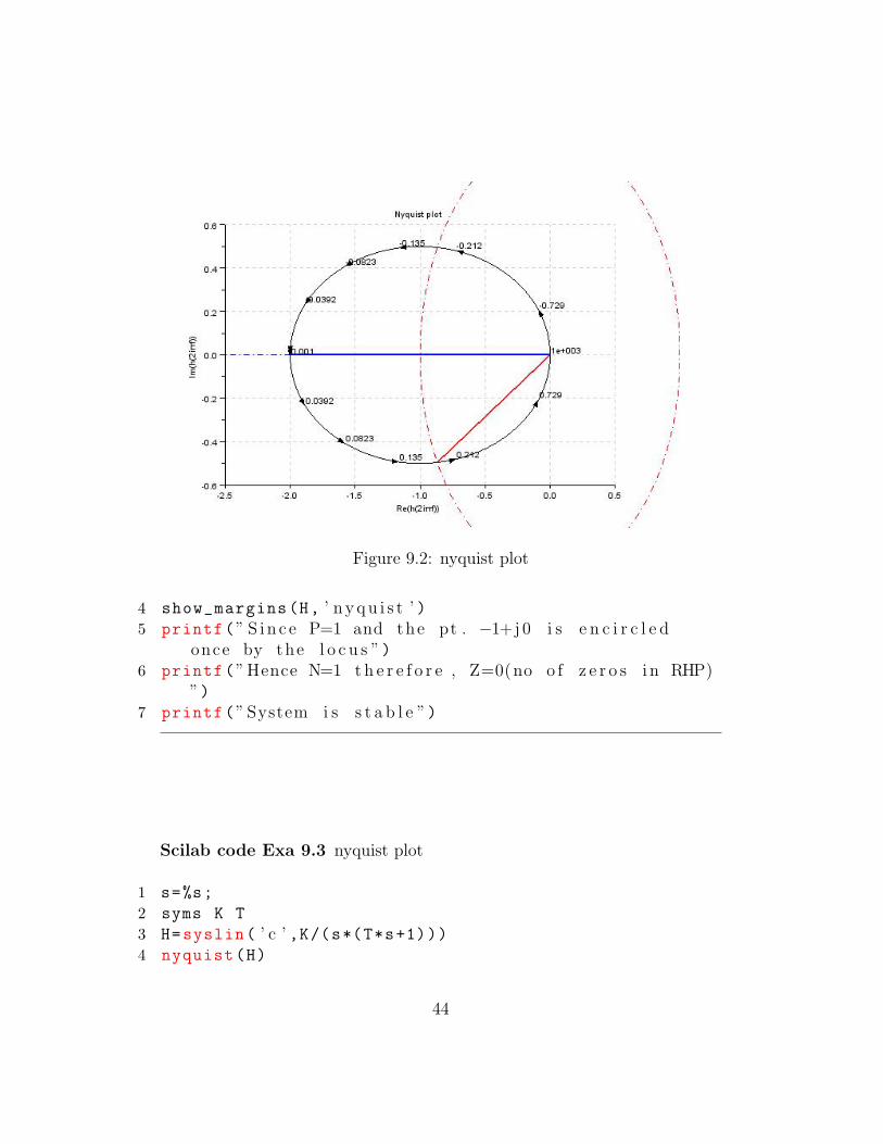
Figure 9.2: nyquist plot
4 show_margins(H, ’ n y q u i s t ’ )5 printf(” S i n c e P=1 and the pt . −1+j 0 i s e n c i r c l e d
once by the l o c u s ”)6 printf(” Hence N=1 t h e r e f o r e , Z=0(no o f z e r o s i n RHP)
”)7 printf(” System i s s t a b l e ”)
Scilab code Exa 9.3 nyquist plot
1 s=%s;
2 syms K T
3 H=syslin( ’ c ’ ,K/(s*(T*s+1)))4 nyquist(H)
44
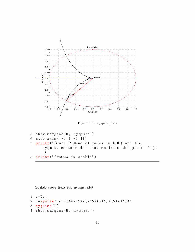
Figure 9.3: nyquist plot
5 show_margins(H, ’ n y q u i s t ’ )6 mtlb_axis ([-1 1 -1 1])
7 printf(” S i n c e P=0(no o f p o l e s i n RHP) and then y q u i s t con tour does not e n c i r c l e the p o i n t −1+j 0”)
8 printf(” System i s s t a b l e ”)
Scilab code Exa 9.4 nyquist plot
1 s=%s;
2 H=syslin( ’ c ’ ,(4*s+1)/(s^2*(s+1) *(2*s+1)))3 nyquist(H)
4 show_margins(H, ’ n y q u i s t ’ )
45
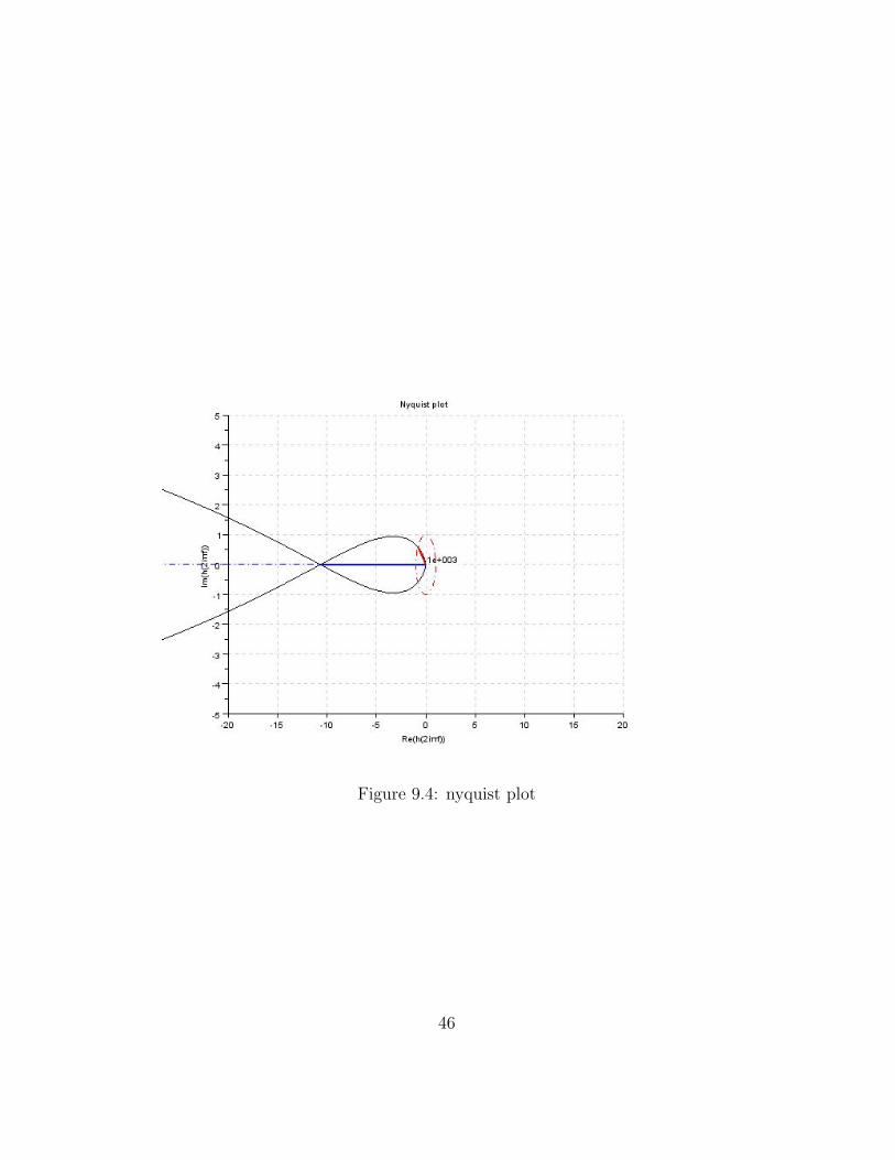
Figure 9.4: nyquist plot
46
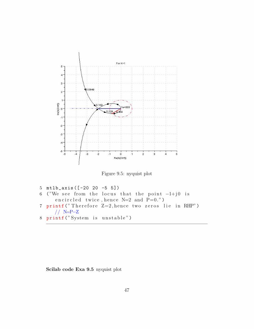
Figure 9.5: nyquist plot
5 mtlb_axis ([-20 20 -5 5])
6 (”We s e e from the l o c u s tha t the p o i n t −1+j 0 i se n c i r c l e d twice , hence N=2 and P=0. ”)
7 printf(” T h e r e f o r e Z=2 , hence two z e r o s l i e i n RHP”)// N=P−Z
8 printf(” System i s u n s t a b l e ”)
Scilab code Exa 9.5 nyquist plot
47
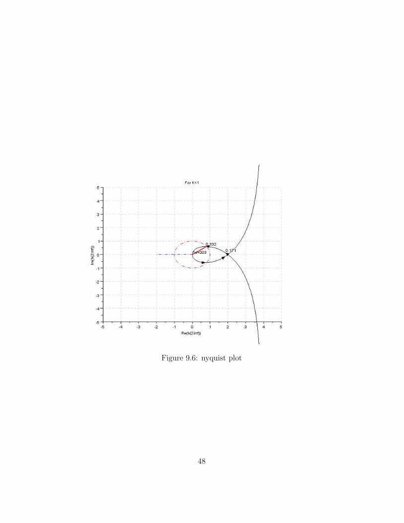
Figure 9.6: nyquist plot
48
1 s=%s;
2 syms K a
3 H=syslin( ’ c ’ ,(K*(s+a))/(s*(s-1)))4 // f o r K>15 nyquist(H)
6 show_margins(H, ’ n y q u i s t ’ )7 mtlb_axis ([-5 5 -5 5])
8 xtitle(” For K>1”)9 printf(”P=1( p o l e i n RHP) )
10 p r i n t f ( ” Nyquist plot encircles the the point -1+j0
once anti -clockwise i.e.,N=1” )11 p r i n t f ( ”Hence Z=0” ) // N=P−Z12 p r i n t f ( ”System is stable ” )13 // f o r K<114 H=s y s l i n ( ’ c ’ , ( −2∗ ( s +1) ) /( s ∗ ( s−1) ) )15 show marg ins (H, ’ nyqu i s t ’ )16 m t l b a x i s ([−5 5 −5 5 ] )17 x t i t l e ( ”For K<1” )18 p r i n t f ( ”The point -1+j0 lie beyond -K(the crossing
point of the plot).So N=-1,P=1” )19 p r i n t f ( ”Hence Z=2,zeros in RHP=2” )20 p r i n t f ( ”System is unstable ” )
Scilab code Exa 9.6 stability using nyquist plot
1 s=%s;
2 syms k
3 H=syslin( ’ c ’ ,(k*(s-2))/(s+1) ^2)4 // f o r K/2>−1 or K>−25 nyquist(H)
6 show_margins(H, ’ n y q u i s t ’ )7 printf(”P=0( p o l e s i n RHP) ”)8 printf(”N=−1, hence Z=1”)
49
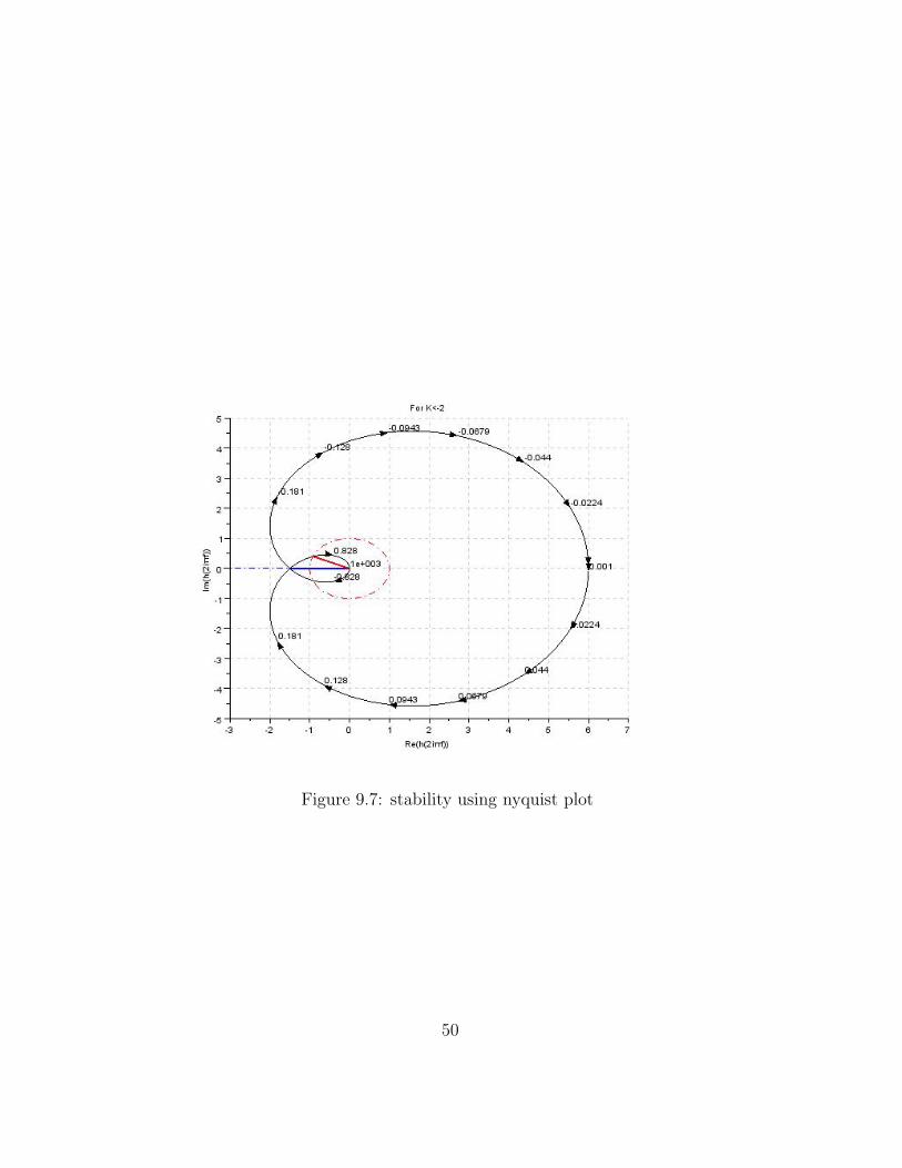
Figure 9.7: stability using nyquist plot
50
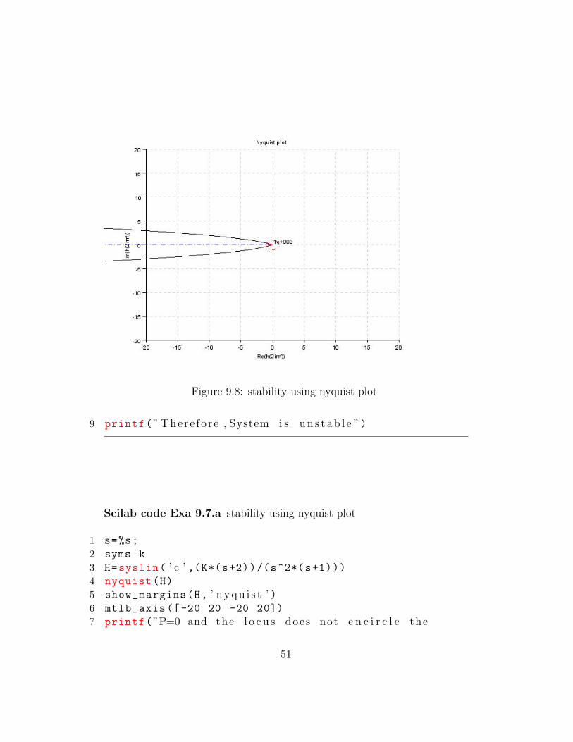
Figure 9.8: stability using nyquist plot
9 printf(” Ther e f o r e , System i s u n s t a b l e ”)
Scilab code Exa 9.7.a stability using nyquist plot
1 s=%s;
2 syms k
3 H=syslin( ’ c ’ ,(K*(s+2))/(s^2*(s+1)))4 nyquist(H)
5 show_margins(H, ’ n y q u i s t ’ )6 mtlb_axis ([-20 20 -20 20])
7 printf(”P=0 and the l o c u s does not e n c i r c l e the
51
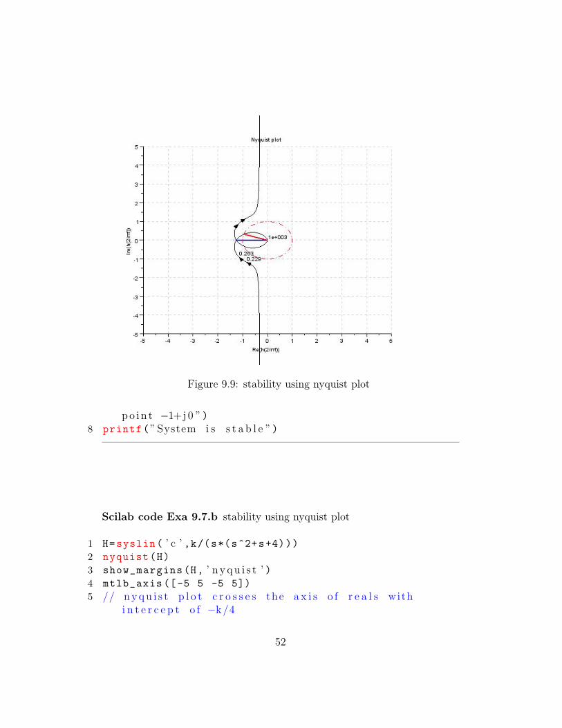
Figure 9.9: stability using nyquist plot
p o i n t −1+j 0 ”)8 printf(” System i s s t a b l e ”)
Scilab code Exa 9.7.b stability using nyquist plot
1 H=syslin( ’ c ’ ,k/(s*(s^2+s+4)))2 nyquist(H)
3 show_margins(H, ’ n y q u i s t ’ )4 mtlb_axis ([-5 5 -5 5])
5 // n y q u i s t p l o t c r o s s e s the a x i s o f r e a l s withi n t e r c e p t o f −k/4
52
6 // f o r k/4>1 or k>47 printf(”N=−2 as i t e n c i r c l e s the p o i n t t w i c e i n
c l o c k w i s e d i r e c t i o n ”)8 printf(”P=0 and hence Z=2”)9 printf(” System i s u n s t a b l e f o r k>4”)
Scilab code Exa 9.8.a nyquist criterion
1 // from the n y q u i s t p l o t2 N=-2; // no o f e n c i r c l e m e n t s3 P=0; // g i v e n4 Z=P-N
5 printf(” S i n c e Z=2 t h e r e f o r e two r o o t s o f thec h a r a c t e r i s t i c e q u a t i o n l i e s i n the r i g h t h a l f o fs−plane , hence the system i s u n s t a b l e ”)
Scilab code Exa 9.8.b nyquist criterion
1 // from the n y q u i s t p l o t2 N=0; // one c l o c k w i s e and one a n t i c l o c k w i s e
e n c i r c l e m e n t3 P=0; // g i v e n4 Z=N-P
5 printf(” S i n c e Z=0 no r o o t o f the c h a r a c t e r i s i ce q u a t i o n l i e s i n the r i g h t h a l f hence the systemi s s t a b l e ”)
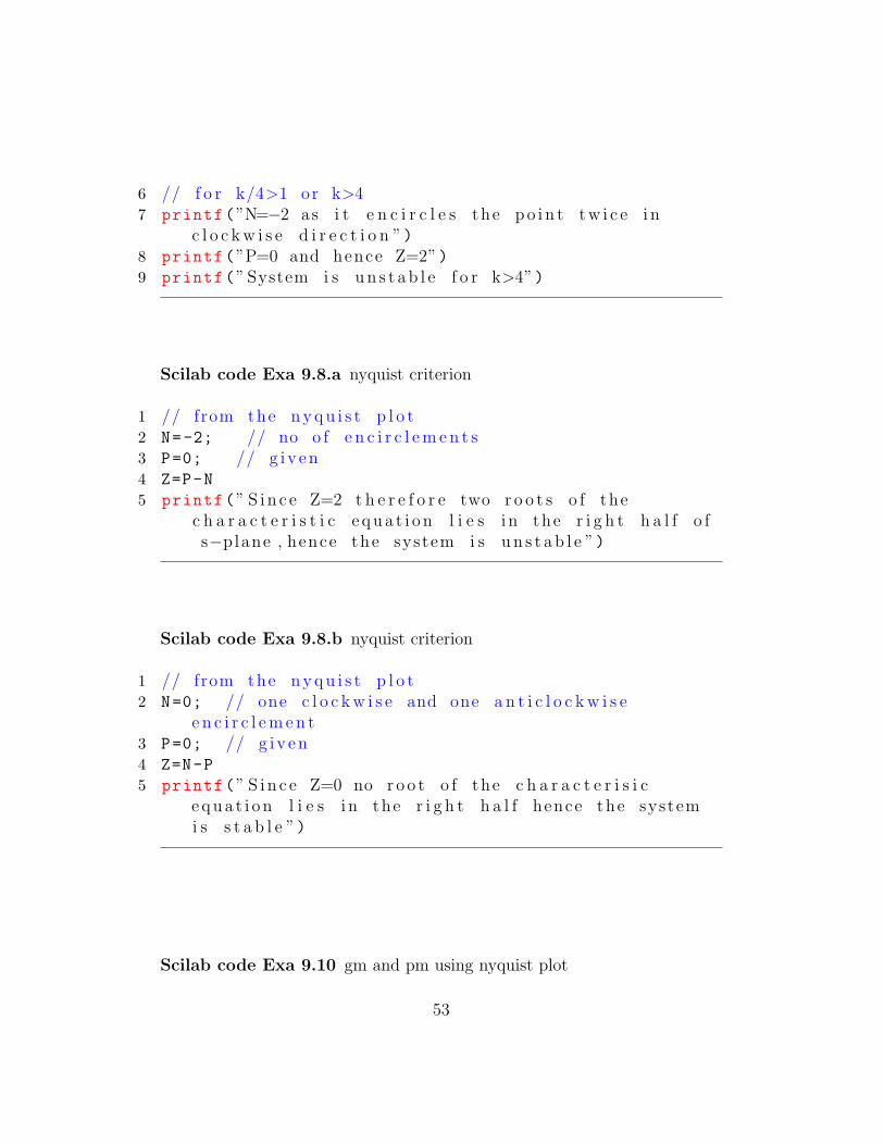
Scilab code Exa 9.10 gm and pm using nyquist plot
53
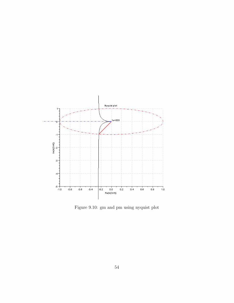
Figure 9.10: gm and pm using nyquist plot
54
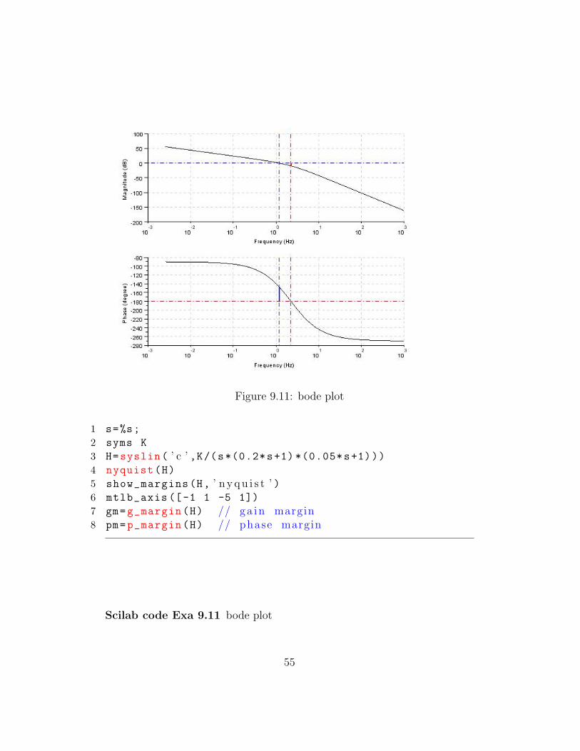
Figure 9.11: bode plot
1 s=%s;
2 syms K
3 H=syslin( ’ c ’ ,K/(s*(0.2*s+1) *(0.05*s+1)))4 nyquist(H)
5 show_margins(H, ’ n y q u i s t ’ )6 mtlb_axis ([-1 1 -5 1])
7 gm=g_margin(H) // ga in margin8 pm=p_margin(H) // phase margin
Scilab code Exa 9.11 bode plot
55
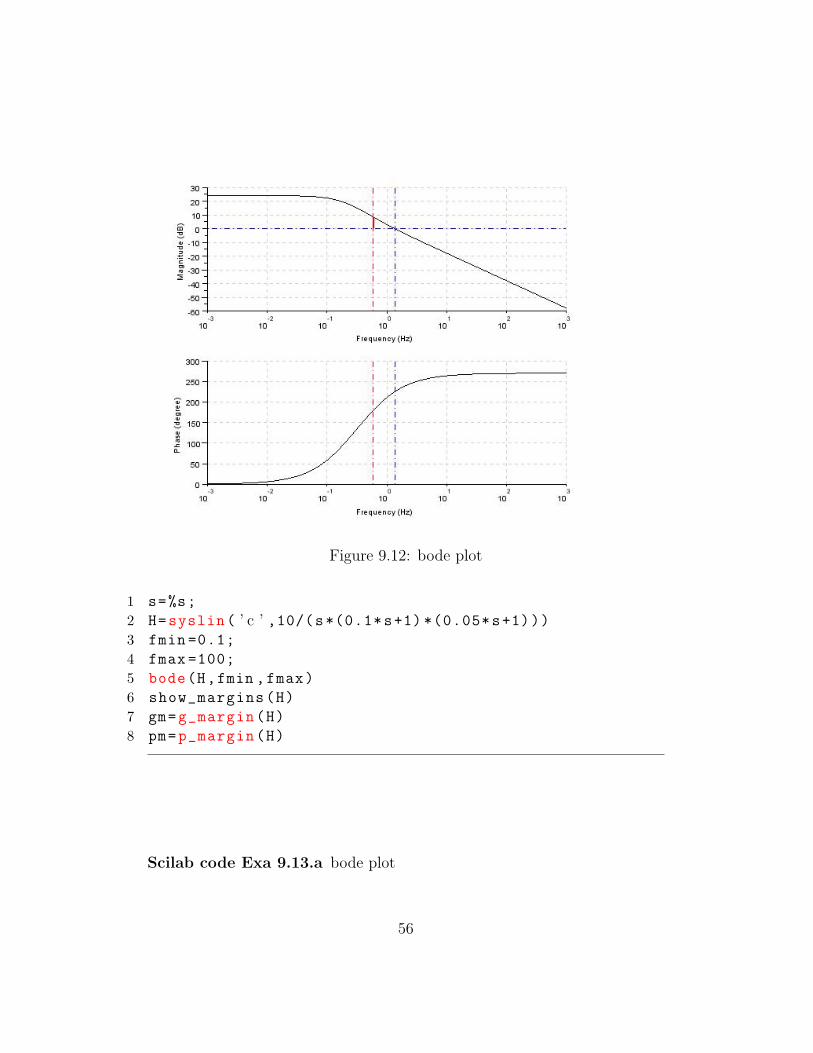
Figure 9.12: bode plot
1 s=%s;
2 H=syslin( ’ c ’ ,10/(s*(0.1*s+1) *(0.05*s+1)))3 fmin =0.1;
4 fmax =100;
5 bode(H,fmin ,fmax)
6 show_margins(H)
7 gm=g_margin(H)
8 pm=p_margin(H)
Scilab code Exa 9.13.a bode plot
56
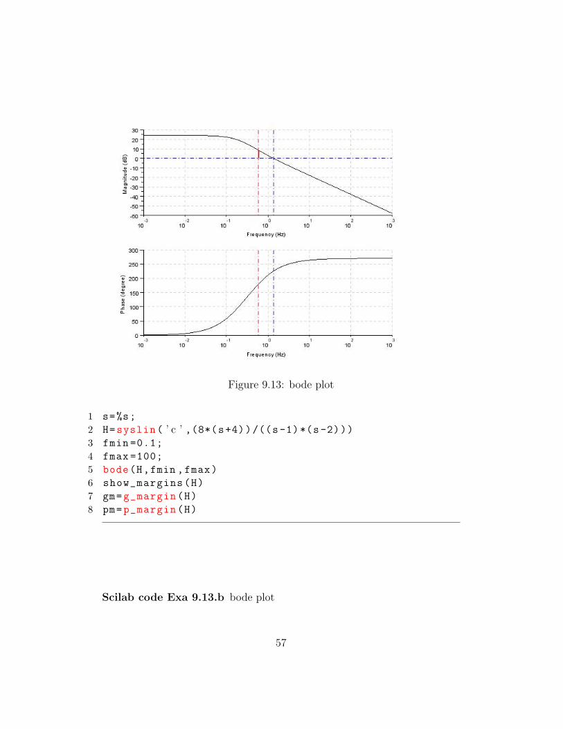
Figure 9.13: bode plot
1 s=%s;
2 H=syslin( ’ c ’ ,(8*(s+4))/((s-1)*(s-2)))3 fmin =0.1;
4 fmax =100;
5 bode(H,fmin ,fmax)
6 show_margins(H)
7 gm=g_margin(H)
8 pm=p_margin(H)
Scilab code Exa 9.13.b bode plot
57
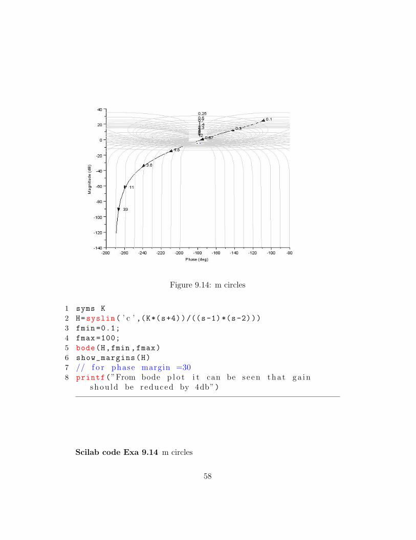
Figure 9.14: m circles
1 syms K
2 H=syslin( ’ c ’ ,(K*(s+4))/((s-1)*(s-2)))3 fmin =0.1;
4 fmax =100;
5 bode(H,fmin ,fmax)
6 show_margins(H)
7 // f o r phase margin =308 printf(”From bode p l o t i t can be s e en tha t ga in
shou ld be reduced by 4db”)
Scilab code Exa 9.14 m circles
58
1 s=%s;
2 H=syslin( ’ c ’ ,10/(s*((0.1*s)+1) *((0.5*s)+1)))3 fmin =0.1;
4 fmax =100;
5 clf()
6 black(H,0.1 ,100)
7 chart(list (1,0))
8 gm=g_margin(H)
9 pm=p_margin(H)
10 printf(” For ga in margin o f 20 db p l o t i s s h i f t e ddownwards by 8 db and a phase margin o f 24d e g r e e s i s o b t a i n e d i f cu rve i s s h i f t e d upwardsby 3 . 5 db”)
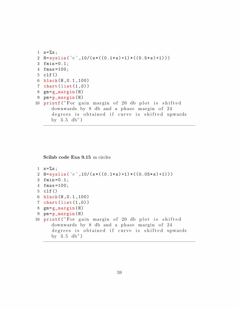
Scilab code Exa 9.15 m circles
1 s=%s;
2 H=syslin( ’ c ’ ,10/(s*((0.1*s)+1) *((0.05*s)+1)))3 fmin =0.1;
4 fmax =100;
5 clf()
6 black(H,0.1 ,100)
7 chart(list (1,0))
8 gm=g_margin(H)
9 pm=p_margin(H)
10 printf(” For ga in margin o f 20 db p l o t i s s h i f t e ddownwards by 8 db and a phase margin o f 24d e g r e e s i s o b t a i n e d i f cu rve i s s h i f t e d upwardsby 3 . 5 db”)
59
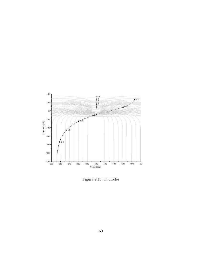
Figure 9.15: m circles
60
Chapter 10
Introduction to Design
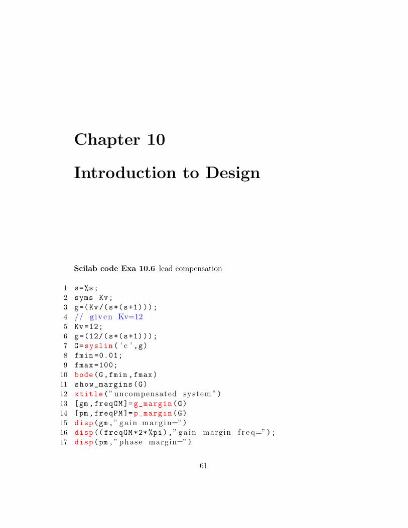
Scilab code Exa 10.6 lead compensation
1 s=%s;
2 syms Kv;
3 g=(Kv/(s*(s+1)));
4 // g i v e n Kv=125 Kv=12;
6 g=(12/(s*(s+1)));
7 G=syslin( ’ c ’ ,g)8 fmin =0.01;
9 fmax =100;
10 bode(G,fmin ,fmax)
11 show_margins(G)
12 xtitle(” uncompensated system ”)13 [gm ,freqGM ]= g_margin(G)
14 [pm ,freqPM ]= p_margin(G)
15 disp(gm,” g a i n m a r g i n=”)16 disp(( freqGM *2*%pi),” ga in margin f r e q=”);17 disp(pm,” phase margin=”)
61
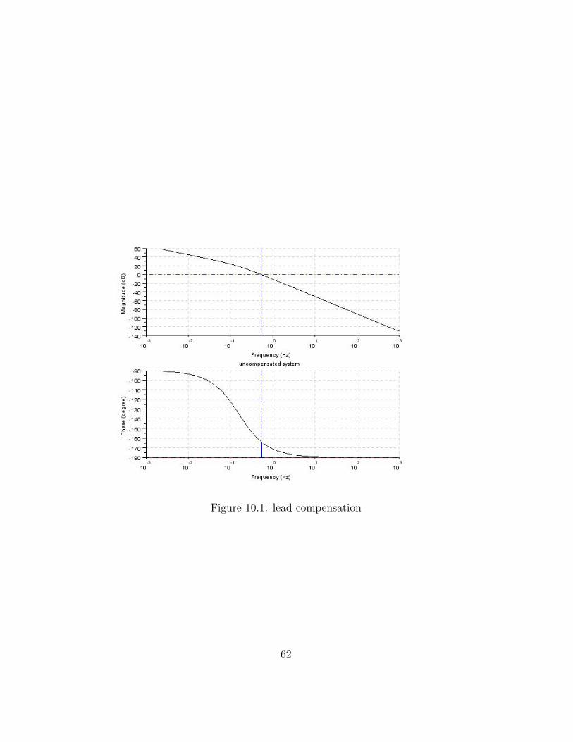
Figure 10.1: lead compensation
62
Figure 10.2: lead compensation
63
18 disp(( freqPM *2*%pi),” phase margin f r e q=”);19 printf(” s i n c e P .M i s l e s s than d e s i r e d v a l u e so we
need phase l e a d network ”)20 disp(” s e l e c t i n g z e r o o f l e a d compenst ing network at
w=2.65 rad / s e c and p o l e at w=7.8 rad / s e c anda p p l y i n g ga in to account a t t e n u a t i o n f a c t o r . ”)
21 gc =(1+0.377*s)/(1+0.128*s)
22 Gc=syslin( ’ c ’ ,gc)23 disp(Gc,” t r a n s f e r f u n c t i o n o f l e a d compensator=”);24 G1=G*Gc
25 disp(G1,” o v e r a l l t r a n s f e r f u n c t i o n=”);26 fmin =0.01;
27 fmax =100;
28 bode(G1,fmin ,fmax);
29 show_margins(G1)
30 xtitle(” compensated system ”)31 [gm ,freqGM ]= g_margin(G1);
32 [pm ,freqPM ]= p_margin(G1);
33 disp(pm,” phase margin o f compensated system=”)34 disp(( freqPM *2*%pi),” ga in c r o s s ove r f r e q u e n c y=”)
Scilab code Exa 10.7 lead compensation
1 s=%s;
2 syms Ka;
3 g=(Ka/(s^2*(1+0.2*s)));
4 // g i v e n Ka=105 Ka=10;
6 g=(10/(s^2*(1+0.2*s)));
7 G=syslin( ’ c ’ ,g)8 fmin =0.01;
64
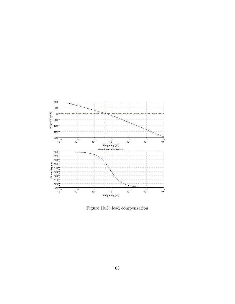
Figure 10.3: lead compensation
65
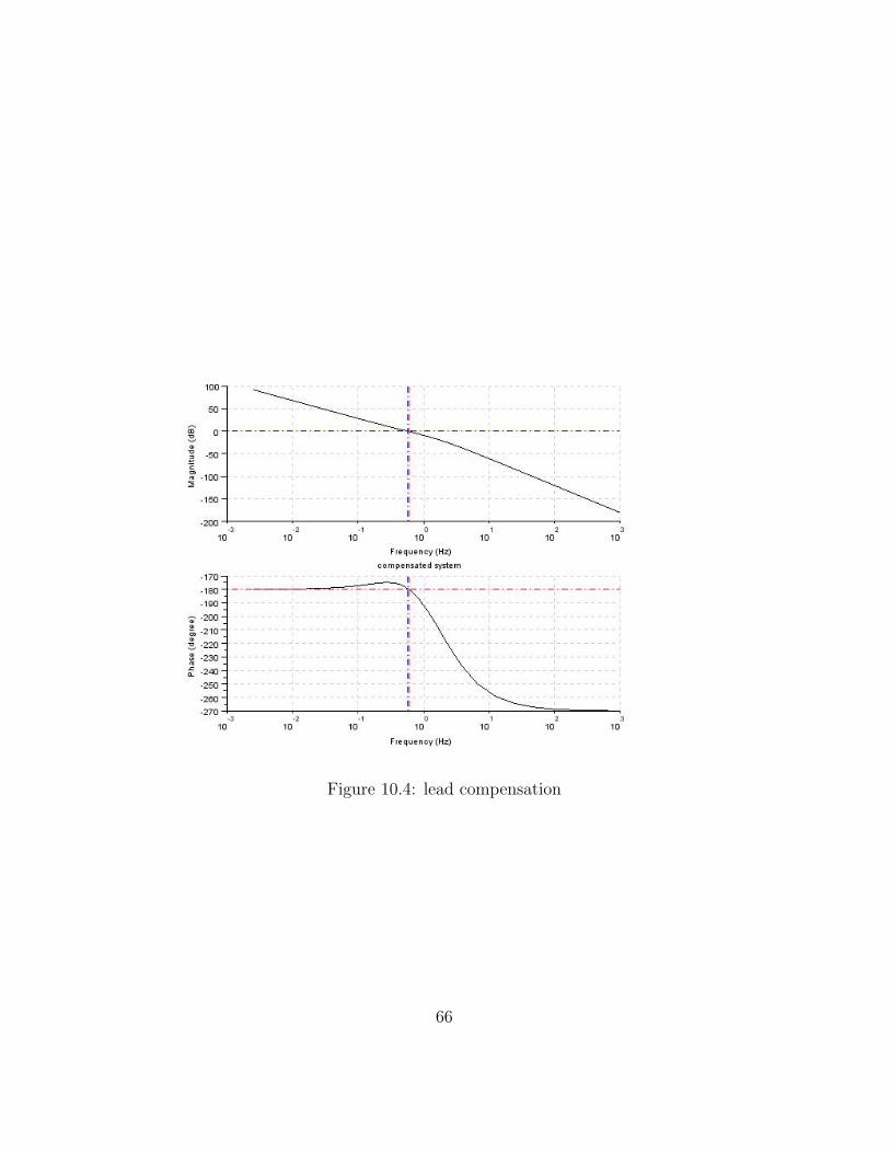
Figure 10.4: lead compensation
66
9 fmax =100;
10 bode(G,fmin ,fmax)
11 show_margins(G)
12 xtitle(” uncompensated system ”)13 [gm ,freqGM ]= g_margin(G)
14 [pm ,freqPM ]= p_margin(G)
15 disp(gm,” g a i n m a r g i n=”)16 disp(( freqGM *2*%pi),” ga in margin f r e q=”);17 disp(pm,” phase margin=”)18 disp(( freqPM *2*%pi),” phase margin f r e q=”);19 disp(” s i n c e P .M i s n e g a t i v e so system i s u n s t a b l e ”)20 disp(” s e l e c t i n g z e r o o f l e a d compensat ing network at
w=2.8 rad / s e c and p o l e at w=14 rad / s e c anda p p l y i n g ga in to account a t t e n u a t i o n f a c t o r . ”)
21 gc =(1+0.358*s)/(1+0.077*s)
22 Gc=syslin( ’ c ’ ,gc)23 disp(Gc,” t r a n s f e r f u n c t i o n o f l e a d compensator=”);24 G1=G*Gc
25 disp(G1,” o v e r a l l t r a n s f e r f u n c t i o n=”);26 fmin =0.01;
27 fmax =100;
28 bode(G1,fmin ,fmax);
29 show_margins(G1)
30 xtitle(” compensated system ”)31 [gm ,freqGM ]= g_margin(G1);
32 [pm ,freqPM ]= p_margin(G1);
33 disp(pm,” phase margin o f compensated system=”)34 disp(( freqPM *2*%pi),” ga in c r o s s ove r f r e q u e n c y=”)
Scilab code Exa 10.8 lag compnsation
67
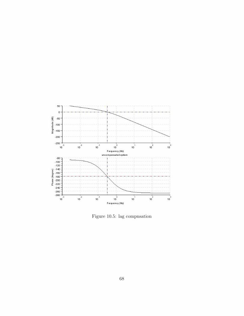
Figure 10.5: lag compnsation
68
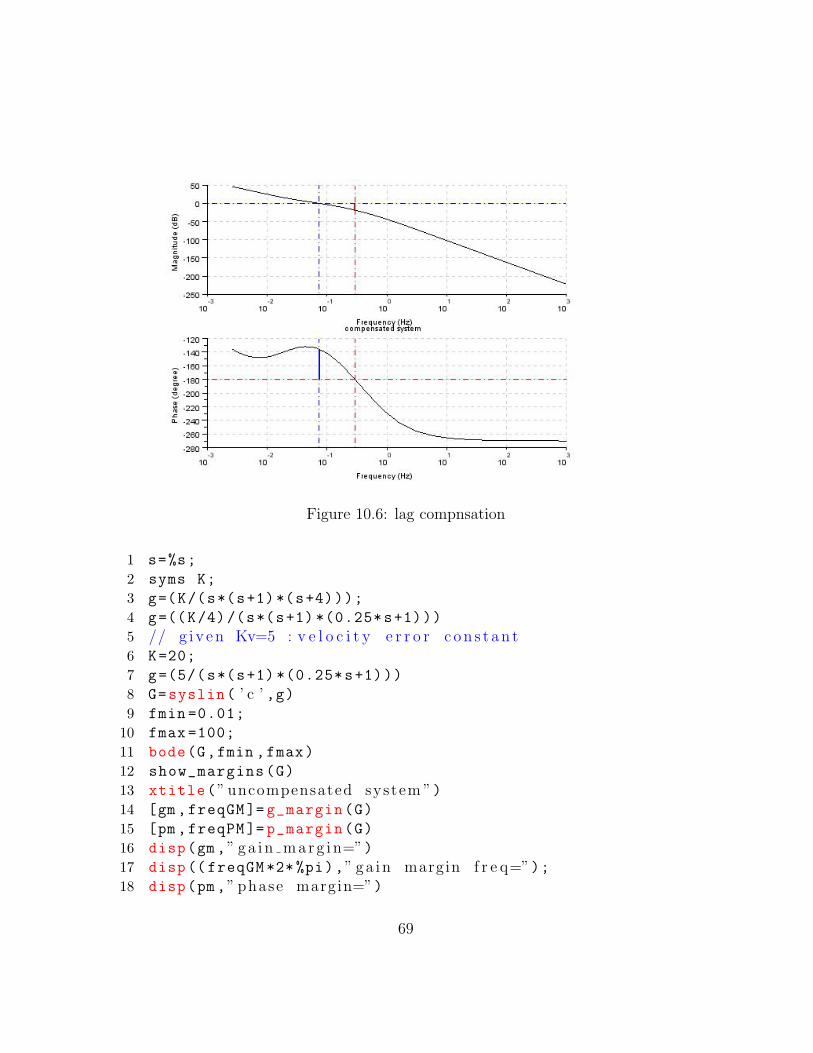
Figure 10.6: lag compnsation
1 s=%s;
2 syms K;
3 g=(K/(s*(s+1)*(s+4)));
4 g=((K/4)/(s*(s+1) *(0.25*s+1)))
5 // g i v e n Kv=5 : v e l o c i t y e r r o r c o n s t a n t6 K=20;
7 g=(5/(s*(s+1) *(0.25*s+1)))
8 G=syslin( ’ c ’ ,g)9 fmin =0.01;
10 fmax =100;
11 bode(G,fmin ,fmax)
12 show_margins(G)
13 xtitle(” uncompensated system ”)14 [gm ,freqGM ]= g_margin(G)
15 [pm ,freqPM ]= p_margin(G)
16 disp(gm,” g a i n m a r g i n=”)17 disp(( freqGM *2*%pi),” ga in margin f r e q=”);18 disp(pm,” phase margin=”)
69
19 disp(( freqPM *2*%pi),” phase margin f r e q=”);20 disp(” s i n c e P .M i s n e g a t i v e so system i s u n s t a b l e ”)21 disp(” s e l e c t i n g z e r o o f phase l a g network at w=0.013
rad / s e c and p o l e at w=0.13 rad / s e c and a p p l y i n gga in to account a t t e n u a t i o n f a c t o r ”)
22 gc=((s+0.13) /(10*(s+0.013)))
23 Gc=syslin( ’ c ’ ,gc)24 disp(Gc,” t r a n s f e r f u n c t i o n o f l a g compensator=”);25 G1=G*Gc
26 disp(G1,” o v e r a l l t r a n s f e r f u n c t i o n=”);27 fmin =0.01;
28 fmax =100;
29 bode(G1,fmin ,fmax);
30 show_margins(G1)
31 xtitle(” compensated system ”)32 [gm ,freqGM ]= g_margin(G1);
33 [pm ,freqPM ]= p_margin(G1);
34 disp(pm,” phase margin o f compensated system=”)35 disp(( freqPM *2*%pi),” ga in c r o s s ove r f r e q u e n c y=”)
Scilab code Exa 10.9 lag and lead compensation
1 s=%s;
2 syms K;
3 g=(K/(s*(0.1*s+1) *(0.2*s+1)));
4 // g i v e n Kv=30 : v e l o c i t y e r r o r c o n s t s n t5 K=30;
6 g=(30/(s*(0.1*s+1) *(0.2*s+1)))
7 G=syslin( ’ c ’ ,g)8 fmin =0.01;
9 fmax =100;
70
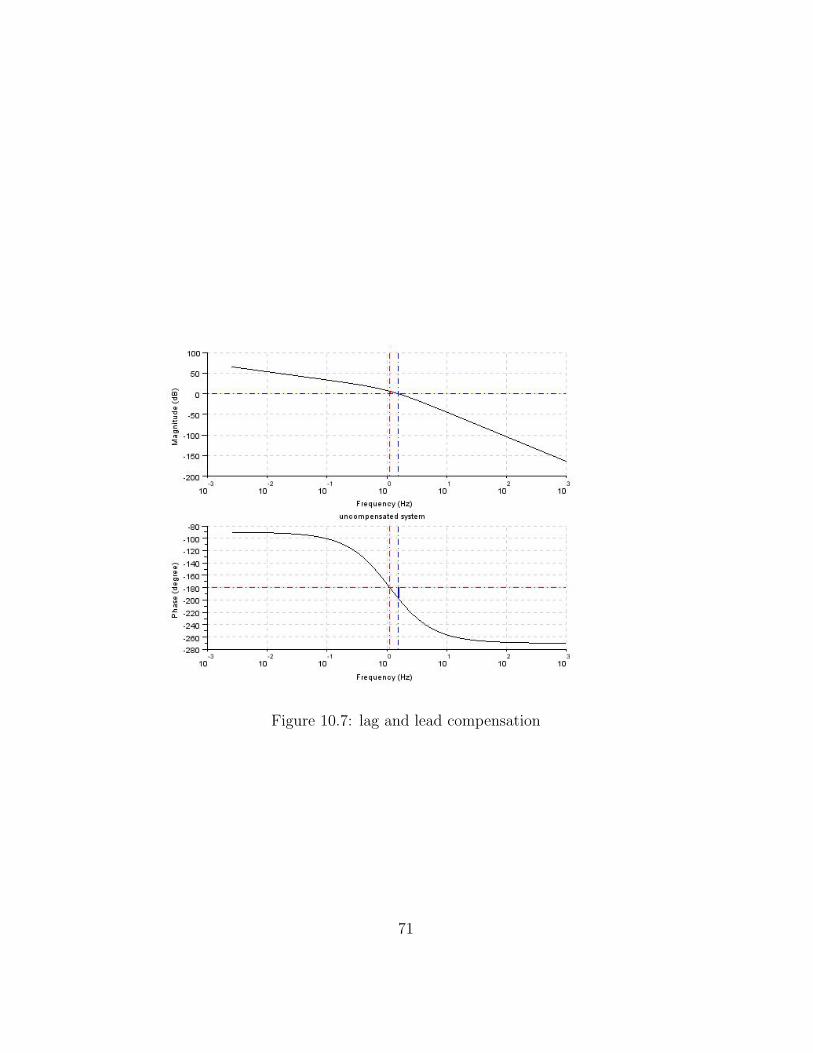
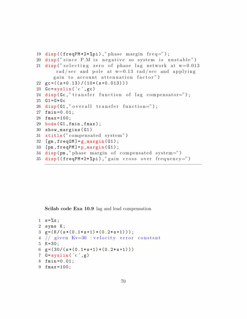
Figure 10.7: lag and lead compensation
71
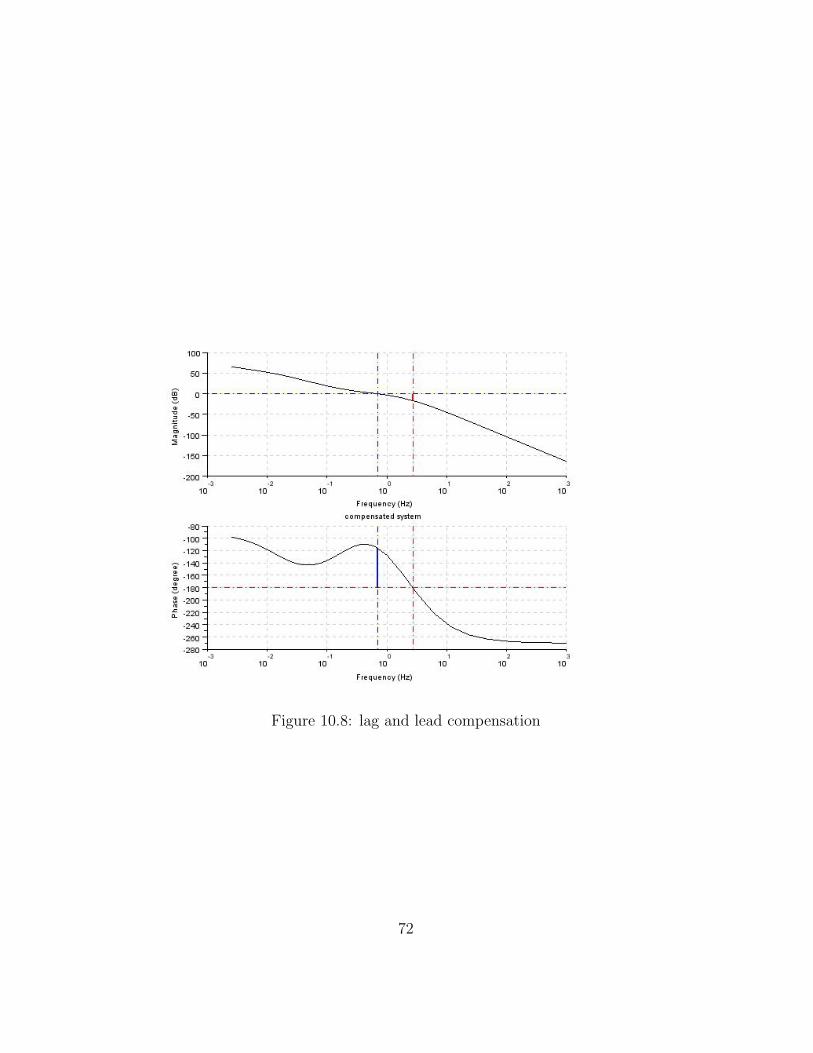
Figure 10.8: lag and lead compensation
72
10 bode(G,fmin ,fmax)
11 show_margins(G)
12 xtitle(” uncompensated system ”)13 [gm ,freqGM ]= g_margin(G)
14 [pm ,freqPM ]= p_margin(G)
15 disp(gm,” g a i n m a r g i n=”)16 disp(( freqGM *2*%pi),” ga in margin f r e q=”);17 disp(pm,” phase margin=”)18 disp(( freqPM *2*%pi),” phase margin f r e q=”);19 disp(” s i n c e P .M i s n e g a t i v e so system i s u n s t a b l e ”)20 disp(” I f l e a d compenst ion i s used bandwidth w i l l
i n c r e a s e r e s u l t i n g i n u n d e s i r a b l e systems e n s i t i v e to n o i s e . I f l a g compensat ion i s usedbandwidth d e c r e a s e s so as to f a l l s h o r t o fs p e c i f i e d v a l u e o f 12 rad / s e c r e s u l t i n g i ns l u g g i s h system ”)
21 disp(”/n hence we use a lag−l e a d compensator ”)22 // l a g compensator23 disp(” s e l e c t i n g z e r o o f phase l a g network w=1 rad /
s e c and p o l e at w=0.1 rad / s e c and a p p l y i n g ga into account a t t e n u a t i o n f a c t o r ”)
24 gc1 =((s+1) /(10*s+1));
25 Gc1=syslin( ’ c ’ ,gc1)26 disp(Gc1 ,” t r a n s f e r f u n c t i o n o f l a g compensator ”)27 // l e a d compensator28 disp(” s e l e c t i n g z e r o o f l e a d compensator at w=0.425
rad / s e c and p o l e at w=0.0425 rad / s e c ”)29 gc2 =((0.425*s+1) /(0.0425*s+1));
30 Gc2=syslin( ’ c ’ ,gc2)31 disp(Gc2 ,” t r a n s f e r f u n c t i o n o f l e a d compensator ”)32 Gc=Gc1*Gc2 // t r a n s f e r f u n c t i o n o f l a g and l e a d
s e c t i o n s33 disp(Gc,” t r a n s f e r f u n c t i o n o f l a g and l e a d s e c t i o n s ”
)
34 G1=G*Gc
35 disp(G1,” o v e r a l l t r a n s f e r f u n c t i o n=”);36 fmin =0.01;
37 fmax =100;
73
38 bode(G1,fmin ,fmax);
39 show_margins(G1)
40 xtitle(” compensated system ”)41 [gm ,freqGM ]= g_margin(G1);
42 [pm ,freqPM ]= p_margin(G1);
43 disp(pm,” phase margin o f compensated system=”)44 disp(( freqPM *2*%pi),” ga in c r o s s ove r f r e q u e n c y=”)
74
Chapter 12
State Variable Analysis andDesign
Scilab code Exa 12.3 state matrix
1 s=%s;
2 H=syslin( ’ c ’ ,(2*s^2+6*s+7) /((s+1) ^2*(s+2)))3 SS=tf2ss(H)
4 [Ac ,Bc,U,ind]=canon(SS(2),SS(3))
Scilab code Exa 12.4 modal matrix
1 syms m11 m12 m13 m21 m22 m23 m31 m32 m33 ^
2 s=%s;
3 poly(0,” l ”);4 A=[0 1 0;3 0 2;-12 -7 -6]
5 [r c]=size(A)
6 I=eye(r,c);
7 p=l*I-A;
8 q=det(p); // de t e rminant o f l i −p9 // r o o t s o f q a r e
75
10 l1=-1;
11 l2=-2;
12 l3=-3;
13 x1=[m11;m21;m31];
14 q1=(l1*I-A)*1
15 // on s o l v i n g we f i n d m11=1 m21=−1 31=−116 m11 =1;m21=-1;m31=-1;
17 x2=[m12;m22;m32];
18 q2=(l2*I-A)*1
19 // on s o l v i n g we f i n d m12=2 m22=−4 m32=120 m12 =2;m22=-4;m32 =1;
21 x3=[m13;m23;m33];
22 q3=(l3*I-A)*1
23 // on s o l v i n g we ge t m13=1 m23=−3 m33=324 m13 =1;m23=-3;m33 =3;
25 // modal matr ix i s26 M=[m11 m12 m13;m21 m22 23; m31 m32 m33]
Scilab code Exa 12.5 obtain time response
1 syms t m
2 s=%s;
3 A=[1 0;1 1];
4 B=[1;1];
5 x=[1;0];
6 [r c]=size(A)
7 p=s*eye(r,c)-A // s ∗ I−A8 q=inv(p)
9 for i=1:r
10 for j=1:c
11 // i n v e r s e l a p l a c e o f each e l ement o f Matr ix q12 q(i,j)=ilaplace(q(i,j),s,t);
13 end
14 end
15 disp(q,” ph i ( t )=”) // S t a t e T r a n s i t i o n Matr ix
76
16 t=t-m;
17 q=eval(q)
18 // I n t e g r a t e q w. r . t m19 r=integrate(q*B,m)
20 m=0 // Upper l i m i t i s t21 g=eval(r) // Put ing upper l i m i t i n q22 m=t // Lower l i m i t i s 023 h=eval(r) // Put t ing l owe r l i m i t i n q24 y=(h-g);
25 disp(y,”y=”)26 printf(”x ( t )=phi ( t ) ∗x ( 0 )+i n t e g r a t e ( ph i ( t−m∗B) w. r . t
m from 0 to t ) ”)27 y1=(q*x)+y;
28 disp(y1,”x ( t )=”)
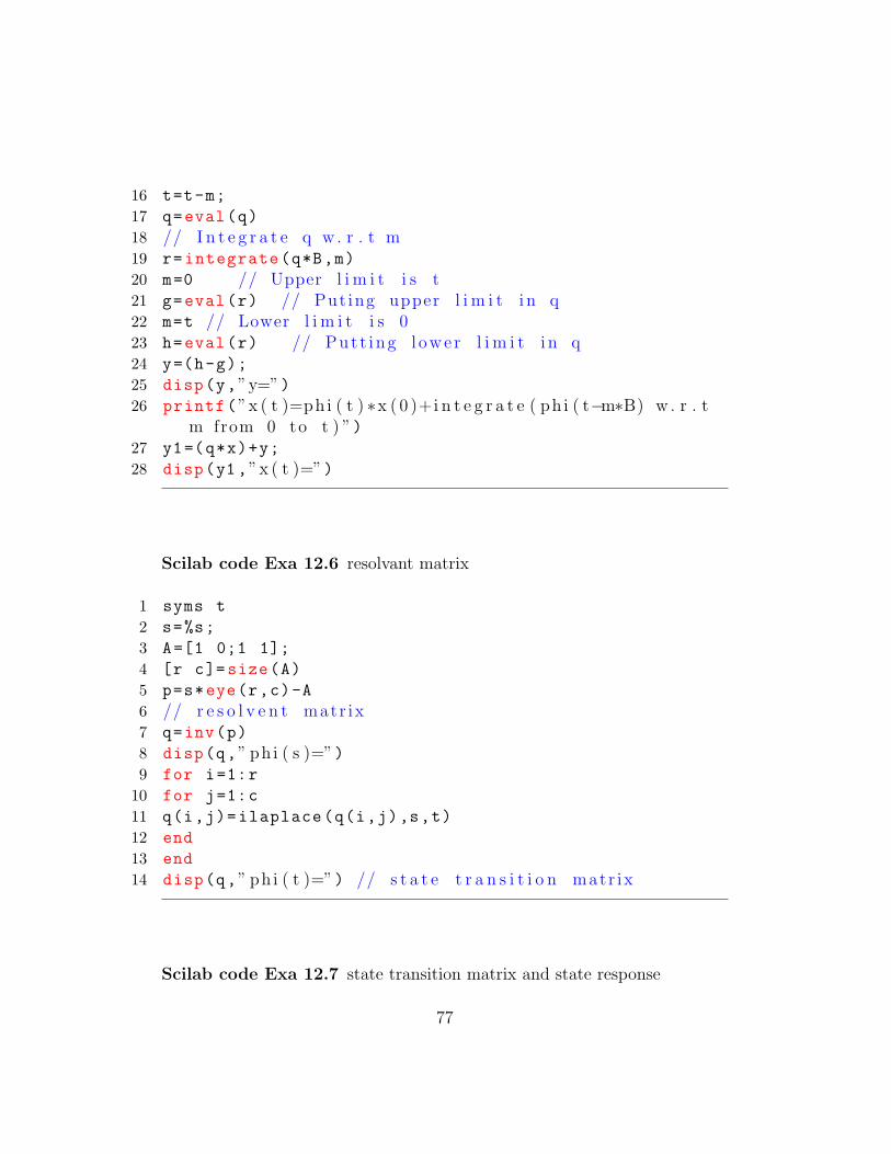
Scilab code Exa 12.6 resolvant matrix
1 syms t
2 s=%s;
3 A=[1 0;1 1];
4 [r c]=size(A)
5 p=s*eye(r,c)-A
6 // r e s o l v e n t matr ix7 q=inv(p)
8 disp(q,” ph i ( s )=”)9 for i=1:r
10 for j=1:c
11 q(i,j)=ilaplace(q(i,j),s,t)
12 end
13 end
14 disp(q,” ph i ( t )=”) // s t a t e t r a n s i t i o n matr ix
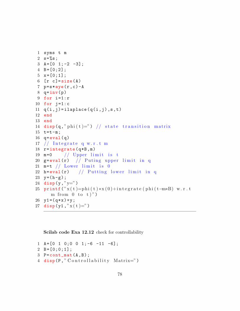
Scilab code Exa 12.7 state transition matrix and state response
77
1 syms t m
2 s=%s;
3 A=[0 1;-2 -3];
4 B=[0;2];
5 x=[0;1];
6 [r c]=size(A)
7 p=s*eye(r,c)-A
8 q=inv(p)
9 for i=1:r
10 for j=1:c
11 q(i,j)=ilaplace(q(i,j),s,t)
12 end
13 end
14 disp(q,” ph i ( t )=”) // s t a t e t r a n s i t i o n matr ix15 t=t-m;
16 q=eval(q)
17 // I n t e g r a t e q w. r . t m18 r=integrate(q*B,m)
19 m=0 // Upper l i m i t i s t20 g=eval(r) // Put ing upper l i m i t i n q21 m=t // Lower l i m i t i s 022 h=eval(r) // Put t ing l owe r l i m i t i n q23 y=(h-g);
24 disp(y,”y=”)25 printf(”x ( t )=phi ( t ) ∗x ( 0 )+i n t e g r a t e ( ph i ( t−m∗B) w. r . t
m from 0 to t ) ”)26 y1=(q*x)+y;
27 disp(y1,”x ( t )=”)
Scilab code Exa 12.12 check for controllability
1 A=[0 1 0;0 0 1;-6 -11 -6];
2 B=[0;0;1];
3 P=cont_mat(A,B);
4 disp(P,” C o n t r o l l a b i l i t y Matr ix=”)
78
5 d=det(P)
6 if d==0
7 printf(” matr ix i s s i n g u l a r , so system i su n c o n t r o l l a b l e ”);
8 else
9 printf(” system i s c o n t r o l l a b l e ”);10 end;
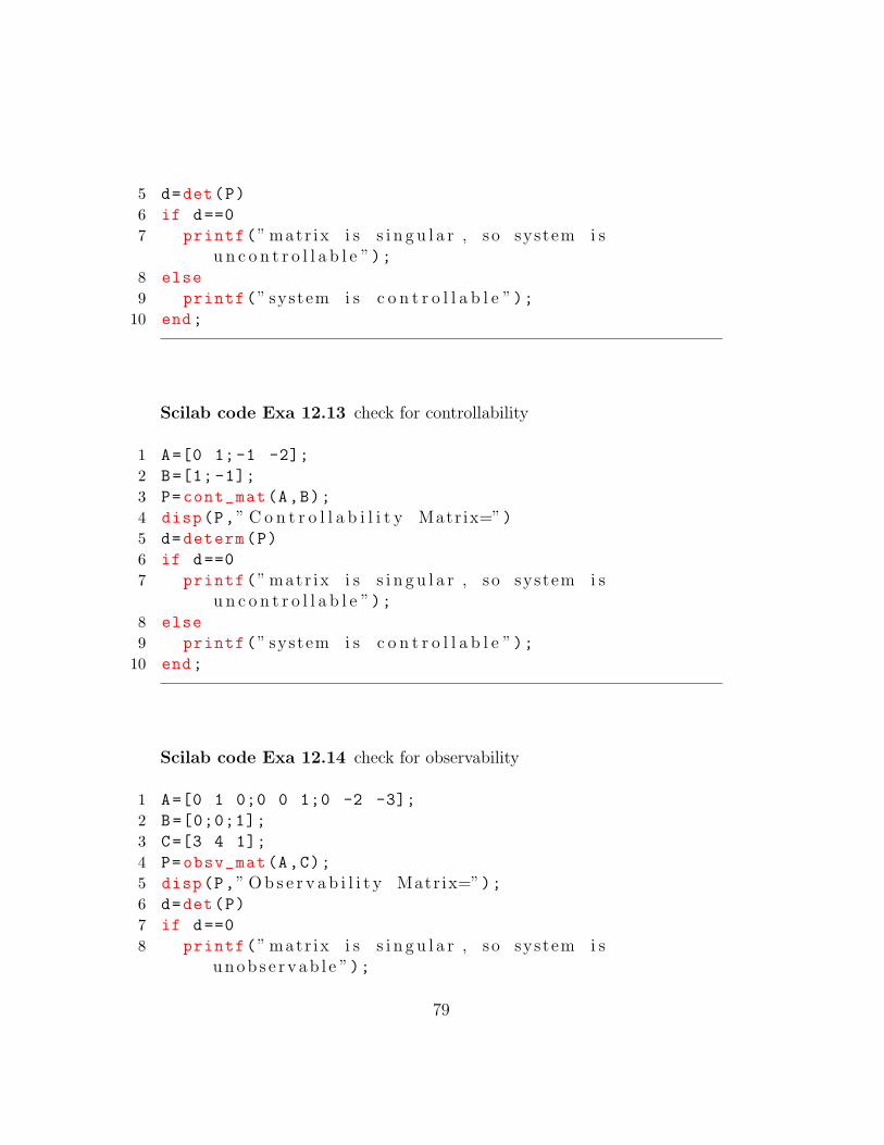
Scilab code Exa 12.13 check for controllability
1 A=[0 1;-1 -2];
2 B=[1; -1];
3 P=cont_mat(A,B);
4 disp(P,” C o n t r o l l a b i l i t y Matr ix=”)5 d=determ(P)
6 if d==0
7 printf(” matr ix i s s i n g u l a r , so system i su n c o n t r o l l a b l e ”);
8 else
9 printf(” system i s c o n t r o l l a b l e ”);10 end;
Scilab code Exa 12.14 check for observability
1 A=[0 1 0;0 0 1;0 -2 -3];
2 B=[0;0;1];
3 C=[3 4 1];
4 P=obsv_mat(A,C);
5 disp(P,” O b s e r v a b i l i t y Matr ix=”);6 d=det(P)
7 if d==0
8 printf(” matr ix i s s i n g u l a r , so system i su n o b s e r v a b l e ”);
79
9 else
10 printf(” system i s o b s e r v a b l e ”);11 end;
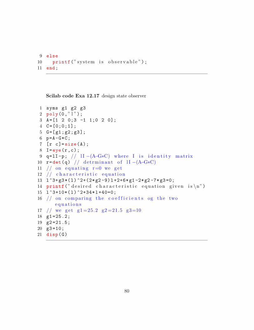
Scilab code Exa 12.17 design state observer
1 syms g1 g2 g3
2 poly(0,” l ”);3 A=[1 2 0;3 -1 1;0 2 0];
4 C=[0;0;1];
5 G=[g1;g2;g3];
6 p=A-G*C;
7 [r c]=size(A);
8 I=eye(r,c);
9 q=lI -p; // l I −(A−G∗C) where I i s i d e n t i t y matr ix10 r=det(q) // det rminant o f l I −(A−G∗C)11 // on e q u a t i n g r=0 we g e t12 // c h a r a c t e r i s t i c e q u a t i o n13 l^3+g3*(l)^2+(2*g2 -9)l+2+6*g1 -2*g2 -7*g3=0;
14 printf(” d e s i r e d c h a r a c t e r i s t i c e q u a t i o n g i v e n i s \n”)15 l^3+10*(l)^2+34*l+40=0;
16 // on comparing the c o e f f i c i e n t s og the twoe q u a t i o n s
17 // we g e t g1 =25.2 g2 =21.5 g3=1018 g1 =25.2;
19 g2 =21.5;
20 g3=10;
21 disp(G)
80
Recommended