NBER WORKING PAPER SERIES
COMMUTING, MIGRATION AND LOCAL EMPLOYMENT ELASTICITIES
Ferdinando MonteStephen J. Redding
Esteban Rossi-Hansberg
Working Paper 21706http://www.nber.org/papers/w21706
NATIONAL BUREAU OF ECONOMIC RESEARCH1050 Massachusetts Avenue
Cambridge, MA 02138November 2015
Much of this research was undertaken while Ferdinando Monte was visiting the International EconomicsSection (IES) at Princeton. We are grateful to the IES and Princeton more generally for research support.We are also grateful to the editor, four anonymous referees, and conference and seminar participantsfor helpful comments and suggestions. The views expressed herein are those of the authors and donot necessarily reflect the views of the National Bureau of Economic Research.
NBER working papers are circulated for discussion and comment purposes. They have not been peer-reviewed or been subject to the review by the NBER Board of Directors that accompanies officialNBER publications.
© 2015 by Ferdinando Monte, Stephen J. Redding, and Esteban Rossi-Hansberg. All rights reserved.Short sections of text, not to exceed two paragraphs, may be quoted without explicit permission providedthat full credit, including © notice, is given to the source.

Commuting, Migration and Local Employment ElasticitiesFerdinando Monte, Stephen J. Redding, and Esteban Rossi-HansbergNBER Working Paper No. 21706November 2015, Revised November 2016JEL No. F16,J6,J61,R0
ABSTRACT
To understand the elasticity of employment to local labor demand shocks, we develop a quantitativegeneral equilibrium model that incorporates spatial linkages in goods markets (trade) and factor markets(commuting and migration). We show that local employment elasticities differ substantially acrossU.S. counties and commuting zones in ways that are not well explained by standard empirical controlsbut are captured by commuting measures. We provide independent evidence for these predictionsfrom million dollar plants and find that empirically-observed reductions in commuting costs generatewelfare gains of around 3.3 percent and employment reallocations from -20 to 30 percent.
Ferdinando MonteGeorgetown UniversityMcDonough School of Business37th & O Streets, NWWashington, DC [email protected]
Stephen J. ReddingDepartment of Economicsand Woodrow Wilson SchoolPrinceton UniversityFisher HallPrinceton, NJ 08544and [email protected]
Esteban Rossi-HansbergPrinceton UniversityDepartment of EconomicsFisher HallPrinceton, NJ 08544-1021and [email protected]

Commuting, Migration and Local EmploymentElasticities∗
Ferdinando Monte†
Georgetown University
Stephen J. Redding‡
Princeton University
Esteban Rossi-Hansberg§
Princeton University
October 30, 2016
Abstract
To understand the elasticity of employment to local labor demand shocks, we develop a quantita-tive general equilibrium model that incorporates spatial linkages in goods markets (trade) and factormarkets (commuting and migration). We show that local employment elasticities differ substantiallyacross U.S. counties and commuting zones in ways that are not well explained by standard empiricalcontrols but are captured by commuting measures. We provide independent evidence for these pre-dictions from million dollar plants and find that empirically-observed reductions in commuting costsgenerate welfare gains of around 3.3 percent and employment reallocations from -20 to 30 percent.
JEL CLASSIFICATION: F12, F14, R13, R23
1 Introduction
Agents spend about 8% of their workday commuting to and from work.1 They make this significantdaily investment, to live and work in different locations, so as to balance their living costs and residentialamenities with the wage they can obtain at their place of employment. The ability of firms in a location toattract workers depends, therefore, not only on the ability to attract local residents through migration, butalso on the ability to attract commuters from other, nearby, locations. Together, migration and commut-ing determine the response of local employment to a local labor demand shock, which we term the local
employment elasticity. This elasticity is of great policy interest since it determines the impact of localpolicies, such as transport infrastructure investments, local taxation and regional development programs.Estimating its magnitude has been the subject of a large empirical literature on local labor markets, which
∗Much of this research was undertaken while Ferdinando Monte was visiting the International Economics Section (IES) atPrinceton. We are grateful to the IES and Princeton more generally for research support. We are also grateful to the editor, fouranonymous referees, and conference and seminar participants for helpful comments and suggestions.†McDonough School of Business, 37th and O Streets, NW, Washington, DC 20057. [email protected].‡Dept. Economics and WWS, Fisher Hall, Princeton, NJ 08544. 609 258 4016. [email protected].§Dept. Economics and WWS, Fisher Hall, Princeton, NJ 08544. 609 258 4024. [email protected] for example Redding and Turner (2015).
1

has considered a variety of sources of local labor demand shocks, including sectoral composition (Bartikshocks), productivity, international trade, natural resource abundance and business cycle fluctuations, asdiscussed further below.2 In this paper we explore the determinants and characteristics of the local em-ployment elasticity (and the corresponding local resident elasticity) using a detailed quantitative spatialequilibrium theory.
We develop a quantitative spatial general equilibrium model that incorporates spatial linkages betweenlocations in both goods markets (trade) and factor markets (commuting and migration). We show that thereis no single local employment elasticity. Instead the local employment elasticity is an endogenous variablethat differs across locations depending on their linkages to one another in goods and factor markets. Cali-brating our model to county-level data for the United States, we find that the elasticity of local employmentwith respect to local productivity shocks varies from around 0.5 to 2.5. Therefore an average local employ-ment elasticity estimated from cross-section data can be quite misleading when used to predict the impactof a local shock on any individual county and can lead to substantial under or overprediction of the effectof the shock. We use our quantitative model to understand the systematic determinants of the local em-ployment elasticity and show that a large part of the variation results from differences in commuting linksbetween a location and its neighbors. We then propose variables that can be included in reduced-formregressions to improve their ability to predict the heterogeneity in local employment responses withoutimposing the full structure of our model.
Our theoretical framework allows for an arbitrary number of locations that can differ in productivity,amenities and geographical relationship to one another. The spatial distribution of economic activity isdriven by a tension between productivity differences and home market effects (forces for the concentrationof economic activity) and an inelastic supply of land and commuting costs (dispersion forces). Commutingallows workers to access high productivity employment locations without having to live there and hencealleviates the congestion effect in such high productivity locations. We show that the resulting commutingflows between locations exhibit a gravity equation relationship with a much higher distance elasticitythan for goods flows, suggesting that moving people is more costly than moving goods across geographicspace. We discipline our quantitative spatial model to match the observed gravity equation relationshipsfor trade in goods and commuting flows as well as the observed cross-section distributions of employment,residents and wages across U.S. counties. Given the observed data on wages, employment by workplace,commuting flows and land area, and a parameterization of trade and commuting costs, we show that ourmodel can be used to recover unique values of the unobserved location fundamentals (productivity andamenities) that exactly rationalize the observed data as an equilibrium of the model. We show how thevalues of these observed variables in an initial equilibrium can be used to undertake counterfactuals for theimpact of local labor demand shocks (captured by productivity shocks in our model) and for the impact ofchanges in trade or commuting costs.
An advantage of our explicitly modeling the spatial linkages between locations is that our frameworkcan be taken to data on local economic activity at different levels of spatial aggregation. In contrast,
2For a survey of this empirical literature, see Moretti (2011).
2
existing research that does not explicitly model the spatial linkages between locations is faced with atrade-off when studying local labor markets. On the one hand, larger spatial units have the advantageof reducing the unmodeled spatial linkages between locations. On the other hand, larger spatial unitshave the disadvantage of reducing the ability to make inferences about local labor markets. Furthermore,there exists no choice of boundaries that eliminates commuting between spatial units. For example, shouldPrinceton, NJ be considered part of New York’s or Philadelphia’s local labor market? Some of its residentscommute to New York, but others commute to Philadelphia. Our approach overcomes these problems byexplicitly modeling the geographic linkages between the spatial units. In our baseline specification, wereport results for counties, because this is the finest level of geographical detail at which commuting dataare reported in the American Community Survey and Decennial Census, and several influential papers inthe local labor markets literature have used county data (such as Greenstone, Hornbeck and Moretti, 2010,henceforth GHM, 2010).3 In robustness tests, we also report results for commuting zones (CZs), which areaggregations of counties by the U.S. Department of Agriculture designed to minimize commuting flowsbetween locations.
We demonstrate both theoretically and empirically the robustness of our findings of heterogeneouslocal employment elasticities. From a theoretical perspective, we show that heterogeneous local employ-ment elasticities are not specific to our theoretical model, but rather are a more generic prediction of anentire class of theoretical models consistent with a gravity equation for commuting flows. This predictionholds across a range of different versions of our model, including incorporating heterogeneous land supplyelasticities across locations, non-traded goods, congestion in commuting costs, heterogeneity in effectiveunits of labor rather than in amenities, and different assumptions about the ownership of land. These dif-ferent theoretical specifications can affect the elasticity of wages with respect to productivity, but as longas these specifications yield a gravity equation for commuting flows, they imply the same elasticity ofemployment with respect to wages. This elasticity can be derived directly from the gravity equation forcommuting flows, which we show to be a strong empirical feature of the data.
From an empirical perspective, we show that we continue to find substantial heterogeneity in theselocal employment elasticities when we incorporate the variable land supply elasticities from Saiz (2010).Introducing this second source of heterogeneity generates more variation in local resident elasticities butdoes not reduce the variation in local employment elasticities. Furthermore, we continue to find substantialdifferences between local employment and local residents elasticities, where the only reason that these twoelasticities can differ from one another is commuting. We also continue to find substantial heterogeneityin local employment elasticities when we replicate our analysis for CZs rather than counties. The reason isthat there are substantial differences across CZs in the extent to which they capture commuting links in ageographic area, and it is these differences that generate the heterogeneity in local employment elasticities.
To provide further evidence of heterogeneous local employment elasticities without using the structureof our model, we use the natural experiment of million dollar plants (MDP) from GHM (2010), one of
3The LEHD Origin-Destination Employment Statistics (LODES) reports commuting data for more disaggregated spatialunits than counties, but there is substantial interpolation, and data are missing for some state-year combinations.
3

the most influential papers in the local labor markets literature. We compare “winner” and “runner-up”counties that are similar to one another, except that the winner counties were ultimately successful inattracting a MDP. We confirm the findings of a positive average treatment effect of MDPs from GHM(2010). Additionally, we find that this average treatment effect masks considerable heterogeneity acrosscounties, which takes exactly the form predicted by our model. We find that winner counties that aremore open in commuting linkages experience substantially and statistically significantly larger increasesin employment than other winner counties.4 To provide additional independent evidence in support ofthe mechanism in our model, we also show that changes in net commuting accounted for a substantialproportion of the observed changes in employment from 1990-2010, with substantial heterogeneity acrosscounties in this relative contribution from commuting.
Having established the importance of commuting for local employment responses to local labor de-mand shocks, we next show that our model provides a platform for evaluating the counterfactual effectsof changes in trade and commuting costs. Building on approaches in the international trade literature (e.g.Head and Ries, 2001), we show how observed data on commuting flows over time can be used to back outthe empirical distribution of implied changes in commuting costs. We use this empirical distribution toundertake counterfactuals for empirically-plausible changes in commuting costs. For example, reducingcommuting costs by the median reduction from 1990-2010 (a reduction of 12 percent), we find an increasein welfare of 3.3 percent. The commuting technology facilitates a separation of workplace and residence,enabling people to work in high productivity locations and live in high amenity locations. Therefore re-ducing commuting costs increases the concentration of employment in locations that were net importers ofcommuters in the initial equilibrium (e.g. Manhattan) and enhances the clustering of residents in locationsthat initially were net exporters of commuters (e.g. parts of New Jersey). This logic seems to suggest thatcommuting might be important only for larger cities in the U.S., but this is in fact not the case. Althoughthe changes in employment as a result of eliminating commuting are well explained by initial commutingintensity, this intensity cannot be easily proxied for using standard empirical controls, such as land area,size or housing supply elasticities. These results again underscore the relevant information embedded incommuting links.
Our paper is related to several existing literatures. In international trade, our work relates to quantita-tive models of costly trade in goods following Eaton and Kortum (2002) and extensions. Our research alsocontributes to the economic geography literature on costly trade in goods and factor mobility, which typi-cally uses variation across regions or systems of cities, including Krugman (1991), Hanson (1996, 2005),Helpman (1998), Fujita et al. (1999), Rossi-Hansberg (2005), Redding and Sturm (2008), Moretti andKlein (2014), Allen and Arkolakis (2014), Caliendo, et al. (2014), Desmet and Rossi-Hansberg (2014)and Redding (2016). Our work also contributes to the urban economics literature on the costly move-ment of people (commuting), which typically uses variation within cities, including Alonso (1964), Mills(1967), Muth (1969), Lucas and Rossi-Hansberg (2002), Desmet and Rossi-Hansberg (2013), Behrens,
4These results are consistent with the empirical findings, in another context, of Manning and Petrongolo (2011), whichshows that local development policies are fairly ineffective in raising local unemployment outflows, because labor marketsoverlap, and the associated ripple effects in applications largely dilute the impact of local stimulus across space.
4

et al. (2014), Ahlfeldt, et al. (2015), Allen, Arkolakis and Li (2015) and Monte (2016). In contrast, wedevelop a framework in which an arbitrary set of regions are connected in both goods markets (throughcostly trade) and labor markets (through migration and commuting), and which encompasses both withinand across-city interactions. Although incorporating costly goods trade and commuting is a natural idea,our first main contribution is to develop a tractable framework that is amenable to both analytic and quan-titative analysis, and for which we provide general results for the existence and uniqueness of the spatialequilibrium. Our second main contribution is to quantify this framework using disaggregated data ontrade and commuting for the United States and to show how it provides a platform for evaluating a rangeof counterfactual interventions. Our third main contribution is to establish the importance of spatial inter-actions between locations (in particular through commuting) in determining the local economic effects oflocal labor demand shocks.
Our paper is also related to the large empirical literature on local labor markets, which has estimatedthe effects of local labor demand shocks: (a) GHM (2010)’s analysis of million dollar plants; (b) Autor,Dorn and Hanson (2013), which examines the local economic effects from the international trade shockprovided by China’s emergence into global markets; (c) the many empirical studies that use the Bartik(1991) instrument, which interacts aggregate industry shocks with locations’ industry employment shares,including Diamond (2016) and Notowidigdo (2013); (d) research on the geographic incidence of macroe-conomic shocks, such as the 2008 Financial Crisis and Great Recession, including Mian and Sufi (2014)and Yagan (2016); and (e) work on the impact of natural resource discoveries on the spatial distribution ofeconomic activity, as in Michaels (2011) and Feyrer, Mansur and Sacerdote (2015).5 Each of these papersis concerned with evaluating the local impact of economic shocks using data on finely-detailed spatialunits. However, these spatial units are typically treated as independent observations in reduced-form re-gressions, with little attention paid to the linkages between these spatial units in goods and labor markets,and hence with little consideration of the distinction between employment and residents introduced byendogenous commuting decisions. A key contribution of our paper is to show that understanding thesespatial linkages is central to evaluating the local impact of these and other economic shocks.
The remainder of the paper is structured as follows. Section 2 develops our theoretical framework.Section 3 discusses the quantification of the model using U.S. data and reports summary statistics oncommuting between counties. Section 4 shows both theoretically and empirically the heterogeneity oflocal employment elasticities. Section 5 studies the effect of changes in commuting costs and Section 6summarizes our conclusions. A web appendix contains the derivations of theoretical results, the proofs ofpropositions, additional robustness tests, and a description of the data sources and manipulations.
5Other related research on local labor demand shocks includes Blanchard and Katz (1992), Bound and Holzer (2000), andBusso, Gregory and Kline (2013).
5
2 The Model
We develop a spatial general equilibrium model in which locations are linked in goods markets throughtrade and in factor markets through migration and commuting. The economy consists of a set of locationsn, i ∈ N . Each location n is endowed with a supply of land (Hn). Following the new economic geogra-phy literature, we begin by interpreting land as geographical land area, which is necessarily in perfectlyinelastic supply. We later extend our analysis to interpret land as developed land area, which has a posi-tive supply elasticity that we allow to differ across locations. The economy as a whole is populated by ameasure L of workers, each of whom is endowed with one unit of labor that is supplied inelastically.
2.1 Preferences and Endowments
Workers are geographically mobile and have heterogeneous preferences for locations. Each worker choosesa pair of residence and workplace locations to maximize their utility taking as given the choices of otherfirms and workers.6 The preferences of a worker ω who lives and consumes in location n and works inlocation i are defined over final goods consumption (Cnω), residential land use (Hnω), an idiosyncraticamenities shock (bniω) and commuting costs (κni), according to the Cobb-Douglas form,7
Uniω =bniωκni
(Cnωα
)α(Hnω
1− α
)1−α
, (1)
where κni ∈ [1,∞) is an iceberg commuting cost in terms of utility.8 The idiosyncratic amenities shock(bniω) captures the idea that individual workers can have idiosyncratic reasons for living and working indifferent locations. We model this heterogeneity in amenities following McFadden (1974) and Eaton andKortum (2002).9 For each worker ω living in location n and working in location i, idiosyncratic amenities(bniω) are drawn from an independent Frechet distribution,
Gni(b) = e−Bnib−ε, Bni > 0, ε > 1, (2)
where the scale parameter Bni determines the average amenities from living in location n and working inlocation i, and the shape parameter ε > 1 controls the dispersion of amenities. This idiosyncratic amenitiesshock implies that different workers make different choices about their workplace and residence locations
6Throughout the following, we use n to denote a worker’s location of residence and consumption and i to denote a worker’slocation of employment and production, unless otherwise indicated.
7For empirical evidence using U.S. data in support of the constant housing expenditure share implied by the Cobb-Douglasfunctional form, see Davis and Ortalo-Magne (2011).
8Although we model commuting costs in terms of utility, they enter the indirect utility function multiplicatively with thewage, which implies that they are proportional to the opportunity cost of time. Therefore, similar results hold if commutingcosts are instead modeled as a reduction in effective units of labor, as discussed in Subsection B.15 of the web appendix.
9A long line of research models location decisions using preference heterogeneity, as in Artuc, Chaudhuri and McClaren(2010), Kennan and Walker (2011), Grogger and Hanson (2011), Moretti (2011) and Busso, Gregory and Kline (2013). Mod-eling individual heterogeneity in terms of productivity rather than preferences results in a similar specification, as discussed inSection B.14 of the web appendix.
6
when faced with the same prices and wages. All workers ω residing in location n and working in locationi receive the same wage and make the same consumption and residential land choices. Hence we suppressthe implicit dependence on ω except where important.10
To isolate the implications of introducing commuting, we model goods consumption as in the neweconomic geography literature. The goods consumption index in location n is a constant elasticity of sub-stitution (CES) function of consumption of a continuum of tradable varieties sourced from each locationi,
Cn =
[∑i∈N
∫ Mi
0
cni(j)ρdj
] 1ρ
, σ =1
1− ρ> 1. (3)
Utility maximization implies that equilibrium consumption in location n of each variety sourced fromlocation i is given by cni(j) = αXnP
σ−1n pni (j)
−σ, where Xn is aggregate expenditure in location n; Pnis the price index dual to (3), and pni (j) is the “cost inclusive of freight” price of a variety produced inlocation i and consumed in location n.11
Utility maximization also implies that a fraction (1−α) of worker income is spent on residential land.We assume that this land is owned by immobile landlords, who receive worker expenditure on residentialland as income, and consume only goods where they live. This assumption allows us to incorporate generalequilibrium effects from changes in the value of land, without introducing a mechanical externality intoworkers’ location decisions from the local redistribution of land rents.12 Using this assumption, totalexpenditure on consumption goods equals the fraction α of the total income of residents plus the entireincome of landlords (which equals the fraction (1− α) of the total income of residents):
PnCn = αvnRn + (1− α) vnRn = vnRn (4)
where vn is the average labor income of residents across employment locations; and Rn is the measure ofresidents. Land market clearing determines the land price (Qn) as a function of the supply of land (Hn):
Qn = (1− α)vnRn
Hn
. (5)
10Our baseline specification focuses on a single worker type with a Frechet distribution of idiosyncratic preferences fortractability, which results in similar choice probabilities to the logit model. In Subsection B.9 of the web appendix, we generalizeour analysis to multiple worker types z with different Frechet scale and shape parameters, which results in similar choiceprobabilities to the mixed logit model of McFadden and Train (2000).
11In Subsection B.11 of the web appendix, we show how this standard specification can be further generalized to introducenon-traded consumption goods.
12In Subsection B.12 of the web appendix, we show that the model has similar properties if landlords consume both con-sumption goods and residential land, although expressions are less elegant. In the web appendix, we also report the results of arobustness test, in which we instead assume that land is partially owned locally and partially owned by a national portfolio thatredistributes land rents to workers throughout the economy (as in Caliendo et al. 2014).
7

2.2 Production
Again to isolate the implications of introducing commuting, we also model production as in the new eco-nomic geography literature. Tradeable varieties are produced using labor under monopolistic competitionand increasing returns to scale. To produce a variety, a firm must incur a fixed cost of F and a constantvariable cost that depends on a location’s productivity Ai.13 Therefore the total amount of labor (li(j))required to produce xi(j) units of a variety j in location i is li(j) = F + xi(j)/Ai.14
Profit maximization implies that equilibrium prices are a constant mark-up over marginal cost: pni(j) =(σσ−1
)dniwiAi
, where wi is the wage in location i. Combining profit maximization and zero profits, equilib-rium output of each variety is equal to a constant: xi(j) = AiF (σ − 1). This constant equilibrium outputof each variety and labor market clearing together imply that the total measure of produced varieties (Mi)is proportional to the measure of employed workers (Li),
Mi =LiσF
. (6)
2.3 Goods Trade
The model implies a gravity equation for bilateral trade between locations. Using the CES expenditurefunction, the equilibrium pricing rule, and the measure of firms in (6), the share of location n’s expenditureon goods produced in location i is
πni =Mip
1−σni∑
k∈N Mkp1−σnk
=Li (dniwi/Ai)
1−σ∑k∈N Lk (dnkwk/Ak)
1−σ . (7)
Therefore trade between locations n and i depends on bilateral trade costs (dni) in the numerator (“bilat-eral resistance”) and on trade costs to all possible sources of supply k in the denominator (“multilateralresistance”). Equating revenue and expenditure, and using zero profits, workplace income in each locationequals total expenditure on goods produced in that location, namely,15
wiLi =∑n∈N
πnivnRn. (8)
13We assume a representative firm within each location. However, it is straightforward to generalize the analysis to introducefirm heterogeneity with an untruncated Pareto productivity distribution following Melitz (2003).
14In Subsection B.13 of the web appendix, we generalize the production technology to include intermediate inputs (as inKrugman and Venables 1995 and Eaton and Kortum 2002), commercial land use and physical capital. As heterogeneous localemployment elasticities are a generic prediction of gravity in commuting, they also hold under this production structure.
15Although a location’s total workplace income equals total expenditure on the goods that it produces, total residentialincome can differ from total workplace income (because of commuting). Therefore total workplace income need not equal totalresidential expenditure, which implies that total exports need not equal total imports. When we take the model to the data, wealso allow total residential expenditure to differ from total residential income, which provides another reason for trade deficits.Within the model, these two variables can diverge if landlords own land in different locations from where they consume. Thisis how we interpret trade deficits in the empirical section.
8

Using the equilibrium pricing rule and labor market clearing (6), the price index dual to the consumptionindex (3) can be expressed as
Pn =σ
σ − 1
(1
σF
) 11−σ[∑i∈N
Li (dniwi/Ai)1−σ
] 11−σ
=σ
σ − 1
(Ln
σFπnn
) 11−σ dnnwn
An. (9)
where the second equality uses (7) to write the price index (9) as in the class of models considered byArkolakis, Costinot and Rodriguez-Clare (2012) and Allen, Arkolakis and Takahashi (2014).
2.4 Labor Mobility and Commuting
Workers are geographically mobile and choose their pair of residence and workplace locations to maximizetheir utility. Given our specification of preferences (1), the indirect utility function for a worker ω residingin location n and working in location i is
Uniω =bniωwi
κniPαnQ
1−αn
. (10)
Indirect utility is a monotonic function of idiosyncratic amenities (bniω) and these amenities have a Frechetdistribution. Therefore, the indirect utility for a worker living in location n and working in location i alsohas a Frechet distribution: Gni(U) = e−ΨniU
−ε, where Ψni = Bni (κniP
αnQ
1−αn )
−εwεi . Each worker selects
the bilateral commute that offers her the maximum utility, where the maximum of Frechet distributedrandom variables is itself Frechet distributed. Using these distributions of utility, the probability that aworker chooses to live in location n and work in location i is
λni =Bni (κniP
αnQ
1−αn )
−εwεi∑
r∈N∑
s∈N Brs (κrsPαr Q
1−αr )−εwεs
≡ Φni
Φ. (11)
Therefore the idiosyncratic shock to preferences bniω implies that individual workers choose differentbilateral commutes when faced with the same prices (Pn, Qn, wi), commuting costs (κni) and locationcharacteristics (Bni). Other things equal, workers are more likely to live in location n and work in locationi, the lower the consumption goods price index (Pn) and land prices (Qn) in n, the higher the wages (wi)in i, the more attractive average amenities (Bni), and the lower the commuting costs (κni).
Summing these probabilities across workplaces i for a given residence n, we obtain the overall prob-ability that a worker resides in location n (λRn). Similarly, summing across residences n for a givenworkplace i, we obtain the overall probability that a worker works in location i (λLi). So,
λRn =Rn
L=∑i∈N
λni =∑i∈N
Φni
Φ, and λLi =
LnL
=∑n∈N
λni =∑n∈N
Φni
Φ, (12)
where national labor market clearing corresponds to∑
n λRn =∑
i λLi = 1.The average income of a worker living in n depends on the wages in all the nearby employment
9
locations. To construct this average income of residents, note first that the probability that a workercommutes to location i conditional on living in location n is
λni|n =Bni (wi/κni)
ε∑s∈N Bns (ws/κns)
ε . (13)
Equation (13) implies a commuting gravity equation, with an elasticity of commuting flows with respect tocommuting costs (κni) of −ε. Therefore, the probability of commuting to location i conditional on livingin location n depends on the wage (wi), amenities (Bni) and commuting costs (κni) for workplace i in thenumerator (“bilateral resistance”), as well as the wage (ws), amenities (Bns) and commuting costs (κns)for all other possible workplaces s in the denominator (“multilateral resistance”). This gravity equationprediction is consistent with the existing empirical literature on commuting and migration, including Mc-Fadden (1974), Grogger and Hanson (2011) and Kennan and Walker (2011). In Subsection B.8 of the webappendix, we show that heterogeneous local employment elasticities are a generic prediction of the classof models consistent with a gravity equation for commuting flows.
Using these conditional commuting probabilities, we obtain the following labor market clearing condi-tion that equates the measure of workers employed in location i (Li) with the measure of workers choosingto commute to location i, namely,
Li =∑n∈N
λni|nRn, (14)
where Rn is the measure of residents in location n. Expected worker income conditional on living inlocation n is then equal to the wages in all possible workplaces weighted by the probabilities of commutingto those workplaces conditional on living in n, or
vn =∑i∈N
λni|nwi. (15)
Hence expected worker income (vn) is high in locations that have low commuting costs (low κni) to high-wage employment locations.16
Finally, population mobility implies that expected utility is the same for all pairs of residence andworkplace and equal to expected utility for the economy as a whole. That is,
U = E [Uniω] = Γ
(ε− 1
ε
)[∑r∈N
∑s∈N
Brs
(κrsP
αr Q
1−αr
)−εwεs
] 1ε
all n, i ∈ N, (16)
where E is the expectations operator and the expectation is taken over the distribution for the idiosyncraticcomponent of utility and Γ(·) is the Gamma function.
Although expected utility is equalized across all pairs of residence and workplace, real wages differ asa result of preference heterogeneity. Workplaces and residences face upward-sloping supply functions for
16We treat agents and workers as synonymous, which abstracts from a labor force participation decision, and enables us toisolate the implications of introducing commuting into the standard new economic geography model.
10
workers and residents respectively (the choice probabilities (12)). Each workplace must pay higher wagesto increase commuters’ real income and attract additional workers with lower idiosyncratic amenities forthat workplace. Similarly, each residential location must offer a lower cost of living to increase com-muters’ real income and attract additional residents with lower idiosyncratic amenities for that residence.Bilateral commutes with attractive characteristics (high workplace wages and low residence cost of living)attract additional commuters with lower idiosyncratic amenities, until expected utility (taking into accountidiosyncratic amenities) is the same across all bilateral commutes.
2.5 General Equilibrium
The general equilibrium of the model can be referenced by the following vector of six variables {wn,vn, Qn, Ln, Rn, Pn}Nn=1 and a scalar U . Given this equilibrium vector and scalar, all other endoge-nous variables of the model can be determined. This equilibrium vector solves the following six setsof equations: income equals expenditure (8), average residential income (15), land market clearing (5),workplace choice probabilities ((12) for Ln), residence choice probabilities ((12) for Rn), and price in-dices (9). The last condition needed to determine the scalar U is the labor market clearing condition,L =
∑n∈N Rn =
∑n∈N Ln.
Proposition 1 (Existence and Uniqueness) If 1 + ε < σ (1 + (1− α) ε) there exists a unique general
equilibrium of this economy.
All the proofs of propositions are contained in the web appendix. This condition for the existenceof a unique general equilibrium in Proposition 1 is a generalization of the condition in the Helpman(1998) model to incorporate commuting and heterogeneity in worker preferences over locations. Definingα = α/(1 + 1/ε), this condition for a unique general equilibrium can be written as σ(1 − α) > 1.Assuming prohibitive commuting costs (κni → ∞ for n 6= i) and taking the limit of no heterogeneity inworker preference over locations (ε → ∞), this reduces to the Helpman (1998) condition for a uniquegeneral equilibrium of σ(1− α) > 1.
We follow the new economic geography literature in modeling agglomeration forces through loveof variety and increasing returns to scale. But the system of equations for general equilibrium in ournew economic geography model is isomorphic to a version of Eaton and Kortum (2002) and Redding(2016) with commuting and external economies of scale or a version of Armington (1969) with commutingand external economies of scale (as in Allen and Arkolakis 2014 and Allen, Arkolakis and Li 2015), assummarized in the following proposition.
Proposition 2 (Isomorphisms) The system of equations for general equilibrium in our new economic
geography model with commuting and agglomeration forces through love of variety and increasing returns
to scale is isomorphic to that in a version of the Eaton and Kortum (2002) model with commuting and
external economies of scale or that in a version of the Armington (1969) model with commuting and
external economies of scale.
11
2.6 Computing Counterfactuals
We use our quantitative framework to solve for the counterfactual effects of changes in the exogenousvariables of the model (productivity An, amenities Bni, commuting costs κni, and trade costs dni) withouthaving to necessarily determine the unobserved values of these exogenous variables. Instead, in the webappendix, we show that the system of equations for the counterfactual changes in the endogenous variablesof the model can be written solely in terms of the observed values of variables in an initial equilibrium(employment Li, residents Ri, workplace wages wn, average residential income vn, trade shares πni, andcommuting probabilities λni). This approach uses observed bilateral commuting probabilities to captureunobserved bilateral commuting costs and amenities. Similarly, if bilateral trade shares between locationsare available, they can be used to capture unobserved bilateral trade frictions (as in Dekle, Eaton andKortum 2007). However, since bilateral trade data are only available at a higher level of aggregation thanthe counties we consider in our data, we make some additional parametric assumptions to solve for impliedbilateral trade shares between counties, as discussed below. Throughout this theoretical section, we assumefor simplicity that trade is balanced, so that income equals expenditure. However, when taking the modelto the data, we allow for intertemporal trade deficits that are treated as exogenous in our counterfactuals,as in Dekle, Eaton and Kortum (2007) and Caliendo and Parro (2015), as discussed further below.
3 Data and Measurement
Our empirical analysis combines data from a number of different sources for the United States. Fromthe Commodity Flow Survey (CFS), we use data on bilateral trade and distances shipped for 123 CFSregions. Data on commuting probabilities between counties come from the American Community Survey(ACS) 2006-10 and U.S. Census 1990. From the Bureau of Economic Analysis (BEA), we use data onemployment and wages by workplace. We combine these data sources with a variety of other GeographicalInformation Systems (GIS) data. We use our data on employment and commuting to calculate the impliednumber of residents and their average income by county. First, from commuter market clearing (14), weobtain the number of residents (Rn) using data on the number of workers (Ln) and commuting probabilitiesconditional on living in each location (λni|n). Second, we use these conditional commuting probabilities,together with county wages, to obtain average residential income (vn) as defined in equation (15).
3.1 Gravity in Goods Trade
In the Commodity Flow Survey (CFS) data, we observe bilateral trade flows and distances shipped between123 CFS regions and trade deficits for each these CFS regions.17 To quantify the model at the county level,we allocate the deficit for each CFS region across the counties within that region according to their shares
17Other recent studies using the CFS data include Caliendo et. al (2014), Duranton, Morrow and Turner (2014) and Dingel(2015). The CFS is a random sample of plant shipments within the United States (foreign trade shipments are not included).CFS regions are the smallest geographical units for which this random sample is representative, which precludes constructingbilateral trade flows between smaller geographical units using the sampled shipments.
12
of CFS residential income (as measured by viRi). Using the resulting trade deficits for each county (Di),we solve the equality between income and expenditure (8) for unobserved county productivities (Ai):
wiLi −∑n∈N
Li (dniwi/Ai)1−σ∑
k∈N Lk (dnkwk/Ak)1−σ [vnRn +Dn] = 0, (17)
where we observe (or have solved for) wages (wi), employment (Li), average residential income (vi),residents (Ri) and trade deficits (Di).
Given the elasticity of substitution (σ), our measures for (wi, Li, vi, Ri, Di) and a parameterization oftrade costs (d1−σ
ni ), equation (17) provides a system of N equations that can be solved for a unique vectorof N unobserved productivities (Ai). We prove this formally in the next proposition.
Proposition 3 (Productivity Inversion) Given the elasticity of substitution (σ), our measures of wages,
employment, average residential income, residents and trade deficits {wi, Li, vi, Ri, Di}, and a param-
eterization of trade costs (d1−σni ), there exist unique values of the unobserved productivities (Ai) for each
location i that are consistent with the data being an equilibrium of the model.
The resulting solutions for productivities (Ai) capture characteristics (e.g. natural resources) that makea location more or less attractive for employment conditional on the observed data and the parameterizedvalues of trade costs. These characteristics include access to international markets. To the extent thatsuch international market access raises employment (Li), and international trade flows are not captured inthe CFS, this will be reflected in the model in higher productivity (Ai) to rationalize the higher observedemployment.18 Having recovered these unique unobserved productivities (Ai), we can solve for the im-plied bilateral trade flows between counties (Xni) using equation (7) and Xni = πnivnRn. We use thesesolutions for bilateral trade between counties in our counterfactuals for changes in the model’s exogenousvariables, as discussed above.
To parameterize trade costs (d1−σni ), we assume a central value for the elasticity of substitution between
varieties from the existing empirical literature of σ = 4, which is in line with the estimates of this parameterusing price and expenditure data in Broda and Weinstein (2006).19 We model bilateral trade costs (dni)as a function of distance. For bilateral pairs with positive trade, we assume that bilateral trade costs area constant elasticity function of distance and a stochastic error (dni = distψnieni). For bilateral pairs withzero trade, the model implies prohibitive trade costs (dni → ∞).20 Taking logarithms in the trade share
18We find that measured productivity (Ai) is correlated with observable proxies for productivity, such as access to naturalwater. Regressing logAi on a dummy indicating if a county is in the 10% of counties closest to the ocean or a navigable riverwe find a positive and statistically significant estimated coefficient (standard error) of 0.21 (0.02) for the ocean and 0.04 (0.02)for a navigable river. The data on distances are from Rappaport and Sachs (2003).
19This assumed value implies an elasticity of trade with respect to trade costs of −(σ − 1) = 3, which is close to the centralestimate of this parameter of 4.12 in Simonovska and Waugh (2014).
20One interpretation is that trade requires prior investments in transport infrastructure that are not modeled here. For bilateralpairs for which these investments have been made, trade can occur subject to finite costs. For other bilateral pairs for whichthey have not been made, trade is prohibitively costly. We adopt our specification for tractability, but other rationalizations forzero trade flows include non-CES preferences or granularity.
13
-50
510
Log
Tra
de F
low
s (R
esid
uals
)
-8 -6 -4 -2 0 2Log Distance (Residuals)
Dashed line: linear fit; slope: -1.29
Figure 1: Gravity in Goods Trade Between CFS Regions
(7) for pairs with positive trade, the value of bilateral trade between source i and destination n (Xni) canbe expressed as
logXni = ζn + χi − (σ − 1)ψ log distni + log eni, (18)
where the source fixed effect (χi) controls for employment, wages and productivity (Li, wi, Ai); thedestination fixed effect (ζn) controls for average income, vn, residents, Rn, and multilateral resistance (ascaptured in the denominator of equation (7)); and log eni = (1− σ) log eni.
Estimating the gravity equation (18) for all bilateral pairs with positive trade using OLS, we find aregression R-squared of 0.83. In Figure 1, we display the conditional relationship between the log valueof trade and log distance, after removing source and destination fixed effects from both log trade and logdistance. Consistent with the existing empirical trade literature, we find that the log linear functional formprovides a good approximation to the data, with a tight and approximately linear relationship between thetwo variables. We estimate a coefficient on log distance of − (σ − 1)ψ = −1.29. For our assumed valueof σ = 4, this implies an elasticity of trade costs with respect to distance of ψ = 0.43. The tight linearrelationship in Figure 1, makes us confident in this parametrization of trade costs as d1−σ
ni = dist−1.29ni as a
way of using equation (17) to solve for unobserved productivities (Ai).To provide an alternative check on our specification, we aggregate the model’s predictions for trade
between counties within pairs of CFS regions, and compare these predictions to the data in Figure 2. Theonly way in which we used the data on trade between CFS regions was to estimate the distance elasticity− (σ − 1)ψ = −1.29. Given this distance elasticity, we use the goods market clearing condition (17)to solve for productivities and generate predictions for bilateral trade between counties and hence CFSregions, as discussed above. Therefore, the model’s predictions and the data can differ from one another.Nonetheless, we find a strong and approximately log linear relationship between the model’s predictionsand the data, which is tighter for the larger trade values that account for most of aggregate trade.
14
.000
01.0
001
.001
.01
.11
CF
S E
xpen
ditu
re S
hare
s -
Mod
el
.00001 .0001 .001 .01 .1 1CFS Expenditure Shares - Data
Figure 2: Bilateral Trade Shares in the Model and Data
3.2 The Magnitude and Gravity of Commuting Flows
We start by providing evidence on the quantitative relevance of commuting as a source of spatial linkagesbetween counties and CZ’s. To do so, we use data from the American Community Survey (ACS), whichreports county-to-county worker flows for 2006-2010. To abstract from business trips that are not betweena worker’s usual place of residence and workplace, we define commuting flows as those of less than 120kilometers in each direction (a round trip of 240 kilometers).21
In Table 1, we report some descriptive statistics for these commuting flows. We find that commut-ing beyond county boundaries is substantial and varies in importance across locations. For the mediancounty, around 27 percent of its residents work outside the county (first row, fifth column) and around20 percent of its workers live outside the county (second row, fifth column). For the county at the 90thpercentile, these two figures rise to 53 and 37 percent respectively (seventh column, first and second rowsrespectively). Consequently, we find substantial dispersion across counties in the ratio of employment toresidents (Li/Ri), which captures the extent to which a county is an importer of commuters (Li/Ri < 1)or an exporter of commuters (Li/Ri > 1). This ratio ranges from 0.67 at the 10th percentile to 1.11 at the90th percentile (third row, columns three and seven respectively). In Subsection C.1 of the web appendix,we show that this commuting measure is not only heterogeneous across counties, but is also hard to explainwith standard empirical controls, such as land area, size or supply elasticities for developed land.
One might think that using commuting zones (CZs) circumvents the need to incorporate commutinginto the analysis, since the boundaries of these areas are drawn to minimize commuting flows. Neverthe-less, we find that CZ’s provide an imperfect measure of local labor markets, with substantial commuting
21The majority of commutes are less than 45 minutes in each direction (Duranton and Turner 2011). In our analysis, wemeasure distance between counties’ centroids. We choose the 120 kilometers threshold based on a change in slope of therelationship between log commuters and log distance at this distance threshold. See the web appendix for further discussion.
15

Min p5 p10 p25 p50 p75 p90 p95 Max Mean
Commuters from Residence 0.00 0.03 0.06 0.14 0.27 0.42 0.53 0.59 0.82 0.29Commuters to Workplace 0.00 0.03 0.07 0.14 0.20 0.28 0.37 0.43 0.81 0.22Employment/Residents 0.26 0.60 0.67 0.79 0.92 1.02 1.11 1.18 3.88 0.91
Outside CZ — Total (Res) 0.00 0.02 0.04 0.14 0.33 0.58 0.79 0.89 1.00 0.37Outside CZ — Total (Work) 0.00 0.03 0.08 0.19 0.37 0.55 0.73 0.82 1.00 0.39CZ Employment/Residents 0.63 0.87 0.91 0.97 1.00 1.01 1.03 1.04 1.12 0.98
Tabulations on 3,111 counties and 709 commuting zones. The first row shows the fraction of residents that work outside thecounty. The second row shows the fraction of workers who live outside the county. The third row shows the ratio of countyemployment to county residents. The forth row shows the fraction of residents that work outside the county who also workoutside the county’s CZ. The fifth row shows the fraction of workers that live outside the county who also live outside thecounty’s CZ. The sixth row shows the ratio of CZ employment to CZ residents across all 709 CZ. p5, p10 etc refer to the 5th,10th etc percentiles of the distribution.
Table 1: Commuting Across Counties and Commuting Zones
beyond CZ boundaries that again varies in importance across locations. For the median county, around 33percent of the workers who commute outside their county of residence also commute outside their CZ ofresidence (fourth row, fifth column), while around 37 percent of the workers who commute outside theircounty of workplace also commute outside their CZ of workplace (fifth row, fifth column). For the CZ atthe 90th percentile, these two figures rise to 79 and 73 percent respectively (seventh column). Althoughthe ratio of employment to residents (L/R) by construction varies less across CZs than across counties, westill find substantial variation from 0.63 to 1.12, which we show below is sufficient to generate substantialheterogeneity in local employment elasticities.
To provide further evidence on commuting that is independent of our model, we decompose changes inemployment in each county over the period 1990-2010 into the percentage contributions of migration andcommuting (as shown in Subsection C.2 of the web appendix). For the median county, around 39 percentof the observed changes in employment are due to changes in commuting patterns, with this percentagevarying substantially across counties from close to zero to close to one. For more than one third of counties,the contribution from commuting is larger than that from migration. Therefore these results confirm thequantitative importance of commuting in accounting for observed changes in employment over time.
Using land market clearing (5) and the price index (9), the gravity equation for the commuting proba-bility (11) in the model can be written as
λni −Bni(Lnπnn
)− αεσ−1
Aαεn w−αεn v
−ε(1−α)n
(RnHn
)−ε(1−α)
wεi∑r∈N
∑s∈N Brs
(Lrπrr
)− αεσ−1
Aαεr w−αεr v
−ε(1−α)r
(RrHr
)−ε(1−α)
wεs
= 0, (19)
where Bni ≡ Bniκ−εni is a composite parameter that captures the ease of commuting. The commuting
probabilities (19) provide a system of N ×N equations that can be solved for a unique matrix of N ×N
16
values of the ease of commuting (Bni). The next proposition shows this formally.
Proposition 4 (Amenities Inversion) Given the share of consumption goods in expenditure (α), the het-
erogeneity in location preferences (ε), the observed data on wages, employment, trade shares, average
residential income, residents and land area {wi, Li, πii, vi, Ri, Hi}, there exist unique values of the ease
of commuting (Bni ≡ Bniκ−εni ) for each pair of locations n and i that are consistent with the data being an
equilibrium of the model.
The resulting solutions for the ease of commuting (Bni) capture all factors that make a pair of res-idence and workplace locations more or less attractive conditional on the observed wages, employment,trade shares, average residential income, residents and land area (e.g. attractive scenery, distance and trans-port infrastructure). Together productivity (Ai) and the ease of commuting (Bni) correspond to structuralresiduals that ensure that the model exactly replicates the observed data given the parameters.
To estimate the heterogeneity in location preferences (ε), we model the determinants of the bilateralease of commuting. For bilateral pairs with positive commuting flows, we partition the ease of commuting(Bni) into four components: (i) a residence component (Bn), (ii) a workplace component (Bi), (iii) acomponent that is related to distance (dist−φni ), and (iv) an orthogonal component (Bni)
logBni ≡ log(Bniκ−εni ) = logBn + logBi − φ log (distni) + logBni. (20)
We can always undertake this statistical decomposition of the ease of commuting (logBni), where theerror term (logBni) is orthogonal to distance by construction, because the reduced-form coefficient onlog distance (−φ) captures any correlation of either log bilateral amenities (logBni) and/or log bilateralcommuting costs (log(κ−εni )) with log distance. For bilateral pairs with zero commuting, the model impliesnegligible amenities (Bni → 0) and/or prohibitive commuting costs (κni →∞).22
In the first step of our gravity equation estimation, we use this decomposition (20) and our expressionfor commuting flows (11) to estimate the reduced-form distance coefficient (−φ):
log λni = g0 + ηn + µi − φ log distni + logBni, (21)
where the residence fixed effect (ηn) captures the consumption goods price index (Pn), the price of resi-dential land (Qn), and the residence component of the ease of commuting (Bn); the workplace fixed effect(µi) captures the wage (wi) and the workplace component of the ease of commuting (Bi); the constantg0 captures the denominator of λni and is separately identified because we normalize the residence andworkplace fixed effects to sum to zero; and the error term (logBni) is orthogonal to log distance, becauseall effects of log distance on the composite ease of commuting are captured in the reduced-form distancecoefficient (−φ).23
22As for goods trade above, one interpretation is that commuting requires prior investments in transport infrastructure thatare not modeled here. We adopt our specification for tractability, but other explanations for zero commuting flows include a
17
-50
510
Log
Com
mut
ing
Flo
ws
(Res
idua
ls)
-2 -1 0 1Log Distance (Residuals)
Dashed line: linear fit; slope: -4.43
Figure 3: Gravity in Commuting Between Counties
Estimating the gravity equation (21) for all bilateral pairs with positive commuters using OLS, we finda regression R-squared of 0.80. In Figure 3, we display the conditional relationship between log com-muters and log distance, after removing residence and workplace fixed effects from both log commutersand log distance. Consistent with the existing empirical literature on commuting, we find that the loglinear functional form provides a good approximation to the data, with a tight and approximately linearrelationship between the two variables, and an estimated coefficient on log distance of −φ = −4.43.This estimated coefficient is substantially larger than the corresponding coefficient for trade in goods of− (σ − 1)ψ = −1.29, which is consistent with the view that transporting people is considerably morecostly than transporting goods, in line with the substantial opportunity cost of time spent commuting.
To identify the Frechet shape parameter (ε), the second step of our gravity equation estimation usesadditional structure from the model, which implies that the workplace fixed effects µi depend on wages(wi) and the workplace component of the ease of commuting (Bi):
log λni = g0 + ηn + ε logwi − φ log distni + log uni, (22)
where the error term is given by log uni ≡ logBi + logBni.We estimate the gravity equation (22) imposing φ = 4.43 from our estimates above and identify ε
from the coefficient on wages. Estimating (22) using OLS is potentially problematic, because workplacewages (wi) depend on the supply of commuters, which in turn depends on amenities that appear in theerror term (log uni). Therefore we instrument logwi with the log productivities logAi that we recoveredfrom the condition (17) equating income and expenditure above, using the fact that the model implies that
support for the distribution of idiosyncratic preferences that is bounded from above or granularity.23In Subsection B.10 of the web appendix, we generalize this specification to introduce congestion that is a power function of
the volume of commuters. We show that this generalization affects the interpretation of the estimated coefficients in the gravityequation, but leaves the model’s prediction of heterogeneous local employment elasticities unchanged.
18

productivity satisfies the exclusion restriction of only affecting commuting flows through wages. Our Two-Stage-Least-Squares estimate of the Frechet shape parameter for the heterogeneity of worker preferencesis ε = 3.30.24 The tight fit shown in Figure 3 makes us confident that our parametrization of the compositeease of commuting in terms of distance fits the data quite well.
For the one remaining parameter of the model, the share of housing in consumer expenditure, we as-sume a central value from Bureau of Economic Analysis of 1−α = 0.40 percent.25 Using our assumptionof Cobb-Douglas utility and our interpretation of land as geographical land area, in Subsection C.3 of theweb appendix, we show that the model’s predictions for land prices are strongly positively correlated withobserved county median housing values. In the next section, we also relax these assumptions to introducea positive supply elasticity for developed land.
4 Local Employment Elasticities
Having quantified the model, we now explore its implications for local employment elasticities. In Sub-section 4.1, we undertake counterfactuals to evaluate the elasticity of local employment in each countywith respect to a local labor demand shock (a productivity shock in the model). We find that the modelpredicts substantial heterogeneity in this elasticity across counties. In Subsection 4.2, we show that thisheterogeneity is not well explained by standard empirical controls, but is well explained by measures ofconnections to other counties in commuting networks. In Subsection 4.3, we show that these results arerobust to introducing heterogeneity in the supply of developed land across locations. In Subsection 4.4,we demonstrate that these heterogeneous local employment elasticities correspond to heterogeneous treat-ment effects in reduced-form regressions for the impact of local labor demand shocks. In Subsection 4.5,we provide independent evidence in support of these predictions of the model using the natural experimentof million dollar plants (MDPs), as examined in GHM (2010). We find heterogeneous treatment effectsthat take exactly the form implied by the model, such that the opening of MDPs has larger effects onemployment in counties more open to commuting.
24We find that the Two-Stage-Least-Squares estimates are larger than the OLS estimates, consistent with the idea that bilateralcommutes with attractive amenities have a higher supply of commuters and hence lower wages. The first-stage F-Statistic forproductivity is 228.1, confirming that productivity is a powerful instrument for wages. Note that one could have estimated jointlyφ and ε from the restricted equation (22) directly. Our approach, however, imposes only the minimal set of necessary restrictionsat every step: we estimate a flexible gravity structure to identify φ in (21), and a slightly less general specification (whereworkplace fixed effects are restricted to capture only variation in workplace wages) to identify ε. Estimating the restrictedequation (22) directly would yield very similar results: we find ε = 3.19 and φ = 4.09.
25Using these assumed parameter values, we correlate our measures of residential amenities with observable proxies for thisvariable. We regress the solutions for the bilateral ease of commuting (Bni) from equation (19) on residence and workplacefixed effects and bilateral distance. We use the residence fixed effect as our measure of residential amenities. Regressing thismeasure on violent crimes per resident, we find a negative and statistically significant coefficient (standard error) of -0.48 (0.10).Crime data is from the U.S. Department of Justice (2007).
19
01
23
Den
sity
0 .5 1 1.5 2 2.5Elasticity of Employment and Residents to Productivity
Employment Residents
Eliminating bottom and top 0.5%; gray area: 95% boostrapped CI
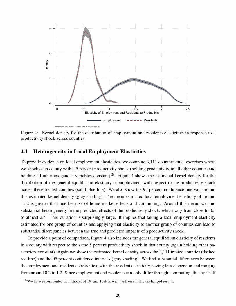
Figure 4: Kernel density for the distribution of employment and residents elasticities in response to aproductivity shock across counties
4.1 Heterogeneity in Local Employment Elasticities
To provide evidence on local employment elasticities, we compute 3,111 counterfactual exercises wherewe shock each county with a 5 percent productivity shock (holding productivity in all other counties andholding all other exogenous variables constant).26 Figure 4 shows the estimated kernel density for thedistribution of the general equilibrium elasticity of employment with respect to the productivity shockacross these treated counties (solid blue line). We also show the 95 percent confidence intervals aroundthis estimated kernel density (gray shading). The mean estimated local employment elasticity of around1.52 is greater than one because of home market effects and commuting. Around this mean, we findsubstantial heterogeneity in the predicted effects of the productivity shock, which vary from close to 0.5to almost 2.5. This variation is surprisingly large. It implies that taking a local employment elasticityestimated for one group of counties and applying that elasticity to another group of counties can lead tosubstantial discrepancies between the true and predicted impacts of a productivity shock.
To provide a point of comparison, Figure 4 also includes the general equilibrium elasticity of residentsin a county with respect to the same 5 percent productivity shock in that county (again holding other pa-rameters constant). Again we show the estimated kernel density across the 3,111 treated counties (dashedred line) and the 95 percent confidence intervals (gray shading). We find substantial differences betweenthe employment and residents elasticities, with the residents elasticity having less dispersion and rangingfrom around 0.2 to 1.2. Since employment and residents can only differ through commuting, this by itself
26We have experimented with shocks of 1% and 10% as well, with essentially unchanged results.
20

suggests that the heterogeneity in the local employment elasticity is largely driven by commuting linksbetween counties. In Section C.8 of the web appendix, we provide further evidence that this is indeed thecase by simulating productivity shocks in a counterfactual world without commuting between counties.Even in such a counterfactual world, we expect local employment elasticities to be heterogeneous, becausecounties differ substantially in terms of their initial shares of US employment. However, we find substan-tially less heterogeneity in local employment elasticities in this counterfactual world than in the actualworld with commuting. In fact, the resulting distribution of employment (and residential) elasticities issimilar to the one for residential elasticities in Figure 4.
In Subsection C.6 of the web appendix, we show that this heterogeneity in local employment elastic-ities remains if we shock counties with patterns of spatially correlated shocks reproducing the industrialcomposition of the U.S. economy. In Subsection C.10 of the web appendix, we find a similar pattern ofresults if we replicate our entire quantitative analysis for CZs rather than counties. Both sets of resultsare consistent with the fact that heterogeneous local employment elasticities are a generic prediction of agravity equation for commuting (as shown in Subsection B.8 of the web appendix). Although CZ bound-aries are drawn to minimize commuting, they inevitably cannot perfectly capture the rich geography ofcommuting flows implied by the gravity equation.
4.2 Explaining the Heterogeneity in Local Employment Elasticities
We now use the model to provide intuition on the determinants of the general equilibrium local employ-ment elasticities, dLi
dAi
AiLi
. We also use the structure of the model to determine a set of variables that canbe used empirically to account for the estimated heterogeneity in the distribution of local employmentelasticities. To do so, we compute partial equilibrium elasticities of own wages and own employmentwith respect to the productivity shock. These partial equilibrium elasticities capture the direct effect of aproductivity shock on wages, employment and residents in the treated location, holding constant all otherendogenous variables at their values in the initial equilibrium.27 Hence, although potentially useful to pro-vide intuition, or as empirical controls, they do not account for all the rich set of interactions in the modelcaptured by the general equilibrium elasticities presented in Figure 4.
If we hold constant all variables except for wi, Li, and Ri in the treated county i, the partial elasticityof employment with respect to the productivity shock is the product of the partial elasticity of employmentwith respect to wages and the partial elasticity of wages with respect to the productivity shock28
∂Li∂Ai
AiLi
=∂Li∂wi
wiLi· ∂wi∂Ai
Aiwi. (23)
From the equality between income and expenditure (8), the partial elasticity of wages with respect to the
27See Section B.7 in the web appendix for the derivation of these partial equilibrium elasticities.28Note that we use the partial derivative symbol, ∂Li
∂Ai
Ai
Li, to denote the partial equilibrium elasticity when we allow wi, Li
,and Ri to change but keep other variables in all other counties fixed.
21
productivity shock is given by
∂wi∂Ai
Aiwi
=(σ − 1)
∑n∈N (1− πni) ξni[
1 + (σ − 1)∑
n∈N (1− πni) ξni]
+[1−
∑n∈N (1− πni) ξni
]∂Li∂wi
wiLi− ξii ∂Ri∂wi
wiRi
. (24)
where ξni = πniαvnRn/wiLi is the share of location i’s revenue from market n.The intuition for the response of wages to the productivity shock can be seen most clearly for the case
when ∂Li∂wi
wiLi≈ 0 and ∂Ri
∂wi
wiRi≈ 0. From the terms in (σ − 1)
∑n∈N (1− πni) ξni, the elasticity of wages
with respect to productivity is high when location i accounts for a small share of expenditure (small πni) inmarkets n that account for a large share of its revenue (high ξni). In these circumstances, the productivityshock reduces the prices of location i’s goods and results in only a small reduction in the goods priceindices (small πni) in its main markets (high ξni).29 Therefore the productivity shock leads to a largeincrease in the demand for location i’s goods and hence in its wages. Thus
∑n∈N (1− πni) ξni provides a
measure of location i’s linkages to other locations in goods markets.From the commuter market clearing condition (14), the partial elasticity of employment with respect
to wages is∂Li∂wi
wiLi
= ε∑n∈N
(1− λni|n
)ϑni+ϑii
(∂Ri
∂wi
wiRi
), (25)
where ϑni = λni|nRn/Li is the share of commuters from residence n in workplace i’s employment.The intuition for the response of employment to wages can be seen most clearly for the case when
∂Ri∂wi
wiRi≈ 0. From the term in ε
∑n∈N
(1− λni|n
)ϑni, the elasticity of employment with respect to wages
is high when workplace i employs a small share of commuters (small λni|n) from residences n that supplya large fraction of its employment (high ϑni). In these circumstances, location i’s wage increase makes ita more attractive workplace and results in only a small increase in commuter market access (small λni|n)in its main sources of commuters (high ϑni).30 Therefore the increase in wages leads to a large increase incommuters to workplace i and hence in its employment. Thus
∑n∈N
(1− λni|n
)ϑni provides a measure
of workplace i’s linkages to other locations through commuting. In Subsection B.8 of the web appendix,we show that this partial elasticity takes the same form in the class of theoretical models consistent with agravity equation for commuting flows.
Using (12), the partial elasticity of residents with respect to wages is
∂Ri
∂wi
wiRi
= ε
(λiiλRi− λLi
), (26)
which also has an intuitive interpretation. A higher wage in location imakes it a more attractive workplaceand increases its employment. Whether this increase in location i’s employment leads to an increase in its
29These price indices summarize the price of competing varieties in each market. Note that the elasticity of the price index(9) in location n with respect to wages in location i is (∂Pn/∂wi) (wi/Pn) = πni.
30Commuter market access appears in the numerator of the residential choice probabilities (λRn in (12)) and summarizesaccess to employment opportunities: Wn =
[∑s∈N Bns (ws/κns)
ε]1/ε. Note that the elasticity of commuter market access inlocation n with respect to wages in location i is (∂Wn/∂wi) (wi/Wn) = λni|n.
22
share of residents depends on the fraction of residents who work locally (λii/λRi) relative to location i’soverall share of employment (λLi). Thus (λii/λRi − λLi) provides a measure of location i’s linkages toother locations through migration.
Combining the three elasticities in equations (24), (25), and (26), we obtain closed-form solutions forthe partial equilibrium elasticities of wages, employment and residents to a productivity shock. These par-tial equilibrium elasticities depend solely on the observed values of variables in the initial equilibrium: res-idential employment shares (λRi), conditional commuting probabilities (λni|n), employment shares (ϑni),trade shares (πni) and revenue shares (ξni).
When we undertake our counterfactuals, we solve for the full general equilibrium effect of the pro-ductivity shock to each county. But these partial equilibrium elasticities in terms of observed variableshave substantial explanatory power in predicting the impact of the productivity shock across locations, asnow shown in Table 2. In Column (1) we regress our general equilibrium elasticities on a constant, whichcaptures the mean employment elasticity across the 3,111 treated counties. In Columns (2) through (4) weattempt to explain the heterogeneity in local employment elasticities using standard county controls. InColumn (2) we include log county employment as a control for the size of economic activity in a county.In Column (3) we also include log county wages and log county land area. In Column (4) we also includethe average wage and total employment in neighboring counties. Although these controls are all typicallystatistically significant, we find that they are not particularly successful in explaining the variation in em-ployment elasticities. Adding a constant and all these controls yields an R-squared of only about 0.5 inColumn (4). Clearly, there is substantial variation not captured by these controls.
In the remaining columns of the table we attempt to explain the heterogeneity in local employmentelasticities using the partial equilibrium elasticities derived above. In Column (5) we first use the intuition(obtained by comparing the distributions in Figure 4) that commuting is important. As a summary statisticof the lack of commuting links of a county we use λii|i, namely, the share of workers that work in i
conditional on living in i. The weaker the commuting links of a county, the higher λii|i, which reducesthe local employment elasticity of that county. This is exactly what we find in Column (5). Furthermore,this variable alone yields an R-squared of 0.89, nearly double the R-squared in the regression where weinclude all the standard controls.31 Therefore, although the model incorporates several forms of spatiallinkages (including trade and migration), we find that the heterogeneity in local employment elasticities ismainly explained by commuting linkages, which is consistent with our gravity equation estimates, wherecommuting is substantially more local (higher distance coefficient) than goods trade.32
The partial equilibrium local elasticities computed above allow us to do better than just adding asummary measure of commuting links as the explanatory variable. In Column (6) we relate the vari-
31To provide further evidence on the magnitude of these effects, Table C.3 in Section C.4 of the web appendix reports thesame regressions as in Table 2 but using standardized coefficients. We find that a one standard deviation change in the owncommuting share (λii|i) leads to around a one standard deviation change in the local employment elasticity.
32In Subsection B.8 of the web appendix, we report kernel density estimates for the distribution of the partial equilibriummeasure of commuting linkages
∑n∈N
(1− λni|n
)ϑni that is a generic prediction of any commuting gravity equation. We
show a similar distribution of heterogeneous local employment elasticities to that in Figure 4 above, again confirming that thisheterogeneity is driven by commuting linkages.
23

ation in local employment elasticities to the measure of commuting linkages suggested by the model,∑n∈N
(1− λni|n
)ϑni. We also add the measures of migration and trade linkages suggested by the model,
(λii/λRi − λLi) and ∂wi∂Ai
Aiwi
. Including these partial equilibrium measures of linkages further increases theR-squared to around 93 percent of the variation in the general equilibrium elasticity. Counties that accountfor a small share of commuters (small λni|n) from their main suppliers of commuters (high ϑni) have higheremployment elasticities. In Column (7), we use the product of ∂wi
∂Ai
Aiwi
and the first two terms rather thaneach term separately. This restriction yields similar results and confirms the importance of commutinglinkages and, to a lesser extent, the interaction between migration and goods linkages. Finally, in the lasttwo columns we combine these partial equilibrium elasticities with the standard controls we used in thefirst four columns. Clearly, although all variables are significant, these standard controls add little once wecontrol for the partial equilibrium elasticities.
In sum, Table 2 shows that the heterogeneity in partial equilibrium elasticities is not well explained bystandard county controls. In contrast, adding a summary statistic of commuting, or the partial equilibriumelasticities we propose above, can go a long way in explaining this heterogeneity.
4.3 Positive Developed Land Supply Elasticities
In the baseline version of the model, we interpret the non-traded amenity as simply land, which is inperfectly inelastic supply. In this section, we develop an extension of the model, in which we interpret thenon-traded amenity as “developed” land and allow for a positive developed land supply elasticity that candiffer across locations.
We continue to assume the same specification of preferences, production and commuting decisions asin Section 2 above. We introduce a positive developed land supply elasticity by following Saiz (2010) inassuming that the supply of land (Hn) for each residence n depends on the endogenous price of land (Qn)as well as on the exogenous characteristics of locations (Hn):
Hn = HnQηnn , (27)
where ηn ≥ 0 is the developed land supply elasticity, which we allow to vary across locations; ηn = 0
is our baseline specification of a perfectly inelastic land supply; and ηn → ∞ is the special case of aperfectly elastic land supply.
Introducing a positive and heterogeneous developed land supply elasticity only affects one of the con-ditions for general equilibrium in the model, namely the land market clearing condition. Using the supplyfunction for land (27) in the land market clearing condition (5), we obtain the following generalization ofour earlier expression for the equilibrium price of land (Qn):
Qn =
((1− α)
vnRn
Hn
) 11+ηn
, (28)
where our baseline specification corresponds to the special case in which η = 0. Therefore, when under-
24
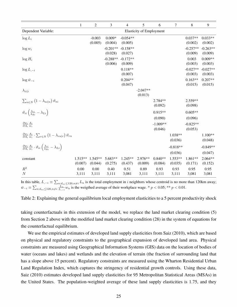
1 2 3 4 5 6 7 8 9
Dependent Variable: Elasticity of Employment
logLi -0.003 0.009* -0.054** 0.037** 0.033**(0.005) (0.004) (0.005) (0.002) (0.002)
logwi -0.201** -0.158** -0.257** -0.263**(0.028) (0.027) (0.009) (0.009)
logHi -0.288** -0.172** 0.003 0.009**(0.006) (0.009) (0.003) (0.003)
logL,−i 0.118** -0.027** -0.027**(0.007) (0.003) (0.003)
log w−i 0.204** 0.163** 0.207**(0.047) (0.015) (0.015)
λii|i -2.047**(0.013)∑
n∈N(1− λni|n
)ϑni 2.784** 2.559**
(0.092) (0.098)
ϑii
(λii
λRi− λLi
)0.915** 0.605**(0.090) (0.096)
∂wi
∂Ai
Ai
wi-1.009** -0.825**(0.046) (0.053)
∂wi
∂Ai
Ai
wi·∑r∈N
(1− λrn|r
)ϑrn 1.038** 1.100**
(0.036) (0.048)∂wi
∂Ai
Ai
wi· ϑii
(λii
λRi− λLi
)-0.818** -0.849**(0.036) (0.047)
constant 1.515** 1.545** 5.683** 1.245** 2.976** 0.840** 1.553** 1.861** 2.064**(0.007) (0.044) (0.275) (0.437) (0.009) (0.084) (0.035) (0.171) (0.152)
R2 0.00 0.00 0.40 0.51 0.89 0.93 0.93 0.95 0.95N 3,111 3,111 3,111 3,081 3,111 3,111 3,111 3,081 3,081
In this table, L,−i ≡∑n:dni≤120,n6=i Ln is the total employment in i neighbors whose centroid is no more than 120km away;
w−i ≡∑n:dni≤120,n6=i
Ln
L,−iwn is the weigthed average of their workplace wage. * p < 0.05; ** p < 0.01.
Table 2: Explaining the general equilibrium local employment elasticities to a 5 percent productivity shock
taking counterfactuals in this extension of the model, we replace the land market clearing condition (5)from Section 2 above with the modified land market clearing condition (28) in the system of equations forthe counterfactual equilibrium.
We use the empirical estimates of developed land supply elasticities from Saiz (2010), which are basedon physical and regulatory constraints to the geographical expansion of developed land area. Physicalconstraints are measured using Geographical Information Systems (GIS) data on the location of bodies ofwater (oceans and lakes) and wetlands and the elevation of terrain (the fraction of surrounding land thathas a slope above 15 percent). Regulatory constraints are measured using the Wharton Residential UrbanLand Regulation Index, which captures the stringency of residential growth controls. Using these data,Saiz (2010) estimates developed land supply elasticities for 95 Metropolitan Statistical Areas (MSAs) inthe United States. The population-weighted average of these land supply elasticities is 1.75, and they
25
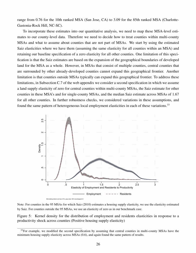
range from 0.76 for the 10th ranked MSA (San Jose, CA) to 3.09 for the 85th ranked MSA (Charlotte-Gastonia-Rock Hill, NC-SC).
To incorporate these estimates into our quantitative analysis, we need to map these MSA-level esti-mates to our county-level data. Therefore we need to decide how to treat counties within multi-countyMSAs and what to assume about counties that are not part of MSAs. We start by using the estimatedSaiz elasticities where we have them (assuming the same elasticity for all counties within an MSA) andretaining our baseline specification of a zero elasticity for all other counties. One limitation of this speci-fication is that the Saiz estimates are based on the expansion of the geographical boundaries of developedland for the MSA as a whole. However, in MSAs that consist of multiple counties, central counties thatare surrounded by other already-developed counties cannot expand this geographical frontier. Anotherlimitation is that counties outside MSAs typically can expand this geographical frontier. To address theselimitations, in Subsection C.7 of the web appendix we consider a second specification in which we assumea land supply elasticity of zero for central counties within multi-county MSAs, the Saiz estimate for othercounties in these MSA’s and for single-county MSAs, and the median Saiz estimate across MSAs of 1.67for all other counties. In further robustness checks, we considered variations in these assumptions, andfound the same pattern of heterogeneous local employment elasticities in each of these variations.33
0.5
11.
52
2.5
Den
sity
0 .5 1 1.5 2 2.5 3Elasticity of Employment and Residents to Productivity
Employment Residents
Eliminating bottom and top 0.5%; gray area: 95% boostrapped CI
Note: For counties in the 95 MSAs for which Saiz (2010) estimates a housing supply elasticity, we use the elasticity estimatedby Saiz. For counties outside the 95 MSAs, we use an elasticity of zero as in our benchmark case.
Figure 5: Kernel density for the distribution of employment and residents elasticities in response to aproductivity shock across counties (Positive housing supply elasticity)
33For example, we modified the second specification by assuming that central counties in multi-county MSAs have theminimum housing supply elasticity across MSAs (0.6), and again found the same pattern of results.
26

For each of these two specifications, we replicate our 3,111 counterfactual exercises where we shockeach county with a 5 percent productivity shock (holding productivity in all other counties and holding allother exogenous variables constant). Figure 5 displays the results, and is analogous to Figure 4 in the paper.The figure shows the estimated kernel density for the distribution of the general equilibrium elasticity ofboth employment (blue solid line) and residents (red dashed line) with respect to the productivity shockacross the treated counties. We also show the 95 percent confidence intervals around these estimatedkernel densities (gray shading). Consistent with the results for our baseline specification, we continue tofind substantial heterogeneity in local employment elasticities, confirming the robustness of our findingsto allowing for a variable developed land supply elasticity. Relative to our baseline specification, both theemployment and resident elasticities are somewhat larger in magnitude, as the elastic land supply dampensthe congestion effect from increased residents, and allows both employment and residents to increasemore than with a perfectly inelastic land supply. Compared with our baseline specification, we find moreheterogeneity in the resident elasticity. This pattern of results is also intuitive. Our baseline specificationfocuses on one source of heterogeneity (commuting), which mainly affects local employment elasticities.In this robustness test, we introduce a second source of heterogeneity (through variable developed landsupply elasticities), which mainly affects local resident elasticities (via residential land use). Thereforethe main consequence of adding this second source of heterogeneity is to generate greater dispersionin residential elasticities. Nevertheless, the dispersion in employment elasticities remains of around thesame magnitude as in our baseline specification. Furthermore, we continue to find substantial differencesbetween the elasticities for residents and employment, where the only way that these two elasticities candiffer from one another is through commuting.
4.4 Measuring the Incidence of Local Labor Demand Shocks
A large empirical literature is concerned with estimating the elasticity of local employment with respectto local labor demand shocks. The central specification in this empirical literature is a “differences-in-differences” specification across locations i and time t given by
∆ lnYit = a0 + a1Iit + a2Xit + uit, (29)
where Yit is the outcome of interest (e.g. employment by workplace); Iit is a measure of the local demandshock (treatment); Xit are controls; and uit is a stochastic error. The coefficient on the treatment a1
corresponds to the log change in the outcome of interest with respect to the local labor demand shock.This specification has a differences-in-differences interpretation, because the first difference is over time(before and after the shock), and the second difference is between treated and control counties.
We now compare the general equilibrium elasticities of employment with respect to the productivityshock in the model to the results of this type of reduced-form “differences-in-differences” estimates of thelocal average treatment effects of the productivity shock. In particular, we construct a regression sampleincluding both treated and untreated counties from our 3,111 counterfactuals in which we shock each
27

county in turn with a 5 percent productivity shock (3, 1112 = 9, 678, 321 observations). We use these datato estimate a “differences-in-differences” specification of a similar form to (29):
∆ lnYit = a0 + a1Iit + a2Xit + a3 (Iit ×Xit) + uit,
where i denotes the 3,111 counties and t indexes the 3,111 counterfactuals; ∆ lnYit is the change in logemployment between the counterfactual and actual equilibria; Iit is a (0,1) indicator for whether a countyis treated with a productivity shock; and Xit are controls. We again consider two sets of controls (Xit):the model-suggested measures of linkages in goods and factor markets and more standard econometriccontrols (log employment, log wages and land area). We include both the main effects of these controls(captured by a2) and their interactions with the treatment indicator to capture heterogeneity in the treatmenteffects (captured by a3).
A key difference between this regression specification and the above results for the general equilibriumelasticities for the treated counties is that this regression specification differences relative to the untreatedcounties. The empirical literature has argued for the need to difference relative to untreated counties giventhe likely presence of other shocks or events, beyond the treatment, that can affect the treated countiessimultaneously and can confound the true treatment effect. Of course, our synthetic dataset was generatedwithout including any of these alternative shocks and so differencing is not needed in order to calculatethe correct treatment effects.
In a specification without the controls (a2 = a3 = 0), the average effect of the productivity shock onthe untreated counties is captured in the regression constant (a0), and the local average treatment effect (a1)corresponds to the difference in means between the treated and untreated counties. We compare estimatingthis regression specification including (i) a random untreated county in the control group, (ii) only thenearest untreated county in the control group, (iii) only neighboring counties within 120 kilometers of thetreated county in the control group, (iv) only non-neighboring counties located from 120-240 kilometersfrom the treated county, and (v) all untreated counties in the control group.
We compare the predicted treatment effect from the “differences-in-differences” specification to thegeneral equilibrium employment elasticity in the model by computing the following deviation term for thetreated county:
βi =a1 + a3Xit
0.05− dLidAi
AiLi, (30)
which corresponds to the difference between the predicted treatment effect, scaled by the size of theproductivity shock, and the general equilibrium employment elasticity in the model. In Figure 6 we showkernel densities of the distribution of this deviation term across the 3,111 counterfactuals for productivityshocks to each county. We show the deviation term using model-suggested controls (solid lines) andreduced-form controls (dashed lines). We display these results for each of the alternative control groupsconsidered above ((i) to (v)).
28
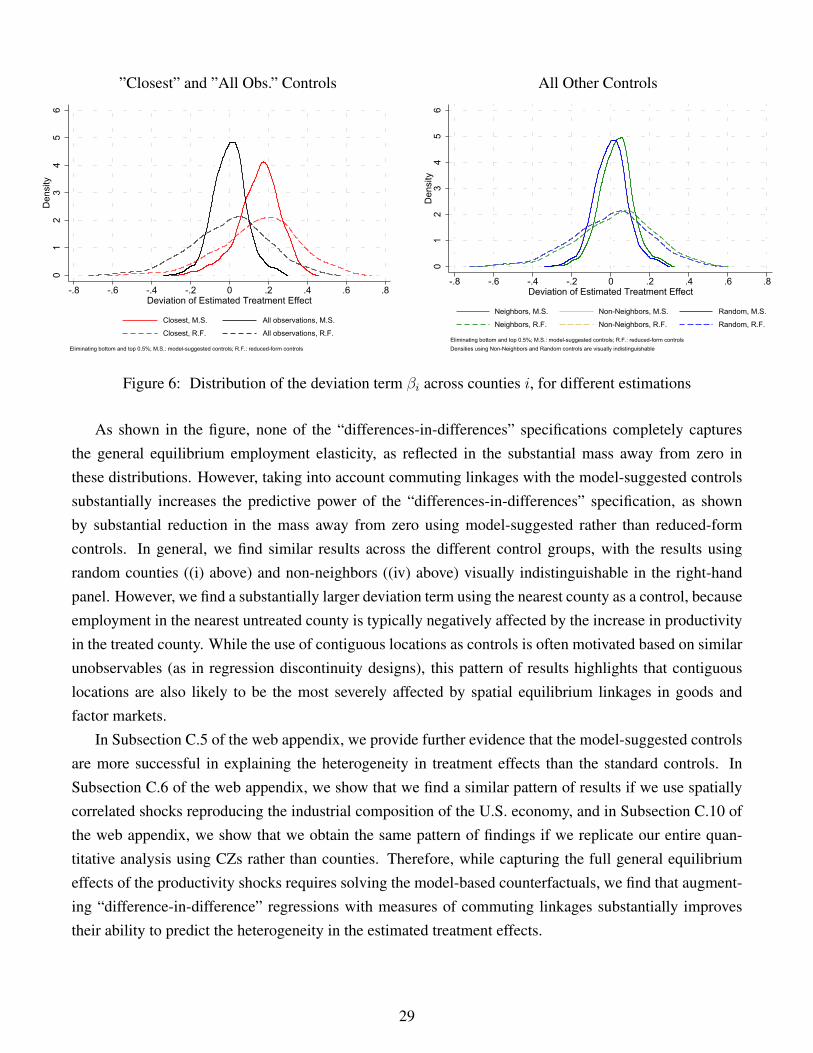
”Closest” and ”All Obs.” Controls All Other Controls
01
23
45
6D
ensi
ty
-.8 -.6 -.4 -.2 0 .2 .4 .6 .8Deviation of Estimated Treatment Effect
Closest, M.S. All observations, M.S.
Closest, R.F. All observations, R.F.
Eliminating bottom and top 0.5%; M.S.: model-suggested controls; R.F.: reduced-form controls
01
23
45
6D
ensi
ty
-.8 -.6 -.4 -.2 0 .2 .4 .6 .8Deviation of Estimated Treatment Effect
Neighbors, M.S. Non-Neighbors, M.S. Random, M.S.
Neighbors, R.F. Non-Neighbors, R.F. Random, R.F.
Eliminating bottom and top 0.5%; M.S.: model-suggested controls; R.F.: reduced-form controlsDensities using Non-Neighbors and Random controls are visually indistinguishable
0123456Density-.8-.6-.4-.20.2.4.6.8Deviation of Estimated Treatment EffectClosest, M.S.All observations, M.S.Closest, R.F.All observations, R.F.Eliminating bottom and top 0.5%; M.S.: model-suggested controls; R.F.: reduced-form controls
Figure 6: Distribution of the deviation term βi across counties i, for different estimations
As shown in the figure, none of the “differences-in-differences” specifications completely capturesthe general equilibrium employment elasticity, as reflected in the substantial mass away from zero inthese distributions. However, taking into account commuting linkages with the model-suggested controlssubstantially increases the predictive power of the “differences-in-differences” specification, as shownby substantial reduction in the mass away from zero using model-suggested rather than reduced-formcontrols. In general, we find similar results across the different control groups, with the results usingrandom counties ((i) above) and non-neighbors ((iv) above) visually indistinguishable in the right-handpanel. However, we find a substantially larger deviation term using the nearest county as a control, becauseemployment in the nearest untreated county is typically negatively affected by the increase in productivityin the treated county. While the use of contiguous locations as controls is often motivated based on similarunobservables (as in regression discontinuity designs), this pattern of results highlights that contiguouslocations are also likely to be the most severely affected by spatial equilibrium linkages in goods andfactor markets.
In Subsection C.5 of the web appendix, we provide further evidence that the model-suggested controlsare more successful in explaining the heterogeneity in treatment effects than the standard controls. InSubsection C.6 of the web appendix, we show that we find a similar pattern of results if we use spatiallycorrelated shocks reproducing the industrial composition of the U.S. economy, and in Subsection C.10 ofthe web appendix, we show that we obtain the same pattern of findings if we replicate our entire quan-titative analysis using CZs rather than counties. Therefore, while capturing the full general equilibriumeffects of the productivity shocks requires solving the model-based counterfactuals, we find that augment-ing “difference-in-difference” regressions with measures of commuting linkages substantially improvestheir ability to predict the heterogeneity in the estimated treatment effects.
29

4.5 Million Dollar Plants Natural Experiment
Having established the heterogeneity of local employment elasticities in our quantitative model, due todifferences in commuting linkages across counties, we now use evidence from a natural experiment toprovide independent verification of this prediction in the data. In particular, we use the natural experimentof million dollar plants (MDP) from GHM (2010), one of the most influential papers in the local labor mar-kets literature. The identification strategy compares employment in “winning” and “runner-up” countiesbefore and after the opening of a MDP. As the runner-up counties are those that survived a long selectionprocess, but narrowly lost the competition to winning counties, one would expect the two groups to havesimilar initial characteristics. Consistent with this, GHM show that winning and runner-up counties aresimilar along a range of observables before a MDP opening. In contrast, GHM show that the two groupsexhibit sharply different trajectories following a MDP opening: winning counties experience larger plant-level increases in total factor productivity (TFP), and have larger county-level increases in the number ofmanufacturing plants and total manufacturing employment and output.
For our empirical analysis, we start with a list of 82 MDP announcements (“cases”) containing winnerand runner-up counties from the corporate real estate journal Site Selection, as reported in Greenstone andMoretti (2004). Only a subset of 47 of these MDP announcements could be located in confidential censusdata by GHM (2010), in part because not all of the announced plants were necessarily ultimately opened.To be conservative (and because the census data are confidential), we use the full list of 82 announcements,where the fact that some of these plants may not have actually opened (or may have opened some time afterthe announcement date) will make it harder for us to find discernible effects. We begin by estimating theaverage treatment effect of a MDP announcement. Consistent with the reduced-form specification fromthe previous subsection, we estimate a “differences-in-differences” regression, where the first difference isbefore and after the announcement, and the second difference is between winning and runner-up counties.For each year τ > 0 after the announcement of a MDP, we difference log county employment relative toits value in the year of the announcement (τ = 0) and estimate a specification given by
∆ lnYikτ = ατ Iikτ + µkτ + uikτ (31)
where i again indexes counties and k denotes cases (instances of winner and runner-up counties); weestimate this regression separately for each year τ > 0; ∆ lnYikτ is the change in log employment betweenthe announcement and year τ ; the first differencing over time has eliminated any county fixed effect in thelevel of log employment; Iikτ is a treatment indicator that equals one if a county i for case k has anannounced MDP in year τ and zero otherwise; µkτ is a case fixed effect that captures average employmentgrowth up to year τ for both the winner and runner-up counties in case k; ατ is the key coefficient ofinterest and corresponds to the average treatment effect of a MDP announcement.
We next examine the extent to which the treatment effect of a MDP announcement is heterogeneousacross counties depending on their commuting linkages, as predicted by our quantitative model. Motivatedby the results of our counterfactuals in the previous section, we measure these commuting linkages using
30

each county’s own commuting share. We augment the “differences-in-differences” regression in (31)with both the main effect of the own commuting share (λii|i) and the interaction term between the MDPannouncement and the own commuting share (λii|i × Iikτ ). So we estimate
∆ lnYikτ = ατ Iikτ + βτλii|i + γτ(λii|i × Iikτ
)+ µkτ + uikτ , (32)
where the coefficient βτ on the main effect allows for the possibility that counties open versus closed tocommuting could differ in employment growth for other reasons besides the MDP announcement; the keycoefficient of interest is γτ on the interaction term, which captures heterogeneity in the response of localemployment to the MDP announcement. Based on our quantitative model, we expect γτ to be negative andstatistically statistically significant, such that counties more closed to commuting (higher own commutingshares λii|i) have smaller local employment responses.
In Table 3, we report the estimation results. To provide a point of comparison, Panel A estimates equa-tion (31) including only the case fixed effects (without the treatment indicator). Across periods ranging upto five years after the MDP announcement, we find that the case fixed effects alone explain around 18 to29 percent of the variance in county employment growth. In Panel B, we estimate the average treatmenteffect of the MDP announcement using our baseline specification (31) (including the treatment indicator).We find strong confirmation of the empirical results in GHM (2010), with a positive and statistically sig-nificant average treatment effect. The magnitude of this treatment effect is substantial, ranging from 2.6percent to more than 6 percent as we move from one to five years after the announcement. We also findthat the MDP announcement has substantial explanatory power for county employment growth, with theregression R-squared rising to a range of 27 to 29 percent.
In Panel C, we estimate heterogeneous treatment effects using our augmented specification (32) (in-cluding the own commuting share terms). Confirming our model’s predictions, the estimated coefficienton the interaction term (γτ ) is negative and statistically significant, implying that the MDP announcementhas smaller employment effects in counties more closed to commuting. The implied magnitude of thisheterogeneity is large compared to the average treatment effect of 2 to 6 percent from Panel B. For acounty with an own commuting share at the 75th percentile the predicted employment effect is between23.6 and 26.6 percent (depending on the number of years after the treatment) smaller than for a countywith a commuting share at the 25th percentile. In fact, in our quantitative model, the same exercise usingsimulated data yields a slightly smaller reduction in the predicted employment effect (18.2 percent). Ifwe compare the 90th and 10th percentile of own commuting shares the difference in employment effectsranges between 49% and 43% (again depending on the number of years after treatment). In our quanti-tative model, the same difference is 31.7%. We conclude that the impact of commuting linkages on theemployment response to the MDP is statistically significant and large in economic terms. The reductionsin the employment effect of the treatment that result from higher own commuting shares are of the samemagnitude, but somewhat larger, than the ones predicted by our quantitative model. So, if anything, ourmodel seems to underplay the importance of commuting compared to the data.
31

Panel A : Case Fixed Effects Onlyτ years after Adj R2
1 0.212 0.293 0.254 0.225 0.18
Panel B : Average Treatment Effect and Case Fixed Effectsτ years after Adj R2 Coefficient Std. Error
1 0.31 0.026∗∗∗ 0.0062 0.39 0.038∗∗∗ 0.0083 0.36 0.050∗∗∗ 0.0104 0.31 0.053∗∗∗ 0.0135 0.27 0.062∗∗∗ 0.015
Panel C : Heterogeneous Treatment Effects and Case Fixed EffectsTreatment Openness Interaction
τ years after Adj R2 Coefficient Std. Error Coefficient Std Error Coefficient Std Error1 0.40 0.117∗∗ 0.028 -0.027 0.026 -0.124∗∗∗ 0.0362 0.50 0.133∗∗ 0.037 -0.084∗∗∗ 0.035 -0.133∗∗∗ 0.0483 0.46 0.149∗∗ 0.048 -0.130∗∗∗ 0.045 -0.140∗∗∗ 0.0624 0.41 0.159∗ 0.059 -0.167∗∗∗ 0.056 -0.151∗∗ 0.0775 0.39 0.213∗ 0.071 -0.191∗∗∗ 0.067 -0.213∗∗ 0.092
This table reports estimates of versions of equations (31) and (32). Case fixed effects are never reported. Panel A estimatesequation (31) including only the case fixed effects µkτ (i.e. without the treatment indicator Iikτ ). Panel B estimates the averagetreatment effect of the MDP announcement using specification (31). Panel C estimates heterogeneous treatment effects usingspecification (32). In Panel C, “Treatment” refers to the coefficient ατ , “Openness” refers to the coefficient βτ , and “Interaction”refers to the coefficient γτ as in equation (32). * p < 0.1; ** p < 0.05; *** p < 0.01.
Table 3: Million Dollar Plants Natural Experiment
We also find a negative and statistically significant main effect (βτ ) of the own commuting share,consistent with counties that are more closed to commuting growing more slowly on average. ComparingPanels C and B, allowing for heterogeneous treatment effects leads to a substantial further increase inthe regression R-squared to 40-50 percent. Therefore the increase in explanatory power from allowingfor treatment heterogeneity depending on commuting links is around as large as that from allowing foraverage treatment effects (Panels A-B).
Finally, the results in Table 3 also indicate that the average treatment effects estimated by GHM (2010)depend on the average amount of commuting in the economy at the time of the treatment. An economywith larger average own commuting shares generates smaller average treatment effects than an economywith smaller own commuting shares. This elasticity is governed by γτ , which is highly significant andincreases in absolute magnitude (declines from −0.124 to −0.213) over the first five years after treatment.
Taking the results of this section together, using the natural experiment of million dollar plants (MDP)as an independent source of variation, we find strong confirmation of our model’s prediction of hetero-geneous local employment elasticities depending on commuting networks. Comparing counties that areotherwise similar, except for whether they were ultimately fortunate enough to attract a MDP, we find sub-stantially larger increases in employment in winner counties than in runner-up counties, and this increase
32
in employment is considerably greater for those winner counties that are more open to commuting.
5 Changes in Commuting Costs
In the previous sections, we have shown the importance of commuting for the effects of local labor demandshocks. We now show that it also matters in the aggregate for the spatial distribution of economic activityacross locations and welfare. Commuting enables workers to access high productivity locations withouthaving to pay the high cost of living in those locations. Increasing the cost of commuting restricts theopportunity set available to firms and workers and hence is expected to reduce welfare. Locations thatwere previously net exporters of commuters in the initial equilibrium become less attractive residences,while locations that were previously net importers of commuters in the initial equilibrium become lessattractive workplaces. As agents relocate in response to the restricted opportunity set, we also expect adecline in the specialization of counties as residential or business locations.
We begin by using the observed commuting data to back out implied values of the composite parametercapturing the ease of commuting (Bni ≡ Bniκ
−εni ). Following Head and Ries (2001) in the international
trade literature, we use the flows of commuters between locations n and i in both directions relative to theirown commuting flows. Using the commuting gravity equation (11), and taking the geometric mean ofthese relative flows in both directions, we obtain the following measure of the average ease of commutingbetween locations n and i relative to the ease of commuting to themselves:
Bni ≡(BniBnnBinBii
)1/2
=
(LniLnn
LinLii
)1/2
. (33)
We compute this measure for both 1990 and 2010. Between these two years, both miles of paved roads andvehicle kilometers travelled increased substantially.34 Consistent with this, we find a substantial increasein the relative ease of commuting from 4 percent ( ˆBni = 0.96) at the 25th percentile, to 12 percent( ˆBni = 0.88) at the median, and 21 percent ( ˆBni = 0.79) at the 75th percentile.
We use this distribution of implied changes in the relative ease of commuting to undertake counterfac-tuals for empirically-realistic changes in commuting costs. We assume a common reduction or increasein the costs of commuting for all counties equal to percentiles of this distribution (e.g. we assume thatall counties experience a reduction in commuting costs equal to the median value of ˆBni). Given thisassumption, we use the system of equations for general equilibrium in the model to solve for the newcounterfactual equilibrium after the reduction in commuting costs, as discussed in Section 2.6 above. Us-ing the commuting probability (11), expected utility (16), the price index (9) and land market clearing (5),the change in the common level of welfare across all locations from the shock to commuting costs can be
34Between 1990 and 2010, kilometers of paved public roads in the United States increased by over 20 percent (from 3.6 to4.4 million), and vehicle kilometers travelled increased by more than 38 percent (from 3,451,016 to 4,775,352 million). Forfurther discussion of this expansion in transport use, see for example Duranton and Turner (2011).
33
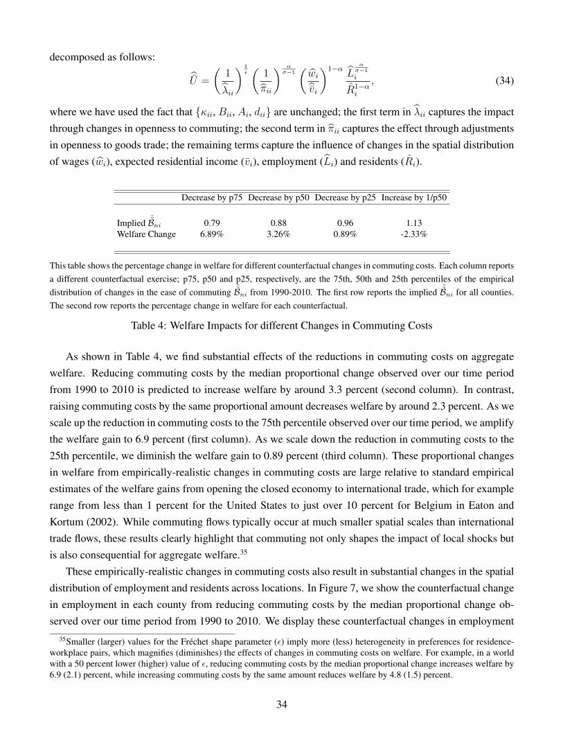
decomposed as follows: U =
(1
λii
) 1ε(
1
πii
) ασ−1(wivi)1−α
Lασ−1
i
R1−αi
, (34)
where we have used the fact that {κii, Bii, Ai, dii} are unchanged; the first term in λii captures the impactthrough changes in openness to commuting; the second term in πii captures the effect through adjustmentsin openness to goods trade; the remaining terms capture the influence of changes in the spatial distributionof wages (wi), expected residential income (vi), employment (Li) and residents (Ri).
Decrease by p75 Decrease by p50 Decrease by p25 Increase by 1/p50
Implied ˆBni 0.79 0.88 0.96 1.13Welfare Change 6.89% 3.26% 0.89% -2.33%
This table shows the percentage change in welfare for different counterfactual changes in commuting costs. Each column reportsa different counterfactual exercise; p75, p50 and p25, respectively, are the 75th, 50th and 25th percentiles of the empiricaldistribution of changes in the ease of commuting ˆBni from 1990-2010. The first row reports the implied ˆBni for all counties.The second row reports the percentage change in welfare for each counterfactual.
Table 4: Welfare Impacts for different Changes in Commuting Costs
As shown in Table 4, we find substantial effects of the reductions in commuting costs on aggregatewelfare. Reducing commuting costs by the median proportional change observed over our time periodfrom 1990 to 2010 is predicted to increase welfare by around 3.3 percent (second column). In contrast,raising commuting costs by the same proportional amount decreases welfare by around 2.3 percent. As wescale up the reduction in commuting costs to the 75th percentile observed over our time period, we amplifythe welfare gain to 6.9 percent (first column). As we scale down the reduction in commuting costs to the25th percentile, we diminish the welfare gain to 0.89 percent (third column). These proportional changesin welfare from empirically-realistic changes in commuting costs are large relative to standard empiricalestimates of the welfare gains from opening the closed economy to international trade, which for examplerange from less than 1 percent for the United States to just over 10 percent for Belgium in Eaton andKortum (2002). While commuting flows typically occur at much smaller spatial scales than internationaltrade flows, these results clearly highlight that commuting not only shapes the impact of local shocks butis also consequential for aggregate welfare.35
These empirically-realistic changes in commuting costs also result in substantial changes in the spatialdistribution of employment and residents across locations. In Figure 7, we show the counterfactual changein employment in each county from reducing commuting costs by the median proportional change ob-served over our time period from 1990 to 2010. We display these counterfactual changes in employment
35Smaller (larger) values for the Frechet shape parameter (ε) imply more (less) heterogeneity in preferences for residence-workplace pairs, which magnifies (diminishes) the effects of changes in commuting costs on welfare. For example, in a worldwith a 50 percent lower (higher) value of ε, reducing commuting costs by the median proportional change increases welfare by6.9 (2.1) percent, while increasing commuting costs by the same amount reduces welfare by 4.8 (1.5) percent.
34
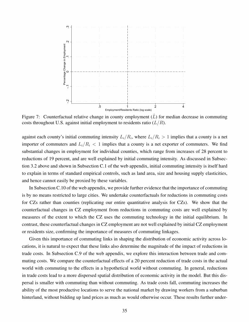
-.2-.1
0.1
.2.3
Per
cent
age
Cha
nge
in E
mpl
oym
ent
.5 1 2 4Employment/Residents Ratio (log scale)
Figure 7: Counterfactual relative change in county employment (L) for median decrease in commutingcosts throughout U.S. against initial employment to residents ratio (L/R).
against each county’s initial commuting intensity Li/Ri, where Li/Ri > 1 implies that a county is a netimporter of commuters and Li/Ri < 1 implies that a county is a net exporter of commuters. We findsubstantial changes in employment for individual counties, which range from increases of 28 percent toreductions of 19 percent, and are well explained by initial commuting intensity. As discussed in Subsec-tion 3.2 above and shown in Subsection C.1 of the web appendix, initial commuting intensity is itself hardto explain in terms of standard empirical controls, such as land area, size and housing supply elasticities,and hence cannot easily be proxied by these variables.
In Subsection C.10 of the web appendix, we provide further evidence that the importance of commutingis by no means restricted to large cities. We undertake counterfactuals for reductions in commuting costsfor CZs rather than counties (replicating our entire quantitative analysis for CZs). We show that thecounterfactual changes in CZ employment from reductions in commuting costs are well explained bymeasures of the extent to which the CZ uses the commuting technology in the initial equilibrium. Incontrast, these counterfactual changes in CZ employment are not well explained by initial CZ employmentor residents size, confirming the importance of measures of commuting linkages.
Given this importance of commuting links in shaping the distribution of economic activity across lo-cations, it is natural to expect that these links also determine the magnitude of the impact of reductions intrade costs. In Subsection C.9 of the web appendix, we explore this interaction between trade and com-muting costs. We compare the counterfactual effects of a 20 percent reduction of trade costs in the actualworld with commuting to the effects in a hypothetical world without commuting. In general, reductionsin trade costs lead to a more dispersed spatial distribution of economic activity in the model. But this dis-persal is smaller with commuting than without commuting. As trade costs fall, commuting increases theability of the most productive locations to serve the national market by drawing workers from a suburbanhinterland, without bidding up land prices as much as would otherwise occur. These results further under-
35
score the prominence of commuting linkages in shaping the equilibrium spatial distribution of economicactivity, and the necessity of incorporating them in models of economic geography.
6 Conclusions
The economic effects of local labor demand shocks have been the subject of an extensive empirical liter-ature on local labor markets, which has considered a wide range of such shocks, including industry com-position, international trade, macro and financial crises, and natural resource discoveries, among others.To understand the impact of these types of shocks, we develop a quantitative spatial general equilibriummodel that incorporates spatial linkages between locations in both goods markets (trade) and factor mar-kets (commuting and migration). Although we allow for a large number of locations and a rich geographyin both goods and factor markets, we provide analytical results for the existence and uniqueness of thegeneral equilibrium. We show how the model can be quantified using available data to match the observedgravity equation relationships for trade in goods and commuting, as well as the observed cross-sectiondistributions of employment, residents and wages. Thus, our framework provides a tractable platform forundertaking a range of counterfactuals for realistic changes in trade and commuting costs.
Whereas previous research has largely treated local labor markets as independent observations in cross-section regressions, we explicitly model the spatial linkages between these locations, which enables us toundertake our analysis at different levels of spatial aggregation. Through modeling these linkages, weovercome a trade-off faced in existing research, namely that choosing larger spatial units reduces un-modeled spatial linkages between locations, but also reduces the ability to make inferences about locallabor markets. We show that commuting flows are substantial and heterogeneous across both countiesand commuting zones (CZs) in the United States. Although the boundaries of CZs are chosen to mini-mize commuting, no choice of boundaries is able to fully capture the rich geography of commuting flowsimplied by the gravity equation.
Commuting allows workers to separate their workplace and residence, thereby introducing a quantita-tively relevant distinction between the effects of local labor demand shocks on employment and residents.We find substantial heterogeneity across both counties and CZs in the elasticity of local employment to aproductivity shock, which ranges from around 0.5 to 2.5. Therefore an average local employment elasticityestimated in one context can be quite misleading if applied in another context without controlling for thisheterogeneity. We show that this heterogeneity is hard to explain with standard empirical controls, such asarea and size, but is well explained by measures of linkages in commuting networks. We use our modelto highlight a simple summary statistic of the share of residents that work locally that can be included inreduced-form regressions to control for this heterogeneity.
We show that our finding of heterogeneous local employment elasticities is robust across a wide rangeof different specifications, including the introduction of differences in supply elasticities for developedland. These findings are consistent with such heterogeneity being a generic prediction of a commutinggravity equation, which is a strong empirical feature of the data. We also use the natural experiment of
36
million dollar plants (MDPs) to provide further independent empirical support for our model’s predictions.We compare counties that are otherwise similar, except for whether they were ultimately fortunate enoughto attract a MDP. We find substantially larger increases in employment in winner counties than in runner-upcounties, and this increase in employment is considerably greater for those winner counties more open tocommuting. Finally, as well as shaping the effects of local labor demand shocks, we show that commutingalso matters in the aggregate for the spatial distribution of economic activity and welfare. We use observedcommuting flows between pairs of counties over time to back out the empirical distribution of impliedreductions in commuting costs from 1990-2010. Reducing commuting costs for all counties by the medianof this empirical distribution, we find an increase in welfare of 3.3 percent, and employment changes acrosscounties that range from increases of 28 percent to reductions of 19 percent.
The quantitative model we propose is, we believe, ambitious and rich, yet its core insights are also rela-tively general. So we hope that our results are used to motivate the inclusion of measures of commuting infuture estimation of local employment elasticities. Their inclusion is simple, practical, and well groundedin theory.
References
[1] Ahlfeldt, Gabriel, Stephen Redding, Daniel Sturm and Nikolaus Wolf (2015) “The Economics ofDensity: Evidence from the Berlin Wall,” Econometrica, 83(6), 2127-2189.
[2] Allen, Treb, and Costas Arkolakis (2014) “Trade and the Topography of the Spatial Economy,” Quar-
terly Journal of Economics, 129(3), 1085-1140.
[3] Allen, Treb, Costas Arkolakis and Yuta Takahashi (2014) “Universal Gravity,” NBER Working Paper,20787.
[4] Allen, Treb, Costas Arkolakis and Xiangliang Li (2015) “Optimal City Structure,” Yale University,mimeograph.
[5] Alonso, William (1964) Location and Land Use, Cambridge MA: Harvard.
[6] Arkolakis, Costas, Arnaud Costinot and Andres Rodriguez-Clare (2012) “New Trade Models, SameOld Gains,” American Economic Review, 102(1), 94-130.
[7] Armington, Paul S. (1969) “A Theory of Demand for Products Distinguished by Place of Production,”IMF Staff Papers, 16(1), 159-178.
[8] Artuc, E., S. Chaudhuri, and J. McLaren (2010) “Trade Shocks and Labor Adjustment: A StructuralEmpirical Approach,” American Economic Review, 100(3), 1008-1045.
[9] Autor David, David Dorn and Gordon Hanson (2013) “The China Syndrome: Local Labor MarketEffects of Import Competition in the United States,” American Economic Review, 103(6), 2121-2168.
[10] Bartik, Timothy J. (1991) “Who Benefits from State and Local Economic Development Policies?”W.E. Upjohn Institute for Employment Research, Upjohn Press.
37

[11] Behrens, K., G. Mion, Y. Murata and J. Sudekum, 2014. ”Spatial frictions,” DICE Discussion Pa-pers 160, Heinrich-Heine-Universitat Dusseldorf, Dusseldorf Institute for Competition Economics(DICE).
[12] Blanchard, Olivier Jean, and Lawrence F. Katz (1992) “Regional Evolutions,” Brookings Papers on
Economic Activity, 23(1), 1-76.
[13] Bound, John and Holzer, Harry J (2000) “Demand Shifts, Population Adjustments, and Labor MarketOutcomes during the 1980s,” Journal of Labor Economics, 18(1), 20-54.
[14] Broda, Christian and David E. Weinstein (2006) “Globalization and the Gains from Variety,” Quar-
terly Journal of Economics, 121(2), 541-86.
[15] Busso, M., J. Gregory, and P. Kline (2013) “Assessing the Incidence and Efficiency of a ProminentPlace Based Policy,” American Economic Review, 103(2), 897-947.
[16] Caliendo, L. and F. Parro (2015) “Estimates of the Trade and Welfare Effects of NAFTA,” Review of
Economic Studies, 82(1), 1-44.
[17] Caliendo, L., F. Parro, E. Rossi-Hansberg, and P.-D. Sarte (2014) “The Impact of Regional andSectoral Productivity Changes on the U.S. Economy,” NBER Working Paper, 20168.
[18] Dekle, R., J. Eaton, and S. Kortum (2007) “Unbalanced Trade,” American Economic Review, 97(2),351-355.
[19] Desmet, Klaus and Esteban Rossi-Hansberg (2013) “Urban Accounting and Welfare,” American Eco-
nomic Review, 103:6, 2296-2327.
[20] Desmet, Klaus and Esteban Rossi-Hansberg (2014) “Spatial Development,” American Economic Re-
view, 104(4), 1211-1243.
[21] Diamond, Rebecca (2016) “The Determinants and Welfare Implications of US Workers? DivergingLocation Choices by Skill: 1980-2000,” American Economic Review, 106(3), 479-524.
[22] Dingel, Jonathan (2015) “The Determinants of Quality Specialization,” Chicago Booth School ofBusiness, mimeograph.
[23] Duranton, Gilles and Matthew A. Turner (2011) “The Fundamental Law of Road Congestion: Evi-dence from U.S. Cities,” American Economic Review, 101(6), 2616-2652.
[24] Duranton, Gilles, Peter Morrow and Matthew A. Turner (2014) “Roads and Trade: Evidence fromthe U.S.,” Review of Economic Studies, 81(2), 681-724.
[25] Eaton, Jonathan and Kortum, Samuel (2002) “Technology, Geography, and Trade,” Econometrica,70(5), 1741-1779.
[26] Feyrer, James, Erin T. Mansur and Bruce Sacerdote (2015) “Geographic dispersion of economicshocks: Evidence from the fracking revolution” NBER Working Paper, 21624.
[27] Fujita, Masahisa, Paul Krugman and Anthony J. Venables (1999) The Spatial Economy: Cities,
Regions and International Trade, Cambridge: MIT Press.
38

[28] Greenstone, M. and E. Moretti (2004) “Bidding for Industrial Plants: Does Winning a ‘Million DollarPlant’ Increase Welfare? ” NBER Working Paper, 9844.
[29] Greenstone, M., R. Hornbeck, and E. Moretti (2010) “Identifying Agglomeration Spillovers: Evi-dence from Winners and Losers of Large Plant Openings,” Journal of Political Economy, 118(3),536-598.
[30] Grogger, J., and G. Hanson (2011) “Income Maximization and the Selection and Sorting of Interna-tional Migrants,” Journal of Development Economics, 95(1), 42-57.
[31] Hanson, G. H. (1996) “Localization Economies, Vertical Organization, and Trade,” American Eco-
nomic Review, 86(5), 1266-1278.
[32] Hanson, Gordon H. (2005) “Market Potential, Increasing Returns, and Geographic Concentration,”Journal of International Economics, 67(1), 1-24.
[33] Head, Keith and John Ries (2001) “Increasing Returns versus National Product Differentiation,”American Economic Review, 91, 858-876.
[34] Helpman, Elhanan (1998) “The Size of Regions,” In Topics in Public Economics: Theoretical and
Applied Analysis, ed. David Pines, Efraim Sadka, and Itzhak Zilcha, Cambridge: Cambridge Univer-sity Press.
[35] Kennan, J., and J. R. Walker (2011) “The Effect of Expected Income on Individual Migration Deci-sions,” Econometrica, 79(1), 211-251.
[36] Krugman, Paul (1991) “Increasing Returns and Economic Geography,” Journal of Political Economy,99(3), 483-99.
[37] Krugman, Paul and Anthony J. Venables (1995) “Globalization and the Inequality of Nations,” Quar-
terly Journal of Economics, 110(4), 857-880.
[38] Lucas, Robert E. and Esteban Rossi-Hansberg (2002) “On the Internal Structure of Cities”, Econo-
metrica, 70(4), 1445-76.
[39] Manning, Alan and Barbara Petrongolo (2011) “How Local are Labour Markets? Evidence from aSpatial Search Model”, CEP Discussion Paper, No. 1101, London School of Economics.
[40] McFadden, D. (1974) “The Measurement of Urban Travel Demand,” Journal of Public Economics,3(4), 303-328.
[41] McFadden, Daniel and Kenneth Train (2000) “Mixed MNL Models of Discrete Response,” Journal
of Applied Econometrics, 15, 447-470.
[42] Melitz, Marc J. (2003) “The Impact of Trade on Intra-Industry Reallocations and Aggregate IndustryProductivity,” Econometrica, 71(6), 1695-1725.
[43] Mian, Atif and Amir Sufi (2014) “What Explains the 2007-2009 Drop in Employment?” Economet-
rica, 82(6), 2197-2223.
[44] Michaels, Guy (2011) “The Long Term Consequences of Resource-Based Specialisation,” Economic
Journal, 121(551), 31-57.
39

[45] Mills, Edwin S. (1967) “An Aggregative Model of Resource Allocation in a Metropolitan Centre,”American Economic Review, 57(2), 197-210.
[46] Monte, Ferdinando (2016) “The Local Incidence of Trade Shocks,” Georgetown University, mimeo-graph.
[47] Moretti, Enrico (2011) “Local Labor Markets,” in Handbook of Labor Economics, (ed.) D. Card, andO. Ashenfelter, Volume 4b, Amsterdam: Elsevier North Holland, 1238-1303.
[48] Moretti, Enrico and Patrick Klein (2011) “Local Economic Development, AgglomerationEconomies, and the Big Push: 100 Years of Evidence from the Tennessee Valley Authority,” Quar-
terly Journal of Economics, 129(1), 275-331.
[49] Muth, Richard (1969) Cities and Housing, Chicago: University of Chicago Press.
[50] Notowidigdo, Matthew (2013) “The Incidence of Local Labor Demand Shocks,” Northwestern Uni-versity, mimeograph.
[51] Rappaport, Jordan and Jeffrey D. Sachs (2003) ”The United States as a Coastal Nation”, Journal of
Economic Growth, 8(1), 5-46.
[52] Redding, Stephen J. and Daniel Sturm (2008) “The Costs of Remoteness: Evidence from GermanDivision and Reunification,” American Economic Review, 98(5), 1766-1797.
[53] Redding, Stephen J. and Matthew Turner (2015) “Transportation Costs and the Spatial Organiza-tion of Economic Activity,” in (eds) Gilles Duranton, J. Vernon Henderson and William Strange,Handbook of Urban and Regional Economics, Chapter 20, 1339-1398.
[54] Redding, Stephen J. (2016) “Goods Trade, Factor Mobility and Welfare,” Journal of International
Economics, 101, 148-167.
[55] Rossi-Hansberg, Esteban (2005) “A Spatial Theory of Trade,” American Economic Review, 95(5),1464-1491.
[56] Saiz, Albert (2010) “The Geographic Determinants of Housing Supply,” Quarterly Journal of Eco-
nomics, 125(3), 1253-1296.
[57] Simonovska, Ina and Michael E. Waugh (2014) “The Elasticity of Trade: Estimates and Evidence,”Journal of International Economics, 92(1), 34-50.
[58] Tolbert, Charles M. and Molly Sizer (1996) “U.S. Commuting Zones and Labor Market Areas: a1990 Update,” U.S. Department of Agriculture Staff Paper, AGES-9614.
[59] United States Department of Justice, Federal Bureau of Investigation. (September 2008). Crime inthe United States, 2007. Retrieved 10/15/2016, from https://www2.fbi.gov/ucr/cius2007/.
[60] Yagan, Danny (2016) “Moving to Opportunity? Migratory Insurance over the Great Recession,”University of California, Berkeley.
40
Recommended