1

Chapter 8a: Growth Accounting

This section explains in more detail than chapter 8 the technique called growth accounting which economists use to analyze what determines the growth of income per capita in any society.

Growth accounting takes as its basis the idea that output in any society is produced by combining together a set of inputs – the factors of production – into outputs. For simplicity we consider below an economy where there is only one undifferentiated type of output, and just three factors of production: capital, land and labor. This simple production process is portrayed in figure 3. The economy is conceived as a machine which transforms inputs into an output.

Figure 1: A Simple Model of Production

Production Process Output

capital

labor

land

2

In any production process there will be in fact be a vast number of inputs. But in the end all

these inputs can be reduced to 3 components: labor, land (including natural resources such as oil and minerals) and capital. Thus when you buy a hamburger at a fast food store there is an input of capital land and labor at the store. The store also buys bread, meat, machinery, building repairs. All these purchased inputs in turn can be reduced to inputs of capital, labor, and land and other purchased inputs. As we follow the trail back we can eventually analyze exactly how much land, labor and capital your hamburger embodies. This is true of all goods in the economy. Land, labor and capital are the three basic inputs of any production process and of any society.1

There are only two ways in which output per person in any society can be increased. The first is by increasing the amount of land or capital relative to the number of workers (capital includes investments in education to increase the productivity of workers). Since the land area is generally fixed relative to population the way in which incomes increase through expanding the inputs in modern economies is generally by the mechanism of capital accumulation.

The second way output per person can be increased is by improvements in the production process so that the same inputs produce more output. This is referred to as efficiency or TOTAL FACTORY PRODUCTIVITY (TFP) gains. Efficiency gains can come from a variety of sources. The first is better production technology: the spinning jenny or the Ford assembly line for cars would be examples of efficiency gains through technology. Another source of efficiency gains can be economies of scale. The marginal cost of producing a car or an airplane is much lower than the average cost because of the large fixed development and tool making costs. Thus the greater the scale of the economy the greater the output per unit of input.

Efficiency gains can also come from better allocation of resources within the economy. The

transfer of workers from low paid agricultural jobs to high paid industrial jobs, or the transfer of capital from low rate of return areas to high return areas. Efficiency gains can also come from better legal and political institutions. Inefficient institutions encourage people to devote a lot of resources to trying to grab more of the total product of the economy, while efficient ones encourage people to devote their energies to production. Even when we allow for all these influences of technology, scale, and legal and political institutions we can still observe efficiency differences between economies. Two societies could have access to the same production processes but produce very different levels of output from the same amount of capital, labor, and land. What has been the relative contribution of each source, capital accumulation and efficiency gains in modern growth? To analyze this let me set up some simple formal notation. Denote the quantity of output, capital, land and labor in any economy by Q, K, T, and L. Denote the prices paid for output, capital, land and labor per unit as p, r, s, and w. For the moment since we have only one output I can fix the price of output as 1 and measure all other prices relative to the

1 There are many types of labor also of different levels of skill. But this labor input we can assume to consist of a combination of raw labor inputs and of capital invested in transforming the raw labor into labor of various skill levels.

3

price of output. Assume also that the efficiency of the economy can be measured by a single index number A. In this case we can write Q = AF(K, L, T) (1) All this says is that output is the product of the efficiency level of the economy times some function F(..) of the amounts of capital, labor and land.

Note also that while output, capital, labor and land are directly observable quantities in any economy, the efficiency level A is not directly observable but must be inferred from the changes in other variables. We can only measure changes in the efficiency of economies by inference. Thus growth of output attributed to this source is frequently called the "residual."2 Let a ∆ indicate the change in the amount of any quantity or price in a year. Thus ∆Q is the change in output in any year, ∆K the change in the capital stock in a year, and ∆A the change in the level of efficiency of the economy. In this case the annual growth rate of output gQ will be

where in general I will use the notation gx for the growth rate of a variable x. Similarly the annual growth rate of the capital stock will be,

Also the growth rate of the efficiency of the economy will be,

If, for example, Q = 100, and ∆Q = 2, then the rate of growth per year is ∆Q/Q = 2%. If Q = 50, and ∆Q = 3, then ∆Q/Q = 6%. Suppose that K, L, T and A all change by small amounts, ∆Κ, ∆L, ∆T, and ∆A in the next year. What is the effect on Q? That is, what is ∆Q? If we add another unit of labor to the economy, what increase in output does that produce? The answer is the marginal product of labor, mpL, since the marginal product of any factor is the amount that this factor adds to output if all other factors are kept fixed. Thus ∆L of labor added to the economy adds mpL∆L to

2 It is sometimes called the "Solow residual" after the economist Robert Solow who demonstrated its importance for economic growth in the 1950s.

QQgQ

∆=

KKg K

∆=

AAg A

∆=

4

output. Hence the change in output from a change of ∆Κ, ∆L, ∆T, in inputs and of ∆A in the level of efficiency is given by,

The last term F(K,L,T).∆A needs to be added on because any improvement in efficiency will also produce output changes, even if none of the inputs changes. The effect of a change in efficiency on output is given by ∆A, the amount of the change, times F(K,L,T). Changes in output thus have two basic sources, changes in inputs and changes in the efficiency with which the economy translates inputs into output.

In a competitive economy with constant returns to scale, all factors get paid the value of their marginal products. Thus the value of the marginal product of labor, mpL, is just the wage w. Similarly the value of the marginal product of capital will be r, and the value of the marginal product of land the rent s. Thus

We can rearrange this equation to give it a more useful form. Dividing both sides by Q, we get

(2)

Also from equation (1), Q = A.F(K,L,T). Finally we must have in any economy the amounts paid to the inputs in production equal the amount of output, so that rK + wL + sT = pQ = 1 (since p=1). Thus rK/Q = a is the share of capital in national output, wL/Q = b is the share of labor in national output, and sT/Q = c is the share of natural resources in national output. α + β + γ = 1. We can hence rewrite equation (2) as,

ATLKFTmpLmpKmpQ TLK ∆⋅+∆+∆+∆=∆ ),,(

ATLKFTsLwKrQ ∆⋅+∆+∆+∆=∆ ),,(

⎟⎠⎞

⎜⎝⎛ ∆

⎟⎟⎠

⎞⎜⎜⎝

⎛ ⋅+⎟

⎠⎞

⎜⎝⎛ ∆

⎟⎠⎞

⎜⎝⎛+⎟

⎠⎞

⎜⎝⎛ ∆

⎟⎟⎠

⎞⎜⎜⎝

⎛+⎟

⎠⎞

⎜⎝⎛ ∆

⎟⎟⎠

⎞⎜⎜⎝

⎛=

∆AA

QTLKFA

TT

TsT

LL

QwL

KK

QrK

QQ ),,(

⎟⎠⎞

⎜⎝⎛ ∆

+⎟⎠⎞

⎜⎝⎛ ∆

+⎟⎠⎞

⎜⎝⎛ ∆

+⎟⎠⎞

⎜⎝⎛ ∆

=∆

AA

TTc

LLb

KKa

QQ

5

⇒ gQ = a.gK + b.gL + c.gT + gA (3) This implies that the rate of growth of output is the rate of growth of capital, labor and natural resources, each weighted by their share in national income, plus the rate of growth of productivity. Suppose, for example, that efficiency growth was 2% per year, and capital, land and labor all grew by 3% per year. Then total output would grow at a rate of 5% per year (since a + b + c = 1). In some cases we are interested in the rate of growth of total output (such as if we are considering the likely military power of a state). But more often we are interested in the rate of growth of output per worker, where output per worker is Q/L. This is because (roughly) the material living standard of a society depends on output per worker. The rate of growth of Q/L, gQ/L is

For small changes in Q and in L year by year this is approximately equivalent to,

Thus gQ/L ≈ gQ – gL Similarly the rate of growth of capital per worker is gK – gL, and the rate of growth (or more often of decline) of resources per worker is gT – gL. If we subtract gL, the rate of growth of the labor supply from each side of equation (3) we get, gQ – gL = agK + bgL + cgT + gA – gL

= a(gK – gL) + c(gT – gL) + gA (4) (remember that a + b + c = 1).

⎟⎠⎞

⎜⎝⎛

⎟⎠⎞

⎜⎝⎛∆

LQLQ

LL

QQ ∆

−∆

6

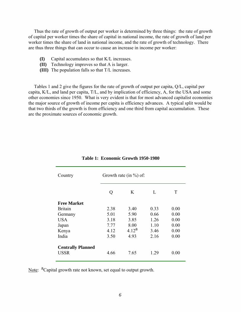
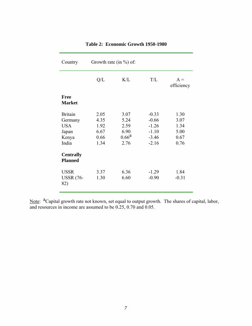
Thus the rate of growth of output per worker is determined by three things: the rate of growth of capital per worker times the share of capital in national income, the rate of growth of land per worker times the share of land in national income, and the rate of growth of technology. There are thus three things that can occur to cause an increase in income per worker: (I) Capital accumulates so that K/L increases. (II) Technology improves so that A is larger. (III) The population falls so that T/L increases. Tables 1 and 2 give the figures for the rate of growth of output per capita, Q/L, capital per capita, K/L, and land per capita, T/L, and by implication of efficiency, A, for the USA and some other economies since 1950. What is very evident is that for most advanced capitalist economies the major source of growth of income per capita is efficiency advances. A typical split would be that two thirds of the growth is from efficiency and one third from capital accumulation. These are the proximate sources of economic growth.

Table 1: Economic Growth 1950-1980

Growth rate (in %) of:

Country

Q K L T Free Market Britain 2.38 3.40 0.33 0.00 Germany 5.01 5.90 0.66 0.00 USA 3.18 3.85 1.26 0.00 Japan 7.77 8.00 1.10 0.00 Kenya 4.12 4.12a 3.46 0.00 India 3.50 4.93 2.16 0.00 Centrally Planned USSR

4.66 7.65 1.29 0.00

Note: aCapital growth rate not known, set equal to output growth.

7

Table 2: Economic Growth 1950-1980

Country

Growth rate (in %) of:

Q/L K/L T/L A =

efficiency Free Market

Britain 2.05 3.07 -0.33 1.30 Germany 4.35 5.24 -0.66 3.07 USA 1.92 2.59 -1.26 1.34 Japan 6.67 6.90 -1.10 5.00 Kenya 0.66 0.66a -3.46 0.67 India 1.34 2.76 -2.16 0.76 Centrally Planned

USSR 3.37 6.36 -1.29 1.84 USSR (76-82)

1.30 6.60 -0.90 -0.31

Note: aCapital growth rate not known, set equal to output growth. The shares of capital, labor, and resources in income are assumed to be 0.25, 0.70 and 0.05.

8

Using the growth accounting formulas Below I give some simple examples of growth accounting calculations. If you want to understand the equations given above your should work through these. 1. Suppose that in an economy a = 0.3, b = 0.5, and c = 0.2. Suppose that the growth of employment gL = 1%, the growth of capital gK is 5%, the growth of land gT = 0%, and the growth of technology gA = 2%. (a) What is the rate of growth of capital per worker and land per worker? (b) What is the rate of growth of output per worker? Answers (a) Growth rate of capital per worker is gK – gL = 5% – 1% = 4% Growth rate of land per worker is gT – gL = 0% – 1% = –1% (b) Growth rate of output per worker is, gQ – gL = a(gK – gL) + c(gT – gL) + gA = 0.3x4% + 0.2x(–1%) + 2% = 3% 2. Suppose that gQ = 3%, gK = 4%, gL = 1%, gT = 1%, and a = 1/3, b = 1/3, and c = 1/3. (a) What is the rate of growth of output per worker, capital per worker and land per worker? (b) What is the rate of growth of technology, gA? Answers (a) gQ – gL = 3% – 1% = 2% gK – gL = 4% – 1% = 3% gT – gL = 1% – 1% = 0% (b) gA = gQ – a.gK – b.gL – c.gT

= 3% – (1/3).4% – (1/3).1% – (1/3).1% = 1% 3. Suppose that the rate of growth of output, capital, labor and land in the same. What is the rate of growth of (a) output per worker? (b) technology? Answers (a) 0%, (b) 0%.

9

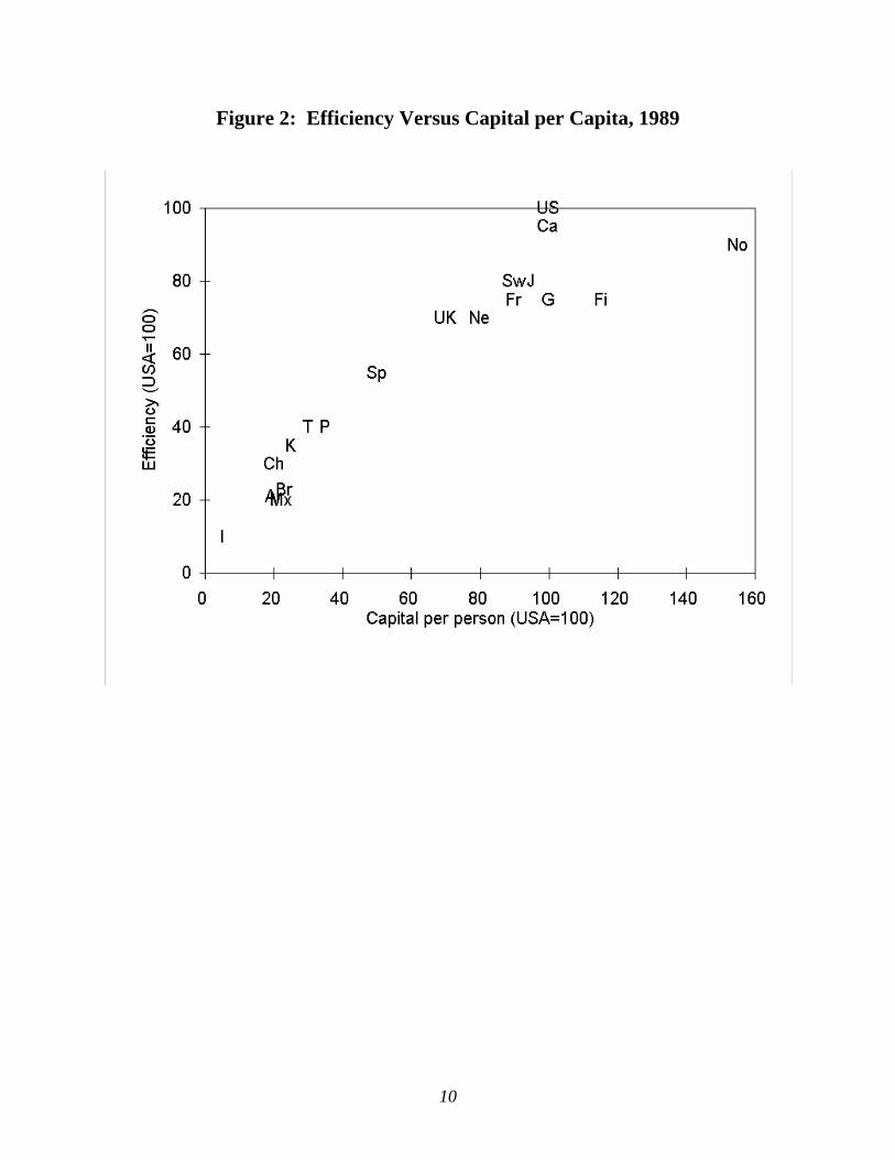
4. Suppose that gQ = 4%, gL = 2%, gK = 10%, gT = 0%, and a = 0.4, b = 0.4. What are (a) the rate of growth of output per worker and (b) the rate of growth of efficiency? Answers (a) 2%, (b) –0.8%. The Fundamental Source of Economic Growth If we plot on a diagram, however, the level of efficiency on the horizontal axis and the stock of capital per worker on the vertical axis, as is done in figure 2, we find a very close association between efficiency and the level of the capital stock. Countries with rapid growth of income per capita such as Japan have high rates of growth of efficiency and high rates of growth of capital per worker. Countries with low growth rates of income per capita have low rates of growth of efficiency and of capital per worker. This close association implies either that only one thing – efficiency or capital accumulation – must be the fundamental source of growth, or there must be some other factor which determines both efficiency and the capital stock that underlies modern economic growth. There has been vigorous and continuing debate among economists about what is this single underlying source of modern economic growth. Efficiency as the Fundamental Source of Growth Some would argue that efficiency growth can easily explain capital accumulation and that hence efficiency growth is the fundamental force. To understand the link consider that any gain in efficiency for a given stock of capital, labor and land in an economy will increase the marginal product of capital. The marginal product of capital from equation (1) is

Where ∆F/∆K is the change in F(K, L, T) produced by a one unit increase in K. By definition ∆F/∆K does not change when the level of efficiency A increases. Thus as A increases the marginal product of capital increases.

KTLKFAmpK ∆

∆⋅=

),,(

10

Figure 2: Efficiency Versus Capital per Capita, 1989

11

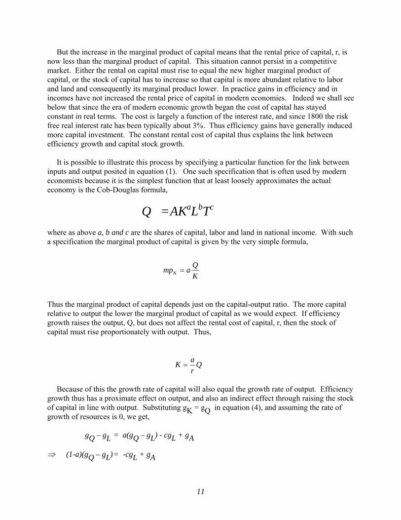
But the increase in the marginal product of capital means that the rental price of capital, r, is now less than the marginal product of capital. This situation cannot persist in a competitive market. Either the rental on capital must rise to equal the new higher marginal product of capital, or the stock of capital has to increase so that capital is more abundant relative to labor and land and consequently its marginal product lower. In practice gains in efficiency and in incomes have not increased the rental price of capital in modern economies. Indeed we shall see below that since the era of modern economic growth began the cost of capital has stayed constant in real terms. The cost is largely a function of the interest rate, and since 1800 the risk free real interest rate has been typically about 3%. Thus efficiency gains have generally induced more capital investment. The constant rental cost of capital thus explains the link between efficiency growth and capital stock growth. It is possible to illustrate this process by specifying a particular function for the link between inputs and output posited in equation (1). One such specification that is often used by modern economists because it is the simplest function that at least loosely approximates the actual economy is the Cob-Douglas formula,

Q = AKaLbTc where as above a, b and c are the shares of capital, labor and land in national income. With such a specification the marginal product of capital is given by the very simple formula,

Thus the marginal product of capital depends just on the capital-output ratio. The more capital relative to output the lower the marginal product of capital as we would expect. If efficiency growth raises the output, Q, but does not affect the rental cost of capital, r, then the stock of capital must rise proportionately with output. Thus,

Because of this the growth rate of capital will also equal the growth rate of output. Efficiency

growth thus has a proximate effect on output, and also an indirect effect through raising the stock of capital in line with output. Substituting gK = gQ in equation (4), and assuming the rate of growth of resources is 0, we get,

gQ – gL = a(gQ – gL) - cgL + gA ⇒ (1-a)(gQ – gL) = -cgL + gA

KQampK =

QraK =

12

⇒ gQ – gL = –[a/(1-a)]gL + gA/(1-a) (5) Now we see that the growth of income per capita depends on only two things. The rate of growth of population gL, and the rate of growth of technology gA. Also a 1% growth in efficiency leads to a more than 1% growth in output. If the share of capital in income is .25 for example, a 1% increase in efficiency will create a 1.33% growth in output. Thus at a deeper level efficiency explains not just the majority of economic growth; it explains almost all growth in output per person in the modern world, since income growth from efficiency gains also explains most of the capital accumulation.3 On this interpretation there is only one truly fundamental source of modern economic growth which is efficiency growth. Efficiency growth drives everything else. Capital as the Fundamental Source of Growth Despite the seemingly impeccable logic of the above argument, many economists have been troubled by the idea of imputing all growth to advances in efficiency. For where does this efficiency advance come from? Why is it occurring at a faster rate in some periods than others? This argument removes efficiency gains from the economic system altogether. It determines everything, but economists have nothing to say about it. Alternatively some economists have argued that all efficiency growth is really a form of capital investment. The argument is that efficiency growth does not occur as just a present from the Gods. It is brought about by people investing time and money in searching for new techniques and more cost effective ways of doing things. This search activity is as much capital investment as building a factory. If there is more efficiency growth in the modern world than before it must be because much more of this type of investment is occurring than before. Now the measured capital stock of societies does include the investments firms make in R&D. So in that case why does our basic accounting equation in growth accounting,

not show that none of the change in output comes from ∆A but most instead comes from ∆K? The answer, it is argued, is that capital investment in increasing knowledge has external benefits which are not captured by the investor. An external benefit of any action by an economic agent is a benefit that is not received by the actor. Thus if I paint my house I get benefits, but so do my neighbors even though they paid nothing. If I choose not to drive my car to work then by reducing congestion on the roads I give a benefit to all the other drivers that morning, but I receive no reward for these benefits. Suppose I invest in research and 3 The failure of efficiency to grow rapidly in the years since 1973 has caused real income growth in the US to be at a relatively low rate since then. Thus even though we have had little unemployment in recent years real incomes have grown relatively slowly.

ATLKFTsLwKrQ ∆⋅+∆+∆+∆=∆ ),,(

13

development to produce a new product such as a new medicine. The private return I earn on my investment will typically be much lower than the social return. For I can only patent my invention for a limited period. After that it can be freely used by all. Also others having seen what I have discovered can often mimic my innovation and produce competing products not covered by my patent. Or suppose I invest in a new auto plant. I get a private return from the cars I sell. But there may be a social return I do not capture in the training and experience that my workers acquire, and which they then take to other firms. If this is true for a lot of investment then the growth accounting equation we started with above will mislead us. For a true contribution of increases in the capital stock to output increases will be much greater than r.∆K, which merely measures the private benefits, and the contribution of efficiency gains F(K,L,T).∆A will be correspondingly less. Consequently in the growth accounting equation, gQ = agK + bgL + cgT + gA we have to replace the observed share of capital a, with a new share a*, where a* > a, and hence a* + b + c > 1. If the true contribution of capital to economic growth is under-measured we can explain why there is a correlation between capital growth and efficiency growth. Where capital growth is large, the under-measurement of the contribution of capital will be greatest. Thus where the growth rate of capital is large the growth of efficiency will appear large. If most economic growth is going to stem from capital investment, however, then the true coefficient on capital, a*, has to be about 3 times the payments to capital as a share of national income. That is the social return from investing $1 in capital has to be three times as big as the private return, so the external benefits have to be three times as great as the private benefits. Note that most of the capital stock is not machinery but is housing, roads and other infrastructure. It is hard to imagine any huge external benefit from putting up more sheet rock. Thus it must be that the external benefits from a small share of investment in machinery and industrial processes would have to be very great: as much as $10 or more of social benefit from each $1 of private gain. Yet attempts to detect such externalities have in general found much lower spillover effects of investment in technological advance. For this reason I prefer the view that what is really fundamental in modern economic growth is technical change. This then drives up the capital stock, further increasing income per capita. This suggests that a key question about the Industrial Revolution in Europe will be why the rate of technical change was low for so long and then became much more rapid. Population and Living Standards We saw in chapter 2 that in the Malthusian Economy the key determinant of living standards in the long run is fertility behavior. In the modern economy higher fertility will still reduce incomes per capita with a given level of technical change, since it reduces the level of resources per person, as we see in equation (4) above. But modern Europe as we saw has very low population growth rates. In both Italy and Germany the natural growth rate of population is

14

negative. Without immigrants both these countries and a substantial number of others in Western Europe would now be experiencing population declines. Thus in modern Europe population growth places very little drag on the increase of incomes per capital resulting from technical change.

In contrast in some parts of Northern and Central Africa, and in the Middle East, the rate of

natural increase of population exceeds 3%. This more rapid population growth in countries where the share of income derived from natural resources can be much higher than in Western industrialized nations will act as a significant reducer of the growth of incomes per capita. If, or example, resources and capital both constitute 25% of national income, then a population increase of 3% per year implies from equation (5) that the rate of increase of efficiency has to be 0.75% per year just to prevent output per person from falling. Thus, since gQ – gL = –[c/(1-a)]gL + gA/(1-a) If we want to ensure gQ – gL>0, we must have

-cgL + gA > 0 ⇒ gA > cgL ⇒ gA > 0.75%

Thus another important component in increasing living standards since the Industrial Revolution in the richer countries has been important demographic changes.

15

Estimating Efficiency Growth from Prices We showed above that the growth rate of efficiency can be calculated from the formula

gA = gQ – a.gK – b.gL – c.gT This method of calculating efficiency growth implies constructing measures of the movement over time of physical outputs, and weighting them by some estimate of the shares of each input in national income. Constructing such indices requires a lot of information about economies – we need to add up all the inputs and outputs for each economy. For most economies before 1850 or even 1900 it is impossible to get the required information to construct such measures of output growth. There is another method of calculating efficiency growth, however, which is much less information intensive. This is to construct measures of prices and payments to factors. If there is a competitive market knowing just a few prices will tell us what the general price level for any good or factor is. And such information can be obtained in economies such as England all the way back to 1250 or earlier. The basis of this alternative method is just the fact already noted that the value of output has to equal the value of inputs. Thus p.Q = rK + wL + sT (6) From year to year the quantities Q, K etc. and the prices p, r, etc. all change. Let the quantities next year be Q+∆Q, K+∆K, etc and the prices p+∆p, r+∆r, etc. Though all of these can and will change it must still be the case next year that the value of output, which is now (p + ∆p)(Q + ∆Q) must equal the value of the inputs. Thus (p + ∆p)(Q + ∆Q) = (r + ∆r)(K + ∆K) + (w + ∆w)(L + ∆L) + (s + ∆s)(T + ∆T) (7) If we subtract each side of (6) from each side of (7) and throw out the terms such as ∆p.∆Q which will be very small, then we get ∆p.Q + p.∆Q = ∆r.K + r.∆K + ∆w.L + w.∆L + ∆s.T + s.∆T Taking all the terms with quantity changes to the left hand side gives us p.∆Q – r.∆K – w.∆L – s.∆T = ∆r.K + ∆w.L + ∆s.T – ∆p.Q Dividing both sides by p.Q and rearranging we get,

16

⇒ gQ – a.gK – b.gL – c.gT = a.gr + b.gw + c.gs – gp But as we noted above,

gA = gQ – a.gK – b.gL – c.gT In consequence it must also be the case that gA = a.gr + b.gw + c.gs – gp (8) The implication of this equation is that the rate of productivity growth can be calculated in two different ways: as the rate of growth of output minus the weighted rate of growth of the inputs, or as the weighted sum of the rates of growth of input prices minus the rate of growth of the output price. Suppose, for example, the cost of capital, wages, and land rents are all growing at 5%, but the price of output is growing at 2%. Then the rate of productivity growth is gA = α×.05 + β×.05 + γ×.05 – .02 = .05 - .02 = 3%. Equation (8) can also be rewritten as: gA = a.(gr – gp) + b.(gw – gp) + c.(gs– gp) = a.gr/p + b.gw/p + c.gs/p

This says that the rate of efficiency growth is the weighted sum of the rate of growth of real capital rents, real wages and real land rents. Now since as we saw real capital rents have tended to be constant since 1750, and real land rents have not grown very rapidly, what this implies is that the real wages of workers tend to be for modern economies a very good metric of the efficiency level of the economy. Most efficiency growth in modern economies has shown up in higher real wages.

pp

ssc

wwb

rra

TTc

LLb

KKa

QQ ∆

−∆

+∆

+∆

=∆

+∆

+∆

−∆

17

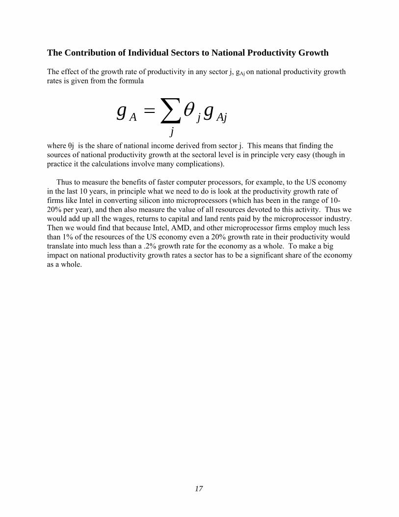
The Contribution of Individual Sectors to National Productivity Growth The effect of the growth rate of productivity in any sector j, gAj on national productivity growth rates is given from the formula

∑=j

AjjA gg θ

where θj is the share of national income derived from sector j. This means that finding the sources of national productivity growth at the sectoral level is in principle very easy (though in practice it the calculations involve many complications).

Thus to measure the benefits of faster computer processors, for example, to the US economy in the last 10 years, in principle what we need to do is look at the productivity growth rate of firms like Intel in converting silicon into microprocessors (which has been in the range of 10-20% per year), and then also measure the value of all resources devoted to this activity. Thus we would add up all the wages, returns to capital and land rents paid by the microprocessor industry. Then we would find that because Intel, AMD, and other microprocessor firms employ much less than 1% of the resources of the US economy even a 20% growth rate in their productivity would translate into much less than a .2% growth rate for the economy as a whole. To make a big impact on national productivity growth rates a sector has to be a significant share of the economy as a whole.

18

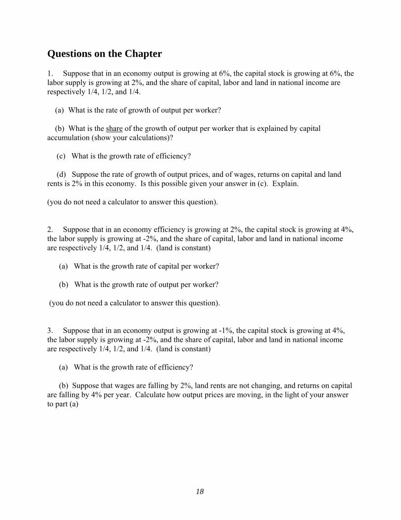
Questions on the Chapter 1. Suppose that in an economy output is growing at 6%, the capital stock is growing at 6%, the labor supply is growing at 2%, and the share of capital, labor and land in national income are respectively 1/4, 1/2, and 1/4. (a) What is the rate of growth of output per worker? (b) What is the share of the growth of output per worker that is explained by capital accumulation (show your calculations)?

(c) What is the growth rate of efficiency?

(d) Suppose the rate of growth of output prices, and of wages, returns on capital and land rents is 2% in this economy. Is this possible given your answer in (c). Explain. (you do not need a calculator to answer this question). 2. Suppose that in an economy efficiency is growing at 2%, the capital stock is growing at 4%, the labor supply is growing at -2%, and the share of capital, labor and land in national income are respectively 1/4, 1/2, and 1/4. (land is constant) (a) What is the growth rate of capital per worker? (b) What is the growth rate of output per worker? (you do not need a calculator to answer this question). 3. Suppose that in an economy output is growing at -1%, the capital stock is growing at 4%, the labor supply is growing at -2%, and the share of capital, labor and land in national income are respectively 1/4, 1/2, and 1/4. (land is constant) (a) What is the growth rate of efficiency? (b) Suppose that wages are falling by 2%, land rents are not changing, and returns on capital are falling by 4% per year. Calculate how output prices are moving, in the light of your answer to part (a)

19

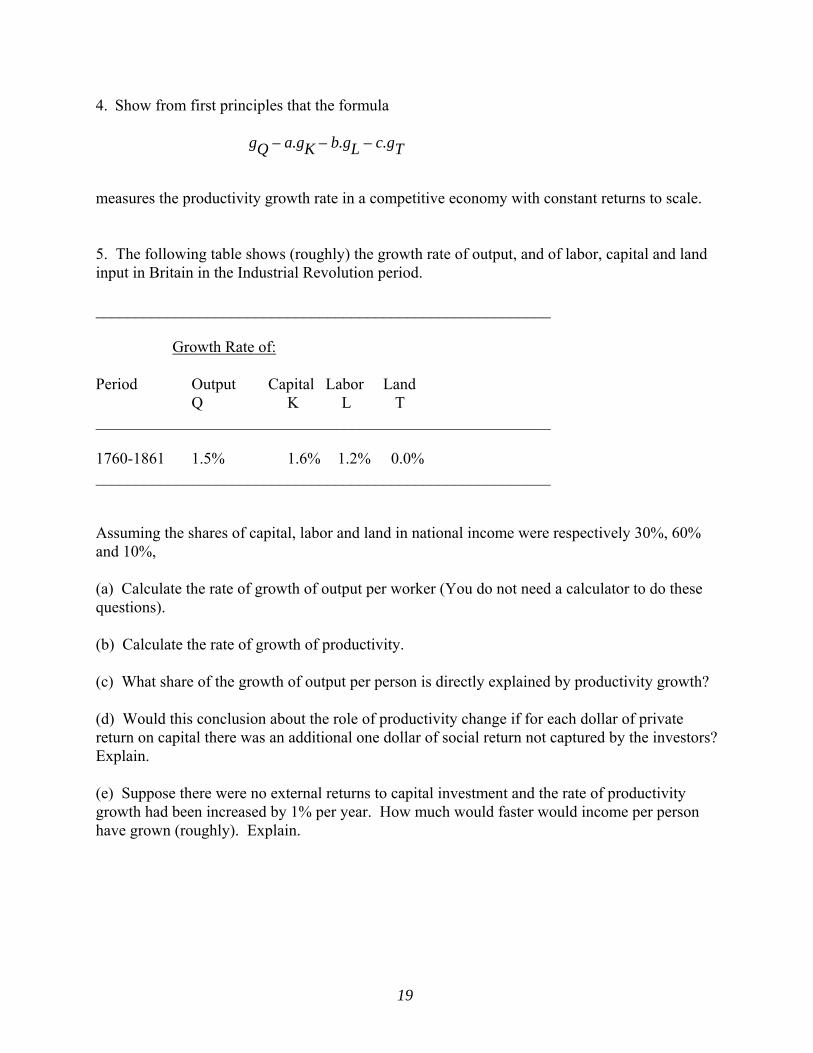
4. Show from first principles that the formula gQ – a.gK – b.gL – c.gT measures the productivity growth rate in a competitive economy with constant returns to scale. 5. The following table shows (roughly) the growth rate of output, and of labor, capital and land input in Britain in the Industrial Revolution period. _________________________________________________________

Growth Rate of:

Period Output Capital Labor Land

Q K L T _________________________________________________________

1760-1861 1.5% 1.6% 1.2% 0.0% _________________________________________________________

Assuming the shares of capital, labor and land in national income were respectively 30%, 60% and 10%, (a) Calculate the rate of growth of output per worker (You do not need a calculator to do these questions). (b) Calculate the rate of growth of productivity. (c) What share of the growth of output per person is directly explained by productivity growth? (d) Would this conclusion about the role of productivity change if for each dollar of private return on capital there was an additional one dollar of social return not captured by the investors? Explain. (e) Suppose there were no external returns to capital investment and the rate of productivity growth had been increased by 1% per year. How much would faster would income per person have grown (roughly). Explain.

20

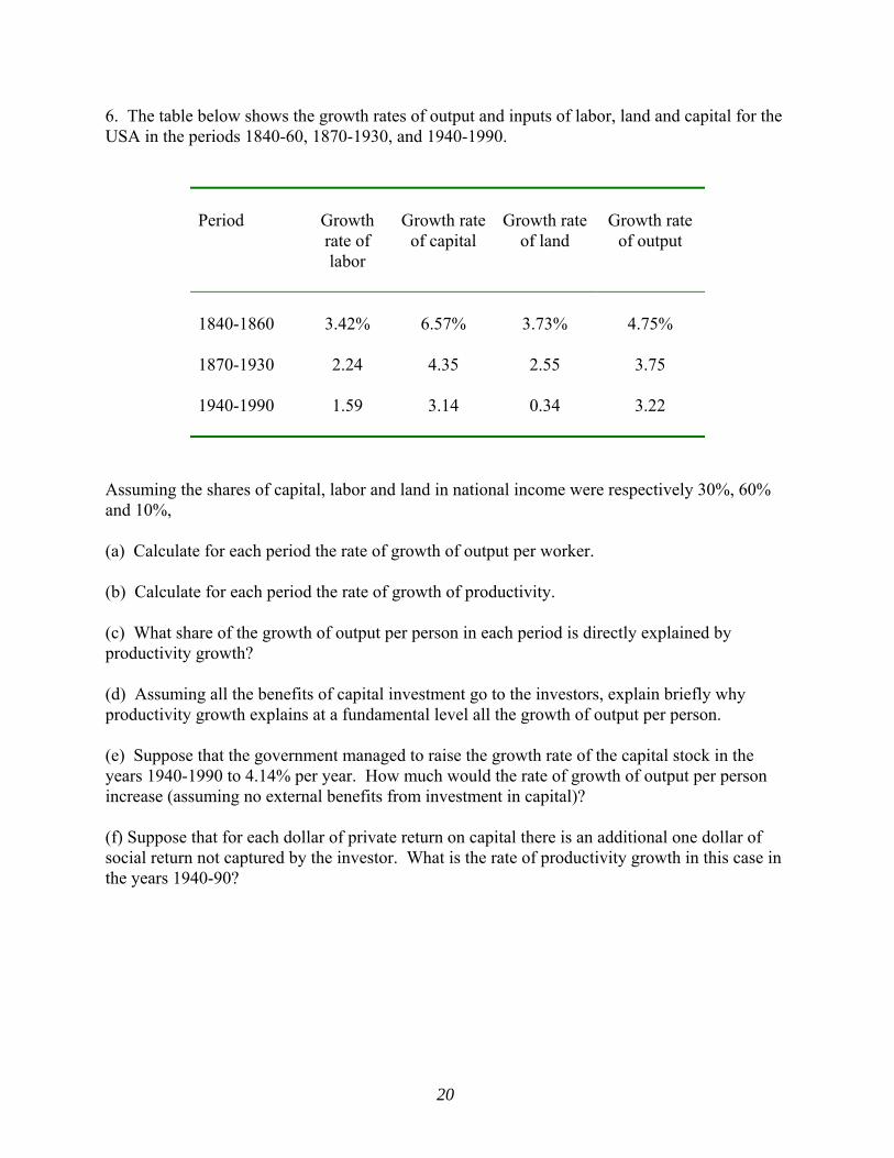
6. The table below shows the growth rates of output and inputs of labor, land and capital for the USA in the periods 1840-60, 1870-1930, and 1940-1990.

Period

Growth rate of labor

Growth rate

of capital

Growth rate

of land

Growth rate

of output

1840-1860 3.42% 6.57% 3.73% 4.75% 1870-1930 2.24 4.35 2.55 3.75 1940-1990 1.59 3.14 0.34 3.22

Assuming the shares of capital, labor and land in national income were respectively 30%, 60% and 10%, (a) Calculate for each period the rate of growth of output per worker. (b) Calculate for each period the rate of growth of productivity. (c) What share of the growth of output per person in each period is directly explained by productivity growth? (d) Assuming all the benefits of capital investment go to the investors, explain briefly why productivity growth explains at a fundamental level all the growth of output per person. (e) Suppose that the government managed to raise the growth rate of the capital stock in the years 1940-1990 to 4.14% per year. How much would the rate of growth of output per person increase (assuming no external benefits from investment in capital)? (f) Suppose that for each dollar of private return on capital there is an additional one dollar of social return not captured by the investor. What is the rate of productivity growth in this case in the years 1940-90?

21

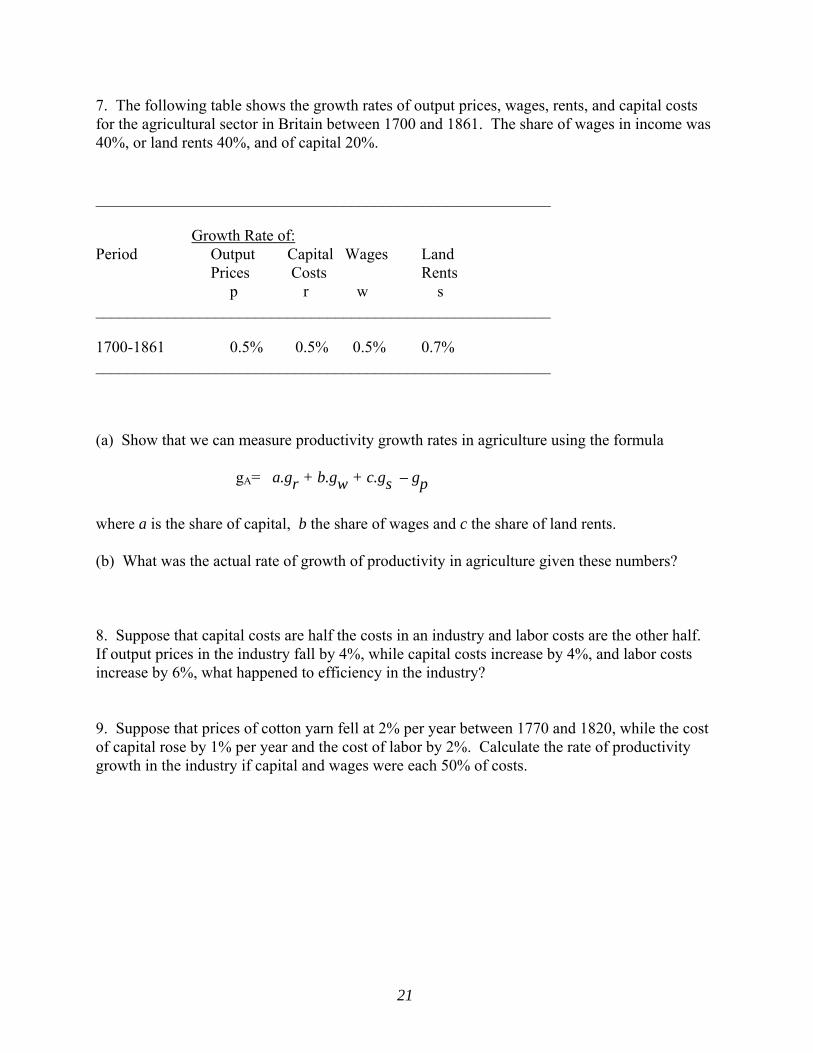
7. The following table shows the growth rates of output prices, wages, rents, and capital costs for the agricultural sector in Britain between 1700 and 1861. The share of wages in income was 40%, or land rents 40%, and of capital 20%. _________________________________________________________

Growth Rate of:

Period Output Capital Wages Land Prices Costs Rents p r w s

_________________________________________________________

1700-1861 0.5% 0.5% 0.5% 0.7% _________________________________________________________ (a) Show that we can measure productivity growth rates in agriculture using the formula gA= a.gr + b.gw + c.gs – gp

where a is the share of capital, b the share of wages and c the share of land rents. (b) What was the actual rate of growth of productivity in agriculture given these numbers? 8. Suppose that capital costs are half the costs in an industry and labor costs are the other half. If output prices in the industry fall by 4%, while capital costs increase by 4%, and labor costs increase by 6%, what happened to efficiency in the industry? 9. Suppose that prices of cotton yarn fell at 2% per year between 1770 and 1820, while the cost of capital rose by 1% per year and the cost of labor by 2%. Calculate the rate of productivity growth in the industry if capital and wages were each 50% of costs.