1
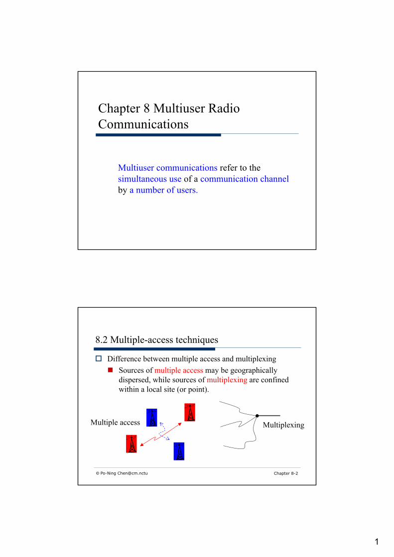
Chapter 8 Multiuser Radio Communications
Multiuser communications refer to thesimultaneous use of a communication channel by a number of users.
© Po-Ning [email protected] Chapter 8-2
8.2 Multiple-access techniques
o Difference between multiple access and multiplexingn Sources of multiple access may be geographically
dispersed, while sources of multiplexing are confined within a local site (or point).
MultiplexingMultiple access
2
© Po-Ning [email protected] Chapter 8-3
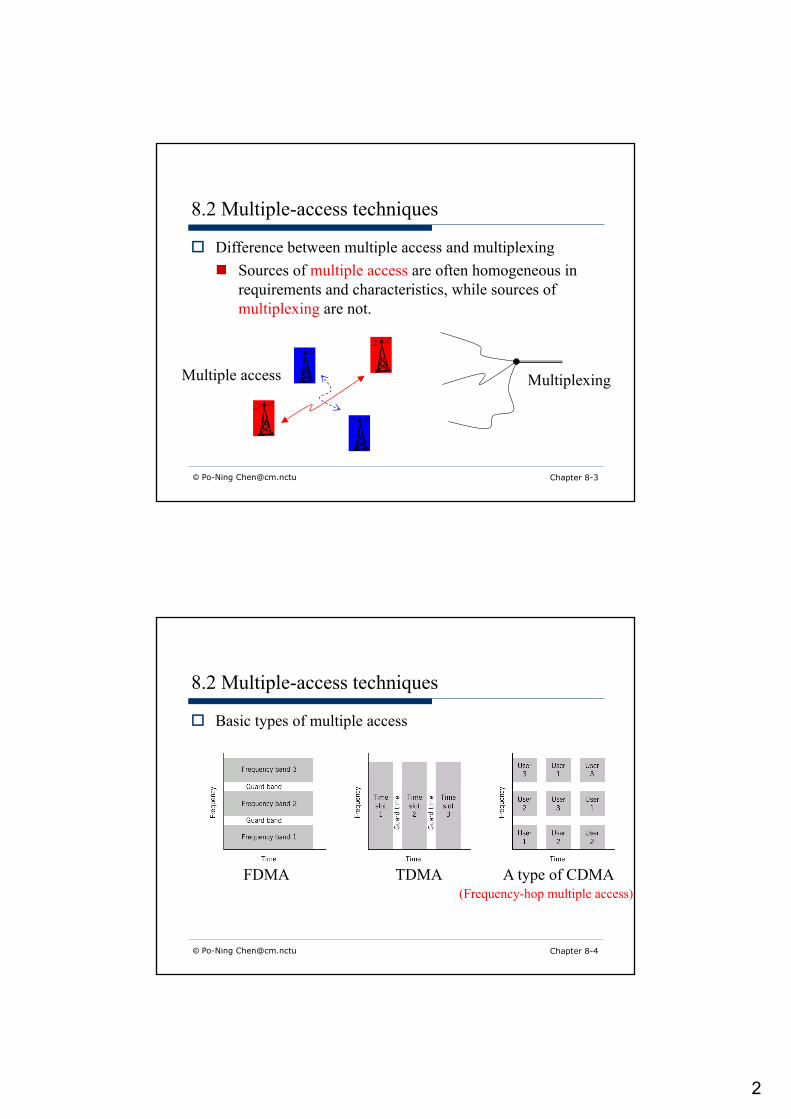
8.2 Multiple-access techniques
o Difference between multiple access and multiplexingn Sources of multiple access are often homogeneous in
requirements and characteristics, while sources of multiplexing are not.
MultiplexingMultiple access
© Po-Ning [email protected] Chapter 8-4
8.2 Multiple-access techniques
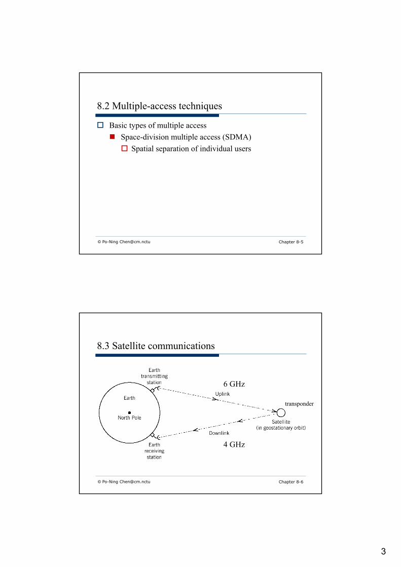
o Basic types of multiple access
FDMA TDMA A type of CDMA(Frequency-hop multiple access)
3
© Po-Ning [email protected] Chapter 8-5
8.2 Multiple-access techniques
o Basic types of multiple accessn Space-division multiple access (SDMA)
o Spatial separation of individual users
© Po-Ning [email protected] Chapter 8-6
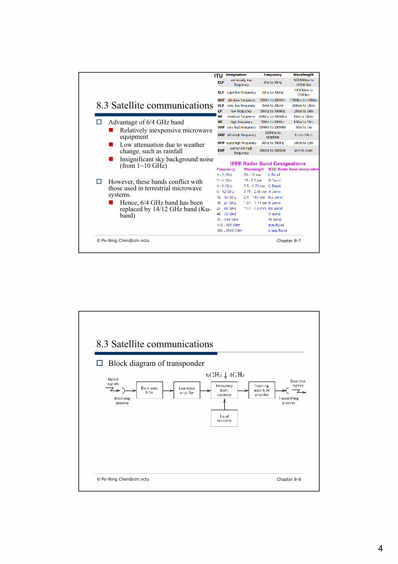
8.3 Satellite communications
6 GHz
4 GHz
transponder
4
© Po-Ning [email protected] Chapter 8-7
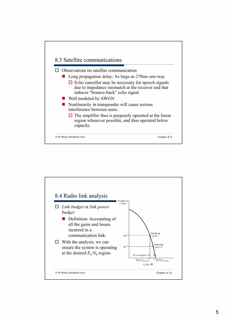
8.3 Satellite communicationso Advantage of 6/4 GHz band
n Relatively inexpensive microwave equipment
n Low attenuation due to weather change, such as rainfall
n Insignificant sky background noise (from 1~10 GHz)
o However, these bands conflict with those used in terrestrial microwave systems.n Hence, 6/4 GHz band has been
replaced by 14/12 GHz band (Ku-band)
ITU
© Po-Ning [email protected] Chapter 8-8
8.3 Satellite communications
o Block diagram of transponder
5
© Po-Ning [email protected] Chapter 8-9
8.3 Satellite communications
o Observations on satellite communicationn Long propagation delay: As large as 270ms one-way
o Echo canceller may be necessary for speech signals due to impedance mismatch at the receiver end that induces “bounce-back” echo signal.
n Well modeled by AWGNn Nonlinearity in transponder will cause serious
interference between users.o The amplifier thus is purposely operated at the linear
region whenever possible, and thus operated below capacity.
© Po-Ning [email protected] Chapter 8-10
8.4 Radio link analysis
o Link budget or link power budgetn Definition: Accounting of
all the gains and losses incurred in a communication link.
o With the analysis, we can ensure the system is operating at the desired Eb/N0 region.
6
© Po-Ning [email protected] Chapter 8-11
8.4 Radio link analysis
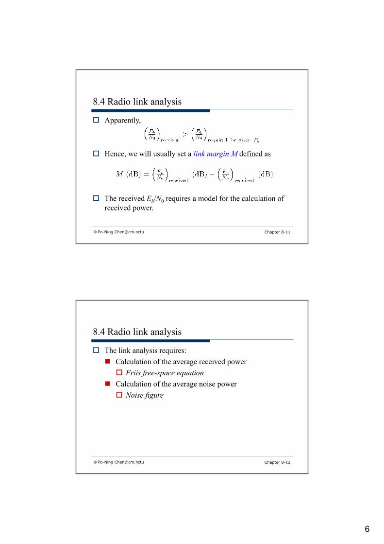
o Apparently,
o Hence, we will usually set a link margin M defined as
o The received Eb/N0 requires a model for the calculation of received power.
© Po-Ning [email protected] Chapter 8-12
8.4 Radio link analysis
o The link analysis requires:n Calculation of the average received power
o Friis free-space equationn Calculation of the average noise power
o Noise figure
7
© Po-Ning [email protected] Chapter 8-13
8.4 Radio link analysis
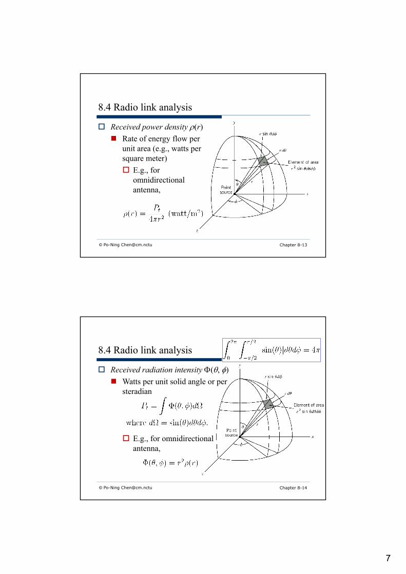
o Received power density r(r)n Rate of energy flow per
unit area (e.g., watts per square meter)o E.g., for
omnidirectional antenna,
© Po-Ning [email protected] Chapter 8-14
8.4 Radio link analysis
o Received radiation intensity F(q, f)n Watts per unit solid angle or per
steradian
o E.g., for omnidirectional antenna,
8
© Po-Ning [email protected] Chapter 8-15
8.4 Radio link analysis
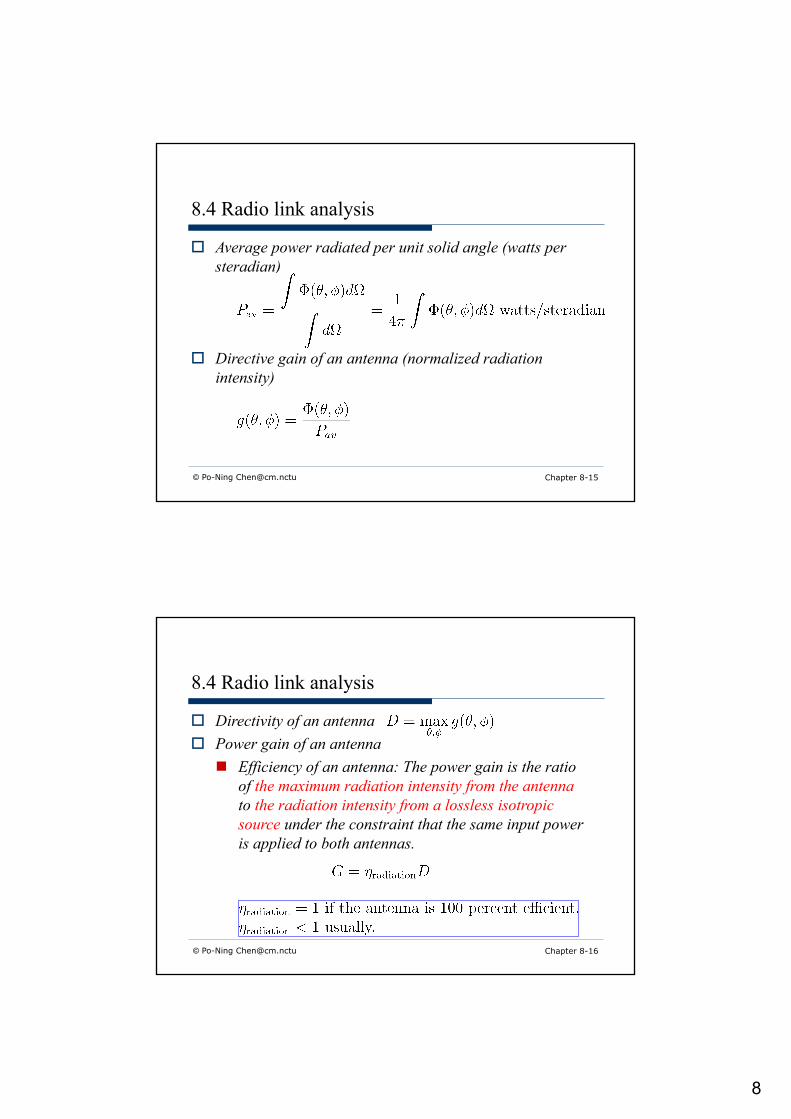
o Average power radiated per unit solid angle (watts per steradian)
o Directive gain of an antenna (normalized radiation intensity)
© Po-Ning [email protected] Chapter 8-16
8.4 Radio link analysis
o Directivity of an antennao Power gain of an antenna
n Efficiency of an antenna: The power gain is the ratio of the maximum radiation intensity from the antennato the radiation intensity from a lossless isotropic source under the constraint that the same input power is applied to both antennas.
9
© Po-Ning [email protected] Chapter 8-17
8.4 Radio link analysis
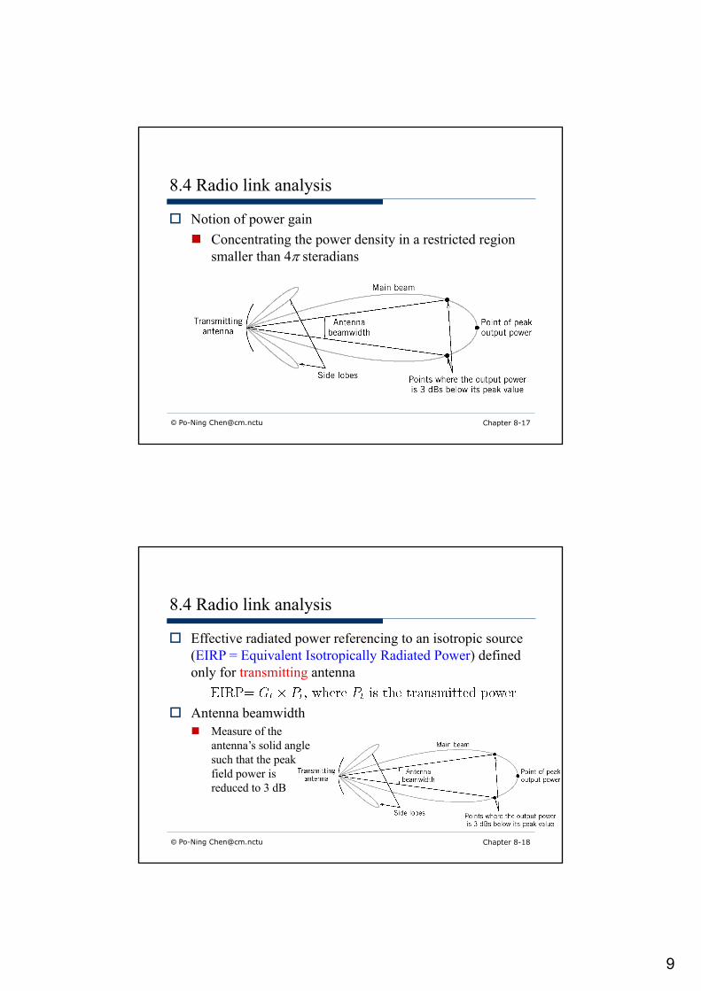
o Notion of power gainn Concentrating the power density in a restricted region
smaller than 4p steradians
© Po-Ning [email protected] Chapter 8-18
8.4 Radio link analysis
o Effective radiated power referencing to an isotropic source (EIRP = Equivalent Isotropically Radiated Power) defined only for transmitting antenna
o Antenna beamwidthn Measure of the
antenna’s solid angle such that the peak field power is reduced to 3 dB
10
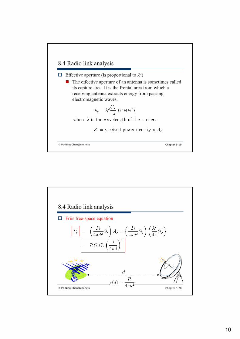
© Po-Ning [email protected] Chapter 8-19
8.4 Radio link analysis
o Effective aperture (is proportional to l2)n The effective aperture of an antenna is sometimes called
its capture area. It is the frontal area from which a receiving antenna extracts energy from passing electromagnetic waves.
© Po-Ning [email protected] Chapter 8-20
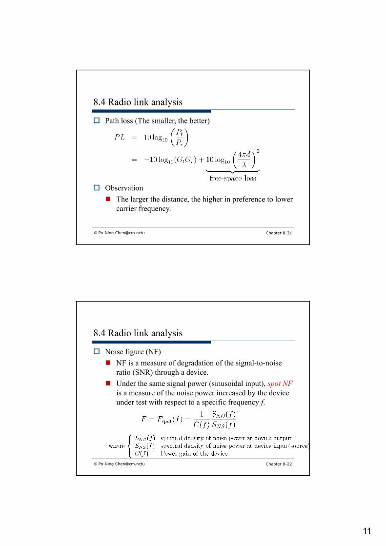
8.4 Radio link analysis
o Friis free-space equation
d
11
© Po-Ning [email protected] Chapter 8-21
8.4 Radio link analysis
o Path loss (The smaller, the better)
o Observationn The larger the distance, the higher in preference to lower
carrier frequency.
© Po-Ning [email protected] Chapter 8-22
8.4 Radio link analysis
o Noise figure (NF)n NF is a measure of degradation of the signal-to-noise
ratio (SNR) through a device.n Under the same signal power (sinusoidal input), spot NF
is a measure of the noise power increased by the device under test with respect to a specific frequency f.
12
© Po-Ning [email protected] Chapter 8-23
8.4 Radio link analysis
o With the above definition on G(f),
o Suppose we concern about the average noise figure. Then,
© Po-Ning [email protected] Chapter 8-24
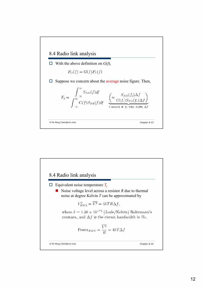
8.4 Radio link analysis
o Equivalent noise temperature Ten Noise voltage level across a resistor R due to thermal
noise at degree Kelvin T can be approximated by
13
© Po-Ning [email protected] Chapter 8-25
8.4 Radio link analysis
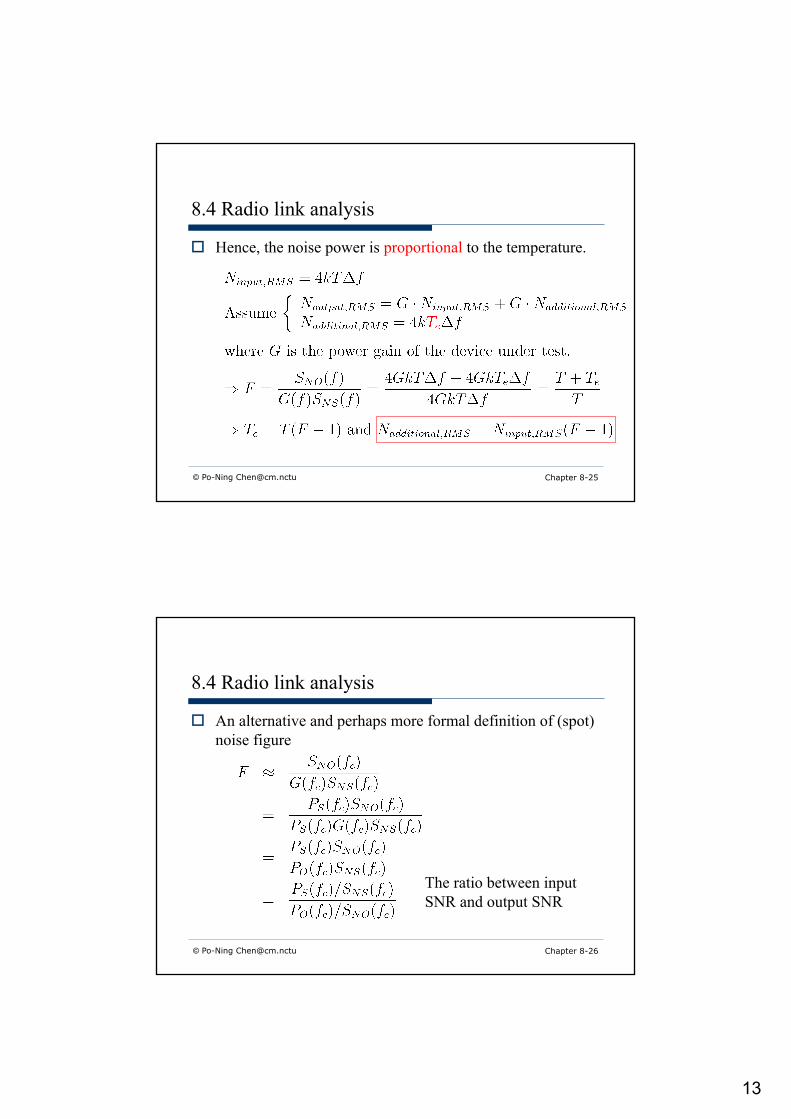
o Hence, the noise power is proportional to the temperature.
© Po-Ning [email protected] Chapter 8-26
8.4 Radio link analysis
o An alternative and perhaps more formal definition of (spot) noise figure
The ratio between input SNR and output SNR
14
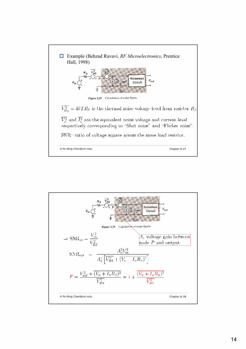
o Example (Behzad Ravavi, RF Microelectronics, Prentice Hall, 1998)
© Po-Ning [email protected] Chapter 8-27
© Po-Ning [email protected] Chapter 8-28
15
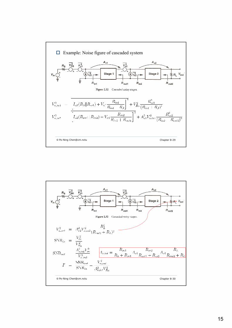
o Example: Noise figure of cascaded system
© Po-Ning [email protected] Chapter 8-29
© Po-Ning [email protected] Chapter 8-30
16
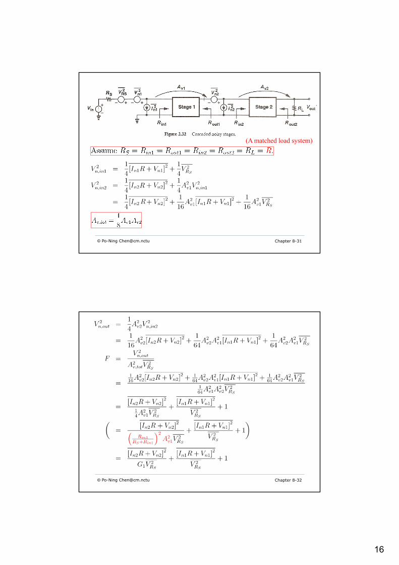
© Po-Ning [email protected] Chapter 8-31
(A matched load system)
© Po-Ning [email protected] Chapter 8-32
17
© Po-Ning [email protected] Chapter 8-33
o Note that F2 is the noise figure of the second stage with respect to a source impedance RS.
o Also, note that Rout1 = RS.o Generally,
© Po-Ning [email protected] Chapter 8-34
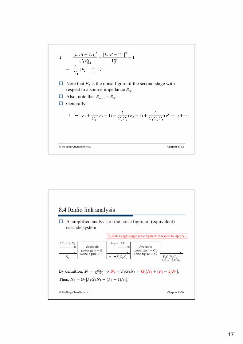
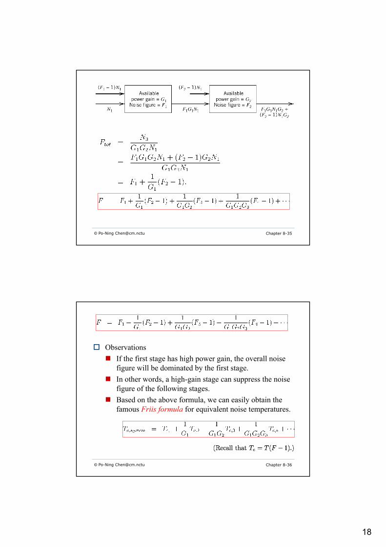
8.4 Radio link analysis
o A simplified analysis of the noise figure of (equivalent) cascade system
F2 is the (single-stage) noise figure with respect to input N1.
18
© Po-Ning [email protected] Chapter 8-35
o Observationsn If the first stage has high power gain, the overall noise
figure will be dominated by the first stage.n In other words, a high-gain stage can suppress the noise
figure of the following stages.n Based on the above formula, we can easily obtain the
famous Friis formula for equivalent noise temperatures.
© Po-Ning [email protected] Chapter 8-36
19
© Po-Ning [email protected] Chapter 8-37
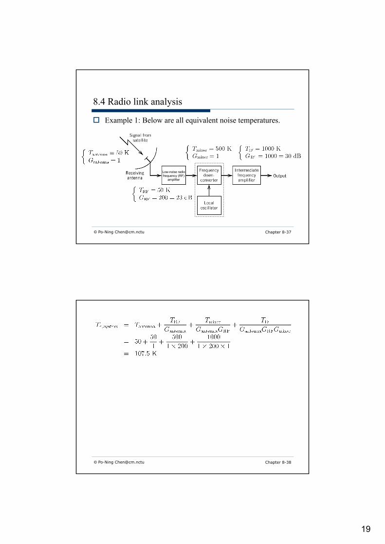
8.4 Radio link analysis
o Example 1: Below are all equivalent noise temperatures.
Low-noise radio frequency (RF)
amplifier
© Po-Ning [email protected] Chapter 8-38
20
© Po-Ning [email protected] Chapter 8-39
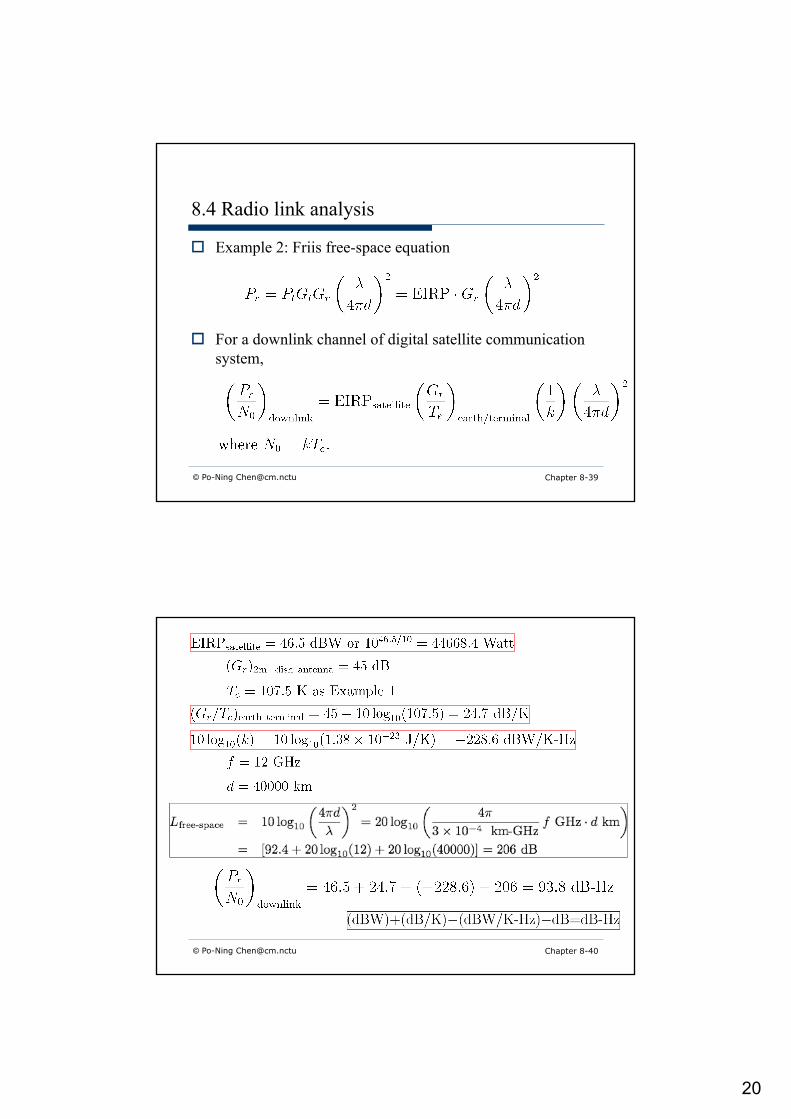
8.4 Radio link analysis
o Example 2: Friis free-space equation
o For a downlink channel of digital satellite communication system,
© Po-Ning [email protected] Chapter 8-40
21
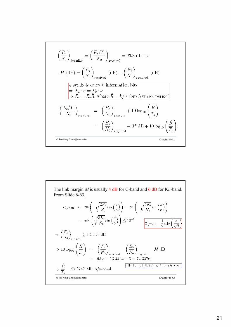
© Po-Ning [email protected] Chapter 8-41
© Po-Ning [email protected] Chapter 8-42
The link margin M is usually 4 dB for C-band and 6 dB for Ku-band.From Slide 6-63,
22
© Po-Ning [email protected] Chapter 8-43
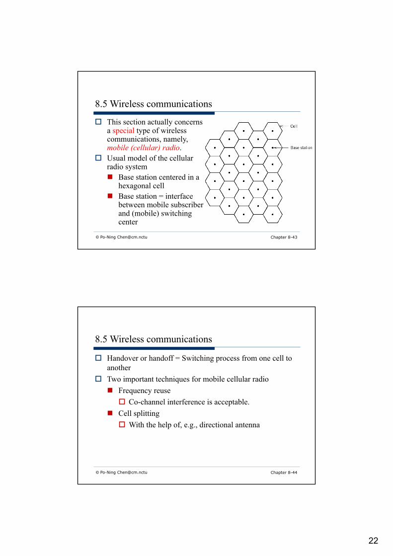
8.5 Wireless communications
o This section actually concerns a special type of wireless communications, namely, mobile (cellular) radio.
o Usual model of the cellular radio systemn Base station centered in a
hexagonal celln Base station = interface
between mobile subscriber and (mobile) switching center
© Po-Ning [email protected] Chapter 8-44
8.5 Wireless communications
o Handover or handoff = Switching process from one cell to another
o Two important techniques for mobile cellular radion Frequency reuse
o Co-channel interference is acceptable.n Cell splitting
o With the help of, e.g., directional antenna
23
© Po-Ning [email protected] Chapter 8-45
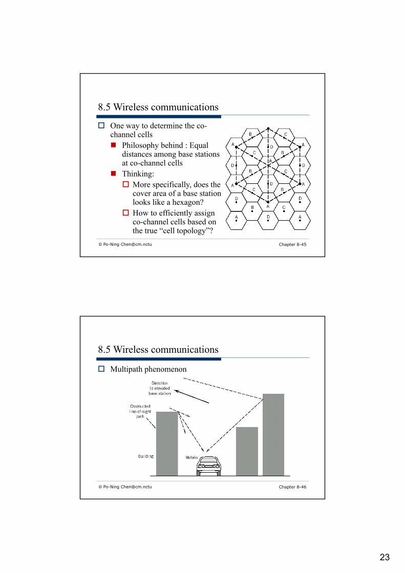
8.5 Wireless communications
o One way to determine the co-channel cellsn Philosophy behind : Equal
distances among base stations at co-channel cells
n Thinking: o More specifically, does the
cover area of a base station looks like a hexagon?
o How to efficiently assign co-channel cells based on the true “cell topology”?
© Po-Ning [email protected] Chapter 8-46
8.5 Wireless communications
o Multipath phenomenon
24
© Po-Ning [email protected] Chapter 8-47
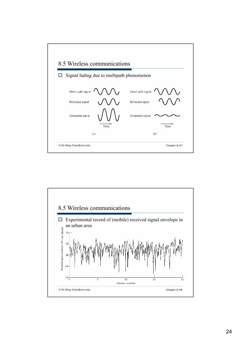
8.5 Wireless communications
o Signal fading due to multipath phenomenon
© Po-Ning [email protected] Chapter 8-48
8.5 Wireless communications
o Experimental record of (mobile) received signal envelope in an urban area
(OrdBm
W)
25
© Po-Ning [email protected] Chapter 8-49
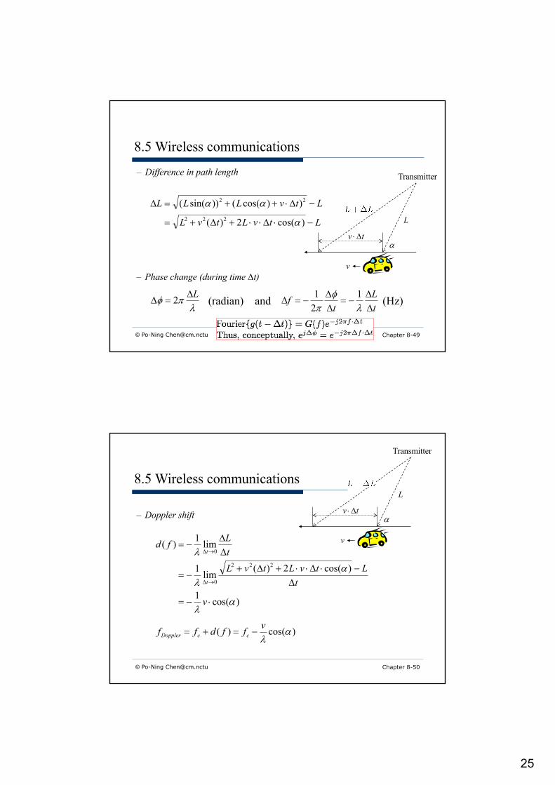
Transmitter
L
atv D×
v
LtvLtvL
LtvLLL
-×D××+D+=
-D×++=D
)cos(2)(
))cos(())sin((222
22
a
aa
– Difference in path length
8.5 Wireless communications
lpf LD
=D 2
– Phase change (during time Dt)
(radian) and tL
tf
DD
-=DD
-=Dl
fp
121
(Hz)
© Po-Ning [email protected] Chapter 8-50
Transmitter
L
atv D×
v
)cos(1
)cos(2)(lim
1
lim1)(
222
0
0
al
al
l
×-=
D-×D××+D+
-=
DD
-=
®D
®D
v
tLtvLtvL
tLfd
t
t
– Doppler shift
8.5 Wireless communications
)cos()( alvffdff ccDoppler -=+=
26
© Po-Ning [email protected] Chapter 8-51
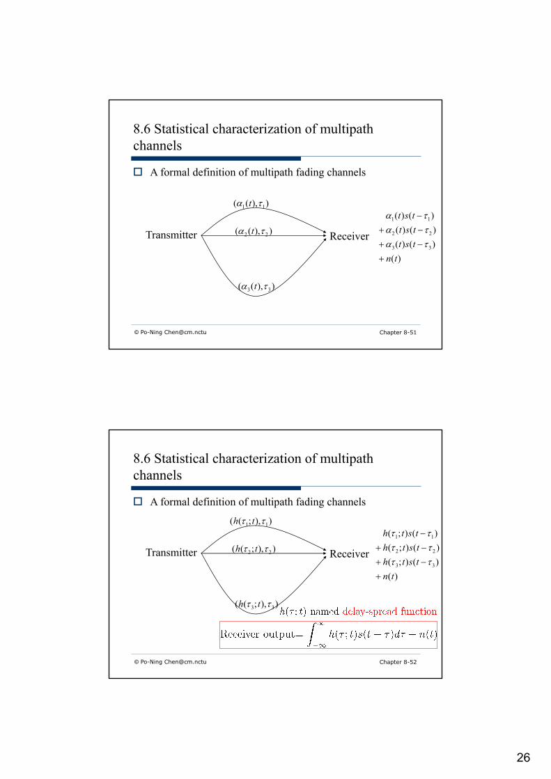
8.6 Statistical characterization of multipath channels
o A formal definition of multipath fading channels
Transmitter Receiver
)),(( 11 ta t
)),(( 22 ta t
)),(( 33 ta t
)()()()()()()(
33
22
11
tntsttsttst
+-+-+-
tatata
© Po-Ning [email protected] Chapter 8-52
8.6 Statistical characterization of multipath channels
o A formal definition of multipath fading channels
Transmitter Receiver
)),;(( 11 tt th
)),;(( 22 tt th
)),;(( 33 tt th
)()();()();()();(
33
22
11
tntsthtsthtsth
+-+-+-
tttttt
27
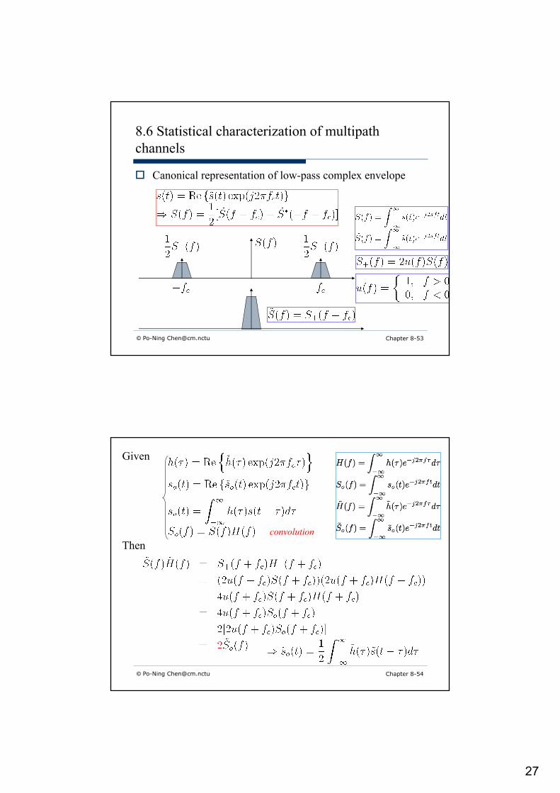
© Po-Ning [email protected] Chapter 8-53
8.6 Statistical characterization of multipath channels
o Canonical representation of low-pass complex envelope
Given
Then
© Po-Ning [email protected] Chapter 8-54
convolution
28
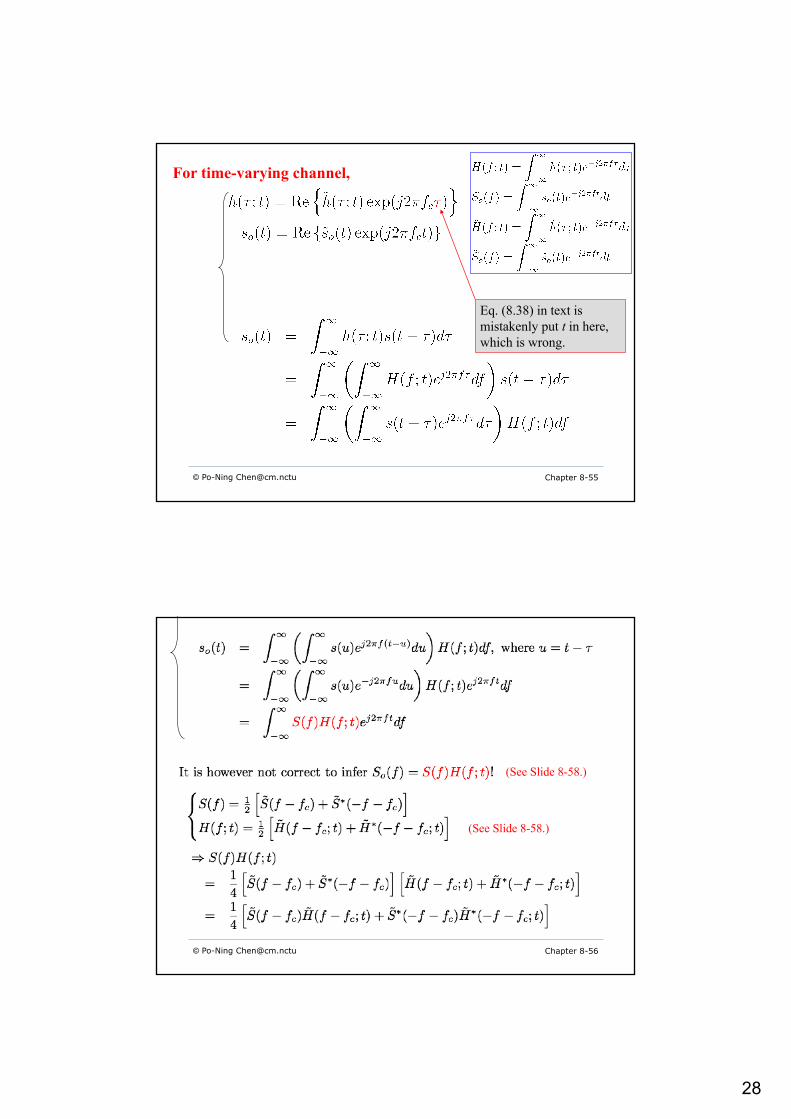
For time-varying channel,
© Po-Ning [email protected] Chapter 8-55
Eq. (8.38) in text is mistakenly put t in here, which is wrong.
© Po-Ning [email protected] Chapter 8-56
(See Slide 8-58.)
(See Slide 8-58.)
29
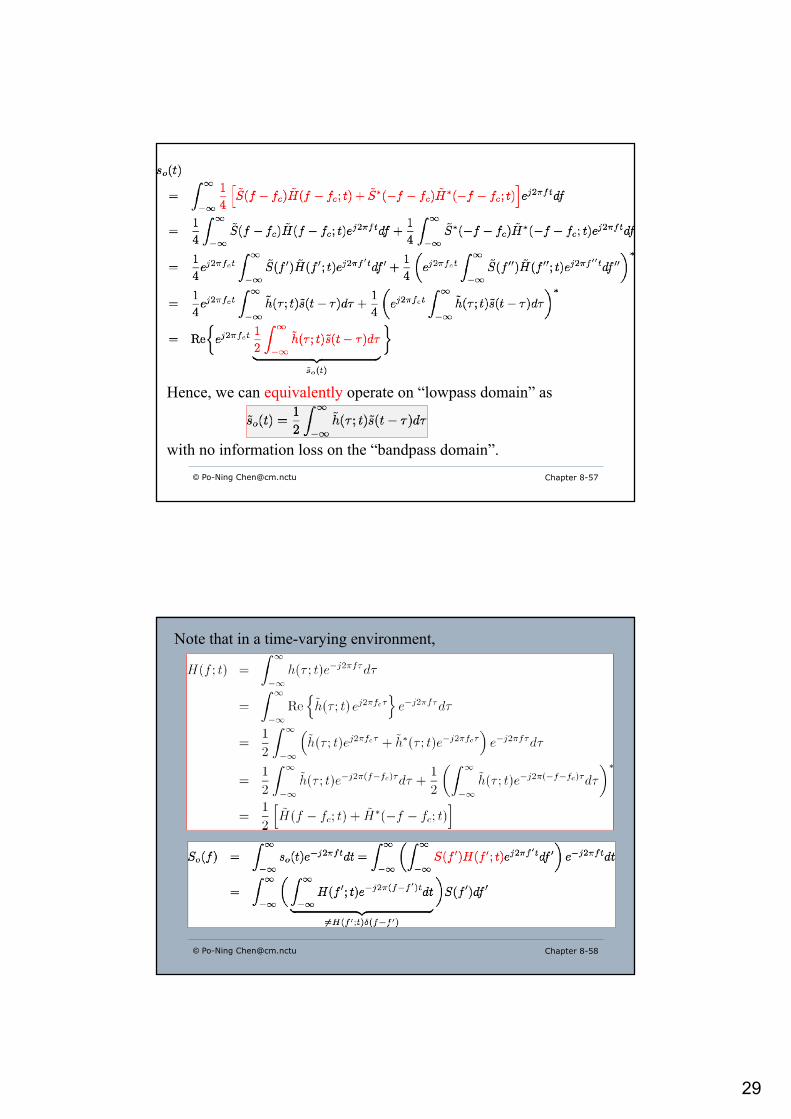
© Po-Ning [email protected] Chapter 8-57
Hence, we can equivalently operate on “lowpass domain” as
with no information loss on the “bandpass domain”.
© Po-Ning [email protected] Chapter 8-58
Note that in a time-varying environment,
30
© Po-Ning [email protected] Chapter 8-59
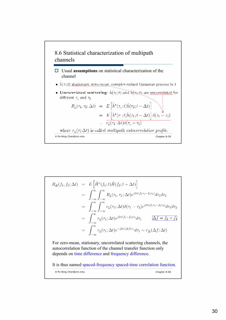
8.6 Statistical characterization of multipath channels
o Usual assumptions on statistical characterization of the channel
© Po-Ning [email protected] Chapter 8-60
For zero-mean, stationary, uncorrelated scattering channels, the autocorrelation function of the channel transfer function only depends on time difference and frequency difference.
It is thus named spaced-frequency spaced-time correlation function.
31
© Po-Ning [email protected] Chapter 8-61
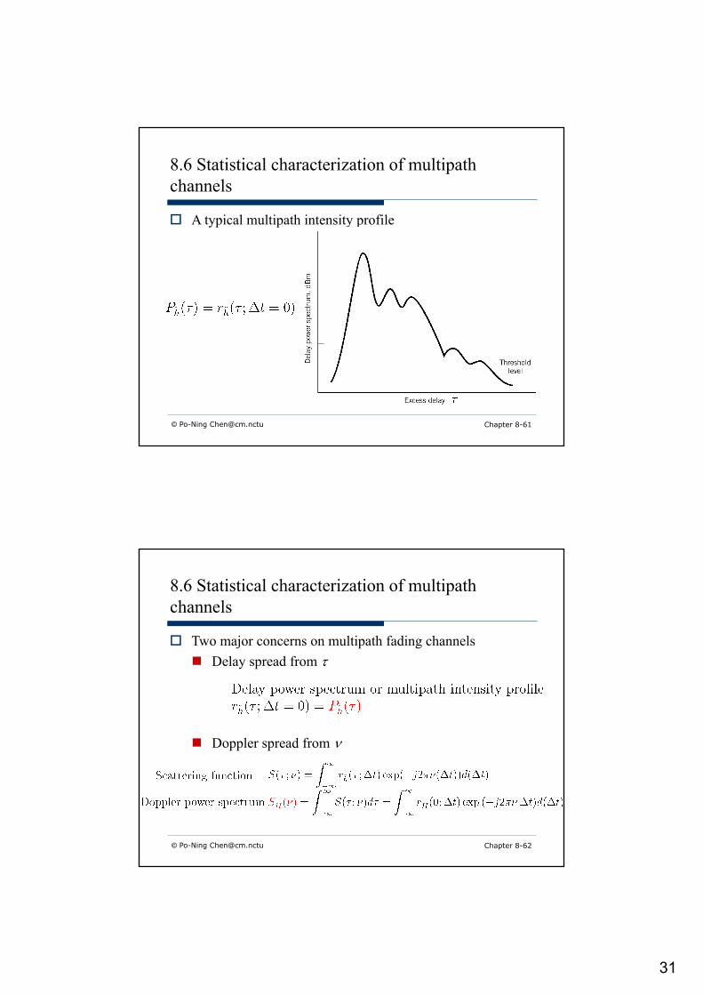
8.6 Statistical characterization of multipath channels
o A typical multipath intensity profile
© Po-Ning [email protected] Chapter 8-62
8.6 Statistical characterization of multipath channels
o Two major concerns on multipath fading channelsn Delay spread from t
n Doppler spread from n
32
© Po-Ning [email protected] Chapter 8-63
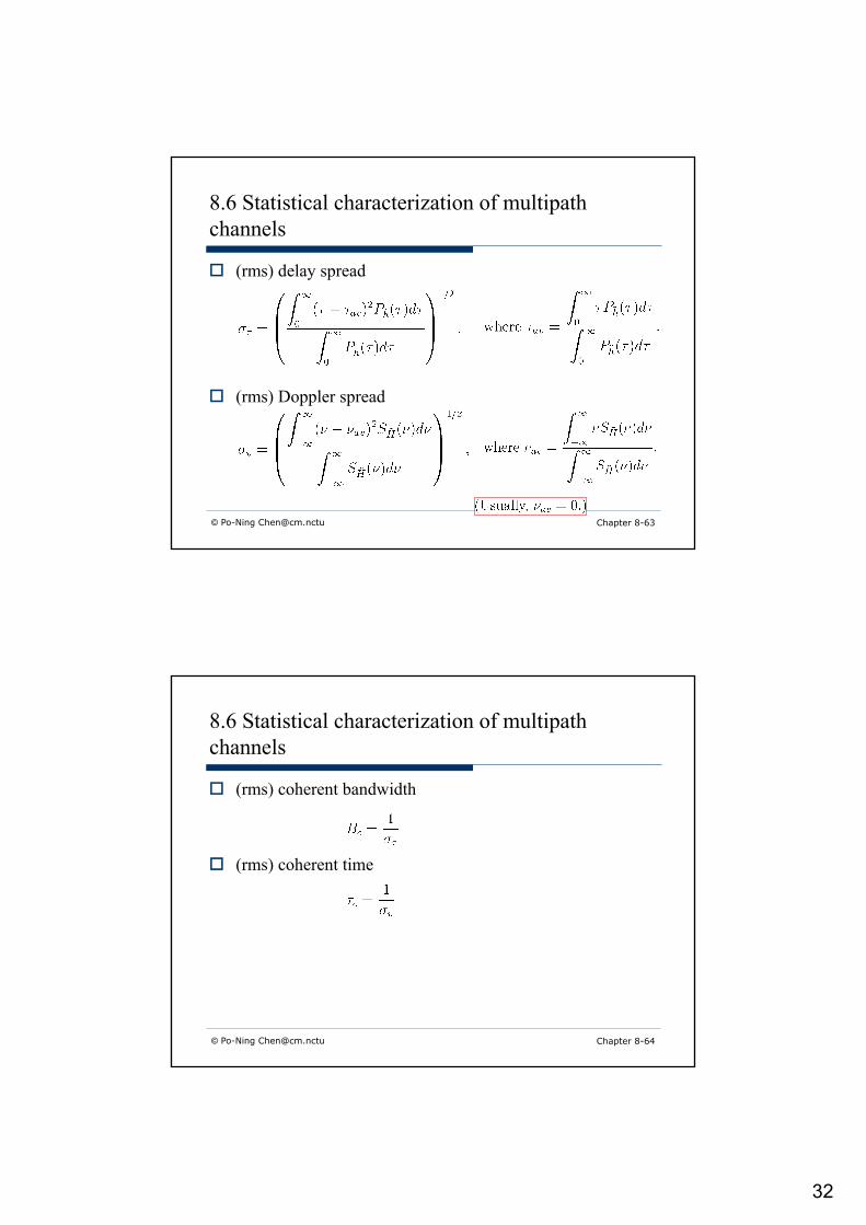
8.6 Statistical characterization of multipath channels
o (rms) delay spread
o (rms) Doppler spread
© Po-Ning [email protected] Chapter 8-64
8.6 Statistical characterization of multipath channels
o (rms) coherent bandwidth
o (rms) coherent time
33
© Po-Ning [email protected] Chapter 8-65
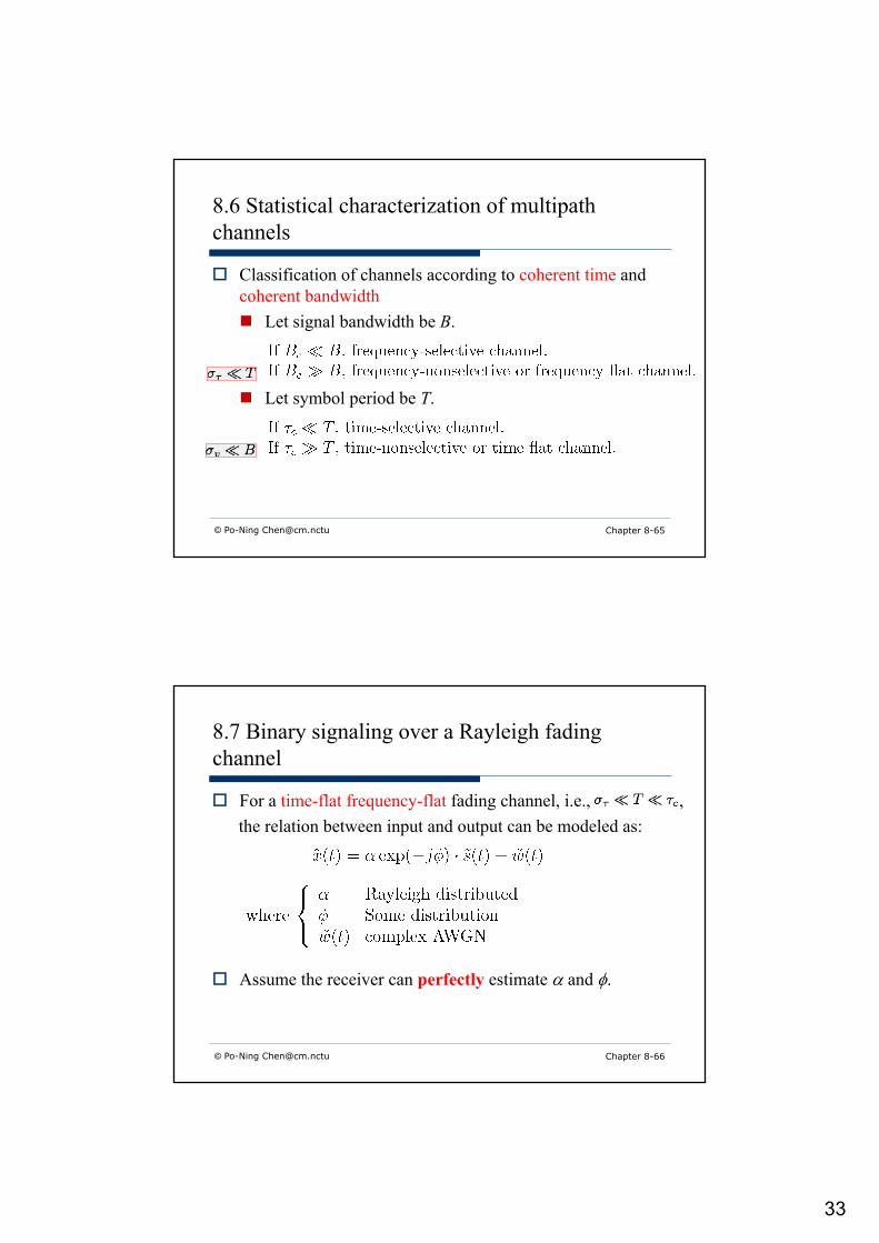
8.6 Statistical characterization of multipath channels
o Classification of channels according to coherent time and coherent bandwidthn Let signal bandwidth be B.
n Let symbol period be T.
© Po-Ning [email protected] Chapter 8-66
8.7 Binary signaling over a Rayleigh fading channel
o For a time-flat frequency-flat fading channel, i.e., ,the relation between input and output can be modeled as:
o Assume the receiver can perfectly estimate a and f.
34
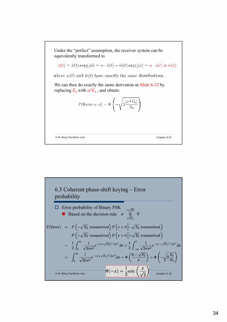
© Po-Ning [email protected] Chapter 8-67
Under the “perfect” assumption, the receiver system can be equivalently transformed to
We can then do exactly the same derivation as Slide 6-32 by replacing Eb with a2Eb , and obtain:
6.3 Coherent phase-shift keying – Error probability
o Error probability of Binary PSKn Based on the decision rule
© Po-Ning [email protected] Chapter 6-32
36
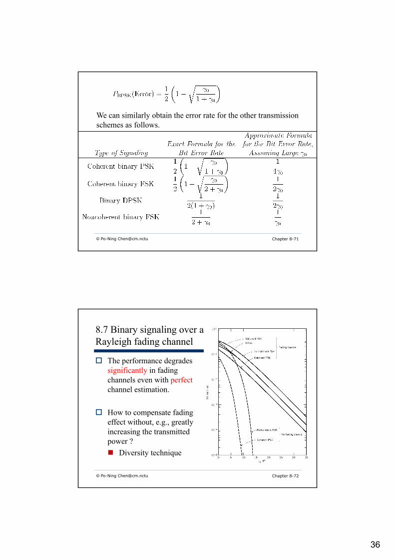
© Po-Ning [email protected] Chapter 8-71
We can similarly obtain the error rate for the other transmission schemes as follows.
© Po-Ning [email protected] Chapter 8-72
8.7 Binary signaling over a Rayleigh fading channel
o The performance degrades significantly in fading channels even with perfectchannel estimation.
o How to compensate fading effect without, e.g., greatly increasing the transmitted power ?n Diversity technique
37
© Po-Ning [email protected] Chapter 8-73
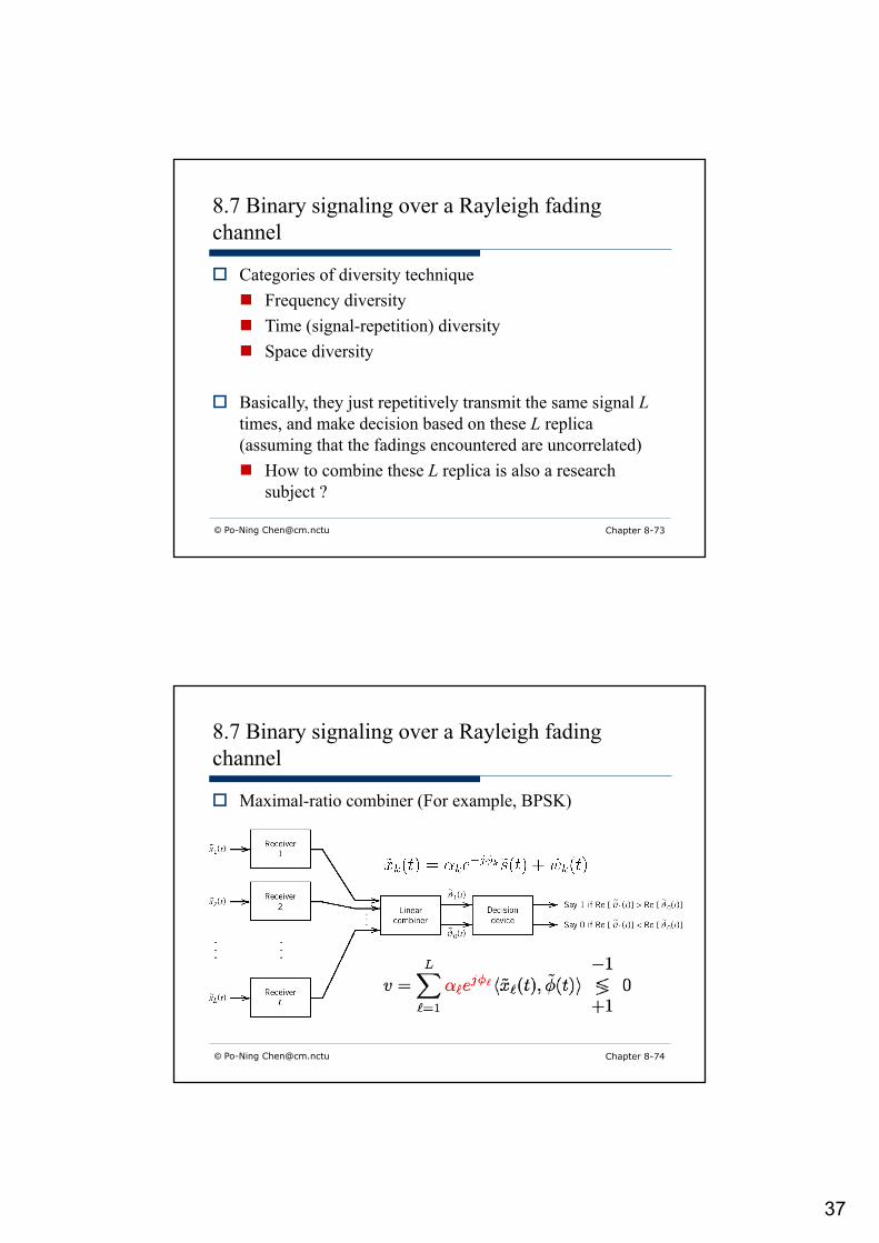
8.7 Binary signaling over a Rayleigh fading channel
o Categories of diversity techniquen Frequency diversityn Time (signal-repetition) diversityn Space diversity
o Basically, they just repetitively transmit the same signal Ltimes, and make decision based on these L replica (assuming that the fadings encountered are uncorrelated)n How to combine these L replica is also a research
subject ?
© Po-Ning [email protected] Chapter 8-74
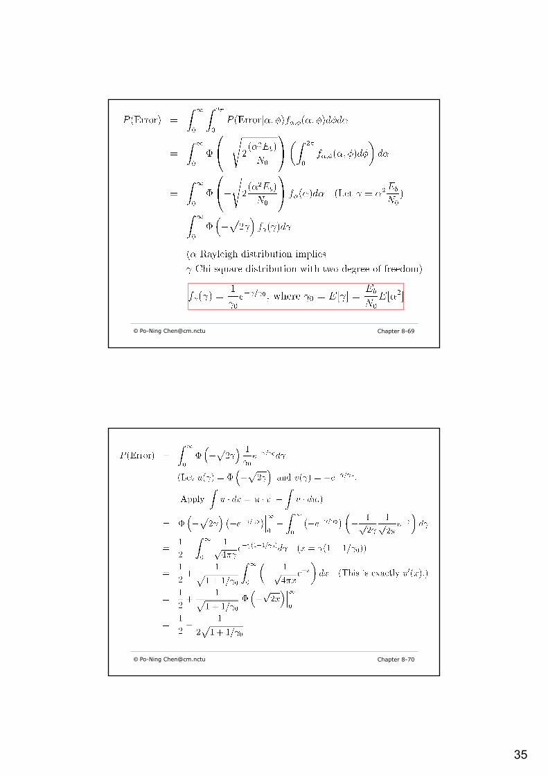
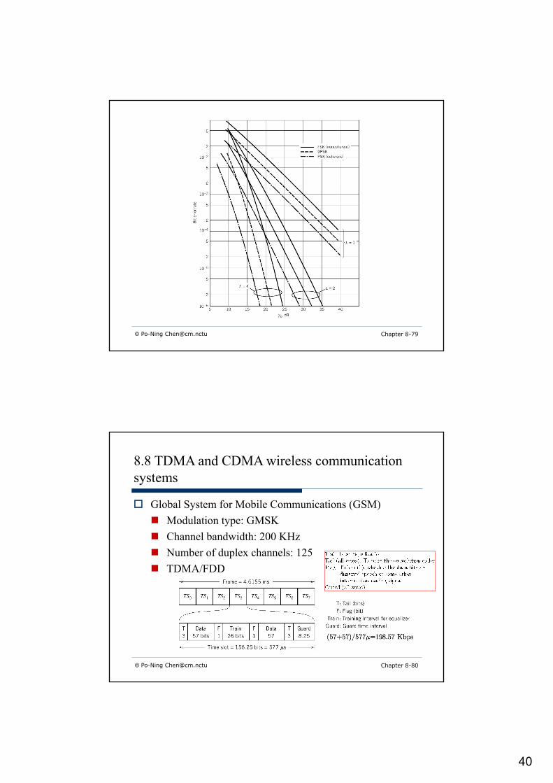
8.7 Binary signaling over a Rayleigh fading channel
o Maximal-ratio combiner (For example, BPSK)
39
© Po-Ning [email protected] Chapter 8-77
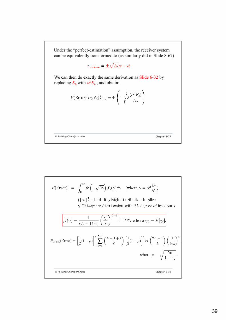
Under the “perfect-estimation” assumption, the receiver system can be equivalently transformed to (as similarly did in Slide 8-67)
We can then do exactly the same derivation as Slide 6-32 by replacing Eb with a2Eb , and obtain:
© Po-Ning [email protected] Chapter 8-78
40
© Po-Ning [email protected] Chapter 8-79
© Po-Ning [email protected] Chapter 8-80
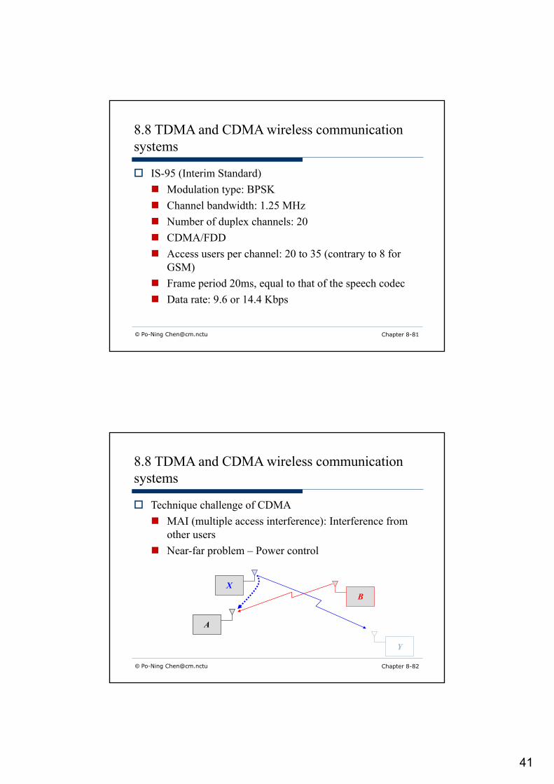
8.8 TDMA and CDMA wireless communication systems
o Global System for Mobile Communications (GSM)n Modulation type: GMSKn Channel bandwidth: 200 KHzn Number of duplex channels: 125n TDMA/FDD
41
© Po-Ning [email protected] Chapter 8-81
8.8 TDMA and CDMA wireless communication systems
o IS-95 (Interim Standard)n Modulation type: BPSKn Channel bandwidth: 1.25 MHzn Number of duplex channels: 20n CDMA/FDDn Access users per channel: 20 to 35 (contrary to 8 for
GSM)n Frame period 20ms, equal to that of the speech codecn Data rate: 9.6 or 14.4 Kbps
© Po-Ning [email protected] Chapter 8-82
8.8 TDMA and CDMA wireless communication systems
o Technique challenge of CDMAn MAI (multiple access interference): Interference from
other usersn Near-far problem – Power control
X
A
Y
B
42
© Po-Ning [email protected] Chapter 8-83
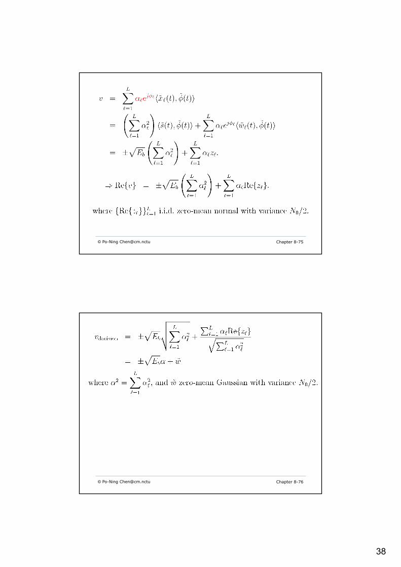
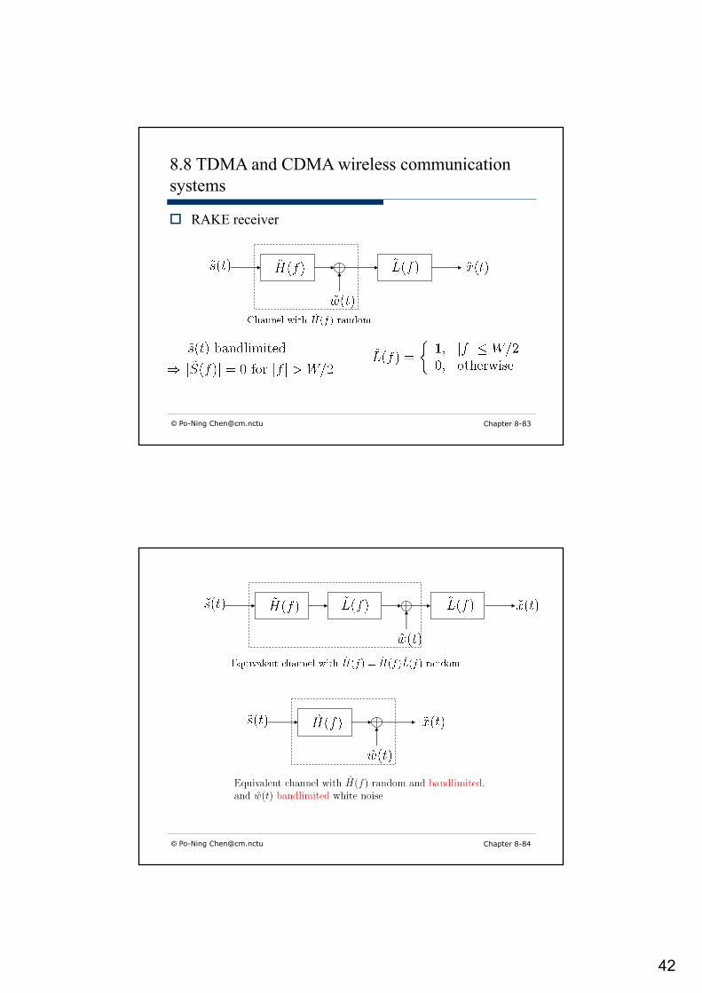
8.8 TDMA and CDMA wireless communication systems
o RAKE receiver
© Po-Ning [email protected] Chapter 8-84
44
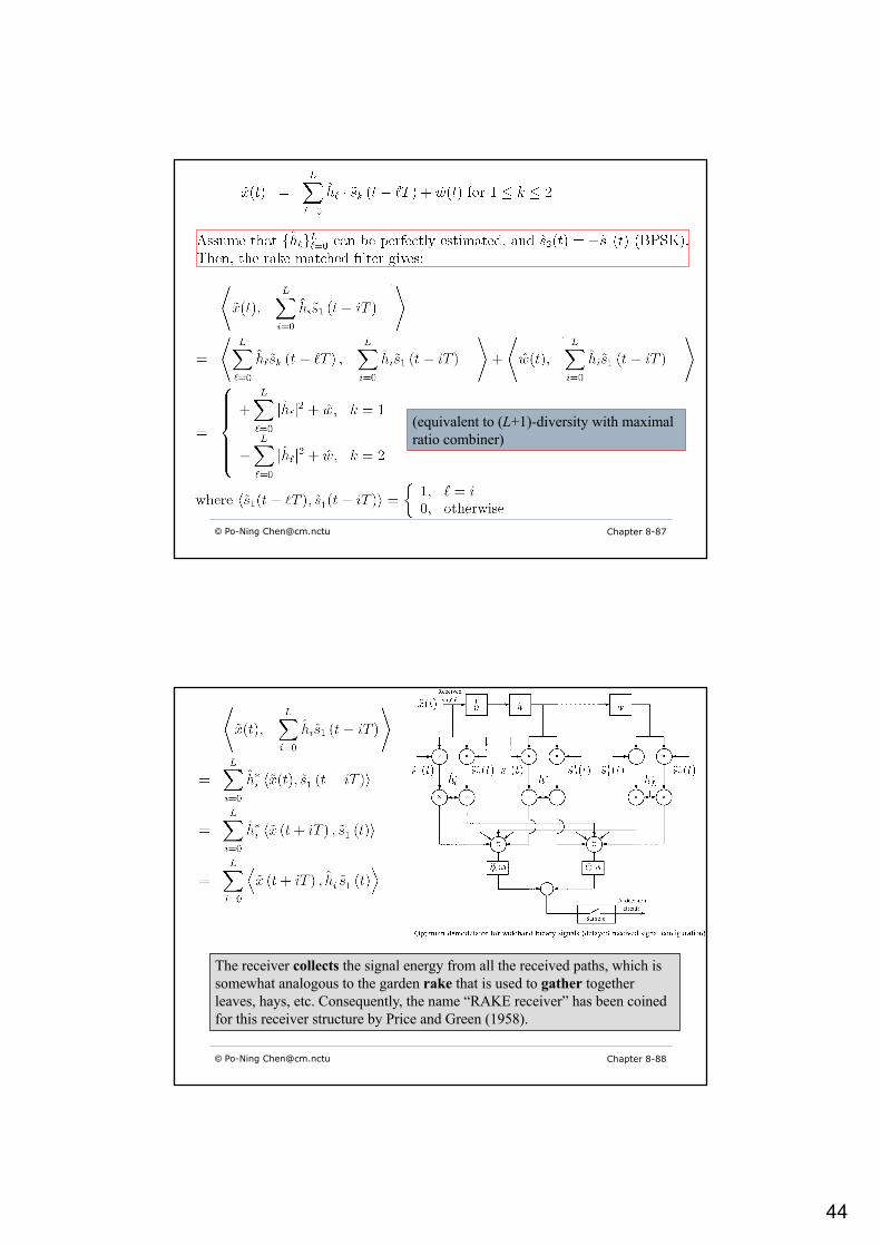
© Po-Ning [email protected] Chapter 8-87
(equivalent to (L+1)-diversity with maximal ratio combiner)
© Po-Ning [email protected] Chapter 8-88
The receiver collects the signal energy from all the received paths, which is somewhat analogous to the garden rake that is used to gather together leaves, hays, etc. Consequently, the name “RAKE receiver” has been coined for this receiver structure by Price and Green (1958).
45
© Po-Ning [email protected] Chapter 8-89
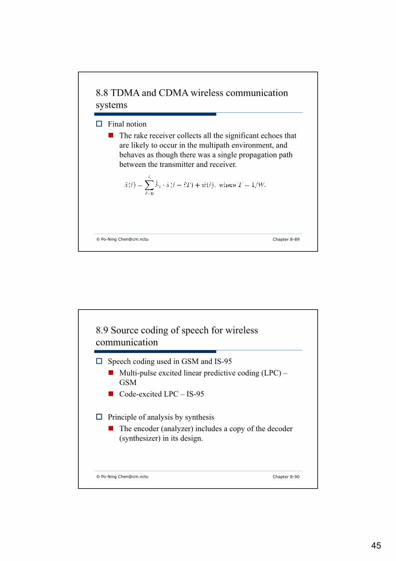
8.8 TDMA and CDMA wireless communication systems
o Final notionn The rake receiver collects all the significant echoes that
are likely to occur in the multipath environment, and behaves as though there was a single propagation path between the transmitter and receiver.
© Po-Ning [email protected] Chapter 8-90
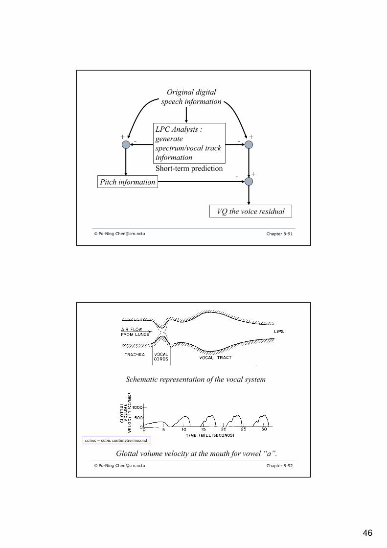
8.9 Source coding of speech for wireless communication
o Speech coding used in GSM and IS-95n Multi-pulse excited linear predictive coding (LPC) –
GSMn Code-excited LPC – IS-95
o Principle of analysis by synthesisn The encoder (analyzer) includes a copy of the decoder
(synthesizer) in its design.
46
Original digitalspeech information
+ +
+
- -
-
LPC Analysis : generatespectrum/vocal trackinformation
Pitch information
VQ the voice residual
Short-term prediction
© Po-Ning [email protected] Chapter 8-91
© Po-Ning [email protected] Chapter 8-92
Schematic representation of the vocal system
Glottal volume velocity at the mouth for vowel “a”.
cc/sec = cubic centimetres/second
47
© Po-Ning [email protected] Chapter 8-93
D
D
a1
a9
a10
+
excitation speech
+
+
+
å=
--== 10
11
1)(
1)()(
j
jj za
zAzGzX
å=
--=10
1
][][][j
j jnxanxng
LipsVocal tractGlottal volume
x[n]g[n]
Synthesis filter (analysis by synthesis)
© Po-Ning [email protected] Chapter 8-94
Encoder Decoder
Multi-pulse excited linear predictive codec
48
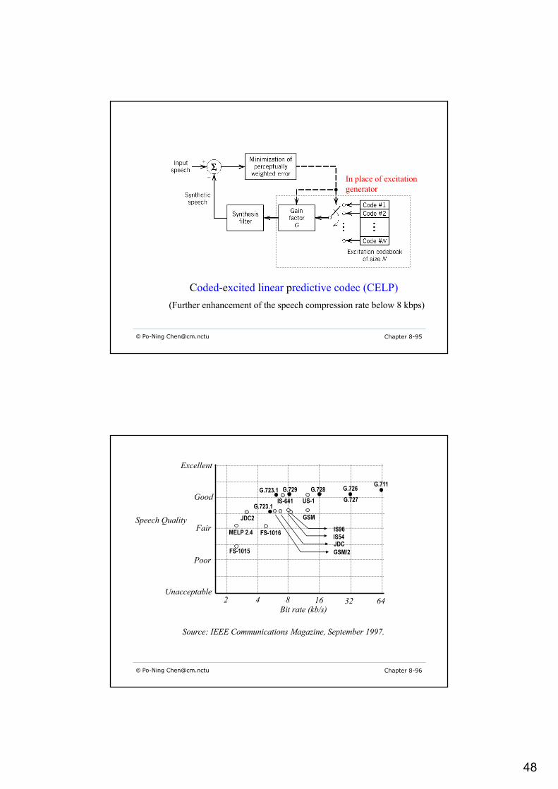
© Po-Ning [email protected] Chapter 8-95
Coded-excited linear predictive codec (CELP)
In place of excitation generator
(Further enhancement of the speech compression rate below 8 kbps)
© Po-Ning [email protected] Chapter 8-96
2 4 8 16 32 64Unacceptable
Poor
Fair
Good
Excellent
Bit rate (kb/s)
Speech Quality
FS-1015
MELP 2.4 FS-1016
JDC2
G.723.1
GSM/2JDCIS54IS96
GSM
G.723.1 G.729 G.728 G.726 G.711
G.727IS-641 US-1
Source: IEEE Communications Magazine, September 1997.
49
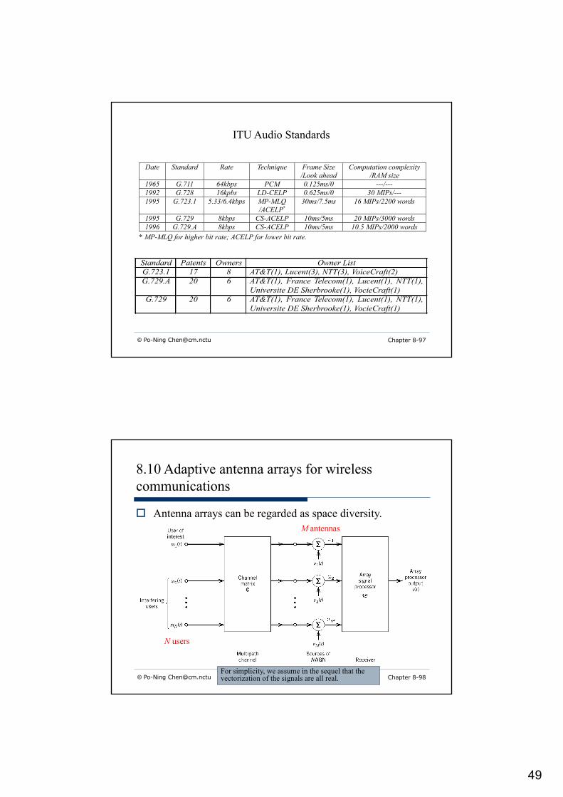
© Po-Ning [email protected] Chapter 8-97
Date Standard Rate Technique Frame Size/Look ahead
Computation complexity/RAM size
1965 G.711 64kbps PCM 0.125ms/0 ---/---1992 G.728 16kpbs LD-CELP 0.625ms/0 30 MIPs/---1995 G.723.1 5.33/6.4kbps MP-MLQ
/ACELP*30ms/7.5ms 16 MIPs/2200 words
1995 G.729 8kbps CS-ACELP 10ms/5ms 20 MIPs/3000 words1996 G.729.A 8kbps CS-ACELP 10ms/5ms 10.5 MIPs/2000 words
* MP-MLQ for higher bit rate; ACELP for lower bit rate.
Standard Patents Owners Owner List G.723.1 17 8 AT&T(1), Lucent(3), NTT(3), VoiceCraft(2) G.729.A 20 6 AT&T(1), France Telecom(1), Lucent(1), NTT(1),
Universite DE Sherbrooke(1), VocieCraft(1) G.729 20 6 AT&T(1), France Telecom(1), Lucent(1), NTT(1),
Universite DE Sherbrooke(1), VocieCraft(1)
ITU Audio Standards
© Po-Ning [email protected] Chapter 8-98
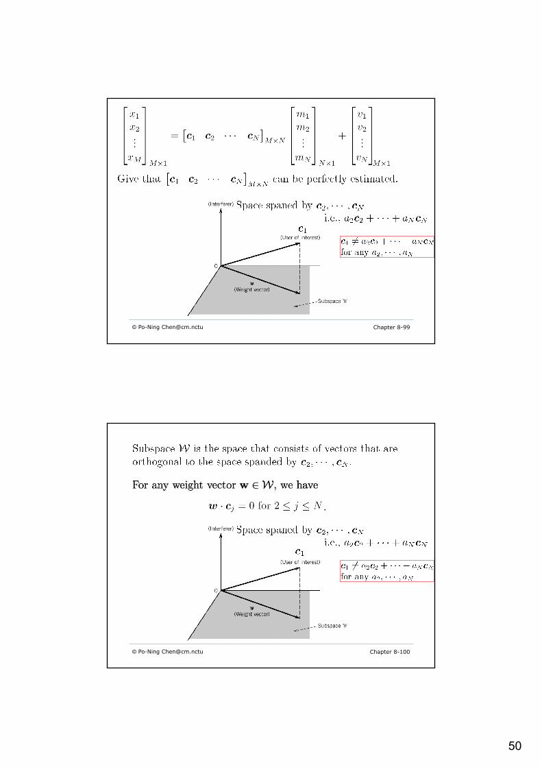
8.10 Adaptive antenna arrays for wireless communications
o Antenna arrays can be regarded as space diversity.M antennas
N users
For simplicity, we assume in the sequel that the vectorization of the signals are all real.
51
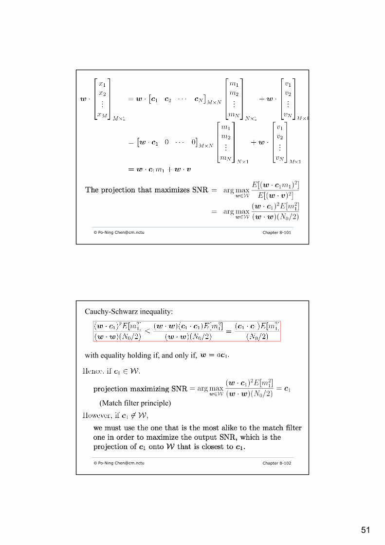
© Po-Ning [email protected] Chapter 8-101
© Po-Ning [email protected] Chapter 8-102
with equality holding if, and only if,
(Match filter principle)
Cauchy-Schwarz inequality:
52
© Po-Ning [email protected] Chapter 8-103
Example. What is the dimension of W, if
Answer:?
© Po-Ning [email protected] Chapter 8-104
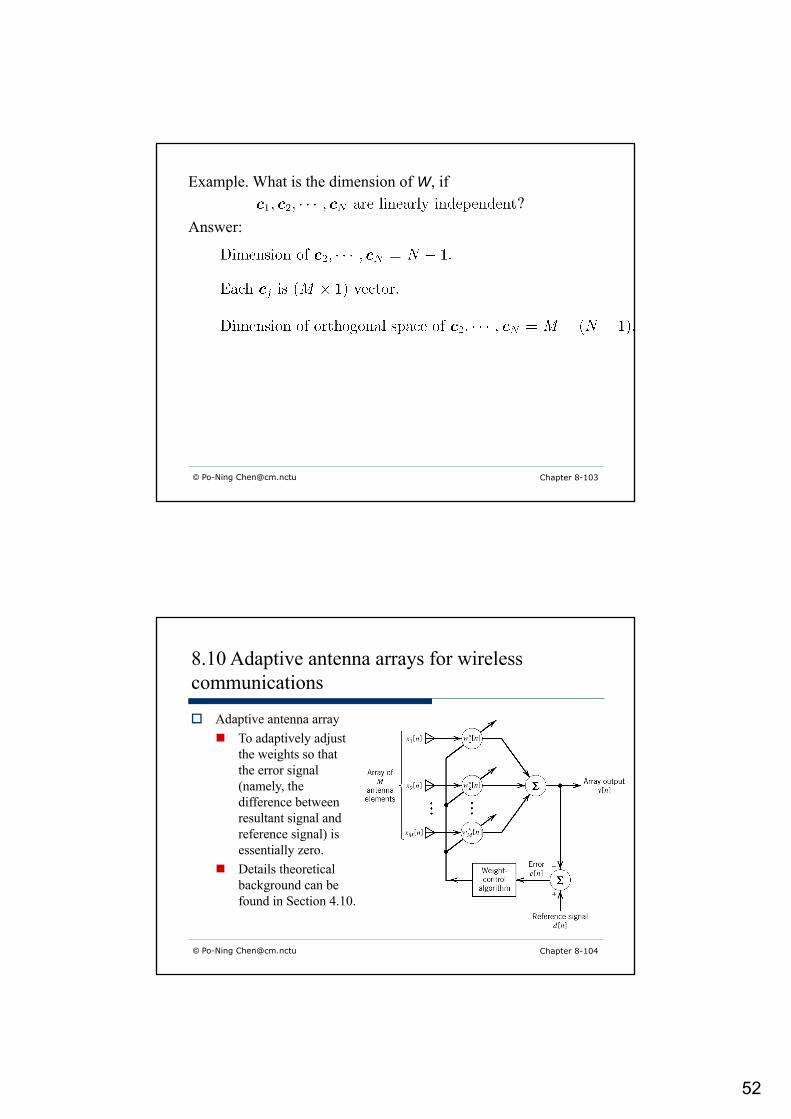
8.10 Adaptive antenna arrays for wireless communications
o Adaptive antenna arrayn To adaptively adjust
the weights so that the error signal (namely, the difference between resultant signal and reference signal) is essentially zero.
n Details theoretical background can be found in Section 4.10.
Recommended