Download pdf - Chapter 10 Introducing Python Pandas · = pandas.Series(data=None , index=None , dtype=None) None is the default value for different parameters taken in case

P a g e 1 | 57

Chapter 10 – Introducing Python Pandas

Introduction

Python Panda is Python’s library for data analysis.

Panda – “ Panel Data Analysis”

What is Data Analysis?

It refers to process of evaluating big data sets using analytical & statistical tools so as to discover useful information and

conclusion to support business decision making.

Python pandas & Data Analysis

Python pandas provide various tools for data analysis and makes it a simple and easy process.

Author of Pandas is Wes Mckinney.

Using Pandas

Pandas is an opens source library built for Python programming language, which provides high performance

data analysis tools.

In order to work with pandas in Python, you need to import pandas library in your python environment.

Benefits of using Panda for Data Analysis

1. It can read or write in many different data formats(integer,float,double,etc.)

2. It can calculate in all ways data is organized, i.e., across rows and down columns.

3. It can easily select subsets of data from bulky data sets and even combine multiple datasets together.

4. It has functionality to find and fill missing data.

5. It supports advanced time-series functionality(Time series forecasting is the use of a model to predict future

values based on previously observed values)

**Pandas is best at handling huge tabular data sets comprising different data formats.

NumPy Arrays

NumPy(‘Numerical Python’ or ‘Numeric Python’) is an open source module of Python that offers functions and

routines for fast mathematical computation on array and matrices.

In order to use Numpy, you must import in your module by using a statement like:

import numpy as np

The above statement has given np as alias name for numpy module. Once imported you can use

both names i.e. numpy or np for functions, e.g. numpy.array( ) is same as np.array( ).

Array

It refers to a named group of homogenous (of same type) elements. E.g. students array containing 5

entries as [34, 37, 36, 41, 40] then students is an array.

Types of Numpy array

A NumPy array is simply a grid that contains values of the same/homogenous type. NumPy Arrays

come in two forms:

1-D(one dimensional) arrays known as Vectors(having single row/column only)

Multidimensional arrays known as Matrices(can have multiple rows and columns)

You can use any identifier name in place of

np

P a g e 2 | 57

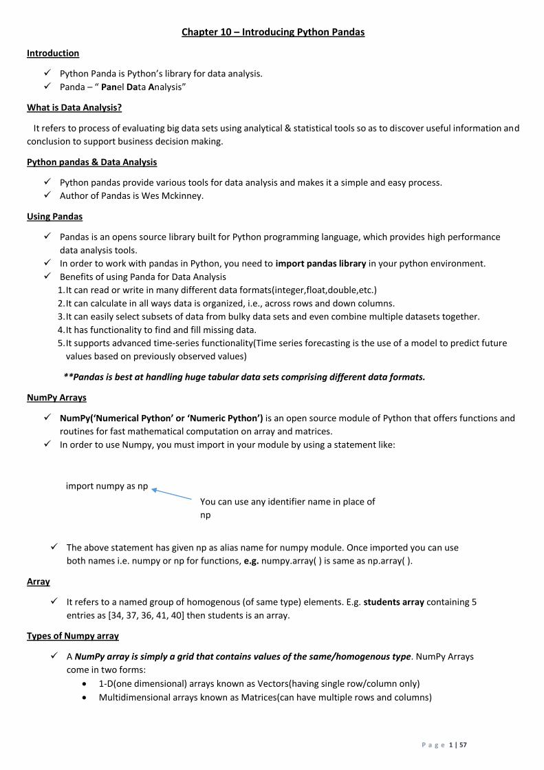
Example 1: (1-D array)

import numpy as np

list = [1,2,3,4]

a1=np.array(list)

print(a1)

Output : [1 , 2 , 3 , 4]

**Individual elements of above array can be accessed just like you access a list’s i.e. arrayname [index]

Example 2: (2-D array)

import numpy as np

a7 = np.array([ [10,11,12,13] , [21,22,23,24] ])

print(a7[1,3])

print(a7[1][3])

print(a7)

Output:

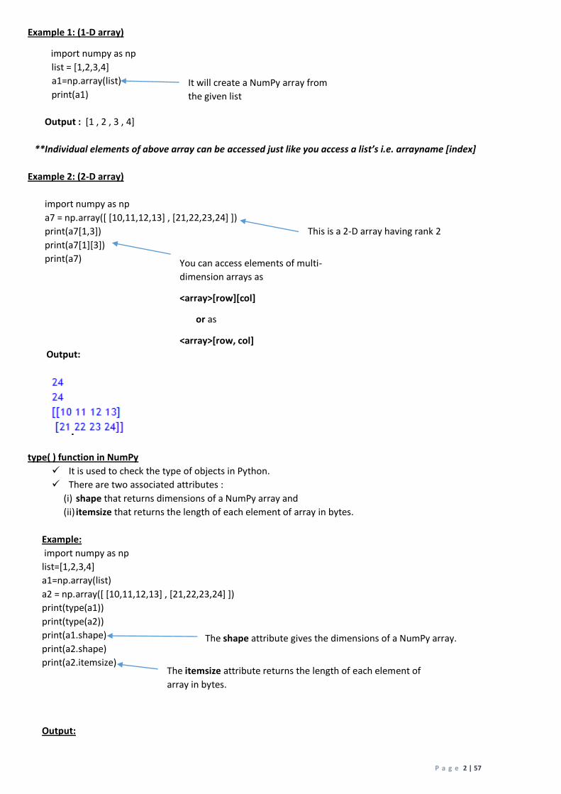
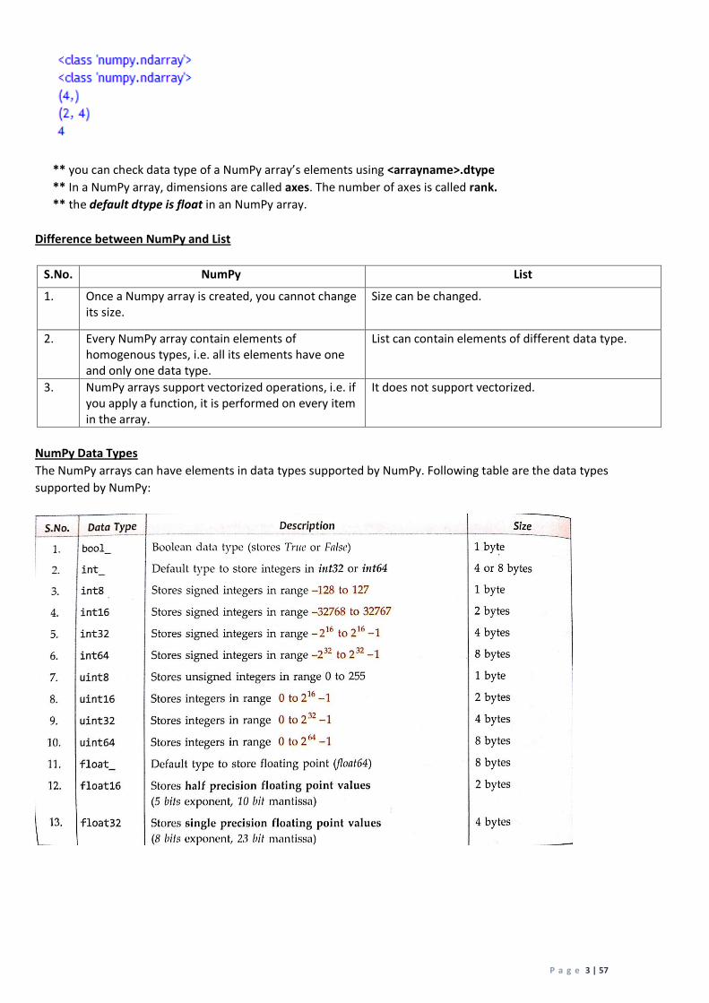
type( ) function in NumPy

It is used to check the type of objects in Python.

There are two associated attributes :

(i) shape that returns dimensions of a NumPy array and

(ii) itemsize that returns the length of each element of array in bytes.

Example:

import numpy as np

list=[1,2,3,4]

a1=np.array(list)

a2 = np.array([ [10,11,12,13] , [21,22,23,24] ])

print(type(a1))

print(type(a2))

print(a1.shape)

print(a2.shape)

print(a2.itemsize)

Output:

It will create a NumPy array from

the given list

This is a 2-D array having rank 2

You can access elements of multi-

dimension arrays as

<array>[row][col]

or as

<array>[row, col]

The shape attribute gives the dimensions of a NumPy array.

The itemsize attribute returns the length of each element of

array in bytes.

P a g e 3 | 57

** you can check data type of a NumPy array’s elements using <arrayname>.dtype

** In a NumPy array, dimensions are called axes. The number of axes is called rank.

** the default dtype is float in an NumPy array.

Difference between NumPy and List

S.No. NumPy List

1. Once a Numpy array is created, you cannot change its size.

Size can be changed.

2. Every NumPy array contain elements of homogenous types, i.e. all its elements have one and only one data type.

List can contain elements of different data type.

3. NumPy arrays support vectorized operations, i.e. if you apply a function, it is performed on every item in the array.

It does not support vectorized.

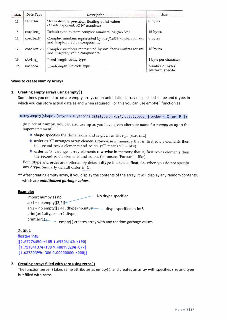
NumPy Data Types

The NumPy arrays can have elements in data types supported by NumPy. Following table are the data types

supported by NumPy:

P a g e 4 | 57

Ways to create NumPy Arrays

1. Creating empty arrays using empty( )

Sometimes you need to create empty arrays or an uninitialized array of specified shape and dtype, in

which you can store actual data as and when required. For this you can use empty( ) function as:

** After creating empty array, if you display the contents of the array, it will display any random contents,

which are uninitialized garbage values.

Example:

import numpy as np

arr1 = np.empty([3,2])

arr2 = np.empty([3,4] , dtype=np.int8)

print(arr1.dtype , arr2.dtype)

print(arr1)

Output:

2. Creating arrays filled with zero using zeros( )

The function zeros( ) takes same attributes as empty( ), and creates an array with specifies size and type

but filled with zeros.

No dtype specified

dtype specified as int8

empty( ) creates array with any random garbage values

P a g e 5 | 57

Example:

import numpy as np

arr1 = np.zeros([3,2],dtype=np.int64)

print(arr1)

Output:

3. Creating arrays filled with 1’s using ones( )

The function ones( ) takes same attributes as empty( ), and creates an array with specified size and type

but filled with ones.

Example:

import numpy as np

arr1 = np.ones([3,2],dtype=np.int64)

print(arr1)

Output:

** There are three more functions empty_like( ), zeros_like( ) and ones_like( ) that you can use to create an

array similar to another existing array.

4. Creating arrays with a numerical range using arange( )

arange( ) creates a NumPy array with evenly spaced values within a specified numerical range. It is used

as:

Example:

import numpy as np

P a g e 6 | 57

arr1 = np.arange(7)

print(arr1)

arr2=np.arange(1,7,2,np.float32)

print(arr2)

Output:

5. Creating arrays with a numerical range using linspace( )

linspace( ) is used to generate evenly spaced elements between two given limits.

Example:

import numpy as np

arr1 = np.linspace(2,10,3)

print(arr1)

Output:

Pandas Data Structure

A data structure is a particular way of storing and organizing data in a computer to suit a specific purpose so that

it can be accessed and worked with in appropriate ways.

Two basic data structure in Pandas are : Series and Dataframe

Series Data Structure

It represents a one-dimensional array of indexed data. A series type object has two main components:

1. An array of actual data

2. An associated array of indexes or data labels.

Creating Series Objects

A series type object/variable can be created using panda library series( ). Make sure that you have imported pandas

and numpy modules with import statements.

I. Creating empty series Object

To create an empty object i.e., having no values, you can just use the series( ) as :

<series object> = pandas.Series( )

The above statement will create an empty series type object with no value having default datatype which is

float64.

Example:

import numpy as np

P a g e 7 | 57

import pandas as pd

obj1 = pd.Series( )

print(obj1)

Output: Series([], dtype: float64)

II. Creating non-empty Series objects

To create non-empty Series objects, you need to specify arguments for data and indexes as per following syntax:

<Series-object> = pd.Series(data , index=idx)

where data is the data part of the Series object, it can be one of the following:

* A Python sequence * An ndarray * A Python dictionary * A Scalar Value

(i) Specify data as Python Sequence

<Series-object> = pd.Series(<any Python sequence>)

Example:

import numpy as np

import pandas as pd

obj1 = pd.Series(range(7))

obj2 = pd.Series([3.5 , 5 ,6.5, 8])

print(obj1)

print(obj2)

Output:

(ii) Specify data as ndarray

The data attribute can be ndarray also.

Example:

import numpy as np

import pandas as pd

arr1=np.array([2,4,6,8])

obj1 = pd.Series(arr1)

print(obj1)

Output:

P a g e 8 | 57

(iii) Specify data as a Python dictionary

The sequence that you provide with Series( ) can be any sequence, including dictionaries.

Example:

import numpy as np

import pandas as pd

obj1 = pd.Series({'Jan': 31 , 'Feb' : 28 , 'Mar' : 31})

print(obj1)

Output:

(iv) Specify data as a scalar value

The data can be in form of a single value or a scalar value. BUT if data is scalar value, then the index must be

provided. The scalar value(given as data) will be repeated to match the length of index. E.g.

III. Creating Series Objects – Additional Functionality

(i) Specifying/Adding Nan Values in a Series object

Sometimes you need to create a series object of a certain size but you do not have complete data available at that

time. In such cases, you can fill missing data with a NaN(Not a Number) value.

Example:

import numpy as np

import pandas as pd

obj1 = pd.Series([2.4 , np.NaN , 3.8])

print(obj1)

P a g e 9 | 57

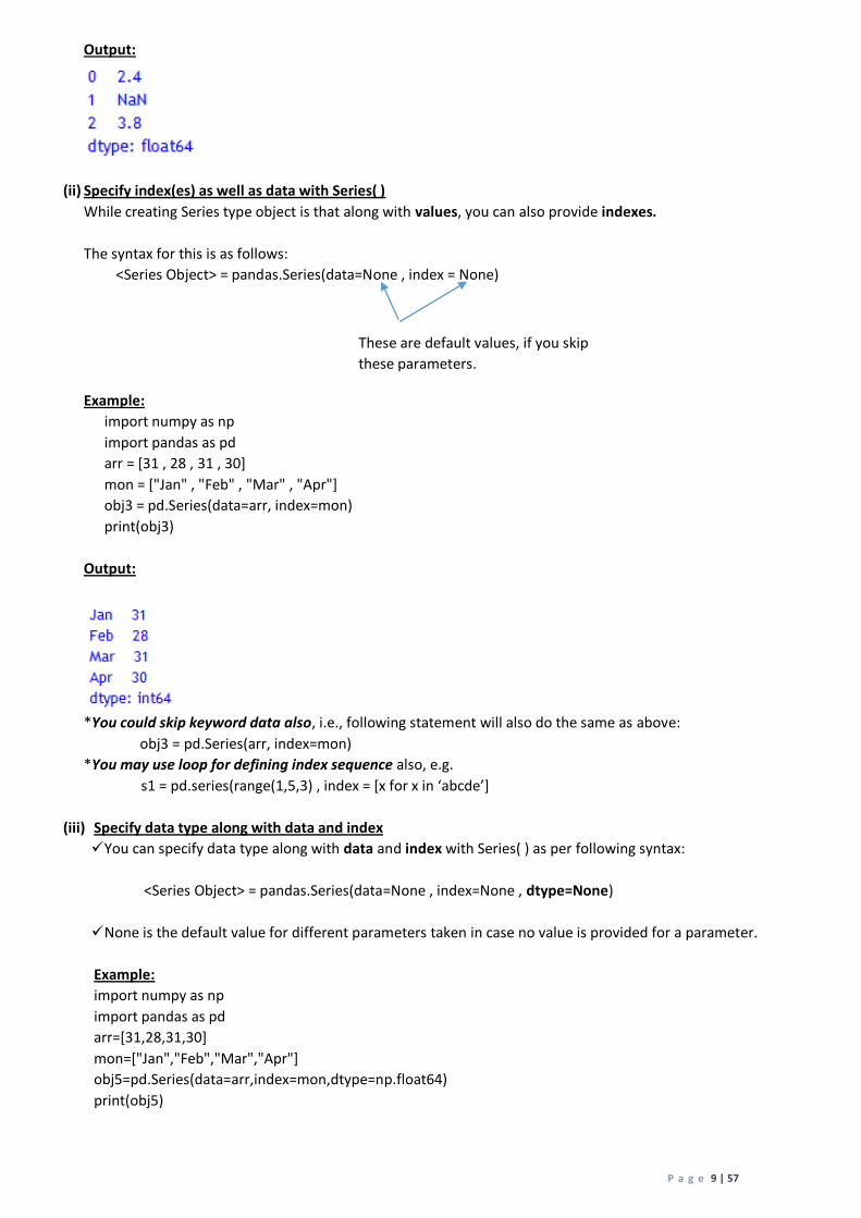
Output:

(ii) Specify index(es) as well as data with Series( )

While creating Series type object is that along with values, you can also provide indexes.

The syntax for this is as follows:

<Series Object> = pandas.Series(data=None , index = None)

Example:

import numpy as np

import pandas as pd

arr = [31 , 28 , 31 , 30]

mon = ["Jan" , "Feb" , "Mar" , "Apr"]

obj3 = pd.Series(data=arr, index=mon)

print(obj3)

Output:

*You could skip keyword data also, i.e., following statement will also do the same as above:

obj3 = pd.Series(arr, index=mon)

*You may use loop for defining index sequence also, e.g.

s1 = pd.series(range(1,5,3) , index = [x for x in ‘abcde’]

(iii) Specify data type along with data and index

You can specify data type along with data and index with Series( ) as per following syntax:

<Series Object> = pandas.Series(data=None , index=None , dtype=None)

None is the default value for different parameters taken in case no value is provided for a parameter.

Example:

import numpy as np

import pandas as pd

arr=[31,28,31,30]

mon=["Jan","Feb","Mar","Apr"]

obj5=pd.Series(data=arr,index=mon,dtype=np.float64)

print(obj5)

These are default values, if you skip

these parameters.

P a g e 10 | 57

Output:

(iv) Using a mathematical function/expression to create data array in Series( )

The Series( ) allows you to define a function or expression that can calculate values for data sequence. It is

done in following form:

<Series Object> = pandas.Series(index=None, data=<function|expression>)

Example1:

import numpy as np

import pandas as pd

a= np.arange(9,13)

print(a)

obj1 = pd.Series(index=a, data=a*2)

print(obj1)

obj2 = pd.Series(index=a, data= a**2)

print(obj2)

Output:

Example2:

import numpy as np

import pandas as pd

list1=[10,20,30,40]

obj1 = pd.Series(data=list1*2)

print(obj1)

Output:

P a g e 11 | 57

** A number multiplied with a list replicates the list those many times and hence the data array has the same

list values replicated twice. ( 2 * list1)

Important

While creating a Series object, when you give index array as a sequence then there is no compulsion for the uniqueness

of indexes. That is, you have duplicate entries in the index array and Python won’t raise any error.

e.g.

import numpy as np

import pandas as pd

val=np.array([10,20,30,40])

obj1 = pd.Series(index=['a','b','a','b'],data=val)

print(obj1)

Output:

Series Object Attributes

When you create a Series type object, all information related to it(such as its size, its datatype etc.) is available

through attributes. You can use these attributes in the following format to get information about the Series

object:

<Series object>.<attribute name>

(a) Retrieving Index Array and Data Array of a Series Object

See, index array has duplicate entries.

P a g e 12 | 57

You can access the index array and data values array of an existing Series object by using attributes index and

values.

Example:

import numpy as np

import pandas as pd

obj5=pd.Series(data=[10,20,30,40])

obj6=pd.Series(data=[56.6,70.5,78.6], index=['a','b','c'])

print(obj5.index)

print(obj5.values)

print(obj6.index)

print(obj6.values)

Output:

(b) Retrieving Types(dtype) and Size of Type(itemsize)

To retrieve the data type of individual elements of a series object, you can use attribute dtype with Series object as

<objectname>.dtype . You can use itemsize attribute to know the number of bytes allocated to each data item,

e.g.

import numpy as np

import pandas as pd


obj6=pd.Series(data=[56.6,70.5,78.6], index=['a','b','c'])

print(obj5.dtype)

print(obj5.itemsize)

print(obj6.dtype)

print(obj6.itemsize)

Output:

int64

8

float64

8

(c) Retrieving Shape

The shape of a Series object tells how big it is, i.e., how many elements it contains including missing or empty

values(NaN). Since there is only one axis in Series object, it is shown as (<n>, ), where n is the number of elements in

the object.

e.g.

import numpy as np

import pandas as pd


obj6=pd.Series(data=[56.6,70.5,78.6],index=['a','b','c'])

print(obj5.shape)

print(obj6.shape)

Output:

P a g e 13 | 57

(d) Retrieving Dimension, Size and Number of Bytes

e.g.

import numpy as np

import pandas as pd



print(obj5.ndim, obj6.ndim)

print(obj5.size, obj6.size)

print(obj5.nbytes, obj6.nbytes)

Output:

(e) Checking Emptiness and Presence of NaNs

If you want to check if the Series object is empty, then you can do it by checking the empty attribute as shown

below. Similarly if you want to check if a Series object contains some NaN value or not, you can use hasnans

attribute.

If you use len( ) on a series object, then it returns total elements in it including NaNs but <series>.count() returns

only the count of non-NaN values in a Series object.

e.g.

import numpy as np

import pandas as pd

obj5=pd.Series(data=[10,20,30,np.NaN])


obj7=pd.Series()

print(obj5.empty, obj6.empty, obj7.empty)

print(obj5.hasnans,obj6.hasnans,obj7.hasnans)

print(len(obj5),len(obj6))

print(obj5.count( ),obj6.count( ))

Output:

Accessing a Series Object and it Elements

After creating Series type object,you can access its indexes separately, its data separately and even access

individual elements.

P a g e 14 | 57

1. Accessing Individual Elements

To access individual elements of a Series object, you can give its index in square bracket along with its name as you

have been doing with other Python sequence, i.e., as :

<Series Object name> [<valid index>]

Example:

import numpy as np

import pandas as pd


obj6=pd.Series(data=[56.6,70.5,78.6,89.8],index=['a','b','c','a'])

print(obj5[2], obj5[3])

print(obj6['b'], obj6['c'])

print(obj6['a'])

Output:

** Only legal and valid indexes should be used inside the square bracket.

** If the series object has duplicate indexes, then giving an index with the Series object will return all the entries

with that index.

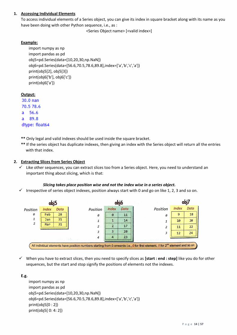
2. Extracting Slices from Series Object

Like other sequences, you can extract slices too from a Series object. Here, you need to understand an

important thing about slicing, which is that:

Slicing takes place position wise and not the index wise in a series object.

Irrespective of series object indexes, position always start with 0 and go on like 1, 2, 3 and so on.

When you have to extract slices, then you need to specify slices as [start : end : step] like you do for other

sequences, but the start and stop signify the positions of elements not the indexes.

E.g.

import numpy as np

import pandas as pd



print(obj5[0 : 2])

print(obj5[ 0: 4: 2])

P a g e 15 | 57

print(obj5[: :-1])

print(obj6[0 : : 2])

print(obj6[ 4: 5])

Output:

Operations on Series Object

1. Modifying Elements of Series Object

The data values of a Series object can be easily modified through item assignment, i.e.

<SeriesObject> [<index>] = <new_data_value>

Above assignment will change the data value of the given index in Series Object.

<SeriesObject>[start : stop] = <new_data_value>

Above assignment will replace all the values falling in given slice.

You can even change indexes of a Series object by assigning new index array to its index attribute, i.e.

<Object>.index = <new index array>

But the size of new index array must match with existing index array’s size.

Example:

import numpy as np

import pandas as pd



obj5[0]=20

obj6['b']=67.8

print(obj5)

print(obj6)

obj6.index = ['x','y','z','x']

print(obj6)

Output:

P a g e 16 | 57

2. The head( ) and tail( ) functions

The head( ) function is used to fetch first n rows from a pandas object and tail( ) function returns last n rows

from a pandas object. The syntax to use these functions is :

<pandas object>.head([n])

Or <pandas object>.tail([n])

If you do not provide any value for n, then head( ) and tail( ) will return first 5 and last 5 rows respectively of

pandas object.

Example:

import numpy as np

import pandas as pd



print(obj5.head( ))

print(obj6.tail( ))

print(obj5.head(2))

print(obj6.tail(3))

Output:

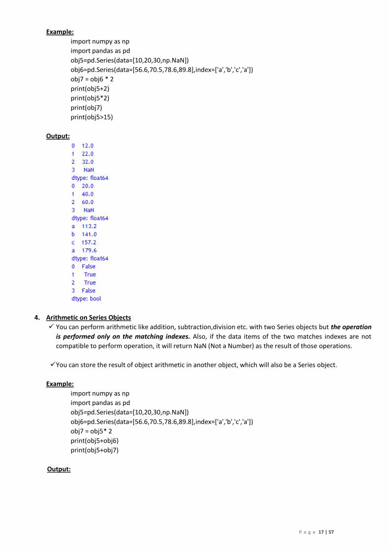
3. Vector operations on Series Object

Vector operations mean that if you apply a function or expression then it is individually applied on each

item of the object.

P a g e 17 | 57

Example:

import numpy as np

import pandas as pd



obj7 = obj6 * 2

print(obj5+2)

print(obj5*2)

print(obj7)

print(obj5>15)

Output:

4. Arithmetic on Series Objects

You can perform arithmetic like addition, subtraction,division etc. with two Series objects but the operation

is performed only on the matching indexes. Also, if the data items of the two matches indexes are not

compatible to perform operation, it will return NaN (Not a Number) as the result of those operations.

You can store the result of object arithmetic in another object, which will also be a Series object.

Example:

import numpy as np

import pandas as pd



obj7 = obj5* 2

print(obj5+obj6)

print(obj5+obj7)

Output:

P a g e 18 | 57

5. Filtering Entries

You can filter out entries from a Series objects using expressions that are of Boolean type (i.e., the expressions

that yield a Boolean value) as per following syntax:

<Series Object> [<Boolean expression on Series Object>]

Example:

import numpy as np

import pandas as pd



print(obj5<15)

print(obj5[obj5<15])

Output:

6. Dropping Entries from an axis

Sometimes you do not need a data value at a particular index. You can remove that entry from series object

using drop( ) as per this syntax:

<Series Object>.drop(<index to be removed>)

Difference between NumPy Arrays and Series Objects

S.No. Ndarrays/NumPy Series Objects

1. Vectorized operations can be performed only if the Shapes of two ndarrays match, otherwise it returns an error.

Shapes doesn’t matter. For non-matching indexes, NaN is returned.

2. In ndarrays, the indexes are always numeric starting from 0 onwards.

Series objects can have any type of indexes, Including numbers.

***********************

CHAPTER 11 – PYTHON PANDAS II – DATAFRAMES AND OTHER OPERATIONS

DataFrame Data Structure

P a g e 19 | 57

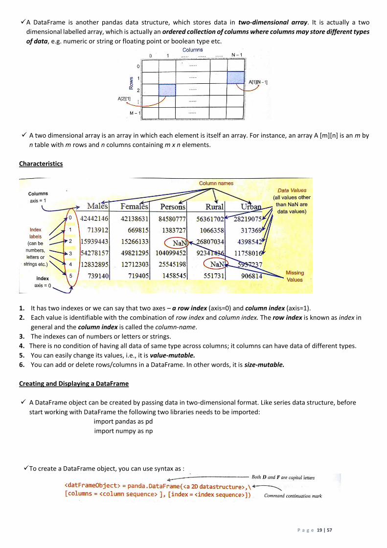
A DataFrame is another pandas data structure, which stores data in two-dimensional array. It is actually a two

dimensional labelled array, which is actually an ordered collection of columns where columns may store different types

of data, e.g. numeric or string or floating point or boolean type etc.

A two dimensional array is an array in which each element is itself an array. For instance, an array A [m][n] is an m by

n table with m rows and n columns containing m x n elements.

Characteristics

1. It has two indexes or we can say that two axes – a row index (axis=0) and column index (axis=1).

2. Each value is identifiable with the combination of row index and column index. The row index is known as index in

general and the column index is called the column-name.

3. The indexes can of numbers or letters or strings.

4. There is no condition of having all data of same type across columns; it columns can have data of different types.

5. You can easily change its values, i.e., it is value-mutable.

6. You can add or delete rows/columns in a DataFrame. In other words, it is size-mutable.

Creating and Displaying a DataFrame

A DataFrame object can be created by passing data in two-dimensional format. Like series data structure, before

start working with DataFrame the following two libraries needs to be imported:

import pandas as pd

import numpy as np

To create a DataFrame object, you can use syntax as :

P a g e 20 | 57

1. Creating a DataFrame Object from a 2-D Dictionary

A two dimensional dictionary is a dictionary having items as (key: value) where value part is a data structure of

any type : another dictionary, an ndarray, a Series object, a list etc. But here the value parts of all keys should

have similar structure and equal lengths.

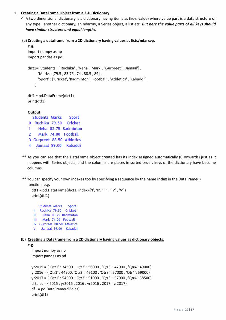
(a) Creating a dataframe from a 2D dictionary having values as lists/ndarrays

e.g.

import numpy as np

import pandas as pd

dict1={'Students': ['Ruchika' , 'Neha', 'Mark' , 'Gurpreet' , 'Jamaal'] ,

'Marks': [79.5 , 83.75 , 74 , 88.5 , 89] ,

'Sport' : ['Cricket', 'Badminton', 'Football' , 'Athletics' , 'Kabaddi'] ,

}

dtf1 = pd.DataFrame(dict1)

print(dtf1)

Output:

** As you can see that the DataFrame object created has its index assigned automatically (0 onwards) just as it

happens with Series objects, and the columns are places in sorted order. keys of the dictionary have become

columns.

** You can specify your own indexes too by specifying a sequence by the name index in the DataFrame( )

function, e.g.

dtf1 = pd.DataFrame(dict1, index=[‘I’, ‘II’, ‘III’ , ‘IV’ , ‘V’])

print(dtf1)

(b) Creating a DataFrame from a 2D dictionary having values as dictionary objects:

e.g.

import numpy as np

import pandas as pd

yr2015 = { 'Qtr1' : 34500 , 'Qtr2' : 56000 , 'Qtr3' : 47000 , 'Qtr4': 49000}

yr2016 = {'Qtr1' : 44900, 'Qtr2' : 46100 , 'Qtr3' : 57000 , 'Qtr4': 59000}

yr2017 = { 'Qtr1' : 54500 , 'Qtr2' : 51000 , 'Qtr3' : 57000 , 'Qtr4': 58500}

diSales = { 2015 : yr2015 , 2016 : yr2016 , 2017 : yr2017}

df1 = pd.DataFrame(diSales)

print(df1)

P a g e 21 | 57

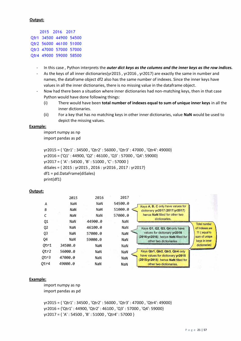
Output:

- In this case , Python interprets the outer dict keys as the columns and the inner keys as the row indices.

- As the keys of all inner dictionaries(yr2015 , yr2016 , yr2017) are exactly the same in number and

names, the dataframe object df2 also has the same number of indexes. Since the inner keys have

values in all the inner dictionaries, there is no missing value in the dataframe object.

- Now had there been a situation where inner dictionaries had non-matching keys, then in that case

Python would have done following things:

(i) There would have been total number of indexes equal to sum of unique inner keys in all the

inner dictionaries.

(ii) For a key that has no matching keys in other inner dictionaries, value NaN would be used to

depict the missing values.

Example:

import numpy as np

import pandas as pd

yr2015 = { 'Qtr1' : 34500 , 'Qtr2' : 56000 , 'Qtr3' : 47000 , 'Qtr4': 49000}

yr2016 = {'Q1' : 44900, 'Q2' : 46100 , 'Q3' : 57000 , 'Q4': 59000}

yr2017 = { 'A' : 54500 , 'B' : 51000 , 'C' : 57000 }

diSales = { 2015 : yr2015 , 2016 : yr2016 , 2017 : yr2017}


print(df1)

Output:

Example:

import numpy as np

import pandas as pd

yr2015 = { 'Qtr1' : 34500 , 'Qtr2' : 56000 , 'Qtr3' : 47000 , 'Qtr4': 49000}

yr2016 = {'Qtr1' : 44900, 'Qtr2' : 46100 , 'Q3' : 57000 , 'Q4': 59000}

yr2017 = { 'A' : 54500 , 'B' : 51000 , 'Qtr4' : 57000 }

P a g e 22 | 57

diSales = { 2015 : yr2015 , 2016 : yr2016 , 2017 : yr2017}


print(df1)

Output:

2. Creating a DataFrame Object from a 2-D ndarray

You can also pass a two-dimensional NumPy array to DataFrame( ) to create a dataframe object.

Example:

import numpy as np

import pandas as pd

narr1=np.array([[40,43,53],[64,55,46]],np.int32)

dtf1 = pd.DataFrame(narr1)

print(dtf1)

Output:

** As no keys are there, hence default names are given to indexes and columns, i.e. 0 onwards.

You can however, specify your own column names and/or index names by giving a columns sequence and/or

index sequence.

Example:

import numpy as np

import pandas as pd

narr1=np.array([[40,43,53],[64,55,46]],np.int32)

dtf1 = pd.DataFrame(narr1,columns=['First','Second','Three'], index=['A','B'])

print(dtf1)

Output:

If rows of ndarrays differ in length, i.e., if number of elements in each row differ, the Python will create just

single column in the dataframe object and the type of column will be considered as object.

P a g e 23 | 57

Example:

import numpy as np

import pandas as pd

narr1=np.array([[40,43],[64,55,46], [46.2,56.2]])

dtf1 = pd.DataFrame(narr1)

print(dtf1)

Output:

3. Creating a DataFrame object from a 2D dictionary with values as Series Object

Example:

import numpy as np

import pandas as pd

population=pd.Series([10927986,12691836,4631392,4328063],\

index=['Delhi', 'Mumbai','Kolkata','Chennai'])

AvgIncome = pd.Series([7216781092,8508781269,4226785362,5261784321],\


dict2 = {0 : population , 1 : AvgIncome}


print(dtf2)

Output:

** Dataframe object created (dtf2) has columns assigned from the keys of the dictionary object and its index

assigned from the indexes of the series objects which are the values of the dictionary object.

4. Creating a DataFrame Object from another DataFrame Object

Example:

import numpy as np

import pandas as pd







print(dtf2)

dtf3= pd.DataFrame(dtf2)

print(dtf3)

Single column created this time

because the lengths of rows of

ndarray did not match.

P a g e 24 | 57

Output:

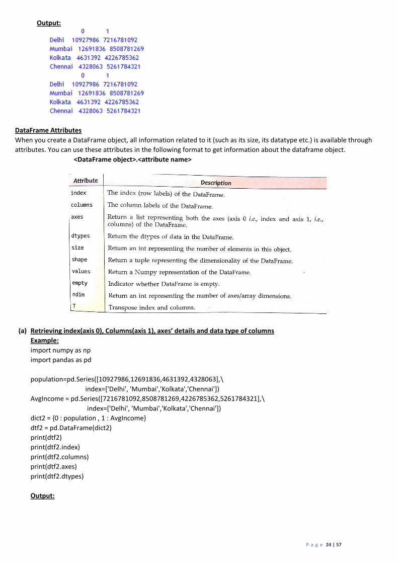
DataFrame Attributes

When you create a DataFrame object, all information related to it (such as its size, its datatype etc.) is available through

attributes. You can use these attributes in the following format to get information about the dataframe object.

<DataFrame object>.<attribute name>

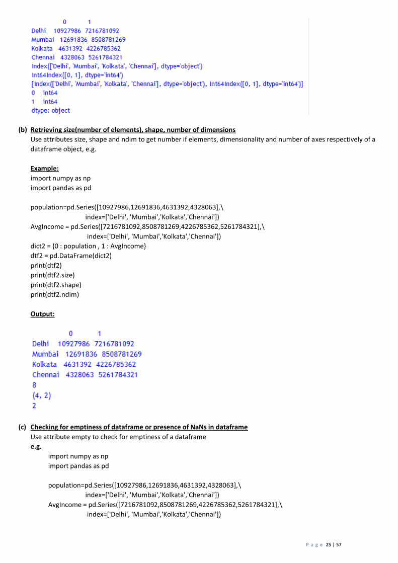
(a) Retrieving index(axis 0), Columns(axis 1), axes’ details and data type of columns

Example:

import numpy as np

import pandas as pd







print(dtf2)

print(dtf2.index)

print(dtf2.columns)

print(dtf2.axes)

print(dtf2.dtypes)

Output:

P a g e 25 | 57

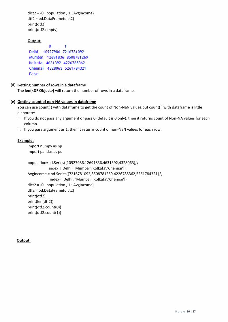
(b) Retrieving size(number of elements), shape, number of dimensions

Use attributes size, shape and ndim to get number if elements, dimensionality and number of axes respectively of a

dataframe object, e.g.

Example:

import numpy as np

import pandas as pd







print(dtf2)

print(dtf2.size)

print(dtf2.shape)

print(dtf2.ndim)

Output:

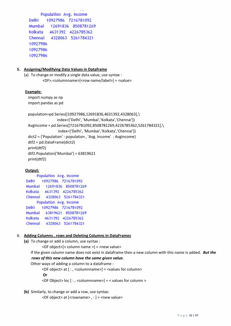
(c) Checking for emptiness of dataframe or presence of NaNs in dataframe

Use attribute empty to check for emptiness of a dataframe

e.g.

import numpy as np

import pandas as pd





P a g e 26 | 57



print(dtf2)

print(dtf2.empty)

Output:

(d) Getting number of rows in a dataframe

The len(<DF Object>) will return the number of rows in a dataframe.

(e) Getting count of non-NA values in dataframe

You can use count( ) with dataframe to get the count of Non-NaN values,but count( ) with dataframe is little

elaborate:

I. If you do not pass any argument or pass 0 (default is 0 only), then it returns count of Non-NA values for each

column.

II. If you pass argument as 1, then it returns count of non-NaN values for each row.

Example:

import numpy as np

import pandas as pd







print(dtf2)

print(len(dtf2))

print(dtf2.count(0))

print(dtf2.count(1))

Output:

P a g e 27 | 57

(f) Transposing a Dataframe

You can transpose a dataframe by swapping its indexes and columns by using attribute T ,

e.g.

import numpy as np

import pandas as pd







print(dtf2)

print(dtf2.T)

Output:

SELECTING OR ACCESSING DATA

1. Selecting/Accessing a Column

Single column at a time

<DataFrame object> [<Column name>]

Or

<DataFrame object>.<Column name>

Multiple columns at a time

<DataFrame object>[ [columnname , columnname, ……….]]

P a g e 28 | 57

Example:

import numpy as np

import pandas as pd





dict2 = {'Population' : population , 'Avg. Income' : AvgIncome}


print(dtf2)

print("========")

print(dtf2.Population)

print("========")

print(dtf2[['Population','Avg. Income']])

Output:

2. Selecting/Accessing a SubSet from a Dataframe using Row/Column Name

For this purpose, you can use following syntax to select/access a subset from a dataframe object:

<DataFrameObject>.loc [<startrow>: <endrow>, <startcolumn> :<endcolumn>]

I. To access a row, just give the row name/label as this : <DF Object>.loc[<row label> , : ]

Make sure not to miss the COLON AFTER COMMA.

II. To access multiple rows, use : <DF object>.loc[<start row> :<endrow>, : ]

Make sure not to miss the COLON AFTER COMMA.

III. To access selective columns, use : <DF object>.loc[ : , <start column> , <end column>]

IV. To access a range of columns from a range of rows, use:

<DF object>.loc [<startrow>: <endrow>, <startcolumn> :<endcolumn>]

Example:

P a g e 29 | 57

import numpy as np

import pandas as pd







print(dtf2)

print("==Accessing Single row==")

print(dtf2.loc['Delhi' , :])

print(dtf2.loc['Kolkata' ,:])

print("==Accessing Multiple rows==")

print(dtf2.loc['Mumbai' : 'Chennai' , :])

print("==Accessing Columns==")

print(dtf2.loc[ : , 'Population'])

print("==Accessing range of columns and rows==")

print(dtf2.loc['Delhi' : 'Mumbai' , 'Population' : 'Avg. Income'])

Output:

3. Obtaining a Subset/Slice from a Dataframe using Row/Column Numeric Index/Position

Sometimes your dataframe object does not contain row or column labels or even you may not remember them.

In such cases, you can extract subset from dataframe using the row and column numeric index/position, but this

time you will use iloc instead of loc. iloc means integer location.

<DF object>.iloc[<startrow index>: <endrow index>, <startcolumn index> :<endcolumn index>]

P a g e 30 | 57

** endindex is excluded here.

Example:

import numpy as np

import pandas as pd







print(dtf2)

print(dtf2.iloc[0:2,0:1])

Output:

4. Selecting/Accessing Individual Value

(i) Either give name of row or numeric index in square brackets with, i.e., as this :

<DF object>.<column>[<row name or row numeric index>]

(ii) You can use at or iat attribute with DF object as shown below:

<DF object>.at [<row name>, <column name>]

Or

<DF object>. iat [<numeric row index>, <numeric column index>]

Example:

import numpy as np

import pandas as pd







print(dtf2)

print(dtf2.Population['Delhi'])

print(dtf2.at['Delhi', 'Population'])

print(dtf2.iat[0,0])

Output:

P a g e 31 | 57

5. Assigning/Modifying Data Values in Dataframe

(a) To change or modify a single data value, use syntax :

<DF>.<columnname>[<row name/label>] = <value>

Example:

import numpy as np

import pandas as pd







print(dtf2)

dtf2.Population['Mumbai'] = 63819621

print(dtf2)

Output:

6. Adding Columns , rows and Deleting Columns in DataFrames

(a) To change or add a column, use syntax :

<DF object>[< column name >] = <new value>

If the given column name does not exist in dataframe then a new column with this name is added. But the

rows of this new column have the same given value.

Other ways of adding a column to a dataframe :

<DF object> at [ : , <columnname>] = <values for column>

Or

<DF Object> loc [ : , <columnname>] = < values for column >

(b) Similarly, to change or add a row, use syntax:

<DF object> at [<rowname> , : ] = <new value>

P a g e 32 | 57

Or

<DF Object> loc [<row name> , : ] = <new value>

Likewise, if there is no row with such row label , then Python adds new row with this row label and assigns

given values to all its columns. But the columns of this new row have the same given value.

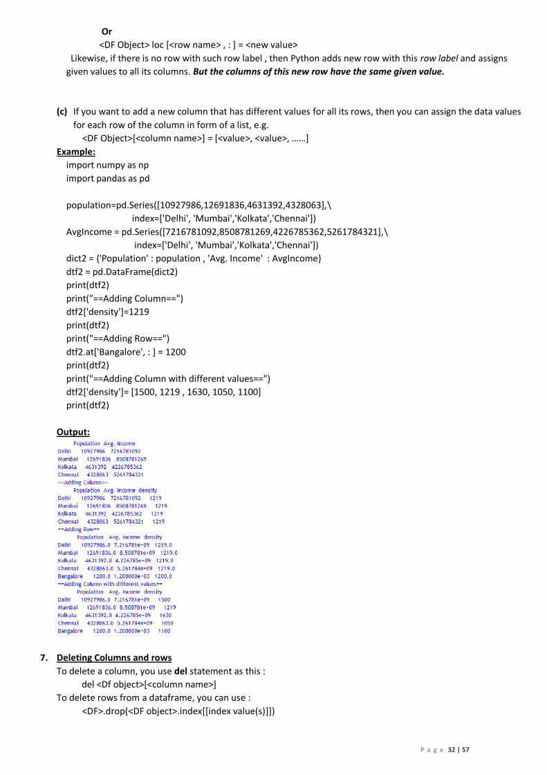
(c) If you want to add a new column that has different values for all its rows, then you can assign the data values

for each row of the column in form of a list, e.g.

<DF Object>[<column name>] = [<value>, <value>, ……]

Example:

import numpy as np

import pandas as pd







print(dtf2)

print("==Adding Column==")

dtf2['density']=1219

print(dtf2)

print("==Adding Row==")

dtf2.at['Bangalore', : ] = 1200

print(dtf2)

print("==Adding Column with different values==")

dtf2['density']= [1500, 1219 , 1630, 1050, 1100]

print(dtf2)

Output:

7. Deleting Columns and rows

To delete a column, you use del statement as this :

del <Df object>[<column name>]

To delete rows from a dataframe, you can use :

<DF>.drop(<DF object>.index[[index value(s)]])

P a g e 33 | 57

e.g.

import numpy as np

import pandas as pd







print("Dataframe before deletion of column")

dtf2['density']= [1500, 1219 , 1630, 1050]

print(dtf2)

print("Dataframe after deletion of column")

del dtf2['density']

print(dtf2)

print("Dataframe after deletion of first and third row")

print(dtf2.drop(dtf2.index[[0,2]]))

Output:

ITERATING OVER A DATAFRAME

Two methods are used for iterating over a given dataframe:

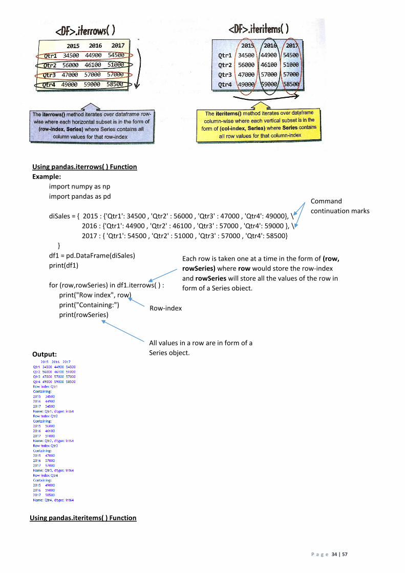
1. The method <DF>.iterrows( ) views a dataframe in the form of horizontal subsets i.e., row-wise. Each horizontal

subset is in the form of (row index, Series) where Series contains all column values for that row-index.

2. The method <DF>.iteritems( ) views a dataframe in the form of vertical subsets i.e., column-wise. Each vertical

subset is in the form of (col-index, Series) where Series contains all row values for that column-index.

P a g e 34 | 57

Using pandas.iterrows( ) Function

Example:

import numpy as np

import pandas as pd

diSales = { 2015 : {'Qtr1': 34500 , 'Qtr2' : 56000 , 'Qtr3' : 47000 , 'Qtr4': 49000}, \

2016 : {'Qtr1': 44900 , 'Qtr2' : 46100 , 'Qtr3' : 57000 , 'Qtr4': 59000 }, \

2017 : { 'Qtr1': 54500 , 'Qtr2' : 51000 , 'Qtr3' : 57000 , 'Qtr4': 58500}

}


print(df1)

for (row,rowSeries) in df1.iterrows( ) :

print("Row index", row)

print("Containing:")

print(rowSeries)

Output:

Using pandas.iteritems( ) Function

Command

continuation marks

Each row is taken one at a time in the form of (row,

rowSeries) where row would store the row-index

and rowSeries will store all the values of the row in

form of a Series object.

Row-index

All values in a row are in form of a

Series object.

P a g e 35 | 57

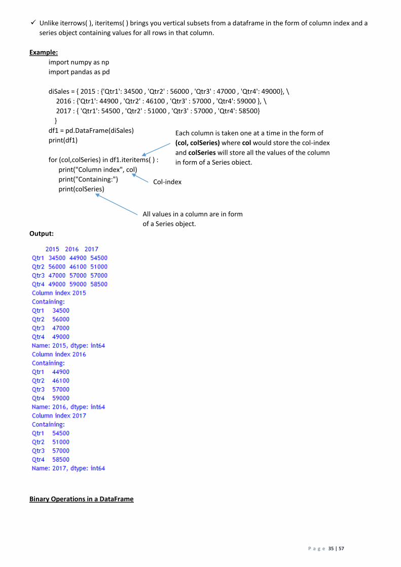
Unlike iterrows( ), iteritems( ) brings you vertical subsets from a dataframe in the form of column index and a

series object containing values for all rows in that column.

Example:

import numpy as np

import pandas as pd

diSales = { 2015 : {'Qtr1': 34500 , 'Qtr2' : 56000 , 'Qtr3' : 47000 , 'Qtr4': 49000}, \

2016 : {'Qtr1': 44900 , 'Qtr2' : 46100 , 'Qtr3' : 57000 , 'Qtr4': 59000 }, \

2017 : { 'Qtr1': 54500 , 'Qtr2' : 51000 , 'Qtr3' : 57000 , 'Qtr4': 58500}

}


print(df1)

for (col,colSeries) in df1.iteritems( ) :

print("Column index", col)

print("Containing:")

print(colSeries)

Output:

Binary Operations in a DataFrame

Each column is taken one at a time in the form of

(col, colSeries) where col would store the col-index

and colSeries will store all the values of the column

in form of a Series object.

Col-index

All values in a column are in form

of a Series object.

P a g e 36 | 57

In a binary operation, the data from the two dataframes are aligned on the bases of their row and

column indexes and for matching row, column index, the given operation is performed and for

non-matching row, column indexes NaN value is stored in the result.

You can perform add binary operation on two dataframe objects using either + operator or using

add( ) as per syntax: <DF1>.add(<DF2>) which means <DF1>+<DF2> or by using radd( ) i.e., reverse

add as per syntax: <DF1>.radd(<DF2>) which means <DF2>+<DF1>

You can perform subtract binary operation on two dataframe objects using either – (minus)

operator or using sub( ) as per syntax: <DF1>.sub(<DF2>) which means <DF1> - <DF2> or by using

rsub( ) i.e., reverse subtract as per syntax: <DF1>.rsub(<DF2>) which means <DF2> - <DF1>

You can perform multiply binary operation on two dataframe objects using either * operator or

using mul( ) as per syntax : <DF>.mul(<DF>)

You can perform division binary operation on two dataframe objects using either / operator or

using div( ) as per syntax : <DF>.div(<DF>)

Example:

import numpy as np

import pandas as pd

d1 = { 'A' : [1,4,7], 'B' : [2,5,8] , 'C' : [3, 6 ,9]}

df1 = pd.DataFrame(d1)

d2 = { 'A' : [10,40,70], 'B' : [20,50,80] , 'C' : [30, 60 ,90]}


d3 = { 'A' : [100,400], 'B' : [200,500] , 'C' : [300, 600]}


d4 = { 'A' : [1000,4000,7000], 'B' : [2000,5000,8000]}


print(df1)

print(df2)

print(df3)

print(df4)

print("==Addition Operation==")

print(df1+df2)

print(df1.add(df3))

print(df1+df4)

print("==Subtraction Operation==")

print(df1-df2)

print(df1.sub(df3))

print(df1-df4)

print("==Multiply Operation==")

print(df1*df2)

print(df1.mul(df3))

print(df1*df4)

P a g e 37 | 57

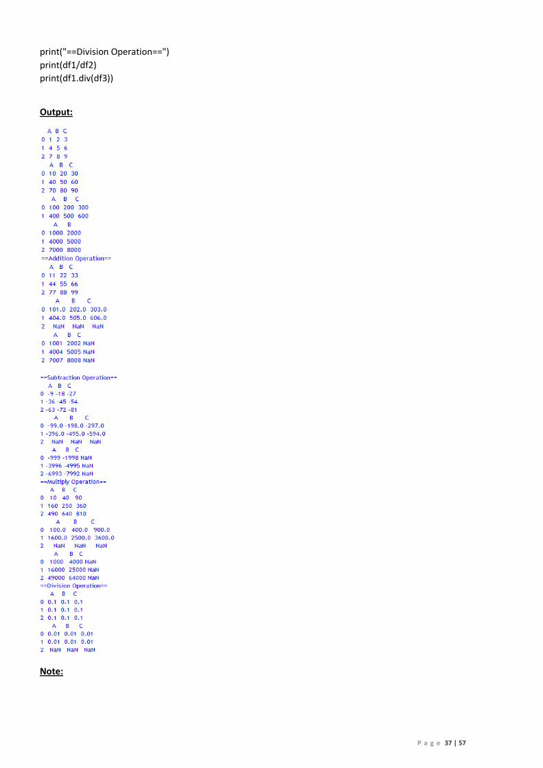
print("==Division Operation==")

print(df1/df2)

print(df1.div(df3))

Output:

Note:

P a g e 38 | 57

* results of df1+df3 have the sum values displayed as float numbers. The reason behind it is that whenever any

column of a dataframe has a NaN value in it, then its type is automatically changed to floating point because in

Python integer types cannot store NaN values.

* df1 – df2 is equal to df1.sub(df2) but df2 – df1 is equal to df1.rsub(df2)

* when + is performed on string values, it concatenates them.

* data type of values in dataframe should be binary operator compatible.

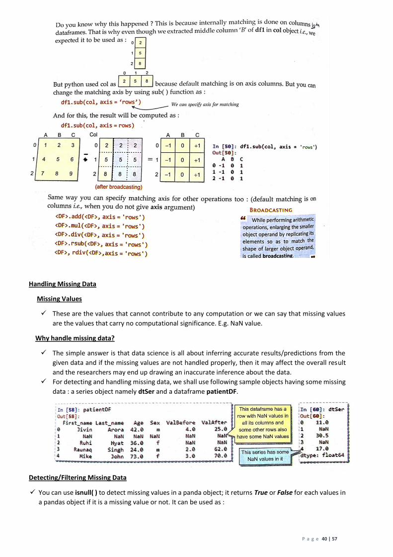
Matching and Broadcasting Operations

While performing arithmetic operations on dataframes, data is aligned on the basis of matching indexes and then

performed arithmetic ; for non-overlapping indexes, the arithmetic operations result as a NaN(Not a Number). This

default behaviour of data alignment on the basis of matching indexes is called MATCHING.

BROADCASTING

BROADCASTING IN DATAFRAMES

P a g e 39 | 57

Given below are two dataframes(namely row and col ) that are created by extracting middle row

and middle column respectively from the above shown dataframe df1.

Let us see how these will perform an arithmetic operation say subtraction with df1. That is, what

will be produced by df1 – row (or df1.sub(row)) and df1 – col (or df1.sub(col))

Let us check how df1 – col or df1.sub(col) will be performed.

will internally transform to

P a g e 40 | 57

Handling Missing Data

Missing Values

These are the values that cannot contribute to any computation or we can say that missing values

are the values that carry no computational significance. E.g. NaN value.

Why handle missing data?

The simple answer is that data science is all about inferring accurate results/predictions from the

given data and if the missing values are not handled properly, then it may affect the overall result

and the researchers may end up drawing an inaccurate inference about the data.

For detecting and handling missing data, we shall use following sample objects having some missing

data : a series object namely dtSer and a dataframe patientDF.

Detecting/Filtering Missing Data

You can use isnull( ) to detect missing values in a panda object; it returns True or False for each values in

a pandas object if it is a missing value or not. It can be used as :

P a g e 41 | 57

<PandaObject>.isnull( )

<PandaObject> means it is applicable to both Series as well as DataFrame objects.

Consider the following outputs:

If you want to filter data which is not a missing value i.e., non-null data, then you can use following

for Series object:

<Series object>[SeriesObject.notnull( )]

E.g.

** The above method will not work for a dataframe object.

Handling Missing Data – Dropping Missing Values

To drop missing values you can use dropna( )in following three ways:

(a) <PandaObject>.dropna( )

This will drop all the rows that have NaN values in them, even row with a single NaN value in it, e.g.

(b) <DF>.dropna(how=’all’)

With argument how=’all’ , it will drop only those rows that have all NaN values, i.e. , no value is non-

null in those rows, e.g.

(c) <DF>.dropna(axis=1)

P a g e 42 | 57

With argument axis =1 , will drop columns that have any NaN values in them, e.g.

Handling Missing Data – Filling Missing Values

Though dropna( ) removes the null values, but you can lose other non-null data with it too. To avoid this,

you may want to fill the missing data with some appropriate value of your choice. For this purpose you

can use fillna( ) in following ways:

(a) <PandaObject>.fillna(<n>)

This will fill all NaN values in a pandas object with the given <n> value, e.g.

(b) Using dictionary with fillna( ) to specify fill values for each column separately

You can create a dictionary that defines fill values for each of the columns. And then you can pass this

dictionary as an argument to fillna( ), Pandas will fill the specified value for each column defined in the

dictionary. It will leave those columns untouched or unchanged that are not in the dicntionary.

The syntax to use this format of fillna( ) is :

<DF>.fillna(<dictionary having fill values for columns>)

e.g.

More operations with Pandas Objects

P a g e 43 | 57

1. Comparisons of Pandas Object

For understanding this thing we are using following objects:

Normal comparison operators can be used as shown below:

Now, look carefully another add operation on dfc1 and dfc3 objects.

Even though you see both results(extreme left and extreme right above) are just the same, their

comparison returned False for some value. The reason behind it is that : NaN values do not compare

as equals.

To compare objects having NaN values, it is better to use equals( ) that returns True if two NaN

values are compared for equality. E.g.

Similarly, you can compare pandas objects with scalar values ; use equals( ) if the values involve

NaNs :

P a g e 44 | 57

** For comparison, two DataFrame objects should match in lengths and in columns.

2. Comparing Series

Comparison of two series objects is also based on same points as Dataframe:

For comparison, two Series objects should match in lengths and in indexes.

NaN values cannot be compared using comparison operators.

equals( ) results in True while comparing two NaN values.

Boolean Reductions

P a g e 45 | 57

With Boolean reduction, you can get the overall result of a row or column with a single True or False.It

summarize the Boolean result for an axis. For this purpose Pandas offers following Boolean reduction

functions or attributes:

1. empty – this attribute is indicator whether a DataFrame is empty. It is used as :

<DF>.empty

Pandas will return True or False if a dataframe is empty or not, e.g.

An empty dataframe does not contain any value, not even NaN; a dataframe having all NaN value

is also not considered empty. E.g.

2. any( ) – This function returns True if any element is True over requested axis, By default ,it checks if any

value in a column(default axis 0) meets this criteria, if it does it returns True, i.e., if any of the values along

the specified axis is True, this will return True. It is used as per following syntax:

<DataFrame comparison result object>.any(axis=None)

3. all( ) – Unlike any( ), the all( ) will return True/False if only all the values on an axis are True or False

according to given comparison. It is used as per syntax:

<DataFrame comparison result object>.any(axis=None)

P a g e 46 | 57

Combining DataFrames

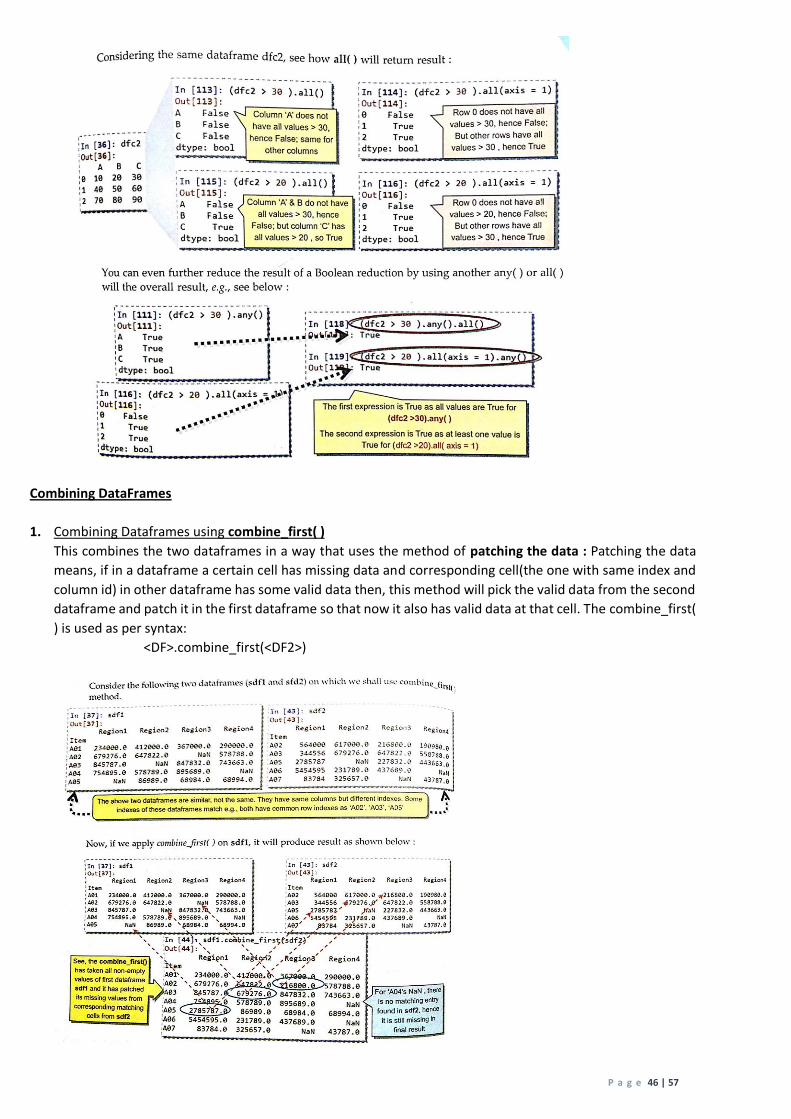
1. Combining Dataframes using combine_first( )

This combines the two dataframes in a way that uses the method of patching the data : Patching the data

means, if in a dataframe a certain cell has missing data and corresponding cell(the one with same index and

column id) in other dataframe has some valid data then, this method will pick the valid data from the second

dataframe and patch it in the first dataframe so that now it also has valid data at that cell. The combine_first(

) is used as per syntax:

<DF>.combine_first(<DF2>)

P a g e 47 | 57

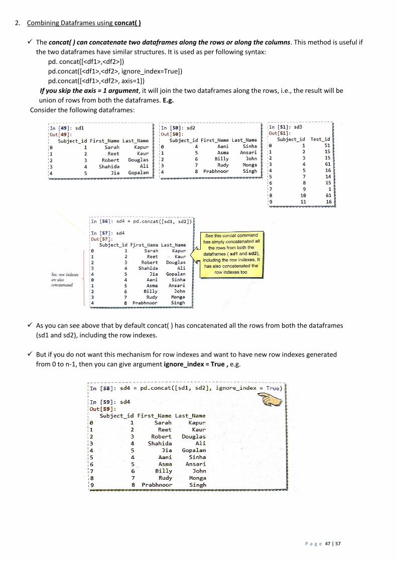
2. Combining Dataframes using concat( )

The concat( ) can concatenate two dataframes along the rows or along the columns. This method is useful if

the two dataframes have similar structures. It is used as per following syntax:

pd. concat([<df1>,<df2>])

pd.concat([<df1>,<df2>, ignore_index=True])

pd.concat([<df1>,<df2>, axis=1])

If you skip the axis = 1 argument, it will join the two dataframes along the rows, i.e., the result will be

union of rows from both the dataframes. E.g.

Consider the following dataframes:

As you can see above that by default concat( ) has concatenated all the rows from both the dataframes

(sd1 and sd2), including the row indexes.

But if you do not want this mechanism for row indexes and want to have new row indexes generated

from 0 to n-1, then you can give argument ignore_index = True , e.g.

P a g e 48 | 57

By default it concatenates along the rows; to concatenate along the column, you can give argument axis

= 1 as shown below:

3. Combining Dataframes using merge( )

Sometimes, you would want to combine two dataframes such that two rows with some common value

are merged together in the final result. For this, Pandas provides merge( ) function in which you can specify

the field on the basis of which you want to combine the two dataframes. It is used as per syntax:

pd.merge(<DF1>,<DF2> )

pd.merge(<DF1>,<DF2>, on=<field_name>)

If you skip the argument on=<field_name> , then it will take any merge on common fields of the two

dataframes but you can explicitly specify the field on the basis of which you want to merge the two

dataframes.

E.g.

***********************

P a g e 49 | 57

CHAPTER 12 – DATA TRANSFER BETWEEN FILES, SQL DATABASES AND DATAFRAMES

Transferring Data between .csv Files and DataFrames

The acronym CSV is short for Comma Separated Values. The CSV format refers to a tabular data that has been

saved as plaintext where data is separated by commas.

In CSV format:

1. Each row of the table is stored in one row i.e, the number of rows in a CSV file are equal to number of

rows in the table.

2. The field-values of a row are stored together with commas after every field value; but after the last

field’s value in a line/row, no comma is given, just the end of line.

Advantages of CSV format

A simple, compact and ubiquitous format for data storage.

A common format for data interchange.

It can be opened in popular spreadsheet packages like MS-Excel, Calc etc.

Nearly all spreadsheets and databases support import/export to csv format.

Loading Data from CSV to Dataframes

Python’s Pandas library offers two functions read_csv( ) and to_csv( ) that help you bring data from a CSV file

into a dataframe and write a dataframe’s data to a CSV file.

Suppose we have following CSV file – sample.csv, shown in notepad as well as in MS Excel.

Before doing anything with Pandas, like always, make sure to import the Pandas library by giving command:

import pandas as pd

Reading From a CSV File to Dataframe

You can use read_csv( ) function to read data from a CSV file in your dataframe by using the function as per

following syntax:

<DF> = pandas.read_csv(<filepath>)

That is, if you give following command after importing pandas library(suppose sample file is stored in c:\data

folder):

df = pd.read_csv(“c:\\data\\sample.csv“)

Now if you print dataframe df, Python will show:

P a g e 50 | 57

Reading CSV File and Specifying Own Column Names

Case I :

But you may have a CSV file that does not have top row containing column headers(as shown below):

Now if you read such a file by just giving the filepath, it will take the top row as the column headers, eg., as

shown below:

df2 = pd.read_csv(“c:\\data\\mydata.csv”)

Now if you print dataframe df2, Python will show :

But the top row (1, Sarah, Kapur) is data, not column headings. For such a situation, you can specify own

column heading in read_csv( ) using names argument as per following syntax:

<DF> = pandas.read_csv(<filepath> , names=<sequence containing column names>)

That is, you need to modify above statement as :

df2 = pd.read_csv(“c:\\data\\mydata.csv”, names=[“Roll_no”, “First_Name”,”Last_Name”])

And now when you print df2, Python will show:

P a g e 51 | 57

Case II:

If you want the first row not to be used as header and at the same time you do not want to specify column

headings rather go with default column headings which go like 0,1, 2, 3, ………., then simply give argument as

header=None in read_csv( ), i.e., as:

<DF> = pandas.read_csv(<filepath>, header=None)

For example, the following statement will not consider row 1 for column heading and default column headings will

be taken.

df3 = pd.read_csv(“c:\\data\\mydata.csv”, header=None)

The dataframe df3 will be storing data as shown below:

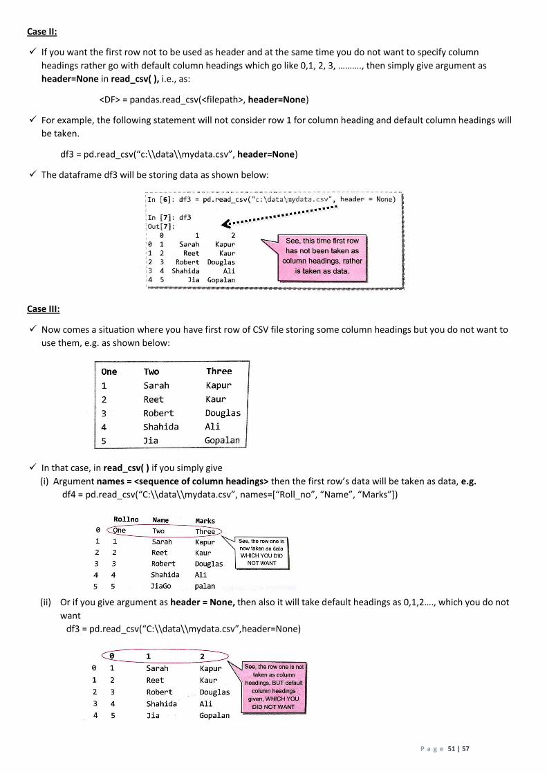
Case III:

Now comes a situation where you have first row of CSV file storing some column headings but you do not want to

use them, e.g. as shown below:

In that case, in read_csv( ) if you simply give

(i) Argument names = <sequence of column headings> then the first row’s data will be taken as data, e.g.

df4 = pd.read_csv(“C:\\data\\mydata.csv”, names=[“Roll_no”, “Name”, “Marks”])

(ii) Or if you give argument as header = None, then also it will take default headings as 0,1,2…., which you do not

want

df3 = pd.read_csv(“C:\\data\\mydata.csv”,header=None)

P a g e 52 | 57

The solution to this problem is to find a way so that it skips row 1 while fetching data from CSV file.For this, you

need to give two arguments along with file path : one for column headings i.e., names=<column headings

sequence> and another skiprows = <n> , i.e.,

<DF> = pandas.read_csv(<filepath>, names =<column names sequence>, skiprows=<n> )

The number given with skip rows tells how many rows to be skipped from CSV while reading data. Thus, if you give

statement as given below:

Reading Specified Number of Rows from CSV file

Given argument nrows =<n> in read_csv( ), will read the specified number of rows from the CSV file, e.g.

Reading from CSV files having Separator Different from Comma

Some CSV files are so created that their separator character is different from comma such as a semicolon( ;) or a pipe

symbol (|) etc. To read data from such CSV files, you need to specify an additional argument as sep=<separator

character>. If you skip this argument then default separator character(comma) is considered.

e.g.

Storing Dataframe’s Data to CSV File

For this purpose, Python Pandas provides to_csv( ) function that saves the data of a dataframe in a CSV file.

Function to_csv( ) can be used as per following syntaxes:

<DF>.to_csv(<filepath>)

Or

<DF>.to_csv(<filepath>, sep=<separator_character> )

** The separator character must be a one character string only.

P a g e 53 | 57

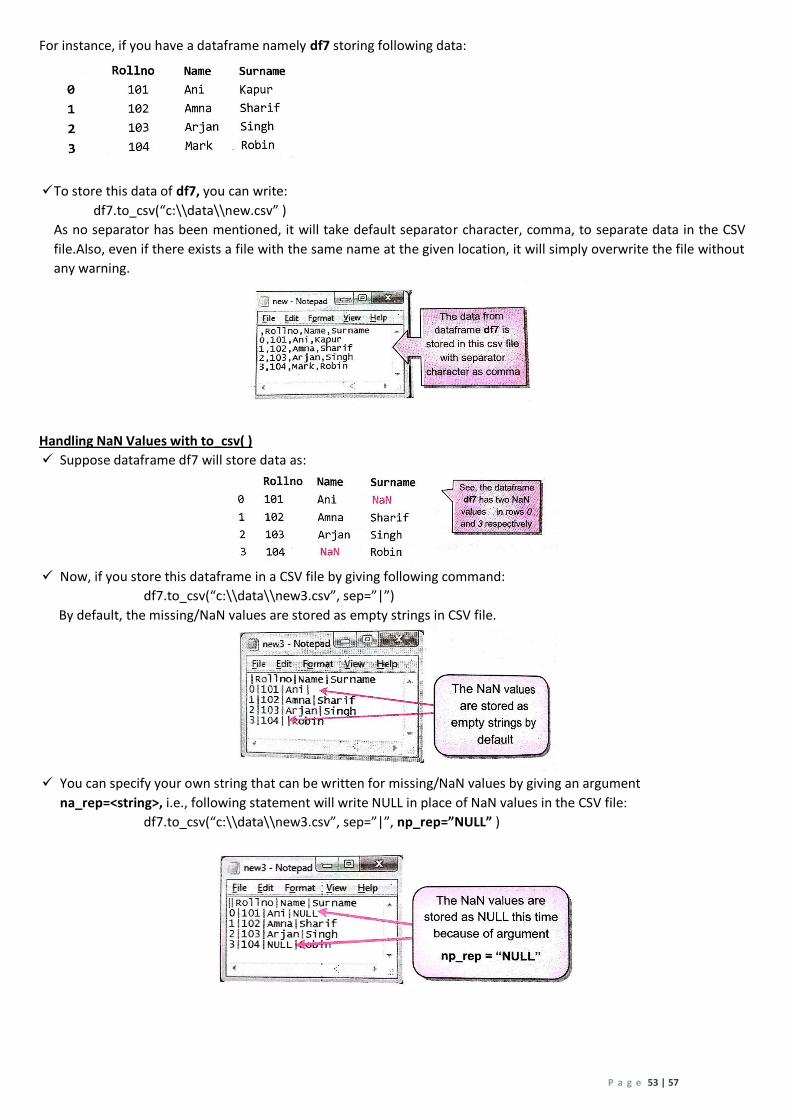
For instance, if you have a dataframe namely df7 storing following data:

To store this data of df7, you can write:

df7.to_csv(“c:\\data\\new.csv” )

As no separator has been mentioned, it will take default separator character, comma, to separate data in the CSV

file.Also, even if there exists a file with the same name at the given location, it will simply overwrite the file without

any warning.

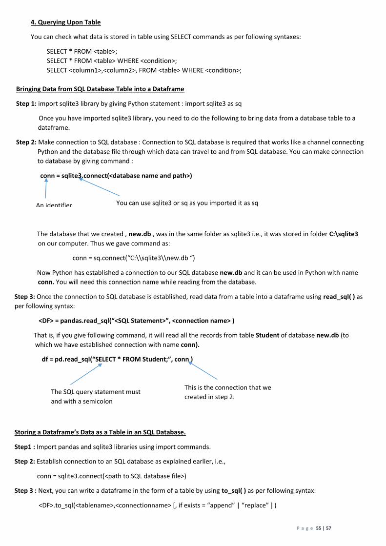
Handling NaN Values with to_csv( )

Suppose dataframe df7 will store data as:

Now, if you store this dataframe in a CSV file by giving following command:

df7.to_csv(“c:\\data\\new3.csv”, sep=”|”)

By default, the missing/NaN values are stored as empty strings in CSV file.

You can specify your own string that can be written for missing/NaN values by giving an argument

na_rep=<string>, i.e., following statement will write NULL in place of NaN values in the CSV file:

df7.to_csv(“c:\\data\\new3.csv”, sep=”|”, np_rep=”NULL” )

P a g e 54 | 57

Transferring Data Between Dataframes and SQL Databases

1. SQL Databases- relational database- data stored in realtions(tables)- make use of SQL commands. E.g. MySQL

2. Here we will learn to store data into an SQL based table and to read data from an SQL based table using a Python’s

linrary sqlite3 that is by default bundled with Python.

SQLite Database

It is an embedded SQL database engine, which implements a relational database management system that

is self-contained , serverless and requires zero configuration.

It is in public domain and is freely available for any type of use.

It can be downloaded from SQLite’s download page: www.sqlite.org/download.html

COMMANDS UNDER SQLITE

1. Creating Database in sqlite

.open <databasename>.db

This command works in two ways:

If the given database does not exist, sqlite will create one and then open it for processing.

If the given database exists, sqlite will open the database for processing.

2. Creating Table

To create a table, you can write SQL statement CREATE TABLE as per following syntax:

CREATE TABLE <table name> (

<column1> <datatype> <constraint>,

<column2> <datatype> <constraint>,

…………

) ;

You can use any of the following, most common data types:

INTEGER – for non-fractional numbers, whole numbers

TEXT – for storing text,alphabets,alphanumeric data

REAL – for storing fractional numbers i.e., numbers with decimals

CHAR(<n>) – for storing exact number of characters in a field.

Following SQL command will create a basic table namely student:

Sqlite > CREATE TABLE student(

Rollno INTEGER NOT NULL PRIMARY KEY,

Name TEXT NOT NULL,

Marks REAL ) ;

You can give .tables command on sqlite prompt to see if the table has been created in your database

i.e.,

Sqlite > . tables

3. Insert Data in Table

You can insert data in an existing table using SQL command INSERT INTO as per following syntax:

INSERT INTO <tablename>

VALUES(<value for column1>, <value for column2>…..) ;

For example, following command will add a record in our Student table that we created just before:

Sqlite > INSERT INTO Student

VALUES(1001, “Esha”, 67.5);

http://www.sqlite.org/download.html

P a g e 55 | 57

4. Querying Upon Table

You can check what data is stored in table using SELECT commands as per following syntaxes:

SELECT * FROM <table>;

SELECT * FROM <table> WHERE <condition>;

SELECT <column1>,<column2>, FROM <table> WHERE <condition>;

Bringing Data from SQL Database Table into a Dataframe

Step 1: import sqlite3 library by giving Python statement : import sqlite3 as sq

Once you have imported sqlite3 library, you need to do the following to bring data from a database table to a

dataframe.

Step 2: Make connection to SQL database : Connection to SQL database is required that works like a channel connecting

Python and the database file through which data can travel to and from SQL database. You can make connection

to database by giving command :

conn = sqlite3.connect(<database name and path>)

The database that we created , new.db , was in the same folder as sqlite3 i.e., it was stored in folder C:\sqlite3

on our computer. Thus we gave command as:

conn = sq.connect(“C:\\sqlite3\\new.db “)

Now Python has established a connection to our SQL database new.db and it can be used in Python with name

conn. You will need this connection name while reading from the database.

Step 3: Once the connection to SQL database is established, read data from a table into a dataframe using read_sql( ) as

per following syntax:

<DF> = pandas.read_sql(“<SQL Statement>”, <connection name> )

That is, if you give following command, it will read all the records from table Student of database new.db (to

which we have established connection with name conn).

df = pd.read_sql(“SELECT * FROM Student;”, conn )

Storing a Dataframe’s Data as a Table in an SQL Database.

Step1 : Import pandas and sqlite3 libraries using import commands.

Step 2: Establish connection to an SQL database as explained earlier, i.e.,

conn = sqlite3.connect(<path to SQL database file>)

Step 3 : Next, you can write a dataframe in the form of a table by using to_sql( ) as per following syntax:

<DF>.to_sql(<tablename>,<connectionname> [, if exists = “append” | “replace” ] )

An identifier You can use sqlite3 or sq as you imported it as sq

The SQL query statement must

and with a semicolon

This is the connection that we

created in step 2.

P a g e 56 | 57

If you run to_sql( ) that has a table name which already exists then you must specify argument if_exist =”append”

or if_exists = “replace” otherwise Python will give ERROR. If you set the value as “append” , then new data will be

appended to existing table and if you set the value as “replace” then new data will replace the old data in given

table.

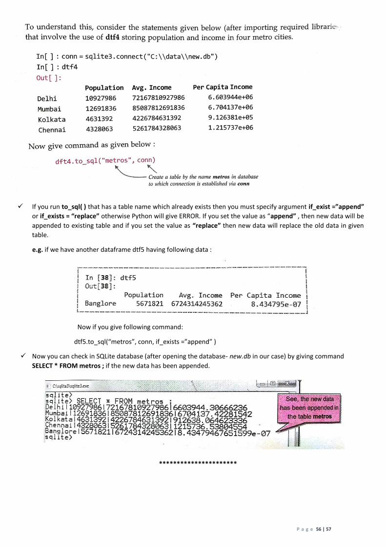
e.g. if we have another dataframe dtf5 having following data :

Now if you give following command:

dtf5.to_sql(“metros”, conn, if_exists =”append” )

Now you can check in SQLite database (after opening the database- new.db in our case) by giving command

SELECT * FROM metros ; if the new data has been appended.

**********************

P a g e 57 | 57

Chapter 10 – Introducing Python Pandas (Question Bank)

Q1. What is the use of Python Pandas library?

Q2. What are ndarrays? How are they different from Python lists?

Q3. What are axes in a numpy array?

Q4. To create a sequence of numbers, NumPy provides a function namely ____________that works like

range( ) but returns arrays instead of lists.

Q5. In NumPy arrays, dimensions are called__________ and number of axes is called ______________.

Q6. Can you duplicate indexes in a series object?

Q7. What do these attributes of series signify? (a) size (b) itemsize (iii) nbytes

Q8. If S1 is a series object then how will len(S1) and S1.count( ) behave?

Q9. Write commands to create following data structures, each having three integer elements 3,4,5 :

(a) ndarray (b) list (c) series

Q10. What are NaNs? How do you store them in a datastructures?

Q11. True/False. Series object always have indexes 0 to n-1.

Q12. Given a Series that stores the area of some states in km2 . Write code to find out the biggest and smallest

three areas from the given Series. Given Series has been created like this:

Ser1 = pd.Series([34567,

890,450,67892,34677,78902,256711,678291,637632,25723,2367,11789,345,256517] )

Q13. Given are two objects, a list object namely lst1 and a Series object namely ser1, both are having similar

values i.e., 2, 4 , 6, 8. Find out the output produced by following statements:

(i) print(lst1 * 2) (ii) print(ser1 * 2 )

Q14. Can you specify the reason behind the output produced by the code statements of previous question?

Q15. From the series of areas (given earlier that stores areas of states in km2 ), find out the areas that are

more than 50000 km2 .

**************************