Emissions from residential Emissions from residential energy useenergy use

Chandra VenkataramanDepartment of Chemical EngineeringIndian Institute of Technology, Bombay

TF HTAP Emissions Inventory and Future Projections Workshop

October 18-20, 2006, Beijing

AcknowledgmentsAcknowledgments

•Organizers: for invitation / hospitality and defining workshop issues.

•Collaborators: Gazala Habib, Shekar Reddy, ShubhaVerma, Manish Shrivastava, Baban Wagh, IIT Bombay; Antonio Miguel, Arantza Fernandez, Sheldon Friedlander, UCLA; Tami Bond, UIUC; Jamie Schauer, U Wisc Madison.

•Funding Support: ISRO-GBP, MHRD.

• The source of the problem (or problem with the source).• Emitted pollutants of regional / global

relevance.• Inventory methodology.• Uncertainties and their containment (more than

mere reduction).• Transport pathways – South Asia.• Recommendations.

OutlineOutline

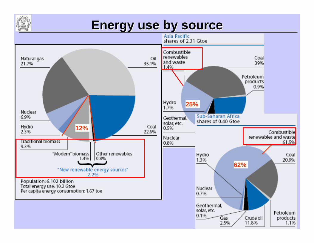
Energy use by sourceEnergy use by source

12%

25%

62%

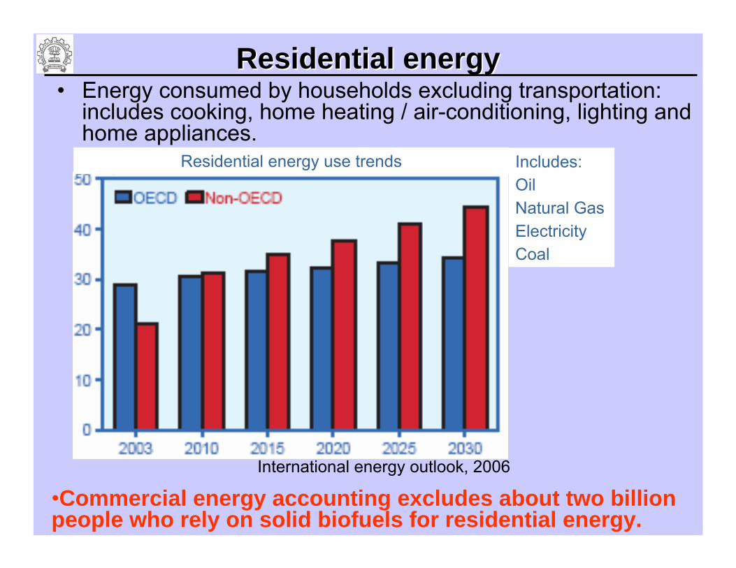
• Energy consumed by households excluding transportation: includes cooking, home heating / air-conditioning, lighting and home appliances.

Residential energy Residential energy

•Commercial energy accounting excludes about two billion people who rely on solid biofuels for residential energy.

International energy outlook, 2006

Residential energy use trends Includes:OilNatural GasElectricityCoal

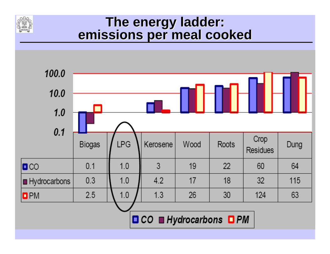
The energy ladder: The energy ladder: emissions per meal cookedemissions per meal cooked

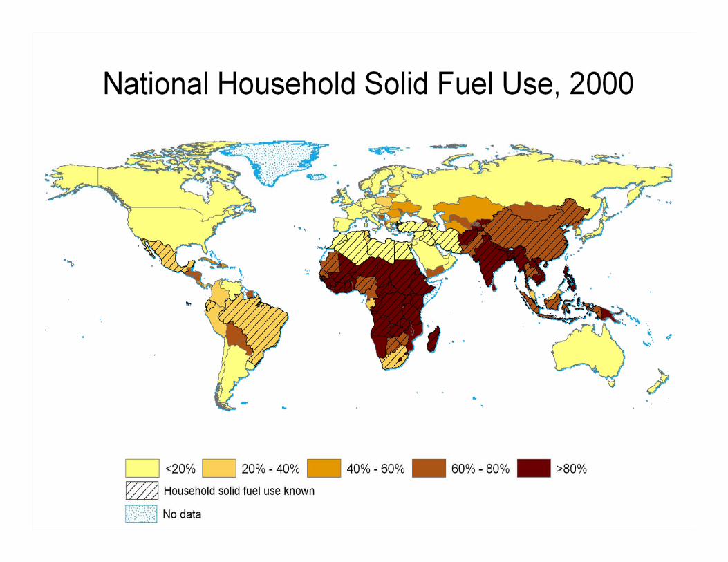
National Household Use of Biomass and Coal in 2000

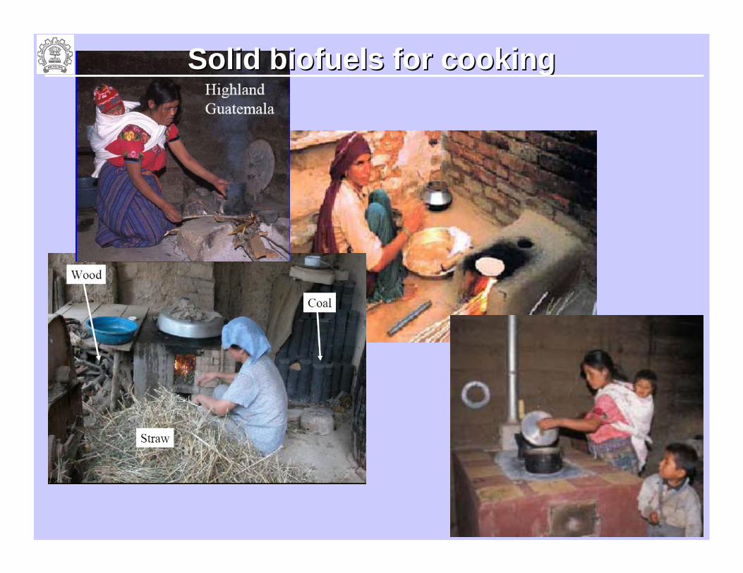
Solid Solid biofuelsbiofuels for cookingfor cooking

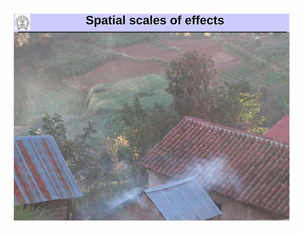
Spatial scales of effectsSpatial scales of effects

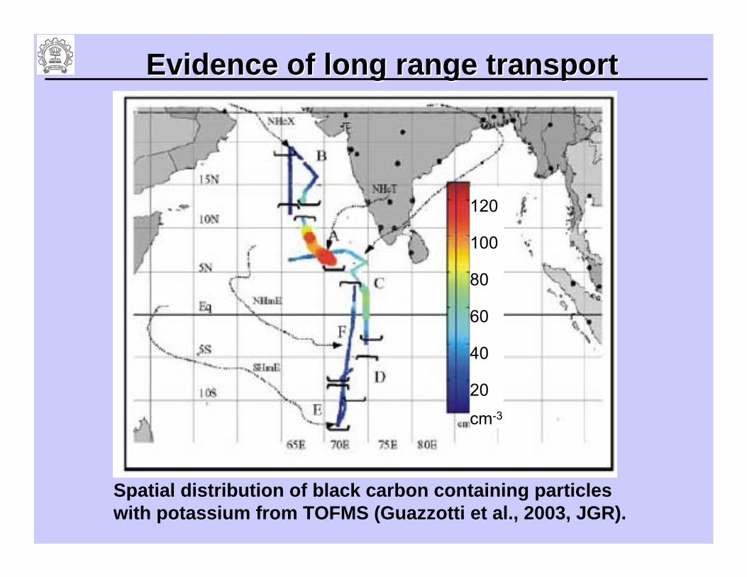
Evidence of long range transportEvidence of long range transport

120

100

80

60

40

20

cm-3

Spatial distribution of black carbon containing particles with potassium from TOFMS (Guazzotti et al., 2003, JGR).

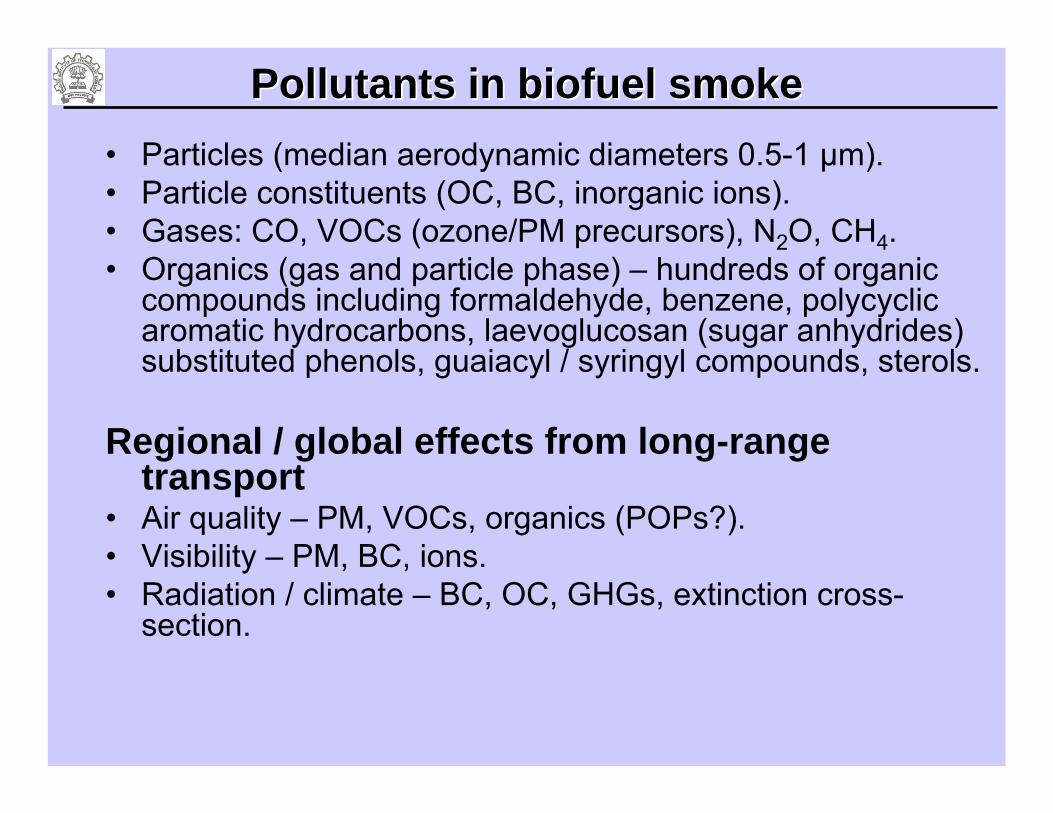
• Particles (median aerodynamic diameters 0.5-1 μm).• Particle constituents (OC, BC, inorganic ions).• Gases: CO, VOCs (ozone/PM precursors), N2O, CH4.• Organics (gas and particle phase) – hundreds of organic

compounds including formaldehyde, benzene, polycyclic aromatic hydrocarbons, laevoglucosan (sugar anhydrides) substituted phenols, guaiacyl / syringyl compounds, sterols.

Regional / global effects from long-range transport

• Air quality – PM, VOCs, organics (POPs?).• Visibility – PM, BC, ions.• Radiation / climate – BC, OC, GHGs, extinction cross-

section.

Pollutants in Pollutants in biofuelbiofuel smokesmoke

Emissions inventory methodologyEmissions inventory methodology• Activity levels (usually fuels) (kg day-1)

Per capita usage, user population, fuel-mix.

• Technology divisionsDevices, efficiency (thermal and combustion).

• Emission factors (g kg-1)Pollutants of interest for each fuel-technology system.

• Spatial distribution and resolutionAppropriate proxy – typically population.

• Temporal resolution and seasonal cycleFoods / fuels may vary with season.

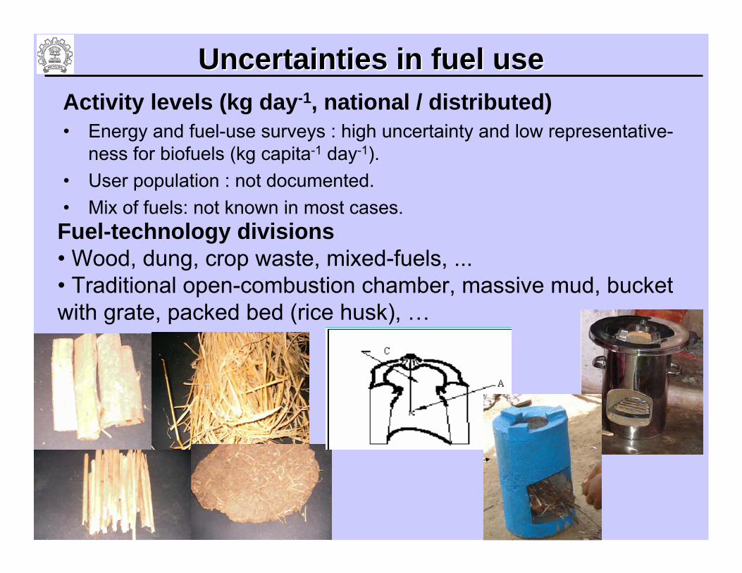
Activity levels (kg day-1, national / distributed)• Energy and fuel-use surveys : high uncertainty and low representative-

ness for biofuels (kg capita-1 day-1).• User population : not documented. • Mix of fuels: not known in most cases.

Uncertainties in fuel useUncertainties in fuel use

Fuel-technology divisions • Wood, dung, crop waste, mixed-fuels, ...• Traditional open-combustion chamber, massive mud, bucket with grate, packed bed (rice husk), …

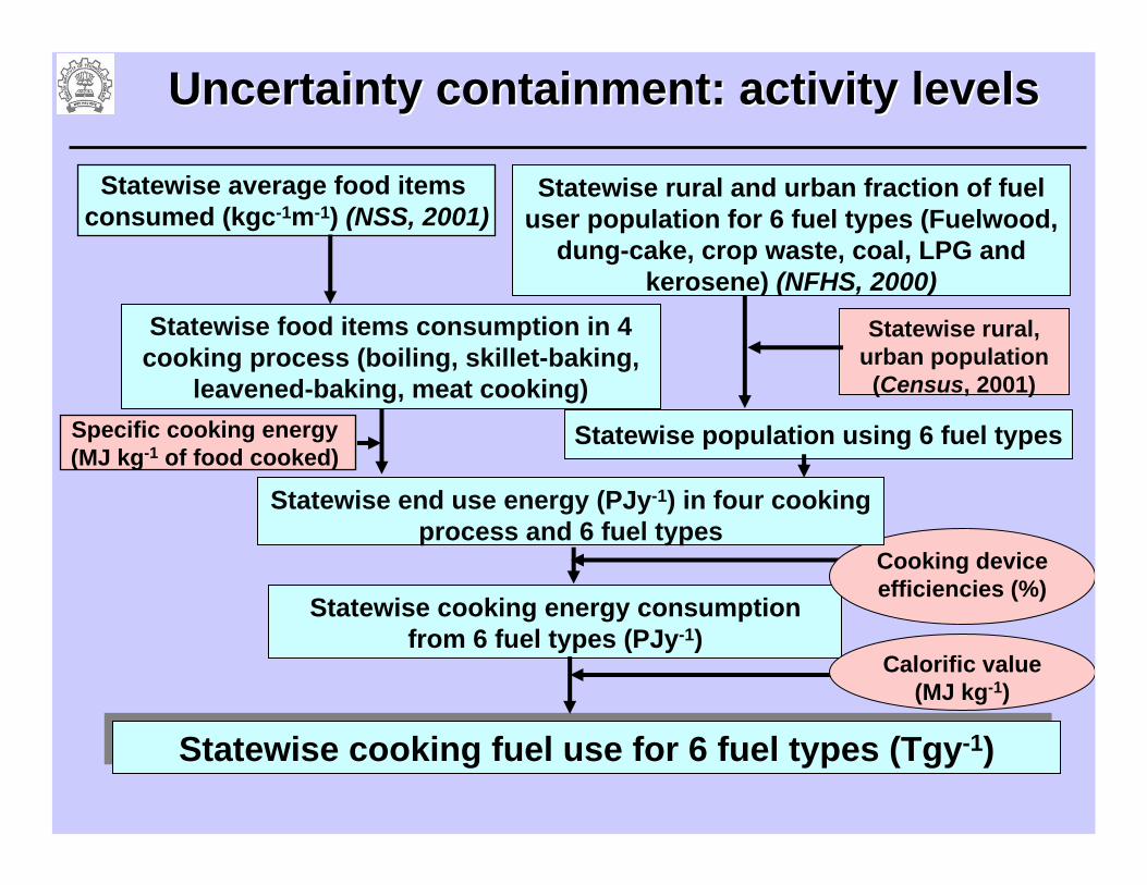
Statewise cooking energy consumption from 6 fuel types (PJy-1)

Specific cooking energy (MJ kg-1 of food cooked)

Statewise cooking fuel use for 6 fuel types (Tgy-1)Statewise cooking fuel use for 6 fuel types (Tgy-1)

Statewise average food items consumed (kgc-1m-1) (NSS, 2001)

Cooking device efficiencies (%)

Calorific value (MJ kg-1)

Statewise rural and urban fraction of fuel user population for 6 fuel types (Fuelwood,

dung-cake, crop waste, coal, LPG and kerosene) (NFHS, 2000)

Statewise population using 6 fuel types

Statewise rural, urban population (Census, 2001)

Statewise end use energy (PJy-1) in four cooking process and 6 fuel types

Statewise food items consumption in 4 cooking process (boiling, skillet-baking,

leavened-baking, meat cooking)

Uncertainty containment: activity levelsUncertainty containment: activity levels

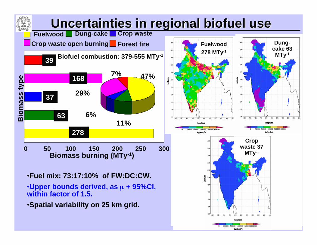
Uncertainties in regional Uncertainties in regional biofuelbiofuel useuseFuelwood Dung-cake Crop waste

Crop waste open burning Forest fire

0 50 100 150 200 250 300

278

63

37

168

39

6%11%

47%

29%

7%

0 50 100 150 200 250 300Biomass burning (MTy-1)

Bio

mas

s ty

pe

Biofuel combustion: 379-555 MTy-1

Biofuels379 MTy-1

•Fuel mix: 73:17:10% of FW:DC:CW. •Upper bounds derived, as μ + 95%CI, within factor of 1.5.•Spatial variability on 25 km grid.

Fuelwood278 MTy-1

Dung-cake 63 MTy-1

Crop waste 37

MTy-1

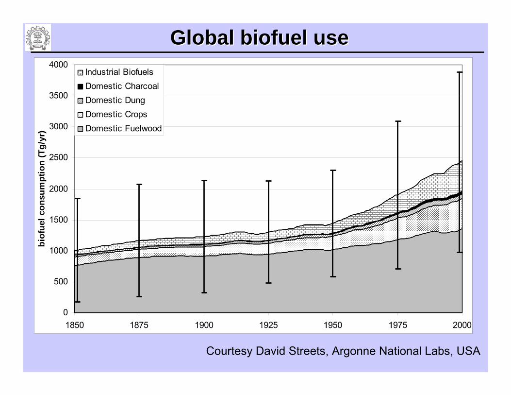
Global Global biofuelbiofuel useuse

0

500

1000

1500

2000

2500

3000

3500

4000

1850 1875 1900 1925 1950 1975 2000

biof

uel c

onsu

mpt

ion

(Tg/

yr)

Industrial BiofuelsDomestic CharcoalDomestic DungDomestic CropsDomestic Fuelwood

Courtesy David Streets, Argonne National Labs, USA

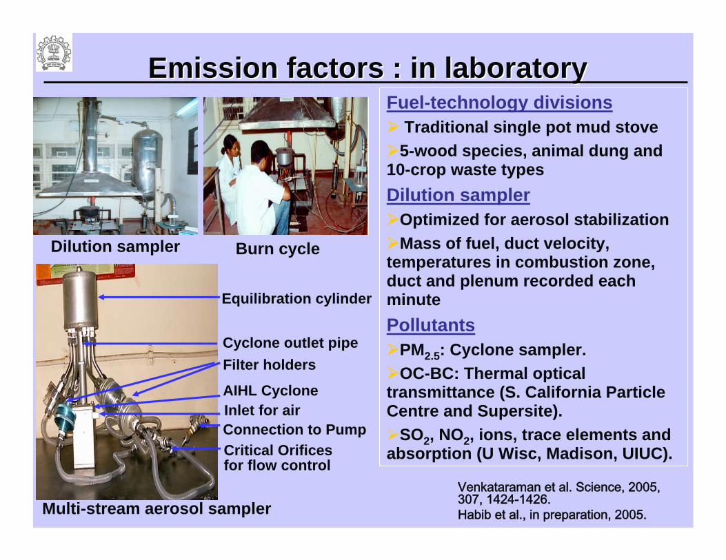
Emission factors : in laboratoryEmission factors : in laboratoryFuel-technology divisions

Traditional single pot mud stove5-wood species, animal dung and

10-crop waste typesDilution sampler

Optimized for aerosol stabilizationMass of fuel, duct velocity,

temperatures in combustion zone, duct and plenum recorded each minutePollutants

PM2.5: Cyclone sampler.OC-BC: Thermal optical

transmittance (S. California Particle Centre and Supersite).

SO2, NO2, ions, trace elements and absorption (U Wisc, Madison, UIUC).

Dilution sampler Burn cycle

Multi-stream aerosol sampler

AIHL Cyclone

Equilibration cylinder

Inlet for air

Filter holders Cyclone outlet pipe

Connection to PumpCritical Orifices for flow control

Venkataraman et al. Science, 2005, 307, 1424-1426. Habib et al., in preparation, 2005.

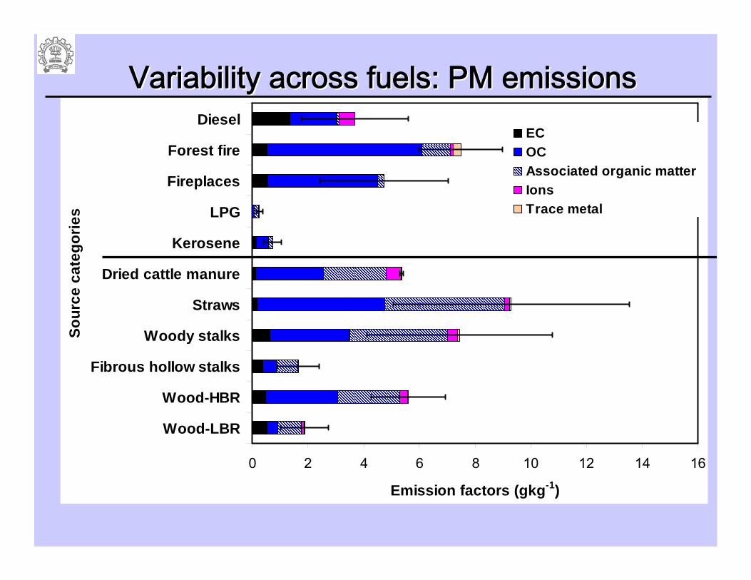
Variability across fuels: PM emissionsVariability across fuels: PM emissions

0 2 4 6 8 10 12 14 16

Wood-LBR

Wood-HBR

Fibrous hollow stalks

Woody stalks

Straws

Dried cattle manure

Kerosene

LPG

Fireplaces

Forest fire

Diesel

Sour

ce c

ateg

orie

s

Emission factors (gkg-1)

ECOCAssociated organic matterIonsTrace metal

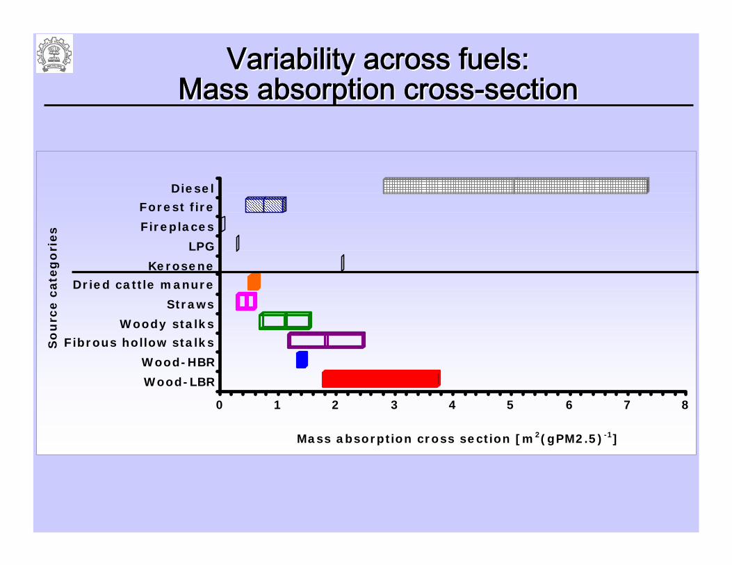
Variability across fuels: Variability across fuels: Mass absorption crossMass absorption cross--sectionsection

0 1 2 3 4 5 6 7 8

Mass absorption cross section [m2(gPM2.5)-1]

Wood-LBR

Wood-HBR

Fibrous hollow stalks

Woody stalks

Straws

Dried cattle manure

Kerosene

LPG

Fireplaces

Forest fire

Diesel

So

urc

e c

ate

go

ries

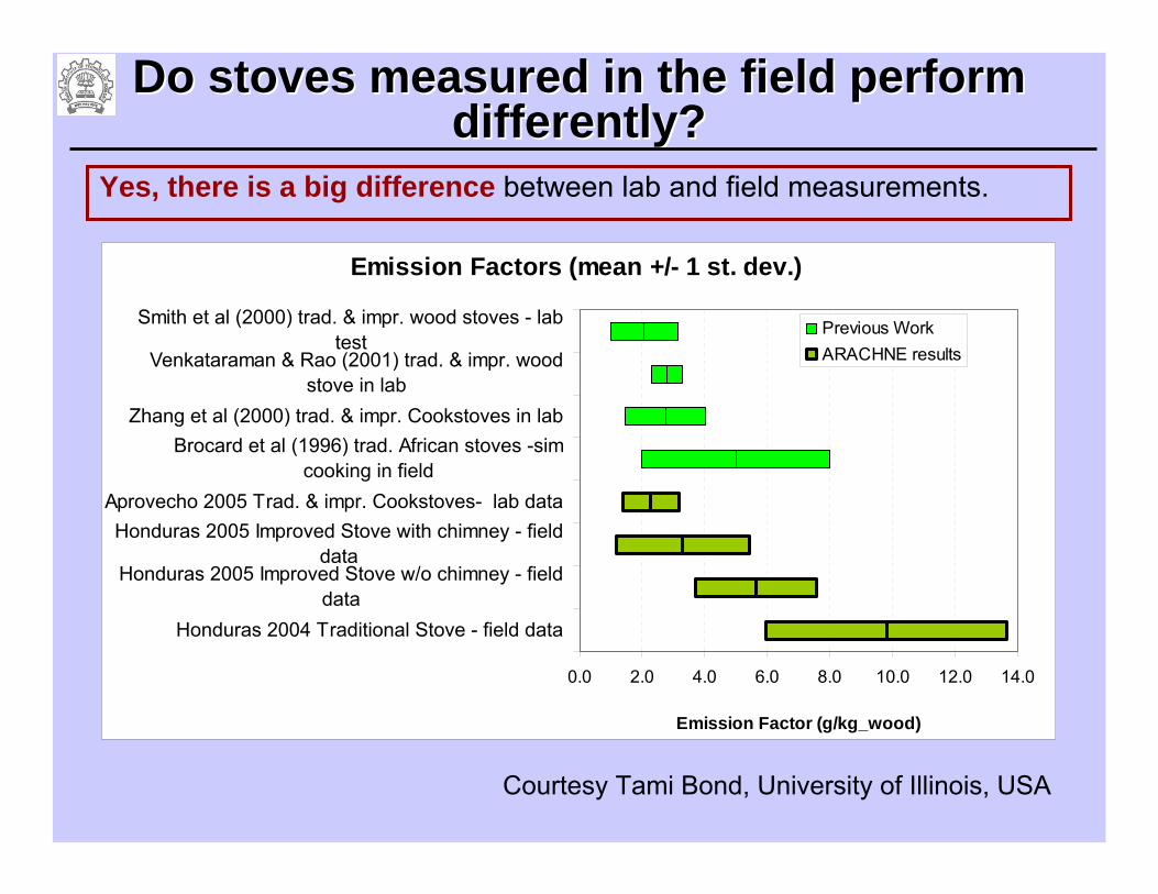
Do stoves measured in the field perform Do stoves measured in the field perform differently?differently?

Emission Factors (mean +/- 1 st. dev.)

0.0 2.0 4.0 6.0 8.0 10.0 12.0 14.0

Honduras 2004 Traditional Stove - field data

Honduras 2005 Improved Stove w/o chimney - fielddata

Honduras 2005 Improved Stove with chimney - fielddata

Aprovecho 2005 Trad. & impr. Cookstoves- lab data

Brocard et al (1996) trad. African stoves -simcooking in field

Zhang et al (2000) trad. & impr. Cookstoves in lab

Venkataraman & Rao (2001) trad. & impr. woodstove in lab

Smith et al (2000) trad. & impr. wood stoves - labtest

Emission Factor (g/kg_wood)

Previous WorkARACHNE results

Yes, there is a big difference between lab and field measurements.

Courtesy Tami Bond, University of Illinois, USA

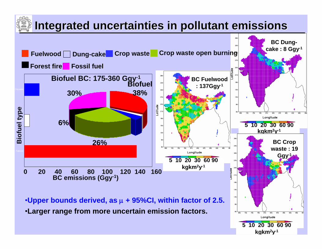
Integrated uncertainties in pollutant emissionsIntegrated uncertainties in pollutant emissions

BC Fuelwood: 137Ggy-1

BC Dung-cake : 8 Ggy-1

5 10 20 30 60 90kgkm2y-1

5 10 20 30 60 90kgkm2y-1

BC Crop waste : 19

Ggy-1

5 10 20 30 60 90kgkm2y-1

Fuelwood Dung-cake Crop waste

Fossil fuelForest fire

Crop waste open burning

0 20 40 60 80 100 120 140 160

Fuelwood

Dung-cake

Crop waste

BC emissions (Ggy-1)

Bio

fuel

type

Biofuel38%

6%

0 20 40 60 80 100 120 140 160

Biofuel BC: 175-360 Ggy-1

30%

26%

•Upper bounds derived, as μ + 95%CI, within factor of 2.5.•Larger range from more uncertain emission factors.

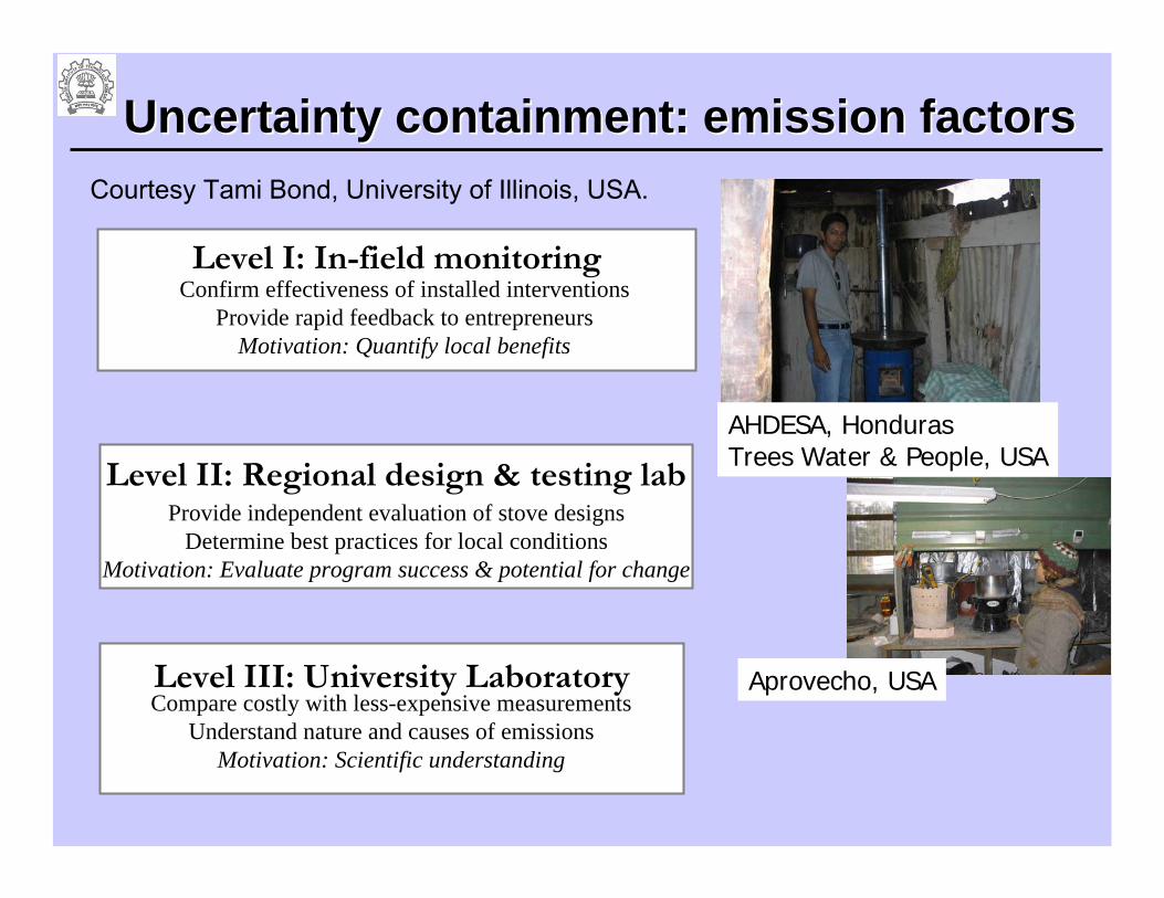
Level I: In-field monitoring

Level II: Regional design & testing lab

Confirm effectiveness of installed interventionsProvide rapid feedback to entrepreneurs

Motivation: Quantify local benefits

Provide independent evaluation of stove designsDetermine best practices for local conditions

Motivation: Evaluate program success & potential for change

Level III: University LaboratoryCompare costly with less-expensive measurements

Understand nature and causes of emissionsMotivation: Scientific understanding

AHDESA, HondurasTrees Water & People, USA

Aprovecho, USA

Uncertainty containment: emission factorsUncertainty containment: emission factorsCourtesy Tami Bond, University of Illinois, USA.

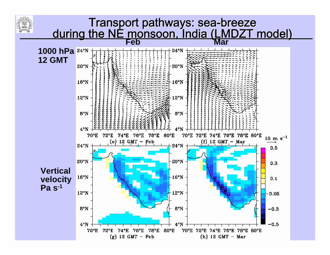
Transport pathways: seaTransport pathways: sea--breeze breeze during the NE monsoon, India (LMDZT model)during the NE monsoon, India (LMDZT model)

1000 hPa12 GMT

Feb Mar

Vertical velocityPa s-1

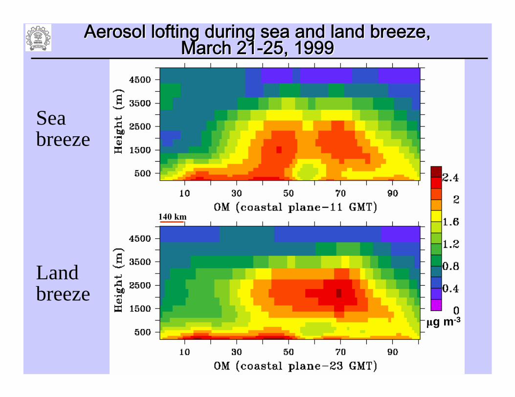
Aerosol lofting during sea and land breeze, Aerosol lofting during sea and land breeze, March 21March 21--25, 199925, 1999

Sea breeze

Landbreeze

μg m-3

140 km

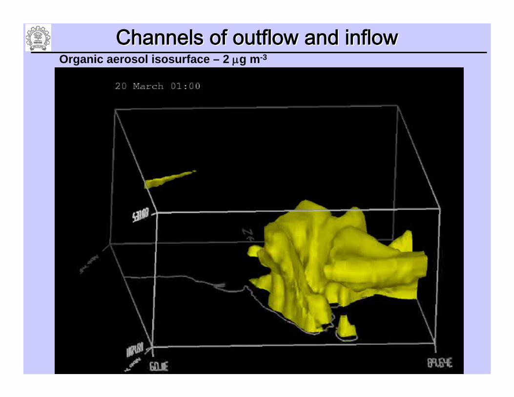
Channels of outflow and inflowChannels of outflow and inflowOrganic aerosol isosurface – 2 μg m-3

ModellingModelling with region tagged emissionswith region tagged emissions

AFWAAFWA

ROWROW

EAEA

SEASEA

SISI

CNICNI

NWINWI

IGPIGP

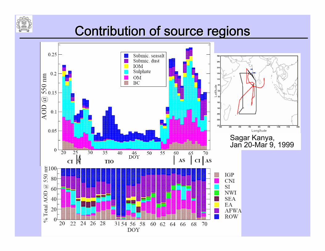
Sagar Kanya, Jan 20-Mar 9, 1999

Contribution of source regionsContribution of source regions

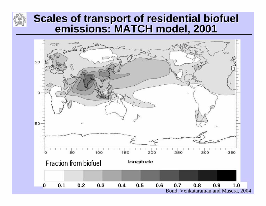
Fraction from biofuelFraction from biofuel

0 0.1 0.2 0.3 0.4 0.5 0.6 0.7 0.8 0.9 1.0Bond, Venkataraman and Masera, 2004

Scales of transport of residential Scales of transport of residential biofuelbiofuelemissions: MATCH model, 2001emissions: MATCH model, 2001

Question: how much of indoor biofuel smoke penetrates to the outside?

• Need local measurements of simultaneous indoor / outdoor concentrations.

• Local-scale grid model and / or receptor model to estimate indoor source contribution to the outdoors.

Local / regional air quality linkage to HTAPLocal / regional air quality linkage to HTAP

Current InventoriesCurrent InventoriesGeographical and temporal resolution for modellingHTAP:- Regional inventories show spatial features at 25 km resolution (e.g Habib et al., 2004; Venkataraman et al., 2005). Global would need resolution at or finer than wind fields used in driving models (100-200 km?).

-Monthly mean temporal resolution to capture seasonal variations in food-fuels, and space heating needs.

-Regional inventories (Streets et al, 2003; Habib et al., 2004; Venkataraman et al., 2005) can be nested / merged with global ones (e.g. Bond et al., 2004 for BC). Compatible in uncertainties.

-Upcoming global biofuel trends inventory (Streets et al., 2006)indicates need for long-term accounting.

Inventory improvementInventory improvement• Global activity database linked to survey data

(stove, fuel, food).- Food consumption statistics and measurements cooking energy may be more robust than fuel use surveys.

• Emission factors - Need to reconcile lab and field measurements.- Need University-NGO collaboration to make statistically valid measurement datasets of emissions.- Need to leverage health study networks to make local-global link.- Need simple automated field instruments that can be widely deployed.