Calculus of Variations

Valeriy Slastikov & Georgy Kitavtsev Spring, 2017

1 1D Calculus of Variations.

We are going to study the following general problem:

• Minimize functional

I(u) =

∫ b

af(x, u(x), u′(x)) dx

subject to boundary conditions u(a) = α, u(b) = β.

In order to correctly set up this problem we have to assume certain properties of f(x, u, ξ) and afunction u(x). Since we know how to integrate continuous functions it is reasonable to assume thatfunction f : [a, b]×R×R→ R is continuous. In fact in this section we will need stronger assumptionthat f ∈ C2([a, b]× R× R), meaning that f , f ′ and f ′′ are continuous functions.

Concerning function u : [a, b] → R we may assume that u ∈ C1([a, b]) and u(a) = α, u(b) = β.It seems reasonable since minimization problem involves u′(x) (that needs to be continuous since weknow how to integrate continuous functions) and boundary conditions. In fact in this section we willuse a bit stronger regularity assumption u ∈ C2([a, b]).

Note: we can change boundary conditions by removing constraints at one or both ends. In general,one can not prescribe u′ at the end points (this will be explained later).

We are ready to set up the problem with mathematical precision:Define

I(u) ≡∫ b

af(x, u(x), u′(x)) dx, (1)

where f ∈ C2([a, b]× R× R), u ∈ C1([a, b]).

Problem:infu∈X

I(u), (2)

where X = {u ∈ C1([a, b]) : u(a) = α, u(b) = β}.

We want to find a function u0(x) such that u0 ∈ X and u0 delivers minimum to the functional I(u)(we call such function a minimizer). In order to do this we need to understand what it means tominimize the functional I(u).

Definition 1.1 Function u0 ∈ X is a minimizer (or global minimizer) of the functional I(u) on a setX if

I(u0) ≤ I(u) for all u ∈ X.

Definition 1.2 Function u0 ∈ X is a local minimizer of the functional I(u) if the following holds forsome open set N 3 u0

I(u0) ≤ I(u) for all u ∈ N ⊂ X.

1

In general it is very difficult to solve (2), however one can try to characterize minimizers. Let’sconsider a simple example from Calculus.

Example 1.1 Let g ∈ C1([a, b]) and we want to find a minimizer of g. By well known result ofAnalysis we know that any continuous function on a compact interval (closed and bounded) achievesits minimum (and maximum). Obviously the minimizer is just some point x0 ∈ [a, b]. In order to findit we have to use the definition, i.e.

g(x0) ≤ g(x) for all x ∈ [a, b].

Assume that x0 ∈ (a, b) then for any x ∈ (a, b) we have

f(x)− f(x0)

x− x0≥ 0, if x > x0

andf(x)− f(x0)

x− x0≤ 0, if x < x0.

Taking a limit x→ x0 we obtain f ′(x0) ≥ 0 and f ′(x0) ≤ 0. Therefore we have f ′(x0) = 0. Note: wemust assume x0 ∈ (a, b) in order to obtain f ′(x0) = 0, explain it.In order to find a minimizer we must find all points where f ′(x) = 0 and compare values at thesepoints with values at the ends of the interval (f(a), f(b)).

In order to characterize minimizers of I(u) we proceed in the similar way. We know that if u0 is aminimizer then I(u0) ≤ I(u) for all u ∈ X. Take any function h ∈ C1

0 ([a, b]), obviously u0 + th ∈ Xand therefore

I(u0) ≤ I(u0 + th) for all h ∈ C10 ([a, b]).

We can define a function F (t) = I(u0 + th) and notice that since u0 is a minimizer of I(u) then t = 0is a minimizer of F (t) on R. Therefore we must have F ′(0) = 0 (see example).Note: we a priori assumed existence of minimizer u0 ∈ X for I(u) and just trying to characterize

it if it exists. In the example above for 1D function existence was guaranteed by a simple result ofAnalysis (look it up).

We characterize minimizers in the following theorem

Theorem 1.3 Let f ∈ C2([a, b]× R× R) (f ≡ f(x, u, ξ)) and

infu∈X

{I(u) ≡

∫ b

af(x, u(x), u′(x)) dx

}= m, (3)

where X = {u ∈ C1([a, b]) : u(a) = α, u(b) = β}. Then

1. If (3) admits a minimizer u0 ∈ X ∩ C2([a, b]) then

d

dx

(fξ(x, u0(x), u′0(x))

)= fu(x, u0(x), u′0(x)) x ∈ (a, b) (4)

u0(a) = α, u0(b) = β.

2. If some function u∗ ∈ X∩C2([a, b]) satisfies (4) and if (u, ξ)→ f(x, u, ξ) is convex (as a functionof two variables) for every x ∈ [a, b] then u∗ is a minimizer of (3).

2

Proof. 1) As we discussed before, if u0 ∈ X is a minimizer of I(u) then F ′(0) = 0 (see the definitionof F above). Let’s find F ′(0): by definition of derivative

F ′(0) = limt→0

F (t)− F (0)

t= lim

t→0

I(u0 + th)− I(u0)

t.

It’s not difficult to see that

I(u0 + th)− I(u0)

t=

∫ b

a

f(x, u0(x) + th(x), u′0(x) + th′(x))− f(x, u0(x), u′0(x))

tdx. (5)

Passing to the limit and using standard Analysis results to interchange integral and limit (for instanceDominated Convergence Theorem) we obtain

F ′(0) =

∫ b

a

d

dtf(x, u0(x) + th(x), u′0(x) + th′(x))

∣∣t=0

dx.

Using standard rules of differentiation we have

d

dtf(x, u0(x) + th(x), u′0(x) + th′(x))

∣∣t=0

= fu(x, u0(x), u′0(x))h(x) + fξ(x, u0(x), u′0(x))h′(x). (6)

Therefore if u0 ∈ X is a minimizer of I(u) we must have∫ b

afu(x, u0(x), u′0(x))h(x) + fξ(x, u0(x), u′0(x))h′(x) dx = 0

for all h ∈ C10 ([a, b]). This is a weak form of Euler-Lagrange equation. It is not clear how to deal with

this integral identity and therefore we want to obtain a pointwise identity. We can use integration byparts to obtain∫ b

afξ(x, u0(x), u′0(x))h′(x) dx

= −∫ b

a

d

dx

(fξ(x, u0(x), u′0(x))

)h(x) dx+ fξ(x, u0(x), u′0(x))h(x)

∣∣ba. (7)

Recalling that h(a) = h(b) = 0 we have∫ b

a

[fu(x, u0(x), u′0(x))− d

dx

(fξ(x, u0(x), u′0(x))

)]h(x) dx = 0

for all h ∈ C10 ([a, b]). Using Fundamental Lemma of Calculus of Variations (proved after this theorem)

we obtain

fu(x, u0(x), u′0(x))− d

dx

(fξ(x, u0(x), u′0(x))

)= 0 x ∈ (a, b).

Conditions u0(a) = α, u0(b) = β follow from the fact u0 ∈ X.

2) Let u∗ ∈ X ∩ C2([a, b]) is a solution of (4). Since f(x, u, ξ) is convex in last two variables we have

f(x, u(x), u′(x)) ≥ f(x, u∗(x), u′∗(x)) + fu(x, u∗(x), u′∗(x))(u(x)− u∗(x))

+ fξ(x, u∗(x), u′∗(x))(u′(x)− u′∗(x)) (8)

3

for every u ∈ X (this inequality will be shown later for a convex function of one variable, extend it).We can integrate both parts of this inequality over (a, b) to obtain∫ b

af(x, u(x), u′(x)) dx ≥

∫ b

af(x, u∗(x), u′∗(x)) dx+

∫ b

afu(x, u∗(x), u′∗(x))(u(x)− u∗(x)) dx

+

∫ b

afξ(x, u∗(x), u′∗(x))(u′(x)− u′∗(x)) dx. (9)

Using integration by parts and noting that u− u∗ ∈ C10 ([a, b]) we obtain

I(u) ≥ I(u∗) +

∫ b

a

[fu(x, u∗(x), u′∗(x))− d

dx

(fξ(x, u∗(x), u′∗(x))

)](u(x)− u∗(x)) dx. (10)

Since u∗ satisfies (4) we have I(u) ≤ I(u∗) for all u ∈ X.Theorem is proved.

Remark. Note that we did not prove existence of minimizer in this theorem. In the first statementwe showed that if u0 is a minimizer then it solves Euler-Lagrange equation. In the second statementwe showed that if u∗ solves Euler-Lagrange equation and the function f is convex in last twovariables then u∗ is a minimizer. But we did not prove existence of solution for Euler-Lagrangeequation and therefore even the case of convex f we don’t know if there is a minimizer.

Now we prove Fundamental Lemma of Calculus of Variations (FLCV)

Lemma 1.1 Let g ∈ C([a, b]) and∫ b

ag(x)η(x) dx = 0 for all η ∈ C∞0 ([a, b]),

then g(x) = 0 on [a, b].

Proof. Suppose there exists a point c ∈ (a, b) such that g(c) 6= 0. We may assume without loss ofgenerality that g(c) > 0. By continuity of function g(x) there exists an open interval (s, t) ⊂ (a, b)containing point c such that g(x) > 0 on (s, t). Taking η(x) to be positive on (s, t) with η(s) = η(t) = 0

we obtain the contradiction with∫ ba g(x)η(x) dx = 0. Therefore g(x) = 0 for all x ∈ (a, b). By

continuity of g we obtain g(x) = 0 on [a, b].Lemma is proved.

For convenience we also prove a simple fact that for g ∈ C1([a, b]) convexity is equivalent to

g(x) ≥ g(y) + g′(y)(x− y) for all x, y ∈ (a, b).

Proof. Let g be convex then by definition

g(αx+ (1− α)y) ≤ αg(x) + (1− α)g(y)

for all α ∈ (0, 1) and x, y in (a, b). After simple rearrangement we have

g(y + α(x− y))− g(y)

α≤ g(x)− g(y).

4

Taking a limit as α→ 0 we obtain

g′(y)(x− y) ≤ g(x)− g(y).

We proved it in one direction. Now we assume

g(x) ≥ g(y) + g′(y)(x− y) for all x, y ∈ (a, b).

Using this we have

g(x) ≥ g(αx+ (1− α)y) + (1− α)g′(αx+ (1− α)y)(x− y)

andg(y) ≥ g(αx+ (1− α)y)− αg′(αx+ (1− α)y)(x− y).

Multiplying first inequality by α, second inequality by 1− α and adding them we obtain

αg(x) + (1− α)g(y) ≥ g(αx+ (1− α)y).

Result is proved.

Note that this fact is true also for functions defined on Rn.

Let’s consider several examples.

Example 1.2 (Brachistochrone problem) In this example we have

f(u, ξ) =

√1 + ξ2

u,

and X = {u ∈ C1([0, 1]) : u(0) = 0, u(1) = β, u(x) > 0 for x ∈ (0, 1) }. We would like to findsolutions of Euler-Lagrange equation.

Using theorem 1.3 we can easily find Euler-Lagrange equations(u′√

u[1 + (u′)2]

)′= −

√1 + (u′)2

4u3.

We can multiply both parts by u′√u[1+(u′)2]

and obtain

(u′√

u[1 + (u′)2]

)′u′√

u[1 + (u′)2]= − u′

2u2.

It is clear that this is equivalent to ((u′)2

u[1 + (u′)2]

)′=

(1

u

)′.

Now we obtain1

u=

(u′)2

u[1 + (u′)2]+ C

5

and simplifying this expression we obtain

u[1 + (u′)2] = 2µ,

where µ > 0 is some constant that we can find from boundary conditions. Separating variables weobtain

dx =

√u

2µ− udu.

Now we integrate both parts

x =

∫ u

0

√y

2µ− ydy.

We can make a natural substitution y = µ(1− cos θ) to obtain x = µ(θ− sin θ). Therefore solution tothis problem can be represented in the following parametric form:

u(θ) = µ(1− cos θ), x(θ) = µ(θ − sin θ).

It is clear that u(0) = 0 so that first boundary condition is satisfied and we can find µ by applyingsecond boundary condition.Note that we don’t know if this solution is a minimizer of the problem. For this we have to proveeither existence of minimizer or convexity of f(u, ξ). However from physical model we can see thatthere must be a solution here (therefore minimizer should exist) and since solution to the problem isunique it must be a minimizer (I guess that was the reasoning in 17-th century).

Example 1.3 (Minimal surface of revolution) In this example we have

f(u, ξ) = 2πu√

1 + ξ2,

and X = {u ∈ C1([0, 1]) : u(0) = α, u(1) = β, u(x) > 0 }. We would like to find solutions ofEuler-Lagrange equation.

Again we can use the theorem 1.3 to obtain(uu′√

1 + (u′)2

)′=√

1 + (u′)2.

Multiplying both parts by uu′√1+(u′)2

and integrating we obtain

u2

1 + (u′)2= C, or (u′)2 =

u2

a2− 1

for some constant a > 0. We can separate variables to obtain the solution here but there is a betterway: we search for a solution in the following form

u(x) = a coshf(x)

a.

Plugging this into equation we obtain [f ′(x)]2 = 1 and therefore either f(x) = x+µ or f(x) = −x+µ.Since coshx is even function and µ is any constant we have

u(x) = a coshx+ µ

a.

Continue to find the solutions of this problem assuming u(0) = u(1) = α > 0. The number of solutionswill depend on α.

6

Example 1.4 (Convexity) In this example we assume that f(ξ) is convex on R and X = {u ∈C1([a, b]) : u(a) = α, u(b) = β, }. We will prove existence of minimizer for

I(u) =

∫ b

af(u′(x)) dx

in this case and find it explicitly. By convexity of f we know that

f(x) ≥ f(y) + f ′(y)(x− y).

We can define u0(x) = β−αb−a (x− a) + α. Using above inequality we see that for any u ∈ X

f(u′(x)) ≥ f(u′0(x)) + f ′(u′0(x))(u′(x)− u′0(x)).

It is clear that u′0(x) ≡ β−αb−a and therefore integrating both parts over (a, b) we obtain∫ b

af(u′(x)) dx ≥

∫ b

af(u′0(x)) dx.

Therefore u0 is a minimizer of I(u).

Now we give several examples of nonexistence.

Example 1.5 (Non-convexity implies no minimizer) We consider f(ξ) = e−ξ2

and X = {u ∈C1([0, 1]) : u(0) = 0, u(1) = 0, } and want to show that for the problem

infX

∫ 1

0f(u′(x)) dx

there is no solution.We see that Euler-Lagrange equation is

d

dxf ′(u′) = 0.

And therefore u′ = const that implies in this case (using boundary conditions) that u(x) ≡ 0. It isclear that this is a maximizer of the problem, not a minimizer. Moreover, if we take

un(x) = n(x− 1

2)2 − n

4

we have un ∈ X for any n ∈ N. Calculating I(un) we obtain

I(un) =

∫ 1

0e−4n

2(x− 12)

2

dx =1

2n

∫ n

−ne−x

2dx→ 0,

as n → ∞. Therefore infX I(u) = 0 but obviously no function can deliver this infimum and sominimizer does not exist.

Example 1.6 (Not smooth minimizers) Consider f(ξ) = (ξ2−1)2 , X = {u ∈ C1([0, 1]) : u(0) =0, u(1) = 0, }. Show that there are no minimizers for this problem. However there are infinitely manyminimizers that are piecewise smooth.

7

1.1 Problems with constraints - Lagrange multipliers

In many problems arising in applications there exist some integral constraints on the set of functionswhere we look for a minimizer. One basic example is Catenary problem where we have to find theshape of the hanging chain of fixed length (see example below). In order to characterize the minimizerof the problem (2) with integral constraint

G(u) ≡∫ b

ag(x, u(x), u′(x)) dx = 0 (11)

we can not simply take a variation of the functional I(u) with respect to any function h ∈ C10 ([a, b])

since we can violate this integral constraint. Therefore we have to invent a method that allowsus to derive Euler-Lagrange equation in this situation. This method is called Method of LagrangeMultipliers. Let’s state the problem that we are solving here with mathematical precision.

We investigate minimizers of the following problem

infu∈Y

∫ b

af(x, u(x), u′(x)) dx, (12)

where

Y = X ∩ {u ∈ C1([a, b]) : G(u) ≡∫ b

ag(x, u(x), u′(x)) dx = 0}.

We can prove the following theorem

Theorem 1.4 Let f, g ∈ C2([a, b]×R×R) and u0 be a minimizer of the problem (12) above such that∫ b

agξ(x, u0(x), u′0(x))w′(x) + gu(x, u0(x), u′0(x))w(x) dx 6= 0 (13)

for some w ∈ C10 ([a, b]). Then u0 satisfies Euler-Lagrange equations corresponding to the following

probleminf

(u,λ)∈X×RI(u)− λG(u). (14)

Proof. Let u0 be a minimizer of (12). We would like to take a variation o I(u) preserving constraintG(u) = 0. By (13) (rescaling if needed) we know that there exists a function w ∈ C1

0 ([a, b]) such that∫ b

agξ(x, u0(x), u′0(x))w′(x) + gu(x, u0(x), u′0(x))w(x) dx = 1. (15)

Let v ∈ C10 ([a, b]) be any and w be as above, we define eeewsddq4

F (ε, h) = I(u0 + εv + hw) =

∫ b

af(x, u0(x) + εv(x) + hw(x), u′0(x) + εv′(x) + hw′(x)) dx (16)

and

G(ε, h) = G(u0 + εv + hw) =

∫ b

ag(x, u0(x) + εv(x) + hw(x), u′0(x) + εv′(x) + hw′(x)) dx. (17)

8

We know that G(0, 0) = G(u0) = 0 (since u0 satisfies constraint (11)) and Gh(0, 0) = 1 (since u0satisfies (15)). Using Implicit Function Theorem we can deduce that there exists ε0 and a continuouslydifferentiable function t(ε) such that t(0) = 0 and

G(ε, t(ε)) = 0

for all ε ∈ [−ε0, ε0]. Therefore we know that for all ε ∈ [−ε0, ε0] we have

u0 + εv + t(ε)w ∈ Y.

Now we can take a variation of I(u). We consider F (ε, t(ε)) = I(u0 + εv + t(ε)w), by the samearguments as before since u0 is a minimizer of I(u) and since F (0, 0) = I(u0) we know that 0 is aminimizer of function F (ε, t(ε)) and therefore

d

dεF (ε, t(ε))

∣∣ε=0

= 0.

Computing this derivative we obtain

Fε(0, 0) + Fh(0, 0)t′(0) = 0.

It’s not difficult to see that

Fh(0, 0) =

∫ b

afξ(x, u0(x), u′0(x))w′(x) + fu(x, u0(x), u′0(x))w(x) dx,

and since u0 and w are fixed functions Fh(0, 0) is just a constant that we denote as λ ≡ Fh(0, 0). Wehave to understand what is t′(0) and in order to do this we use the fact that G(ε, t(ε)) = 0 for allε ∈ [−ε0, ε0] and compute

0 =d

dεG(ε, t(ε))

∣∣ε=0

= Gε(0, 0) +Gh(0, 0)t′(0).

Since Gh(0, 0) = 1 then t′(0) = −Gε(0, 0). Therefore we have that if u0 is a minimizer of I(u) then

Fε(0, 0)− λGε(0, 0) = 0.

We may rewrite this as∫ b

afu(x, u0(x), u′0(x))v(x) + fξ(x, u0(x), u′0(x))v′(x) dx−

λ

∫ b

agξ(x, u0(x), u′0(x))v′(x) + gu(x, u0(x), u′0(x))v(x) dx = 0 (18)

for all v ∈ C10 ([a, b]). Using integration by parts, FLCV and recalling that G(u0) = 0 we obtain

d

dx

(fξ(x, u0(x), u′0(x))

)− fu(x, u0(x), u′0(x))

= λ

(d

dx

(gξ(x, u0(x), u′0(x))

)− gu(x, u0(x), u′0(x))

)x ∈ (a, b) (19)

∫ b

ag(x, u0(x), u′0(x)) dx = 0

This is exactly Euler-Lagrange equation for the problem (14).Theorem is proved.

9

Remark. Think about why we need condition with w.

Example 1.7 (Catenary problem) Solve this problem.

10

2 Second Variation and Stability

In the previous section we introduced a minimization problem and learned a method to find criticalpoints of the functional I(u) using Euler-Lagrange equations. However we still don’t know anythingabout how to solve the original minimization problem. In particular we don’t understand if the criticalpoints that we find by solving Euler-Lagrange equations are minimisers or not, i.e. if they ”stable” or”unstable” (in a certain sense). This section is devoted to investigating stability of the critical pointof I(u) using its second variation.

2.1 Various Derivatives

In this section we start with introduction for the functional (1) an analog of Taylor expansion (for afunction of two variables) and subsequently of two different notions of functional derivatives, namelyGateaux and Frechet.

Let us assume that f ∈ C3([a, b] × R̄ × R̄) (in particular, its third order partial derivativesfuuu, fuuξ, fuξξ, fξξξ are continuous and bounded functions on [a, b] × R × R) and recall Peano’sform of it’s Taylor expansion at a point (x, u, ξ):

f(x, u+ φ, ξ + h) = f(x, u, ξ) + (fuφ+ fξh) +1

2(fuuφ

2 + 2fuhφh+ fξξh2)

+1

6(f̄uuuφ

3 + 3f̄uuhφ2h+ 3f̄uhhφh

2 + f̄ξξξh3). (20)

In the last expression derivatives without bars are evaluated at the point (x, u, ξ), and derivatives withbars are evaluated at an intermediate point (x, u+ θ1φ, ξ + θ2h) for some numbers 0 ≤ θ1, θ2 ≤ 1.

Substitution of expansion (20) into the functional I(u) in (1) and taking

ξ(x) = u′(x), h(x) = φ′(x) for x ∈ [a, b] with φ(a) = φ(b) = 0

results in the following expansion of functional I(u) at point u:

I(u+ φ)− I(u) =

∫ b

afuφ+ fξφ

′ dx+1

2

∫ b

afuuφ

2 + 2fuξφφ′ + fξξ|φ′|2 dx

+1

6

∫ b

a(f̄uuuφ

3 + 3f̄uuhφ2φ′ + 3f̄uhhϕ|φ′|2 + f̄ξξξ(φ

′)3) dx

=: δI(u)[φ] +1

2δ2I(u)[φ] +R(u, φ), (21)

Above we have introduced three new functionals, which depend on point u:

δI(u)[φ] :=

∫ b

afuφ+ fξφ

′ dx,

δ2I(u)[φ] :=

∫ b

a(fuuφ

2 + 2fuξφφ′ + fξξ|φ′|2) dx,

R(u, φ) :=1

6

∫ b

a(f̄uuuφ

3 + 3f̄uuhφ2φ′ + 3f̄uhhφ|φ′|2 + f̄ξξξ(φ

′)3) dx. (22)

11

Next, it is easy to get the following estimates:

|δ2I(u)[φ]| ≤ 1

2M

∫ b

a(φ2 + 2|φφ′|+ φ′2) dx =

1

2M

∫ b

a(|φ|+ |φ′|)2 dx

≤ b− a2

M ||φ||2C1[a,b], (23)

where M := max{fuu, fuξ, fξξ} in [a, b] × R × R (by assumptions on f the maximum exists) and asusually

||φ||C1[a,b] := maxx∈[a,b]

(|φ(x)|+ |φ′(x)|

).

Analogously, it can be shown that

|R(u, φ)| ≤ b− a3

M1||φ||3C1[a,b], (24)

where M1 := max{fuuu, fuuξ, fuξξ, fξξξ} in [a, b]× R× R.Using expansion (21) of the functional I(u) we can give a meaning to the following definition.

Definition 2.1 Let u ∈ C1([a, b]), φ ∈ C10 ([a, b]) and I : C1([a, b]) → R be a functional (see for

instance (1)). We say that I is Frechet differentiable at u if there exists a linear functional δIF (u) :C10 ([a, b])→ R (called a first Frechet variation/derivative of I(u) at the point u) such that

lim‖φ‖C1([a,b])→0

|I(u+ φ)− I(u)− δIF (u)[φ]|‖φ‖C1([a,b])

= 0.

If the above limit exists for all u ∈ C1([a, b]), we say that I is Frechet differentiable in C1([a, b]).

Note that in the above definition you can change C1([a, b]) and R to any Banach spaces X, Y . Note,that expansion (21) and estimates (23)–(24) imply together for functional (1) that its Frechet derivativeδI(u)[φ] is indeed given by the first formula in (22).

Analogously, we introduce a definition of the second variation as follows.

Definition 2.2 Functional F (φ, h) is called to be bilinear on C1[a, b] × C1[a, b]) if F (·, h) is linearfunctional of φ for any fixed h ∈ C1[a, b]) and also F (φ, ·) is linear functional of h for any fixedφ ∈ C1[a, b]). Given a bilinear functional F (φ, h) we can always define a quadratic functional E[φ] bya restriction:

E(φ) := F (φ, φ), for all φ ∈ C1[a, b].

Note that according to the last definition functional δ2I(u)[φ] in (22) is quadratic with the correspond-ing bilinear functional F (u) given by

F (u)[φ, h] =

∫ b

a(fuuφh+ 2fuξφφ

′ + fξξφh) dx.

Definition 2.3 Let u ∈ C1([a, b]), φ ∈ C10 ([a, b]) and I : C1([a, b]) → R be a functional (see for

instance (1)). We say that I is twice Frechet differentiable at u if there exists δI(u) : C1([a, b])→ Rfrom Definition 2.1 and a quadratic functional δ2I(u) : C1

0 ([a, b]) → R (called as second Frechetvariation/derivative of I(u) at the point u) such that

lim‖φ‖C1([a,b])→0

|I(u+ φ)− I(u)− δIF (u)[φ]− 12δ

2IF (u)[φ]|‖φ‖2

C10 ([a,b])

= 0.

If the above limit exists for all u ∈ C1([a, b]) we say that I is twice Frechet differentiable in C1([a, b]).

12

Again expansion (21) and estimate (24) imply together for functional (1) that thus defined δ2I(u)[φ]is indeed given by the second formula in (22).

We end this section with introducing an alternative definition of the first and second variationswhich are easier to use in practice.

Definition 2.4 Let u ∈ C1([a, b]), φ ∈ C10 ([a, b]) and I : C1([a, b]) → R be a functional (see for

instance (1)). We define Gateaux derivative of I at the point u in the direction φ as

δIG(u)[φ] = limt→0

I(u+ tφ)− I(u)

t.

If the above limit exists for all φ ∈ C10 ([a, b]) we say that I is Gateaux differentiable in C1([a, b]).

We already implicitly used Gateaux derivative in the previous section when we were taking firstvariation of the functional I(u).

Definition 2.5 Assuming f ∈ C2 we define the second Gateaux variation of I at the point u ∈C1([a, b]) in the direction φ ∈ C1

0 ([a, b]) as

δ2IG(u)(φ) =d2

dt2∣∣∣t=0

I(u+ tφ).

Replacement of φ by tφ in the expansion (21) and differentiation with respect to t (once or twice)along with the subsequent limit t → 0 give again the formulas for δI(u)[φ] and δ2I(u)[φ] stated in(22). Therefore, we may conclude with the following statement.

Proposition 2.6 Let f ∈ C3([a, b]× R̄× R̄) then the first and the second variations of functional (1)in the sense of Gateaux and Frechet coincide and are given by

δI(u)[φ] :=

∫ b

afuφ+ fξφ

′ dx, (25)

δ2I(u)[φ] :=

∫ b

a(fuuφ

2 + 2fuξφφ′ + fξξ|φ′|2) dx. (26)

Remark. Note that there is a difference between Gateaux and Frechet derivatives. In fact it’s clearthat existence of Frechet derivative implies existence of Gateaux derivative. The opposite, in general,is not true. We explain it in the next section.

2.2 Examples showing difference between Frechet and Gateaux derivatives

Definitions of Frechet and Gateaux derivatives can be easily transferred to the case of functions oftwo variables f : R×R→ R, in which case Frechet derivative coincides with the full differential of f ,while Gateaux derivative coincides with derivatives in the direction of vector ν̄ ∈ R. In this case weknow from Analysis course that:

Existence of Frechet derivative =⇒ Existence of Gateaux derivative =⇒ Existence of partial derivatives.

The following examples show that inverse implications are not true.

13

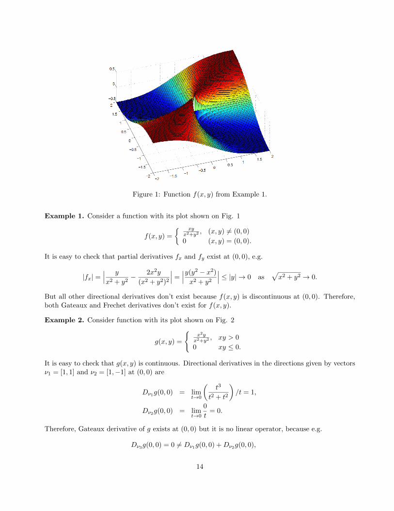
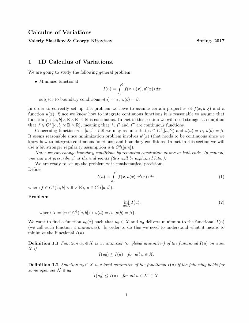
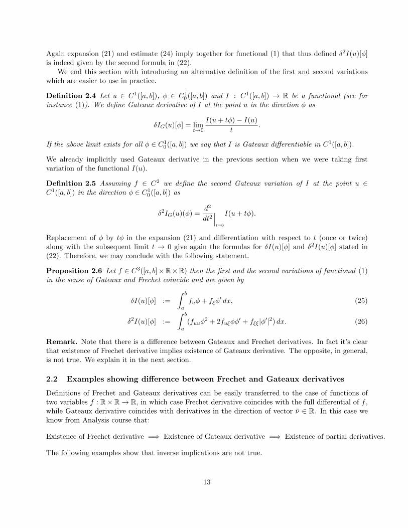
Figure 1: Function f(x, y) from Example 1.

Example 1. Consider a function with its plot shown on Fig. 1

f(x, y) =

{ xyx2+y2

, (x, y) 6= (0, 0)

0 (x, y) = (0, 0).

It is easy to check that partial derivatives fx and fy exist at (0, 0), e.g.

|fx| =∣∣∣ y

x2 + y2− 2x2y

(x2 + y2)2

∣∣∣ =∣∣∣y(y2 − x2)x2 + y2

∣∣∣ ≤ |y| → 0 as√x2 + y2 → 0.

But all other directional derivatives don’t exist because f(x, y) is discontinuous at (0, 0). Therefore,both Gateaux and Frechet derivatives don’t exist for f(x, y).

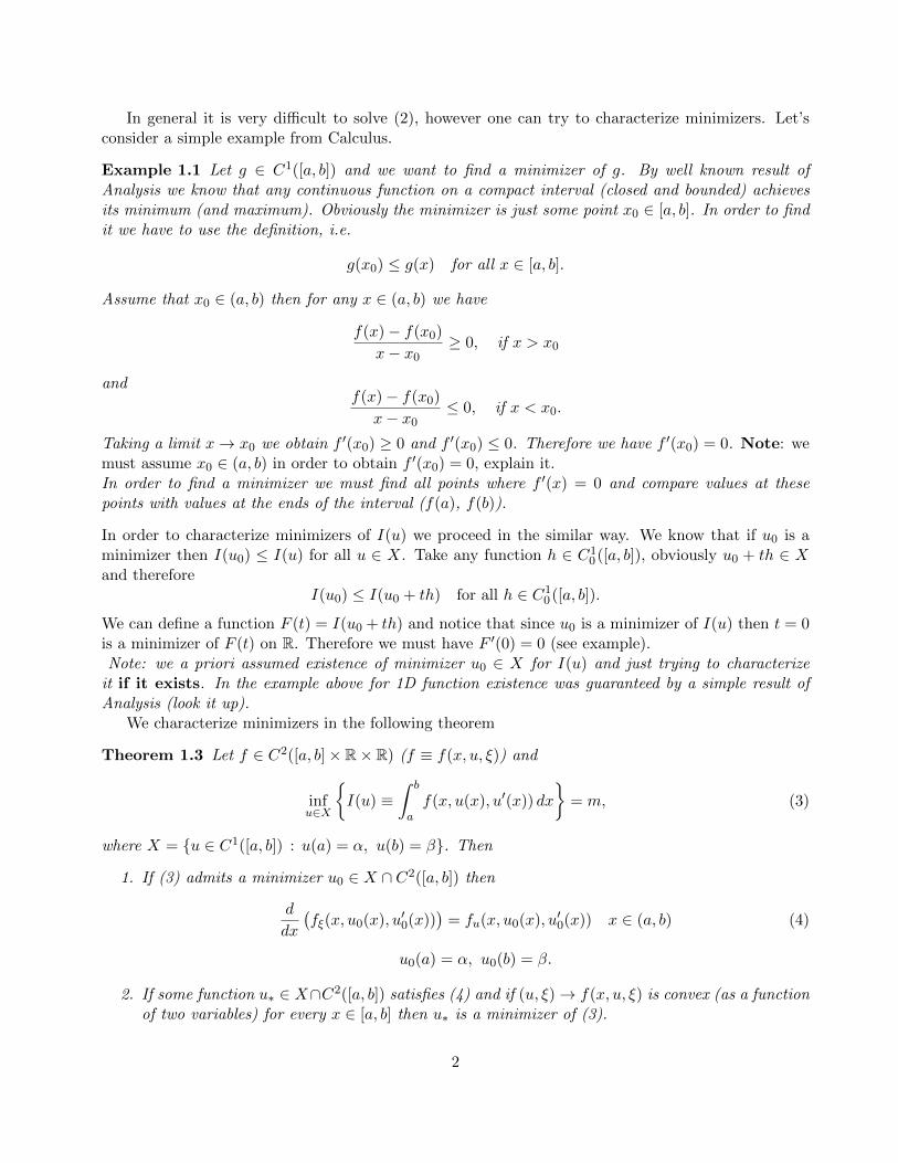
Example 2. Consider function with its plot shown on Fig. 2

g(x, y) =

{x2yx2+y2

, xy > 0

0 xy ≤ 0.

It is easy to check that g(x, y) is continuous. Directional derivatives in the directions given by vectorsν1 = [1, 1] and ν2 = [1,−1] at (0, 0) are

Dν1g(0, 0) = limt→0

(t3

t2 + t2

)/t = 1,

Dν2g(0, 0) = limt→0

0

t= 0.

Therefore, Gateaux derivative of g exists at (0, 0) but it is no linear operator, because e.g.

Dν3g(0, 0) = 0 6= Dν1g(0, 0) +Dν2g(0, 0),

14

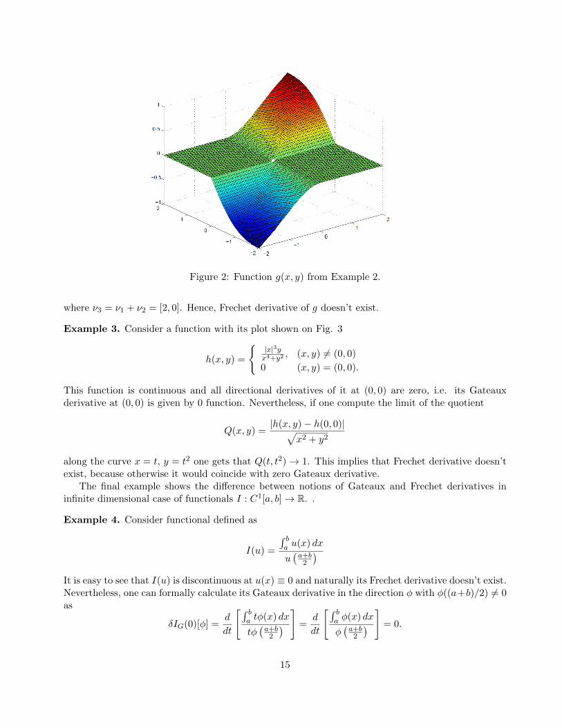
Figure 2: Function g(x, y) from Example 2.

where ν3 = ν1 + ν2 = [2, 0]. Hence, Frechet derivative of g doesn’t exist.

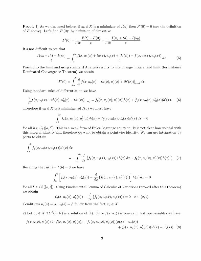
Example 3. Consider a function with its plot shown on Fig. 3

h(x, y) =

{|x|3yx4+y2

, (x, y) 6= (0, 0)

0 (x, y) = (0, 0).

This function is continuous and all directional derivatives of it at (0, 0) are zero, i.e. its Gateauxderivative at (0, 0) is given by 0 function. Nevertheless, if one compute the limit of the quotient

Q(x, y) =|h(x, y)− h(0, 0)|√

x2 + y2

along the curve x = t, y = t2 one gets that Q(t, t2)→ 1. This implies that Frechet derivative doesn’texist, because otherwise it would coincide with zero Gateaux derivative.

The final example shows the difference between notions of Gateaux and Frechet derivatives ininfinite dimensional case of functionals I : C1[a, b]→ R. .

Example 4. Consider functional defined as

I(u) =

∫ ba u(x) dx

u(a+b2

)It is easy to see that I(u) is discontinuous at u(x) ≡ 0 and naturally its Frechet derivative doesn’t exist.Nevertheless, one can formally calculate its Gateaux derivative in the direction φ with φ((a+b)/2) 6= 0as

δIG(0)[φ] =d

dt

[∫ ba tφ(x) dx

tφ(a+b2

) ] =d

dt

[∫ ba φ(x) dx

φ(a+b2

) ] = 0.

15

Figure 3: Function h(x, y) from Example 3.

2.3 Computing Second Variation

Now we are ready to compute the second variation of the functional

I(u) =

∫ b

af(x, u(x), u′(x)) dx

defined on X = {u ∈ C1([a, b]), u(a) = α, u(b) = β} directly using Definition 2.5.

δ2I(u)(φ) =

∫ b

a

(φ2fuu(x, u, u′) + 2φφ′fuξ(x, u, u

′) + |φ′|2fξξ)dx.

We can integrate this expression by parts taking into account φ ∈ C10 ([a, b]) to obtain

δ2I(u)(φ) =

∫ b

a

(φ2[fuu(x, u, u′)− d

dxfuξ(x, u, u

′)

]+ |φ′|2fξξ

)dx.

The second variation is extremely important in the investigation of the stability and local minimalityof the critical point of functional I(u).

2.4 Second Variation and Stability

We know that if f R→ R is twice differentiable function and x0 is a critical point of f then f ′(x0) = 0.If we want to understand more about nature of x0, i.e. if it is local minimum, local maximum or asaddle point we know from basic analysis that we have to investigate the sign of f ′′(x0). In particular

• if f ′′(x0) > 0 then x0 is local minimum, i.e. there exists δ > 0 such that f(x0) ≤ f(x) for allx ∈ (x0 − δ, x0 + δ) ;

• if f ′′(x0) < 0 then x0 is local maximum, i.e. there exists δ > 0 such that f(x0) ≥ f(x) for allx ∈ (x0 − δ, x0 + δ) ;

16

• if f ′′(x0) = 0 then nothing definite can be said about properties of x0 and in order to concludeyou need to consider higher order derivatives.

Remark. Recall that we used analogy between 1D problems and infinite dimensional problem in theprevious section when finding necessary conditions on the criticality of u0. Think about how you canprove above statements using convexity (concavity) of f or Taylor expansion of f near x0. Can youtransfer your ideas to the infinite dimensional case?

We are interested in minimization problem and therefore we want to single out local minimizers(if we cannot find global minimizer). We already understand that local minimizers of I(u) have tosatisfy Euler-Lagrange equations. Now we want to show that local minimizers have to satisfy morerestrictive condition.

Proposition 2.7 Let u0 ∈ X = {u ∈ C1([a, b]), u(a) = α, u(b) = β} be a local minimizer of thefunctional I(u) defined in (1), i.e. there exists δ > 0 such that I(u0) ≤ I(u) for all u ∈ X such that‖u− u0‖C1 < δ. Then

δ2I(u0)(φ) ≥ 0 for all φ ∈ C10 ([a, b]). (27)

Proof Assume that there is φ0 ∈ C10 ([a, b]) such that δ2I(u0)(φ0) < 0. Define function F (t) =

I(u0 + tφ0). It’s clear that t = 0 is a critical point of F (t) and F ′(0) = 0, F ′′(0) < 0. Now you canuse 1D arguments to show that there exists δ > 0 such that F (0) > F (t) for all t ∈ (t− δ, t+ δ), t 6= 0and this is in contradiction with local minimality of u0.

Based on this result we introduce several definitions

Definition 2.8 The critical point u0 ∈ X of the functional I(u) is called locally stable if δ2I(u0)(φ) ≥0 for all φ ∈ C∞0 ([a, b]); strictly locally stable if δ2I(u0)(φ) > 0 for all φ ∈ C∞0 ([a, b]); and uniformlylocally stable in space Y if δ2I(u0)(φ) > µ‖φ‖2Y for all φ ∈ C∞0 ([a, b]).

Remark. Here space Y does not necessarily coincides with X and usually is much weaker than Y .The typical example for Y in our framework would be either W 1,p

0 (a, b) or Lp(a, b) for some p > 1. Ingeneral, there is no hope to take Y = C1

0 ([a, b]) and prove uniform positivity of the second variationfor I. That’s why you need to study Sobolev and Lp spaces if you want to do research in Calculus ofVariations.

There is another necessary condition (Legendre condition) for local stability that directly follows fromdefinition of local stability.

Proposition 2.9 Let I(u) be defined as usually (see (1)), u0 is a critical point of I(u) and δ2I(u0)(φ) ≥0 for all φ ∈ C∞0 ([a, b]) then

fξξ(x, u0(x), u′0(x)) ≥ 0 for all x ∈ [a, b].

Proof Proof is a simple exercise. Try to use a mollifier in the neighborhood of a point x to show thatfξξ(x, u0(x), u′0(x)) ≥ 0.

17

2.5 Local Minimality

In the previous section we introduced the notion of local stability. However, in order to show localminimality it is in general not enough to have local stability.

Definition 2.10 We say that u0 ∈ X is a local minimizer of I(u) if there exists δ > 0 such thatI(u0) ≤ I(u) for all u ∈ X such that ‖u− u0‖X < δ.

Next example shows that condition (27) is not sufficient for a critical point to be a minimizer.

Example 1. Define a functional

I(u) =

∫ 1

0u3 dx.

u(x) ≡ 0 is a critical point of this functional and

δ2I(0)[φ] = 0, for all φ ∈ C10 ([a, b],

but u(x) is not a local minimizer. Hint for the proof: calculate the reminder term R(0, φ) in theexpansion (21)-(22) and show that it is negative when φ(x) < 0. In fact, I(u) doesn’t have a minimizerand for a sequence un ≡ −n one has

I(un)→ −∞.

Next example shows that in contrast to the case of functions of several variables condition

δ2I(u)(φ) > 0, for all φ ∈ C10 ([a, b],

is still not sufficient for a critical point u to be a local minimizer of functional I.

Example 2. Define a functional

I(u) =

∫ 1

0

(2

3u3 − x2u2

)dx.

It is easy to show that u(x) = x2 is a critical point of this functional and

δ2I(u)[φ] = 2

∫ 1

0x2φ2 dx > 0 for φ 6= 0 (28)

We can also calculate the reminder term in the expansion (21)-(22) as

R(u, φ) = 4

∫ 1

0φ3 dx (29)

Let us take a sequence of functions {φn} defined as (see also Fig. 4):

φn(x) =

−xn , 0 ≤ x ≤ 1

2n1n(x− 1

n) 12n < x ≤ 1

n0 1

n < x ≤ 1.

Substituting {φn} into the formulas (28) and (29) gives

R(u, φn) = − 1

8n7and δ2I(u)(φ) =

11

240n7.

18

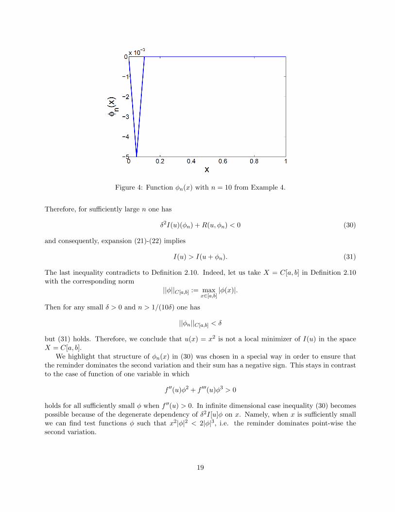
Figure 4: Function φn(x) with n = 10 from Example 4.

Therefore, for sufficiently large n one has

δ2I(u)(φn) +R(u, φn) < 0 (30)

and consequently, expansion (21)-(22) implies

I(u) > I(u+ φn). (31)

The last inequality contradicts to Definition 2.10. Indeed, let us take X = C[a, b] in Definition 2.10with the corresponding norm

||φ||C[a,b] := maxx∈[a,b]

|φ(x)|.

Then for any small δ > 0 and n > 1/(10δ) one has

||φn||C[a,b] < δ

but (31) holds. Therefore, we conclude that u(x) = x2 is not a local minimizer of I(u) in the spaceX = C[a, b].

We highlight that structure of φn(x) in (30) was chosen in a special way in order to ensure thatthe reminder dominates the second variation and their sum has a negative sign. This stays in contrastto the case of function of one variable in which

f ′′(u)φ2 + f ′′′(u)φ3 > 0

holds for all sufficiently small φ when f ′′(u) > 0. In infinite dimensional case inequality (30) becomespossible because of the degenerate dependency of δ2I[u]φ on x. Namely, when x is sufficiently smallwe can find test functions φ such that x2|φ|2 < 2|φ|3, i.e. the reminder dominates point-wise thesecond variation.

19

Proposition 2.11 Uniform local stability implies local minimality and, therefore, the former is indeeda sufficient condition.

Proof The proof uses again the expansion (21)-(22). In order to satisfy Definition 2.10 we takeδ = 3µ/(2M1(b− a)), where M1 is as in estimate (24) for the reminder. Then for all φ such that

||φ||C10 [a,b]

< δ and φ 6= 0

one can estimateI(u+ φ)− I(u) = δ2I(u)[φ]−R(u, φ) >

µ

2||φ||C1

0 [a,b]> 0

and hence u is a local minimiser.

3 Important Examples

In this section we study several important examples that shows how to obtain the information on thesecond variation and how to use it to show local (and sometimes global) minimality.

Example 1. Let’s define I(u) in the following way

I(u) =

∫ R

0

(1

2|u′|2 +

1

4(u2 − 1)2

)dx.

We define set X = {u ∈ C1([0, R]), u(0) = 0, u(R) = 1} and want to solve the following problem

infu∈X

I(u).

At this point we know that in order to find a solution to this problem we have to find critical pointsby solving Euler-Lagrange equations. There is no guarantee that what we find is a minimizer but wewill try to investigate its stability later.

Euler-Lagrange equations

It is clear that Euler-Lagrange equations are

u′′ = u(u2 − 1), u(0) = 0, u(R) = 1.

If you want to find the solution here you can reduce this equation to a first order equation that youmight be able to solve. Multiplying both parts of the above equation by u′ and integrating from 0 tox we obtain ∫ R

x

1

2

(|u′(s)|2

)′ds =

∫ R

x

1

4

((u2(s)− 1)2

)′ds

This gives us the following relation

1

2|u′(R)|2 − 1

2|u′(x)|2 =

1

4

((u2(R)− 1)2

)− 1

4

((u2(x)− 1)2

).

20

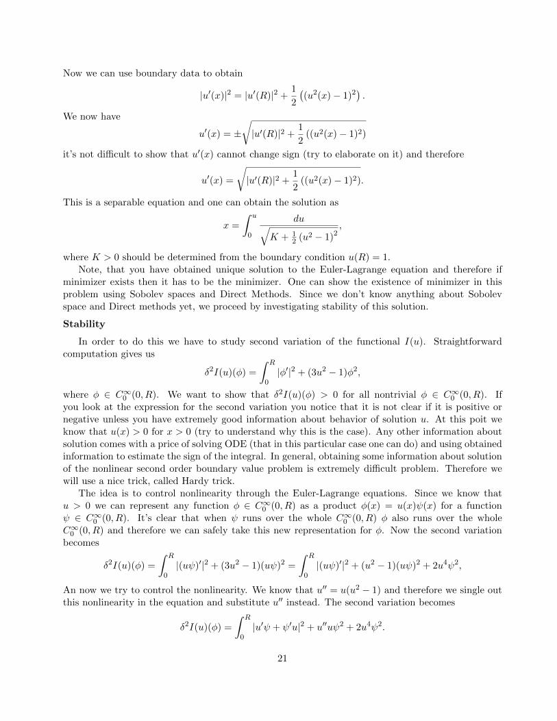
Now we can use boundary data to obtain

|u′(x)|2 = |u′(R)|2 +1

2

((u2(x)− 1)2

).

We now have

u′(x) = ±√|u′(R)|2 +

1

2((u2(x)− 1)2)

it’s not difficult to show that u′(x) cannot change sign (try to elaborate on it) and therefore

u′(x) =

√|u′(R)|2 +

1

2((u2(x)− 1)2).

This is a separable equation and one can obtain the solution as

x =

∫ u

0

du√K + 1

2 (u2 − 1)2,

where K > 0 should be determined from the boundary condition u(R) = 1.Note, that you have obtained unique solution to the Euler-Lagrange equation and therefore if

minimizer exists then it has to be the minimizer. One can show the existence of minimizer in thisproblem using Sobolev spaces and Direct Methods. Since we don’t know anything about Sobolevspace and Direct methods yet, we proceed by investigating stability of this solution.

Stability

In order to do this we have to study second variation of the functional I(u). Straightforwardcomputation gives us

δ2I(u)(φ) =

∫ R

0|φ′|2 + (3u2 − 1)φ2,

where φ ∈ C∞0 (0, R). We want to show that δ2I(u)(φ) > 0 for all nontrivial φ ∈ C∞0 (0, R). Ifyou look at the expression for the second variation you notice that it is not clear if it is positive ornegative unless you have extremely good information about behavior of solution u. At this poit weknow that u(x) > 0 for x > 0 (try to understand why this is the case). Any other information aboutsolution comes with a price of solving ODE (that in this particular case one can do) and using obtainedinformation to estimate the sign of the integral. In general, obtaining some information about solutionof the nonlinear second order boundary value problem is extremely difficult problem. Therefore wewill use a nice trick, called Hardy trick.

The idea is to control nonlinearity through the Euler-Lagrange equations. Since we know thatu > 0 we can represent any function φ ∈ C∞0 (0, R) as a product φ(x) = u(x)ψ(x) for a functionψ ∈ C∞0 (0, R). It’s clear that when ψ runs over the whole C∞0 (0, R) φ also runs over the wholeC∞0 (0, R) and therefore we can safely take this new representation for φ. Now the second variationbecomes

δ2I(u)(φ) =

∫ R

0|(uψ)′|2 + (3u2 − 1)(uψ)2 =

∫ R

0|(uψ)′|2 + (u2 − 1)(uψ)2 + 2u4ψ2,

An now we try to control the nonlinearity. We know that u′′ = u(u2 − 1) and therefore we single outthis nonlinearity in the equation and substitute u′′ instead. The second variation becomes

δ2I(u)(φ) =

∫ R

0|u′ψ + ψ′u|2 + u′′uψ2 + 2u4ψ2.

21

After integrating by parts second term and basic algebra we obtain

δ2I(u)(φ) =

∫ R

0|u′|2ψ2 + |ψ′|2u2 + 2u′uψ′ψ − |u′|2ψ2 − 2u′uψ′ψ + 2u4ψ2 (32)

=

∫ R

0|ψ′|2u2 + 2u4ψ2 > 0. (33)

We have shown that second variation is strictly positive. Therefore we proved that u is strictly locallystable. Now we want to investigate local minimality. In general, to investigate local minimality onehas to show uniform local stability in some space. However in this particular case we will be able toprove evenglobal minimality of u by direct calculation.

Global minimality

Let’s take two energies I(v) and I(u), where u is our critical point and v ∈ X is any function. Wewant to show that I(v) > I(u). We first show that I(u+ φ)− I(u) > 0 for any φ ∈ C∞0 (0, R). Directcomputation yeilds

I(u+ φ)− I(u) =1

2

∫ R

0

(|φ′|2 + (u2 − 1)φ2

)+

∫ R

0

(u2φ2 + uφ3 +

1

4φ4).

It is clear that the first integral is positive due to Hardy trick (supply details here) and the seconfintegral is contains full square. Therefore we obtain I(u+ φ) > I(u) for any nontrivial φ ∈ C∞0 (0, R).Now we can use the density arguments (supply details here, the idea is that C∞0 is dense in C1

0 , i.e.for any function w in C1

0 there exists a sequence of functions {wn} in C∞0 such that ‖wn −w‖C1 → 0) to show that I(u + φ) > I(u) for any nontrivial φ ∈ C1

0 (0, R). Since v − u ∈ C10 (0, R) we conclude

that u is a global minimizer of I.Let me stress again: we could have shown that u is a global minimizer by using direct methods

and uniqueness of the critical point. However, in ”real life problems” you rarely have solvable Euler-Lagrange equations and in most cases you don’t know anything about uniqueness of solution forEuler-Lagrange equation. Therefore you usually show existence of minimizer by direct methods butthen in order to investigate critical points of the functional I(u) you have to study second variation.

Example 2.

We define I(u) =∫ 10 |u

′|2 and would like to solve the following problem

infu∈X

I(u),

where X ={u ∈ C1

0 (0, 1),∫ 10 u

2 = 1}

. It is clear that we have a problem with constraint and we want

to reformulate it using the framework of Lagrange multipliers.We always start with Euler-Lagrange equations and we know that in this case we should find

Euler-Lagrange equations for the following problem

inf(u,λ)∈C1

0 (0,1)×R

∫ 1

0|u′|2 − λ

(∫ 1

0u2 − 1

).

22

A simple calculation yields

u′′ + λu = 0, u(0) = 0, u(1) = 0,

∫ 1

0u2 = 1.

Solving differential equation we obtain λ > 0 (why this is the case?) and the general form of thesolution

u(x) = A cos(√λx) +B sin(

√λx)

Plugging in the boundary data we obtain

u(x) = A sin(√λx), λ = π2k2, k ∈ N.

In order to find constant A we use constraint∫ 10 u

2 = 1 and it gives us A =√

2. Now we found allcritical points

u(x) = ±√

2 sin(πkx), k ∈ N.We actually want to minimize

∫ 10 |u

′|2 and therefore we can plug in the critical points in this expressionto obtain ∫ 1

0|u′|2 = π2k2.

It’s clear that this expression is minimizer when k = 1 and therefore we found minimizers

u(x) = ±√

2 sin(πx).

Try to use Euler-Lagrange equations to show directly that

λ =

∫ 1

0|u′|2.

Example 3. (Geodesics on a surface)

We define a surface S(x, y, z) = 0 and want to find geodesics on this surface. By definition ageodesic curve between the points A and B is a curve that lies on the surface and has the minimallength among all curves connecting points A and B.

Assume the curve in R3 is given parametrically as x(t) = (x(t), y(t), z(t)) then the distance betweenpoints A = x(t0) and B = x(t1) is given by

L(x) =

∫ t1

t0

√|x′(t)|2 + |y′(t)|2 + |z′(t)|2 dt.

We also know that this curve has to lie on the surface S and therefore S(x(t), y(t), z(t)) = 0. Weobtain the following minimization problem

infx∈X

L(x),

where X = {x ∈ C1([t0, t1]), x(t0) = A, x(t1) = B, S(x(t)) = 0}.It is clear that this is a minimization problem with constraint and therefore unless we can express

one of the variables (x, y, z) in terms of the other two using S(x, y, z) = 0 we have to use method ofLagrange multipliers. Although here the constraint is pointwise and therefore you will have Lagrangemultiplier as a function of t, not as a constant when you have integral constraint (think about it assatisfying S(x(t), y(t), z(t)) = 0 at each point t and therefore requiring a different Lagrange multiplierat each point t).

Try to find Euler-Lagrange equations here and solve this problem assuming S is a sphere.

23