Download pdf - By SREEKANTH AKARAPU - Washington State UniversityBy Sreekanth Akarapu, Ph.D. Washington State University August 2009 Chair: Hussein M Zbib In this dissertation work, our main focus

DISLOCATION INTERATIONS WITH INTERFACES

By

SREEKANTH AKARAPU

A dissertation submitted in partial fulfillment of

the requirements for the degree of

DOCTOR OF PHILOSOPHY

WASHINGTON STATE UNIVERSITY

School of Mechanical and Materials engineering

AUGUST 2009

ii

To the Faculty of Washington State University:

The members of the Committee appointed to examine the dissertation of SREEKANTH

AKARAPU find it satisfactory and recommend that it be accepted.

___________________________________

Hussein Zbib, Ph.D. Chair

___________________________________

Sinisa Mesarovc, Ph.D.

___________________________________

David Field, Ph.D.

___________________________________

Alexander Panchenko, Ph.D.

iii

ACKNOWLEDGEMENTS

iv

DISLOCATION INTERACTIONS WITH INTERFACES

ABSTRACT

By Sreekanth Akarapu, Ph.D.

Washington State University

August 2009

Chair: Hussein M Zbib

In this dissertation work, our main focus was to investigate the interactions of dislocation

with interfaces. Plastic deformation in polycrystalline materials and multi-layered metallic

composites, on a microscopic scale, involve interaction of dislocations with grain boundaries and

bi-material interfaces respectively. Towards the end of investigating the interaction of

dislocations with bi-material interface, we have derived analytical expressions for the stress field

due to an arbitrary dislocation segment in an isotropic inhomogeneous medium. We have

developed a new approach as compared with attempts made in the literature. One of the main

advantages our derivation is separation of solution into homogeneous and image parts which

facilitates an easy modification of existing dislocation dynamics simulation codes to incorporate

the image stress effect.

In the case of polycrystalline materials, as grain boundaries are major obstacles to plastic

deformation, it is of fundamental importance to study the interactions of dislocations with grain

boundaries. Towards this goal, in chapter four, we have investigated the basic phenomena of

transmission of dislocation through a pure tilt wall. In this work, we have studied the structure of

the symmetric tilt wall acquired after transmission of several dislocations and modeled the

structures to which it relaxes.

v

In chapter five, digressing from the main theme of the dissertation, we have studied the

kinematic and thermodynamics effect of representing discrete dislocations in terms of

continuously distributed dislocations. In this work, we have considered infinite stacked double

ended pile-ups in an isotropic elastic homogeneous medium. The error in number of dislocations,

microstructural energy and slip distribution between discrete and semi-discrete representation

was quantified. The asymptotic expressions are derived and threshold values of certain key

parameters are also deduced.

In the appendix, we have investigated the deformation of single crystal micropillars under

uniaxial compression using a multi-scale model for plasticity. Our simulation results are

qualitatively and quantitatively comparable with that of experiments. Dislocation arm operation

was found to be the prominent mechanism to plastic deformation in micron to submicron size

specimens. The observed strain hardening is attributed to the formation of entangled dislocation

structures and stagnation of dislocations.

vi

TABLE OF CONTENTS

Acknowledgements ........................................................................................................................ iii

Abstract .......................................................................................................................................... iv

List of Figures ................................................................................................................................ ix

List of tables ................................................................................................................................. xiii

Chapter One: Introduction .............................................................................................................. 1

Chapter Two: A Unified approach to dislocation stress fields in dislocation dynamics simulations

......................................................................................................................................................... 9

2.1 Introduction ........................................................................................................................... 9

2.2.1 Anisotropic Greens functions derivatives .................................................................... 17

2.2.2 Mura‟s Integral with Anisotropic Greens Tensor Derivatives ..................................... 20

2.3 Continuous distribution of dislocations/ Long range interactions ...................................... 24

2.4 Summary ............................................................................................................................. 26

Chapter Three: Line-Integral Solution for the Stress and Displacement Fields of an Arbitrary

Dislocation Segment in Isotropic Bi-materials in 3D Space ........................................................ 27

3.1 Introduction ......................................................................................................................... 29

3.2. Methodology ...................................................................................................................... 33

3.2.1) Bonded Interface......................................................................................................... 34

3.2.2) Dislocation segment ................................................................................................... 41

3.3. Infinite edge dislocation ..................................................................................................... 42

3.3.1) Isotropic joined half space with bonded interface ...................................................... 42

3.3.2) Isotropic half space with traction-free boundary ........................................................ 47

3.3.3) Isotropic half space with rigid boundary .................................................................... 48

3.3.4) Interface dislocation ................................................................................................... 48

3.3.5) Circular dislocation loop ............................................................................................ 48

3.4. Conclusions ........................................................................................................................ 49

Appendix 3.A ............................................................................................................................ 51

Chapter Four: Dislocation Interactions with Tilt Walls ................................................................ 61

4.1 Introduction ......................................................................................................................... 61

4.2 Effect of Pile-up dislocations .............................................................................................. 63

4.3 Dislocation transmission ..................................................................................................... 64

vii

4.4. Stress computation method ................................................................................................ 66

4.5. Disconnections and disclination dipoles ............................................................................ 68

4.6 Summary ............................................................................................................................. 71

Chapter Five: Energies and distributions of dislocations in stacked pile-ups .............................. 82

5.1 Introduction ......................................................................................................................... 84

5.2 Representations of geometrically necessary dislocations and the microstructural energy . 86

5.3 Formulation of the problem and numerical methods .......................................................... 88

5.3.1 Semi-discrete representation ........................................................................................ 88

5.3.2 Asymptotic solutions for the semi-discrete representation .......................................... 92

5.3.3 Discrete representation................................................................................................. 96

5.4 Numerical results and analysis............................................................................................ 98

5.4.1 Number of dislocations in a pile-up and the microstructural energy ........................... 99

5.4.2 Slip distributions ........................................................................................................ 101

5.4.3 Special case: edge dislocations in slip planes orthogonal to the boundary................ 102

5.5 Summary ........................................................................................................................... 103

Appendix 5.A Kernel functions for two-dimensional problems ............................................ 106

Appendix 5.B Formulation of singular integral equations.................................................... 106

Appendix 5.C Asymptotic expressions .................................................................................. 109

Appendix 5.D Numerical methods ....................................................................................... 110

Chapter Six: Summary and future work ..................................................................................... 127

Appendix A: Analysis of heterogeneous deformation and dislocation dynamics in single crystal

micropillars under compression .................................................................................................. 129

A.1 Introduction ...................................................................................................................... 131

A.2 Multi-scale Discrete Dislocation Plasticity (MDDP)....................................................... 137

A.2.1 Elasto-viscoplasticity continuum model ................................................................... 137

A.2.2 Discrete dislocation dynamics model (micro3d) ...................................................... 139

A.2.3 Auxiliary Problem ..................................................................................................... 143

A.2.3.1 Dislocation interaction with surfaces ..................................................................... 143

A.2.3.2 Dislocations in Heterogeneous Materials .............................................................. 144

A.3 Analysis of Plasticity and Deformation Mechanisms in Micropillar Compression Test:

Results and Discussions .......................................................................................................... 146

A.3.1 Effect of specimen size on yield stress ..................................................................... 148

A.3.2 Correlation between microscopic mechanisms with macroscopic response ............ 150

A.3.3 Effect of heterogeneous deformation ........................................................................ 154

A.3.4 Effect of dislocation distribution............................................................................... 157

A.3.5 Effect of boundary conditions ................................................................................... 158

viii

A.3.6 A model for size effects in micro-samples ................................................................ 160

A.4 Conclusions ...................................................................................................................... 162

References ................................................................................................................................... 180

ix

LIST OF FIGURES

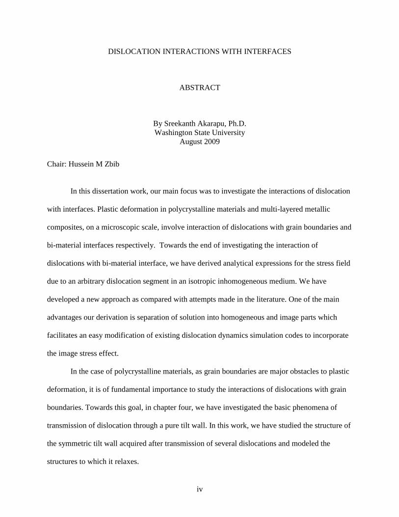
Figure 2.1 The plane cutting the unit sphere which is normal to the unit vector along relative

displacement vector. The anisotropic Greens tensor derivatives are integrated along the

peripheral circle of this plane. ............................................................................................... 21

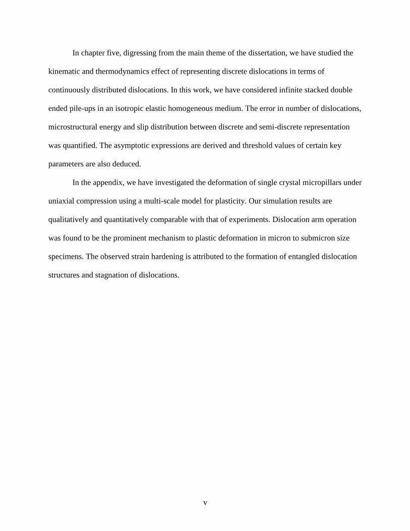
Figure 2.2 Infinite edge dislocation on the basal plane of Cu cubic crystal ................................. 22

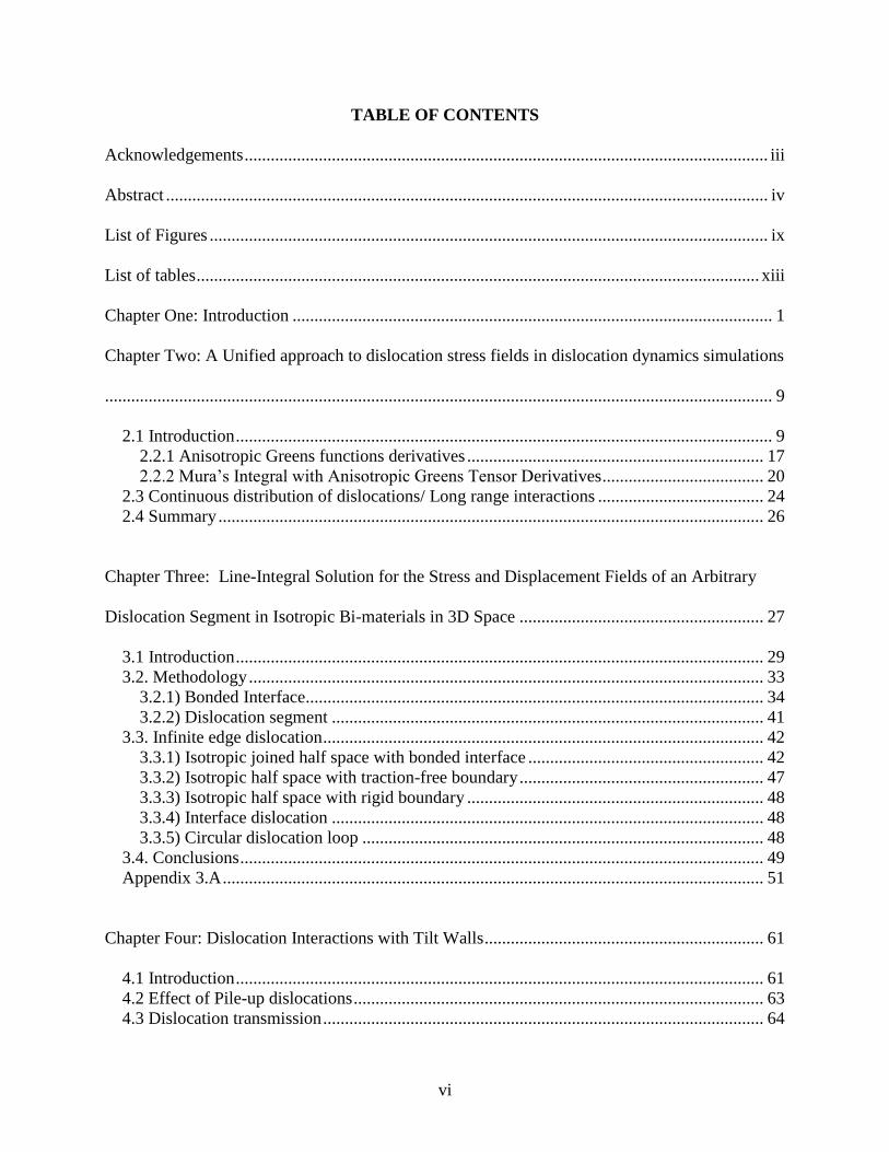
Figure 2.3 Comparison of shear stress component of an infinite edge dislocation oriented as

shown in figure 2.2 with ordinate in units of MPa and abscissa in units of 10b. The stress

computed from the numerical integration is validated with that of available analytical

solution. ................................................................................................................................. 23

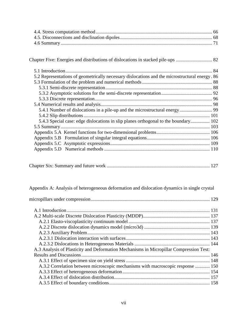
Figure 2.4 (a) An array of infinite edge dislocations with the surrounding rectangle denoting the

domain (axd) of homogenization (b) Comparison of shear stress due to the array of infinite

edge dislocations for different domains of homogenization with discrete solution. ............ 25

Figure 3.1 Joined Isotropic Half Spaces ....................................................................................... 53

Figure 3.2 Dislocation Segment .................................................................................................... 54

Figure 3.3 Comparison of image shear stress component of our solution „AZ Solution‟ with that

of Head solution due to an edge dislocation near a bi-material interface. ............................ 55

Figure 3.4 Comparison image shear stress component of our solution „AZ solution‟ with that of

Head solution due a edge dislocation near a traction-free surface ....................................... 56

Figure 3.5 Image shear stress component of an infinite edge dislocation near a rigid boundary . 57

Figure 3.6 Image shear stress component of an infinite edge dislocation in the interface ........... 58

Figure 3.7(a) Image shear stress component of a circular prismatic loop for different

discretizations ....................................................................................................................... 59

Figure 3.7(b) Vector plot of Peach-Koehler force on a circular glide loop .................................. 60

Figure 4.1(a) Infinite bi-crystal with pure tilt wall as the grain boundary (b) Evolution of

resolved shear stress in grain B (normalized by 3*10 2 1 ) as the dislocations pile

up in grain A against the grain boundary quantified as slip. ................................................ 73

Figure 4.2 Finite edge dislocation wall sheared by a perfect lattice dislocation to form a

disconnection in the boundary .............................................................................................. 74

Figure 4.3 Comparison of shear stress plot of finite edge dislocation wall computed analytically

with the numerical result using Mura‟s formula. The shear stress is normalized

with3*10

(1 )

. ................................................................................................................... 75

x

Figure 4.4(a) Finite edge dislocation wall (b) Finite wall with a multi-offset and a grain boundary

dislocation ............................................................................................................................. 76

Figure 4.5 Comparison of (a) Shear stress (normalized with 3*10

(1 )

) (b) strain energy

density (normalized with 2 15

1 *10

) plotted along a-a of finite edge dislocation

wall „Finite_Wall_a-a‟ (see Figure 3a) and an offset dislocation wall with a grain boundary

dislocation „Offset_mbd_4D_a-a‟ (see Figure 4.4b) ............................................................ 78

Figure 4.6(a) Dislocation structure formed after transmission of several dislocations through a

grain boundary (b) the configuration to which it relaxes (c) Configuration in which the GBD

is split into two at one-third positions from the center. ........................................................ 80

Figure 4.6(d) Comparison of strain energy density (normalized with 2 15

1 *10

)

plotted along a-a of finite walls with a large offset and a grain boundary dislocation

„Offset_mbd_4D_a-a‟ (see Figure 4.6(a)) and the relaxed configurations „Disconnection_a-

a‟ (see Figure 4.6(b)) and “Splitting GBD_a-a” (see Figure 4.6(c))..................................... 81

Figure 5.1 A thin film with single slip system and slip planes orthogonal to the boundary...... 113

Figure 5.2 A thin film with a single slip system embedded in an elastic space. Resolved shear

stress is prescribed. The slip planes are inclined at an angle with respect to 1x -axis.... 114

Figure 5.3 Function ,G c for 0, , ,6 4 3

(a) Edge dislocations. (b) Screw

dislocations. ........................................................................................................................ 115

Figure 5.4 Comparison of number of dislocations as computed from semi-discrete

representations (13) and the asymptotic expression (14). a) Edge dislocations: data includes

90, 36, 18, 12, 6, 3 b) Screw dislocations: data include

36, 6, 3 . ............................................................................................................. 116

Figure 5.5 Comparison of microstructural energy density (8) as computed from semi-discrete

representation with the asymptotic expression (20). Data include 36, 6, 3 . (a)

Edge dislocations. (b) Screw dislocations.......................................................................... 117

Figure 5.6 Comparison of number of dislocations as computed from discrete representation and

the asymptotic expression (14). (a) Edge dislocations. Data include

36, 18, 12, 6, 3 . (b) Screw dislocations. ................................................... 118

Figure 5.7 Comparison of energy densities computed from discrete representation (23) to

asymptotic expression (27), as function of the number of dislocations, 0N . ..................... 119

xi

Figure 5.8 Comparison of microstructural energy density (8) as computed from discrete

representation (23) with the asymptotic expression (27). (a) Edge dislocations. Data

include 36, 6, 3 . (b) Screw dislocations. ........................................................... 120

Figure 5.9 Slip distributions, as computed from discrete (symbols) and semi-discrete (lines)

representations for 6 = . Similar conclusions hold for 0 3 . (a) Edge

dislocations. (b) Screw dislocations. ................................................................................. 121

Figure 5.10a Slip distributions for different θ. (a) Edge dislocations – the number of

dislocations in the pile-up is minimal at 4 = corresponding to the distribution most

localized at the boundary. (b) Screw dislocations – the number of dislocations in the pile-up

decreases with , so that the most localized distribution is obtained for 0 = . ............... 122

Figure 5.11 Comparison of number of dislocations (13) and energy density (8) as computed from

semi-discrete representation with the asymptotic fit (28), as a function of . .................. 123

Figure 5.12 Comparison of number of dislocations and energy density (23) as computed from

discrete representation with the asymptotic fit (29), as a function of . The scatter of

data indicates different values of . ................................................................................... 124

Figure 5.13 Comparison of slip distributions, as computed from discrete (symbols), and semi-

discrete (lines) representations. ........................................................................................... 125

Figure A.1. Multiscale Dislocation Dynamics Plasticity Model: Coupling of dislocation

dynamics with continuum elasto-visoplasticty ................................................................... 165

Figure A.2. a, b and c are random distributions of Frank-Read sources and dislocation arms as

initial dislocation structure of the order of 1013

(1/m2) for specimen sizes of 0.5, 1.0 and 2.0

micron respectively (see Table 2 for color coding); d, e and f are the corresponding

dislocation structures after 1.0%, 0.8% and 0.5% strain, respectively. ............................. 166

Figure A.3. Stress-strain behavior of Cu specimens with thickness ranging from 0.2 microns to

2.5 microns .......................................................................................................................... 167

Figure A.4(a). A log-log plot of normalized yield stress 2y

as a function of specimen size

at various %strain offsets (closed symbols); the open symbols represent the critical stress

with and without the effect of image stresses to operate a single arm; the lines represent the

data from equation A.11 for various n and .................................................................... 168

Figure A.4(b) log-log plot of yield stress normalized with shear modulus 2y

of respective

material ( Au = 27GPa, Ni = 76GPa and Cu = 48.3 GPa) vs. specimen size in microns;

Comparison of the experimental data of Au, Cu and Ni micropillar compression is made

with simulation result at 0.02% and 0.4% strain offset and the data from equation A.11 .. 169

xii

Figure A.5. a) Schematic depicting the operation of dislocation arm. b) Side view of the

dislocation arm. c) Schematic of dislocation arm structure acting as a spiral source. d) Snap

shot of spiral source (see Table 2 for coloring) .................................................................. 170

Figure A.6. Evolution of dislocation density in specimens with thickness ranging from 0.2

microns to 2.5 microns ........................................................................................................ 171

Figure A.7. a) Snapshot of an immobile dislocation structure during elastic loading of 0.5

micron thick specimen (see Table 2 for color coding) b) Schematic explaining the process

of formation of an entangled dislocation structure (see Table 2 for coloring) ................... 172

Figure A.8a-b. Correlation among stress drop, dislocation bursts, cross-slip and dislocation

interactions, for the 0.5 microns thick specimen. The vertical axis in Figure A.8(b) denotes

the number of jogs, junctions and cross-slip events occurred during the process of

deformation. Note: a cross-slip node is where a dislocation line changes slip-plane as a

result of a cross-slip event, e.g. node B in Figure A.5c. Two cross-slip nodes form when a

screw dislocation segment cross-slip from its primary glide plane to a secondary plane to

overcome an obstacle or a pinning site, such as junction or a stress concentration site. .... 173

Figure A.9. a) Contour of percentage effective plastic strain of the deformed 0.5 microns thick

specimen. b) The stress contour of the component along the z-axis/loading axis depicting

the stress concentration at the ledges on the surface. c) Schematic showing the effect of

stress concentration at the surface. ...................................................................................... 175

Figure A.10. Effect of image stress; comparison of the behavior of a 0.5 micron thick specimen

using DD and MDDP, a) stress-strain response, b) evolution of dislocation density, c)

evolution of number of dislocation segments that are parts of junctions (junction segments),

and “cross-slip nodes”, a cross-slip node is where a dislocation line changes slip-plane as a

result of a cross-slip event, e.g. node B in Figure 5c. The initial dislocation density in these

simulations is 1014

/m2 ........................................................................................................ 177

Figure A.11. Sensitivity of stress-strain response to the distribution of dislocation with same

density of (1013

1/m2) in 0.5 micron specimen ................................................................... 178

Figure A.12. Effect of boundary conditions, no friction versus sticking friction. The simulations

were performed for the same specimen with same dislocation distribution and density of

1013

1/m2 in 0.5 micron thick specimen. [Note: The displacement field in the deformed

configurations is magnified by factor of 10 for better visualization] ................................. 179

xiii

LIST OF TABLES

Table 5.1 Conditions for validity of asymptotic expressions (5.30). ......................................... 126

Table A.1 Material and control parameters of the simulation .................................................... 164

Table A.2 Coloring legend of dislocations ................................................................................. 164

xiv

Dedication

I dedicate this dissertation to my

GGGrrraaannndddmmmooottthhheeerrr::: LLLaaattteee SSSrrreeeeeerrraaammmooojjjuuu UUUdddaaayyyaaa LLLaaakkkssshhhmmmiii

GGGrrraaannndddfffaaattthhheeerrr::: SSSrrreeeeeerrraaammmooojjjuuu SSSrrreeeeeesssaaaiiilllaaammm

FFFaaattthhheeerrr::: AAAkkkaaarrraaapppuuu JJJaaannnaaarrrdddhhhaaannn RRRaaaooo

MMMooottthhheeerrr::: AAAkkkaaarrraaapppuuu RRReeennnuuukkkaaa DDDeeevvviii aaannnddd

BBBrrrooottthhheeerrr::: AAAkkkaaarrraaapppuuu RRRaaavvviiinnndddrrraaa KKKuuummmaaarrr

1

CHAPTER ONE: INTRODUCTION

Modeling of plastic deformation of metals under extreme loading conditions depends

mainly on our knowledge of microscopic mechanisms and their influence on the

macroscopic response. In plastic deformation, dynamics of dislocations which pattern

into various dislocation structures are the key microscopic phenomena which influence

the macroscopic behavior. Towards the goal of understanding plastic deformation from

the more physical perspective, various researchers have established discrete models to

investigate the origin of dislocation structures by perceiving the problem as a dynamical

evolution of dislocations in deforming crystals. Some of the most original models were

two-dimensional based on periodic cells each with infinite edge dislocations. Although

these 2D models have shed light on glide mechanisms of dislocations, they lacked the

incorporation of important mechanisms such as cross-slip, jogs, junctions and line tension

associated with curvature of dislocations. These issues of more idealistic 2D models were

addressed in a pioneering work by (Kubin et al. 1992) on the development of three

dimensional dislocation models. In their model, the dislocation curves are discretized into

pure edge and pure screw dislocation segments. (Zbib et al. 1996a) have established a

new approach for three dimensional dislocation dynamics (3D-DD) by discretizing

arbitrarily curved dislocations into piecewise continuous arrays of mixed dislocation

segments. The dynamical evolution of these dislocation segments on their respective

crystallographic planes is determined by solving the first order differential equation

consisting of an inertia term, a drag term and a driving force vector as given by

2

*

,

DD i

s i i

vm v F

M T p (1.1)

In the above equation, the subscript s stands for the segment, m* is the effective

dislocation segment mass density given by (Hirth et al. 1998a), M is the dislocation

mobility which could depend both on the temperature T and the pressure p. The driving

force Fi per unit length arises from a variety of sources. Since the strain field of the

dislocation varies as the inverse of the distance from the dislocation core, dislocations

interact among themselves over long distances, yielding a dislocation-dislocation

interaction force FD. A moving dislocation has to overcome local constraints such as the

Peierls stresses (i.e. lattice friction), FPeierls. The dislocation may encounter local obstacles

such as stacking fault tetrahedra, defect clusters and vacancies that interact with the

dislocation at short ranges, giving rise to a dislocation-obstacle interaction force FObstacle.

Furthermore, the internal strain field of randomly distributed local obstacles gives rise to

stochastic perturbations to the encountered dislocations, as compared with deterministic

forces such as the applied load. This stochastic stress field, or thermal force FThermal

arising from thermal fluctuations, also contributes to the spatial dislocation patterning in

the later deformation stages. Dislocations also interact with free surfaces, cracks, and

interfaces, giving rise to what is termed as image stresses or forces FImage. In addition, a

dislocation segment feels the effect of externally applied loads, FExternal, osmotic force

FOsmotic resulting from non-conservative motion of dislocation (climb) and its own self-

force FSelf. Adding all of these effects together yields the following expressions for the

driving force in (1.1).

ThermalOsmoticImageObstacleExternalSelfDPeirelsi FFFFFFFFF (2.1)

3

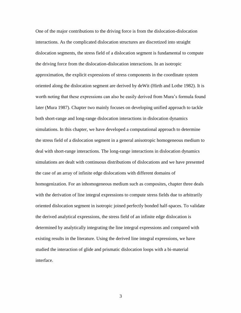
One of the major contributions to the driving force is from the dislocation-dislocation

interactions. As the complicated dislocation structures are discretized into straight

dislocation segments, the stress field of a dislocation segment is fundamental to compute

the driving force from the dislocation-dislocation interactions. In an isotropic

approximation, the explicit expressions of stress components in the coordinate system

oriented along the dislocation segment are derived by deWit (Hirth and Lothe 1982). It is

worth noting that these expressions can also be easily derived from Mura‟s formula found

later (Mura 1987). Chapter two mainly focuses on developing unified approach to tackle

both short-range and long-range dislocation interactions in dislocation dynamics

simulations. In this chapter, we have developed a computational approach to determine

the stress field of a dislocation segment in a general anisotropic homogeneous medium to

deal with short-range interactions. The long-range interactions in dislocation dynamics

simulations are dealt with continuous distributions of dislocations and we have presented

the case of an array of infinite edge dislocations with different domains of

homogenization. For an inhomogeneous medium such as composites, chapter three deals

with the derivation of line integral expressions to compute stress fields due to arbitrarily

oriented dislocation segment in isotropic joined perfectly bonded half-spaces. To validate

the derived analytical expressions, the stress field of an infinite edge dislocation is

determined by analytically integrating the line integral expressions and compared with

existing results in the literature. Using the derived line integral expressions, we have

studied the interaction of glide and prismatic dislocation loops with a bi-material

interface.

4

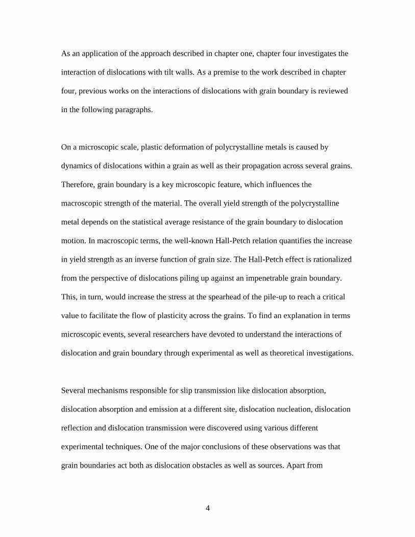
As an application of the approach described in chapter one, chapter four investigates the

interaction of dislocations with tilt walls. As a premise to the work described in chapter

four, previous works on the interactions of dislocations with grain boundary is reviewed

in the following paragraphs.

On a microscopic scale, plastic deformation of polycrystalline metals is caused by

dynamics of dislocations within a grain as well as their propagation across several grains.

Therefore, grain boundary is a key microscopic feature, which influences the

macroscopic strength of the material. The overall yield strength of the polycrystalline

metal depends on the statistical average resistance of the grain boundary to dislocation

motion. In macroscopic terms, the well-known Hall-Petch relation quantifies the increase

in yield strength as an inverse function of grain size. The Hall-Petch effect is rationalized

from the perspective of dislocations piling up against an impenetrable grain boundary.

This, in turn, would increase the stress at the spearhead of the pile-up to reach a critical

value to facilitate the flow of plasticity across the grains. To find an explanation in terms

microscopic events, several researchers have devoted to understand the interactions of

dislocation and grain boundary through experimental as well as theoretical investigations.

Several mechanisms responsible for slip transmission like dislocation absorption,

dislocation absorption and emission at a different site, dislocation nucleation, dislocation

reflection and dislocation transmission were discovered using various different

experimental techniques. One of the major conclusions of these observations was that

grain boundaries act both as dislocation obstacles as well as sources. Apart from

5

investigating the dislocation interactions with grain boundaries using dynamic in-situ

TEM, (Shen et al. 1998) proposed criteria to predict the conditions for slip propagation

across the grain boundary. According to this work, the slip plane of the emitted

dislocation is predicted from the minimum angle between lines traced by the incoming

and outgoing slip planes on the boundary plane and the slip direction is predicted using

the criteria of maximum resolved shear stress on the emitted slip plane.

Using in situ TEM deformation study, another significant contribution was made by (Lee

et al. 1990) in studying the interactions of glissile dislocations with grain boundary. In

this work, they have proposed modified criteria to predict the slip system for the slip

transmission phenomena. According to (Lee et al. 1990), the angle between the traces of

the slip planes and grain boundary should be a minimum, the resolved shear stress on the

slip planes in the adjoining grain should be a maximum and the magnitude of the residual

dislocation left in the grain boundary should be a minimum. Unlike the criteria of (Shen

et al. 1998), the slip direction is determined considering not only by the maximum

resolved shear stress but also the minimum residual left at the boundary.

Computational modeling of deformation of polycrystalline solids is a highly complicated

task as it is controlled by simultaneous processes occurring at various length and time

scales. Thus, it is imperative to develop a multi-scale approach by passing information

from one scale to another. In the case of single crystal plasticity, the unit dislocation

mechanisms such as dislocation short-range reactions and dislocation mobility were

studied using atomistic simulations and passed to higher scale dislocation dynamics

6

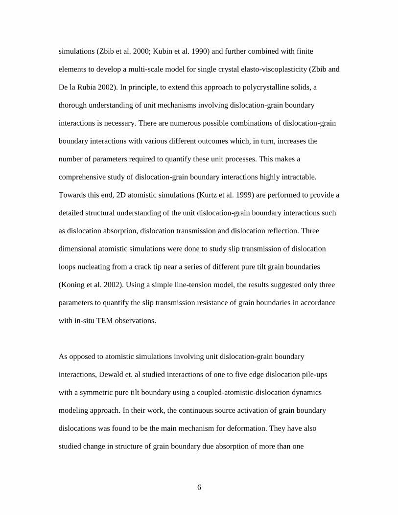
simulations (Zbib et al. 2000; Kubin et al. 1990) and further combined with finite

elements to develop a multi-scale model for single crystal elasto-viscoplasticity (Zbib and

De la Rubia 2002). In principle, to extend this approach to polycrystalline solids, a

thorough understanding of unit mechanisms involving dislocation-grain boundary

interactions is necessary. There are numerous possible combinations of dislocation-grain

boundary interactions with various different outcomes which, in turn, increases the

number of parameters required to quantify these unit processes. This makes a

comprehensive study of dislocation-grain boundary interactions highly intractable.

Towards this end, 2D atomistic simulations (Kurtz et al. 1999) are performed to provide a

detailed structural understanding of the unit dislocation-grain boundary interactions such

as dislocation absorption, dislocation transmission and dislocation reflection. Three

dimensional atomistic simulations were done to study slip transmission of dislocation

loops nucleating from a crack tip near a series of different pure tilt grain boundaries

(Koning et al. 2002). Using a simple line-tension model, the results suggested only three

parameters to quantify the slip transmission resistance of grain boundaries in accordance

with in-situ TEM observations.

As opposed to atomistic simulations involving unit dislocation-grain boundary

interactions, Dewald et. al studied interactions of one to five edge dislocation pile-ups

with a symmetric pure tilt boundary using a coupled-atomistic-dislocation dynamics

modeling approach. In their work, the continuous source activation of grain boundary

dislocations was found to be the main mechanism for deformation. They have also

studied change in structure of grain boundary due absorption of more than one

7

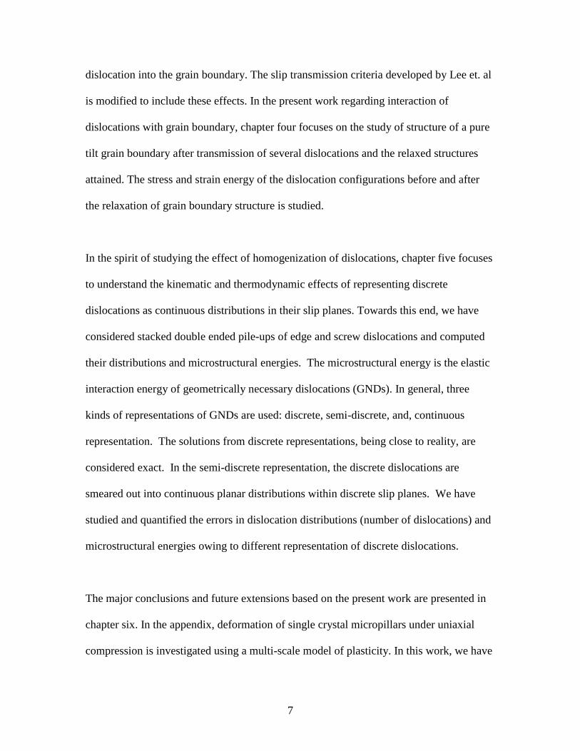
dislocation into the grain boundary. The slip transmission criteria developed by Lee et. al

is modified to include these effects. In the present work regarding interaction of

dislocations with grain boundary, chapter four focuses on the study of structure of a pure

tilt grain boundary after transmission of several dislocations and the relaxed structures

attained. The stress and strain energy of the dislocation configurations before and after

the relaxation of grain boundary structure is studied.

In the spirit of studying the effect of homogenization of dislocations, chapter five focuses

to understand the kinematic and thermodynamic effects of representing discrete

dislocations as continuous distributions in their slip planes. Towards this end, we have

considered stacked double ended pile-ups of edge and screw dislocations and computed

their distributions and microstructural energies. The microstructural energy is the elastic

interaction energy of geometrically necessary dislocations (GNDs). In general, three

kinds of representations of GNDs are used: discrete, semi-discrete, and, continuous

representation. The solutions from discrete representations, being close to reality, are

considered exact. In the semi-discrete representation, the discrete dislocations are

smeared out into continuous planar distributions within discrete slip planes. We have

studied and quantified the errors in dislocation distributions (number of dislocations) and

microstructural energies owing to different representation of discrete dislocations.

The major conclusions and future extensions based on the present work are presented in

chapter six. In the appendix, deformation of single crystal micropillars under uniaxial

compression is investigated using a multi-scale model of plasticity. In this work, we have

8

considered micropillars with sizes ranging from 0.2 to 2.5 microns and predicted size

effects. The simulation results are qualitatively as well as quantitatively compared with

the experiments.

9

CHAPTER TWO: A UNIFIED APPROACH TO DISLOCATION STRESS

FIELDS IN DISLOCATION DYNAMICS SIMULATIONS

2.1 Introduction

In recent times, three dimensional discrete dislocation dynamics simulations have gained

a lot of impetus in understanding many key dislocation mechanisms and their influence

on the macroscopic plastic deformation in both single crystals as well as inhomogeneous

medium like bi-materials and nano-metallic multi-layered composites. In dislocation

dynamics simulations, the dynamics of dislocations on their respective crystallographic

planes are evolved under the influence of the external agents and the internal stress due to

other dislocations, defects and obstacles. Among all the driving forces for the dynamics

of dislocations, the contribution of dislocation-dislocation interactions is quite significant.

These simulations deal with high density of dislocations and complicated dislocation

configurations. To compute the dislocation-dislocation interactions, the stress field of a

general curved dislocation in a general anisotropic medium is crucial. A brief review of

different methodologies to efficiently compute the stress field of general curved

dislocations is presented.

A general theory was developed by (Indenbom and Orlov 1967; Indenbom and Orlov

1968) and for a simpler planar case by (Brown 1967) for the computation of deformation

and stress field of curved dislocations. From physical arguments, as a dislocation segment

by itself has no physical meaning, (Indenbom and Orlov 1967) has introduced elementary

10

configurations such as elementary loop, semi-dipole and hairpin. The stress field of semi-

dipole is synthesized from the solution of the elementary loop and, in the same way; the

solution of hairpin dislocation configuration is synthesized from the solution of semi-

dipole configuration. Instead of dealing with isolated dislocation segment which is

physically non-existent, (Indenbom and Orlov 1967) dealt with hairpin configuration as

the physically complete basic ingredient. As the stress field of an infinite straight

dislocation at a field point can be constructed from a collection of infinitely many hairpin

configurations with the field point as the common apex, the stress field of the hairpin

configuration is expressed in terms of infinite straight dislocation stress factors and its

derivatives. This idea and methodology is essentially similar to that originally presented

by (Brown 1967). (Brown 1967) has derived a formula to compute the stress field at a

point in the plane of a planar loop in terms of infinite straight dislocation stress factors

and its derivatives similar to (Indenbom and Orlov 1967). A remarkable feature of

Brown‟s formula for the planar case is that it can be integrated over a straight dislocation

segment. (Indenbom and Orlov 1967; Indenbom and Orlov 1968) independently extended

this theory to a more general non-coplanar case. The Indenbom-Orlov-Brown theory is

most general and valid even for general anisotropic medium. Although, theoretically,

Brown-Indenbom-Orlov formula is very convenient in that they have nice features such

as semi-rational dislocation elements and transparent connections to energy relations,

their actual numerical implementation is quite difficult.

As the Indenbom-Orlov-Brown theory expresses its solution in terms of infinite straight

dislocation stress factors and its derivatives, for anisotropic cases, an elegant approach to

11

deal with straight dislocations in anisotropic media is the key factor. (Stroh 1962)

extended the theory developed by (Eshelby et al. 1953) and developed an elegant and

powerful six dimensional eigenvector theory often referred as sextic theory. Later,

(Barnett and Lothe 1973) developed an integral theory by transforming Stroh‟s six

dimensional eigenvector theory. The sextic theory relies on numerical solution of six

dimensional eigenvalue problem where as the integral theory relies on numerical

integration of certain definite integrals. Computationally, the numerical evaluation of

eigenvalue problem is difficult compared to numerical quadrature. Later (Rhee et al.

2001) developed look up tables by numerically integrating the angular stress factors and

its derivatives derived by (Asaro and Barnett 1973). These look up tables were used to

deal with anisotropic stress fields in dislocation dynamics simulation code.

Alternatively, (Willis 1970) and (Steeds 1973) developed theories in the spirit of

mathematical simplicity and explicitness as compared with work of Indenbom-Orlov-

Brown theories. Within a much simpler framework, (Mura 1987) derived the line

integrals for the stress fields due to a dislocation segment in a general anisotropic

medium using Fourier analysis with eigenstrain method. These integrals are also naturally

extended to continuous distribution of dislocations. In the spirit of easy implementation

in computer simulation, as suggested by Lothe, the simplest procedure to find the stress

field of an arbitrarily oriented dislocation segment in a general anisotropic medium is the

combination of Mura‟s integral formula with anisotropic Green‟s function derivatives.

12

To tackle the short-range as well as long-range interactions of dislocations, in this

chapter, we have presented a unified approach following Mura‟s methodology for both

homogeneous general anisotropic medium and isotropic inhomogeneous medium. In

section 2.2, we present the approach employed to find the stress field of dislocation

segment in a general anisotropic medium by numerically integrating the Green‟s function

derivatives and combining them with Mura‟s line integral. The short-range interactions of

dislocation configurations can be addressed by this approach. In section 2.3, we suggest

the use of continuous distribution of dislocations to address the long-range interactions of

dislocations. Here, we consider an array of straight infinite edge dislocations to illustrate

the effect of homogenization of the stress field distribution. In section 2.4, we summarize

the approach for homogeneous case along with presenting the line integrals derived for

inhomogeneous case in the chapter three.

2.2 Discrete dislocations/Short range interactions

In this section, according to (Mura 1987), we present the formal derivation of the line

integral for the stress field due to a dislocation segment in a general anisotropic medium.

In the presence of a dislocation loop in an infinite homogeneous medium, the

displacement gradient iju is assumed to consist of elastic distortion ji and plastic

distortion p

ji .

p

ij ji jiu (2.1)

13

The elastic distortion ji is caused by the presence of eigenstrain/plastic distortion due to

the dislocation loop. According to linear elasticity, using Hooke‟s law, the stress field

caused due to the presence of dislocation loop is due to the elastic distortion ji given by

ij ijkl lkC (2.2)

where ij

and ijkl

C are the components of symmetric second order stress tensor and fourth

order stiffness tensor.

According to the principle of conservation of linear momentum, the stress must satisfy

the following equilibrium equations

,0

jij (2.3)

Using (2.2) and (2.1), the equilibrium equations in terms of displacement gradient is give

by

, ,0

lj j

p

ijkl k ijkl lkC u C (2.4)

The second term in the above equation is perceived as a body force due to the presence of

eigenstrain strain caused by dislocation loop. Using the method of Greens function, the

displacement solution due to the body force , j

p

ijkl lkC is given by

( )( ) ( , )

p

nm

i ip pqmn

q

xu x G x x C dx

x

(2.5)

The second rank tensor ,ij

G x x is defined as the mapping between the displacement

response in the i direction at x due to the thj component of the point force acting at x in

an infinite medium. This mapping, Greens tensor, satisfies the following equilibrium

equations given as

14

( , )

0pi

mnpq mi

q n

G x xC x x

x x

(2.6)

where is a Dirac‟s delta function.

Using Guass theorem, (2.5) can be expressed as

( , )( ) ( )

ip p

i pqmn nm

q

G x xu x C x dx

x

(2.7)

By taking the first derivative of displacement, using (2.7), the displacement gradient can

be expressed as

,

( , )( ) ( )

j

ip p

i pqmn nm

q j

G x xu x C x dx

x x

(2.8)

Using (2.1), (2.8) can rewritten as an expression for elastic distortion

( , )( ) ( ) ( )

ip p p

ji pqmn nm ji

q j

G x xx C x dx x

x x

(2.9)

Using (2.6), the plastic distortion p

jix can be expressed as

( , )

( ) ( ) ( )pip p p

ji jm mi mnpq jm

q n

G x xx x x x dx C x dx

x x

(2.10)

Substituting (2.10) into (2.9), we have

( , ) ( , )( ) ( ) ( )

ip pip p

ji pqmn nm mnpq jm

q j q n

G x x G x xx C x dx C x dx

x x x x

(2.11)

The above equation is the most general solution for the elastic distortion for any medium

provided the knowledge of Greens tensor function for a point source in the medium. For a

general anisotropic homogeneous medium, few key properties of Greens tensor function

15

enable the transformation of (2.11) into a line integral over the dislocation segment. The

Greens function for a general homogeneous medium is a function of relative

displacement vector and a symmetric second order tensor. Mathematically, the equations,

which hold true for Green‟s tensor and its derivatives, for homogenous medium, are

, ( ) ( )ip ip pi

G x x G x x G x x (2.12)

( ) ( )ip ip

j j

G x x G x x

x x

(2.13)

( ) ( )ip ip

q n q n

G x x G x x

x x x x

(2.14)

Using the properties (2.12)-(2.14), (2.11) can be written as

( ) ( )( ) ( ) ( )

ip ipp p

ji pqmn nm mnpq jm

q j q n


x x x x

(2.15)

Using Gauss theorem and properties (2.12)-(2.14), (2.15) can be expanded as

,

, ,

,

( ) ( ) ( )

( ) ( )j n

ip ipp p

ji mnpq jm pqmn nm

q qn j

ip p p

pqmn nm jm

q


x x

G x xC x x dx

x

(2.16)

The first two terms in (2.16) vanish at infinity and reduces to

, ,( ) ( ) ( )

j n

ip p p

ji pqmn nm jm

q

G x xx C x x dx

x

(2.17)

According to (Kroner 1958), the dislocation density tensor defined as the curl of plastic

distortion can be easily shown to satisfy

, ,( )

n j

p p

jnh hm jm nmx (2.18)

Using (2.18) and (2.13), (2.17) can be written as

16

( )

( )ip

ji jnh pqmn hm

q

G x xx C x dx

x

(2.19)

The dislocation density tensor hm

quantifies the mth

component of total Burgers vector

of all the dislocation intersecting the plane whose normal is in the h direction.

Mathematically, the dislocation density tensor hm

is expressed as

hm h mdx b dl (2.20)

Using (2.20), the volume integral for elastic distortion can be transformed into a line

integral over the dislocation segment given as

( )

ip

ji jnh pqmn m hl

q

G x xx C b dl

x

(2.21)

Thus, the stress due to an arbitrary dislocation segment in a general homogenous

anisotropic medium can be expressed as a line integral over the dislocation line as

( )

kp

ij ijkl lnh pqmn m hl

q

G x xx C C b dl

x

(2.22)

For explicit evaluation of stress by integrating (2.22), the knowledge of Greens function

derivatives is essential. For an isotropic approximation, the convenient explicit

expressions are given by (Mura 1987)

, 1 1 2 2 3 3

1 3

1

5

( , , )

( ) ( ) ( )1(1 2 )

8 (1 )

( )( )( )3

qpqmn ip

ni m m im n n mn i i

m m n n i i

C G x x x x x x

x x x x x x

R

x x x x x x

R

(2.23)

where

2 2 2

1 1 2 2 3 3( ) ( ) ( )R x x x x x x

17

For a general anisotropic homogeneous medium, there are no explicit expressions for

Greens function derivatives. Several attempts have been made to find approximate

expressions. In the following sub-section, we present a brief review of the work of

(Barnett 1972) on evaluation of anisotropic Greens function derivatives using Fourier

transform method.

2.2.1 Anisotropic Greens functions derivatives

Using Fourier transform method, (Barnett 1972) has extended the well-documented

method of finding Greens functions by solving (2.6) to its first and second derivatives. In

this section, for the sake of completeness, we briefly present the method derived in

(Barnett 1972). Rewriting (2.6),

( )

0km

ijkl mi

j l

G x xC x x

x x

(2.24)

Using Fourier integral transform, the Dirac delta function can be represented as

. 3

3

1

2

i x xx x e d

(2.25)

Similarly, the Greens tensor can be represented using Fourier integral representation as

. 3

3

1

2

i x x

km kmG x x g e d

(2.26)

where g

,

and are Fourier amplitude of Greens tensor, wave vector and its

magnitude respectively. Substituting (2.26) and (2.25) in (2.24), Greens tensor Fourier

amplitude satisfies

0j ijkl l km miC g

(2.27)

Denoting ik j ijkl lK C

and 1*

ik ikK K

, the Fourier amplitude can be written as

18

*

2

ij

ij

Kg

(2.28)

where

is the unit vector along the wave vector

.

Substituting (2.28) in (2.26), Greens tensor can be written as

*

. 3

3 2

1

2

i x xkm

km

KG x x e d

(2.29)

Considering only the real part of (2.29),

*

3

3 2

1cos .

2

km

km

KG x x x x d

(2.30)

and the first derivatives can be expressed as

*

3

3

1sin .

2

j kmkm

j

KG x xx x d

x

(2.31)

Let

and R be the unit vector along x x and its magnitude respectively and (2.31)

can be re-written as

*

3

3

1sin .

2

j kmkm

j

KG x xR d

x

(2.32)

Changing variables to R

, 3 3 3d R d ,

, (2.32) becomes

*

3

3 2

1sin .

2

j kmkm

j

KG x xd

x R

(2.33)

The triple integral in (2.33) can be transformed into a line integral about a unit circle in

the plane . 0

using spherical polar coordinate system aligned along

. The volume

element can be expressed as 3 2 sind d d d with . cos

where being

19

the polar angle in the plane . 0

.Using spherical polar coordinates, (2.33) can be

written as

*

3 2

1sin cos sin

2

km

j km

j

G x xK d d d

x R

(2.34)

Considering integration of (2.34) over and noting that

0 0

sin cos cos cos coscos sin

d d

(2.35)

The result of the integration over is given as

*

3 2

2

*

2 2

0 0

1sin cos sin

2

1cos

8

j km

j km

K d d dR

d d KR

(2.36)

2 2

* *

2 2 2 22

0 0 0

1 1cos

8 8j km j kmd d K K d

R R

(2.37)

Considering the integrand in (2.37) and using product rule,

*

* *

22 2

j kmj km km j

KK K

(2.38)

Noting that

2

j

j

(2.39)

and differentiating ik j ijkl lK C

with respect to ,

ij l kijkl k l

KC

(2.40)

20

** *km rskr sm

K KK K

(2.41)

Using (2.39), (2.40) and (2.41) in (2.38),

* * * *

2j km j km j kr sm ijkl k l k lK K K K C

(2.42)

Using (2.42), the first derivatives of Greens tensor can expressed as

2

* * *

2 2

0

1

8

kmj km j kr sm ijkl k l k l

j

GK K K C d

x R

(2.43)

2.2.2 Mura’s Integral with Anisotropic Greens Tensor Derivatives

In our work, as suggested by Lothe, we have combined the Mura‟s integral (2.22) with

anisotropic Greens function derivatives (2.43) to provide a simplest possible approach to

tackle the short range interactions of dislocations in a general anisotropic medium. The

Greens tensor function derivatives given by the line integral in (2.43) is integrated over a

periphery of a plane cutting a unit sphere. The normal to this plane is the unit vector

along the relative displacement vector. As the integration is done on the boundary of

plane . 0

, a general wave vector

which lies only on this plane is considered (see

figure 2.1).

21

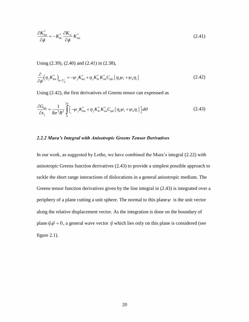
Figure 2.1 The plane cutting the unit sphere which is normal to the unit vector along

relative displacement vector. The anisotropic Greens tensor derivatives are integrated

along the peripheral circle of this plane.

For the numerical integration of Mura‟s line integral, for each quadrature point in the

linear domain of the dislocation segment, a right-handed orthogonal triad

is

formed for the integration of Greens tensor function derivatives. The components of a

general unit vector

with respect to

can be expressed as

cos sin (2.44)

Using spherical polar coordinate system, the mapping between the trial

and the

global Cartesian coordinate system can be determined by expressing the components

of

,

and

as

1 2 3

1 2 3

1 2 3

sin cos , sin sin , cos

sin , cos , 0

cos cos , cos sin , sin

(2.45)

where and are the angular spherical polar coordinates.

. 0

22

For the numerical integration of Greens function derivatives, using the mapping defined

in (2.45), the integrand which is a function of

is expressed with respect to global

Cartesian coordinate system.

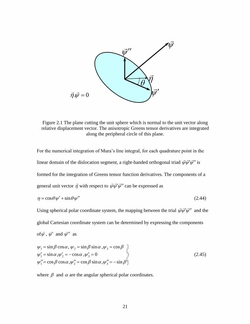
To validate the above described approach to compute the stress fields of discrete

dislocations to tackle the short range interactions, we considered an infinite edge

dislocation on the basal plane of Cu cubic crystal (see figure 2.2). The material Cu is

chosen due to its considerably high anisotropy factor.

Figure 2.2 Infinite edge dislocation on the basal plane of Cu cubic crystal

Derivation of exact analytical expressions requires the analytical solutions for the roots of

the six dimensional eigenvalue problems or analytical integration of integrals in the

integral formalism. Although it is a very difficult task for a general case, for the case of

100

010

001

23

high symmetry crystals and symmetrical orientation of the dislocation line, analytical

expressions have been documented in (Indenbom and Lothe 1992). The analytical

expressions for the case considered for the validation of the approach are documented in

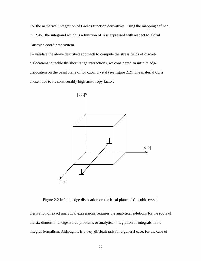
(Indenbom and Lothe 1992). As it can be seen in figure 2.3, the shear stress computed by

numerically integrating the Mura‟s integral in conjunction with numerically integrated

Greens tensor derivatives validates well with the available analytical solutions. It is worth

noting that the short range anisotropic stress field is significantly different from the

isotropic approximation. But, after about 80 units of Burgers vector magnitude, the

anisotropic stress field converges to isotropic approximation.

Figure 2.3 Comparison of shear stress component of an infinite edge dislocation oriented

as shown in figure 2.2 with ordinate in units of MPa and abscissa in units of 10b. The

stress computed from the numerical integration is validated with that of available

analytical solution.

-250

-200

-150

-100

-50

0

50

100

150

200

250

-25 -20 -15 -10 -5 0 5 10 15 20 25

Distance (in units of 10b)

Sh

ea

r s

tre

ss

(MP

a)

Isotropic

Anisotropic

Analytical_Anisotropic

12

24

2.3 Continuous distribution of dislocations/ Long range interactions

Using the same approach, we propose to deal with long range interactions in dislocation

dynamics by representing the ensemble of dislocations in the form of dislocation density

tensor. As described above, the stress field of continuous distribution of dislocations can

be computed by numerically integrating the Mura‟s formula given by

, hmij pqmnijkl lnh kp q

V

x C C G x x dV

(2.46)

where V is the volume over which the dislocations are homogenized and the dislocation

density tensor defined in (2.20) is rewritten as

hm m hdV b dl (2.47)

25

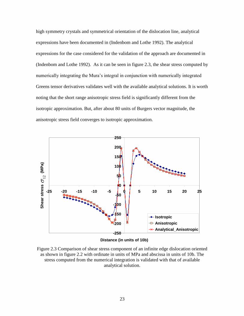
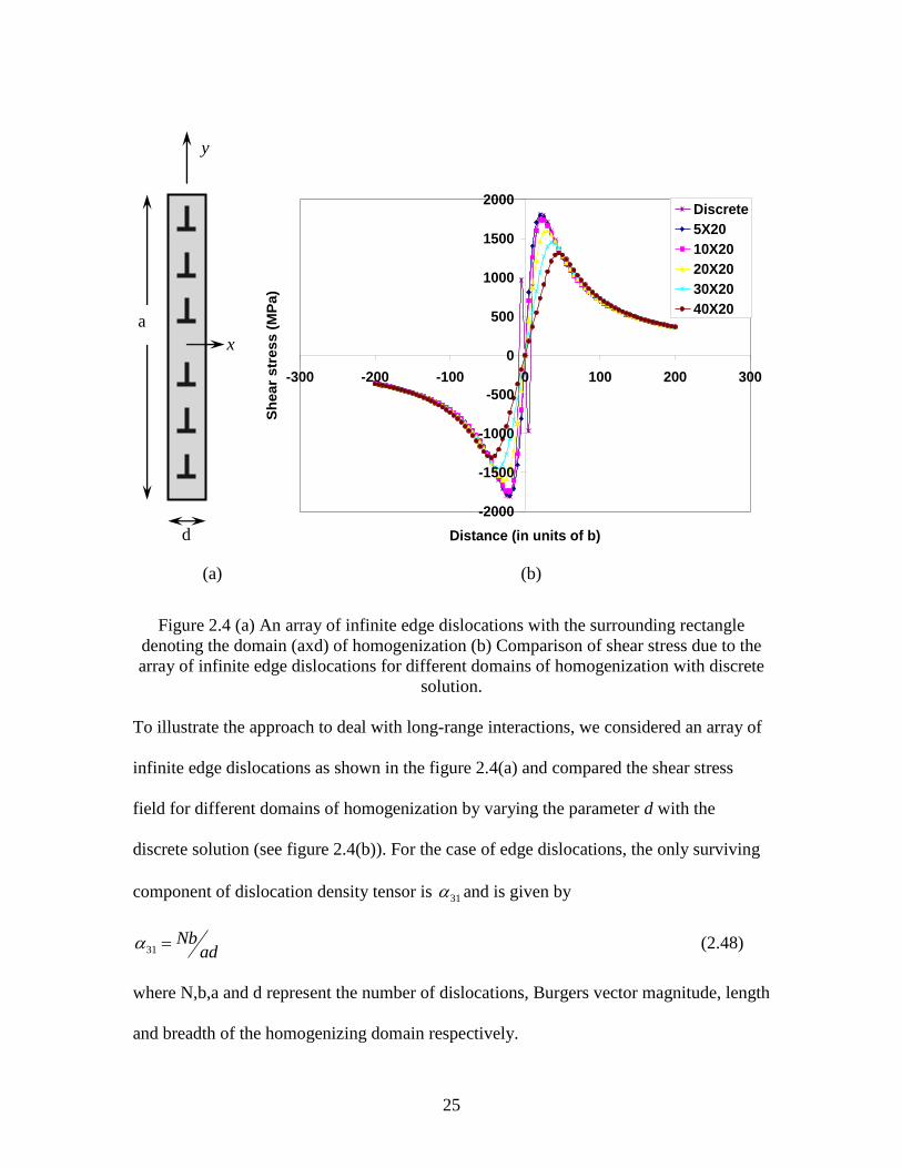
Figure 2.4 (a) An array of infinite edge dislocations with the surrounding rectangle

denoting the domain (axd) of homogenization (b) Comparison of shear stress due to the

array of infinite edge dislocations for different domains of homogenization with discrete

solution.

To illustrate the approach to deal with long-range interactions, we considered an array of

infinite edge dislocations as shown in the figure 2.4(a) and compared the shear stress

field for different domains of homogenization by varying the parameter d with the

discrete solution (see figure 2.4(b)). For the case of edge dislocations, the only surviving

component of dislocation density tensor is 31 and is given by

31Nb

ad (2.48)

where N,b,a and d represent the number of dislocations, Burgers vector magnitude, length

and breadth of the homogenizing domain respectively.

-2000

-1500

-1000

-500

0

500

1000

1500

2000

-300 -200 -100 0 100 200 300

Distance (in units of b)

Sh

ear

str

ess (

MP

a)

Discrete

5X20

10X20

20X20

30X20

40X20

x

y

a

d

(a) (b)

26

As it can be seen from the figure 2.4(b), the stress field due to the homogenized

dislocations approaches the discrete solution with the decrease of the domain of

homogenization. The stress field due to discrete array and distributed dislocation density

converges to the same value after about 80 units of Burgers vector magnitude away from

the array of dislocations.

2.4 Summary

In this chapter, we have presented an approach to deal with short range and long range

interactions of dislocations. For short range interactions, we have presented the derivation

of line integral expressions over the dislocation segment which involved numerical

integration of Greens tensor function derivatives. The long-range interactions of

dislocations are dealt by numerically integrating volume integrals for stress field due to

continuously distributed dislocations. This chapter solely dealt with the stress field of

dislocations in homogenous medium. In the following chapter, we have derived integral

expressions for stress field due to discrete dislocations and continuously distributed

dislocation tensor in an inhomogeneous isotropic medium.

27

Philosophical Magazine (in press)

CHAPTER THREE: LINE-INTEGRAL SOLUTION FOR THE STRESS AND

DISPLACEMENT FIELDS OF AN ARBITRARY DISLOCATION SEGMENT IN

ISOTROPIC BI-MATERIALS IN 3D SPACE

Sreekanth Akarapu and Hussein M Zbib

School of Mechanical and Materials Engineering,

Washington State University, Pullman, WA-99164

Abstract

The solution for the stress and displacement fields due to an arbitrary dislocation segment

in an isotropic bi-material medium consisting of joined three-dimensional (3D) half

spaces are derived and expressed in terms of line integrals whose integrands are given in

an exact analytical form, which, in turn, can also be integrated to yield analytical

expressions for the stress-displacement field. The solution is constructed by employing a

general solution derived by (Walpole 1996) for any elastic singularity in joined isotropic

half space, and combining it with Mura‟s integral formula for the displacement gradient

of an arbitrary dislocation segment in homogeneous medium. The resulting new solution

provides a framework for deriving analytical expressions for stress and displacement

fields of dislocation curves of arbitrary shapes and orientations. The benefit of the

method we developed, as compared to other methods found in the literature, is that the

new solution presented in this paper is naturally divided into two components, a

homogenous component representing the field of a dislocation in an infinitely

homogenous medium, and an image component. This makes it easy and straightforward

to modify existing dislocation dynamics codes which already include the homogenous

part. To illustrate the accuracy of the method, the stress field expressions of an edge

28

dislocation with Burgers vector perpendicular to the bi-material interface are derived as a

degenerate case of the general result. It is shown that our solution is identical to that

found in the literature for this case.

Keywords: Dislocation, image stress, interface

29

3.1 Introduction

Three-dimensional discrete dislocation dynamics (3D-DD) modeling and simulation has

gained plenty of momentum in recent years. The dislocation dynamics is a method that

attempts to rigorously simulate the evolution of dislocation structures and to provide a

clear understanding of dislocation mechanisms responsible for the macroscopic plastic

behavior in both single crystals as well as inhomogeneous medium like multi-layered

materials(Kubin et al. 1992; Zbib et al. 1998; Zbib et al. 2002a). One key component of

dislocation dynamics analysis is the evaluation of long-range interaction among

dislocations. This interaction arises from linear elastic strain field associated with each

dislocation curve. Since dislocation curves can be of arbitrary shapes, in DD

dislocations are discretized into a set of straight dislocation segments. As a result, the

long-range stress field of any arbitrarily oriented dislocation curve is then constructed by

summing over the fields of the discrete segments that approximate the curve. Thus, in

3D-DD the basic unit that is used to construct any dislocation configuration is a finite

straight dislocation segment of mixed character and with an arbitrary orientation in space.

The solution for the stress field of a finite dislocations segment in an isotropic

homogenous linear elastic 3D space is well known in closed form(Hirth and Lothe 1982).

But it is not the case for a segment in an isotropic bi-material medium. In order to deal

with dislocations in bi-materials with interfaces, as well as dislocations in finite domains,

current approaches use superposition methods and solve numerically an auxiliary

problem to correct for image stresses(Needleman 2000; Yasin H et al. 2001; Zbib and De

30

la Rubia 2002). Although these approaches are very useful, they have limitations on their

accuracy based on the mesh size used in the numerical approximations. This issue

becomes particularly important when a dislocation is located near an interface, or in the

interface, requiring the use of a very fine mesh size in order to achieve good accuracy,

but this is turn yields high computational cost. These issues are resolved in this paper by

exactly deriving analytical expressions for the field of a dislocation segment in a bi-

material medium.

One of the first attempts at this problem of solving for the stress field due to a dislocation

in an inhomogeneous medium is done by (Head 1953b; Head 1953a) for infinite edge and

infinite screw dislocations using the elastic potential theory. As a different approach to

solving the problem using Green‟s functions, it is well known that stress fields of any

elastic singularity can be easily constructed from Green‟s functions of a point source in

the medium. The Green‟s functions of a point source in a semi-infinite solid bounded by

a plane were obtained by (Mindlin 1936). The solutions of all the possible nuclei of strain

were also given by (Mindlin and Cheng 1950). The anisotropic half space Green‟s

functions were obtained by (Walker 1993), and the Green‟s functions of a point source in

a bi-material medium with a planar interface were obtained by (Rongved 1955),

(Salamon and Dundurs 1971), (Yu and Sanday 1991b), and (Walpole 1996). Recently,

the anisotropic Green‟s functions of a point source in bi-material medium were obtained

by (Pan and Yuan 2000).

31

Using Green‟s function for a point source in isotropic bi-material medium, the stress field

of prismatic and glide loops was derived by integration over the area of the loop by

(Salamon and Dundurs 1971). Using anisotropic Green‟s function for a point source in

multi-layered medium(Yang and Pan 2002), (Han and Ghoniem 2005) numerically

studied the stress fields of an infinitesimal dislocation loop and finite dislocation loop and

investigated their interactions with interfaces. On the other hand, (Yu and Sanday 1991a)

derived the stress filed of the dislocation loop on a plane in an arbitrary orientation by

superposition of solutions of appropriate fundamental nuclei of strain. Although this

method is more general as compared with Green‟s functions approach, the solution is

obtained by integrating over the area of the closed dislocation loop which is not suitable

for the 3D discrete dislocation simulations with highly complicated dislocation structures.

In all the aforementioned efforts, the stress field of a dislocation loop is expressed in the

form of an integral over the area of the loop. For complex and arbitrary shaped

dislocation networks encountered in DD simulations, the approach of integrating over the

area to find the stress fields is not practical. As mentioned above, the stress field of a

straight dislocation segment in bi-material medium combined with the approach of

discretization of arbitrary dislocation curves enables the computation of stress field due to

a complex dislocation network. To address this issue, (Tan and Sun 2006) derived line

integral expressions for stress fields by converting the Volterra‟s area integral over the

dislocation loop using bi-materials Green‟s function (Rongved 1955). However, their

solution is applicable only to closed dislocation loops whose Burgers vector lies in the

slip plane. Moreover, the integrands in their line integral expressions are themselves

32

expressed in terms of a second set of line integrals, and the resulting line integrals are

solved numerically. These two shortcomings are resolved in this paper as discussed

below.

In the present paper, we derive exact analytical expressions for the stress field due to a

dislocation segment of arbitrary orientation and Burgers vector in a bi-material medium.

Our approach is based on combining the general solution derived by (Walpole 1996) for

any elastic singularity in joined isotropic half space and Mura‟s line integral expression

for stress field of a dislocation segment in a homogeneous medium. The advantage of the

method we developed as compared to the methods discussed above, can be summarized

as follows. 1) The solution presented in this paper is naturally divided into two

components, a homogenous component representing the field of a dislocation in an

infinitely homogenous space, and an image component. This makes it easy and

straightforward to modify existing DD codes which already include the homogenous part.

2) We are able to provide exact analytical expressions for the integrands of the line

integrals for the dislocation segment, which in turn are solved analytically.

In section 3.2, the method of derivation of the line integral expressions is presented for a

perfectly bonded interface. In section 3.3 various particular solutions are derived and

compared with solutions found in the literature followed by conclusions in the final

section.

33

3.2. Methodology

In this section, the method of derivation of line-integral representation for stress and

displacement fields due to a dislocation segment in joined isotropic half spaces is

presented. As shown in the Figure 3.1, region 1 occupies the half space with positive x3

values and region 2 occupies the half space with negative x3 values. The dislocation is

located in region 1.

Following the method developed by (Walpole 1996), in the joined isotropic half spaces,

the displacement components for any elastic singularity in region 1 can be decomposed

as

0

1 2 3 1 2 3 1 2 3( , , ) ( , , ) ( , , )I

i i iu x x x u x x x u x x x (3.1)

for positive values of x3, that is region 1, and for negative values of x3 , that is region 2, as

1 2 3 1 2 3( , , ) ( , , )II

i iu x x x u x x x (3.2)

where 0

iu , I

iu and II

iu represent the displacement components in infinite homogeneous

medium with material properties of region 1, image displacement components in region 1

and complete displacement solution in region 2 respectively.

34

3.2.1) Bonded Interface

For a perfectly bonded interface, the continuity of all displacement and traction

components at the interface is required. A general solution for the displacement

components for the case of perfectly bonded interface in both regions is given by

(Walpole 1996). In the following expressions, the general solution is given in terms of

0

iu and 0 0

,iiu (dilation), where the subscript “,i” indicates derivative with respect to xi ,

and repeated index means summation over the index. Note that the subscript in the

following expressions takes only 1 or 2 as its value denoting 1x and 2x components of

displacement.

The following equations represent the general solution for perfectly bonded interface. For

material points in region 2, negative values of 3x ,

3

3

0 0 0

1 2 3 1 2 3 3 1 2 3 1 2

0 0 0

3 1 2 3 3 1 2 3 3 1 2 3 1 2

( , , ) ( , , ) ( , , ) ( ) ( , , )

( , , ) ( , , ) ( , , ) ( , , )

x

II

x

II

u x x x Au x x x Bu x x t Ct Dx x x t dtx

u x x x Eu x x x Fx x x x G x x t dt

(3.3)

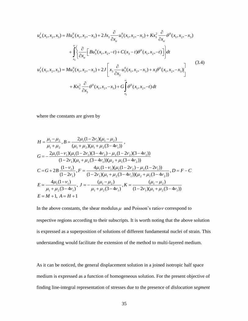
and for material points in region 1, positive values of 3x ,

35

3

0 0 2 0

1 2 3 1 2 3 3 3 1 2 3 3 1 2 3

0 0

3 1 2 3 1 2

0 0 0

3 1 2 3 3 1 2 3 3 3 1 2 3 3 1 2 3

3

( , , ) ( , , ) 2 ( , , ) ( , , )

( , , ) ( ) ( , , )

( , , ) ( , , ) 2 ( , , ) ( , , )

I

x

I

u x x x Hu x x x Jx u x x x Kx x x xx x

Bu x x t C x t x x t dtx

u x x x Mu x x x J x u x x x x x x xx

3

2 0 0

3 1 2 3 1 2

3

( , , ) ( , , )

x

Kx x x x G x x t dtx

(3.4)

where the constants are given by

1 2 1 1 1 2

1 2 1 2 1 2 1

1 1 1 1 2 2 2 1

1 1 2 1 2 1 2

1 1 1 1 2 2 1

1 1 1

2 (1 2 )( ), ,

( )( (3 4 ))

2 (1 )( (1 2 )(3 4 ) (1 2 )(3 4 ))

(1 2 )( (3 4 ))( (3 4 ))

(1 ) 4 (1 )( (1 2 ) (1 2 ))2 ,

(1 2 ) (1 2 )(

H B

G

C G B F

2 1 2 1 2

1 1 1 2 1 2

1 2 1 1 2 1 1 1 2 1

,(3 4 ))( (3 4 ))

4 (1 ) ( ) ( ), ,

(3 4 ) (3 4 ) (1 2 )( (3 4 ))

1, 1

D F C

E J K

E M A H

In the above constants, the shear modulus and Poisson‟s ratio correspond to

respective regions according to their subscripts. It is worth noting that the above solution

is expressed as a superposition of solutions of different fundamental nuclei of strain. This

understanding would facilitate the extension of the method to multi-layered medium.

As it can be noticed, the general displacement solution in a joined isotropic half space

medium is expressed as a function of homogeneous solution. For the present objective of

finding line-integral representation of stresses due to the presence of dislocation segment

36

in joined isotropic half-spaces, it would be appropriate to express the homogeneous

solution for such a case using Mura‟s line integral expression.

According to Mura‟s formulation(Mura 1987), the displacement gradient due to a

dislocation segment in a homogeneous infinite medium can be expressed as a line

integral over the dislocation line as given by

0

, 1 2 3 , 1 1 2 2 3 3( , , ) ( , , )j qi jnh pqmn ip m hu x x x C G x x x x x x b dl (3.5)

where , ,b are permutation tensor, Burgers vector and line sense respectively and

1 1 2 2 3 3 , 1 1 2 2 3 3

1 3

1

5

( , , ) ( , , )

( ) ( ) ( )1(1 2 )

8 (1 )

( )( )( )3

qmni pqmn ip

ni m m im n n mn i i

m m n n i i

CG x x x x x x C G x x x x x x

x x x x x x

R

x x x x x x

R

(3.6)

with 2 2 2

1 1 2 2 3 3( ) ( ) ( )R x x x x x x

Using the line integral expression for the displacement gradient in infinite homogeneous

medium given by (3.5)-(3.6) and the general displacement solution given by (3.3)-(3.4),

the line integral expressions for displacement gradients can be derived. Before going

further, it is very important to note that, in region 2, the derivation would yield a

complete solution for displacement gradient, whereas in region 1, the expressions

37

represent only the image displacement gradient. To illustrate the method, let us consider

equation (3.1) and substitute (3.5) to yield

3

3

,

0

1 2 3 1 2 3 3 , 1 1 2 2 3

3 1 1 2 2 3

( , , ) ( , , ) ( , , )

( ) ( , , )

q

q

x

II

nh pqmn p m h

x

jnh pqmn jp m h

u x x x Au x x x B C G x x x x t x b dl dt

Ct Dx C G x x x x t x b dl dt

(3.7)

The order of integration can be interchanged as the domains of integration are disjoint.

Thus, the above expression can be rewritten as

3

3

,

3

,

0

1 2 3 1 2 3 3 , 1 1 2 2 3

1 1 2 2 3

3 1 1 2 2 3

( , , ) ( , , ) ( , , )

( , , )

( , , )

q

q

q

x

II

nh pqmn p m h

x

jnh pqmn jp m h

x

jnh pqmn jp

u x x x Au x x x B C G x x x x t x dt b dl

C t C G x x x x t x dt b dl

Dx C G x x x x t x dt

m hb dl

(3.8)

The integrals inside the parenthesis are convergent and can be evaluated analytically.

(This was done using Mathematica). As a result the above expression can be written as

0

1 2 3 1 2 3 3 1 1 2 2 3 3

1 1 2 2 3 3

3 1 1 2 2 3 3

( , , ) ( , , ) ( , , )

( , , )

( , , )

II II

nh mn m h

II

jnh mnj m h

II

jnh mnj m h

u x x x Au x x x B IG x x x x x x b dl

C IGT x x x x x x b dl

Dx IGS x x x x x x b dl

(3.9)

where

38

3

1 1 2 2 3 3 1 1 2 2 3( , , , , , ) ( , , )

x

II

mni mniIG x x x x x x CG x x x x t x dt

(3.10.1)

3

,1 1 2 2 3 3 1 1 2 2 3( , , , , , ) ( , , )

x

II

mnj mnjIGT x x x x x x t CG x x x x t x dt

(3.10.2)

3

,1 1 2 2 3 3 1 1 2 2 3( , , , , , ) ( , , )

x

II

mnj mnjIGS x x x x x x CG x x x x t x dt

(3.10.3)

Furthermore, upon taking the spatial derivative of equation (3.9) and after expressing the

first term A 0

,ku in an integral form using Mura‟s formula, one can express the

displacement gradient as follows

,

, 1 2 3 1 1 2 2 3 3

1 1 2 2 3 3 3 ,

3 , 3

( , , ) ( , , , , , )

( , , , , , )

k

k k

k

II II

k mh m hl

II II II

k mh knh mn nh mn jnh mnj

II II

jnh mnj k jnh mnj

u x x x K x x x x x x b dl

K x x x x x x A CG B IG C IGT

D x IGS IGS

(3.11)

Similarly, all other components of displacement gradient can be derived and are given as

follows.

Region 2

3, 1 1 2 2 3 3

1 1 2 2 3 3 3 3

3 , ,

( , , , , , )

( , , , , , )

k

k k

II II

kmh m hl

II

kmh knh mn k jnh mnj

II

jnh mnj jnh mnj

u S x x x x x x b dl

S x x x x x x E CG F CG

Fx CG G IG

(3.12)

Region 1

39

, ,

,

, 1 1 2 2 3 3

1 1 2 2 3 3

3 3, 3 3

2

3 3 3

3,

3 3

( , , , , , )

( , , , , , )

2

2

i

i

i

i

i

I I

i mh m hl

I

i mh inh mn

nh mn i nh mn

jnh mnj i jnh mnj

I

nh mn

I

jnh mnj i jnh mnj

u K x x x x x x b dl

K x x x x x x H CG

J x CG CG

K x CG x CG

B IG

C x IGS IGS

,i

I

I

jnh mnjIGT

(3.13)

,

,

,3 ,3

3, 1 1 2 2 3 3

1 1 2 2 3 3 3 3 3 3

3 3 3 3

3

2

3 3 3

,

( , , , , , )

( , , , , , ) 2

2

i

i

i

i

i

I I

imh m hl

I

imh inh mn nh mn

i nh mn jnh mnj

i jnh mnj

jnh mnj i jnh mnj

I

jnh mnj

u S x x x x x x b dl

S x x x x x x M CG J x CG

CG x CG

CG

K x CG x CG

G IG

(3.14)

1 3

1

i

otherwise

where the tensors IIG , IIGS and IIGT in region 1 are defined in a similar way as

3

1 1 2 2 3 3 1 1 2 2 3( , , , , , ) ( , , )I

mni mni

x

IG x x x x x x CG x x x x t x dt

(3.15.1)

,

3

1 1 2 2 3 3 1 1 2 2 3( , , , , , ) ( , , )I

mnj mnj

x

IGS x x x x x x CG x x x x t x dt

(3.15.2)

40

,

3

1 1 2 2 3 3 1 1 2 2 3( , , , , , ) ( , , )I

mnj mnj

x

IGT x x x x x x t CG x x x x t x dt

(3.15.3)

The analytical expressions of all the components of the tensors

, , , ,I I I II IIIG IGS IGT IG IGS and IIIGT have been derived using Mathematica, a few of

these expression are given in Appendix 3.A, a complete list in the form of FORTRAN 90

subroutines can be downloaded from the site

http://www.cmm.wsu.edu/Downloads/Downloads.html

With the displacement gradient fields derived in both regions, the total stress field can

also be derived using Hooke‟s law and can be expressed in the following form:

Region 1

1 1

, 1 , ,

1

2

1 2 p j i

H I H I I I

ij ij ij ij p ij i ju u u

(3.16)

Region 2

,

2 22 , ,

2

2

(1 2 ) p j j

II II II II

ij ij p ij i iσ σ u u u

(3.17)

where H

ij denotes the solution in homogeneous medium with material properties of

region 1.

http://www.cmm.wsu.edu/Downloads/Downloads.html

41

3.2.2) Dislocation segment

Using the derived line integral expressions over the dislocation line, one can compute the

stress field due to a dislocation segment by employing a coordinate transformation along

the dislocation line.

For integration of the above integrals over any dislocation segment in an arbitrary

orientation, the coordinate system along the dislocation is employed. The origin of this

coordinate system is always at the center of the dislocation segment with positive

direction along the dislocation line sense. The mapping of this coordinate system onto the

three dimensional Cartesian coordinate system is given by (see Figure 3.2)

1 1

1 2

1 3

2

2

2

lx x

ly y

lz z

(3.18)

where is the dislocation line sense vector.

It is worth noting that the above expressions can be easily extended to continuous

distribution of dislocations by noting that the dislocation density is defined as

hm m hdV b dl (3.19)

42

The line integral expressions derived above can also be used to compute the stress field

of any arbitrary Voltera dislocation, or Somgliani dislocation with Burgers varying along

the dislocation line.

3.3. Infinite edge dislocation

In this section, the displacement gradient and, in turn, the stress field expressions due to

an infinite edge dislocation are derived by analytically integrating over the dislocation

line from to for various cases and compared with the existing analytical solutions

found in the literature. It is worth noting that the particular solutions presented below are

degenerated from the general line integral expressions for a dislocation segment derived

above.

3.3.1) Isotropic joined half space with bonded interface

Using the above line integral expressions, the analytical expressions for the displacement

gradient in equations (3.16) and (3.17) due to an infinite edge dislocation with its Burgers

vector perpendicular to the perfectly bonded interface are derived to yield the following.

For positive values of 3x , that is in region 1,

43

2 2 2

1 1 3 3 1 1 3 31, 2 2 21

1 1 3 3

2 2 2

1 1 3 3 3 3 1 1 3 33 2 2 3

1 1 3 3

2 1 1 1 13

2( )( 2 ( ) 3 (( ) ( ) ))

3(( ) ( ) )

4( )( )(4 ( ) 3 (( ) ( ) ))2

3(( ) ( ) )

8 ( )(( )

I x x B x x A x x x xu H

x x x x

x x x x B x x A x x x xJx

x x x x

A x x x xKx

2 2

3 3

2 2 3

1 1 3 3

2 2

1 1 1 1 3 3

2 2 2

1 1 3 3

1 1

2 2

1 1 3 3

3( ) )

(( ) ( ) )

2( ) (3 2 )( ) (3 4 )( )

3(( ) ( ) )

4 ( )

( ) ( )

x x

x x x x

x x A B x x A B x xB

x x x x

A x xC

x x x x

(3.20)

2 2

1 1 3 3 1 13, 2 2 23

1 1 3 3

22

3 3 3 3 3 3 3 3 1 1

1 134 2

1 1 3 3 3 1 1 3 3 3 3

2

1 1 3

2( )((3 2 )( ) 3 ( ) )

3(( ) ( ) )

2 ( ) ( )( ) 3

2( )

3 22

3

I x x A B x x A x xu M

x x x x

B x x x x x x x x x x

x x

A x x x x x x x x x x xJ

x x x

32

3

2 22 2

1 1 3 3 1 1 3 3 3 3 1 1 3 3

322

1 1 3 3

1 1

22

1 1 3 3

8 3 2

4 ( )

x

A x x x x x x x x x x x x x xK

x x x x

A x xG

x x x x

(3.21)

44

2 2

3 3 3 3 1 1

3, 21 22

1 1 3 3

2 2 42 4

3 3 1 1 3 3 1 1 3 3

3 322

1 1 3 3

22

3 3 1 1 3 32

3 322

1 1 3 3

2 3 2 3

3

2 3 34

3

8 3

Ix x A B x x A x x

u M

x x x x

B x x x x x x A x x x xJx

x x x x

A x x x x x xKx

x x x x

3 3

22

1 1 3 3

4A x xG

x x x x

(3.22)

22

3 3 1 1 3 3

1, 23 22

1 1 3 3

2 2 22 2

3 3 1 1 3 3 3 3 1 1 3 3

2 2 42 4

3 3 3 3 3 1 1 1 1 3 3

322

1 1 3 3

2 3 2 3

3

2 3

2 3 3

4

3

8

Ix x A B x x A x x

u H

x x x x

x x x x x x B x x A x x x x

x B x x x x x x A x x x x

J

x x x x

A xK

34 2

3 1 1 3 3 3 1 1 3 3 3

322

1 1 3 3

2 2

3 3 3 3 1 13 3

2 22221 1 3 31 1 3 3

3 ( )

2 3 2 3 4

3

x x x x x x x x x x

x x x x

x x A B x x A x x A x xB C

x x x xx x x x

(3.23)

For negative values of 3x , that is in region 2, the displacement gradients are given by

45

2 2

1 1 3 3 1 1

1, 21 22

1 1 3 3

22

1 1 1 1 3 3

222

1 1 3 3

2 2 2

1 1 1 1 3 3 3 3

3222

1 1 3 3

2 3 2 3

3

2 3 2 3 4

3

4 3 4 8

IIx x A B x x A x x

u A

x x x x

x x A B x x A B x xB

x x x x

A x x x x x x x x AC Dx

x x x x

1 1 3 3

222

1 1 3 3

x x x x

x x x x

(3.24)

2 2

1 1 3 3 1 1

3 2,3 22

1 1 3 3

2 2 2

1 1 1 1 3 31 1

2 2222

1 1 3 31 1 3 3

2 3 2 3

3

4 4

IIx x A B x x A x x

u E

x x x x

A x x x x x x A x xF G

x x x xx x x x

(3.25)

22

3 3 1 1 3 3

1, 23 22

1 1 3 3

2 2

3 3 3 3 1 1

222

1 1 3 3

22

3 1 1 3 3

222

1 1 3 3

2

3 3 3 3 3

2 3 2 3

3

2 3 2 3

3

4

4 2

IIx x A B x x A x x

u A

x x x x

x x A B x x A x xB

x x x x

A x x x x xC

x x x x

A x x x x xD

2

1 1

222

1 1 3 3

x x

x x x x

(3.26)

46

2 2

3 3 3 3 1 1

3, 21 22

1 1 3 3

2 2

3 3 3 1 13 3

2 2222

1 1 3 31 1 3 3

2 3 2 3

3

4 4

IIx x A B x x A x x

u E

x x x x

A x x x x x A x xF G

x x x xx x x x

(3.27)

where

1

1 1

(1 2 ) 3,

8 1 8 1A B

The expressions above when combined with equations (3.16) and (3.17) along with the

homogenous solution, which can be found in (Hirth and Lothe 1982), yield the complete

stress field in both regions. Subtracting the homogenous solution from both equations

(3.16) and (3.17) yields the image stress part which can then be compared with the exact

solution provided by (Head 1953a).

For the purpose of comparison, a bi-material medium with Cu (shear modulus, 1 equal

to 54.6GPa) as region 1 and Ni (shear modulus, 2 equal to 94.7GPa) as region 2 is

considered with an infinite edge dislocation 5 units of Cu Burgers vector magnitude away

from the interface is considered. In all the figures discussed below, the shear stress

component along the ordinate is normalized by shear modulus of Cu (region 1), and

along the abscissa the distance from the interface (located at the origin) is normalized

with the magnitude of the Burgers vector of Cu.

47

Typical results of shear stress component are shown in Figure 3.3. It is evident from the

shear stress field comparison that our analytical solution, although is in different

algebraic form, is identical to that derived by (Head 1953a). As the dislocation is in

softer medium, the presence of stiffer medium near it exerts an image force which repels

the dislocation further away from the interface and into the softer medium.

3.3.2) Isotropic half space with traction-free boundary

The second particular solution considered is that of an infinite edge dislocation in an

isotropic Cu half space with Burgers vector perpendicular to traction free boundary. The

edge dislocation is 5 units of Cu Burgers vector magnitude away from the free boundary.

The displacement gradient and in turn the stress expressions for this case can be easily

deduced by equating 2 to zero. A typical comparison of our analytical solution for the

image shear stress component is made with (Head 1953a) solution which shows perfect

agreement as can be seen from Figure 3.4.

As can be deduced from Figure 3.4, as the boundary of the half space is a traction free

surface, the shear stress is negative which results in Peach-Koehler force attracting the

edge dislocation towards the surface as expected.

48

3.3.3) Isotropic half space with rigid boundary

As another extreme case, the solution of an infinite edge dislocation in isotropic Cu half

space with Burgers vector perpendicular to the rigid boundary is considered. For this

particular case, the solution can be deduced when 2 tends to infinity. It can be noticed

that the constants B, C and G vanish in this limit. The image shear stress component

shown in Figure 5.5 implies that the dislocation is repelled by the rigid boundary as

expected.

3.3.4) Interface dislocation

Finally, we consider the solution of an infinite edge dislocation at the perfectly bonded

interface with its Burgers vector perpendicular to the interface which can be obtained by

equation 3x to zero. The image shear stress plot for this case is shown in Figure 5.6.

3.3.5) Circular dislocation loop

In this sub-section, to illustrate the scope of the method, we consider prismatic circular

loop in the plane parallel to the interface 5 units of Cu Burgers vector magnitude away

from the Cu/Ni interface into the Cu medium. The circular loop is discretized into

collection of straight dislocation segments and the stress field is computed by numerically

integrating the above derived line integral expressions along all the straight dislocation

segments. The image shear stress component plotted along a line parallel to 3x axis and 5

49

units of Cu Burgers vector magnitude away from the origin in the 1x direction is shown in

the Figure 5.7(a) for different refinement in discretization of circular loop. As it can be

noticed from the plot, the solution converges upon mesh refinement of the dislocation

loop.

We have also considered a glide circular loop in the plane parallel to the interface 5 units

of Cu Burgers vector magnitude away from the Cu/Ni interface into the Cu medium. By

numerically integrating the line integral expressions along all the dislocation segments,

the stress field and , in turn , the Peach-Koehler force acting on the loop only due to the

presence of a different material is computed and shown as a vector plot in the Figure

5.7(b). As it can be seen from the plot, the equilibrium of the loop is disturbed by the

effect of image stresses due to the presence of a different material.

3.4. Conclusions

A method is presented to derive line integral expressions for stress and image

displacement fields due a dislocation segment in joined 3D half space medium with

perfectly bonded interface. The methodology is based on combining Walpole‟s general

solution, which is expressed in terms of homogeneous solution, and Mura‟s integral

formula for a dislocation segment in homogeneous medium. The line integral expressions

can be solved analytically, providing exact solutions. A particular case of an edge

dislocation with its Burgers vector perpendicular to the interface is considered and

analytical expressions are derived which are then compared with Head‟s solution. The

50

solutions of an edge dislocation near a traction free and rigid boundary of a half space

and at the interface of joined half space are also computed as special degenerate cases

and the stress fields are shown.

Although Walpole‟s general solution is not derived from the method of images by

superposition of solutions of appropriate nuclei of strain, the separation of the solution in

terms of two components, homogenous and image components, and expressing the image

part in terms of the homogeneous solution enabled the derivation of the line integral

expressions for the dislocation segment. A general extension of such method for multi-

layered medium can be possible by expressing the solutions of fundamental nuclei of

strain in joined half space in terms of homogenous solutions.

Acknowledgment

This work was supported by the Division of Materials Science and Engineering, Office of

Basic Energy Science at the U.S. Department of Energy under grant number DE-FG02-

07ER4635.

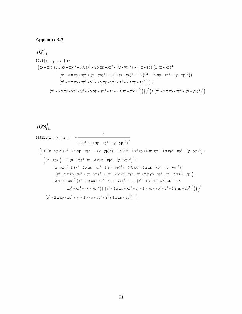
51

Appendix 3.A

111

IIG

111

IIGS

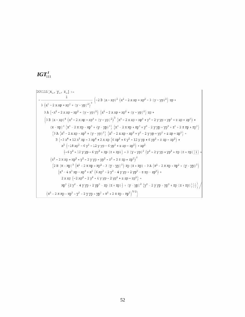
52

111

IIGT

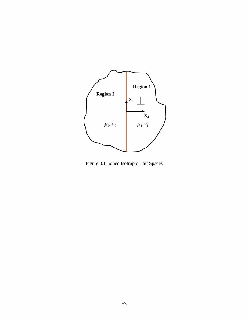
53

Figure 3.1 Joined Isotropic Half Spaces

X3

X1

Region 1

Region 2

1 1, 2 2,

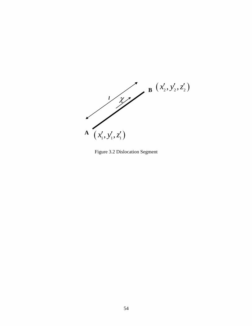
54

Figure 3.2 Dislocation Segment

A

l

B

1 1 1, ,x y z

2 2 2, ,x y z

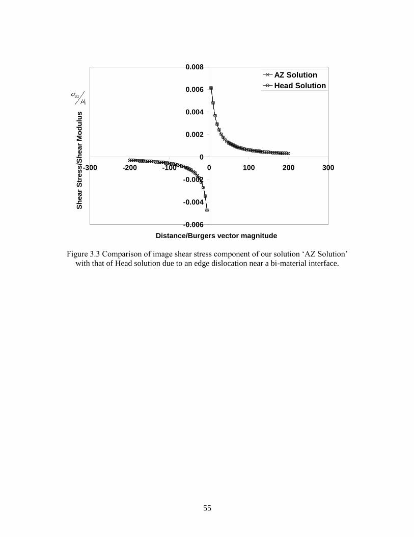
55

-0.006

-0.004

-0.002

0

0.002

0.004

0.006

0.008

-300 -200 -100 0 100 200 300

Distance/Burgers vector magnitude

Sh

ea

r S

tre

ss

/Sh

ea

r M

od

ulu

sAZ Solution

Head Solution

Figure 3.3 Comparison of image shear stress component of our solution „AZ Solution‟

with that of Head solution due to an edge dislocation near a bi-material interface.

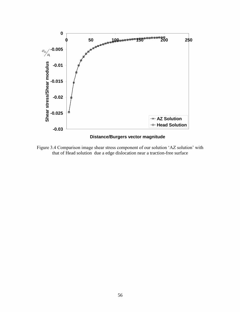
56

-0.03

-0.025

-0.02

-0.015

-0.01

-0.005

0

0 50 100 150 200 250


Sh

ear

str

ess/S

hear

mo

du

lus

AZ Solution

Head Solution

Figure 3.4 Comparison image shear stress component of our solution „AZ solution‟ with

that of Head solution due a edge dislocation near a traction-free surface

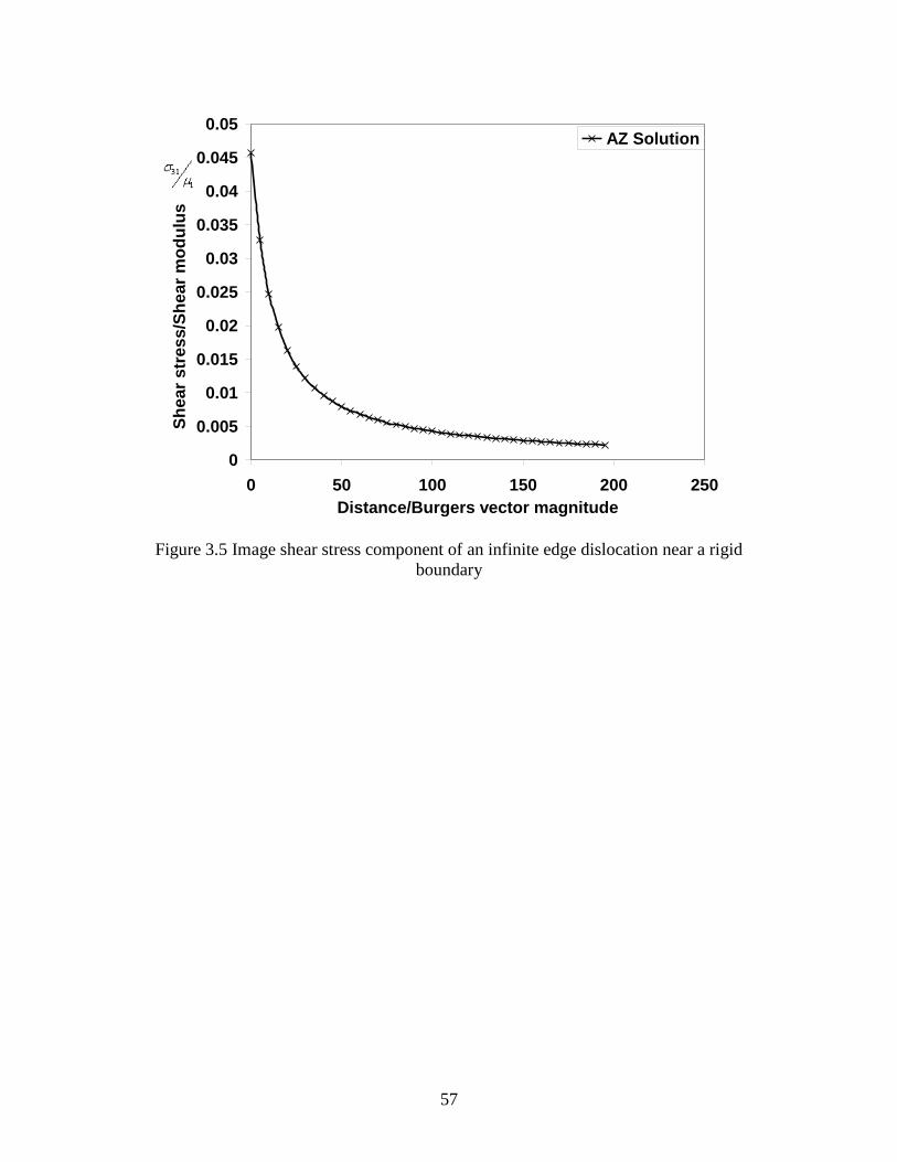
57

0

0.005

0.01

0.015

0.02

0.025

0.03

0.035

0.04

0.045

0.05

0 50 100 150 200 250


Sh

ear

str

ess/S

hear

mo

du

lus

AZ Solution

Figure 3.5 Image shear stress component of an infinite edge dislocation near a rigid

boundary

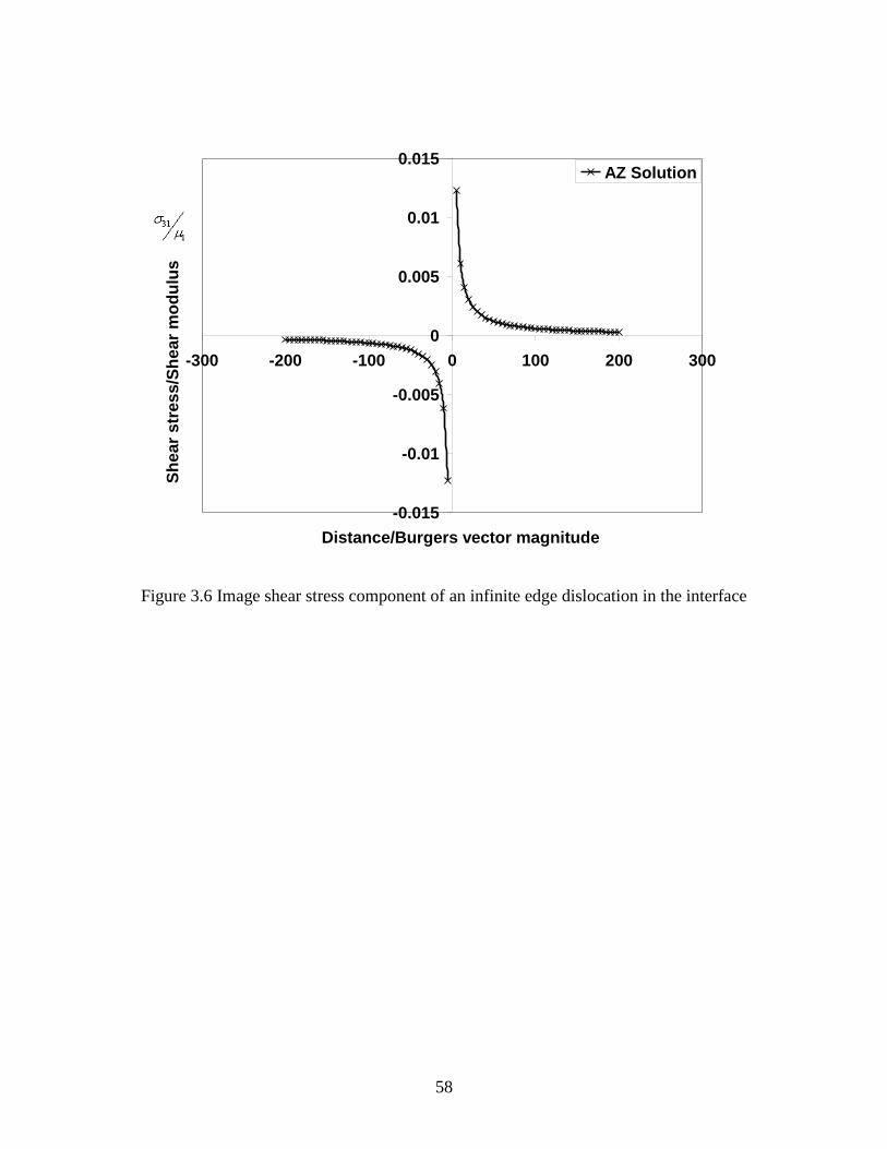
58

Figure 3.6 Image shear stress component of an infinite edge dislocation in the interface

-0.015

-0.01

-0.005

0

0.005

0.01

0.015

-300 -200 -100 0 100 200 300


Sh

ear

str

es

s/S

he

ar

mo

du

lus

AZ Solution

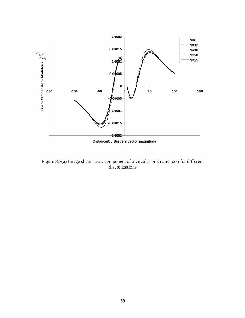
59

Figure 3.7(a) Image shear stress component of a circular prismatic loop for different

discretizations

31

1

-0.0002

-0.00015

-0.0001

-0.00005

0

0.00005

0.0001

0.00015

0.0002

-150 -100 -50 0 50 100 150

Distance/Cu Burgers vector magnitude

Sh

ear

Str

es

s/S

hear

Mo

du

lou

sN=8

N=12

N=16

N=20

N=25

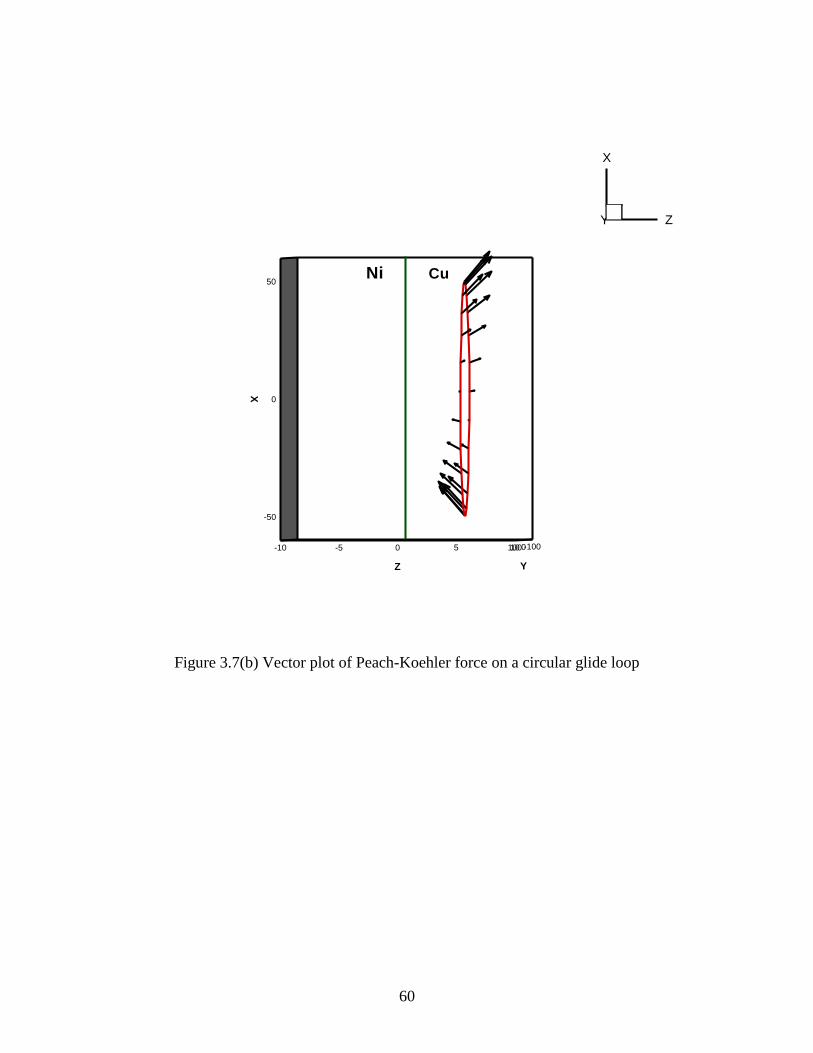
60

Figure 3.7(b) Vector plot of Peach-Koehler force on a circular glide loop

X

-50

0

50

Y

-1000100

Z

-10 -5 0 5 10

X

Y Z

CuNi

61

International Journal of Mechanics and Materials in Design, Vol. 4, pp. 399-406, 2008

CHAPTER FOUR: DISLOCATION INTERACTIONS WITH TILT WALLS

S Akarapua*

, H Zbiba

a

School of Mechanical and Materials Engineering

Washington State University, Pullman, WA-99164

Abstract

The flow of plastic deformation in polycrystalline materials can be due to activation of

sources in adjacent grains due to the effect of pile up dislocations against the grain

boundary and also through the transmission of dislocations across the grain boundary. In

this paper, we focus on these two issues by studying the evolution of resolved shear stress

as a result of pile up dislocations against the boundary and understanding the basic

phenomena of dislocation transmission through grain boundary. We also investigated the

relaxed structures a grain boundary acquires after the process of dislocation transmission.

4.1 Introduction

The polycrystalline deformation of material can be explained on the basis of

phenomenological knowledge of single crystal deformation properties. The single crystal

deformation can be studied by classical phenomenological theory which does not include

size effects or by improved gradient plasticity theories which have shear strain gradients

as internal variable to better describe size effects inherent in plasticity (Zbib and Aifantis

1989d; Zbib and Aifantis 1989c; Zbib and Aifantis 1989b; Fleck and Hutchinson 2001).

In the top-down approach, these theories are improved by employing internal variables

62

derived from the microscopic mechanisms (Gurtin 2000; Mesarovic 2005b; Shizwa and

Zbib 1999). The single crystal deformation is also studied in a bottom-up approach using

atomistic simulations (Horstemeyer and Baskes 1999). In all the polycrystalline models

developed from the single crystal deformation using Taylor-type assumptions (Asaro and

Needleman 1985; Hutchinson 1976; Kalidindi et al. 1992), Sachs-type assumptions

(Leffers and Van Houtte 1989) and using self-consistent approaches (Molinari et al.

1987) have a single crystal as their representative volume element and as a result are

deficient of grain boundary effect into the theory. In this paper, we study the dislocation

interactions with grain boundary to point out the importance of these effects in the

polycrystalline theories.

In polycrystalline materials, plastic deformation is caused by flow of plasticity across

several grains. The nature of flow of plastic deformation from one grain to another is

mainly dependent on the resistance of the grain boundary. Depending on the strength of

the grain boundary, dislocations can pile-up against it or shear the boundary and transmit

into the adjacent grain. In the former case, the pile-up of dislocations against the grain

boundary would activate sources in the neighboring grains thus enabling the flow of

plasticity across many grains. In this paper, we mainly focus on these two issues: Firstly,

the effect of pile-up dislocations against the grain boundary on the plasticity in the

adjacent grains and secondly, the basic phenomena of dislocation transmission across the

grain boundary and the relaxed structure it acquires after accommodating the plastic

incompatibility. In section 4.2, we study the effect of pile-up of dislocations against a

pure tilt wall in the adjacent grain as a function of misorientation across the boundary. In

63

section 4.3, we study the basic phenomenon of dislocation transmission and followed by

the methodology of computing the long-range stress field of dislocation configuration in

section 4.4. In section 4.5, we propose and explain the relaxed configurations the grain

boundary stabilizes to after transmission of dislocations and followed by summary.

4.2 Effect of Pile-up dislocations

In this section, we consider the flow of plasticity to the adjacent grains through the

activation of sources caused by the piled up dislocations against the grain boundary.

Towards this end, we considered an infinite bi-crystal with pure tilt wall as the grain

boundary model as shown in the Figure 4.1(a) and studied the evolution of resolved shear

stress in grain B as the dislocations pile-up in grain A against the boundary. The effect of

pile-up dislocations in grain A on the stress field in grain B is a function of misorientation

across the grain boundary which is governed by the inter-dislocation spacing in the wall.

As shown in the Figure 4.1 (b), the resolved shear stress in the grain B is plotted as

function of slip in grain A for various misorientations across the boundary. The slip in

grain A is defined as

Slip = 2

1

N

i

i

xb

L

(4.1)

Where ix , L, b and N denote the position of dislocation, length of pile-up, burgers vector

and number of dislocations in the pile-up respectively.

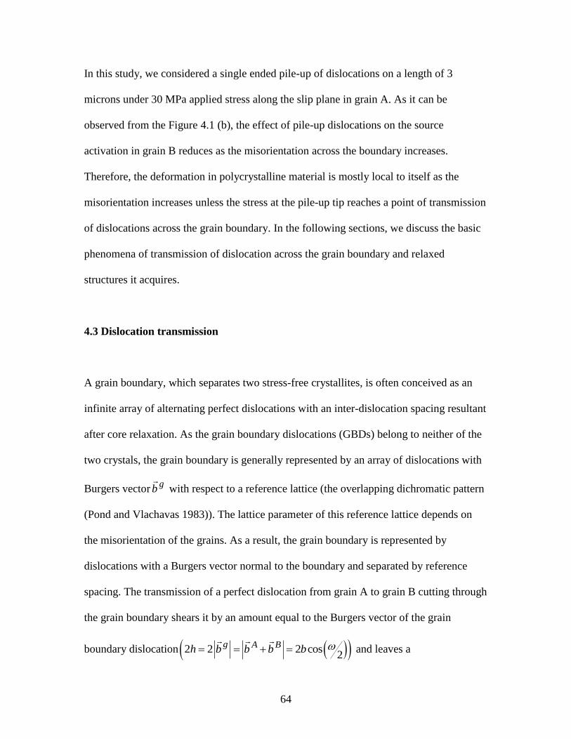
64

In this study, we considered a single ended pile-up of dislocations on a length of 3

microns under 30 MPa applied stress along the slip plane in grain A. As it can be

observed from the Figure 4.1 (b), the effect of pile-up dislocations on the source

activation in grain B reduces as the misorientation across the boundary increases.

Therefore, the deformation in polycrystalline material is mostly local to itself as the

misorientation increases unless the stress at the pile-up tip reaches a point of transmission

of dislocations across the grain boundary. In the following sections, we discuss the basic

phenomena of transmission of dislocation across the grain boundary and relaxed

structures it acquires.

4.3 Dislocation transmission

A grain boundary, which separates two stress-free crystallites, is often conceived as an

infinite array of alternating perfect dislocations with an inter-dislocation spacing resultant

after core relaxation. As the grain boundary dislocations (GBDs) belong to neither of the

two crystals, the grain boundary is generally represented by an array of dislocations with

Burgers vectorg

b

with respect to a reference lattice (the overlapping dichromatic pattern

(Pond and Vlachavas 1983)). The lattice parameter of this reference lattice depends on

the misorientation of the grains. As a result, the grain boundary is represented by

dislocations with a Burgers vector normal to the boundary and separated by reference

spacing. The transmission of a perfect dislocation from grain A to grain B cutting through

the grain boundary shears it by an amount equal to the Burgers vector of the grain

boundary dislocation 2 2 2 cos2

g A Bh b b b b

and leaves a

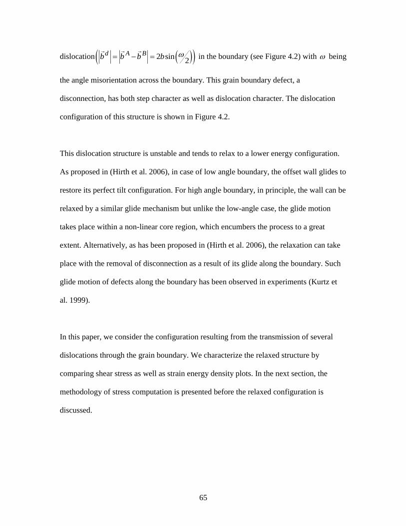
65

dislocation 2 sin2

d A Bb b b b

in the boundary (see Figure 4.2) with being

the angle misorientation across the boundary. This grain boundary defect, a

disconnection, has both step character as well as dislocation character. The dislocation

configuration of this structure is shown in Figure 4.2.

This dislocation structure is unstable and tends to relax to a lower energy configuration.

As proposed in (Hirth et al. 2006), in case of low angle boundary, the offset wall glides to

restore its perfect tilt configuration. For high angle boundary, in principle, the wall can be

relaxed by a similar glide mechanism but unlike the low-angle case, the glide motion

takes place within a non-linear core region, which encumbers the process to a great

extent. Alternatively, as has been proposed in (Hirth et al. 2006), the relaxation can take

place with the removal of disconnection as a result of its glide along the boundary. Such

glide motion of defects along the boundary has been observed in experiments (Kurtz et

al. 1999).

In this paper, we consider the configuration resulting from the transmission of several

dislocations through the grain boundary. We characterize the relaxed structure by

comparing shear stress as well as strain energy density plots. In the next section, the

methodology of stress computation is presented before the relaxed configuration is

discussed.

66

4.4. Stress computation method

Before going further into the discussion of long-range stress fields of concerned

dislocation configurations, we present a general methodology for finding the stress fields.

The long-range stress field of the dislocation is calculated using Mura‟s formula (Mura

1987), which is given by

,ij pqmnijkl lnh kp q hm

V

x C C G x x x dV

(4.2)

where kphm G,α,C,σ ιjκλιj , and lnhε denote the stress tensor at a material point x

, material

stiffness tensor, dislocation density tensor, Green‟s function and permutation tensor

respectively, and the subscript ,q indicates spatial derivative with respect to spatial

coordinate qx . We developed a computational algorithm to solve equation (4.2) for any

given anisotropic material stiffness tensor and dislocation density tensor. For isotropic

materials we use the following reduction:

, 3 5

11 2 3

8 1

n ni m mn imk n m ipqmn kp q

x x x x x xC G x

x x

(4.3)

in which x x x

and x x x

, with and being the Poisson ratio and Kroneker

delta function, respectively.

67

Thus, one can calculate the stress distribution of a collection of dislocations in an infinite

medium by numerically integrating (4.2) with an appropriate dislocation density tensor

which aptly represents the dislocation configuration and content. The long-range stress

field of a collection of discrete dislocations can be computed as the sum of the self stress

fields of each dislocation. A pure edge dislocation can be represented in terms of Dirac‟s

delta functions through the dislocation density tensor as

31 1 1 2b x x (4.4)

where 1b denotes the 1x component of Burgers vector.

The shear stress field of a finite edge dislocation wall as computed analytically was

compared with the numerical result obtained from Mura‟s formula to gain confidence in

the present methodology. We obtained the analytical results using the expressions for the

stress field of a pure edge dislocation given in (Hirth and Lothe 1982). As shown in

Figure 4.3, there is a good agreement with the analytical result.

The components of stress field of a disclination dipole are computed from the formulae

given in (Li 1972), which, in units of 2 1 , are given by

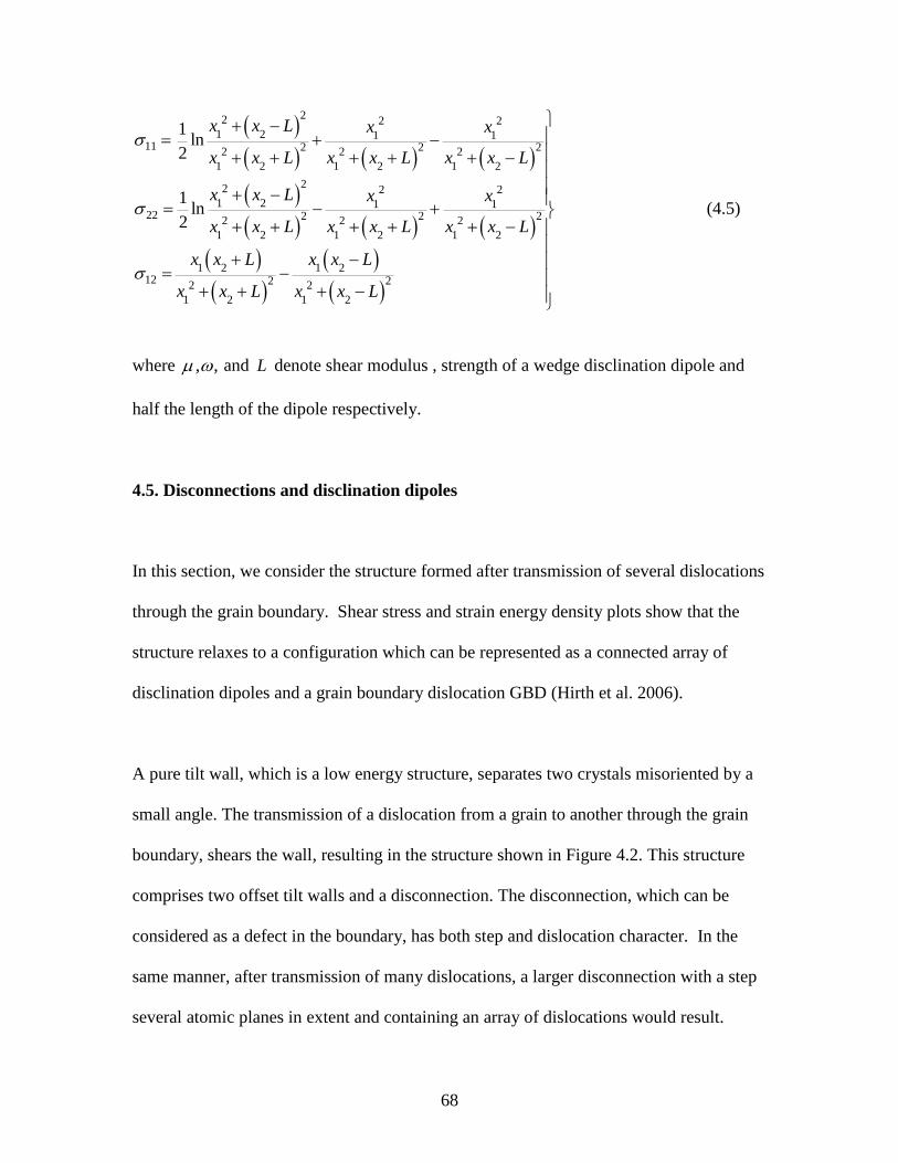
68

22 2 2

1 2 1 111 2 2 22 2 2

1 2 1 2 1 2

22 2 2

1 2 1 122 2 2 22 2 2

1 2 1 2 1 2

1 2 1 212 2 22 2

1 2 1 2

1ln

2

1ln

2

x x L x x

x x L x x L x x L

x x L x x

x x L x x L x x L

x x L x x L

x x L x x L

(4.5)

where , , and L denote shear modulus , strength of a wedge disclination dipole and

half the length of the dipole respectively.

4.5. Disconnections and disclination dipoles

In this section, we consider the structure formed after transmission of several dislocations

through the grain boundary. Shear stress and strain energy density plots show that the

structure relaxes to a configuration which can be represented as a connected array of

disclination dipoles and a grain boundary dislocation GBD (Hirth et al. 2006).

A pure tilt wall, which is a low energy structure, separates two crystals misoriented by a

small angle. The transmission of a dislocation from a grain to another through the grain

boundary, shears the wall, resulting in the structure shown in Figure 4.2. This structure

comprises two offset tilt walls and a disconnection. The disconnection, which can be

considered as a defect in the boundary, has both step and dislocation character. In the

same manner, after transmission of many dislocations, a larger disconnection with a step

several atomic planes in extent and containing an array of dislocations would result.

69

Alternatively, an array of unit disconnections formed at various locations along the grain

boundary can possibly glide along the boundary to form the larger disconnection. This

structure, shown in Figure 4.4(b), with the array of dislocations lumped into a dislocation

at the origin can be considered as a general configuration. The long-range stresses are

unaltered by lumping according to St. Venant‟s principle. In this particular study, we

consider an offset of height equal to 4D (D, being the inter-dislocation spacing) with an

array of m 4 gD b

dislocations, with m being the number of transmitted dislocations

needed to produce a step of height 4D. This general configuration reduces to the structure

resulting after a dislocation transmission in the limit as 4D h (see Figure 4.2 and

4.4(b)). In the calculations, finite dislocation walls with lengths L>>D are considered

instead of infinite and semi-infinite walls for ease of computation of stress and energy

density. The local fields are the same in all of these cases.

To confirm the fact that transmission of dislocations through a grain boundary results in

a higher energy structure, a comparison of shear stress and strain energy density was

made between the structures shown in Figure 4.4. The shear stress plot in Figure 4.5(a)

shows that the stresses are higher for the configuration in Figure 4.4(b) as compared with

the finite edge dislocation wall. The long-range stresses of both configurations, after a

distance approximately equal to the length of the wall, are almost equal, which conforms

to St. Venant‟s principle. The dislocation structure formed after transmission is also a

higher energy configuration as compared with the finite edge dislocation wall as can

observed from Figure 4.5(b).

70

Intuitively, one can argue that as the offset walls are separating two grains misoriented

with each other, the material in the offset region will undergo some local changes (e.g.

local lattice rotation) and relax into a dislocation structure that would preserve the

misorientation between the grains. For the dislocation configuration shown in Figure

4.4(b), the step portion of the larger disconnection relaxes to form a connecting branch to

the offset walls preserving the misorientation, which is indeed a lower energy structure.

The lattice planes of the connecting wall are orthogonal to that of the offset wall in order

to preserve the nature of rotation across the boundary (Hirth and Ballufi 1973).

In other words, the stresses of an offset disclination dipole should decrease upon

formation of disconnection comprising steps with right-angle bends because the shear

stress of an equal-armed right angle bend is zero at angle of 45°. Accordingly, the

resultant configuration after the relaxation of the disconnection portion of the dislocation

structure (see Figure 4.4 (b)) can be represented as a connected array of disclination

dipoles. The details of stress and energy plots are given in (Akarapu et al. 2008).

The general configuration after transmission of several dislocations through the boundary

with an offset of several atomic planes in extent, as shown in Figure 4.6(a), relaxes into a

connected array of disclination dipoles and a grain boundary dislocation as shown in

Figure 4.6(b). The energy of the structure is further reduced by splitting the grain

boundary dislocation into two at one-third positions from the origin as shown in Figure

4.6(c). The splitting of the grain boundary dislocation is terminated based on structural

considerations with the smallest Burgers vector belonging to the dichromatic pattern

71

(Pond and Vlachavas 1983). One can demonstrate the relaxation quantitatively by

comparing the strain energy density of the configurations shown in Figure 4.6(d). It can

be observed from the Figure 4.6(c) that there is a significant decrease in strain energy

density.

While relaxed the configuration of Figure 4.6 (c) has no long-range stresses, evidently

there remain local stresses near the defect. These remaining stresses can be reduced, or

in the limit, removed by local pileup-like rearrangements of both intrinsic GBDs in the

discontinuous tilt walls and of both intrinsic and extrinsic dislocations in the step. For a

step other than the right-angle steps considered here, the stresses would be longer range

and the rearrangements more complex. Consideration of the details of these

rearrangements is beyond the scope of the present work.

4.6 Summary

In summary, we have addressed the effect of pile-up dislocations against the grain

boundary and its influence in activating sources in the adjacent grains. We also studied

the basic phenomena of dislocation transmission and resulting configurations. The stress

analysis of dislocation configurations resulting from the transmission of dislocation

through a finite wall is discussed and their strain energies are compared. The results show

that the dislocation configuration resulting after the formation of an array of

disconnections relaxes into a connected array of disclination dipoles of equal strength and

a grain boundary dislocation. The relaxed array has no long-range stresses but has local

72

stresses that can only be removed by local rearrangements of dislocation spacings near

the defect.

Acknowledgement: The support from DOE under grant number DE-FG02-05ER25709

is gratefully acknowledged. The authors also wish to thank Dr. J.P. Hirth for all the

fruitful discussions we have had over the subject discussed in the paper and other related

subjects.

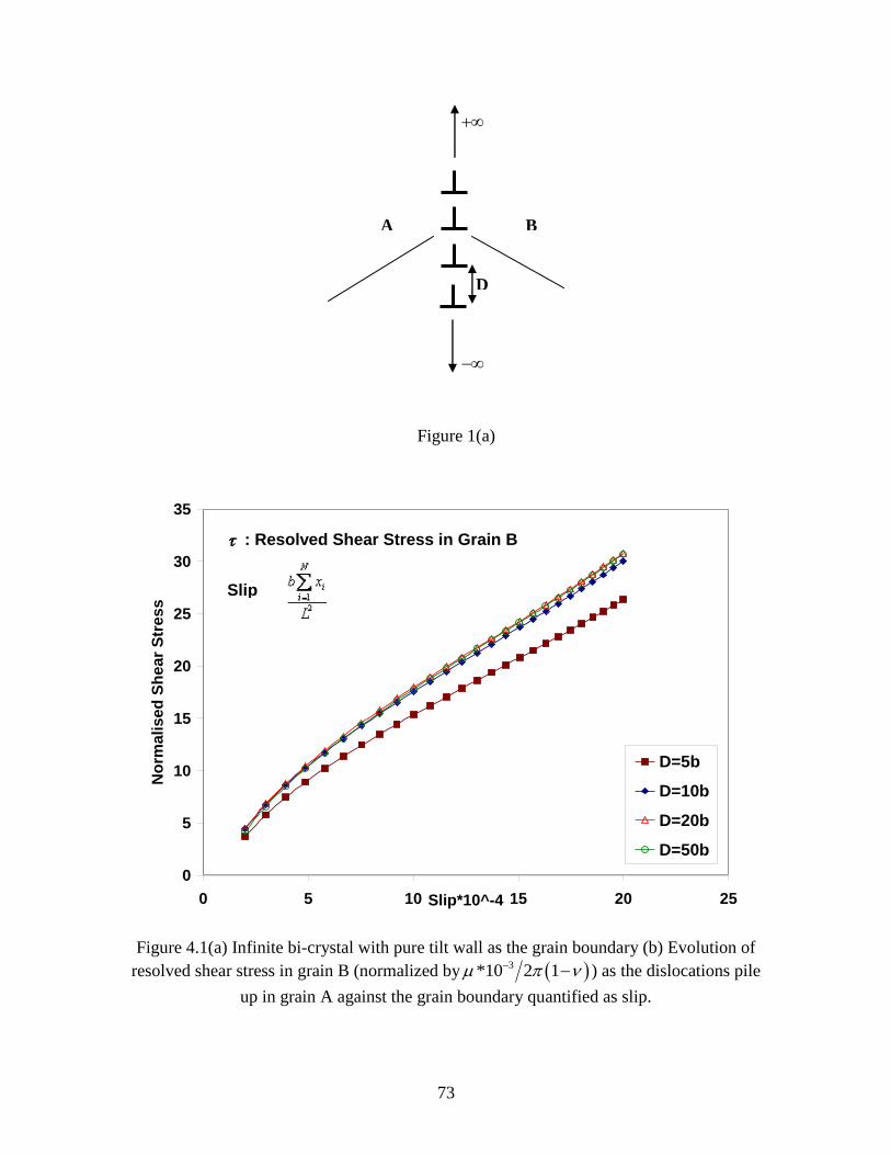
73

0

5

10

15

20

25

30

35

0 5 10 15 20 25Slip*10^-4

No

rmalised

Sh

ear

Str

ess

D=5b

D=10b

D=20b

D=50b

: Resolved Shear Stress in Grain B

Slip

Figure 4.1(a) Infinite bi-crystal with pure tilt wall as the grain boundary (b) Evolution of

resolved shear stress in grain B (normalized by 3*10 2 1 ) as the dislocations pile

up in grain A against the grain boundary quantified as slip.

Figure 1(a)

A B

D

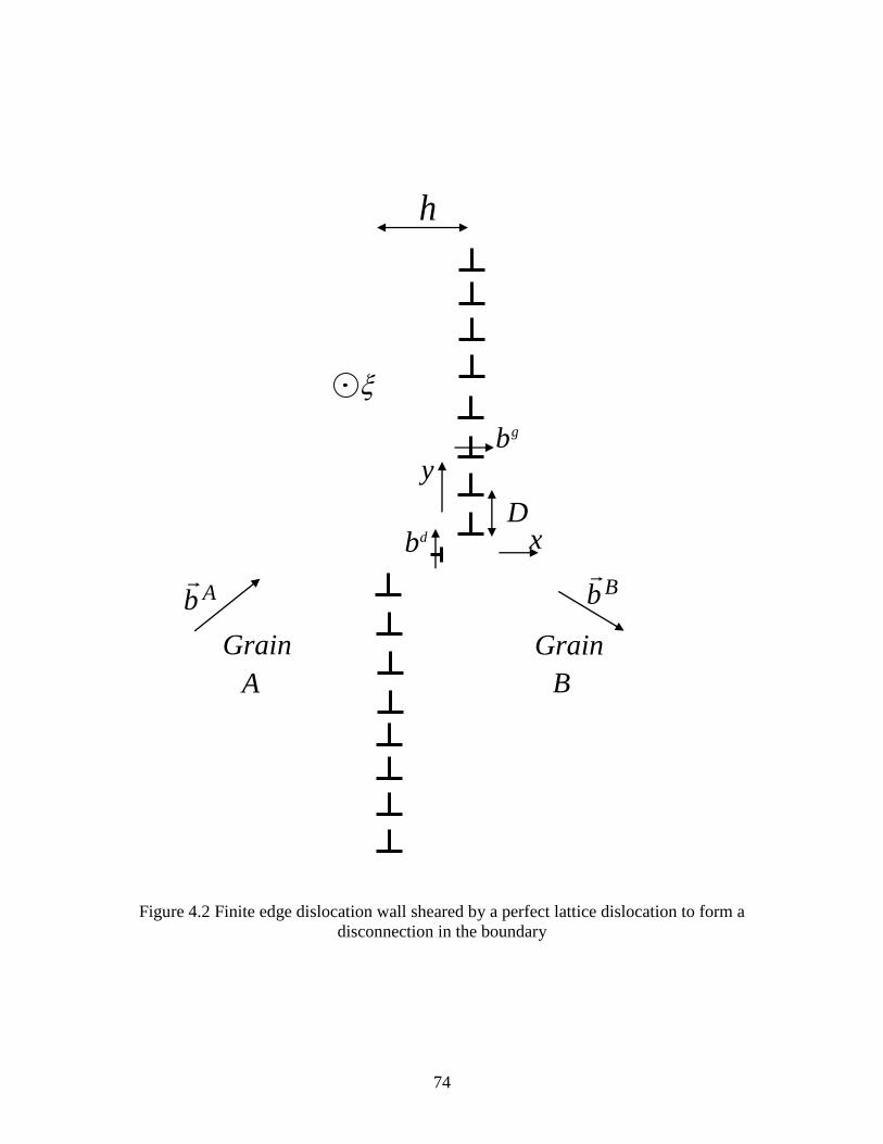
74

Figure 4.2 Finite edge dislocation wall sheared by a perfect lattice dislocation to form a

disconnection in the boundary

gb

x

y

D

h

db

Grain

A

Grain

B

Ab Bb

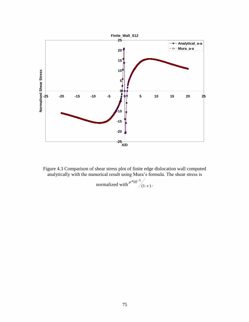
75

Finite_Wall_S12

-25

-20

-15

-10

-5

0

5

10

15

20

25

-25 -20 -15 -10 -5 0 5 10 15 20 25

X/D

No

rmali

sed

Sh

ear

Str

ess

Analytical_a-a

Mura_a-a

Figure 4.3 Comparison of shear stress plot of finite edge dislocation wall computed

analytically with the numerical result using Mura‟s formula. The shear stress is

normalized with3*10

(1 )

.

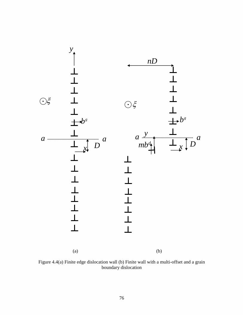
76

(a) (b)

Figure 4.4(a) Finite edge dislocation wall (b) Finite wall with a multi-offset and a grain

boundary dislocation

gb

x

y

Da a

gb

x

y

Da a

dmb

nD

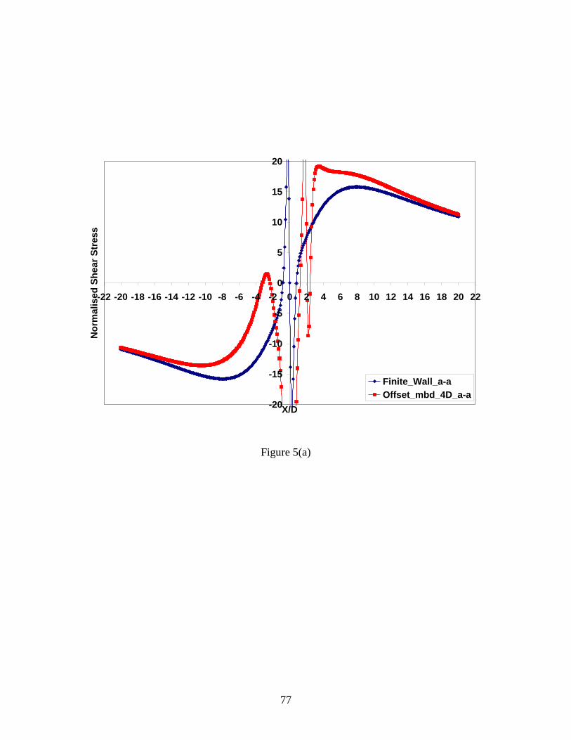
77

-20

-15

-10

-5

0

5

10

15

20

-22 -20 -18 -16 -14 -12 -10 -8 -6 -4 -2 0 2 4 6 8 10 12 14 16 18 20 22

X/D

No

rmalised

Sh

ear

Str

ess

Finite_Wall_a-a

Offset_mbd_4D_a-a

Figure 5(a)

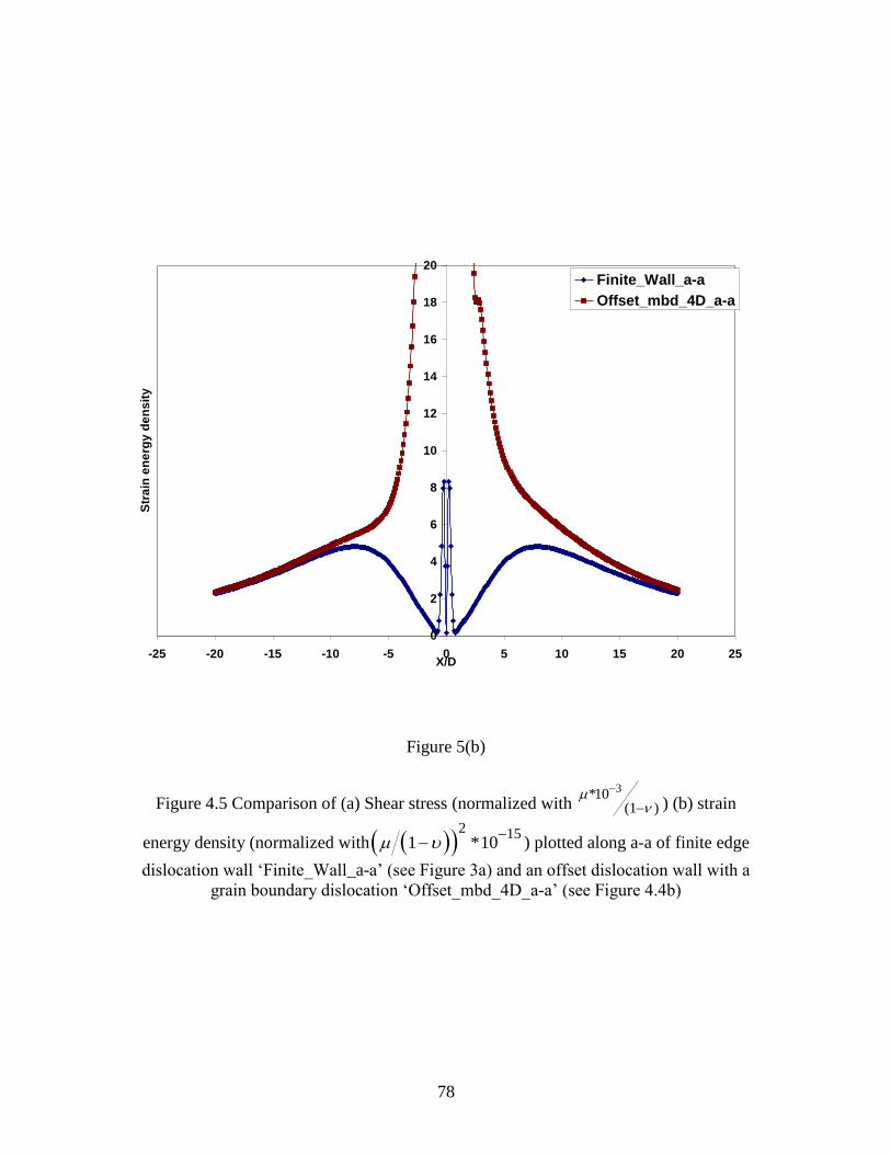
78

Figure 5(b)

Figure 4.5 Comparison of (a) Shear stress (normalized with 3*10

(1 )

) (b) strain

energy density (normalized with 2 15

1 *10

) plotted along a-a of finite edge

dislocation wall „Finite_Wall_a-a‟ (see Figure 3a) and an offset dislocation wall with a

grain boundary dislocation „Offset_mbd_4D_a-a‟ (see Figure 4.4b)

0

2

4

6

8

10

12

14

16

18

20

-25 -20 -15 -10 -5 0 5 10 15 20 25X/D

Str

ain

en

erg

y d

en

sit

y

Finite_Wall_a-a

Offset_mbd_4D_a-a

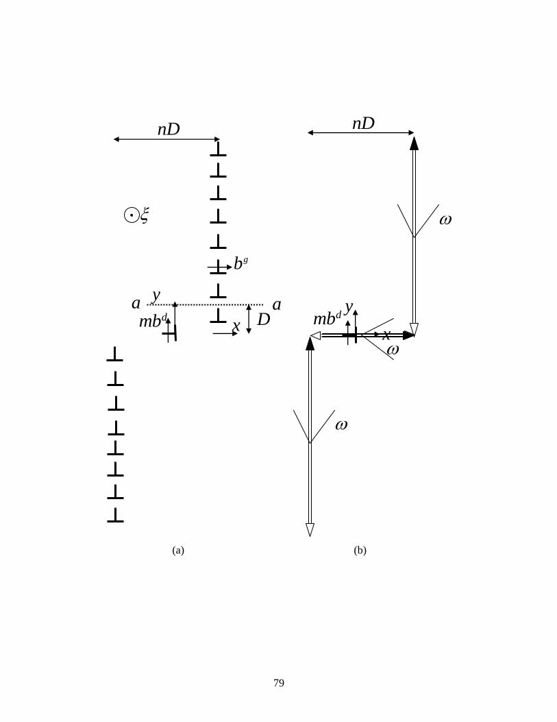
79

(a) (b)

x

y

nD

dmb

gb

x

y

Da a

dmb

nD

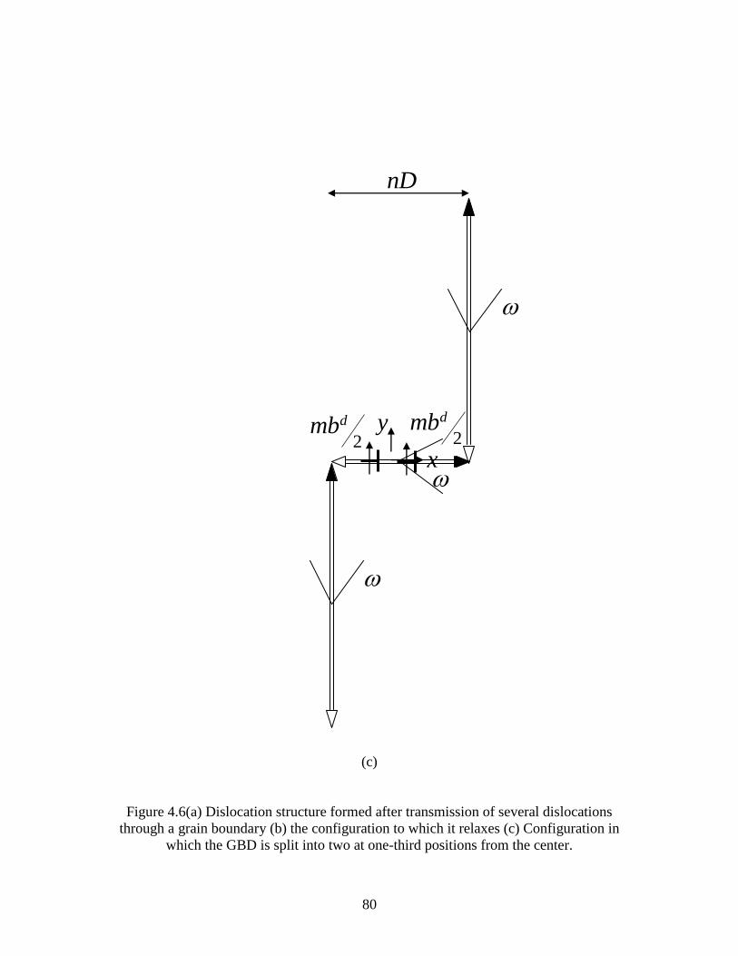
80

(c)

Figure 4.6(a) Dislocation structure formed after transmission of several dislocations

through a grain boundary (b) the configuration to which it relaxes (c) Configuration in

which the GBD is split into two at one-third positions from the center.

x

y

nD

2

dmb

2

dmb

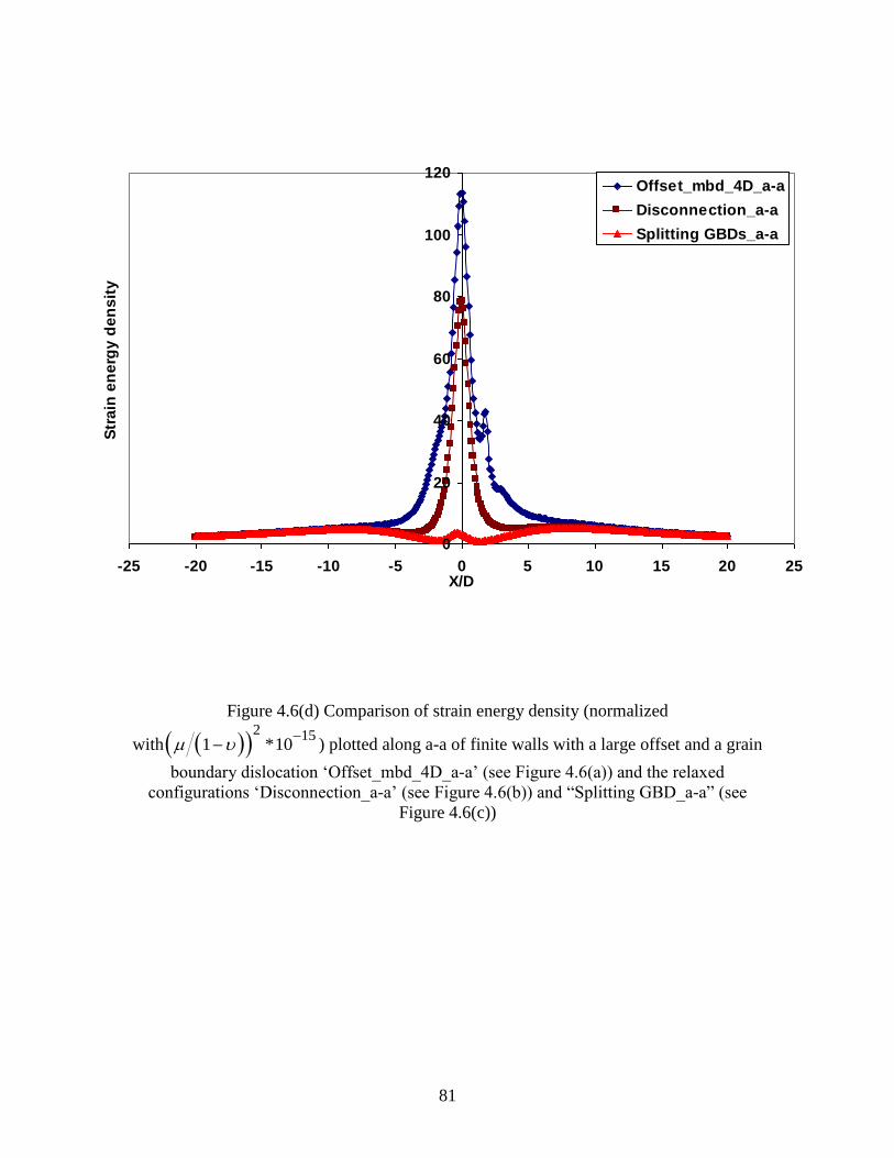
81

Figure 4.6(d) Comparison of strain energy density (normalized

with 2 15

1 *10

) plotted along a-a of finite walls with a large offset and a grain

boundary dislocation „Offset_mbd_4D_a-a‟ (see Figure 4.6(a)) and the relaxed

configurations „Disconnection_a-a‟ (see Figure 4.6(b)) and “Splitting GBD_a-a” (see

Figure 4.6(c))

0

20

40

60

80

100

120

-25 -20 -15 -10 -5 0 5 10 15 20 25X/D

Str

ain

en

erg

y d

en

sit

y

Offset_mbd_4D_a-a

Disconnection_a-a

Splitting GBDs_a-a

82

International Journal of Solids and Structures (Submitted)

CHAPTER FIVE: ENERGIES AND DISTRIBUTIONS OF DISLOCATIONS IN

STACKED PILE-UPS

Raghuraman Baskaran, Sreekanth Akarapu, Sinisa Dj. Mesarovic* & Hussein M. Zbib

School of Mechanical and Materials Engineering, Washington State University, Pullman,

WA 99164-2620

Abstract

To understand the kinematic and thermodynamic effects of representing discrete

dislocations as continuous distributions in their slip planes, we consider stacked double

ended pile-ups of edge and screw dislocations and compute their distributions and

microstructural energies, i.e., the elastic interaction energies of geometrically necessary

dislocations (GNDs).

In general, three kinds of representations of GNDs are used: discrete, semi-discrete, and,

continuous representation. The discrete representations are closest to reality. Therefore,

the corresponding solutions are considered exact. In the semi-discrete representation, the

discrete dislocations are smeared out into continuous planar distributions within discrete

slip planes. The solutions to problems formulated using different descriptions are

different. We consider the errors in: dislocation distributions (number of dislocations),

and, microstructural energies; when the discrete description is replaced by the semi-

discrete one.

Asymptotic expressions are derived for: number of dislocations, maximum slip, and,

microstructural energy density. They not only provide a powerful insight into the

* Corresponding author: [email protected]

mailto:[email protected]

83

behavior, but are also accurate for a very wide range of parameters. Two characteristic

lengths emerge from the analysis: the ratio of pile-up length to slip plane spacing

(lambda), and, the ratio of slip plane spacing to the Burgers vector. For large enough

lambda and large enough number of dislocations, both the discrete and semi-discrete

solutions are well-approximated by asymptotic solutions. Results of a comprehensive

numerical study are presented.

Keywords: Microstructural energy, discrete dislocations, dislocation density

distributions, geometrically necessary dislocations.

84

5.1 Introduction

The relevance of dislocation pile-ups has been appreciated since Hall (1951) and Petch

(1953) analyses of the grain size dependence of yield strength of polycrystals. The

earliest investigations of pile-ups of discrete dislocations (Eshelby et al, 1951) have been

used as a rational for the Hall-Petch effect. A different description of dislocation pile-ups

– called the semi-discrete description here, whereby discrete dislocations are smeared out

within its slip plane, has been used to model crack discontinuities (Smith, 1966,

Weertman, 1996), as well as periodic array of cracks (Fleck, 1991, Chen & Pindera,

2007a,b). It is often assumed that these two descriptions give similar enough results, as

long as the number of dislocations in the pile-up is high enough. This assumption has

never been systematically quantified for stacked pile-ups of dislocations, and this is the

main purpose of this work.

Dislocation pile-ups on a single slip plane have been systematically analyzed by Chou &

Li (1969) using both, discrete and semi-discrete description. For stacked pile-ups, a

comparison between the two descriptions has been done for the special case of screw

dislocations in slip planes orthogonal to the boundary (Roy et al, 2007), for which an

analytic solution exists (Louat, 1963).

In this paper, we consider double-ended pile-ups of edge and screw dislocations, in

stacked slip planes of various orientations. We present a systematic, quantitative

comparison of dislocation distributions and interaction energies resulting from the two

descriptions. We use the integral formulation (Mesarovic, 2005) of dislocation

85

thermodynamics, which provides a convenient way of computing energies of dislocation

pile-ups (e.g., Yassar et al, 2007).

Additional motivation for this work is the development of the size dependent continuum

crystal plasticity. Classical crystal plasticity is size-invariant and incapable of

incorporating boundary conditions for slip (Sun et al, 2000). Motivated by frequent

observation of size effects (Fleck et al, 1993, and references therein) in confined plastic

deformation and Ashby‟s (1970) analysis of geometrically necessary dislocations (GND),

a number of gradient theories have been proposed in the past two decades1. The size

effects are the result of constraint enforced high-energy configurations – stacked pile-ups

of dislocations. Therefore, for development of rational size-dependent theory, a

systematic analysis of kinematics and thermodynamics of stacked pile-ups is needed. In

this paper we focus on the thermodynamic consequences of substituting the exact discrete

description with the semi-discrete descriptions of dislocation kinematics. The latter

consists of smeared out dislocation density distributions in discrete slip planes. The next

coarsening step, i.e., the thermodynamic consequences of replacing the semi-discrete

description with a continuum one, is addressed in the forthcoming paper (Mesarovic et al,

2009).

The paper is organized as follows. In Section 5.2, the kinematic representations of

dislocations, and the method for computing the interaction energies, are discussed. In

Section 5.3, the problems are formulated and the preliminary dimensional analysis is

given. The results are presented in Section 5.4. Summary and discussion are given in

Section 5.5.

1 The recent special issue of Modelling Simul. Mater. Sci. Eng., edited by Tvergaard

(2007) provides a sampling.

86

5.2 Representations of geometrically necessary dislocations and the microstructural

energy

The densities of geometrically necessary dislocations (GND) can be represented by Nye‟s

(1953) dislocation density tensor field ( )α x . In an infinitesimal volume element dV,

about the point x, we consider segments of dislocations of type s, with the Burgers vector

sb , and the unit tangent vector s

ξ . Let ( )s dV x be the total length of dislocation

segments of type s in dV. Then:

( ) s s s

s= åα x b ξ

(5.1)

The expression s sb ξ denotes a dyadic product, so that the components of α are given by

s s sij i js

b = å . Einstein index notation with summation over repeated lower indices

is used, unless otherwise noted.

To illustrate different representations of GND, we consider a simple two-dimensional

problem: an infinite thin film sandwiched between elastic half-spaces, with prescribed

far-field shear stress 12R = , as shown in Figure 5.1. The slip planes are orthogonal to

the interfaces and to the plane of the picture. The interfaces are impenetrable to

dislocations. All dislocations are edge with the magnitude of Burgers vector b. Slip

planes are equidistant (h) and the film is infinite in 2x direction. The only non-vanishing

component of Nye‟s tensor for the case of edge dislocations piling-up in slip planes

orthogonal to the boundary is 13 .

87

We differentiate between three types of kinematic representations of GND:

(i) Discrete representation is mathematically represented as

( ) ( )13 1 2 21 1ˆ , ( ) ( )j j

j k

x x b sign x x x kh ¥

= - ¥

= - -å å , (5.2)

where 1jx are 1x - coordinates of individual dislocations, is the Dirac delta function,

and h is the distance between slip planes (Figure 5.1).

(ii) Semi-discrete representation is obtained by smearing out the Burgers discontinuity

in the slip plane, but keeping the slip planes discrete:

( ) ( ) ( )13 1 2 1 2,k

x x B x x kh ¥

= - ¥

= -å . (5.3)

(iii) Continuous representation is obtained from the semi-discrete one by smearing out B

in the direction normal to the slip planes. For the simple problem shown in Figure

5.1, this representation is easily related to the semi-discrete one:

( ) ( )13 1 1x B x h = . (5.4)

Microstructural energy is the elastic interaction energy associated with the presence of

geometrically necessary dislocations. The direct method for computation of

microstructural energy from a given Nye‟s distribution α x

has been derived by

Mesarovic (2005). For the general case with elastically dissimilar solids, free surfaces

and GNDs in more than one solid, the exact computations are rather complex, but

approximations have been devised (Mesarovic, 2005). The computations simplify

considerably when a dislocated solid is embedded in an elastically identical infinite

medium. In such case, the microstructural energy is given by double convolution

88

( ) ( ) ( )3 31: :

2

m

V VW dx d

¢= -ò ò α x M x ξ α ξ . (5.5)

In (5.5), V and V represent the same dislocated volume, and , V V x ξ . The double-

dot contraction in (5.5) is defined so that the integrand is ij jilk klM . For elastically

isotropic case, the rank-four, two-point tensor field M assumes a simple form

( ) ( )2

28 8

jilk jk il ij kl pij qkl pq p q

EM d d

R R

= - + Î Î - . (5.6)

In (5.6), R is the magnitude of the direction vector = -R ξ x , pd are the components of

the unit direction vector R=d R , while ( )2 1E = - is the plane strain modulus,

with and being the Poisson‟s ratio and the shear modulus.

The microstructural energies computed from (5.5), using different representations (5.2,

5.3, and 5.4), differ. Since the elasticity problems are essentially energy minimization

problems, the solutions obtained using different representations will yield different

dislocation distributions.

5.3 Formulation of the problem and numerical methods

5.3.1 Semi-discrete representation

89

We consider a simple case of thin film with single slip system, and slip planes inclined at

an angle with respect to 1x -axis (Figure 5.2). The resolved shear stress, R , resulting

from the applied far-field tractions, is prescribed. The interfaces are considered

impenetrable to dislocations. The slip planes are equidistant with normal distance h, and

extend to in the 2x direction. For 0 , the problem reduces to the one shown in

Figure 5.1. Dislocations are either edge or screw, corresponding to a plane strain

problem, or an anti-plane problem, respectively.

To compute the microstructural energy from (5.5), the integration is first performed in the

( )3 3x direction (along the length of dislocation lines); handling of infinities is

facilitated by noting that is odd in ( )1 1x , i.e., ( ) ( )1 1x x - = - . Since the

integration over ( ) ] [2 2 over ,x - ¥ ¥ yields infinite values, we consider the

microstructural energy density per unit layer, , averaged over a slab of thickness h,

such that:

( ) 2mW dxα

¥

- ¥= ò . (5.7)

The least complicated expression is obtained with non-orthogonal coordinates ( )1 2,y y

shown in Figure 5.2. The problem is, in fact, one-dimensional. To simplify notation, we

drop the indices, i.e., 1y will be denoted y. For the plane strain case (edge dislocations),

the unit-layer microstructural energy density can be written as:

( ) ( ) ( )

cos cos

cos cos

cos,

16 cos

L L

L L

E ydyB y d B G

h h

α

- -

æ ö- ÷ç ÷= ç ÷ç ÷çè øò ò . (5.8)

90

For the anti-plane case (screw dislocations), E should be replaced by 2 . The analytic

forms of ( ),G c are given in Appendix 5.A for both plane strain and anti-plane strain

case. The functions are also plotted for different values of θ in Figure 5.3. The function

has a logarithmic singularity at the origin. It diverges for c® ± ¥ , except for edge

dislocations with 0 . This anomaly is explained by considering the specific nature of

long-range interactions between the resulting infinite walls of dislocations. For edge

dislocations, the long-range interactions become stronger with increasing θ, while the

trend is opposite for screws.

To compute the microstructural energy, one must solve the corresponding boundary value

problem for the equilibrium distribution ( )B y . The governing equations are derived using

the principle of virtual work2 and the details of derivation are shown in Appendix 5.B.

The resulting singular integral equation (for the plane strain case) is

( )cos

0

cos

, , 4 cos cos

L

R

L

E y LB K d y

h

-

æ ö- ÷ç ÷ + = £ç ÷ç ÷çè øò , (5.9)

where 0 is the Peierls stress, i.e., the friction-like resistance to dislocation motion, and

R is the prescribed resolved shear stress. For the anti-plane case (screw dislocations),

the governing equation still has the form (5.9), with E replaced by 2 . The singular

kernels are

2 Alternatively, one may equilibrate the forces acting to each infinitesimal dislocation

( )B y dy .

91

( )

( ),1 cos cos

, , ,cos 2 cos

G cy yK G k c

h y h h c h

æ ö æ ö ¶- ¶ -÷ ÷ç ç÷ ÷= = =ç ç÷ ÷ç ç÷ ÷ç ç¶ ¶è ø è ø . (5.10)

The non-dimensional kernels ( ),k c have the singularity of order 1c-. Moreover, with

increasing c , they converge to ( ) ( )sgnk c¥- , where:

( )24 cos sin , for edge dislocations

2 cos , for screw dislocationsk

¥í üï ïï ï= ì ýï ïï ïî þ

. (5.11)

The convergence is rapid; already, at 1c , (5.11) is a good approximation. For large

values of c in (5.10), the first derivative of the energy kernels ( ),G c becomes

independent of c. Consequently, the energy kernels ( ),G c become asymptotically linear

in c for increasing c . The physical interpretation of (5.11) becomes clear if one

interprets the kernel in (5.9) as the back-stress resulting from an infinite wall of

dislocations with the Burgers vector ( )B d , which, except for the small neighborhood

of the wall, is constant (Hirth & Lothe, 1992). In view of (5.11) and Figure 5.3, it is

apparent that the case of edge dislocations in planes orthogonal to the boundary ( )0 =

is pathological, as it produces no long-range stresses. The asymptotic solutions discussed

next do not apply for that case, which will be discussed separately in Section 5.4.3.

The non-dimensional parameter , emerging from the analysis, involves the only two

lengths in the semi-discrete problem:

92

L h = . (5.12)

In the limit 0® , the kernel (10) becomes ( )1 x - , so that the problem (5.9) reduces

to the standard Hilbert transform problem (Weertman, 1996).

5.3.2 Asymptotic solutions for the semi-discrete representation

Rapid convergence of kernels ( ),k c and ( ),G c allows for useful asymptotic

expressions for the relevant quantities – in particular, for the number of dislocations in

one pile-up, and, for the energy density (5.8). These asymptotic formulae will provide

useful starting point for analysis of computational results in Section 5.4.

The number of dislocations on one side of the double pile-up (Figure 5.2), can be

obtained as

( ) ( )cos 1

0 0

1, ,

cos

LL

N B y dy B y dyb b

- -= =ò ò , (5.13)

where b is the magnitude of the Burgers vector. The resulting number N is not

necessarily an integer. It is shown in Appendix 5.C that, for a sufficiently large :

( )

0

4

cosN N

k

¥» = , (5.14)

where

h b (5.15)

93

is the second non-dimensional ratio of lengths, and

( )

( )

0

0

, for edge dislocations

2 , for screw dislocations

R

R

E

í üï ï-ï ïï ï= ì ýï ï-ï ïï ïî þ

(5.16)

is the non-dimensional stress parameter.

We first determine numerically the domain of validity of asymptotic formula

(5.14)3. The singular integral equation (5.9) is solved using the numerical procedure

developed by Erdogan & Gupta (1972) which is outlined in Appendix 5.D. From

governing equation (5.9), we see that the solution must always be proportional to .

Since the parameter only enters (5.14) because we count dislocations in units b,

(which has no meaning in semi-discrete representation), we do not expect that its value

will affect the validity of (5.14). Thus, we only expect the dependence of number of

dislocations on and . Indeed, as evident from Figure 5.4, the asymptotic expression

(5.14) is accurate if 1 > for edge dislocations, and 1 > for screw dislocations.

Thus, we write:

( )

0

1 edge, 0< /34 for

1 screw, 0 /3cosN N

k

¥

í ü> £ï ïï ï» = ì ýï ï> £ £ï ïî þ

. (5.17)

For screw dislocations [Figure 5.4(b)], there is an additional weak dependence on ,

when the asymptotic expression is not valid, i.e., for 1 < . For 1 > such dependence

is not noticeable. We note that this covers all cases of interest in this work. For 1 ,

3 Louat‟s (1963) analytic solution for screw dislocations with 0 , indicates exponential

convergence to the asymptotic formula (14).

94

the problem approaches the single slip plane problem, much studied in the past (see

references in Section 5.1). We also note that,

The discontinuity in displacement across the slip plane, s y , is obtained by integrating

the function ( ),B y :

( ) ( )cos

,

L

y

s y B d

= - ò , (5.18)

so that the maximum slip is

( )( )

0 0

40

coss s bN bN h

k

¥= = » = . (5.19)

Thus, asymptotically, the maximum slip and number of dislocations are independent of

the length of the pile-up L. This counterintuitive result is the consequence of the constant

elementary back-stress [see the discussion after (5.11)] and sharply localized distributions

( )B , as explained in Appendix 5.C.

The unit-layer microstructural energy density (5.8) also has a simple asymptotic

representation. It is shown in Appendix 5.C that, for sufficiently large ,

( )( )

2

0 0

4

cosLE LE N

k

¥» = =α . (5.20)

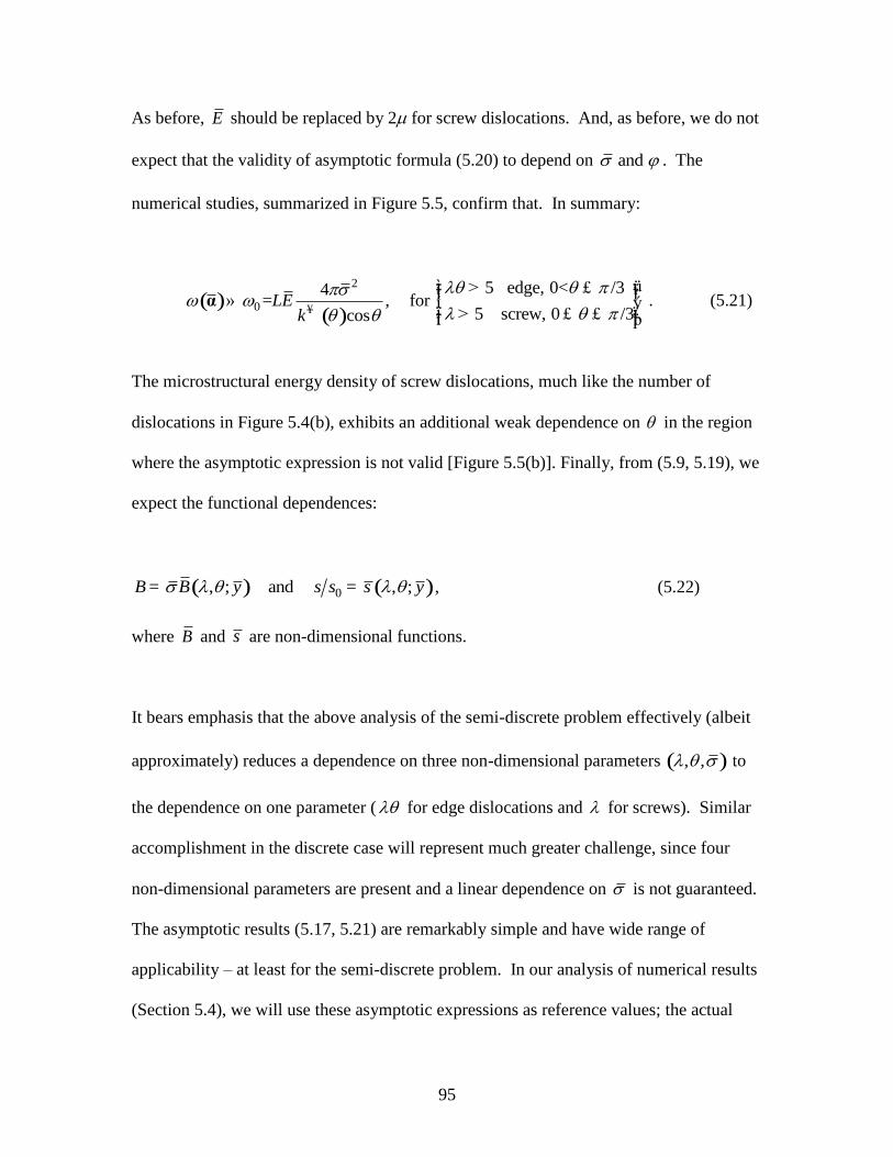
95

As before, E should be replaced by 2 for screw dislocations. And, as before, we do not

expect that the validity of asymptotic formula (5.20) to depend on and . The

numerical studies, summarized in Figure 5.5, confirm that. In summary:

( )( )

2

0

5 edge, 0< /34= , for

5 screw, 0 /3cosLE

k

¥

í ü> £ï ïï ï» ì ýï ï> £ £ï ïî þ

α . (5.21)

The microstructural energy density of screw dislocations, much like the number of

dislocations in Figure 5.4(b), exhibits an additional weak dependence on in the region

where the asymptotic expression is not valid [Figure 5.5(b)]. Finally, from (5.9, 5.19), we

expect the functional dependences:

( ) ( )0, ; and , ;B B y s s s y = = , (5.22)

where B and s are non-dimensional functions.

It bears emphasis that the above analysis of the semi-discrete problem effectively (albeit

approximately) reduces a dependence on three non-dimensional parameters ( ), , to

the dependence on one parameter ( for edge dislocations and for screws). Similar

accomplishment in the discrete case will represent much greater challenge, since four

non-dimensional parameters are present and a linear dependence on is not guaranteed.

The asymptotic results (5.17, 5.21) are remarkably simple and have wide range of

applicability – at least for the semi-discrete problem. In our analysis of numerical results

(Section 5.4), we will use these asymptotic expressions as reference values; the actual

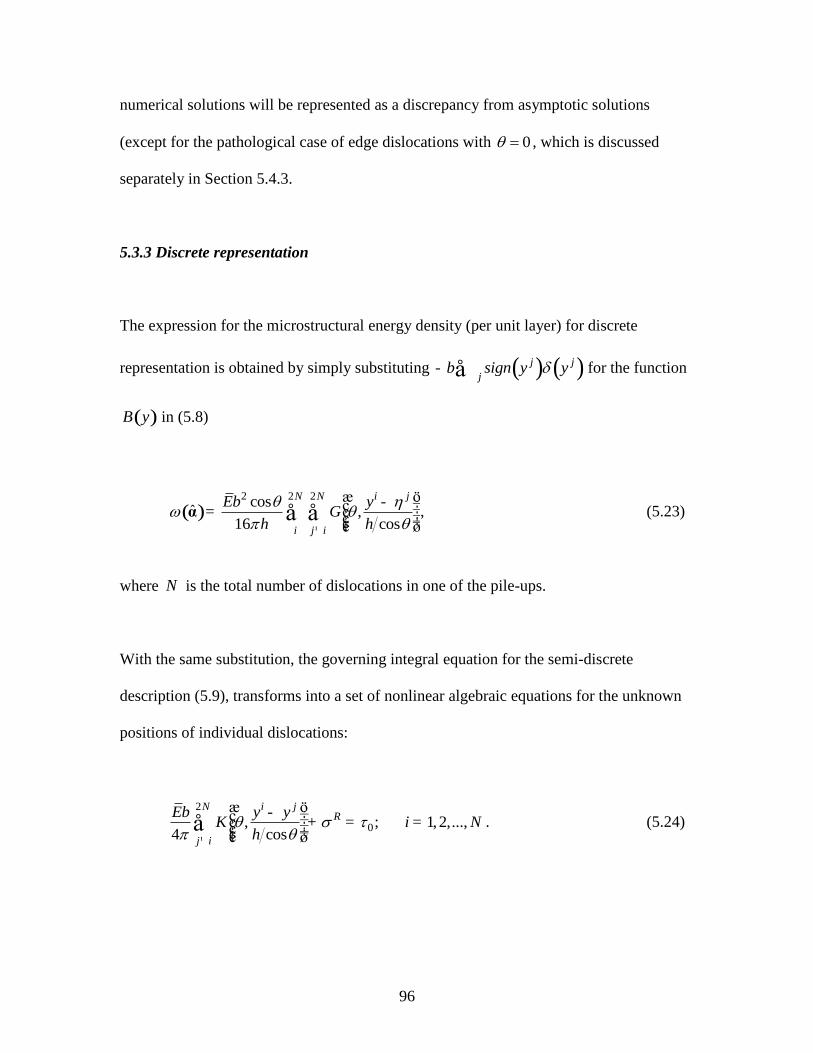
96

numerical solutions will be represented as a discrepancy from asymptotic solutions

(except for the pathological case of edge dislocations with 0 , which is discussed

separately in Section 5.4.3.

5.3.3 Discrete representation

The expression for the microstructural energy density (per unit layer) for discrete

representation is obtained by simply substituting ( ) ( )j j

jb sign y y- å for the function

( )B y in (5.8)

( )2 2 2cos

ˆ ,16 cos

i jN N

i j i

Eb yG

h h

¹

æ ö- ÷ç ÷= ç ÷ç ÷÷çè øå åα , (5.23)

where N is the total number of dislocations in one of the pile-ups.

With the same substitution, the governing integral equation for the semi-discrete

description (5.9), transforms into a set of nonlinear algebraic equations for the unknown

positions of individual dislocations:

2

0, ; 1,2,...,4 cos

i jNR

j i

Eb y yK i N

h

¹

æ ö- ÷ç ÷+ = =ç ÷ç ÷÷çè øå . (5.24)

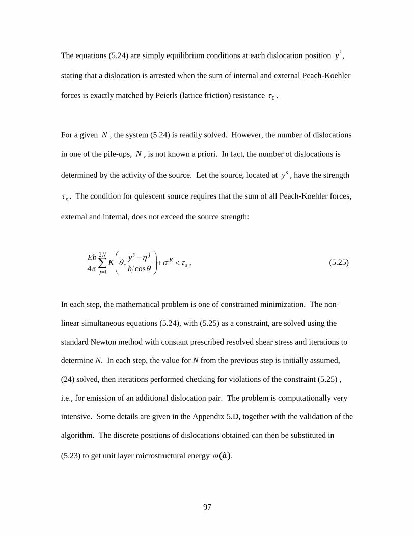
97

The equations (5.24) are simply equilibrium conditions at each dislocation position iy ,

stating that a dislocation is arrested when the sum of internal and external Peach-Koehler

forces is exactly matched by Peierls (lattice friction) resistance 0 .

For a given N , the system (5.24) is readily solved. However, the number of dislocations

in one of the pile-ups, N , is not known a priori. In fact, the number of dislocations is

determined by the activity of the source. Let the source, located at sy , have the strength

s . The condition for quiescent source requires that the sum of all Peach-Koehler forces,

external and internal, does not exceed the source strength:

2

1

,4 cos

s jNR

s

j

Eb yK

h

, (5.25)

In each step, the mathematical problem is one of constrained minimization. The non-

linear simultaneous equations (5.24), with (5.25) as a constraint, are solved using the

standard Newton method with constant prescribed resolved shear stress and iterations to

determine N. In each step, the value for N from the previous step is initially assumed,

(24) solved, then iterations performed checking for violations of the constraint (5.25) ,

i.e., for emission of an additional dislocation pair. The problem is computationally very

intensive. Some details are given in the Appendix 5.D, together with the validation of the

algorithm. The discrete positions of dislocations obtained can then be substituted in

(5.23) to get unit layer microstructural energy ( )ˆ α .

98

Problems formulated using the discrete description have three characteristic lengths: the

Burgers vector b, the slip plane spacing h, and, the half-width of the film, L. Thus, two

non-dimensional length ratios will appear as independent variables: (5.12), and

(5.15). For the discrete representation, one can formally define the slip discontinuity s ,

consisting of steps at each dislocation position. Similarly, the dislocation density

distribution B can take a form of steps, if each dislocation is smeared within the two half-

intervals between itself and its nearest neighbors. These functions, as well as the number

of dislocations N, will now not only depend on the parameter , but may be have

nonlinear dependence on . The functional dependence on the microstructural energy

density (5.23) is consequently more complex than in the semi-discrete case.

Finally, all functions of interest will, in general, depend on the Peierls lattice friction 0

(5.9, 5.24), and on the source strength s (5.25). For most metals, the applied stresses of

interest are much higher than either 0 or s , particularly if dislocation pile-ups with the

resulting back-stresses are involved. For example, for fcc metals, 0 and s are of the

order of 1 MPa ( 510 : ), while the applied stresses of interest are of the order 100 MPa

( 310 : ). In our study, we set 0 0s .

5.4 Numerical results and analysis

99

Pile-ups of edge and screw dislocations, in periodically spaced slip planes, inclined at

angle to the 1x -axis (Figure 5.2), are analyzed numerically. The case of edge

dislocations piling-up in slip planes orthogonal to the boundary ( )0 = is qualitatively

different from other cases, since it produces no long-range stresses. It is discussed

separately is Section 5.4.3.

In general, the solutions to the semi-discrete problem are expected to depend on four non-

dimensional parameters ( ), , , . Our goal is to define the limits of validity of

asymptotic expressions (5.17, 5.20) in terms of as few parameters as possible. To that

end, we have conducted a comprehensive numerical study using both, the semi-discrete

and the discrete descriptions. The results are summarized below.

5.4.1 Number of dislocations in a pile-up and the microstructural energy

In Section 5.3.2, we have established conditions for validity of asymptotic expression for

number of dislocations N , obtained from the semi-discrete representation (5.17). Now,

we consider discrete representation. In our numerical studies, we have found that the

limits of validity of asymptotic expressions (5.17, 5.20) are much more complex for edge

dislocations then for screws.

The results for number of dislocations are summarized in Figure 5.6, where the

asymptotic, non-integer value 0N is replaced by its larger integer approximation. To

100

arrive at dependence on the single parameter ( )

1 4

for edge dislocations, we have

first confirmed that the dependence can be reduced to two parameters: – a guess

inspired by semi-discrete solutions (Figures 5.4 and 5.5), and – inspired by the form

of asymptotic solution (5.17). Then, we plotted the transition points between numerical

solutions for which the asymptotic (5.17) is valid within 5% error and those for which the

asymptotic is not valid in ( )ln , ln

plane to obtain a straight line with slope ¼. In

summary:

[ ]( )

1 4

0 0

1, edged.ˆ int +1, for 1, screw d.

N N N

í üï ï>ï ï» = ì ýï ï>ï ïî þ

. (5.26)

The number of dislocations N, in a pile-up on one side, is found while solving equation

(5.24) for equilibrium positions of dislocations. Since for edge dislocations

20 sin 2N -µ (5.11, 5.14), the number of edge dislocations in the pile-up will have a

minimum at 4 = . However, for screw dislocations, 20 cosN -µ , so that the

number of dislocations in the pile-up steadily increases with increasing θ.

We now consider microstructural energy density obtained from discrete representation

(5.23), ( )ˆ ˆ ºα . The discrete microstructural energy density is expected to require

more complicated conditions for validating asymptotic approximation than those

described in section 5.3.2 (Figure 5.5) for the semi-discrete microstructural energy

density. In particular, we expect that the number of dislocations must be high enough if

101

the asymptotic expression (5.20) is to hold. This is indeed true, as shown in Figure 5.7.

From Figures 5.7 and 5.8:

( )

1 4

00 0

0

ˆ5 and 10, edge d.ˆˆ ˆ = , for

ˆ5 and 10, screw d.

NLE N

N

í üï ï> >ï ïï ï» ì ýï ï> >ï ïï ïî þ

. (5.27)

In Figure 5.7, large scatter of data is noticeable for screw dislocations for 0ˆ 20N < . With

increasing 0N , this scatter disappears. In Figure 5.8(b), the weak dependence of

microstructural energy on and ( ) is apparent, even for 1 > . Moreover, the

discrete microstructural energy seems to converge to values theta are up to 5% different

from 0 . We consider these variations too small to justify the additional complications

required to resolve them.

5.4.2 Slip distributions

Based on (5.19, 5.17), we expect that the discrete slip distribution is close to the semi-

discrete one if 1 (edge) , and 1 (screw) . That, however, is not sufficient. Our

numerical analysis, illustrated in Figure 5.9, suggests that the number of dislocations

must be high enough, roughly 10N , if the two slip distribution are to be similar.

As discussed earlier, the solutions are characterized by highly localized dislocation

distributions near the boundary, as shown in Figures 5.9 and 5.10, which produce a

102

uniform back stress, except in a small region near the boundary. The localization

intensifies with increasing , as evident in Figure 5.9. The dependence on the slip plane

inclination, θ, is shown in Figure 5.10. For screw dislocations, boundary localization

intensifies with decreasing θ. For edge dislocations, localization intensifies with

increasing θ, up to 4 = , where it begins to relax as θ increases further. In this, the

localization follows the number of dislocations, which is discussed in the previous

section; the fewer dislocations, the more intense the localization.

5.4.3 Special case: edge dislocations in slip planes orthogonal to the boundary

In this case, the long-range stresses are non-existent, i.e. the stresses vanish outside the

interval h (Figure 5.3). Consequently, the number of dislocations in pile-up increases

rapidly with increasing stress. The asymptotic expressions for number of dislocations

(5.14), and energy density (5.20) are not applicable for this case, since ( )0 0k¥ = for

edge dislocations (5.11). Instead, we obtain an accurate asymptotic curve fit (large ) to

semi-discrete computational results, for: the number of dislocations N (5.13) and the

energy density ( ) ºα (5.8). From Figure 5.11:

( )

( )

0

20

4 1.5 0.567 , for 1,

81.53 0.986 , for 5.

N N

EL

^

^

» = + >

» = + > (5.28)

0

s

s

103

However, for discrete problem, this is not the sufficient condition. The approximation

fails for small values of ( ) . As shown in Figure 5.12, a more complete condition can

be written as

[ ]0 0

0

ˆ int 1, for 1 and 1,

ˆ , for 5 and 1.

N N N

^ ^

^

» = + > >

» > > (5.29)

The critical value in (5.28, 5.29) is based on a relative error of less then 5% . The

conditions (5.29) are easily interpreted by means of the asymptotic expression for the

number of dislocations (5.28). Simply, the estimate (5.28) for the number of dislocations

is good if there are at least 6 dislocations in the pile-up. The energy estimate (5.28), on

the other hand, requires at least 30 dislocations in the pile-up.

Slip distributions are shown in Figure 5.13. Owing to the vanishing long-range stresses,

the number of dislocations is much larger than in the previous cases, and dislocations are

spread throughout the slip plane. The slip distribution is, roughly, a parabola, except at

the boundaries where there is a small singular portion. Slip distributions computed from

discrete representation are close to those obtained for semi-discrete representation even

for small values of .

5.5 Summary

104

Pile-ups of dislocations, stacked in equidistant slip planes, in plane strain (edge) and anti-

plane (screw) conditions, are studied using two different representations of dislocations:

discrete and semi-discrete. The configuration consists of a thin elastic plastic film,

embedded into elastic medium.

Dimensional analysis yielded one non-dimensional stress parameter (5.16) and two non-

dimensional length parameters: the ratio of the film thickness and the slip plane spacing

(5.12) and the ratio of the slip plane spacing and the Burgers vector (5.15).

Asymptotic expressions for number of dislocations, maximum slip, and microstructural

energy density are derived for the general case:

0 0 0 0 0 0

4 ˆ ˆ, int +1, or cos

N N N LE N Nk

. (5.30)

The special case of edge dislocations piling-up in slip planes orthogonal to the boundary

is qualitatively different from other cases as it produces zero long-range stresses.

Asymptotic expressions for this case have been developed numerically (5.28, 5.29).

Based on the comprehensive numerical study of the parameter space, the conditions for

validity of asymptotic expressions are found. These are summarized in Table 5.1.

Owing to the long-range stresses, the distributions are highly localized near the boundary;

the localization intensifies with for both edge and screw dislocations. For screw

dislocations, boundary localization decreases with θ; while for edge dislocations,

105

localization intensifies with increasing θ, up to 4 = , where it begins to relax as θ

increases further. In the special case of edge pile-ups with 0 = dislocations pile-up in

large numbers and are spread throughout the slip plane producing a parabolic slip

distribution with a small singular portion at the boundaries.

Acknowledgements

This work was supported by the US National Science Foundation, grant # CMS-0528550,

and, the US Department of Energy, grant # DE-FG02-05ER25709.

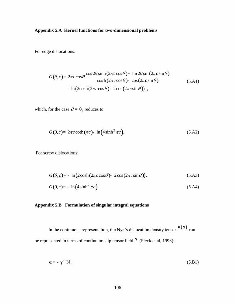
106

Appendix 5.A Kernel functions for two-dimensional problems

For edge dislocations:

( )

( ) ( )

( ) ( )

( ) ( )( )

cos 2 sinh 2 cos sin 2 sin 2 sin, 2 cos

cos h 2 cos cos 2 sin

ln 2cosh 2 cos 2cos 2 sin ,

c cG c c

c c

c c

+=

-

- -

(5.A1)

which, for the case 0 = , reduces to

( ) ( ) ( )20, 2 coth ln 4sinhG c c c c = - . (5.A2)

For screw dislocations:

( ) ( ) ( )( ), ln 2cosh 2 cos 2cos 2 sinG c c c = - - , (5.A3)

( ) ( )20, ln 4sinhG c c= - . (5.A4)

Appendix 5.B Formulation of singular integral equations

In the continuous representation, the Nye‟s dislocation density tensor α x

can

be represented in terms of continuum slip tensor field γ (Fleck et al, 1993):

= - ´ Ñα γ . (5.B1)

107

The slip tensor is obtained from slips on all active slip systems:

= åγ s m , (5.B2)

where unit vectors

s and

m represent the slip direction and the slip plane normal for

the slip system .

To apply the principle of virtual work to the problem at hand, we first note that a version

of microstructural energy (5.5), computed from the continuous representation (5.4), is

included in the standard elastic strain energy. Separation of the microstructural energy

from the elastic strain energy requires separation of compatible and incompatible elastic

strains. The details of the general procedure are given in the forthcoming paper

(Mesarovic et.al, 2009). When the configuration in Figure 5.2 is loaded only by the far-

field stress 12, the compatible elastic strain is the average elastic shear

( )2 22 1

12 21 11 2

1sin cos

2 2

L

L

u s u se e dx

L x h x h

-

í üï ï¶ ¶ï ï= = + + -ì ýï ï¶ ¶ï ïî þ

ò , (5.B3)

where s is the displacement discontinuity across the slip plane, and iu are components of

a continuous, single-valued displacement field. The principle of virtual work (per unit

layer) is then written as

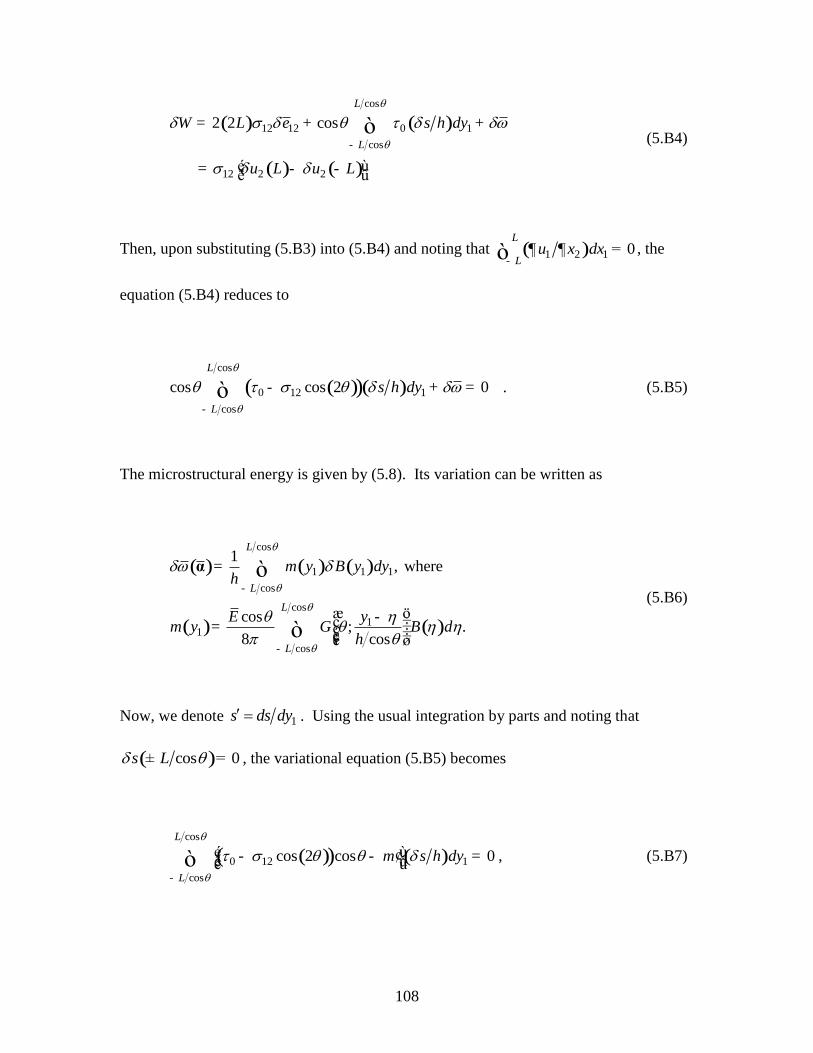
108

( ) ( )

( ) ( )

cos

12 12 0 1

cos

12 2 2

2 2 cos

L

L

W L e s h dy

u L u L

-

= + +

é ù= - -ë û

ò (5.B4)

Then, upon substituting (5.B3) into (5.B4) and noting that ( )1 2 1 0L

Lu x dx

-¶ ¶ =ò , the

equation (5.B4) reduces to

( )( )( )

cos

0 12 1

cos

cos cos 2 0

L

L

s h dy

-

- + =ò . (5.B5)

The microstructural energy is given by (5.8). Its variation can be written as

( ) ( ) ( )

( ) ( )

cos

1 1 1

cos

cos

11

cos

1, where

cos; .

8 cos

L

L

L

L

m y B y dyh

E ym y G B d

h

α

-

-

=

æ ö- ÷ç ÷= ç ÷ç ÷çè ø

ò

ò

(5.B6)

Now, we denote 1s ds dy . Using the usual integration by parts and noting that

( )cos 0s L ± = , the variational equation (5.B5) becomes

( )( ) ( )

cos

0 12 1

cos

cos 2 cos 0

L

L

m s h dy

-

é ù¢- - =ê úë ûò , (5.B7)

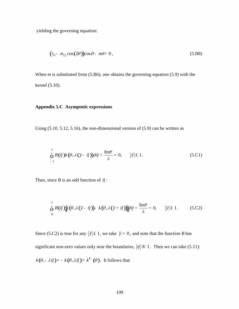
109

yielding the governing equation:

( )( )0 12 cos 2 cos 0m ¢- - = , (5.B8)

When m is substituted from (5.B6), one obtains the governing equation (5.9) with the

kernel (5.10).

Appendix 5.C Asymptotic expressions

Using (5.10, 5.12, 5.16), the non-dimensional version of (5.9) can be written as

( ) ( )( )1

1

8, 0, 1B k y d y

-

- + = £ò . (5.C1)

Then, since B is an odd function of

( ) ( )( ) ( )( )1

0

8, , 0, 1B k y k y d y

é ù- - + + = £ê úë ûò . (5.C2)

Since (5.C2) is true for any 1y £ , we take 0y = , and note that the function B has

significant non-zero values only near the boundaries, 1 ® . Then we can take (5.11):

( ) ( ) ( ), ,k k k ¥- = - = . It follows that

110

( )( )

1

0

4B d

k

¥- =ò . (5.C3)

Upon substitution of (5.C3) into (5.13), the asymptotic expression (5.14) is derived.

To derive the asymptotic expression for energy density (5.8), we first note that, using

(5.10), the integral in (5.9) is the derivative of inner integral in (5.8) with respect to y.

Thus, the energy expression (5.8) can be written as

( ) ( )( ) ( )

cos 1

cos 1

cos8

16 2 cos

L

L

EdyB y y EL yB y dy

h

α

- -

= - = -ò ò . (5.C4)

Since B is concentrated near the boundary, the approximation for the integral is obtained

by taking 1y = ± , whereupon the expression (5.C3) can be used:

( ) ( )( )

1 1

1 0

82yB y dy B d

k

¥

-

- » - =ò ò , (5.C5)

which yields the asymptotic expression (5.20).

Appendix 5.D Numerical methods

Semi-discrete representation. The numerical method for solving (5.9) was developed by

Erdogan & Gupta (1972). The singularities of ( )B at 1 = ± are of the order

2 1 2(1 ) , so that:

111

( ) ( ) 21B = - . (5.D1)

The unknown regular function ( ) is approximated using the Chebyshev polynomials

of the first kind, ( )mT :

( ) ( )0

n

m m

m

b T =

= å . (5.D2)

When (5.D1) and (5.D2) are substituted into (5.9), the properties of Chebyshev

polynomials dictate the necessary condition for (5.9) in a form of the system of n linear

algebraic equations for n unknowns ( ), 1,...,k k n = , where k are the zero‟s of

Chebyshev polynomials. The solution provides the function ( ) , and thus ( )B

(5.D1).

Discrete representation. The equilibrium positions of dislocations in the pile-up are

computed by solving non-linear equations (5.24), under the constraint (5.25). Let the

first N pairs of dislocations in a double ended pile-up be equilibrated, and the next,

(N+1)th

pair has nucleated. Its equilibrium position is calculated iteratively. In the first

iteration, the crude approximation for the position of the new pair is obtained by keeping

the original N pairs locked in their previous positions, and solving (5.24). This is then the

starting point for Newton-Raphson iterations until the equilibrium positions of all pairs

are found.

112

The procedure is computationally intensive. The long-range interactions imply the full

system matrix. Moreover, the change of positions in each step require full matrix

inversion in each step, so that the number of operation for Nth

step is of the order 3N .

Therefore, the total number of operations scales with 4N . To validate the algorithm and

the numerical code, we considered the single-ended pile-up on a single slip plane, and

compared our numerical result to the Eshelby et al (1951) analytical solutions. Apart

from a negligible round-off error, the agreement between two sets of dislocation positions

was perfect.

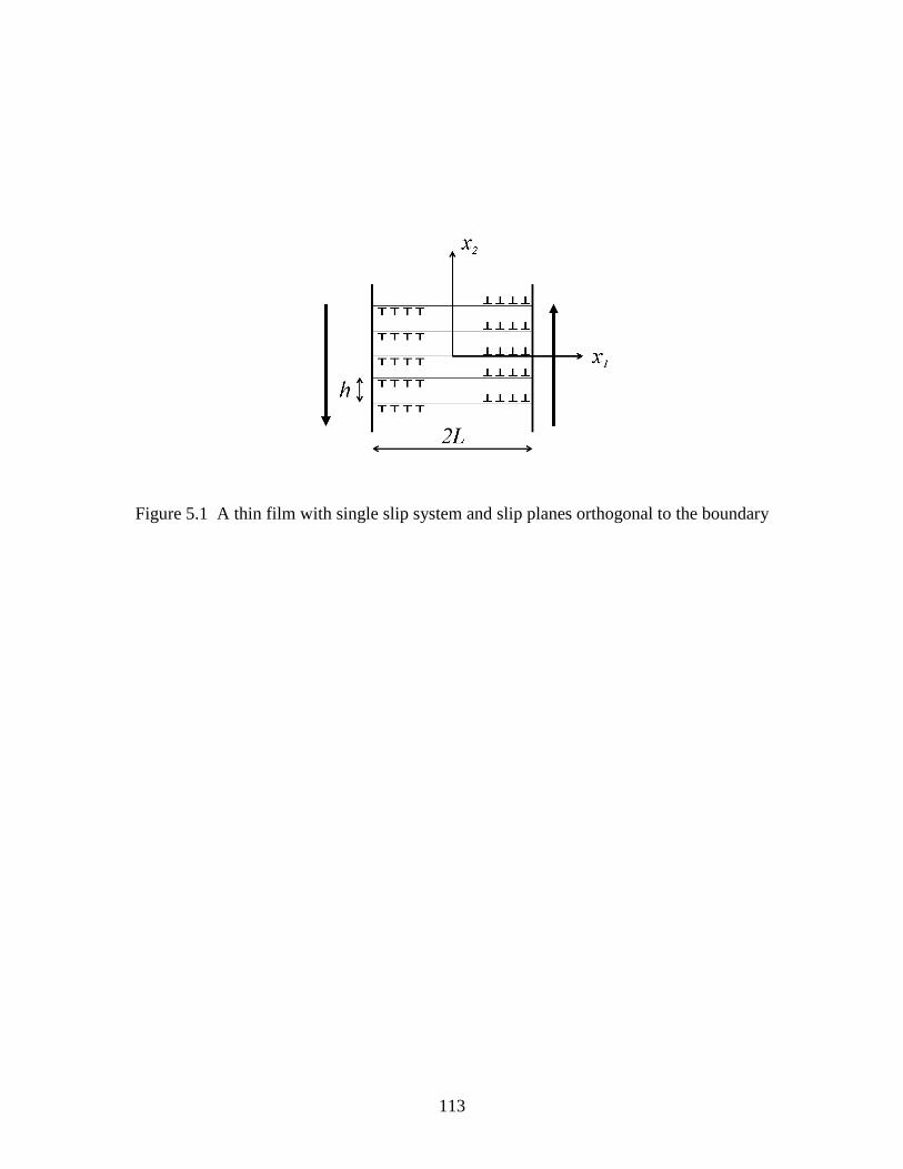
113

Figure 5.1 A thin film with single slip system and slip planes orthogonal to the boundary

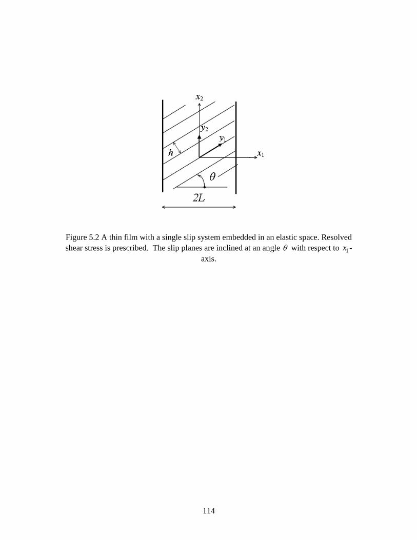
114

Figure 5.2 A thin film with a single slip system embedded in an elastic space. Resolved

shear stress is prescribed. The slip planes are inclined at an angle with respect to 1x -

axis.

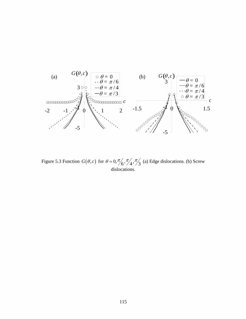
115

Figure 5.3 Function ,G c for 0, , ,6 4 3

(a) Edge dislocations. (b) Screw

dislocations.

-5

-1

3

-2 -1 0 1 2

θ=0θ=π/6θ=π/4θ=π/3

0 =/ 6 =/ 4 =/ 3 =

( ),G c

c

(a)

-5

-1

3

-1.5 0 1.5

θ=0θ=π/6θ=π/4θ=π/3

0 =/ 6 =/ 4 =/ 3 =

( ),G c

c

(b)

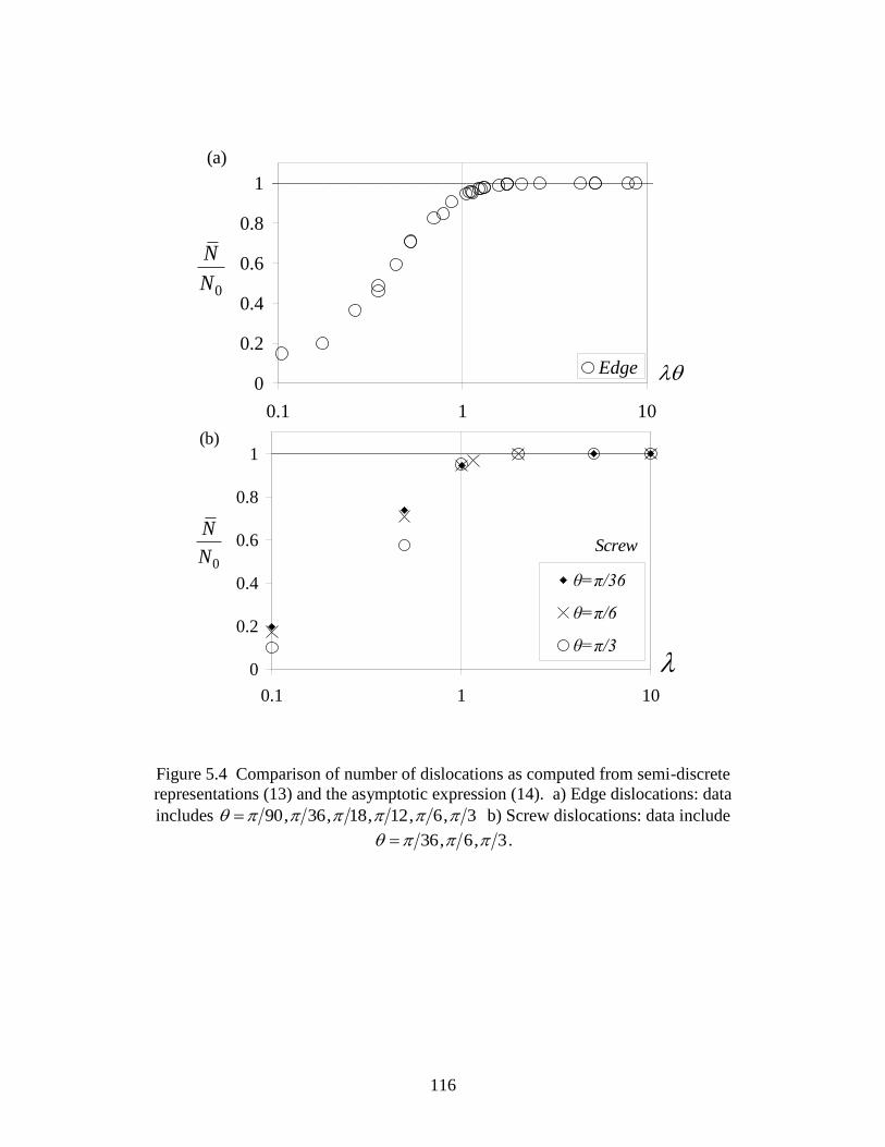
116

Figure 5.4 Comparison of number of dislocations as computed from semi-discrete

representations (13) and the asymptotic expression (14). a) Edge dislocations: data

includes 90, 36, 18, 12, 6, 3 b) Screw dislocations: data include

36, 6, 3 .

0

0.2

0.4

0.6

0.8

1

0.1 1 10

Edge

0

N

N

(a)

(b)

0

0.2

0.4

0.6

0.8

1

0.1 1 10

θ=π/36

θ=π/6

θ=π/3

0

N

N

Screw

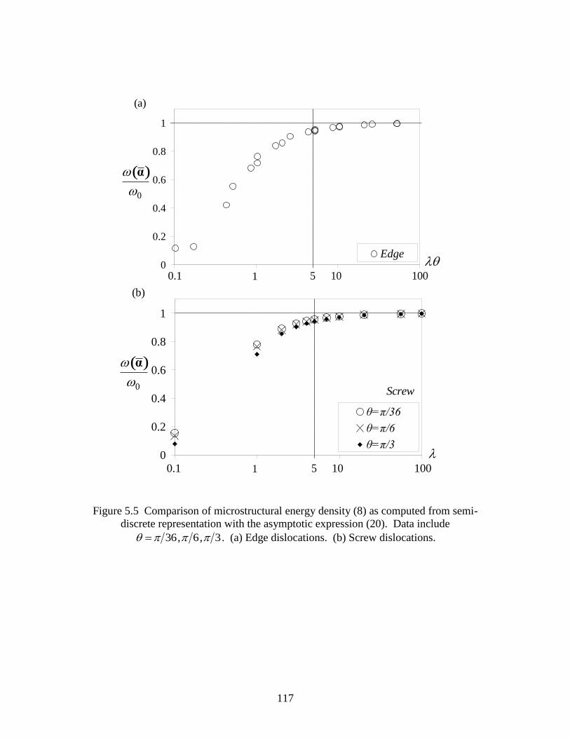
117

Figure 5.5 Comparison of microstructural energy density (8) as computed from semi-

discrete representation with the asymptotic expression (20). Data include

36, 6, 3 . (a) Edge dislocations. (b) Screw dislocations.

0

0.2

0.4

0.6

0.8

1

0.1 1 10 100

Edge

( )

0

α

(a)

0.1 1 5 10 100

0

0.2

0.4

0.6

0.8

1

0.1 1 10 100

θ=π/36

θ=π/6

θ=π/3

( )

0

α

(b)

0.1 1 5 10 100

Screw

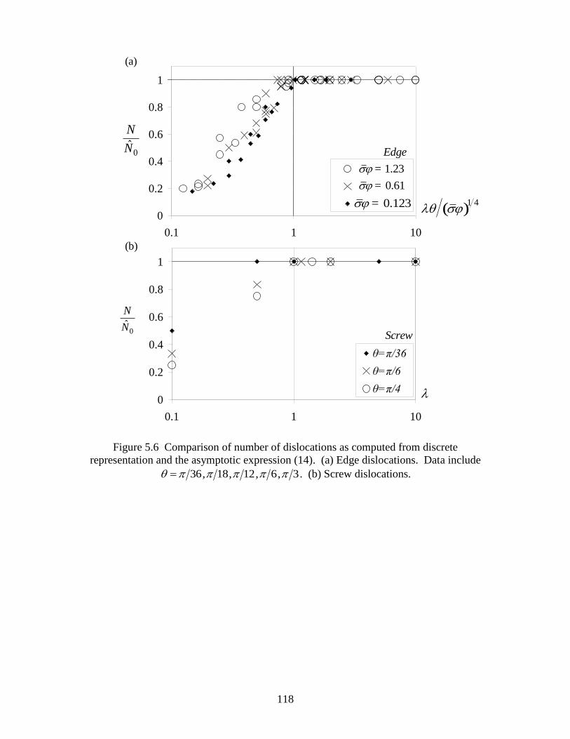
118

Figure 5.6 Comparison of number of dislocations as computed from discrete

representation and the asymptotic expression (14). (a) Edge dislocations. Data include

36, 18, 12, 6, 3 . (b) Screw dislocations.

0

0.2

0.4

0.6

0.8

1

0.1 1 10

σφ=1.23

σφ=0.61

σφ=0.123

0ˆ

N

N

( )1 4

1.23 =

0.61 =

0.123 =

Edge

(a)

0

0.2

0.4

0.6

0.8

1

0.1 1 10

θ=π/36

θ=π/6

θ=π/4

0ˆ

N

N

Screw

(b)

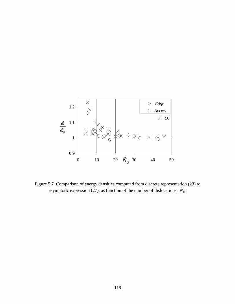
119

Figure 5.7 Comparison of energy densities computed from discrete representation (23) to

asymptotic expression (27), as function of the number of dislocations, 0N .

0.9

1

1.1

1.2

0 10 20 30 40 50

Edge

Screw

0N

0

ˆ

ˆ

Edge

Screw

50

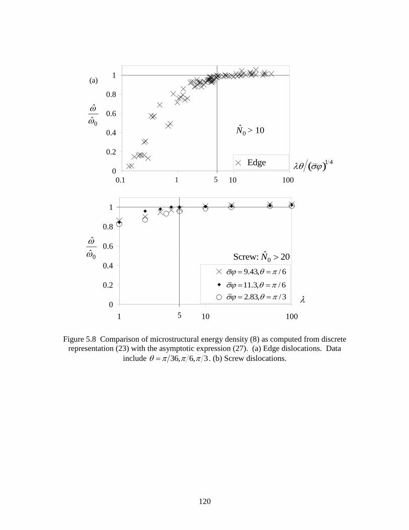
120

Figure 5.8 Comparison of microstructural energy density (8) as computed from discrete

representation (23) with the asymptotic expression (27). (a) Edge dislocations. Data

include 36, 6, 3 . (b) Screw dislocations.

0

0.2

0.4

0.6

0.8

1

0.1 1 10 100

Edge - N>10

(a)

0.1 10 100

0

ˆ

ˆ

( )1 4

1 5

Edge

0ˆ 10N >

0

0.2

0.4

0.6

0.8

1

1 10 100

σφ=9.43,θ=π/6

Series1

σφ=2.83,θ=π/3

9.43, / 6

11.3, / 6

2.83, /3

0ˆScrew: 20N

0

ˆ

ˆ

5

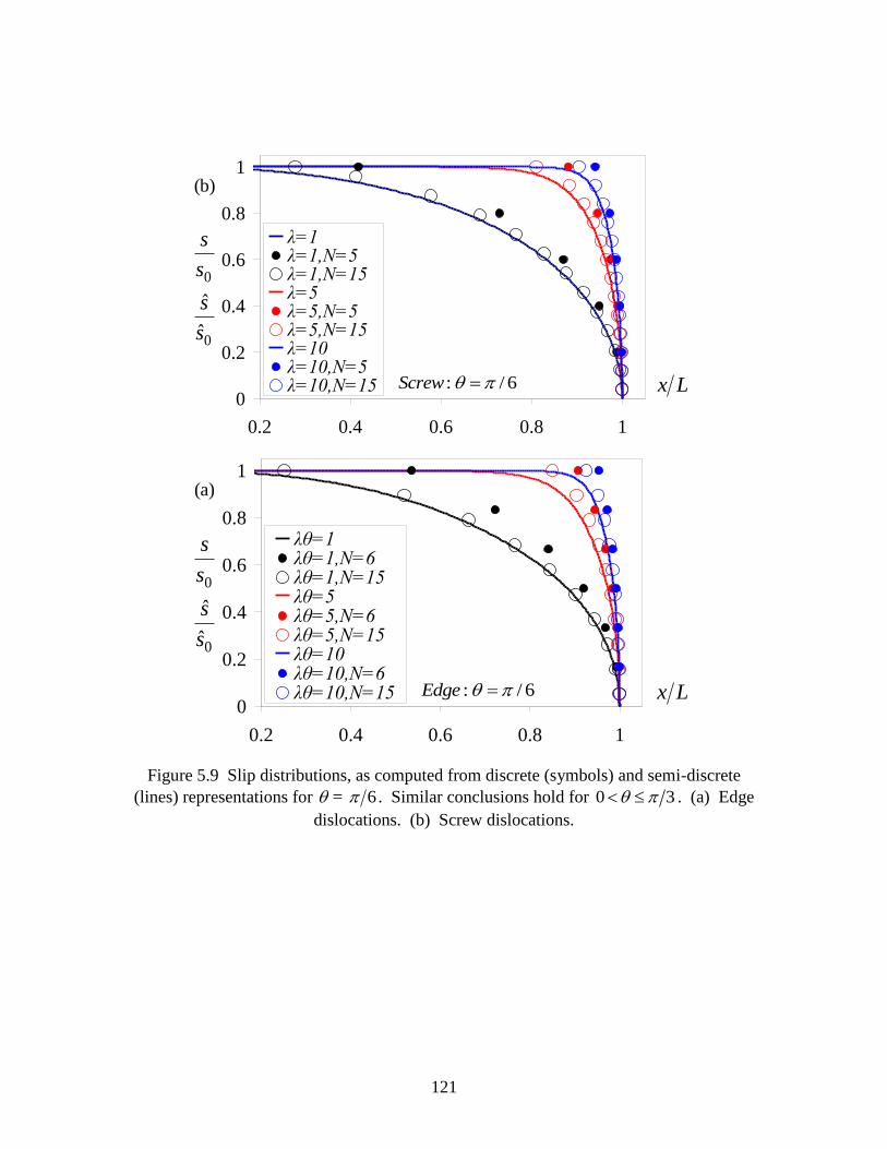
121

Figure 5.9 Slip distributions, as computed from discrete (symbols) and semi-discrete

(lines) representations for 6 = . Similar conclusions hold for 0 3 . (a) Edge

dislocations. (b) Screw dislocations.

0

0.2

0.4

0.6

0.8

1

0.2 0.4 0.6 0.8 1

λ=1λ=1,N=5λ=1,N=15λ=5λ=5,N=5λ=5,N=15λ=10λ=10,N=5λ=10,N=15

0

0

ˆ

ˆ

s

s

s

s

x L: / 6Screw

(b)

0

0.2

0.4

0.6

0.8

1

0.2 0.4 0.6 0.8 1

λθ=1λθ=1,N=6λθ=1,N=15λθ=5λθ=5,N=6λθ=5,N=15λθ=10λθ=10,N=6λθ=10,N=15

0

0

ˆ

ˆ

s

s

s

s

x L: / 6Edge

(a)

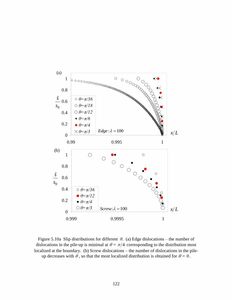
122

Figure 5.10a Slip distributions for different θ. (a) Edge dislocations – the number of

dislocations in the pile-up is minimal at 4 = corresponding to the distribution most

localized at the boundary. (b) Screw dislocations – the number of dislocations in the pile-

up decreases with , so that the most localized distribution is obtained for 0 = .

0

0.2

0.4

0.6

0.8

1

0.99 0.995 1

θ=π/36

θ=π/18

θ=π/12

θ=π/6

θ=π/4

θ=π/3

(a)

0

s

s

x L: 100Edge

0

0.2

0.4

0.6

0.8

1

0.999 0.9995 1

θ=π/36

θ=π/12

θ=π/4

θ=π/3

(b)

0

s

s

x L: 100Screw

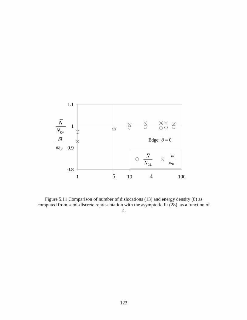
123

Figure 5.11 Comparison of number of dislocations (13) and energy density (8) as

computed from semi-discrete representation with the asymptotic fit (28), as a function of

.

0.8

0.9

1

1.1

1 10 100

NSD WSD

5

0

N

N 0

Edge: 0

0

0

N

N

^

^

124

Figure 5.12 Comparison of number of dislocations and energy density (23) as computed

from discrete representation with the asymptotic fit (29), as a function of . The

scatter of data indicates different values of .

0

1

2

3

4

0 1 2 3 4

ND wD0

ˆ

N

N 0

ˆ

ˆ

0

0

ˆ

ˆ

N

N

^

^

: 0, 5Edge

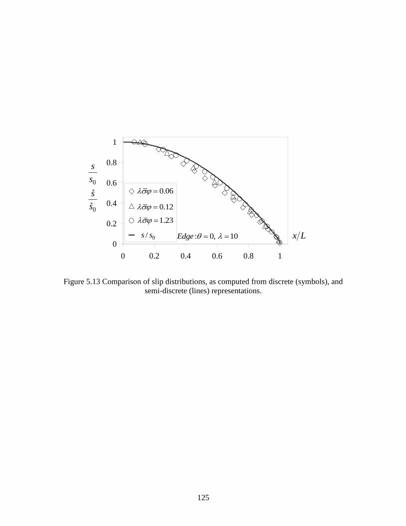
125

Figure 5.13 Comparison of slip distributions, as computed from discrete (symbols), and

semi-discrete (lines) representations.

0

0.2

0.4

0.6

0.8

1

0 0.2 0.4 0.6 0.8 1

λσφ=0.06

λσφ=0.123

λσφ=1.23

φ=∞

0

0

ˆ

ˆ

s

s

s

s

0.06

x L: 0, 10Edge

0.12

1.23

0/s s

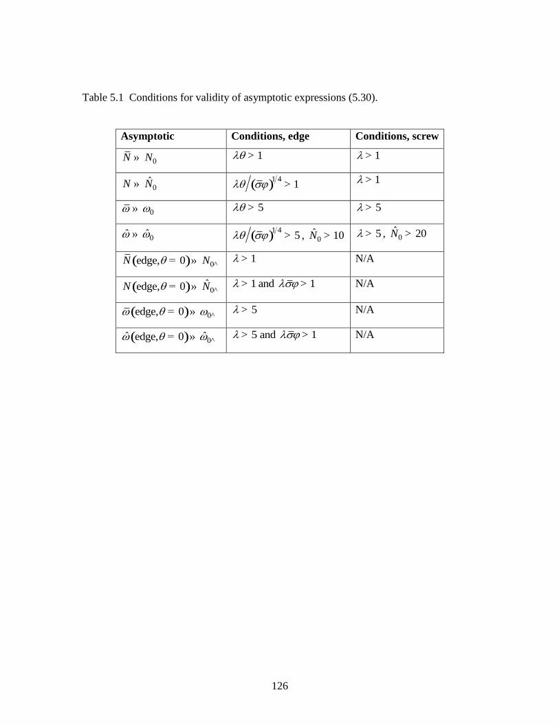
126

Table 5.1 Conditions for validity of asymptotic expressions (5.30).

Asymptotic Conditions, edge Conditions, screw

0N N» 1 > 1 >

0ˆN N» ( )

1 41 > 1 >

0 » 5 > 5 >

0ˆ ˆ » ( )

1 45 > , 0

ˆ 10N > 5 > , 0ˆ 20N >

( ) 0edge, 0N N ^= » 1 > N/A

( ) 0ˆedge, 0N N ^= » 1 and 1 > > N/A

( ) 0edge, 0 ^= » 5 > N/A

( ) 0ˆ ˆedge, 0 ^= » 5 and 1 > > N/A

127

CHAPTER SIX: SUMMARY AND FUTURE WORK

In this work, we have developed an approach to deal with short and long range

interactions of dislocations. For the homogeneous anisotropic medium, the short range

interactions are dealt with by combining the Mura‟s line integral with anisotropic Greens

tensor derivatives. An algorithm was developed to numerically integrate the Greens

tensor derivatives in conjunction with the numerical integration of Mura‟s integral for the

stress field due to a dislocation segment. For the case of inhomogeneous media, we have

developed a new approach and derived analytical expressions for the stress field due to a

dislocation segment in an isotropic bi-material medium. The derived expressions are

validated with the results existing in the literature and special cases such as dislocation

segment near a traction-free surface, rigid surface and in the interface are degenerated.

The line integrals for the stress field due to discrete dislocation segment in homogeneous

and inhomogeneous media are naturally extended to volume integrals for the stress field

due to continuously distributed distributions to deal with long-range interactions of

dislocations.

As a future work, our study on line integral for image stresses due to dislocation segment

in 3D bi-material medium can be incorporated in the dislocation dynamics codes to

investigate the interactions of dislocations in multi-layered metallic composites. In

chapter four, we have investigated interaction of dislocations with pure tilt wall. After the

transmission of several dislocations through the pure tilt, the boundary with a large offset

relaxes to a configuration consisting of an array of disclination dipoles with a grain

boundary dislocation. As a future work, molecular dynamics simulations of interactions

128

of several dislocations with pure tilt wall can be done to thoroughly understand the path

and process of relaxation.

As a digression from the main theme, in chapter five, we have studied the kinematic and

thermodynamic effects due to different representation of discrete dislocations. The error

in number of dislocations, microstructural energy and slip distributions due to semi-

discrete dislocations is quantified. A dimensional analysis is done and the threshold

values for certain key parameters are deduced from asymptotic expressions. This work is

used in the development of a size dependent crystal plasticity theory.

In appendix, we investigated the macroscopic deformation and microscopic dislocation

mechanisms of micropillars under uniaxial compression experiment using multi-scale

discrete dislocation plasticity approach. We have discovered the key dislocation

mechanism responsible for the observed slip bursts and strain hardening. We mainly

concluded the observed plastic deformation is due dislocation stagnation caused by the

formation of entangled dislocation structures and reduction in the mean free length of the

dislocation arms.

129

International Journal of Plasticity (accepted)

APPENDIX A: ANALYSIS OF HETEROGENEOUS DEFORMATION AND

DISLOCATION DYNAMICS IN SINGLE CRYSTAL MICROPILLARS UNDER

COMPRESSION

S Akarapu, H M Zbib, and DF Bahr

School of Mechanical and Materials Engineering

Washington State University, Pullman, WA, 99164-2920

Abstract

The size dependent deformation of Cu single crystal micropillars with thickness ranging

from 0.2 to 2.5 m subjected to uniaxial compression is investigated using a Multi-scale

Discrete Dislocation Plasticity (MDDP) approach. MDDP is a hybrid elasto-visco plastic

simulation model which couples discrete dislocation dynamics at the micro-scale

(software micro3d) with the macroscopic plastic deformation. Our results show that the

deformation field in these micropillars is heterogeneous from the onset of plastic flow

and is confined to few deformation bands, leading to the formation of ledges and stress

concentrations at the surface of the specimen. Furthermore, the simulation yields a

serrated stress-strain behavior consisting of discrete strain bursts that correlates well with

experimental observations. The intermittent operation and stagnation of discrete

dislocation arms is identified as the prominent mechanism that causes heterogeneous

deformation and results in the observed macroscopic strain bursts. We show that the

critical stress to bow an average maximum dislocation arm, whose length changes during

deformation due to pinning events, is responsible for the observed size dependent

response of the single crystals. We also reveal that hardening rates, similar to that shown

experimentally, occur under relatively constant dislocation densities and are linked to

130

dislocation stagnation due to the formation of entangled dislocation configuration and

pinning sites.

Key words: Size effect, micropillars, dislocation dynamics, micro3d

131

A.1 Introduction

Current trends in the miniaturization of micro-electronic-mechanical systems, medical

devices, and microelectronic devices have lead to systems that consist of multiscale

structural components whose dimensions, or the dimensions of their substructure, lie in

the range of a few nanometers to a few micrometers, with extremely large surface-to-

volume ratios, ranging from 106 to 10

9 m

2/m

3. At these length scales the mechanical

properties can vary significantly with decreasing dimensions. Many experiments by

several groups have shown that in metallic systems as the dimensions are reduced to

below a few micrometers the material begins to exhibit extremely high strengths, within a

fraction of the theoretical strength. This behavior is not only confined to a component

made of single material, such as in thin membranes, nanobeams, nanotubes, microbeams

and micropillars [ see e.g. (Fleck et al. 1994), (Stolken and Evans 1998), (Dimiduk et al.

2005), (Greer and Nix 2005), (Volkert and Lilleodden 2006), (Frick et al. 2008)], but is

also observed in nanolaminate metallic systems [see e.g. (Koehler 1970), (Oberle and

Cammarata 1995), (Was and Foecke 1996), (Misra et al. 1998), (Clemens et al. 1999),

(Misra and Kung 2001), (Misra et al. 2003)] which, in addition to high strength, exhibit

very high fatigue resistance [(Stoudt et al. 2001), (Zhang et al. 2005), (Wang et al.

2006)], morphological stability even at high temperatures, (Mara et al. 2004), and

fracture resistance even after large plastic deformation, (Misra et al. 2004). However,

accurate determination of mechanical properties at these length scales remains a very

challenging problem. More so is the issue of modeling of the behavior of systems that

may contain components with sub-micrometer dimensions.

132

Although the nanoindentation technique is the most frequently used method to determine

mechanical properties, there are several problems that arise when using such a technique

at the submicron scale. Because of the complexity of the stress-strain field under the

indenter tip, extraction of mechanical properties, such as yield strength, hardness, and

elastic properties, relies on models that may include certain assumptions and

approximations with a direct dependence on the shape and size of the indenter tip, see for

example (Nix 1989), (Bahr and Gerberich 1996), (Bahr et al. 1998), (Nibur and Bahr

2003), (Nibur et al. 2007). The complexities of the indentation stress field due to the tip

shape and the subsequent problems in adapting axisymmetric and isotropic materials

assumptions to experimental systems has led many researchers to miniaturize

conventional material test techniques, such as torsion, bending and uniaxial tests. (Fleck

et al. 1994) performed torsion experiments on microscale copper wires to show size

effects, and (Stolken and Evans 1998) carried out bending tests on nickel foils and

showed strong dependence of strength on foil thickness. In both of these experiments,

the size dependence was attributed to strain gradients that result from the formation of

dislocation walls which form in order to accommodate curvature distortion of the lattice.

However, a pioneering work by (Horstemeyer et al. 2001) showed through a molecular

dynamics simulations that size dependent behavior can exist even in the absence of strain

gradients. One of their main discoveries is the presence of a strong inverse-power

relationship between the yield strength and the volume-to-surface area ratio of the

computational cell. Subsequently, a number of experiments have been performed

confirming that size dependent behavior exists in “homogenously” deformed small scale

133

specimens where strain gradients do not exist. For example, recent experiments on

compression of single crystal micropillars for example by (Dimiduk et al. 2005), (Greer

and Nix 2006), (Volkert and Lilleodden 2006) and (Frick et al. 2008) show significant

size-effects, and the argument that the size effect is inherently due to the presence of

strain gradients resultant of inhomogeneous loading does not explain the observed size

effects in these micropillars.

Compression experiments by (Dimiduk et al. 2005) were done on gold micropillars,

micromachined using focused ion beam techniques, with diameters ranging from 200 nm

to several micrometers in the <001> loading direction. Even though the orientation is

one of high symmetry, the lack of stage II hardening in the stress-strain response leads to

an explanation based on dislocation starvation hypothesis given by (Greer and Nix

2006). According to this hypothesis, as the specimen dimensions are small and

unconstrained all the mobile dislocations glide to the surface and annihilate causing a

strain burst in the macroscopic response resulting in a dislocation free crystal, whereupon

further plastic deformation requires dislocations to nucleate under very high stresses.

(Volkert and Lilleodden 2006) and (Frick et al. 2008) have performed compression

experiments on Au and Ni micropillars respectively oriented effectively for single slip

and showed significant hardening. (Frick et al. 2008) also showed TEM micrographs of

dislocation structure in the compressed micropillars, while (Shaw et al. 2008) show

evidence of dislocation free pillars in very small pillars. Tensile tests that eliminate some

stress concentrations at the base of micropillar have been used to suggest that there are

also hardening effects due to non-uniform stresses in micromachined copper samples

134

(Kiener et al. 2008). Although these experiments capture size effects at small scale, they

seem to yield drastically different results for the same material depending on the

fabrication conditions of the test specimen which may result in different initial

dislocation structure as suggested by (Maaß et al. 2006) and (Maaß et al. 2008), as well

as boundary conditions that may result in stress-concentrations.

Size effects can be addressed from a purely continuum mechanics approach by means of

strain-gradient theories. The basic notion in these theories is that the deficiency of the

classical continuum theory lies in the absence of the long-range or non-local effects that

arise from dislocations structures such the so called geometrically necessary dislocations

(GND) or more precisely finite dislocation walls, dislocation interactions with interfaces,

disconnection in tilt walls, (e.g. Khan et al., 2004; Akarapu and Zbib, 2008; Akarapu et

al., 2008). To remedy this deficiency, a number of proposals have been put forward by

introducing strain gradients into classical theories. The earlier works of (Bammann and

Aifantis 1981), (Bammann 1984), (Aifantis 1984), (Zbib and Aifantis 1989a), Khraishi et

al. (2001) and motivated by the earlier works of (Mindlin 1964), (Dillon and Kratochvil

1970) and reinforced by (Ashby 1971) physical arguments, initiated an intense interest in

the community to develop a new class of constitutive laws that include length scales. For

example a number of “gradient plasticity” theories based on the concept of GND‟s have

been developed by many researchers including (Fleck et al. 1994), (Ohashi 1994),

(Arsenlis and Parks 1999), (Shizawa and Zbib 1999), (Acharaya and Bassani 2000) and

(Mesarovic 2005a). The main idea in these theories is based on the assumption that

Nye‟s dislocation density tensor, (Nye 1953), represents the dislocation microstructure.

135

However, these theories introduce complex mathematical difficulties associated with

higher order gradients, and have a number of problems, including identification of

boundary conditions, and non-uniqueness of geometrically necessary configurations

associated with Nye‟s tensor, inability to explain statistically stored dislocation

configurations with long range stress ((Mughrabi 1983), and the nature of the

phenomenological length scale – the value of the length scale in these theories is not

intrinsic and varies from one experiment to the other for the same material. To addresses

these problems, a number of more sophisticated theories have also been developed that

include higher order terms and additional degrees of freedom, see for example the recent

work by (Abu Al-Rub and Voyiadjis 2004), (Clayton et al. 2006), and (Sansour and

Saktulla 2008). The complexities associated with gradient theories multiply when one

attempts to model interfaces using such theories; upon interacting with dislocations,

interfaces can block, transmit, emit, and/or absorb dislocations.

Since it is well established by experiments and theory that strength in metals at all length

scales is strongly dependent on short-range dislocation reactions and on the manner in

which dislocations interact with grain boundaries, interfaces and various defects that may

be present in the crystal, size effects in metals can be tackled more rigorously by means

of discrete dislocation dynamics (DD). The DD method is suited for tackling problems

where size effects and interfaces are important for two reasons: First, the constitutive

behavior of a small material volume is captured naturally within the DD simulations

136

reflecting the effect of both the microstructure and internal/external geometry of the

material [e.g., (Grohm et al. 2008)]. Second, the dynamics of an individual dislocation

can be sensitive to any changes in the scale describing the problem and these changes are

directly determined in DD. For example, in an attempt to understand the underlying

dislocation mechanisms responsible for the macroscopic response of micropillars, two

dimensional (2D) dislocation dynamics simulations by (Deshphande et al. 2005) and

(Benzerga and Shaver 2006) have been performed on a planar single crystal both under

tension and compression. Although the 2D dislocation analyses provided useful insights,

they lack many key three dimensional (3D) dislocation interactions. (Tang et al. 2007)

and (Tang et al. 2008) performed 3D-DD simulations of micropillar compression and

showed that the yield stress increases as the specimen size is decreased.

In all the aforementioned DD simulations, the stress and strain fields were assumed to be

homogeneous and no surface effects were accounted for. However, as shown in all the

experiments, the deformation field in submicron scale specimens is far from being

homogenous, and becomes highly heterogeneous and localized with increased strain.

Slip bands with local strains approaching 50% have been observed experimentally,

highlighting the extreme heterogeneity in the strain fields. Moreover, surface and size

effects in such small dimensions are very important and can‟t be neglected as was

originally shown by Yasin et al (2001). To capture the heterogeneity of the macroscopic

deformation and its influence on the microscopic mechanisms, a multi-scale model of

plasticity developed by Zbib and collaborators [see, e.g. (Zbib et al. 2002b) (Zbib and

Diaz de la Rubia 2002)] is employed in this work. The paper is organized as follows: in

137

Section A.2, the approach of multi-scale discrete dislocation plasticity is described. In

Section A.3, we discuss the problem of micropillars and present and discuss the results

for various specimen dimensions, with specific emphasis placed on the relationship

between the macroscopic behavior and the microscopic mechanisms, and effect of initial

dislocation density and boundary conditions on the behavior.

A.2 Multi-scale Discrete Dislocation Plasticity (MDDP)

In this work, we employ a hybrid model developed by (Zbib and Diaz de la Rubia 2002)

which combines microscopic mechanisms and dislocation dynamics, with the

macroscopic deformation of the solid. The model couples a discrete dislocation dynamics

model (micro3d) with a continuum elasto-visoplasticity model, making it possible to

address a wide range of complex boundary value problems which may involve external

and internal surfaces and interfaces with large surface-to-volume ratios. The coupling is

based on a framework in which the material obeys the basic laws of continuum

mechanics. A brief description of this coupling is given below with emphasis on issues

related to the topic of size effects.

A.2.1 Elasto-viscoplasticity continuum model

Within the continuum mechanics framework, the governing equations of the material

response are developed based on a representative volume element (RVE) over which the

deformation field is assumed to be homogeneous. In this approach, the effect of internal

defects, such as dislocations, voids, microcracks, etc., on material behavior and the

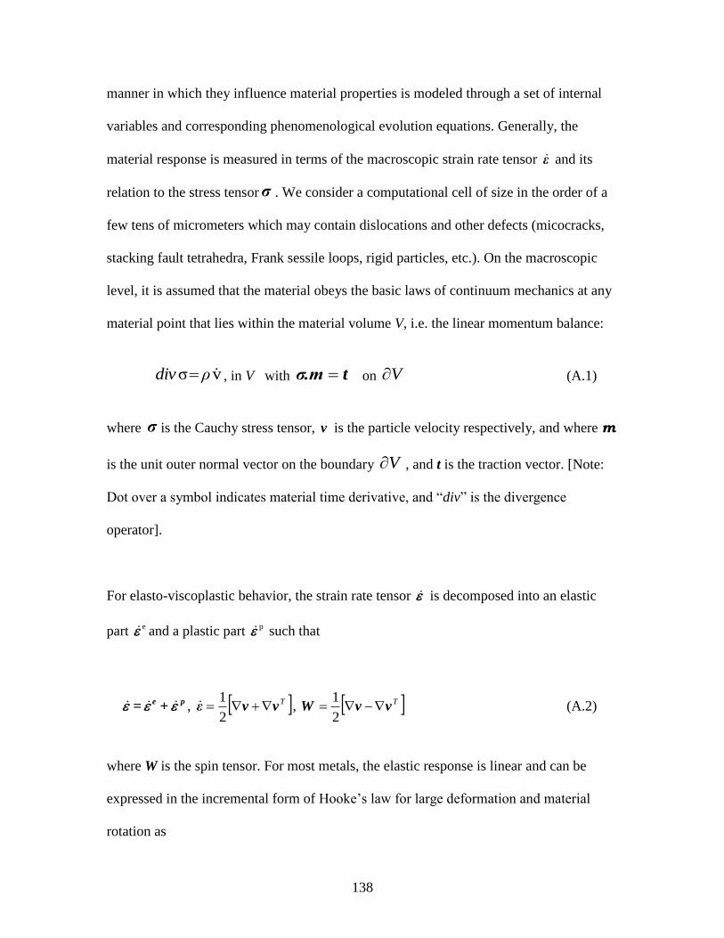
138

manner in which they influence material properties is modeled through a set of internal

variables and corresponding phenomenological evolution equations. Generally, the

material response is measured in terms of the macroscopic strain rate tensor ε and its

relation to the stress tensor σ . We consider a computational cell of size in the order of a

few tens of micrometers which may contain dislocations and other defects (micocracks,

stacking fault tetrahedra, Frank sessile loops, rigid particles, etc.). On the macroscopic

level, it is assumed that the material obeys the basic laws of continuum mechanics at any

material point that lies within the material volume V, i.e. the linear momentum balance:

vσ ρdiv , in V with tσ.m on V (A.1)

where σ is the Cauchy stress tensor, v is the particle velocity respectively, and where m

is the unit outer normal vector on the boundary V , and t is the traction vector. [Note:

Dot over a symbol indicates material time derivative, and “div” is the divergence

operator].

For elasto-viscoplastic behavior, the strain rate tensor is decomposed into an elastic

part e and a plastic part p such that

pe + = , T

vvε 2

1 , T

vvW 2

1 (A.2)

where W is the spin tensor. For most metals, the elastic response is linear and can be

expressed in the incremental form of Hooke‟s law for large deformation and material

rotation as

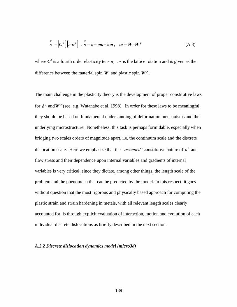
139

peo

ε-ε C = σ , σωωσσ= σo

, pω = W -W (A.3)

where Ce is a fourth order elasticity tensor, is the lattice rotation and is given as the

difference between the material spin W and plastic spin pW .

The main challenge in the plasticity theory is the development of proper constitutive laws

for p and pW (see, e.g. Watanabe et al, 1998). In order for these laws to be meaningful,

they should be based on fundamental understanding of deformation mechanisms and the

underlying microstructure. Nonetheless, this task is perhaps formidable, especially when

bridging two scales orders of magnitude apart, i.e. the continuum scale and the discrete

dislocation scale. Here we emphasize that the “assumed” constitutive nature of p and

flow stress and their dependence upon internal variables and gradients of internal

variables is very critical, since they dictate, among other things, the length scale of the

problem and the phenomena that can be predicted by the model. In this respect, it goes

without question that the most rigorous and physically based approach for computing the

plastic strain and strain hardening in metals, with all relevant length scales clearly

accounted for, is through explicit evaluation of interaction, motion and evolution of each

individual discrete dislocations as briefly described in the next section.

A.2.2 Discrete dislocation dynamics model (micro3d)

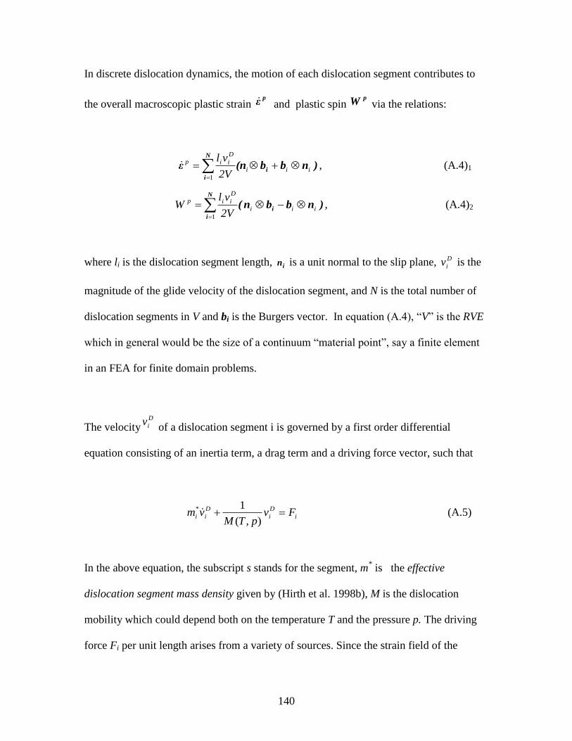
140

In discrete dislocation dynamics, the motion of each dislocation segment contributes to

the overall macroscopic plastic strain p

ε and plastic spin pW via the relations:

)nbb(nε i

N

i

iii

D

iip

2V

vl

1

, (A.4)1

)nbbn( i

N

i

iii

D

iip

2V

vlW

1

, (A.4)2

where li is the dislocation segment length, ni is a unit normal to the slip plane, D

iv is the

magnitude of the glide velocity of the dislocation segment, and N is the total number of

dislocation segments in V and bi is the Burgers vector. In equation (A.4), “V” is the RVE

which in general would be the size of a continuum “material point”, say a finite element

in an FEA for finite domain problems.

The velocityD

iv of a dislocation segment i is governed by a first order differential

equation consisting of an inertia term, a drag term and a driving force vector, such that

i

D

i

D

ii FvpTM

vm ),(

1* (A.5)

In the above equation, the subscript s stands for the segment, m* is the effective

dislocation segment mass density given by (Hirth et al. 1998b), M is the dislocation

mobility which could depend both on the temperature T and the pressure p. The driving

force Fi per unit length arises from a variety of sources. Since the strain field of the

141

dislocation varies as the inverse of the distance from the dislocation core, dislocations

interact among themselves over long distances, yielding a dislocation-dislocation

interaction force FD. A moving dislocation has to overcome local constraints such as the

Peierls stresses (i.e. lattice friction), FPeierls. The dislocation may encounter local obstacles

such as stacking fault tetrahedra, defect clusters and vacancies that interact with the

dislocation at short ranges, giving rise to a dislocation-obstacle interaction force FObstacle.

Furthermore, the internal strain field of randomly distributed local obstacles gives rise to

stochastic perturbations to the encountered dislocations, as compared with deterministic

forces such as the applied load. This stochastic stress field, or thermal force FThermal

arising from thermal fluctuations, also contributes to the spatial dislocation patterning in

the later deformation stages. Dislocations also interact with free surfaces, cracks, and

interfaces, giving rise to what is termed as image stresses or forces FImage. In addition, a

dislocation segment feels the effect of externally applied loads, FExternal, osmotic force

FOsmotic resulting from non-conservative motion of dislocation (climb) and its own self-

force FSelf. Adding all of these effects together yields the following expressions for the

driving force in (5).

ThermalOsmoticImageObstacleExternalSelfDPeirelsi FFFFFFFFF (A.6)

Exact expressions for each of these terms as well as treatment of short-range interactions

when two dislocations approach each other over a core distance, have been developed by

Zbib and co-workers, see for example (Zbib et al. 1996b), (Zbib et al. 1998), and

implemented into a dislocation dynamics software called micro3d.

142

In DD, once the velocity of the dislocation is calculated from (5), a search algorithm is

applied to check if there are any possible interactions with other dislocations within a

virtual area of the gliding dislocation. The length of the dislocation segment and the free

flight distance, define the virtual area gliding. The relation between the Burgers vector

and the slip systems of the two intersecting dislocation segments define the type of

interaction. When two dislocations intersect each other, one of the following interactions

occurs:

Annihilation: if the two dislocations have opposite Burgers vectors and glide in

the same slip plane.

Collinear annihilation: if the two dislocations have collinear Burgers vectors and

glide in intersecting slip planes, each plane being the cross-slip plane of the other.

Hirth lock: if the two dislocations have perpendicular Burgers vector and glide on

different slip planes.

Glissile junction: if the resulting Burgers vector is glissile on either of the planes.

Lomer Lock: if the resulting Burgers vector is sessile on either of the planes.

Screw dislocations may cross-slip to reduce internal stresses and to circumvent internal

obstacles. This process is a thermally activated process and, therefore, in DD it is

determined numerically using a Monte-Carlo type simulation as discussed by Kubin et al.

(1992), Rhee et al (1998) and Groh et al (2009). The probability P for a screw

dislocation segment of length L to cross-slip is given by

143

kT

VW

t

t

L

LP

*

00

exp (A.7)

where is a normalization factor, is the resolves shear stress on the slip plane, V is the

activation volume, W* is the activation energy to form a kink configuration in the cross-

slip plane as discussed by Rhee et al. (1998) plus constriction energy, t is the simulation

time step. k is the Boltzmann constant, T is the absolute temperature and is set to room

temperature; L0 = 1 µm and st 10 are reference values of length and time,

respectively.

A.2.3 Auxiliary Problem

The exact solution for the stress field of a dislocation segment, which is used among

other things to compute dislocation-dislocation interaction FD in equation (A.6), is known

for the case of infinite domain and linear elastic homogeneous materials, which is used in

DD codes. To account for surface effects in a finite domain, as well as for the case of

dislocations in linear elastic heterogeneous materials, one can use the principle of

superposition to solve for what is called above the image force FImage as briefly discussed

below.

A.2.3.1 Dislocation interaction with surfaces

The principle of superposition was used by (Van der Giessen and Needleman 1995) and

(Needleman 2000) for the 2D-DD case, and was extended to 3D-DD by (Fivel et al.

1998) and (Yasin et al. 2001) to correct for the actual boundary conditions, for both finite

144

domain and homogenous materials. Assuming that dislocation segments, dislocations

loops and any other internal defects with self induced stress [e.g. cracks can be modeled

as pile-ups of dislocation, (Demir and Zbib 2001)] are situated in a finite domain V

bounded by V and subjected to arbitrary external traction and displacement constraints,

then the stress field is given by the sum of two solutions:

ε*εε,u*uu,σσσ* (A.8)

where σ , and u are the stress, strain and displacement fields, respectively, caused

by the internal defects as if they were in an infinite domain, whereas *σ , * and *u are

the fields corresponding to the auxiliary problem satisfying the boundary conditions

V of part onV, on aauuttt

where at is the externally applied traction, and t is the traction induced on V by the

defects (dislocations) in the infinite domain problem. The traction - t on V results into

an image stress which is superimposed onto the dislocations segments, thus accounting

for surface-dislocation interaction.

A.2.3.2 Dislocations in Heterogeneous Materials

The superposition method described above for a dislocation in a finite and homogenous

domain has also been extended to the case of a dislocation in heterogeneous materials by

(Zbib and Diaz de la Rubia 2002). Briefly, suppose that domain V is divided into two

sub-domains V1 and V2 with domain V1 containing a set of dislocations. Then the stress

145

field induced by the dislocations and any externally applied stresses in both domains can

be constructed in terms of two solutions,

*, 1*1 (A.9)

where 1 and 1 are the stress and strain fields, respectively, caused by the

dislocations (the infinite solution) with the entire domain V having the same material

properties of domain V1 (homogenous solution) . The problem is now reduced to solving

for the auxiliary parts * and * in each of the domains. To do so, we first combine

equations (A.10) with Hooke‟s law for each of the sub-domains and obtain a new set of

elastic constitutive equations for each of the materials in each of the sub-domains as:

2

1e

1

21*21*e

2 ,;** Vin

Vin*,* 1

e

1

CCC

C

e

2

(A.10)

where eC1

and e

C2 are the elastic stiffness tensors in V1 and V2, respectively. The

“eigenstress” *21σ is due to the difference in material properties. The method yields very

accurate results when compared to known exact solution for simple dislocation

configurations, e.g. pure edge dislocation [(Akasheh et al. 2009)], and for a more general

case of a dislocation segment of arbitrary orientation and Burgers vectors [(Akarapu and

Zbib 2009)].

146

The three models described above, i.e. the DD model (micro3d), the elastic-

viscoplasticity model, and the auxiliary problem, are integrated into a unified system as

summarized in Figure A.1 yielding a hybrid multiscale model termed a “multiscale

dislocation dynamics plasticity -MDDP” which has the following two main features4:

1) It couples the continuum mechanics problem with discrete dislocation dynamics, and

2) it can deal with many possible boundary conditions, interfaces and dislocations in

heterogeneous materials.

A.3 Analysis of Plasticity and Deformation Mechanisms in Micropillar Compression

Test: Results and Discussions

We have considered cuboid shaped Cu specimens with thickness ranging from 0.2

microns to 2.5 microns. The length L is kept constant at 2.5 micron. The material

properties used in the simulation are summarized in Table 1. The values for the

dislocation mobility and stacking fault energy and their effect on the DD prediction have

been addressed in a number of articles, e.g. Kubin et al (1992), Rhee et al. (1998) Zbib et

al. (1998). In the compression experiments of single crystal Ni micropillars, Shan et. al

(2008) have observed an initial high dislocation density of the order of ~ 1015

(1/m2).

This density is almost three orders of magnitude larger than the typical density for a well

annealed material in bulk (~ 1012

/m2). They have also classified the defects into two

types: small loop-like and long arm like dislocation sources as depicted in Figure A.2a.

Kiener et al (2008) also argued that the partial removal of initial dislocation sources

during FIB milling produces single dislocation arms as depicted in Figure A.2a, and each

4micro3d and MDDP software with more details can be found at www.cmm.wsu.edu

http://www.cmm.wsu.edu/

147

can operate as depicted in Figure A.4a. Similar observations and models for dislocation

sources in micropillars have also been proposed by other investigators, e.g. Espinosa et

al. (2006), Tang et al. (2007, 2008) who also noted initial dislocation densities ranging

form 1013

to 1014

/m2. In the present work, an initial dislocation density of the order of

1013

(1/m2) with a random distribution of Frank-Read sources and jogged dislocation

arms extending from one surface to the other is considered as shown in the Figures

A.2a-c for the three cases of 0.5, 1.0 and 2.0 microns. The loading axis of the specimen

is along the <001> direction which is a high symmetry and low Schmid factor allowing

multi-slip. We impose the following boundary conditions.

Bottom surface:

In order to mimic as close as possible the experimental conditions in micropillar

compression test, in all the simulations, we keep the bottom of the specimen fixed such

that

ux=uy=uz=0, at Z=0

This, however, does not imply rigid boundary condition as far as the dislocations are

concerned. During the simulation, dislocations can penetrate the bottom surface and leave

the specimen. This condition is in conformity with the fact that the micropillars are

machined into a surface of a large-grained sheet and therefore, a micropillar and the

surface it sets on are of the same material, see for example, (Volkert and Lilleodden

148

2006). All other surfaces as far as the dislocations are concerned are free surfaces where

dislocation segments may annihilate.

Upper surface: Indenter-micropillar interface

The upper surface is subjected to a velocity vz so that the overall engineering strain rate

is kept constant at 100/s. i.e.

vz = L , at Z=L

Moreover, we consider two possible cases for the contact condition of the upper surface

with the loading apparatus:

Case 1: No friction, and therefore no additional constraints are imposed on the degrees of

freedom at the Z=L.

Case 2: Sticking friction, and therefore the additional following condition is imposed

ux=0, uy=0, at Z=L

A number of MDDP simulations were performed for various specimen sizes and

dislocation distributions with the boundary conditions as described above. The results are

summarized in Figures A.2-A.12. Below we discuss these results and present our

findings.

A.3.1 Effect of specimen size on yield stress

149

In this section, we present the stress-strain response for 0.2 to 2.5 microns thick

specimens under uniaxial compression at a constant strain rate of 100/s. Although the

strain rate used in the simulation is few orders of magnitude high when compared with

experiments, it does not have significant effect on the overall predictions in these types of

simulations, especially in the low strain rate regime where inertia effects are negligible

and the mobility is constant. The effect of both inertia and velocity-dependent mobility

on the overall mechanical behavior becomes important at very high strain rates (104/s and

above). These effects have been discussed in a number of articles, see e.g. Rhee et al

(1998), Hirth et al (1998), Zbib and Diaz de la Rubia (2002), Tang et al (2007),

Espinosa et al (2006). Figures A.2d-f show typical results of dislocation structures after

straining as predicted by MDDP. The predicted stress-strain curves are shown in Figure

A.3 for various specimen sizes. In qualitative terms, a typical stress-strain curve consists

of elastic regime followed by discrete strain bursts with considerable hardening. The

response in between two strain bursts has almost a linear elastic behavior. The predicted

stress-strain behavior is qualitatively similar in nature to that observed in experiments,

e.g. see (Volkert and Lilleodden 2006), Frick et al (2008), and Gruber et al (2008). At

higher strain rates, the stress-strain response is similar in nature but less serrated due to

the increased frequency of operation of dislocation arms. From these stress-strain curves,

we compute the yield stress at 0.02%, 0.2% and 0.4% strain offsets, and plotted the

results in Figure A. 4(a). The figure shows clearly significant size dependence for

specimens size less than 1.0 microns. The yield stress of 0.5 micron thick specimen is

almost 3-4 times the bulk yield stress. The simulation data at 0.02%, 0.2% and 0.4%

150

offset strain can be fitted to a modified source model (equation A.11) which we present in

section A.3.6 below. The simulation result at 0.02% and 0.4% offset strain is also plotted

in Figure A.4b. In the same figure we also plot experimental results extracted from the

literature, namely, from Greer and Nix (2006) for Au micropillars under compression,

Frick et al. (2008) for Ni micropillars under compression and Gruber et al. (2008) for Cu

free-standing thin films in tension. Form the experimental figures given in Greer and Nix

(2006) and Frick et al (2008), we estimated the flow stress at 3% (it was not possible to

extract data at lower offset). For the case of Cu, Gruber et al (2008) provide data for the

flow stress at 0.1% offset. Each experimental data set for the flow stress is normalized by

the shear modulus of the respective material and plotted in Figure A.4b. As it can be

seen from the figure, all the experimental data has the same trend in all cases, and for the

case of Cu it is quantitatively comparable to the simulation data. These results clearly

indicate that there is a considerable size effect even though the overall loading condition

is macroscopically homogenous. While under torsion and bending experiments, the

observed size effects can be attributed to the increase in the density of geometrically

necessary dislocations to accommodate for the strain gradients. There are no macroscopic

strain gradients in uniaxial compression and therefore, this effect can‟t be explained by

strain gradient theories. To understand this effect and the observed macroscopic response

of the sub-m specimens, a correlation between dislocation dynamics and macroscopic

response is presented in the following sub-section.

A.3.2 Correlation between microscopic mechanisms with macroscopic response

151

In micrometer to sub-m thick specimens, plastic deformation is mainly due to the

intermittent bowing out of dislocation arms, which are pinned inside the crystal at the

jogged portion on various slip planes, and at the point of their termination on the surface,

as illustrated in Figures A.5a-d. Each such mechanism of dislocation arm AB, ending on

the surface, bowing out intermittently and the annihilation of part of the arm BE and DF

by gliding towards the free surface under the effect of image stresses contributes to the

plastic deformation (see Figures A.5a-b). The dislocation arm changes its length and

curvature based on the geometry of the slip plane intersecting the free surface under the

influence of image and applied stress fields. The observed intermittency is caused by this

change in length and curvature of the dislocation arm during motion. In addition to the

dislocation arm mechanism, a dislocation arm ABC with AB portion on the (111 ) plane

and BC portion of the arm on the ( 111) plane with both of its ends on the free surface

acting as a spiral source also contributes to the strain bursts (see Figure A.5c). If the

stresses were homogeneous, these portions of arms under the dominance of image

stresses would have glided towards the line of intersection of the slip planes and

eventually disappeared on the surface (see Figure A.5c dotted lines). But due to the

heterogeneity of stress, the arms on the different planes are forced away from the surface

to act as a spiral source about the node B which is constrained to move along the line of

intersection. Thus, the dislocation arm operation and spiral sources are the major

contributors to the observed strain bursts.

The plastic deformation with intermittent dislocation bursts is quite prominent in the 0.5

micron thick specimen and gradually smoothens as the specimen size increases, similar to

152

the experimental observations. As it can be noticed, hardening, the slope of the stress-

strain response, significantly increases as the specimen size decreases (see Figure A.3).

The mechanisms responsible for the observed hardening in 0.2 to 0.5 m are

fundamentally different from those in the 1.0 to 2.5 m thick specimens. The dislocation

density is almost constant for 0.2 to 0.5 m thick specimens unlike a gradual increase in

1.0 to 2.5 m thick specimens (see Figure A.6). The dislocation density being constant in

sub-m specimens implies that the hardening is not conventional Taylor work hardening

caused by the storage of dislocations in a statistical sense. During the deformation of sub-

m specimens in which hardening is not caused by increase in dislocation density , there

are moments when the dislocation structure becomes immobile or stagnant, which

corresponds to elastic loading between strain bursts. Unlike the dislocation starvation

hypothesis, the elastic loading sections are due to stagnated dislocation structure as

opposed to the absence of dislocations in the specimen. The stagnation can be caused by

the pinning of dislocations by any one or a combination of the following mechanisms:

formation of entangled dislocation segments (Figure A.7), pinning of dislocations at

stress concentrations points (Figure A.9), and junction formation between interacting

dislocations (Figures A.8b). It is worth noting that the entangled structure is dependent

on the initial dislocation structure. The increase in stress required to mobilize the stagnant

dislocation structure can be explained by following reasons.

First of all, the dislocation arm under motion on the glide plane not only changes its

length and curvature but also forms entangled dislocation configurations which are hard

to mobilize (see Fig. 7a for such a typical structure). A schematic (Figure A.7b) is shown

153

to explain the typical process of formation of such dislocation structures. Consider a

dislocation arm AB on ( 111 ) with one end A pinned while the other end B on the free

surface having burgers vector along [ 101] and a dislocation CD of a Frank-Read source

on (111) with the same burgers vector as AB. During deformation, a segment pq of AB

on ( 111 ) aligns itself along the line of intersection to react with a similar segment rs of

CD on (111). This annihilation reaction of two screw segments along the line of

intersection of the slip planes results in two dislocation structures CqB and AsD. The

source length of the dislocation arm AB is now reduced to qB with motion of q end of the

dislocation restricted along the line of intersection of the slip planes. The formation of

dislocation structure CqB also reduces the source length of the CD to Cq. Moreover, the

motion of the dislocation end q is dependent on the motion of both Cq and qB. The

dislocation structure AsD also reduces the source length but it is much harder to mobilize

than CqB as both its ends are pinned on different slip planes. The formation of such

structures contributes to hardening to a considerable extent. Besides these entangled

dislocation structures, short range interactions of dislocations on different slip systems

resulted in the formation of jogs and junctions (see figure A.8b) have increased the

number of pinning sites which in turn contributed to the observed hardening. Upon

increase of stress to a critical value, these stagnant entangled dislocation structures AsD

and CqB become mobile and bow out to contribute to dislocation bursts after the

stagnation of dislocations.

As the bowing out of the dislocation arm is the primary mechanism for dislocation

motion, the yield stress of the specimen depends on the critical stress required to operate

154

a dislocation arm of maximum length. As the maximum length of the arm scales with the

sample thickness, the increase in yield stress with decrease in size relates inversely with

the length of the arm. Moreover, the number of such arms also scales with the specimen

thickness, which implies that the small sized specimens have fewer contributors to plastic

strain as opposed to large sized specimens. Thus, to accommodate for the imposed strain

rate, the frequency of activity of dislocation arms in the small sized specimens must be

greater to produce enough plastic strain, which in turn requires increase in stress. This is

a plausible explanation for the hardening observed in these sized specimens given the

absence of work hardening.

As noted above, the plastic deformation with intermittent dislocation bursts is quite

prominent in the 0.5 m thick specimen. There is a clear correlation among the

dislocation bursts, stress drops, the formation of junctions, and the activation of cross-slip

as shown in Figure A.8a-b as well as Figure A.6. Figure A.8b shows the number of

dislocations junctions as well as the number of cross-slip events; cross-slip took place

when the dislocations were pinned against a junction and or against a pinning site.

Furthermore, after the burst the dislocations that cross-slipped glide to the surface as

explained above in connection with Figure A.5, and as they terminate at the surface they

cause distortion and, therefore, a stress concentration as explained below in connection

with Figure A.9.

A.3.3 Effect of heterogeneous deformation

155

Figure A.9a, showing the deformed contour plots of effective plastic strain of the 0.5 m

thick specimen, exhibits localized plasticity along certain slip planes. At the top of the

specimen, the activity of the dislocation arm „1‟ is responsible for the plasticity on (111 )

slip planes and the activity of loop „2‟ near the surface resulted in localized deformation

and ledge formation at the surface as shown in Figure A.9b. The ledge results in a

heterogeneous stress field around the dislocation curve. Under a homogeneous stress

field, as would commonly be assumed for DD simulations that did not couple to FEM,

the loop would have been operating once the stress has reached a critical value. But as the

stress concentration at the surface is opposite to the attractive effect of image stresses, the

loop operates intermittently resulting in the observed serrated flow behavior. The

significant localization on ( 111 ) and (111 ) near the base also results in ledges and

subsequent stress concentrations at the surface. These heterogeneous stress fields assisted

the dislocation arms, shown in Figure A.5c, to act as spiral sources instead of annihilating

at the surface, as would occur under homogeneous stresses. As shown in the schematic

Figure A.9c, the dislocation arm AB gliding towards a stress concentrated spot at the

surface bows around that spot becomes stagnated. Until the stresses have reached a

certain level to overcome the effect of stress concentration and annihilate the dislocation

arm AB at the surface, dislocation arms CD and EF gliding towards the surface are also

stopped and a pile-up is formed. In this way, the stress concentration spots cause

dislocation arms to pile-up around them and in turn contribute to hardening (see the

snapshot shown in Figure A.9b.

156

To understand the importance and effect of heterogeneity, a comparison of stress-strain

response of 0.5 m thick specimen under constant strain rate compression using discrete

dislocation dynamics simulation (DD) was made with the response obtained using multi-

scale discrete dislocation simulation (MDDP). The results are shown in Figures A.10a-c.

In the constant strain rate dislocation dynamics simulation, the analysis is done solely at

the microscopic scale. During each loading time step, for the imposed strain, the stress is

computed homogenously over the entire domain (similar to the manner reported by (Tang

et al. 2008)). Under this homogeneous stress, the dislocations glide on the slip planes

during the loading time step and the plastic strain is computed from the collective motion

of the dislocations which is averaged over the entire domain. By doing the simulation

solely at the microscopic scale, the configuration change and, more importantly, its

influence on the dynamics of dislocations are not captured. Thus, as it can be seen from

the Fig. 10a, once the stress reaches a value which could activate the smallest dislocation

arm, the stress-strain response increases only slightly due to internal dislocation

interactions. This is not the case when performing the full MDDP analysis. As it can be

seen from Figure A.10a, once yielding begins the stress-strain curve exhibits more

pronounced serrated behavior with increasing stress levels and a more significant

hardening slope. More importantly, while the deformation field in the case the DD only

analysis is assumed to be homogenous, the MDDP analysis shows that the field is highly

heterogeneous as can be deduced from the inserts in Figure A.10a which show the

distribution of plastic strain for two boundary conditions (discussed in section A.3.5).

157

In this work, we are emphasizing that the heterogeneity of deformation and in turn the

stress distribution play a key role in capturing the observed hardening. The multi-scale

model, used in the present work, combines macroscopic and microscopic scales which

enables to take into account the effect of change in configuration and in turn the stress

heterogeneity on the dynamics of dislocations. Figures A.10b and A.10c clearly show

this effect, in terms of both evolution of dislocation density, and formation of dislocation

junctions, intersections, and cross-slip activities.

A.3.4 Effect of dislocation distribution

In a small volume at the sub-micron scale a relatively high dislocation density, say, on

the order of 1013

/m2, corresponds to only a limited number of dislocation segments

which may be distributed non-uniformly in the crystal, as shown in Figure A.2a. For the

same specimen with the same dislocation density, the dislocations can be spatially

rearranged in different ways, which yield different behavior. Towards this end, we have

done MDDP simulations with same dislocation density but different random

distributions. One of the two distributions is spatially heterogeneous with more

dislocation clustered at the base of the specimen whereas the other distribution has

dislocations homogeneously spaced over the entire specimen. The stress-strain response

of these two different distributions under uniaxial compression is shown in figure A.11.

As it can be seen from the figure A.11, for the case of heterogeneous distribution, there

are significant dislocation bursts as opposed to the case of homogenous distribution. In

the heterogeneous distribution, the proximity of dislocations is small enough for

158

interactions to form entangled dislocation structures. At a critical state of stress, the bow

out of these entangled structures leads to an avalanche of dislocations which occurs near

the bottom where the stresses are high because of boundary effects and where there is a

small cluster of dislocation sources. This leads to localized deformation as can be

deduced from the insert in Figure A.10. However, when the distribution is relatively

homogenous this behavior doesn‟t occur. We also note that in the case of homogenous

distribution, dislocations do not get pinned against each other as in the case of

heterogeneous distribution and therefore no cross-slip events take place and no

dislocation bursts are observed. Assumption of the existence of a few dislocation

sources, rather than a homogeneous array of sources, is supported by experiments in the

literature. Transmission electron microscopy of compression tests of ultra fine pillars

(smaller than the simulations in this current study by Shan et. al. (2008) showed that the

defects induced by machining pillars were prevalent, but rapidly removed during initial

contacts, leading to few, if any, sources and those are likely in the “bottom” of the pillar

where TEM observations are not possible. Kiener et. al. (2008) discuss the likelihood of

damage during micromachining of microtensile experiments, and we follow their

assumptions in this paper; there are few sources in these samples, but the sources do exist

and are positioned as individual heterogeneous sources.

A.3.5 Effect of boundary conditions

In this final section, we examine the effect of boundary conditions on the mechanical

behavior of the micropillars under compression, especially the condition on the upper

159

surface of the specimen. In all of the experiments on micropillars, the columns are

compressed using a nanoindentation apparatus. The conditions at upper surface will

depend on the type and the topological conditions of the indenter tip. Therefore, here we

examine two extreme cases: Case 1: No friction and Case 2: Sticking friction. The

results shown in Figure A.12 clearly illustrate that there is a significant effect on the

deformation behavior for the case of a 0.5 m size specimen with the same initial

dislocation distribution and density but under different boundary conditions. When the

upper surface is free to move, one slip system dominates and the deformation is localized

in two adjacent slip bands located towards the bottom end of the specimen while the

upper portion of the specimen glides freely over these bands and deforms elastically. On

the other hand, when the upper end is constrained two slip systems are activated and the

localization occurs towards the upper surface of the specimen. These results are

consistent with the experimental observations found in the literature, see for example,

(Greer and Nix 2005) and (Volkert and Lilleodden 2006). One last observation is that

when the dislocation density is relatively high and homogenous as is the case in Figure

A.10, the effect of the conditions on the upper surface is not as pronounced as can be

deduced from the two inserts in Figure A.10a. In this case, and because of the

abundance of dislocations, the deformation is not as highly localized as in the case shown

in Figure A.12.

160

A.3.6 A model for size effects in micro-samples

Assuming that the initial flow stress in micro-samples is determined by the size of a

single dislocation arm, we consider an arm with length equal to one-half of the size of the

specimen as depicted in Figure A.5a. One end of the arm is pinned at the center of the

crystal and the other end pinned on the surface lying on {111} slip plane. Under a

homogeneous stress state, the critical resolved shear stress to operate the arm with and

without the effect of image stresses is determined using MDDP. The critical resolved

shear stress is converted to uniaxial yield stress using a Schmid factor (m) of 0.422 and

plotted in Figure A.4a for different specimen sizes. As it can be seen from the figure, the

yield stress computed at 0.02% offset strain closely matches with the yield stress to

operate a single arm. This implies that the onset of plasticity in these micropillars is

mainly due to single arm operation with minimal effect of image stresses; the difference

between image-stress versus without image-stress is less that 10%. The flow stress y to

operate a single source of the type shown in Figure A.5a can be derived analytically from

the size of the dislocation source (source model; Foreman, 1967), which in this case is

equal to s/2, with s being the thickness of the micropillar (see also Kiener et al. 2008, and

Gruber et al 2008), and can be expressed as )2//()2/ln()2/( sbsby

, where is

a numerical constant in the order of unity. This relation can explain the onset of yielding

when the dislocation arm with the highest resolved shear stress operates freely without

obstacles and in a homogenous stress field. However, as discussed in this paper in

connection with the MDDP result, with increased plastic deformation, strain hardening

occurs (Figures A.3 and A.4a) which is attributed to two phenomena: dislocation

161

stagnation caused by the formation of an entangled dislocation structure, and the

formation of ledges. The dislocation entanglement effectively reduces the size of the

dislocation arm, and this effect can be introduced in the “source model” by introducing a

power term, i.e. 1/sn (Rhee et al., 1994). The ledge formation takes place as a result of

dislocation emerging on the surface, and this in turn results in a back stress which is

dependent on the surface energy and the size of the ledge and is inversely proportional to

the specimen size (Dewald et al, 1989). This leads us to propose the following model.

2 1 ln( ) 2 2;

2

y

n

s ss

m s s b

(A.11)

The first term quantifies the effect of source length but modified (power n<1) to account

for strain hardening as discussed above. (In the “source model” n=1). The second term

on the right hand side of equation (A.11) gives the effect of stress concentration due to

ledge formation, with being the surface energy (for Cu it is taken as 1.69 J m-2;

Dewald et al. 1989). It is assumed that the parameter is an integer measuring the

number of the dislocations that emerged on the surface to form the ledge, implying that

the size of the ledge increases proportionally to the number of the emerging dislocations.

The contribution of the ledge term in equation (A.11) becomes important as the specimen

size is decreased and as the size of the ledge increases with deformation. The two

parameters, n and , are thus functions of plastic strain. Their values are obtained by

fitting equation (A.11) to the MDDP numerical result for the yield stress evaluated at

0.02%, 0.2% and 0.4% offset strain; see Figure A.4a. While the value of n decreases with

increasing plastic strain, implying strain hardening due to pinning effects, the value of

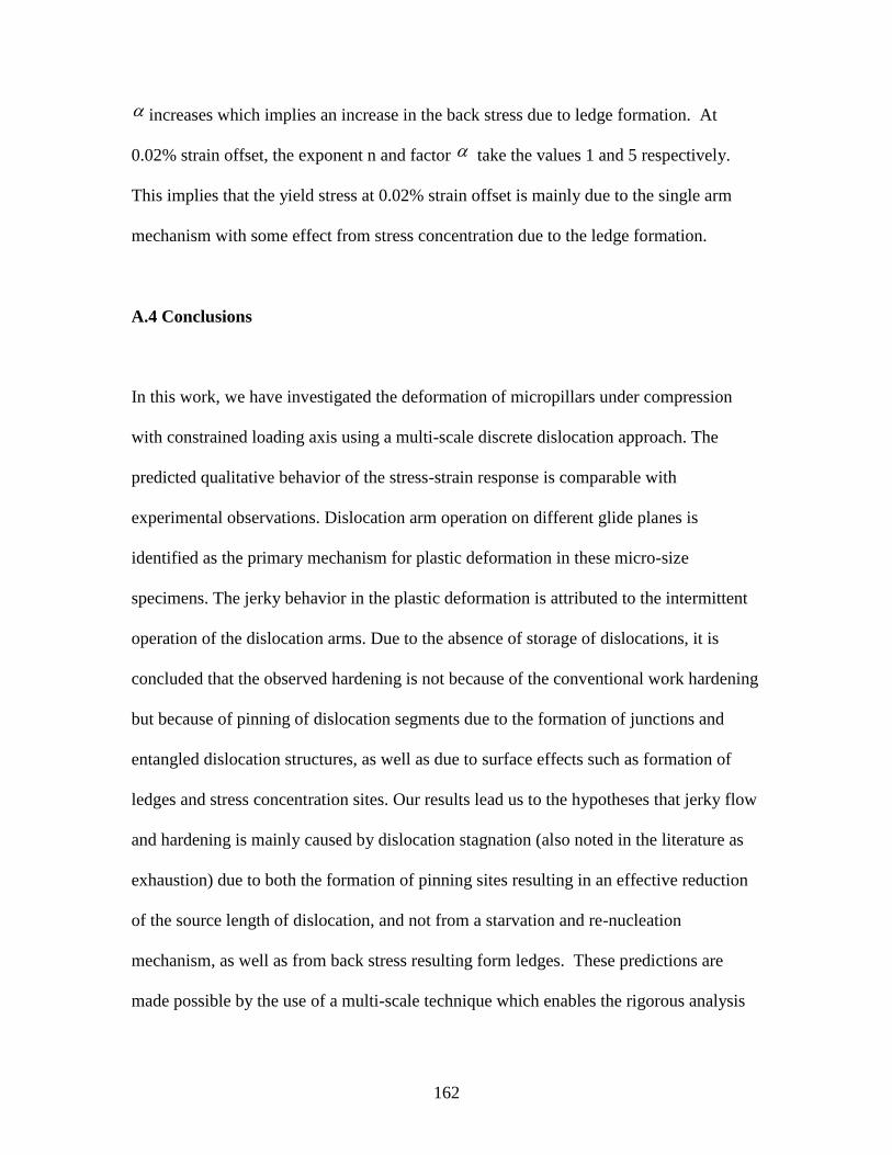
162

increases which implies an increase in the back stress due to ledge formation. At

0.02% strain offset, the exponent n and factor take the values 1 and 5 respectively.

This implies that the yield stress at 0.02% strain offset is mainly due to the single arm

mechanism with some effect from stress concentration due to the ledge formation.

A.4 Conclusions

In this work, we have investigated the deformation of micropillars under compression

with constrained loading axis using a multi-scale discrete dislocation approach. The

predicted qualitative behavior of the stress-strain response is comparable with

experimental observations. Dislocation arm operation on different glide planes is

identified as the primary mechanism for plastic deformation in these micro-size

specimens. The jerky behavior in the plastic deformation is attributed to the intermittent

operation of the dislocation arms. Due to the absence of storage of dislocations, it is

concluded that the observed hardening is not because of the conventional work hardening

but because of pinning of dislocation segments due to the formation of junctions and

entangled dislocation structures, as well as due to surface effects such as formation of

ledges and stress concentration sites. Our results lead us to the hypotheses that jerky flow

and hardening is mainly caused by dislocation stagnation (also noted in the literature as

exhaustion) due to both the formation of pinning sites resulting in an effective reduction

of the source length of dislocation, and not from a starvation and re-nucleation

mechanism, as well as from back stress resulting form ledges. These predictions are

made possible by the use of a multi-scale technique which enables the rigorous analysis

163

of non-uniform deformation of small scale specimens with realistic treatment of loading

and boundary conditions.

Acknowledgement

This work was supported by the Division of Materials Science and Engineering, Office of

Basic Energy Science at the U.S. Department of Energy under grant number DE-FG02-

07ER4635.

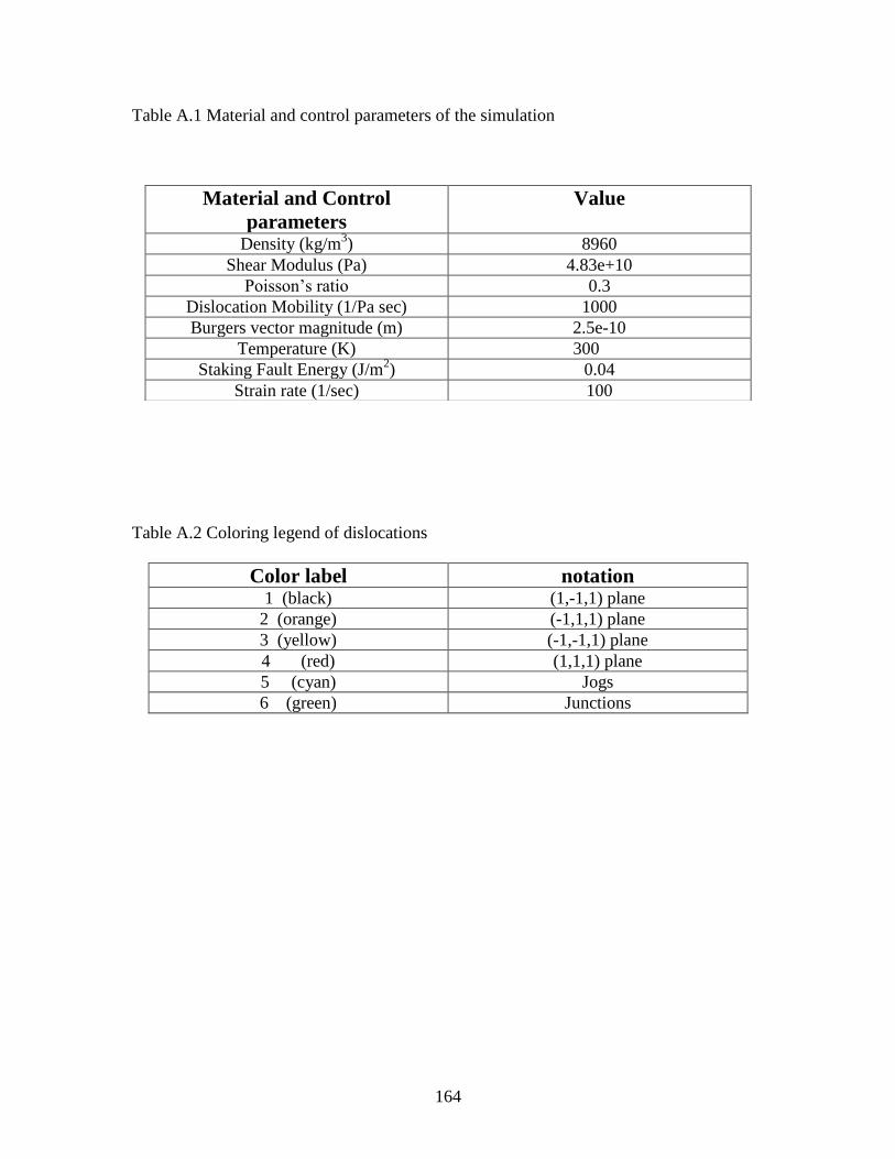
164

Table A.1 Material and control parameters of the simulation

Table A.2 Coloring legend of dislocations

Color label notation

1 (black) (1,-1,1) plane

2 (orange) (-1,1,1) plane

3 (yellow) (-1,-1,1) plane

4 (red) (1,1,1) plane

5 (cyan) Jogs

6 (green) Junctions

Material and Control

parameters

Value

Density (kg/m3) 8960

Shear Modulus (Pa) 4.83e+10

Poisson‟s ratio 0.3

Dislocation Mobility (1/Pa sec) 1000

Burgers vector magnitude (m) 2.5e-10

Temperature (K) 300

Staking Fault Energy (J/m2) 0.04

Strain rate (1/sec) 100

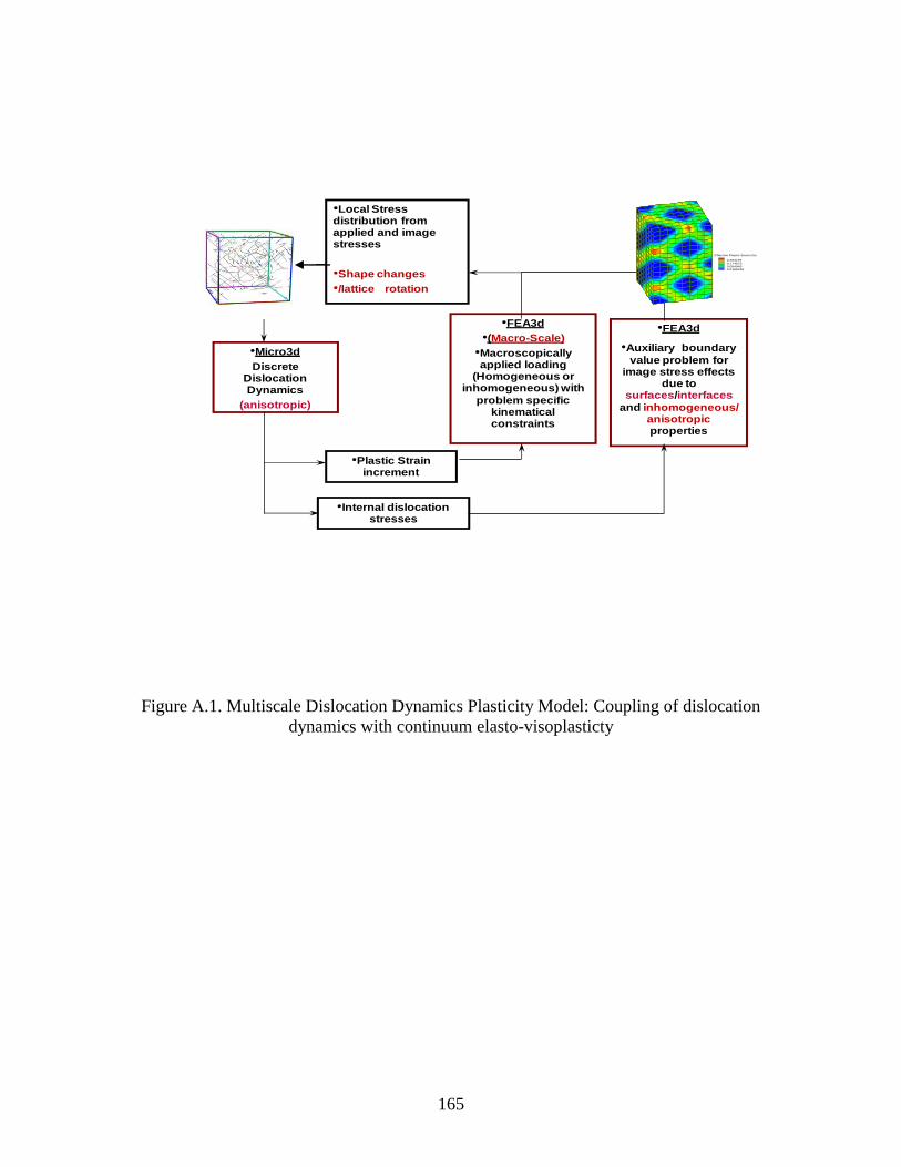
165

Figure A.1. Multiscale Dislocation Dynamics Plasticity Model: Coupling of dislocation

dynamics with continuum elasto-visoplasticty

•FEA3d

•(Macro-Scale)

•Macroscopically applied loading

(Homogeneous or inhomogeneous) with

problem specific kinematical constraints

•FEA3d

•Auxiliary boundary

value problem for image stress effects

due to surfaces/interfaces

and inhomogeneous/ anisotropic properties

•Local Stress distribution from applied and image stresses

•Shape changes

•/lattice rotation

•Micro3d

Discrete Dislocation Dynamics

(anisotropic)

•Plastic Strain increment

•Internal dislocation stresses

Effective Plastic Strain (%)

0.253197

0.174073

0.094949

0.0158248

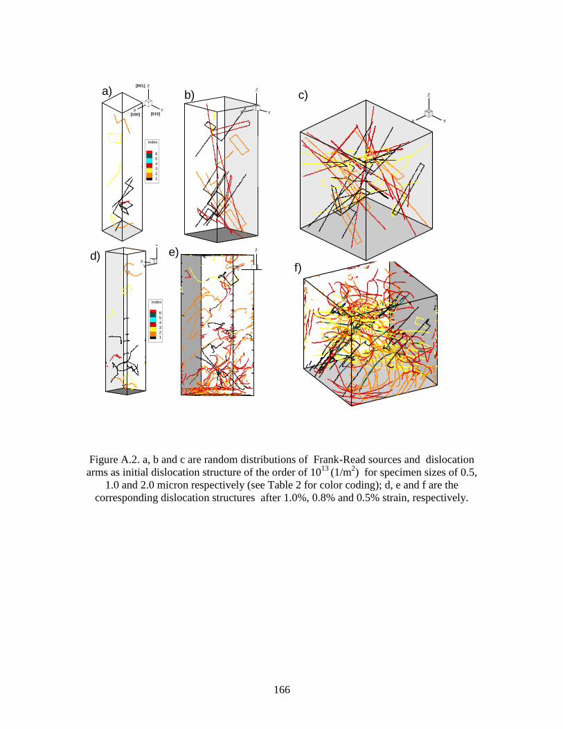
166

Figure A.2. a, b and c are random distributions of Frank-Read sources and dislocation

arms as initial dislocation structure of the order of 1013

(1/m2) for specimen sizes of 0.5,

1.0 and 2.0 micron respectively (see Table 2 for color coding); d, e and f are the

corresponding dislocation structures after 1.0%, 0.8% and 0.5% strain, respectively.

X

Z

Y

index

6

5

4

3

2

1

00

X Y

Z

index

6

5

4

3

2

1

[100] [010]

[001]

X Y

Z

index

6

5

4

3

2

1

XY

Z

index

6

5

4

3

2

1

XY

Z

index

6

5

4

3

2

1

X Y

Z

index

6

5

4

3

2

1

a) b) c)

d) e)

f)

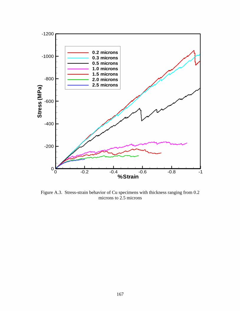
167

%Strain

Str

ess

(MP

a)

-1-0.8-0.6-0.4-0.20

-1200

-1000

-800

-600

-400

-200

0

0.2 microns

0.3 microns

0.5 microns

1.0 microns

1.5 microns

2.0 microns

2.5 microns

Figure A.3. Stress-strain behavior of Cu specimens with thickness ranging from 0.2

microns to 2.5 microns

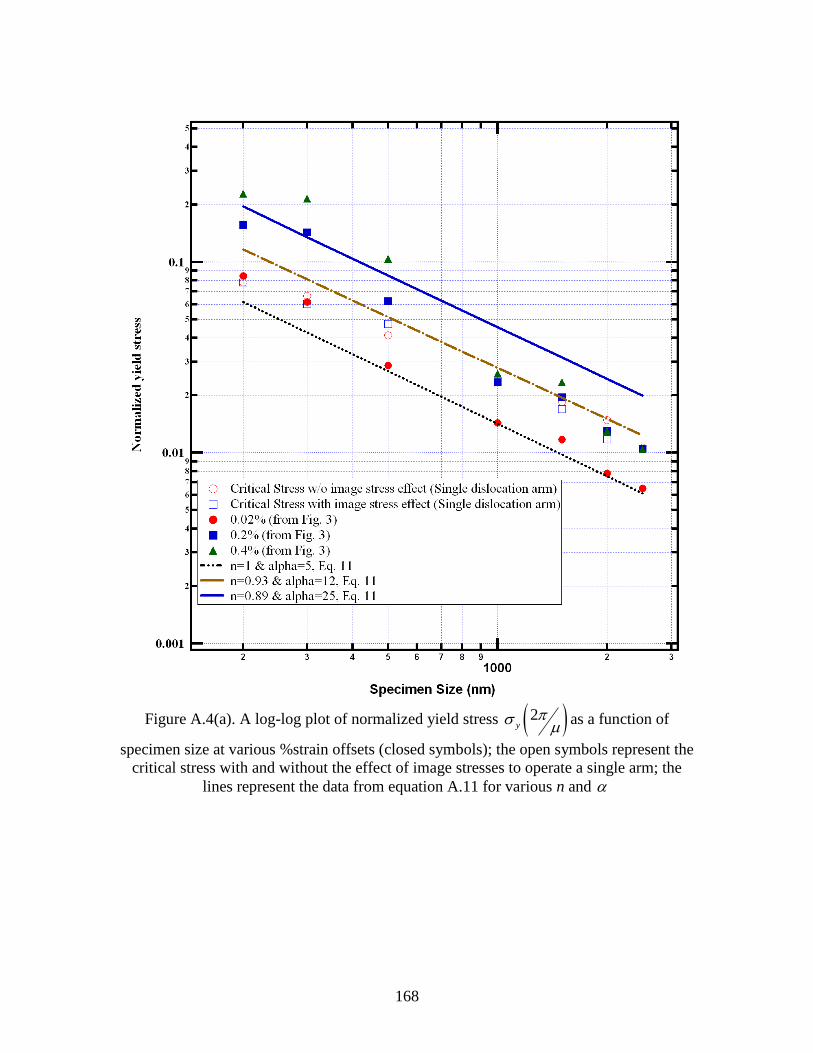
168

Figure A.4(a). A log-log plot of normalized yield stress 2y

as a function of

specimen size at various %strain offsets (closed symbols); the open symbols represent the

critical stress with and without the effect of image stresses to operate a single arm; the

lines represent the data from equation A.11 for various n and

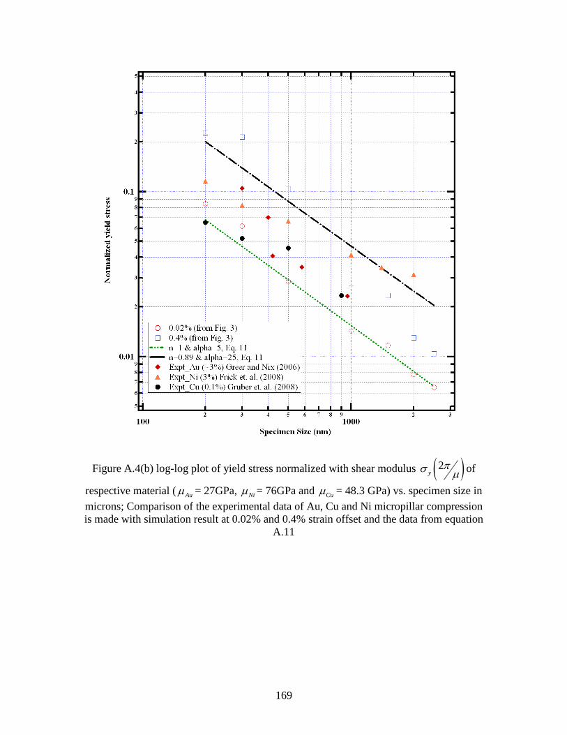
169

Figure A.4(b) log-log plot of yield stress normalized with shear modulus 2y

of

respective material ( Au = 27GPa, Ni = 76GPa and Cu = 48.3 GPa) vs. specimen size in

microns; Comparison of the experimental data of Au, Cu and Ni micropillar compression

is made with simulation result at 0.02% and 0.4% strain offset and the data from equation

A.11

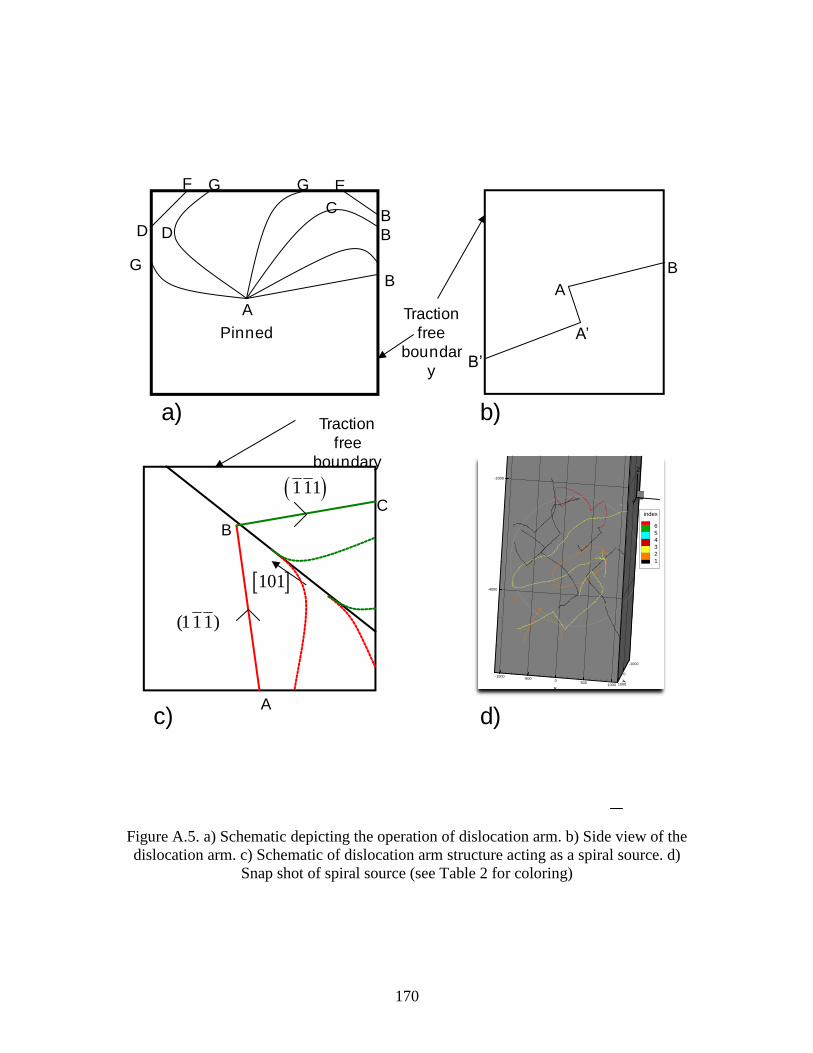
170

Figure A.5. a) Schematic depicting the operation of dislocation arm. b) Side view of the

dislocation arm. c) Schematic of dislocation arm structure acting as a spiral source. d)

Snap shot of spiral source (see Table 2 for coloring)

Traction

free

boundary

A

C

B

(111)

111

101

c)

X

-1000-500

0500

1000

Y

-1000

0

1000

-4000

-2000

Y

Z

index

6

5

4

3

2

1

A

B

B

BC

EGG

D

G

D

F

A

B

A’

B’

Pinned

Traction

free

boundar

y

a) b)

d)

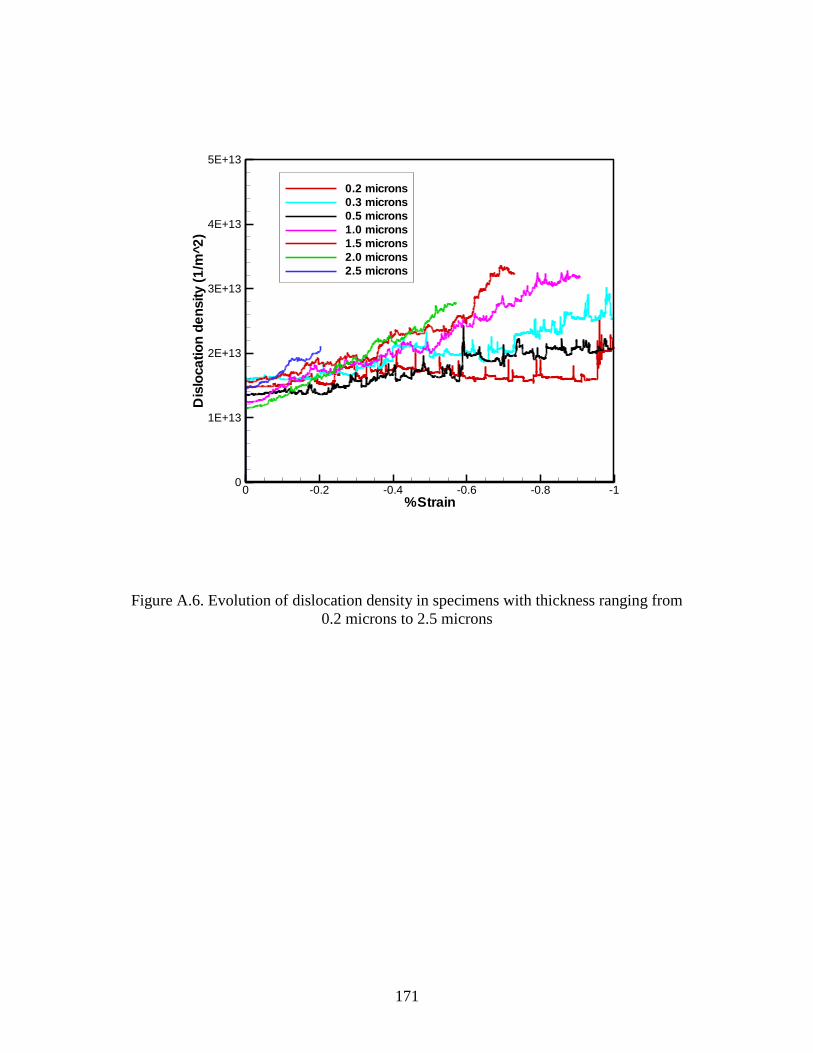
171

Figure A.6. Evolution of dislocation density in specimens with thickness ranging from

0.2 microns to 2.5 microns

%Strain

Dis

loca

tio

nd

en

sity

(1/m

^2

)

-1-0.8-0.6-0.4-0.200

1E+13

2E+13

3E+13

4E+13

5E+13

0.2 microns

0.3 microns

0.5 microns

1.0 microns

1.5 microns

2.0 microns

2.5 microns

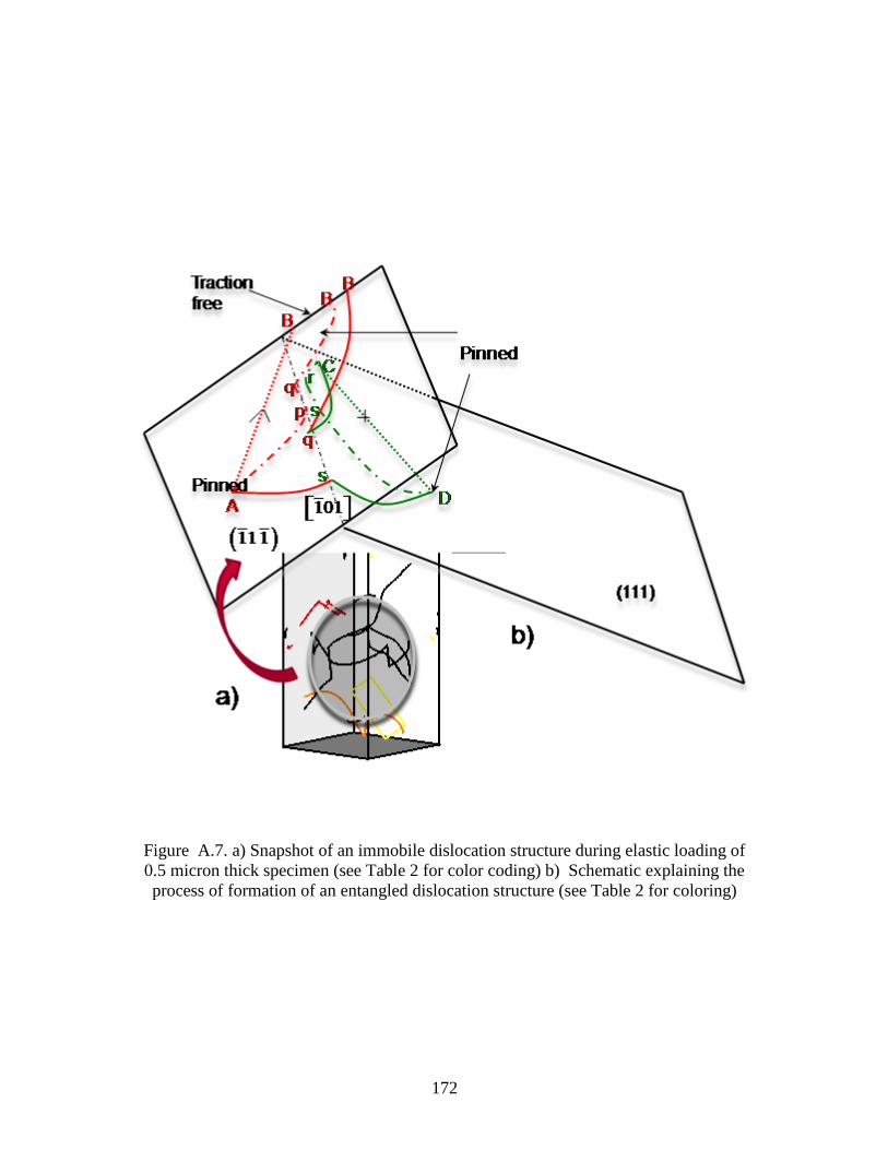
172

Figure A.7. a) Snapshot of an immobile dislocation structure during elastic loading of

0.5 micron thick specimen (see Table 2 for color coding) b) Schematic explaining the

process of formation of an entangled dislocation structure (see Table 2 for coloring)

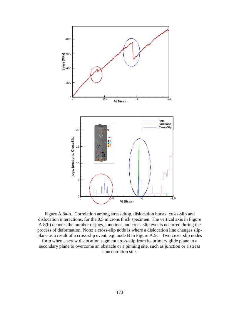
173

Figure A.8a-b. Correlation among stress drop, dislocation bursts, cross-slip and

dislocation interactions, for the 0.5 microns thick specimen. The vertical axis in Figure

A.8(b) denotes the number of jogs, junctions and cross-slip events occurred during the

process of deformation. Note: a cross-slip node is where a dislocation line changes slip-

plane as a result of a cross-slip event, e.g. node B in Figure A.5c. Two cross-slip nodes

form when a screw dislocation segment cross-slip from its primary glide plane to a

secondary plane to overcome an obstacle or a pinning site, such as junction or a stress

concentration site.

%Strain

Str

ess

(MP

a)

-1.5-1-0.50

-800

-600

-400

-200

0

%Strain

jog

s,ju

nctio

ns,C

rossS

lip

-1.5-1-0.500

5

10

15

20

jogs

junctions

CrossSlip

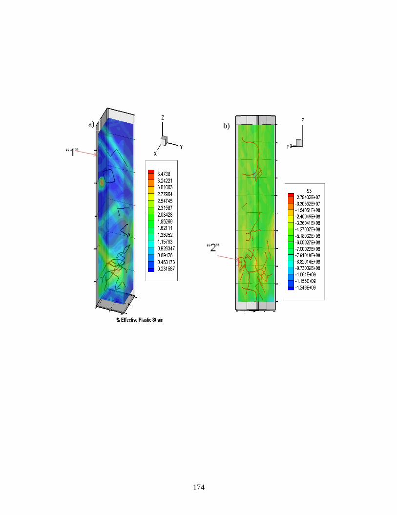
174

b) a)

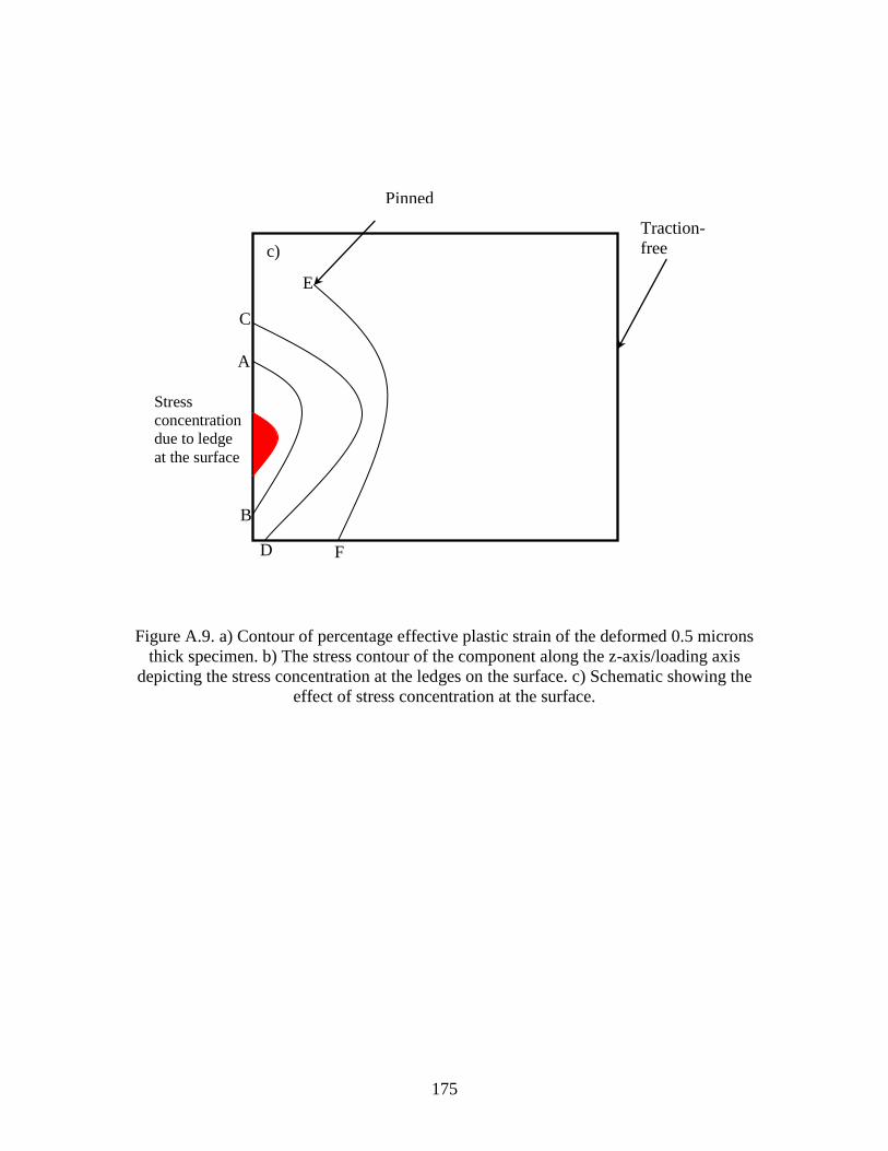
175

Figure A.9. a) Contour of percentage effective plastic strain of the deformed 0.5 microns

thick specimen. b) The stress contour of the component along the z-axis/loading axis

depicting the stress concentration at the ledges on the surface. c) Schematic showing the

effect of stress concentration at the surface.

A

B

C

D

E

F

Pinned

Traction-

free

boundary

Stress

concentration

due to ledge

at the surface

c)

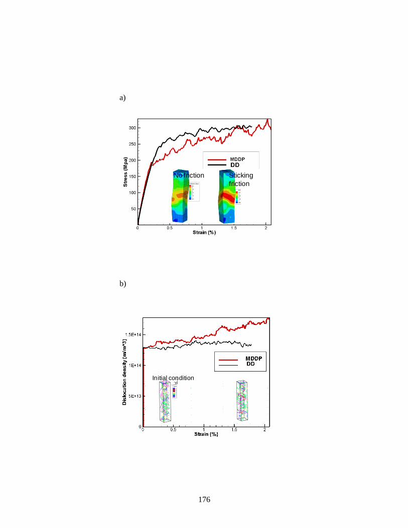
176

No friction Sticking

friction

timenow

dis

De

nsity

0 1E-06 2E-060

2E+13

4E+13

6E+13

8E+13

1E+14

1.2E+14

1.4E+14

1.6E+14

Frame 006 07 Oct 2008

timenow

dis

De

nsity

5E-07 1E-06

1.3E+14

1.35E+14

1.4E+14

timenow

Str

ess

0 1E-06 2E-06

-3E+08

-2.5E+08

-2E+08

-1.5E+08

-1E+08

-5E+07

Stress

Strain

Str

ess

-0.01-0.005

-3E+08

-2.5E+08

-2E+08

-1.5E+08

-1E+08

-5E+07

Frame 002 07 Oct 2008

Strain (%)

Str

ess

(Mp

a)

0 0.5 1 1.5 2

50

100

150

200

250

300

DDMDDP

X

Y

Z

X

Y

Z

Index

6

5

4

3

2

1

timenow

dis

De

nsity

0 1E-06 2E-060

2E+13

4E+13

6E+13

8E+13

1E+14

1.2E+14

1.4E+14

1.6E+14

Frame 006 07 Oct 2008

timenow

dis

De

nsity

5E-07 1E-06

1.3E+14

1.35E+14

1.4E+14

timenow

Str

ess

0 1E-06 2E-06

-3E+08

-2.5E+08

-2E+08

-1.5E+08

-1E+08

-5E+07

Stress

Strain

Str

ess

-0.01-0.005

-3E+08

-2.5E+08

-2E+08

-1.5E+08

-1E+08

-5E+07

Frame 002 07 Oct 2008

Strain (%)

Str

ess

(Mp

a)

0 0.5 1 1.5 2

50

100

150

200

250

300

DDMDDP

X

Y

Z

Initial condition

a)

b)

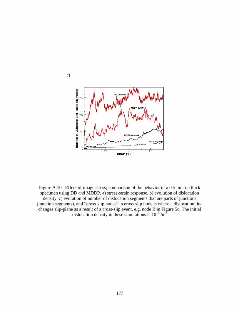
177

Figure A.10. Effect of image stress; comparison of the behavior of a 0.5 micron thick

specimen using DD and MDDP, a) stress-strain response, b) evolution of dislocation

density, c) evolution of number of dislocation segments that are parts of junctions

(junction segments), and “cross-slip nodes”, a cross-slip node is where a dislocation line

changes slip-plane as a result of a cross-slip event, e.g. node B in Figure 5c. The initial

dislocation density in these simulations is 1014

/m2

c)

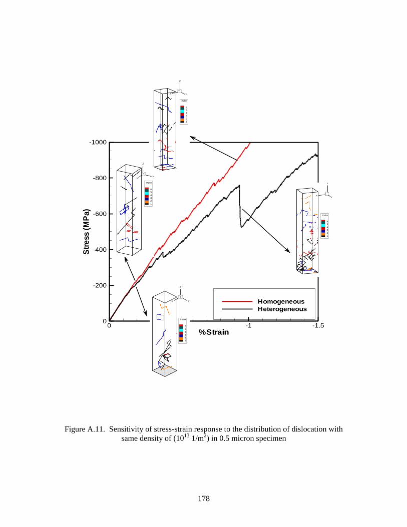
178

Figure A.11. Sensitivity of stress-strain response to the distribution of dislocation with

same density of (1013

1/m2) in 0.5 micron specimen

%Strain

Str

ess

(MP

a)

-1.5-1-0.50

-1000

-800

-600

-400

-200

0

Homogeneous

Heterogeneous

XY

Z

index

6

5

4

3

2

1

X

-1000

0

1000

X Y

Z

index

6

5

4

3

2

1

XY

Z

index

6

5

4

3

2

1

00

X Y

Z

index

6

5

4

3

2

1

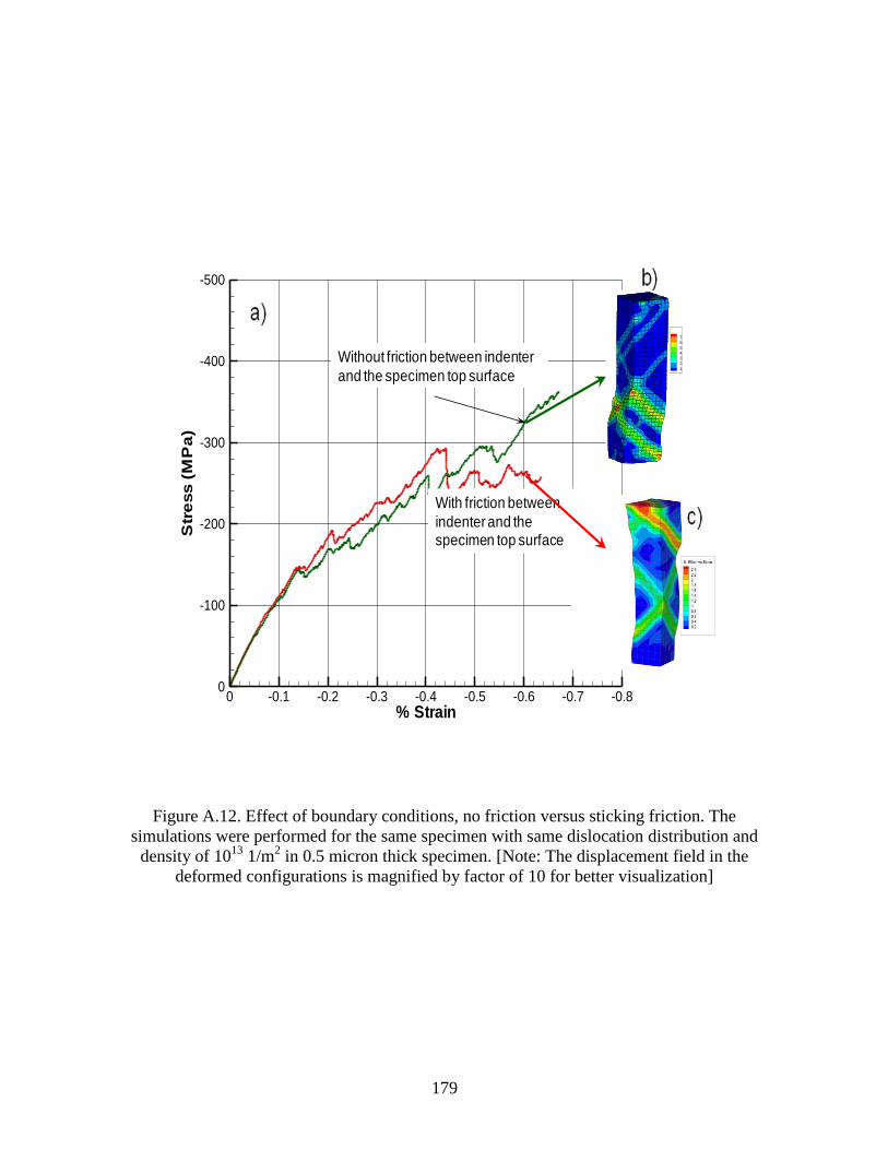
179

Figure A.12. Effect of boundary conditions, no friction versus sticking friction. The

simulations were performed for the same specimen with same dislocation distribution and

density of 1013

1/m2 in 0.5 micron thick specimen. [Note: The displacement field in the

deformed configurations is magnified by factor of 10 for better visualization]

(a)

(c)

% Strain

Str

ess

(MP

a)

-0.8-0.7-0.6-0.5-0.4-0.3-0.2-0.10

-500

-400

-300

-200

-100

0

With friction between

indenter and the specimen top surface

Without friction between indenter

and the specimen top surface

7

6

5

4

3

2

1

180

REFERENCES

Abu Al-Rub, R.K. and G.Z. Voyiadjis (2004), "Analytical and experimental

determination of the material intrinsic length scale of strain gradient plasticity theory

from micro- and nano-indentation experiments," Int. J. Plasticity, 20, 1139-1182.

Acharaya, A. and J.L. Bassani (2000), "Lattice Incompatibility and a Gradient Theory of

Crystal Plasticity," J. Mech. Phys. Solids, 48, 1565-1595.

Aifantis, E.C. (1984), "On the Microstructural Origin of Certain Inelastic Models,"

ASME J. Eng. Mat. Tech., 106, 326-330.

Akarapu, S., J. P. Hirth, and H. M. Zbib (2008), "Modeling and analysis of

disconnections in tilt walls," Scripta materialia, 59, 265-267.

Akarapu, S. and H.M. Zbib (2009), "Line-integral expressions for image stresses due to a

dislocation segment in isotropic joined half spaces," submitted.

Akasheh, F., H.M. Zbib, S. Akarupa, C. Overman, and D. Bahr (2009), "A multiscale

framework for modeling heterogeneity and interfaces in nanoscale metallic multilayered

composites," submitted.

Arsenlis, A. and D.M. Parks (1999), "Crystallographic aspects of geometrcially necessary

and statistically-stored dislocation density," Acta Metal., 47, 1597-1611.

Asaro, R.J. and D.M. Barnett (1973), "Appication of the geometrical theorems for

dislocations in anisotropic elastic media," in Computer Simulation for Materials

Applications.

Asaro, R.J. and A. Needleman (1985), "Texture development and strain hardening in

rate-dependent polycrystals," Acta Metall., 33, 923-.

Ashby, M.F. (1971), The Deformation of Plastically Non-Homogeneous Alloys.

Amsterdam: Elsevier.

Bahr, D.F. and W.W. Gerberich (1996), "Pile up and plastic zone size around

indentations," Met. Mater. Trans., 27A, 3793-3800.

Bahr, D.F., D.E. Kramer, and W.W. Gerberich (1998), "Non-linear deformation

mechanisms during nanoindentation," Acta Mater., 46, 176-182.

Bammann, D.J. (1984), "An Internal Variable Model of Viscoplasticity," Int. J.

Engineering Science, 8-10, 1041-.

181

Bammann, D.J. and E.C. Aifantis (1981), "On the Perfect Lattice-Dislocated State

Interaction," in Int. Symp. on Mechanical Behavior of Structured Media, A.P.S.

Selvadurai (Ed.). Amsterdam-Oxford-New York: Elsevier Scientific Publishing.

Barnett, D.M. (1972), "The precise evaluation of deivatives of the anisotropic elastic

Green's functions," Physica stat. sol. (b), 49, 741-748.

Barnett, D.M. and J Lothe (1973), "Synthesis of the sextic and the integral formalism for

dislocations, Green's functions, adn surface waves in anisotropic elastic solids," Physica

Norveg., 7, 13-19.

Benzerga, A.A. and N.F. Shaver (2006), "Size dependence of mechanical properties of

single crystals under uniform deformation," Scripts Mater., 54, 1937.

Brown, L.M. (1967), "A proof of Lothe's theorem," Philosophical Magazine, 15, 363-

370.

Clayton, J.D., D.L. McDowell, and D.J. Bammann (2006), "Modeling dislocations and

disclinations with finite micropolar elastoplasticity," Int. J. Plasticity, 22, 210-256.

Clemens, B. M., H. Kung, and S. A. Barnett (1999), "Structure and strength of

multilayers," MRS Bulletin, 24 (2), 20-26.

Demir, I. and H. M. Zbib (2001), "A Mesoscopic Model for Inelastic Deformation and

Damage," Int. J. Enger. Science, 39, 1597-1615.

Deshphande, V.S., A. Needleman, and E. Van der Giessen (2005), "Plasticity size effects

in tension and compression of single crystals," J. Mech. Phys. Solids, 53, 2661.

Dillon, O.W. and J. Kratochvil (1970), "A Strain Gradient Theory of Plasticity," Int. J.

Solids Structures, 6, 1513-1533.

Dimiduk, D.M., M.D. Uchic, and T.A. Parthasarathy (2005), "Size-affected single slip

behavior of pure nickel microcrystals," Acta Mater., 53, 4065.

Eshelby, J.D., W.T. Read, and W. Shockely (1953), "Anisotropic elasticity with

applications to dislocation theory," Acta Metall., 1, 251-259.

Fivel, M.C., C.F. Roberston, G. Canova, and L. Bonlanger (1998), "Three-Dimensional

Modeling of Indent-Induced Plastic Zone at a Mesocale," Acta Mater, 46 (17), 6183-

6194.

Fleck, N.A. and J.W. Hutchinson (2001), "A reformulation of strain gradient plasticity,"

Journal of Mechanics and Physics of Solids, 49, 2245-2271.

182

Fleck, N.A., G.M. Muller, M.F. Ashby, and J.W. Hutchinson (1994), "Strain Gradient

Plasticity: Theory and Experiment," Acta Metall. Mater., 42, 475-487.

Frick, C.P., B.G. Clark, S. Orso, A.S. Schneider, and E. Artz (2008), "Size effect on

strength and strain hardening of small-scale [111] nickel compression pillars," Mater. Sci.

Engg. A.

Greer, J.R. and W.D. Nix (2006), "Nanoscale gold pillars strengthened through

dislocation starvation," Phys. Rev.B, 73, 245210.

Greer, J.R. and W.D. Nix (2005), "Size dependence of mechanical properties of gold at

the sub-micron scale," Appli. Phys. A, 80, 1625-1629.

Grohm, S., E.B. Marin, M.F. Horstemeyer, and H.M. Zbib (2008), "Multiscale Modeling

of Plasticity in an Aluminum Single Crystal," Int. J. Plasticity, In press.

Gurtin, M.E. (2000), "On the plasticity of single crystal viscoplasticity that accounts for

geometrically necessary dislocations," International Journal of Plasticity, 19 (47-90).

Han, X. and N.M. Ghoniem (2005), "Stress field and interaction forces of dislocations in

anisotropic multilayer thin films," Philosophical Magazine, 85 (11), 1205-1225.

Head, A.K. (1953a), "Edge dislocations in inhomogeneous media," Proceedings of Royal

Soceity B, 66, 793-801.

Head, A.K. (1953b), "Interaction of dislocations and boundaries," Philosophical

Magazine, 44, 92-98.

Hirth, J. P. and R.W. Ballufi (1973), "On the grain boundary dislocations and ledges,"

Acta Metall., 21, 929-942.

Hirth, J. P., R.C. Pond, and J Lothe (2006), "Disconnections in tilt walls," Acta Mater.,

54, 4237-4245.

Hirth, J. P., H. M. Zbib, and J Lothe (1998a), "Forces on High Velocity Dislocations,"

Modeling and Simulations in Materials Science and Engineering, 6, 165-169.

Hirth, J.P., H.M. Zbib, and J. Lothe (1998b), " Forces on High Velocity Dislocations,"

Modeling & Simulations in Maters. Sci. & Enger., 6, 165-169.

Hirth, John Price and Jens Lothe (1982), Theory of dislocations (2nd ed.). New York:

Wiley.

Horstemeyer, M.F. and M.I. Baskes (1999), "Atomistic finite deformation simulations: A

discussion on length scale effects in relation to mechanical stresses," ASME-Journal of

Engineering Materials and Technology, 121, 114-119.

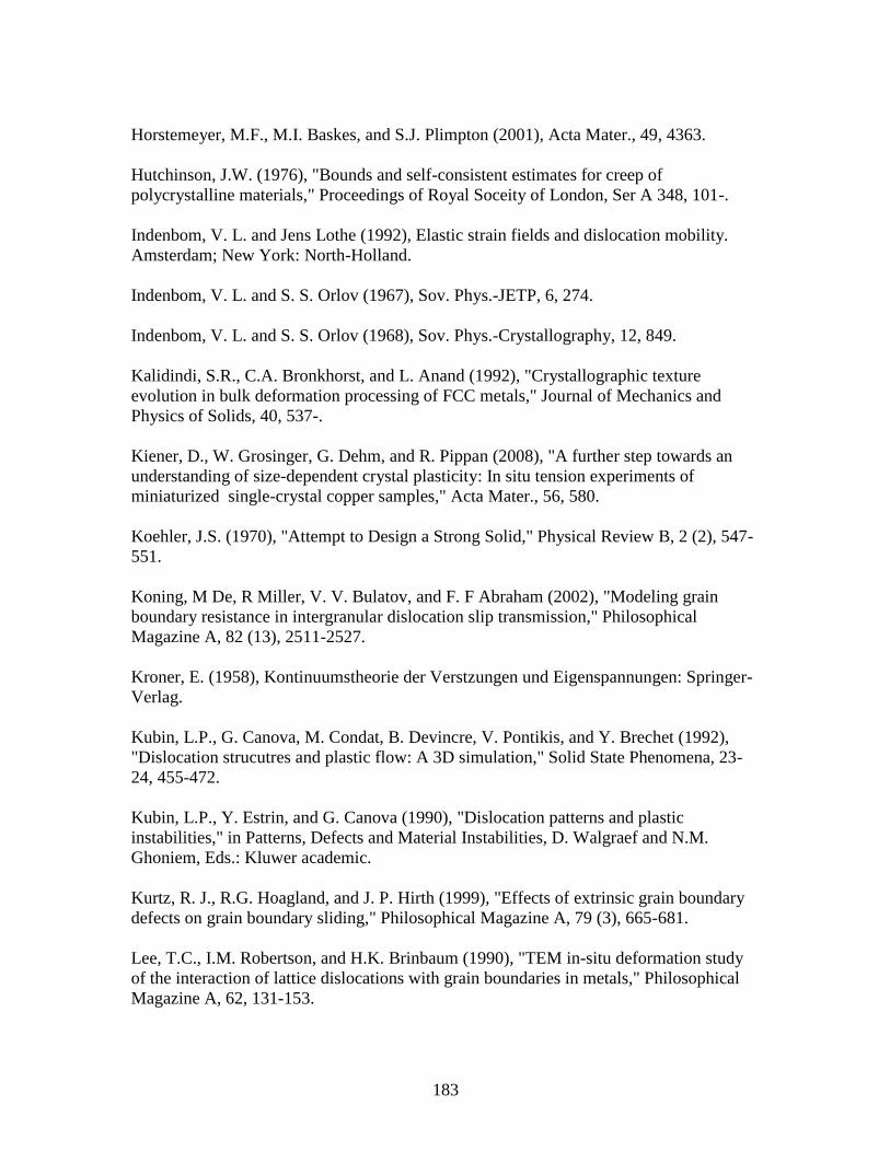
183

Horstemeyer, M.F., M.I. Baskes, and S.J. Plimpton (2001), Acta Mater., 49, 4363.

Hutchinson, J.W. (1976), "Bounds and self-consistent estimates for creep of

polycrystalline materials," Proceedings of Royal Soceity of London, Ser A 348, 101-.

Indenbom, V. L. and Jens Lothe (1992), Elastic strain fields and dislocation mobility.

Amsterdam; New York: North-Holland.

Indenbom, V. L. and S. S. Orlov (1967), Sov. Phys.-JETP, 6, 274.

Indenbom, V. L. and S. S. Orlov (1968), Sov. Phys.-Crystallography, 12, 849.

Kalidindi, S.R., C.A. Bronkhorst, and L. Anand (1992), "Crystallographic texture

evolution in bulk deformation processing of FCC metals," Journal of Mechanics and

Physics of Solids, 40, 537-.

Kiener, D., W. Grosinger, G. Dehm, and R. Pippan (2008), "A further step towards an

understanding of size-dependent crystal plasticity: In situ tension experiments of

miniaturized single-crystal copper samples," Acta Mater., 56, 580.

Koehler, J.S. (1970), "Attempt to Design a Strong Solid," Physical Review B, 2 (2), 547-

551.

Koning, M De, R Miller, V. V. Bulatov, and F. F Abraham (2002), "Modeling grain

boundary resistance in intergranular dislocation slip transmission," Philosophical

Magazine A, 82 (13), 2511-2527.

Kroner, E. (1958), Kontinuumstheorie der Verstzungen und Eigenspannungen: Springer-

Verlag.

Kubin, L.P., G. Canova, M. Condat, B. Devincre, V. Pontikis, and Y. Brechet (1992),

"Dislocation strucutres and plastic flow: A 3D simulation," Solid State Phenomena, 23-

24, 455-472.

Kubin, L.P., Y. Estrin, and G. Canova (1990), "Dislocation patterns and plastic

instabilities," in Patterns, Defects and Material Instabilities, D. Walgraef and N.M.

Ghoniem, Eds.: Kluwer academic.

Kurtz, R. J., R.G. Hoagland, and J. P. Hirth (1999), "Effects of extrinsic grain boundary

defects on grain boundary sliding," Philosophical Magazine A, 79 (3), 665-681.

Lee, T.C., I.M. Robertson, and H.K. Brinbaum (1990), "TEM in-situ deformation study

of the interaction of lattice dislocations with grain boundaries in metals," Philosophical

Magazine A, 62, 131-153.

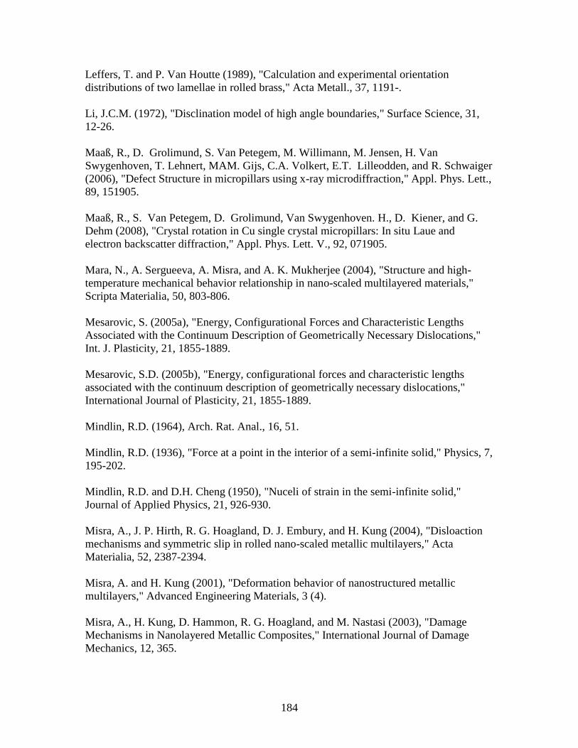
184

Leffers, T. and P. Van Houtte (1989), "Calculation and experimental orientation

distributions of two lamellae in rolled brass," Acta Metall., 37, 1191-.

Li, J.C.M. (1972), "Disclination model of high angle boundaries," Surface Science, 31,

12-26.

Maaß, R., D. Grolimund, S. Van Petegem, M. Willimann, M. Jensen, H. Van

Swygenhoven, T. Lehnert, MAM. Gijs, C.A. Volkert, E.T. Lilleodden, and R. Schwaiger

(2006), "Defect Structure in micropillars using x-ray microdiffraction," Appl. Phys. Lett.,

89, 151905.

Maaß, R., S. Van Petegem, D. Grolimund, Van Swygenhoven. H., D. Kiener, and G.

Dehm (2008), "Crystal rotation in Cu single crystal micropillars: In situ Laue and

electron backscatter diffraction," Appl. Phys. Lett. V., 92, 071905.

Mara, N., A. Sergueeva, A. Misra, and A. K. Mukherjee (2004), "Structure and high-

temperature mechanical behavior relationship in nano-scaled multilayered materials,"

Scripta Materialia, 50, 803-806.

Mesarovic, S. (2005a), "Energy, Configurational Forces and Characteristic Lengths

Associated with the Continuum Description of Geometrically Necessary Dislocations,"

Int. J. Plasticity, 21, 1855-1889.

Mesarovic, S.D. (2005b), "Energy, configurational forces and characteristic lengths

associated with the continuum description of geometrically necessary dislocations,"

International Journal of Plasticity, 21, 1855-1889.

Mindlin, R.D. (1964), Arch. Rat. Anal., 16, 51.

Mindlin, R.D. (1936), "Force at a point in the interior of a semi-infinite solid," Physics, 7,

195-202.

Mindlin, R.D. and D.H. Cheng (1950), "Nuceli of strain in the semi-infinite solid,"

Journal of Applied Physics, 21, 926-930.

Misra, A., J. P. Hirth, R. G. Hoagland, D. J. Embury, and H. Kung (2004), "Disloaction

mechanisms and symmetric slip in rolled nano-scaled metallic multilayers," Acta

Materialia, 52, 2387-2394.

Misra, A. and H. Kung (2001), "Deformation behavior of nanostructured metallic

multilayers," Advanced Engineering Materials, 3 (4).

Misra, A., H. Kung, D. Hammon, R. G. Hoagland, and M. Nastasi (2003), "Damage

Mechanisms in Nanolayered Metallic Composites," International Journal of Damage

Mechanics, 12, 365.

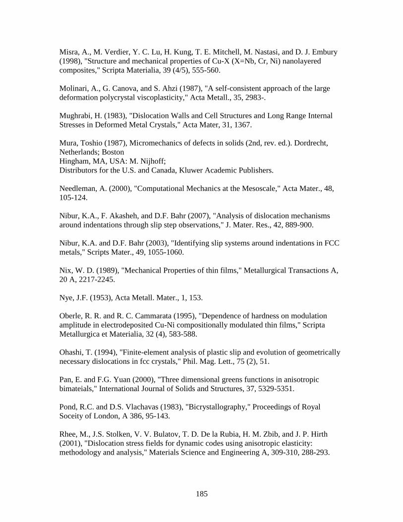
185

Misra, A., M. Verdier, Y. C. Lu, H. Kung, T. E. Mitchell, M. Nastasi, and D. J. Embury

(1998), "Structure and mechanical properties of Cu-X (X=Nb, Cr, Ni) nanolayered

composites," Scripta Materialia, 39 (4/5), 555-560.

Molinari, A., G. Canova, and S. Ahzi (1987), "A self-consistent approach of the large

deformation polycrystal viscoplasticity," Acta Metall., 35, 2983-.

Mughrabi, H. (1983), "Dislocation Walls and Cell Structures and Long Range Internal

Stresses in Deformed Metal Crystals," Acta Mater, 31, 1367.

Mura, Toshio (1987), Micromechanics of defects in solids (2nd, rev. ed.). Dordrecht,

Netherlands; Boston

Hingham, MA, USA: M. Nijhoff;

Distributors for the U.S. and Canada, Kluwer Academic Publishers.

Needleman, A. (2000), "Computational Mechanics at the Mesoscale," Acta Mater., 48,

105-124.

Nibur, K.A., F. Akasheh, and D.F. Bahr (2007), "Analysis of dislocation mechanisms

around indentations through slip step observations," J. Mater. Res., 42, 889-900.

Nibur, K.A. and D.F. Bahr (2003), "Identifying slip systems around indentations in FCC

metals," Scripts Mater., 49, 1055-1060.

Nix, W. D. (1989), "Mechanical Properties of thin films," Metallurgical Transactions A,

20 A, 2217-2245.

Nye, J.F. (1953), Acta Metall. Mater., 1, 153.

Oberle, R. R. and R. C. Cammarata (1995), "Dependence of hardness on modulation

amplitude in electrodeposited Cu-Ni compositionally modulated thin films," Scripta

Metallurgica et Materialia, 32 (4), 583-588.

Ohashi, T. (1994), "Finite-element analysis of plastic slip and evolution of geometrically

necessary dislocations in fcc crystals," Phil. Mag. Lett., 75 (2), 51.

Pan, E. and F.G. Yuan (2000), "Three dimensional greens functions in anisotropic

bimateials," International Journal of Solids and Structures, 37, 5329-5351.

Pond, R.C. and D.S. Vlachavas (1983), "Bicrystallography," Proceedings of Royal

Soceity of London, A 386, 95-143.

Rhee, M., J.S. Stolken, V. V. Bulatov, T. D. De la Rubia, H. M. Zbib, and J. P. Hirth

(2001), "Dislocation stress fields for dynamic codes using anisotropic elasticity:

methodology and analysis," Materials Science and Engineering A, 309-310, 288-293.

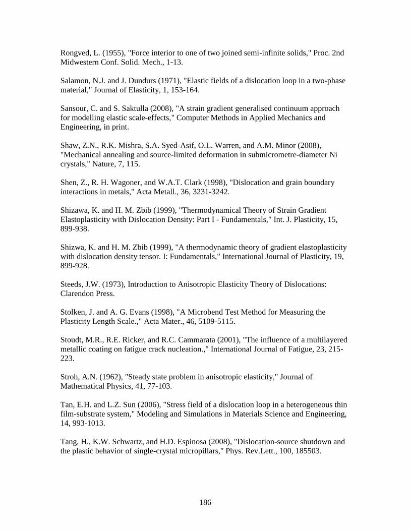
186

Rongved, L. (1955), "Force interior to one of two joined semi-infinite solids," Proc. 2nd

Midwestern Conf. Solid. Mech., 1-13.

Salamon, N.J. and J. Dundurs (1971), "Elastic fields of a dislocation loop in a two-phase

material," Journal of Elasticity, 1, 153-164.

Sansour, C. and S. Saktulla (2008), "A strain gradient generalised continuum approach

for modelling elastic scale-effects," Computer Methods in Applied Mechanics and

Engineering, in print.

Shaw, Z.N., R.K. Mishra, S.A. Syed-Asif, O.L. Warren, and A.M. Minor (2008),

"Mechanical annealing and source-limited deformation in submicrometre-diameter Ni

crystals," Nature, 7, 115.

Shen, Z., R. H. Wagoner, and W.A.T. Clark (1998), "Dislocation and grain boundary

interactions in metals," Acta Metall., 36, 3231-3242.

Shizawa, K. and H. M. Zbib (1999), "Thermodynamical Theory of Strain Gradient

Elastoplasticity with Dislocation Density: Part I - Fundamentals," Int. J. Plasticity, 15,

899-938.

Shizwa, K. and H. M. Zbib (1999), "A thermodynamic theory of gradient elastoplasticity

with dislocation density tensor. I: Fundamentals," International Journal of Plasticity, 19,

899-928.

Steeds, J.W. (1973), Introduction to Anisotropic Elasticity Theory of Dislocations:

Clarendon Press.

Stolken, J. and A. G. Evans (1998), "A Microbend Test Method for Measuring the

Plasticity Length Scale.," Acta Mater., 46, 5109-5115.

Stoudt, M.R., R.E. Ricker, and R.C. Cammarata (2001), "The influence of a multilayered

metallic coating on fatigue crack nucleation.," International Journal of Fatigue, 23, 215-

223.

Stroh, A.N. (1962), "Steady state problem in anisotropic elasticity," Journal of

Mathematical Physics, 41, 77-103.

Tan, E.H. and L.Z. Sun (2006), "Stress field of a dislocation loop in a heterogeneous thin

film-substrate system," Modeling and Simulations in Materials Science and Engineering,

14, 993-1013.

Tang, H., K.W. Schwartz, and H.D. Espinosa (2008), "Dislocation-source shutdown and

the plastic behavior of single-crystal micropillars," Phys. Rev.Lett., 100, 185503.

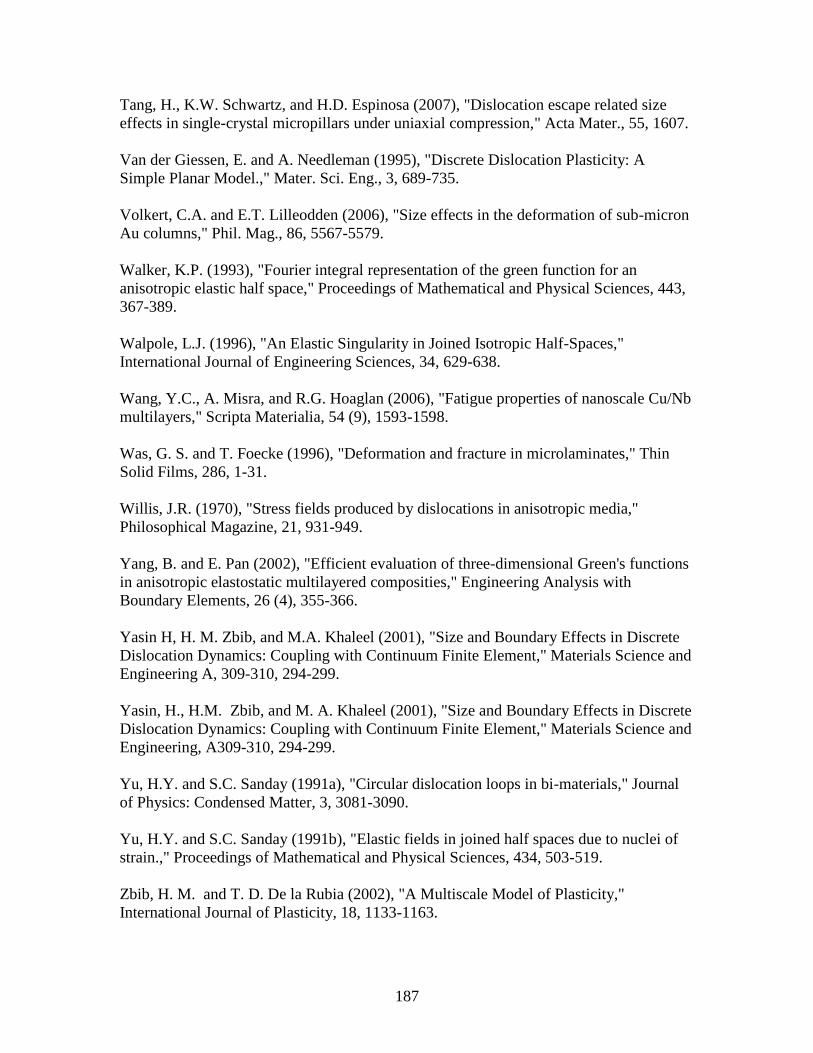
187

Tang, H., K.W. Schwartz, and H.D. Espinosa (2007), "Dislocation escape related size

effects in single-crystal micropillars under uniaxial compression," Acta Mater., 55, 1607.

Van der Giessen, E. and A. Needleman (1995), "Discrete Dislocation Plasticity: A

Simple Planar Model.," Mater. Sci. Eng., 3, 689-735.

Volkert, C.A. and E.T. Lilleodden (2006), "Size effects in the deformation of sub-micron

Au columns," Phil. Mag., 86, 5567-5579.

Walker, K.P. (1993), "Fourier integral representation of the green function for an

anisotropic elastic half space," Proceedings of Mathematical and Physical Sciences, 443,

367-389.

Walpole, L.J. (1996), "An Elastic Singularity in Joined Isotropic Half-Spaces,"

International Journal of Engineering Sciences, 34, 629-638.

Wang, Y.C., A. Misra, and R.G. Hoaglan (2006), "Fatigue properties of nanoscale Cu/Nb

multilayers," Scripta Materialia, 54 (9), 1593-1598.

Was, G. S. and T. Foecke (1996), "Deformation and fracture in microlaminates," Thin

Solid Films, 286, 1-31.

Willis, J.R. (1970), "Stress fields produced by dislocations in anisotropic media,"

Philosophical Magazine, 21, 931-949.

Yang, B. and E. Pan (2002), "Efficient evaluation of three-dimensional Green's functions

in anisotropic elastostatic multilayered composities," Engineering Analysis with

Boundary Elements, 26 (4), 355-366.

Yasin H, H. M. Zbib, and M.A. Khaleel (2001), "Size and Boundary Effects in Discrete

Dislocation Dynamics: Coupling with Continuum Finite Element," Materials Science and

Engineering A, 309-310, 294-299.

Yasin, H., H.M. Zbib, and M. A. Khaleel (2001), "Size and Boundary Effects in Discrete

Dislocation Dynamics: Coupling with Continuum Finite Element," Materials Science and

Engineering, A309-310, 294-299.

Yu, H.Y. and S.C. Sanday (1991a), "Circular dislocation loops in bi-materials," Journal

of Physics: Condensed Matter, 3, 3081-3090.

Yu, H.Y. and S.C. Sanday (1991b), "Elastic fields in joined half spaces due to nuclei of

strain.," Proceedings of Mathematical and Physical Sciences, 434, 503-519.

Zbib, H. M. and T. D. De la Rubia (2002), "A Multiscale Model of Plasticity,"

International Journal of Plasticity, 18, 1133-1163.

188

Zbib, H. M. and E. C. Aifantis (1989a), "A Gradient-Dependent Flow Theory of

Plasticity: Application to Metal and Soil Instabilities," ASME J. Appl. Mech. Rev, 42

(No. 11, Part 2), 295-304.

Zbib, H. M. and E.C. Aifantis (1989b), "On the localization and post-localization of

plastic deformation I," Res Mechanica, 23, 261-277.

Zbib, H. M. and E.C. Aifantis (1989c), "On the localization and post-localization of

plastic deformation II," Res Mechanica, 23, 279-292.

Zbib, H. M. and E.C. Aifantis (1989d), "On the localization and post-localization of

plastic deformation III," Res Mechanica, 23, 293-305.

Zbib, H. M., T. D. De la Rubia, and V. V. Bulatov (2002a), "A Multiscale Model of

Plasticity based on Discrete Dislocation Dynamics," ASME-Journal of Engineering

Materials and Technology, 124, 78-87.

Zbib, H. M., T. D. De la Rubia, M. Rhee, and J. P. Hirth (2000), "3D Dislocation

Dynamics: Sress-Strain behavior and Hardening Mechanisms in FCC and BCC Metals,"

Journal of Nuclear Materials, 276, 154-165.

Zbib, H. M., M Rhee, and J. P. Hirth (1996a), "3D simulation of curved dislocations:

Discretization and long range interactions," in Advances in Engineering Plasticity and its

Applications, T. Abe and T. Tsuta, Eds. New York: Pergamon.

Zbib, H.M. and T. Diaz de la Rubia (2002), "A Multiscale Model of Plasticity," Int. J.

Plasticity, 18 (9), 1133-1163.

Zbib, H.M., T. Diaz de la Rubia, and V. A. Bulatov (2002b), "A Multiscale Model of

Plasticity Based on Discrete Dislocation Dynamics," ASME J. Enger. Mater, Tech., 124,

78-87.

Zbib, H.M., M. Rhee, and J.P. Hirth (1998), "On Plastic Deformation and the Dynamcis

of 3D Dislocations," International Journal of Mechanical Science, 40, 113-127.

Zbib, H.M., M. Rhee, and J.P. Hirth (1996b), "3D Simulation of Curved Dislocations:

Discretization and Long Range Interactions," Advances in Engineering Plasticity and its

Applications, eds. T. Abe and T. Tsuta. Pergamon, NY, 15-20.

Zhang, G. P., C. A. Volkert, R. Schwaiger, E. Arzt, and O. Kraft (2005), "Damage

behavior of 200-nm thin copper films under cyclic loading," Journal of Materials

research, 20 (1), 201-207.