COMPUTATIONAL MODELING OF WORD LEARNING: THE ROLE OF
COGNITIVE PROCESSES
by
Aida Nematzadeh
A thesis submitted in conformity with the requirementsfor the degree of Doctor of Philosophy
Graduate Department of Computer ScienceUniversity of Toronto
c© Copyright 2015 by Aida Nematzadeh
Abstract
Computational Modeling of Word Learning: The Role of Cognitive Processes
Aida Nematzadeh
Doctor of Philosophy
Graduate Department of Computer Science
University of Toronto
2015
Young children, with no prior knowledge, learn word meanings from a highly noisy and
ambiguous input. Moreover, child word learning depends on other cognitive processes such
as memory, attention, and categorization. Much research has focused on investigating how
children acquire word meanings. A promising approach to study word learning (or any aspect
of language acquisition) is computational modeling since it enables a precise implementation
of psycholinguistic theories. In this thesis, I investigate the mechanisms involved in word
learning through developing a computational model. Previous computational models often
do not examine vocabulary development in the context of other cognitive processes. I argue
that, to provide a better account of child behavior, we need to consider these processes when
modeling word learning. To demonstrate this, I study three phenomena observed in child word
learning.
First, I show that individual differences in word learning can be captured through modeling
the variations in attentional development of learners. Understanding these individual differ-
ences is important since although most children are successful word learners, some exhibit
substantial delay in word learning and may never reach the normal level of language efficacy.
Second, I have studied certain phenomena (such as the spacing effect) where the difficulty of
learning conditions results in better retention of word meanings. The results suggest that these
phenomena can be captured through the interaction of attentional and forgetting mechanisms
in the model. Finally, I have investigated how children, as they gradually learn word meanings,
ii
acquire the semantic relations among them. I propose an algorithm that uses the similarity of
words in semantic categories and the context of words, to grow a semantic network. The result-
ing semantic network exhibits the structure and connectivity of adult semantic knowledge. The
results in these three areas confirm the effectiveness of computational modeling of cognitive
processes in replicating behavioral data in word learning.
iii
Acknowledgements
It took me a very long time to write this acknowledgment section; every time I started to
write, my mind would wander to the last seven years and to how my journey of graduate
studies started and ended. (Also, a friend of mine keeps telling me that you learn a lot about
someone from reading the acknowledgment of their thesis!) During this time, I have grown
both academically and personally, and I feel very lucky to have enjoyed it as well. Of course,
many wonderful people played a role. This is an attempt to thank them.
When I moved to Toronto in 2008, I was very excited to do research without knowing
much about what “research” is. Suzanne Stevenson, my advisor, patiently worked with me as
an MSc and then a PhD student. Suzanne taught me to be critical of my work, to explain it
clearly, and to be honest about its strengths and shortcomings. During these years, the clarity
of her thought has helped me gain a better understanding of my research. I have been inspired
by Suzanne’s high standards, academic integrity, and her passion for education. For these and
so many other reasons, including her friendship, I am grateful to Suzanne. I also wish to thank
Sven Dickinson, who, although was not directly involved in my research, gave me excellent
advice on hard decisions, always with a positive perspective. His exuberant personality has
also been a mood lifter even after the briefest of conversations.
I was fortunate to have Afsaneh Fazly as my unofficial co-advisor, not to mention mentor
and friend. I enjoyed our close collaboration from the beginning and have learned a lot from
our discussions, some of which had nothing to do with research. I admire Afsaneh’s approach
to research and collaboration: she dives into problems and never withholds her time and en-
ergy. Afsaneh and Reza Azimi also made my transition much easier, especially during my first
months in Toronto. They invited me to their place soon after I arrived in Toronto when I was
missing a homemade meal terribly. Thanks Afsaneh and Reza!
I also wish to thank the other members of my advisory committee, Graeme Hirst and
Richard Zemel. Graeme’s insightful questions and detailed comments on my research, writ-
ings, and presentations have helped me become a better researcher. He guided me through
iv
various applications, and provided useful feedback on how to teach a class. His dedication to
the Computational Linguistics group sets a great example of what it means to be a devoted aca-
demic. I have benefited from Rich’s abstract look at problems and his deep understanding of
modeling. His questions helped me be more concise yet at the same time see the forest through
the trees. I am likewise thankful to Mike Mozer, my external examiner, for his detailed study of
my thesis. His questions, comments, and suggestions provided me with much to contemplate.
Also, thank you for taking time to come to Toronto for my defense! I also wish to thank Sanja
Fidler, my internal examiner, for her time and valuable feedback on my thesis.
During my PhD, I completed two fruitful research visits that helped me become a better
scholar. I wish to thank Marius Pasca, my mentor at Google Research, and Srini Narayanan
and Behrang Mohit, my mentors at International Computer Science Institute at Berkeley. I am
also thankful to Thomas Griffiths for having me as a visiting student in his lab, and for his time
and feedback on my research.
During these years, I have had the opportunity to interact with many great colleagues in the
Department of Computer Science. I would like to thank the members of SuzGrp, Libby Barak,
Barend Beekhuizen, Paul Cook, Erin Grant, and Chris Parisien for discussions, motivations,
our reading group meetings, and for providing feedback on my work in progress. Chris and
Paul patiently answered my questions when I started my MSc degree. It has been a lot of
fun to work with Erin. Libby has been a good friend and an awesome conference buddy. I
have enjoyed her forthright and insightful style, as well as our many personal and academic
chats. Moreover, I am grateful to all the past and present members of the Computational
Linguistics group for valuable comments and suggestions on my work and talks and also for
being easygoing, helpful, and fun. Thanks especially to Varada Kolhatkar, a good friend and
colleague, for our long discussions on research, especially during the last year, and for our
random chats. I also would like to thank Inmar Givoni for her mentorship and Abdel-rahman
Mohamed for his encouragement.
Our department has the most helpful and friendliest staff who have saved me many times. In
v
particular, I would like to thank Luna Boodram, Linda Chow, Lisa DeCaro, Marina Haloulos,
Vinita Krishnan, Relu Patrascu, Joseph Raghubar, and Julie Weedmark. I am also thankful to
the staff of the Office of the Dean, Faculty of Arts and Science; especially, thanks to Mary-
Catherine Hayward, and all of Suzanne’s assistants during these years.
Graduate school would not have been as memorable and joyful without the wonderful and
smart people that I have been lucky to be surrounded by. I am thankful to Siavosh Benab-
bas, Hanieh Bastani, Aditya Bhargava, Julian Brooke, Orion Buske, Eric Corlett, Niusha De-
rakhshan, Golnaz Elahi, Maryam Fazel, Yuval Filmus, Katie Fraser, Jairan Gahan, Golnaz
Ghasemiesfeh, Michael Guerzhoy, Olga Irzak, Siavash Kazemian, Saman Khoshbakht, Xuan
Le, Meghana Marathe, Nona Naderi, Mohammad Norouzi, Mahnaz Rabbani, Ilya Sutskever,
Giovanna Thron, Joel Oren, and Tong Wang for being great company, and for conversations,
lunch/tea/coffee breaks, dinners, parties, and board games. Moreover, thanks to Jane White
who gave me a sense of home when I lived in Berkeley, inspiring me with her energetic char-
acter. I would also like to thank all friends during my research visits, especially Wiebke and
Erik Rodner.
I also wish to thank all my friends from high school and university, now living all around
the world, who I got to hang out with at random times in different cities. Thanks in particular to
Morteza Ansarinia, Fatemeh Hamzavi, Sara Hadjimoradlou, Anna Jafarpour, Ida Karimfazli,
Mina Mani, and Parisa Mirshams for their friendship and encouragement. Moreover, I am
thankful to the teachers who – although indirectly – played an important role in this journey;
in particular, thanks to Bahman Pourvatan and Hossein Pedram, and my high school math
teachers, Ms. Navid and Ms. Salehi. I am also thankful to Kerry Kim for his drawing classes
that reminded me that we learn from failure and that we should focus on our strengths but work
on our weaknesses.
I wish to thank all my wonderful friends who, throughout my life, and particularly during
graduate school, supported me, helped me find purpose and keep my sanity. Milad Eftekhar
is patient, a great listener, and a wonderful gym buddy/coach. Alireza Sahraei is adventurous
vi
and bold and has inspired me to try new things. Lalla Mouatadid is cheerful, determined, and
a great companion. Jackie Chi Kit Cheung has been a great friend and colleague since I moved
to Toronto. Thanks Jackie for our food and city explorations, for patiently introducing me to
new board games, and for feedback on my work. Also, thanks for keeping the Computational
Linguistics group more active. Reihaneh Rabbany, is affable, generous, understanding, and
was a great study buddy. Bahar Aameri and Nezam Bozorgzadeh have been supportive and
sympathetic for so many years. I have known Bahar since I was fourteen; she is as compas-
sionate as she is rational and reliable, and has been my confidante. Nezam is warm-hearted
with a good taste in music and food, and is always willing to lend a hand. Also, thanks to
Sebastian the cat, for reminding me to take it easy when things do not matter.
Finally, I am forever grateful to my family. My parents have always been very loving and
supportive of my decisions even when they found them unorthodox. I am grateful for the
sacrifices they have made to enable me to follow my own path. My mom, Soheila Hejazi,
has always inspired me by her curiosity to learn and by her persistence. My dad, Feridoon
Nematzadeh, taught me that character is more important than intellect. My sister, Azadeh
Nematzadeh, is one of the most generous, courageous, and resilient people that I know. I
have been very lucky to have her to look up to when I was younger, and to have always had
her energy and encouragement. Lastly, I wish to thank Amin Tootoonchian. Being around his
spirited and upbeat character has been amazing; I have admired his positive approach to life and
people, which I hope has rubbed off on me. He proofread most of what I wrote throughout my
PhD, and has listened to many of my ideas and work in progress. I have enjoyed his perception
and intelligence when having serious conversations as well as when playing fun games. Thank
you, Amin, for making everything in life more gratifying.
vii
Contents
1 Introduction 1
2 Word Learning in Children and Computational Models 7
2.1 The Complexity of Learning Word Meanings . . . . . . . . . . . . . . . . . . 7
2.2 Psycholinguistic Theories of Word Learning . . . . . . . . . . . . . . . . . . . 9
2.2.1 Patterns Observed in Child Word Learning . . . . . . . . . . . . . . . 10
2.2.2 Word Leaning: Constraints and Mechanisms . . . . . . . . . . . . . . 11
2.3 Computational Models of Word Learning . . . . . . . . . . . . . . . . . . . . 14
2.3.1 The Role of Computational Modelling . . . . . . . . . . . . . . . . . . 15
2.3.2 Learning Single Words . . . . . . . . . . . . . . . . . . . . . . . . . . 17
2.3.3 Learning Words from Context . . . . . . . . . . . . . . . . . . . . . . 20
2.3.4 Summary . . . . . . . . . . . . . . . . . . . . . . . . . . . . . . . . . 27
2.4 Modeling Word Learning: Foundations . . . . . . . . . . . . . . . . . . . . . 28
2.4.1 Model Input and Output . . . . . . . . . . . . . . . . . . . . . . . . . 29
2.4.2 Learning Algorithm . . . . . . . . . . . . . . . . . . . . . . . . . . . 29
3 Individual Differences in Word Learning 32
3.1 Background on Late Talking . . . . . . . . . . . . . . . . . . . . . . . . . . . 32
3.2 Modeling Changes in Attention over Time . . . . . . . . . . . . . . . . . . . . 34
3.3 Experiments on Attentional Development . . . . . . . . . . . . . . . . . . . . 37
3.3.1 Experimental Setup . . . . . . . . . . . . . . . . . . . . . . . . . . . . 37
viii
3.3.2 Experiment 1: Patterns of Learning . . . . . . . . . . . . . . . . . . . 39
3.3.3 Experiment 2: Novel Word Learning . . . . . . . . . . . . . . . . . . . 41
3.3.4 Experiment 3: Semantic Connectivity . . . . . . . . . . . . . . . . . . 44
3.3.5 Summary . . . . . . . . . . . . . . . . . . . . . . . . . . . . . . . . . 46
3.4 Learning Semantic Categories of Words . . . . . . . . . . . . . . . . . . . . . 48
3.5 Experiments on Categorization . . . . . . . . . . . . . . . . . . . . . . . . . . 50
3.5.1 Experimental Setup . . . . . . . . . . . . . . . . . . . . . . . . . . . . 51
3.5.2 Experiment 1: Analysis of the Learned Clusters . . . . . . . . . . . . . 53
3.5.3 Experiment 2: Incorporating Categories in Word Learning . . . . . . . 54
3.5.4 Experiment 3: Category Knowledge in Novel Word Learning . . . . . . 56
3.5.5 Summary . . . . . . . . . . . . . . . . . . . . . . . . . . . . . . . . . 58
3.6 Constructing a Learner’s Semantic Network . . . . . . . . . . . . . . . . . . . 59
3.7 Experiments on Semantic Networks . . . . . . . . . . . . . . . . . . . . . . . 62
3.7.1 Evaluating the Networks’ Structural Properties . . . . . . . . . . . . . 62
3.7.2 Experimental Setup . . . . . . . . . . . . . . . . . . . . . . . . . . . . 65
3.7.3 Experimental Results . . . . . . . . . . . . . . . . . . . . . . . . . . . 65
3.7.4 Summary . . . . . . . . . . . . . . . . . . . . . . . . . . . . . . . . . 72
3.8 Conclusions . . . . . . . . . . . . . . . . . . . . . . . . . . . . . . . . . . . . 73
4 Memory, Attention, and Word Learning 74
4.1 Related Work . . . . . . . . . . . . . . . . . . . . . . . . . . . . . . . . . . . 74
4.2 Modeling Attention and Forgetting in Word Learning . . . . . . . . . . . . . . 76
4.2.1 Adding Attention to Novelty to the Model . . . . . . . . . . . . . . . . 77
4.2.2 Adding a Forgetting Mechanism to the Model . . . . . . . . . . . . . . 78
4.3 Experiments on Spacing Effect . . . . . . . . . . . . . . . . . . . . . . . . . . 79
4.3.1 Experiment 1: Word Learning over Time . . . . . . . . . . . . . . . . 80
4.3.2 Experiment 2: The Spacing Effect in Novel Word Learning . . . . . . . 81
4.3.3 Experiment 3: The Role of Forgetting and Attention . . . . . . . . . . 85
ix
4.3.4 Experiment 4: The “Spacing Crossover Interaction” . . . . . . . . . . 87
4.3.5 Summary . . . . . . . . . . . . . . . . . . . . . . . . . . . . . . . . . 88
4.4 Desirable Difficulties in Word Learning . . . . . . . . . . . . . . . . . . . . . 90
4.5 Experiments on Desirable Difficulties . . . . . . . . . . . . . . . . . . . . . . 93
4.5.1 Methodology . . . . . . . . . . . . . . . . . . . . . . . . . . . . . . . 93
4.5.2 Experiment 1: The Input of V&S . . . . . . . . . . . . . . . . . . . . 95
4.5.3 Experiment 2: Randomly Generated Input . . . . . . . . . . . . . . . . 97
4.5.4 Summary . . . . . . . . . . . . . . . . . . . . . . . . . . . . . . . . . 99
4.6 Conclusions . . . . . . . . . . . . . . . . . . . . . . . . . . . . . . . . . . . . 100
5 Semantic Network Learning 102
5.1 Related Work . . . . . . . . . . . . . . . . . . . . . . . . . . . . . . . . . . . 104
5.2 The Incremental Network Model . . . . . . . . . . . . . . . . . . . . . . . . . 105
5.2.1 Growing a Semantic Network . . . . . . . . . . . . . . . . . . . . . . 105
5.2.2 Semantic Clustering of Word Tokens . . . . . . . . . . . . . . . . . . 107
5.3 Evaluation . . . . . . . . . . . . . . . . . . . . . . . . . . . . . . . . . . . . . 110
5.3.1 Evaluating Semantic Connectivity . . . . . . . . . . . . . . . . . . . . 110
5.3.2 Evaluating the Structure of the Network . . . . . . . . . . . . . . . . . 112
5.4 Experimental Setup . . . . . . . . . . . . . . . . . . . . . . . . . . . . . . . . 112
5.4.1 Input Representation . . . . . . . . . . . . . . . . . . . . . . . . . . . 112
5.4.2 Methods . . . . . . . . . . . . . . . . . . . . . . . . . . . . . . . . . 113
5.4.3 Experimental Parameters . . . . . . . . . . . . . . . . . . . . . . . . . 115
5.5 Experimental Results . . . . . . . . . . . . . . . . . . . . . . . . . . . . . . . 117
5.6 Conclusions . . . . . . . . . . . . . . . . . . . . . . . . . . . . . . . . . . . . 118
6 Conclusions 120
6.1 Summary of Contributions . . . . . . . . . . . . . . . . . . . . . . . . . . . . 120
6.2 Future Directions . . . . . . . . . . . . . . . . . . . . . . . . . . . . . . . . . 122
x
6.2.1 Short-term Extensions . . . . . . . . . . . . . . . . . . . . . . . . . . 122
6.2.2 Long-term Goals . . . . . . . . . . . . . . . . . . . . . . . . . . . . . 123
6.3 Concluding Remarks . . . . . . . . . . . . . . . . . . . . . . . . . . . . . . . 125
Bibliography 126
xi
List of Figures
3.1 Sample sensory-motor features and their ratings for “box”. . . . . . . . . . . . 38
3.2 Proportion of noun/verb word types learned. . . . . . . . . . . . . . . . . . . . 40
3.3 Average Comp probabilities of learners over time. . . . . . . . . . . . . . . . . 42
3.4 Average Prod probabilities of learners over time. . . . . . . . . . . . . . . . . 44
3.5 Semantic connectivity scores of learners over time. . . . . . . . . . . . . . . . 46
3.6 Sample gold-standard meaning features and their scores for “apple”. . . . . . . 52
3.7 Change in the average Acq score of all nouns over time. . . . . . . . . . . . . . 56
3.8 Changes in the novel word learning over time. . . . . . . . . . . . . . . . . . . 58
3.9 The gold-standard and ND networks. . . . . . . . . . . . . . . . . . . . . . . . 67
3.10 The degree distributions of Net-GS and Net-ND. . . . . . . . . . . . . . . . . 68
3.11 The network of LT with all words connected by learned meanings (Net-LT). . . 69
3.12 The degree distributions of Net-LT. . . . . . . . . . . . . . . . . . . . . . . . . 69
4.1 Average acq score of the words over time, for our model and FAS’s model. . . 81
4.2 Example stimuli taken from Vlach et al. (2008) . . . . . . . . . . . . . . . . . 82
4.3 Spacing and retention intervals . . . . . . . . . . . . . . . . . . . . . . . . . . 82
4.4 Average acq score of the novel words over spacing intervals. . . . . . . . . . . 84
4.5 Average acq score for the model with attention to novelty but without forgetting. 86
4.6 Average acq score for the model with forgetting but without attention to novelty. 87
4.7 Average acq score of the novel words over spacing intervals . . . . . . . . . . 89
4.8 Example stimuli from 2× 2 condition taken from V&S. . . . . . . . . . . . . . 91
xii
4.9 The results of V&S’s experiment. . . . . . . . . . . . . . . . . . . . . . . . . 92
4.10 Average acq score of words with similar conditions as the V&S experiments. . 96
4.11 Average acq score of words averaged over 20 sets of stimuli. . . . . . . . . . . 98
5.1 Semantic clustering versus a semantic network. . . . . . . . . . . . . . . . . . 107
5.2 Finding the rank of the first five “gold-standard” associates for the word “panda”.112
xiii
Chapter 1
Introduction
Children start to learn the meaning of words very early on in their development: Most chil-
dren produce simple words by the age of one. Word learning is significant in child language
development since comprehending the meaning of single words is the first step in understand-
ing larger linguistic units such as phrases and sentences. Moreover, this knowledge of word
meanings helps a child understand the relations among the words in a sentence; thus it facili-
tates the acquisition of syntax, which is necessary for language comprehension and production.
A child’s knowledge of words includes aspects beyond word meanings (such as phonology);
however, in this thesis, word learning refers to the process of learning word meanings.
Child word learning happens simultaneously with and depends on the development of other
cognitive processes such as memory, attention, and categorization: Human memory organizes
the knowledge of word meanings in an efficiently accessible way (e.g., Collins and Loftus,
1975). Moreover, forgetting (a side effect of memory) impacts children’s retention of word
meanings (e.g., Vlach et al., 2008). Previous research also shows that the ability to attend
to the relevant aspects of a word-learning environment is crucial in learning word meanings
(e.g., Mundy et al., 2007). Moreover, forming categories of word meanings provides abstract
knowledge about properties relevant to each category; this additional knowledge is beneficial
to subsequent word learning (e.g., Jones et al., 1991).
1
CHAPTER 1. INTRODUCTION 2
Much research has focused on shedding light on how children learn the meaning of words.
Researchers have different views about what aspects of this process (and language acquisi-
tion in general) are innate: the linguistic knowledge, the learning mechanisms, or both. The
work in this thesis is in line with the view that language acquisition is a result of applying
domain-general cognitive abilities (such as memory and attentional skills) to the linguistic in-
put with no need for a “special cognitive system” (e.g., Saffran et al., 1999; Tomasello, 2005).
In contrast, others argue that children are born with innate linguistic knowledge or a language-
specific module, and because of this domain-specific knowledge or cognitive system, they can
acquire a language. A common justification of such theories is that all languages have many
commonalities that must be innate (Chomsky, 1993; Hoff, 2009).
The two sides of this issue parallel the ongoing nature-nurture debate, i.e., whether lan-
guage is an innate endowment that only humans are equipped with, or a skill that children
acquire from their environment (Hoff, 2009). The nativist view or nativism claims that the
human mind is wired with a specific structure for learning languages (Pinker, 1994; Chomsky,
1993). Nativists often compare the acquisition of language to how the body grows and ma-
tures, and they argue that since it is “rapid, effortless, and untutored” (Hoff, 2009), it is more
similar to maturation than learning (Chomsky, 1993). The extreme opposite view of nativism,
the empiricist view, asserts that children have no pre-existing knowledge of language, and their
mind is like a “blank slate”. In this view, language is acquired only through experience. In this
thesis, I assume that linguistic knowledge is not innate, and children learn their language by
processing the input they receive using general cognitive (learning) mechanisms.
Several methodologies are available for studying word learning, such as controlled exper-
iments in a laboratory and observational studies in a child’s natural environment. I use com-
putational modelling to study the mechanisms underlying word learning, because it provides
a precise and testable implementation of psycholinguistic hypotheses. Computational model-
ing also enables full control over experimental settings, making it possible to examine a vast
number of conditions difficult to achieve with human subjects. Moreover, the predictions of a
CHAPTER 1. INTRODUCTION 3
computational model – one that has been throughly evaluated against behavioral data – can in
turn be validated with human experiments.
The focus of this thesis is to investigate how children acquire word meanings through com-
putational modeling of word learning and other cognitive processes. The main hypothesis of
this thesis is that we can account for child behavior in word learning better when a model in-
tegrates it with other cognitive mechanisms such as memory and attention. I investigate this
hypothesis by studying three important phenomena observed in child vocabulary development:
• Individual differences in word learning. Even though most children are successful word
learners, some children, known as late talkers, show a marked delay in vocabulary ac-
quisition and are at risk for specific language impairment. Much research has focused on
identifying factors contributing to this phenomenon. We use our computational model
of word learning to further shed light on these factors. In particular, we show that varia-
tions in the attentional abilities of the computational learner can be used to model various
identified differences in late talkers compared to normally-developing children: delayed
and slower vocabulary growth, greater difficulty in novel word learning, and decreased
semantic connectedness among learned words.
• The role of forgetting in word learning. Retention of words depends on the circumstances
in which the words are learned: A well-known phenomenon – the spacing effect – is the
observation that distributing (as opposed to cramming) learning events over a period of
time significantly improves long-term learning. Moreover, certain difficulties of a word-
learning situation can promote long-term learning, and thus are referred to as desirable
difficulties. We use our computational model, which includes mechanisms to simulate
attention and forgetting, to examine the possible explanatory factors of these observed
patterns in cross-situational word learning. Our model accounts for experimental results
on children as well as several patterns observed in adults. Our findings also emphasize
the role of computational modeling in understanding empirical results.
CHAPTER 1. INTRODUCTION 4
• Learning semantic relations among words. Children simultaneously learn word mean-
ings and the semantic relations among words, and also efficiently organize this informa-
tion. A presumed outcome of this development is the formation of a semantic network
– a graph of words as nodes and semantic relations as edges – that reflects this semantic
knowledge. We present an algorithm for simultaneously learning word meanings and
gradually growing a semantic network. We demonstrate that the evolving semantic con-
nections among words in addition to their context are necessary in forming a semantic
network that resembles an adult’s semantic knowledge.
In each chapter of this thesis, I demonstrate that these phenomena can only be explained
when word learning is modelled in the context of other cognitive processes. Moreover, the
modeling in each chapter helps shed light on the mechanisms involved in vocabulary develop-
ment. Understanding this process is a significant research problem for a variety of reasons: It
can facilitate the identification, prevention, or treatment of language deficits. It can also result
in educational methods that improve students’ learning. More generally, understanding the
mechanisms involved in language learning can help us build more powerful natural language
processing (NLP) systems, because most NLP applications need to address the same challenges
that people face in language acquisition.
This thesis is organized as follows: Chapter 2 discusses the relevant psycholinguistic (Sec-
tion 2.1 and Section 2.2) and computational modeling (Section 2.3) background on word learn-
ing. Section 2.4 provides a detailed explanation of the model of Fazly et al. (2010b), which is
the basis for modeling proposed in this thesis.
Chapter 3 focuses on modeling individual differences in word learning. In Section 3.2, I
explain how attentional development is simulated in the context of the proposed computational
model of word learning. Section 3.3 discusses our experimental results in replicating behav-
ioral data on late-talking and normally-developing children. Section 3.4 explains the extension
to the model for semantic category formation, which is used to further examine the differ-
ences observed in late-talking and normally developing children. Section 3.5 provides our
CHAPTER 1. INTRODUCTION 5
experimental results on the role of categorization in individual differences in word learning.
In Section 3.6 and Section 3.7, we examine the structural differences in children’s vocabulary.
This chapter consists of the work published in the following papers:
• A computational study of late talking in word-meaning acquisition.
A. Nematzadeh, A. Fazly, and S. Stevenson.
In Proceedings of the 33th Annual Conference of the Cognitive Science Society, pages
705-710, 2011.
• Interaction of word learning and semantic category formation in late talking
A. Nematzadeh, A. Fazly, and S. Stevenson.
In Proceedings of the 34th Annual Conference of the Cognitive Science Society, pages
2085-2090, 2012.
• Structural differences in the semantic networks of simulated word learners.
A. Nematzadeh, A. Fazly, and S. Stevenson.
In Proceedings of the 36th Annual Conference of the Cognitive Science Society, pages
1072-1077, 2014.
Chapter 4 examines the role of memory and attention in word learning. In Section 4.2,
I explain how attentional and forgetting mechanisms are modeled within the word learning
framework. Section 4.3 discusses our experiments where we replicate several observed pat-
terns on the spacing effect in child and adults. Section 4.4 and Section 4.5 focus on another
phenomenon, desirable difficulty in word learning, that further demonstrates the role of mem-
ory and attention in word learning. The work presented in this chapter has been published in
the papers listed below:
• A computational model of memory, attention, and word learning.
A. Nematzadeh, A. Fazly, and S. Stevenson.
In Proceedings of the 3rd Workshop on Cognitive Modeling and Computational Linguis-
tics (CMCL 2012), pages 80-89. Association for Computational Linguistics, 2012.
CHAPTER 1. INTRODUCTION 6
• Desirable difficulty in learning: A computational investigation.
A. Nematzadeh, A. Fazly, and S. Stevenson.
In Proceedings of the 35th Annual Conference of the Cognitive Science Society, pages
1073-1078, 2013.
The focus of Chapter 5 is learning a semantic network and word meanings simultaneously.
In Section 5.1, I explain the related work. Section 5.2 provides a detailed account of our
proposed model. In Section 5.3, I discuss how we evaluate the semantic connectivity and
structure of semantic networks. Section 5.4 and Section 5.5 discuss our experimental setup
and results on different methods for growing semantic networks. The work in this chapter is
published in:
• A cognitive model of semantic network learning.
A. Nematzadeh, A. Fazly, and S. Stevenson.
In Proceedings of the 2014 Conference on Empirical Methods in Natural Language Pro-
cessing (EMNLP), pages 244254. ACL, 2014.
Chapter 6 is the concluding chapter: Section 6.1 summarizes the contributions of this the-
sis. I provide some possible directions for future research in Section 6.2, and conclude in
Section 6.3.
Chapter 2
Word Learning in Children and
Computational Models
Previous research attempts to shed light on child semantic acquisition using behavioral exper-
iments and computational modelling. In this chapter, I first explain why word learning is a
challenging problem. I also summarize the key theories on child word learning, including pre-
dominant patterns observed in word learning and mechanisms and constraints involved in it.
Then, I explain the major computational models of word learning, as well as the word learning
framework that the model in thesis is based on.
2.1 The Complexity of Learning Word Meanings
Learning the meaning of words is one of the challenging problems that children face in lan-
guage acquisition. Quine (1960) elaborates the word learning problem by providing an inter-
esting example: A linguist aims to learn the language of a group of untouched people. Imagine
a scenario in which she observes a white rabbit jumping around and hears a native saying
“gavagai”. What is the correct meaning of the word “gavagai”? Probably the most reasonable
answer is “rabbit”. However, there are plenty of possible options. Imagine the native has seen
a coyote chasing the rabbit: “gavagai” might mean danger, white rabbit, jumping, cute, animal,
7
CHAPTER 2. WORD LEARNING IN CHILDREN AND COMPUTATIONAL MODELS 8
It is hungry, coyote, etc. The linguist needs to hear the word “gavagai” in a variety of situations
to be confident about its meaning. Learning the correct meaning of a word by looking at the
non-linguistic context is referred to as the word-to-world mapping problem (Gleitman, 1990).
In a realistic word learning scenario, when a child hears an utterance, she/he also needs to
figure out what aspects of her/his environment is being talked about. For example, imagine a
situation where a father is cooking his daughter a meal, and tells her “You will have your pasta
in your red plate, soon”. The child is surrounded by numerous events that might relate to the
utterance: daddy is cooking, the kitty is playing on the kitchen floor, the water is boiling in
a pot, etc. This problem – the existence of multiple possible meanings for an utterance – is
called the referential uncertainty problem (Gleitman, 1990; Siskind, 1996). Moreover, a child
might misperceive the environment due to a variety of reasons such as mishearing a word or
not observing all aspects of the scene. (In this example, the child might not see the pasta which
is still boiling in the pot, when she hears the sentence.) We refer to this misperception as noise
or the problem of noisy input (Siskind, 1996; Fazly et al., 2010b).
Word learning, however, is more than learning word-to-world mappings. Children hear
utterances that consist of more than just one word. In an analysis of the child-directed speech
gathered from 90-minute interactions with children (age 2;6) by Rowe (2008), the mean length
of the utterances (MLU) children heard was 4.16 tokens. Consequently, children need to break
each utterance into a set of words, a problem which is referred to as word segmentation. More-
over, most languages are full of multiword constructions (e.g., “give a kiss”) that children must
learn (Goldberg, 1995). Learning these constructions is in particular challenging since children
need to first identify them, and then associate them to a meaning which is often abstract and
non-referential (Fazly et al., 2009; Nematzadeh et al., 2013a). These important issues are ac-
tive areas of research; but in this thesis, I focus on other aspects of word learning, in particular,
the role of cognitive processes in word learning.
CHAPTER 2. WORD LEARNING IN CHILDREN AND COMPUTATIONAL MODELS 9
2.2 Psycholinguistic Theories of Word Learning
Despite all the complexities of word learning, most children are very successful word learn-
ers: Two-year old children typically have a productive vocabulary of 300 words (Fenson et al.,
1994), and average six-year old children has learned over 14000 words (Carey, 1978). Much
psycholinguistic research has thus focused on how children learn the meaning of words and
what factors might play a role in word learning. Various theories have been proposed aiming
to explain different aspects of the problem, and also many experimental studies have been per-
formed to examine these theories and provide insight on child and adult word learning. There
are two general methodologies that psycholinguists use in their studies: The first methodology
consists of observational studies, in which child word learning is examined in a naturalistic
environment, and often for a long period of time (e.g., MacWhinney, 2000; Fenson, 2007; Roy
et al., 2009). These studies are important since they provide opportunities for examining the
longitudinal patterns of word learning. Moreover, some of these studies produce datasets that
are widely used in other research projects (e.g., the CHILDES database,1 and the MacArthur-
Bates communicative developmental inventories (CDI)2). On the other hand, these studies are
often time and resource consuming, and due to the privacy concerns of the children under study,
the data can only be gathered in specific time periods.
The second methodology includes experimental studies in a lab setting, in which children
are often brought to the lab where they are usually trained on a specific task in controlled
conditions, and then their learning is tested. These experiments are significant since they make
it possible to study the role and interaction of possible factors involved in word learning, as
well as the mechanisms and constraints underlying it (e.g., Yurovsky and Yu, 2008; Vlach et al.,
2008; Ichinco et al., 2009). Because of the controlled nature of these experiments, however,
they may differ from naturalistic child word learning scenarios.
I first explain some of the observed patterns in early vocabulary development, and then I
1http://childes.psy.cmu.edu/2http://www.sci.sdsu.edu/cdi/cdiwelcome.htm
CHAPTER 2. WORD LEARNING IN CHILDREN AND COMPUTATIONAL MODELS 10
go over the constraints and mechanisms that might play a role in word learning.
2.2.1 Patterns Observed in Child Word Learning
Infants start as slow and inefficient word learners. In the first year of their life, their productive
vocabulary – words that they not only comprehend but also produce – is very limited (less
than 10 words). However, the rate of productive vocabulary acquisition slightly increases after
the first year: 16- and 24-month-old infants typically produce around 40 and 300 words, re-
spectively (Fenson et al., 1994). Some researchers believe that there is a sharp increase in the
rate of acquisition of productive vocabulary around the time that children have a productive
vocabulary of approximately 50 words. This sudden increase in producing words is referred to
as the vocabulary spurt, the vocabulary burst, or the naming explosion (Bloom, 1973; Ganger
and Brent, 2004). However, there is a debate on the true nature of the vocabulary spurt, and
some researchers claim that the increase in the rate of word production is a gradual rather than
a sudden change: Ganger and Brent (2004) found that only 5 out of the 38 children in their
study exhibited the vocabulary spurt. In addition to the vocabulary spurt, it is observed that 2-
to 3-year-old children can learn the mapping between a new word and a new object only from
one encounter (or sometimes a few exposures). This ability to acquire a word from only a few
instances is known as fast mapping (Carey and Bartlett, 1978). Fast mapping and vocabulary
spurt might suggest that word learning gets easier for children as they grow up, thus children
learn words more rapidly in the second year of their lives, a phenomenon which Regier (2005)
calls the ease of learning.
Early vocabulary development in children undergoes changes other than the ease of learn-
ing. Another area that a change is observed is the sensitivity to phonetic differences of words.
Young infants (14-month-old) can learn the meaning of phonetically dissimilar words; how-
ever, they are less successful at learning phonetically similar words such as “bih” and “dih”
(Stager and Werker, 1997). This difficulty resolves in older infants, and 17- and 20-month-old
infants distinguish between such words (Werker et al., 2002). This gradual change to correctly
CHAPTER 2. WORD LEARNING IN CHILDREN AND COMPUTATIONAL MODELS 11
learning phonetically similar words is referred to as honing of linguistic form by Regier (2005).
Moreover, younger children sometimes cannot generalize a learned word (e.g., “kitty”) for a
referent (a Siamese cat) to other instances of the referent’s category (a Bengal cat), i.e., they
cannot generalize a novel object by shape when the color and texture are different. However,
older children learn to correctly generalize new objects by shape, which in turn boosts their
novel word learning abilities (Samuelson and Smith, 1999; Colunga and Smith, 2005). Regier
(2005) refers to this gradual change in learning word meanings as honing of meaning.
2.2.2 Word Leaning: Constraints and Mechanisms
To learn the meaning of words, children need to induce the correct word–referent pairs from a
large pool of possibilities. A group of researchers have argued that children use specific biases
and constraints to reduce the number of possibilities, thus making the learning problem easier
(e.g., Rosch, 1973; Soja et al., 1985; Markman, 1987, 1992). However, there is an ongoing
debate on the role of these constraints in word learning, whether they are specific to word
learning or are domain-general constraints, and on the learnability versus innateness of these
constraints (see Markman, 1992). I will explain some of the proposed constraints on word
learning.
Upon hearing a word and observing an object, a child could map the word to the object
(e.g., chair), but also to the individual parts of the object (e.g., a leg of the chair), its color,
and so on. The whole-object constraint argues that children initially constrain meanings of
novel words to refer to the whole object instead of its parts (Markman and Hutchinson, 1984;
Soja et al., 1985). Moreover, there are different relations between objects that young children
observe, and they often attend more to thematic relations between objects (e.g., dog and bone)
compared to taxonomic relations (e.g., dog and cat). However, when it comes to labeling a
novel word, they pick the taxonomic relations over thematic ones: Markman and Hutchinson
(1984) presented three objects, a dog which was labeled “dax”, a cat, and a bone to children.
Then, the children were asked to pick another “dax” from the other objects. The children
CHAPTER 2. WORD LEARNING IN CHILDREN AND COMPUTATIONAL MODELS 12
preferred the taxonomic relation and picked the cat over the bone. This preference of children
in picking taxonomic relations is called the taxonomic assumption or the taxonomic constraint
(Markman, 1992).
There is another group of constraints that explain how children generalize object names to
new instances of the object’s category, for example, how children learn that the word “dog”
refers to both a poodle and a beagle. The basic-level assumption claims that young children
appear to associate the words to objects from basic-level categories such as dogs rather than
more general categories like animals, or more specific ones such as golden retrievers (Rosch,
1973).3 Moreover, Landau et al. (1988) propose another constraint, the shape bias, which
argues that children tend to extend the object names by shape rather than color, texture, size,
etc. They performed an experiment in which young children were asked to pick the objects
that correspond to recently learned words. The children picked the objects that had the same
shape as the learned objects, rather than the ones with the same size or texture.
Another proposed constraint that might influence word learning is the mutual exclusivity
assumption, which argues that children limit the number of labels (words) for each type of ref-
erent to one (Markman, 1987; Markman and Wachtel, 1988), based on observations in which
young children tend to allow only one label for each referent. For example, if they already
know that the word “dog” refers to dogs, in the presence of a cat and a dog, they would as-
sociate a new word “cat” to the referent cat. The mutual exclusivity assumption reduces the
ambiguity of a word learning scenario by removing the referents that are already associated
with some words from the set of possible referents for novel words. This assumption can also
help explain the fast mapping pattern observed in children (Heibeck and Markman, 1987). On
the other hand, children learn a second label (synonyms) for some words, which is against the
mutual exclusivity assumption. As a result, there is a debate on the nature and the role of this
3Almost all the members of basic-level categories (e.g., chairs) share a significant number of attributes; asopposed to superordinate categories which are one level more abstract, and only share a few attributes (e.g.,furniture). Moreover, categories that are below the basic-level categories, subordinate categories, share most oftheir attributes with other categories (siblings and parents), for example, kitchen chairs share many attributes withchairs (Rosch et al., 1976).
CHAPTER 2. WORD LEARNING IN CHILDREN AND COMPUTATIONAL MODELS 13
constraint.
Besides the explained constraints, there are a number of more general mechanisms that
might play a role in word learning. The social-pragmatic approach to word learning argues
that word learning is inherently social, and children do not need to rely on any linguistic con-
straints. According to this view, children learn word meanings using their general social-
cognitive skills in an attempt to understand the intentions of the speakers (Tomasello, 1992).
Children use social cues such as speakers’ gaze, gestures, and body language to identify the
speakers’ intentions and establish joint attention, and in turn infer the meaning of words.
Another widely-discussed mechanism is cross-situational learning, which explains how
children learn word meanings from multiple exposures to words in different situations (Pinker,
1989). The main idea of this type of learning is that people are sensitive to the regularities
that repeat in different situations, and use such evidence to identify the commonalities across
situations, and to infer word meanings. As an example, when a child hears sentences such as
“what a cute kitty”, “let’s play with the kitty”, and “be nice to the kitty”, she/he could infer that
the word “kitty” refers to the common reference in all these situations, i.e., a cat. Recent word
learning experiments also confirm that both adults and infants keep track of cross-situational
statistics across individually ambiguous learning trials, and infer the correct word–meaning
mappings even in highly ambiguous conditions (Yu and Smith, 2007; Smith and Yu, 2008;
Yurovsky et al., 2014). This cross-situational statistical learning is significant since it confirms
that people reliably learn the statistical regularities that exist in word learning scenarios.
A few recent studies suggest that people might not keep track of cross-situational statistics
when learning word meanings (Medina et al., 2011; Trueswell et al., 2013). The authors claim
that adults form a single hypothesis about a word’s meaning that they retain across learning
trials. The authors conclude that in these studies word learning is a result of a “one-trial”
procedure as opposed to gradual accumulative learning. However, the results of these stud-
ies are hard to interpret mainly because of the difference between their setup and previous
cross-situational learning experiments. For example, Medina et al. (2011) explicitly asked the
CHAPTER 2. WORD LEARNING IN CHILDREN AND COMPUTATIONAL MODELS 14
participants to make a guess about a word’s meanings (for a discussion see Yurovsky et al.,
2014).
There are two other learning mechanisms that might be responsible for child vocabulary
development. The first one, associative learning, is a general learning mechanism in which
two co-occurring events or objects get associated together (e.g., Colunga and Smith, 2005).
The second mechanism is the hypothesis testing account which argues that children form a set
of hypotheses about word–referent pairings. These hypotheses are evaluated upon receiving
new information, forming a new set of hypotheses, and this process of refining the hypotheses
is repeated until the word–referent pairing is learned (e.g., Siskind, 1996; Xu and Tenenbaum,
2007).
Moreover, some researchers believe that child word learning undergoes a change in the
mechanism, starting with a simple associative mechanism, and changing as a child learns about
the referential nature of words. These researchers argue that some of the observed patterns in
child vocabulary development (such as vocabulary spurt and fast mapping) can be explained
by this change in the learning mechanism (Kamhi, 1986). Note that both hypothesis testing
and associative learning are broad concepts, and researchers often support a variation of these
mechanisms by introducing their specific assumptions. Also, in the context of word learning
the difference between the two learning mechanisms is not well defined (Yu and Smith, 2012);
but it might become clear by examining computational models, which are discussed in the
following sections.
2.3 Computational Models of Word Learning
Computational modelling is a powerful tool to examine psycholinguistic theories of word learn-
ing, to shed light on its underlying mechanisms, and to investigate the interaction of different
factors that might be involved in word learning. The first subsection discusses the role of com-
putational modelling in more detail. Several word learning models have been proposed, which
CHAPTER 2. WORD LEARNING IN CHILDREN AND COMPUTATIONAL MODELS 15
address different aspects of the problem of learning word meanings, are built with specific
assumptions, and use different input and learning algorithms. In the rest of this section, I dis-
cuss some of these models that are selected to be representative of the above-mentioned word
learning theories. The models are explained in two subsections: In the subsection “Learning
Single Words”, the models discussed restrict the problem to learning meanings for a single
word, without considering the sentential context of the word. Given the word–meaning map-
pings, these models usually learn about some aspects of word learning (e.g., shape bias) and/or
produce some observed patterns of word learning (e.g., the vocabulary spurt). In contrast, in
the second subsection “Learning Words in Context”, the models that are explained address the
problem of learning meanings for words that occur with other words in a context of a sentence.
This problem is more complicated than learning single words, because there are potentially
many-to-many mappings between words in context and the meanings, from which only some
mappings are correct. The models need to learn the correct mappings, that is, which words and
meanings are associated together (the mapping problem). Finally, I will conclude the section
with summarizing the drawbacks and advantages of the models, and discussing what is missing
from current models.
2.3.1 The Role of Computational Modelling
Computational models have been used as a significant tool to study language acquisition in the
last two decades, and have gained popularity among many researchers. There are plenty of
reasons behind this trend in using computational modelling: First of all, computational models
enforce a level of precision that psycholinguistic and linguistic theories may lack. Because
of their verbal form, these theories are often high-level and abstract, and do not provide the
necessary details. To turn these theories into models, one needs to explicitly define all the
underlying assumptions about the input data and learning mechanisms, as well as the parame-
ters that might play a role in the phenomenon under study. Moreover, by using computational
models researchers would have control over the input data. Thus, they can easily simulate
CHAPTER 2. WORD LEARNING IN CHILDREN AND COMPUTATIONAL MODELS 16
many longitudinal patterns of learning that are costly to examine in real-world settings. Also,
they can analyze the role of input in learning by varying its quantity and quality. In addition
to control over the input, researchers can manipulate the parameters of the model, making it
possible to examine the effect of a change in their value and also to study the interactions of
several parameters. As in the case of input, it might be hard, expensive or impossible to turn
some of these simulations to a lab experiment (Elman, 2006; Poibeau et al., 2013).
Another advantage of computational models is that they sometimes can produce predictions
about a phenomenon by running simulations that have not been performed as a laboratory ex-
periment. However, for these predictions to be reliable, the input to the models should be
similar to what children receive, and the learning mechanisms need to be cognitively plausible.
The term “cognitive plausibility” may refer to different criteria depending on the context. A
model is often considered to be cognitively plausible if it implements an incremental learning
algorithm, and is in line with memory and processing limitations of people (Poibeau et al.,
2013). Note that computational models of language acquisition cannot replace the experimen-
tal and theoretical studies: the predictions of already-verified models need to be examined
in empirical studies. Moreover, these models can provide new directions for expanding the
existing theories.
Many computational models have been developed to provide insight on child vocabulary
development. These models can be categorized into two groups based on the learning mecha-
nism they implement (Yu and Smith, 2012). The first group contains associative models which
attempt to implement the associative learning mechanism. Many early connectionist models
of word learning belong to this category. The second group includes hypothesis testing mod-
els, that are mostly implemented using a Bayesian modeling framework. However, some early
rule-based approaches also belong to this group (e.g., Siskind, 1996). As is true of the learning
mechanisms, the distinction between the two groups of models is not always clear, and their
intersection is not necessarily empty. For example, the model of Fazly et al. (2010b) keeps
track of hypotheses about word–referent pairs, similar to hypothesis testing models, but also
CHAPTER 2. WORD LEARNING IN CHILDREN AND COMPUTATIONAL MODELS 17
gathers co-occurrence statistics like associative models.
2.3.2 Learning Single Words
As mentioned earlier, one of the debates on word learning is about whether a change in the
learning mechanism is necessary to explain the changes in children’s word learning around
the age of 2 (e.g., becoming able to learn second labels for words). Regier (2005) proposes
that an associative model that gradually learns to attend to relevant aspects of the world would
exhibit the same pattern of learning as children without a need for a change in the learning
mechanism. Regier (2005) models this with a neural net that learns the association between
word forms and their meanings by using a set of attentional weights that capture the selective
attention to specific dimensions (properties) of word forms and meanings. Both word forms
and meanings are artificially-generated bit vectors with equal number of dimensions, where
half of the dimensions are significant, i.e., a pattern over these dimensions is predicative of
meaning for a word and vice versa. The model is trained under gradient descent in error,
using word forms paired with their correct meaning as training input. The model of Regier
replicates four patterns of learning observed in children: (1) the ease of learning a novel noun,
(2) honing of linguistic form, (3) honing of meaning, and (4) learning second labels for words.
The model produces these patterns because in the course of training, the significant dimensions
gradually receive more attentional weight, which in turn results in a better separation of word
form and meaning vectors in a high-dimensional space. Consequently, there is less chance
that the model activates an incorrect meaning for a word, and vice versa. However, the data
used in these experiments is very small (50 word–meaning pairs). As a result, it is possible
that the model would not exhibit the same learning patterns using a more naturalistic dataset.
Moreover, the dimensionality of data (i.e., number of features used to represent words and
meanings) is chosen arbitrarily, and the features do not correspond to real-world linguistic or
perceptual characteristics of words or meanings.
An interesting aspect of children’s word learning is their ability to generalize novel solids
CHAPTER 2. WORD LEARNING IN CHILDREN AND COMPUTATIONAL MODELS 18
by shape and novel non-solids by material. For example, if children are taught that a novel
wooden rectangular-shaped object is called “dax”, they would generalize the word “dax” to
another object that has the same shape but is made of metal. On the other hand, for a non-solid
object such as play dough (that can easily be formed into different shapes), the material would
be significant rather than the shape: when children learn that a rounded shape play dough is
labeled “teema”, they would also associate a rectangular shape made of the play dough with
“teema”. Note that there are two levels of abstractions involved: (1) Children learn to associate
a word (e.g., “ball”) with certain round objects with different materials and/or colors (e.g., a
rubber ball), and then they generalize this word to a similar novel rounded shape object with
a new material and/or color (e.g., a glass ball). This is the first-order generalization, in which
children generalize the learned words to new instances of the word’s category. (2) The second-
order generalization (over-hypothesis) happens when children know that solidity (non-solidity)
is correlated with shape (material); thus, they expect solid (non-solid) objects to be generalized
by their shape (material) (Kemp et al., 2006).
Colunga and Smith (2005) argue that this higher-level distinction between solids and non-
solids is learnable from correlations existing in children’s early noun categories, using an as-
sociative learning approach. To learn these two levels of abstraction, Colunga and Smith train
a multilayer neural network on an input consisting of 20 word categories paired with their
artificially-generated meaning representations. The meaning of each word category is rep-
resented such that solidity and being shape-based, and also non-solidity and being material-
based, are strongly correlated. Colunga and Smith (2005) perform several simulations with
the model, the results of which confirm their hypothesis that an associative model can form
second-order generalizations about solids and non-solids from the existing correlations in data.
Although the authors attempt to generate a data set that resembles naturalistic child input, the
input generation is still artificial, for example the dimensionality of shape and material vectors,
and their values are chosen arbitrarily. Consequently, the noise and variability of the data may
not match naturalistic child input.
CHAPTER 2. WORD LEARNING IN CHILDREN AND COMPUTATIONAL MODELS 19
One of the challenges children overcome in word learning is figuring out which level of
hierarchical taxonomy a word refers to. For example, upon hearing the word “cat” and observ-
ing a Persian cat licking itself, a child faces a variety of possible interpretations. The word
“cat” could refer to Persian cats, cats, mammals, animals, and so forth. Xu and Tenenbaum
(2007) argue that previously proposed approaches (such as associative learning) are not capa-
ble of learning such distinctions (from only a few examples) without assuming built-in biases
(e.g., basic-level category bias). Instead, they propose a Bayesian model for learning the map-
ping between a novel noun and taxonomic categories, from a few examples. The model of
Xu and Tenenbaum (2007) starts with a tree-structured hypothesis space (of categories) gen-
erated from adult similarity judgments. In the formulation of the model, a bias towards more
distinctive categories is incorporated into the prior probability, and the likelihood encodes the
properties of the exemplars the model receives as input. The model replicates the experimen-
tal patterns observed in both children and adults; however, to produce the observed patterns
in adults, a stronger bias for basic-level categories is incorporated into the prior. The authors
argue that the choice of prior might suggest that the adults have formed a bias for basic-level
categories. Finally, although the model of Xu and Tenenbaum (2007) produces similar pat-
terns to the ones observed in children and adults, it is not discussed how the model might learn
the tree-structured hypothesis space. Moreover, the choice of prior has a significant role in
their results: A variation of their model that only implements the prior (without calculating the
likelihood), produces very similar patterns to the one with the complete Bayesian formulation.
Consequently, the role and importance of the learning mechanism is not clear.
As mentioned earlier, Xu and Tenenbaum (2007) use similarity judgements from adult par-
ticipants to build their hypothesis space for three categories (animals, vehicles, and vegetables).
As a result, a limitation of their work is that it is not possible to easily extend their simulations
to other categories. Abbott et al. (2012) propose a method for automatically generating the hy-
pothesis space used in such Bayesian generalization frameworks. To do so, they use WordNet
(Fellbaum, 1998) to generate the tree-structured hypothesis space for concepts, and ImageNet
CHAPTER 2. WORD LEARNING IN CHILDREN AND COMPUTATIONAL MODELS 20
(Deng et al., 2009) to map images to these concepts. Using this hypothesis space, they repli-
cate the results of Xu and Tenenbaum’s (2007) experiments, and also perform a set of new
experiments on three other categories. Because the results produced by this automatically-
generated hypothesis space and those of a manually-generated hypothesis space are similar;
the automatically-generated hypothesis space can be used in any problem that needs a tree-
structured category organization.
2.3.3 Learning Words from Context
Siskind’s (1996) model is one of the first successful models of learning word meanings from
ambiguous contexts including multiple words and multiple meanings, as in actual word learn-
ing. The model is rule-based and incremental: it learns mappings between words and their
meanings by processing one input pair (an utterance of multiple words and its meaning rep-
resentation) at a time, and applying a set of predefined rules to it. These rules are designed
to first find a set of conceptual symbols (e.g., CAUSE, GO, UP) for each word (e.g.,
“raise”), and then form conceptual expressions out of these symbols (e.g., CAUSE(x, GO(y,
UP))). The predefined rules encode some of the proposed word learning mechanisms and con-
straints, such as cross-situational inference and mutual exclusivity (see Section 2.2). Conse-
quently, the model starts with some built-in word learning biases. The input to this model is
an automatically-generated corpus of utterances (represented as bags of words), each paired
with a set of conceptual expressions that are the hypothesized utterance meanings. The input
generation process makes it possible to produce a large corpus; however, both utterances and
their meaning representations are artificial, and do not conform to the distributional properties
of child input.
Siskind (1996) extends the model to work under noise and homonymy by adding some
rules to detect such cases, and using heuristic functions to disambiguate word senses under
homonymy. Because of this extension, the model needs to add a new sense for a word each
time an inconsistency is detected (i.e., noise or homonomy is present in the data). Note that
CHAPTER 2. WORD LEARNING IN CHILDREN AND COMPUTATIONAL MODELS 21
not all the added senses are necessary and relevant, consequently, a sense-pruning mechanism
is applied to remove the senses that are not used frequently in the input. Furthermore, adding
these senses makes the algorithm very time consuming to the extent that a time limit is ap-
plied to discard an utterance that is taking a lot of time to process. Siskind’s model converges
(i.e., learns a lexicon with 95% accuracy) in several experiments varying different parameters
(vocabulary size, noise rate, homonymy rate, degree of referential uncertainty, and conceptual-
symbol inventory size). The model also replicates two important behavioral patterns observed
in child word learning, i.e., fast-mapping and a sudden ease in learning novel words after learn-
ing a partial lexicon. One important shortcoming of this model is that the learning mechanism
is rule-based, and hence is not robust to the level of noise found in naturalistic learning envi-
ronments. Follow-up models have thus turned to probabilistic learning mechanisms in order to
better handle noise and uncertainty in the input.
Yu and Ballard (2007) argue that children use both cross-situational evidence and social
cues available in their input when mapping words to their referents. Based on this idea, they
build a word learning model that learns from cross-situational regularities of the input, and
also integrates social cues, such as the speaker’s visual attention and prosodic cues in speech.
The model is an adaptation of the translation model of Brown et al. (1993): The speaker’s
utterances are considered as one language which is “translated” to a language consisting of the
possible referents for words in the utterance. The input data consists of pairs of utterances and
meaning representations, which are generated using two videos of mother-infant interactions
taken from the CHILDES database. The utterances are mother’s speech represented as bags
of words. Meaning representations are generated by manually identifying objects presented
in the scene when the corresponding utterance was heard. For each input pair, multiple map-
pings are possible between words and objects, from which only some are correct mappings. To
learn the correct mappings, the model uses the EM algorithm to find parameters that maximize
the likelihood of utterances given their meaning representations. Training with the expecta-
tion maximization (EM) algorithm is a batch process and not incremental, in contrast to how
CHAPTER 2. WORD LEARNING IN CHILDREN AND COMPUTATIONAL MODELS 22
children learn their language. Although the data represents a realistic sample of what a child
learner might perceive, it’s very small (less than 600 utterances). Consequently, it is not clear
whether the model scales to a larger input.
Yu and Ballard (2007) integrate two categories of social cues into their model: (1) One
highlights the relevant (attended) objects in each situation, and is generated by manually spec-
ifying what objects both the mother and the child attended to. (2) The second is prosodic cues
that highlight words that are either used to attract the child’s attention or convey important lin-
guistic information. These social cues are integrated into the model by simply applying some
weight functions to each word or object, to give more weight to the highlighted word or the at-
tended object. The authors train four models: the base model using the statistical information,
the base model integrating attentional cues, the base model integrating prosodic cues, and the
base model integrating both kinds of social cues. They find that the model using both atten-
tional and prosodic cues outperforms the other models. This model, moreover, learns stronger
associations between relevant (correct) word–object pairs, and weaker associations between
irrelevant (incorrect) pairs when compared to other models.
Frank et al. (2009) propose a Bayesian framework for modelling word learning from con-
text using speakers’ communicative intentions. They model the speaker’s intention as a subset
of the objects observed during formation of an utterance. The intuition is that the speaker in-
tends to talk about a subset of objects he observes, and uses some words to express this set
of objects. Given a corpus of situations consisting of such words and objects, the goal of the
model is to find the most probable lexicon. Using Bayes rule, Frank et al. estimate the prior
probability and likelihood of each potential lexicon. In calculating the prior, smaller lexicons
are favored. This choice of prior enforces a conservative learning approach, in which learning
all the existing word–object pairs is not a priority. In calculating the likelihood, the authors
further assume that all intentions (subsets of objects) are equally likely. Thus, the model is
not incorporating a fully elaborated model of speaker’s communicative intentions. The lexi-
con with the maximum a posteriori probability is chosen by applying a stochastic search on
CHAPTER 2. WORD LEARNING IN CHILDREN AND COMPUTATIONAL MODELS 23
the space of possible lexicons. The input data is generated using the same videos of mother–
infant play time that Yu and Ballard (2007) used. The meaning representations are similarly
produced, by manually hand-coding all the objects that were visible to the infant upon hear-
ing each utterance. Although the data is very similar to children’s possible input, the size of
the data set is very small, which makes certain longitudinal patterns (e.g., vocabulary spurt)
impossible to examine.
Frank et al. compare their model with several other models (such as a translation model)
in terms of the accuracy of their learned lexicon as well as their ability to infer the speaker’s
intent (i.e., a subset of observed objects for each utterance). Their model chooses the speaker’s
intentions with the highest posterior probability (given the best lexicon). For the other models,
speaker’s intentions are assumed to be the set of objects corresponding to the words in the ut-
terance. To evaluate the results of each model, they are compared to a gold-standard lexicon,
and a gold-standard set of intended objects. The model of Frank et al. outperforms all the other
models in both tasks of learning a lexicon and inferring the speaker’s intentions, confirming the
importance of modelling speaker’s intentions. Moreover, the model replicates several patterns
observed in child word learning, such as the mutual exclusivity bias and fast mapping. How-
ever, the training of the model is a batch process, which is different from child word learning
that is an incremental process.
Fazly et al. (2010b) propose the first incremental and probabilistic model of word learning
from ambiguous contexts. Their model processes one input pair (an utterance represented as a
bag of words and its scene representation consisting of a set of meaning symbols) at a time: It
calculates an alignment probability for each word–meaning pair by probabilistically aligning
(mapping) the words (in the utterance) to the meaning symbols (in the scene representation)
using the current knowledge of word–meaning pairs. Then, the knowledge of word–meaning
pairs is updated using the new alignment probabilities. For each word, the model learns a
probability distribution, or meaning probability, over all possible meaning symbols, which
represents the model’s current knowledge of that word. This distribution is uniform at the
CHAPTER 2. WORD LEARNING IN CHILDREN AND COMPUTATIONAL MODELS 24
beginning, before any input is processed.
The model of Fazly et al. (2010b) is inspired by the translation model of Brown et al. (1993).
However, as opposed to Yu and Ballard (2007), who simply apply the translation model to their
word learning data, Fazly et al. take a different approach in calculating the formulated prob-
abilities in the model. Brown et al. (1993) use the EM algorithm to maximize the likelihood
function, which is done by batch processing all the data at the same time. In contrast, Fa-
zly et al.’s model updates its current knowledge of word–meaning pairs after processing each
input pair, which is more similar to child word learning, since children receive information
incrementally over time. The utterances in the input are taken from the child-directed portion
of the CHILDES database. The scene representation for each utterance is generated auto-
matically, and is a set of meaning symbols corresponding to all words in the utterance. These
meaning symbols are taken from a gold-standard lexicon in which each word is associated with
its correct meaning. Although the scene representations are automatically generated, the input
resembles naturalistic child input in including noise and referential uncertainty. Also the input
is reasonably large (around 170K input pairs), which makes it possible to examine longitudinal
learning patterns. Fazly et al. perform several simulations, and show that the model learns the
meaning of the words under noise and referential uncertainty. Furthermore, their model repli-
cates several results of fast mapping experiments with children, and can learn homonymous
and synonymous words. The model of Fazly et al. is particularly interesting since without
explicitly building in any biases or constraints, it learns the word meanings from ambiguous
semi-naturalistic child data, and also takes an incremental approach to learning. This model is
used as the basis for the word learning framework proposed in this thesis and is explained in
more detail in Section 2.4.
All the models discussed so far only consider the problem of learning individual words,
and ignore the acquisition of multiword expressions (e.g., “give me a kiss”). Nematzadeh et al.
(2013a) address this problem by extending the model of Fazly et al. (2010b) so that it suc-
cessfully learns a single meaning for non-literal multiword expressions (e.g., “give a knock
CHAPTER 2. WORD LEARNING IN CHILDREN AND COMPUTATIONAL MODELS 25
on the door”), while learning individual meanings for words in literal multiword expressions
(e.g., “give me the apple”). Nematzadeh et al. solve this problem for a group of multiword
expressions consisting of a specific verb (“give”) and a noun as the verb’s direct object, which
are referred to as verb–noun combinations. For each possible verb–noun combination, a prob-
ability (non-literalness) is calculated which reflects a learner’s confidence that the verb–noun
combination is non-literal. To calculate this probability they combine Fazly et al.’s (2009)
statistical measures that are devised for the identification of non-literal verb–noun combina-
tions. These measures draw on the linguistic properties of the verb–noun combinations and
are computed using simple frequency counts (e.g., of verbs and/or nouns). The non-literalness
probability is updated incrementally through the course of learning. Whenever a verb–noun
combination is present in an input pair, two interpretations are considered, such that in one
interpretation the combination is considered as a literal expression and in the other as a non-
literal expression. For each word–meaning pair in an interpretation an alignment probability
(similar to Fazly et al.’s (2010b) model) is calculated. The alignment probabilities from the
two interpretations are then weighted using the non-literalness probability and summed to pro-
duce the final alignment. The extended model can successfully learn a group of verb-noun
combinations, i.e., light verb constructions (such as “give a shout”), but performs poorly for
another group, abstract expressions (such as “give me more time”).4 Nematzadeh et al. argue
that the statistical measures do not capture the properties of abstract expressions as well as
light verb constructions (Fazly and Stevenson, 2007). The model of Nematzadeh et al. (2013a)
demonstrates that simple statistical measures that identify non-literal expressions can be inte-
grated into a word learning model, making it possible for the model to distinguish non-literal
multiword expressions from literal ones, and learn a meaning for them.
Kachergis et al. (2012) have proposed another word learning model, which is also incre-
mental, probabilistic, and learns words from context. Given a set of words and a set of mean-
4In an abstract expression, the verb “give” has a meaning of an abstract transfer, and the noun often has anabstract meaning. In a light verb construction, the verb “give” means to conduct an action, and the noun has apredicative meaning (Fazly and Stevenson, 2007).
CHAPTER 2. WORD LEARNING IN CHILDREN AND COMPUTATIONAL MODELS 26
ing representations, the model learns an association score between each word–meaning pair.
In learning such associations, the model incorporates two competing biases, a bias towards
already-cooccurred word–meaning pairs, and a bias towards novel words/objects: for every
word–meaning pair in the input, their association score would be higher if they cooccurred
prior to this input, or if they are not associated to other words. The formulation of the asso-
ciation score in this model is extremely similar to the model of Fazly et al. (2010b): a score
analogous to the alignment probability in the model of Fazly et al. (2010b) is calculated for
each word–meaning pair, and then accumulated over input pairs to capture the overall asso-
ciation of that word-meaning pair. However, Kachergis et al. (2012) implement a forgetting
mechanism by multiplying the associations to a constant decay rate. In addition, they exam-
ine their model by simulating a mutual exclusivity experiment and comparing the results to
patterns of learning in adult subjects. They conclude that the model produces a reasonable fit
to learning patterns of adults. A drawback of the model of Kachergis et al. (2012) is that it
uses several parameters which are set to different values for each part of the simulation. The
authors do not explain what the different values of parameters show, and it is not clear how the
parameters are set.
Recently, Stevens et al. proposed another incremental word learning model. Following
up on the experiments of Medina et al. (2011) and Trueswell et al. (2013) (explained in Sec-
tion 2.1), the authors argue that people only attend to a single meaning hypothesis for each
word. They claim that keeping track of cross-situational statistics for word–meaning pairs is
not necessary in word learning. Their computational model implements a probabilistic version
of the single meaning hypothesis. It calculates an association score for each word–meaning
pair which is very similar to the score calculated in Fazly et al. (2010b). The key difference
is that for a given word, only the association score of the most likely meaning is updated (as
opposed to the model of Fazly et al. (2010b) that updates the score of all the meanings observed
with a word). The authors compare the performance of their model with a few other models
(including the models of Frank et al. (2009) and Fazly et al. (2010b). They train each model
CHAPTER 2. WORD LEARNING IN CHILDREN AND COMPUTATIONAL MODELS 27
on a dataset of child-directed utterances paired with manually-annotated scene representations.
They show that their model outperforms other models in learning a lexicon. However, their
dataset is very small (less than 1000 utterances). Moreover, it does not include much referen-
tial uncertainty because only a subset of words in utterances (concrete nouns) are annotated in
the scene representations and considered in the evaluations. Thus, it is not clear whether their
model would perform as well on a larger and more naturalistic dataset.
2.3.4 Summary
In this section, I described several models, some of which only learn the meanings of sin-
gle words (Regier, 2005; Colunga and Smith, 2005; Xu and Tenenbaum, 2007), while others
address the mapping problem and learn words from context (Siskind, 1996; Yu and Ballard,
2007; Frank et al., 2009; Fazly et al., 2010b; Kachergis et al., 2012). Among these models,
only the models of Yu and Ballard (2007) and Frank et al. (2007) use naturalistic child data, in
which utterances are taken from caregivers’ speech and the meaning representations for each
utterance are generated by manually annotating the objects and social cues in the environment.
The shortcoming of this approach in data generation is that the quantity of data is very small.
Fazly et al. (2010b) propose a novel approach in generating the data, by taking the utterances
from caregivers’ speech and automatically generating the meaning representations. By doing
so, they have the advantage of simulating experiments or observational studies that examine
longitudinal patterns of word learning.
The presented models also differ in their incorporation of word learning biases and con-
straints. Some of them explicitly build in biases in their learning algorithms (e.g., Siskind,
1996; Xu and Tenenbaum, 2007; Kachergis et al., 2012) as opposed to others (e.g., Yu and
Ballard, 2007; Fazly et al., 2010b). Moreover, the learning algorithms of some of the models
are incremental; thus, they are more similar to child word learning (e.g., Siskind, 1996; Fazly
et al., 2010b). In contrast, the learning algorithms of most of the models are batch processes,
and process all the input at once (e.g., Xu and Tenenbaum, 2007; Frank et al., 2009).
CHAPTER 2. WORD LEARNING IN CHILDREN AND COMPUTATIONAL MODELS 28
These models have achieved a lot in providing insights about underlying mechanisms of
word learning; nonetheless, they are still limited in several important directions. Vocabulary
learning is not a standalone process, and other aspects of cognition such as memory and at-
tention play a crucial role in this development. Consequently, to fully understand how this
process works, it should be studied in the context of other cognitive development. All the
computational models discussed above treat word learning as an isolated process without con-
sidering its interaction with other cognitive developments. Furthermore, these models ignore
the variations in child vocabulary development. There is a significant variation in children’s
ability in word learning such that some suffer from specific language impairment (SLI) – the
difficulty in “acquiring and using language in the absence of hearing, intellectual, emotional,
or neurological impairments” (Evans et al., 2009). A possible explanation of SLI might be the
individual differences in cognitive development (e.g., of attention).
2.4 Modeling Word Learning: Foundations
There is much to be investigated about the interaction of word learning and other cognitive
development, which is the focus of this thesis. Much of the modeling in this thesis is based
on the computational model of Fazly et al. (2010b) (FAS henceforth) that I briefly discussed
in Section 2.3.3 on page 23. This model is a probabilistic cross-situational learner that for
each word (e.g., dog), acquires a distribution over possible meanings (e.g., DOG, BONE, etc).
Moreover, the model of FAS satisfies basic cognitive plausibility requirements: the learning
algorithm in this model is incremental and involves limited calculations. Thus, it provides a
suitable framework for modeling word learning. This section gives a more detailed explanation
of the model of FAS. The description of the model draws on aspects introduced in Fazly et al.
(2008) and Alishahi et al. (2008), and described in more detail in Fazly et al. (2010b). First,
I describe the model’s input and output, and then I explain the formulation of its learning
algorithm.
CHAPTER 2. WORD LEARNING IN CHILDREN AND COMPUTATIONAL MODELS 29
2.4.1 Model Input and Output
A naturalistic language learning scenario consists of linguistic data in the context of non-
linguistic data, such as the objects, events, and social interactions that a child perceives. The
input to the word-learning model consists of a sequence of utterance–scene pairs that link an
observed scene (what the child perceives) to the utterance that describes it (what the child
hears). FAS represent each utterance as a set of words (with no order information), and the
corresponding scene as a set of semantic features, e.g.:
Utterance: anne, broke, the, box
Scene: ANIMATE, FEMALE PERSON, ACT, MOTION, · · ·
The utterances are taken from child-directed speech portion of the CHILDES database (MacWhin-
ney, 2000). To represent the scenes corresponding to these utterances, FAS first create an input
generation lexicon that provides a mapping between all the words in the input data and their
associated meanings. A scene is then represented as a set that contains the meanings of all the
words in the utterance.
Given a corpus of such utterance–scene pairs, the model learns the meaning of each word
w as a probability distribution, p(·|w), over all possible semantic features: p(f |w) is the prob-
ability of feature f being part of the meaning of word w. Initially, since all features are equally
likely for each word, the model assumes a uniform distribution for p(·|w). Over time, this
probability is adjusted in response to the cross-situational evidence in the corpus.
2.4.2 Learning Algorithm
The model gradually learns the meanings of words through a bootstrapping interaction be-
tween two types of probabilistic knowledge. Given an utterance–scene input received at time
t, It=(Ut, St), the model first calculates an alignment probability at(w|f) for each w ∈ Ut and
each f ∈ St, that captures how likely w and f are associated in It. This calculation uses the
meaning probabilities learned up to time t − 1, i.e., pt−1(f |w), as described in Step 1 below.
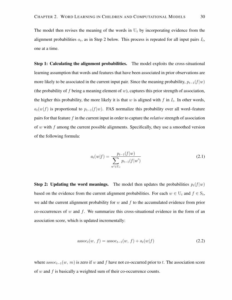
CHAPTER 2. WORD LEARNING IN CHILDREN AND COMPUTATIONAL MODELS 30
The model then revises the meaning of the words in Ut by incorporating evidence from the
alignment probabilities at, as in Step 2 below. This process is repeated for all input pairs It,
one at a time.
Step 1: Calculating the alignment probabilities. The model exploits the cross-situational
learning assumption that words and features that have been associated in prior observations are
more likely to be associated in the current input pair. Since the meaning probability, pt−1(f |w)
(the probability of f being a meaning element of w), captures this prior strength of association,
the higher this probability, the more likely it is that w is aligned with f in It. In other words,
at(w|f) is proportional to pt−1(f |w). FAS normalize this probability over all word–feature
pairs for that feature f in the current input in order to capture the relative strength of association
of w with f among the current possible alignments. Specifically, they use a smoothed version
of the following formula:
at(w |f ) =pt−1(f |w)∑
w ′∈Ut
pt−1(f |w ′)(2.1)
Step 2: Updating the word meanings. The model then updates the probabilities pt(f |w)
based on the evidence from the current alignment probabilities. For each w ∈ Ut and f ∈ St,
we add the current alignment probability for w and f to the accumulated evidence from prior
co-occurrences of w and f . We summarize this cross-situational evidence in the form of an
association score, which is updated incrementally:
assoct(w, f) = assoct−1(w, f) + at(w|f) (2.2)
where assoct−1(w, m) is zero if w and f have not co-occurred prior to t. The association score
of w and f is basically a weighted sum of their co-occurrence counts.
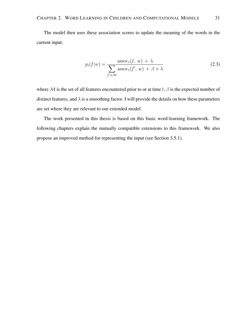
CHAPTER 2. WORD LEARNING IN CHILDREN AND COMPUTATIONAL MODELS 31
The model then uses these association scores to update the meaning of the words in the
current input:
pt(f |w) =assoct(f , w) + λ∑
f ′∈M
assoct(f′, w) + β × λ
(2.3)
whereM is the set of all features encountered prior to or at time t, β is the expected number of
distinct features, and λ is a smoothing factor. I will provide the details on how these parameters
are set where they are relevant to our extended model.
The work presented in this thesis is based on this basic word-learning framework. The
following chapters explain the mutually compatible extensions to this framework. We also
propose an improved method for representing the input (see Section 3.5.1).
Chapter 3
Individual Differences in Word Learning
3.1 Background on Late Talking
While most children are very efficient word learners, some show substantial delay. Late talkers
(LTs) are children at an early stage who are on a markedly slower path of vocabulary learning,
without evidence of any specific cognitive deficits. Although many LTs eventually catch up
to their age-matched peers, some continue on a slower path of learning, and at some point
in development are considered as exhibiting specific language impairment (SLI) (Thal et al.,
1997; Desmarais et al., 2008).1 Early identification of children at risk for SLI is very important,
since early intervention is key to alleviating its effects. Because late talking can be an early
sign of SLI, many psycholinguistic studies have focused on understanding its properties (e.g.,
Weismer and Evans, 2002; Paul and Elwood, 1991).
Research has shown that LTs exhibit not only a delay in vocabulary learning, but a slower
learning rate as well (e.g., Weismer and Evans, 2002). Moreover, an important observation
about late-talking children is that they learn differently from their normally-developing (ND)
peers. For example, the vocabulary composition of LTs shows greater variability, e.g., in terms
1There is evidence on the role of genetics in language disorders: Having a family history of specific languageimpairment is more common among children with the disorder than normally-developing ones. However, nospecific genes are known to cause SLI (Stromswold, 2008).
32
CHAPTER 3. INDIVIDUAL DIFFERENCES IN WORD LEARNING 33
of how consistently certain properties, such as shape, are associated with particular categories,
such as solid objects (Jones and Smith, 2005; Colunga and Sims, 2011). More generally, the
vocabulary of LTs has been shown to exhibit less semantic connectivity than that of NDs (Sheng
and McGregor, 2010; Beckage et al., 2010). In this thesis, “semantic connectivity” refers to the
overall pattern of semantic similarity among the learner’s vocabulary items. Throughout the
thesis, semantic connectivity is quantified in various ways as appropriate to each experiment.
Numerous factors may contribute to late talking, including environmental conditions, such
as the quantity or quality of the linguistic input (Paul and Elwood, 1991; Rowe, 2008), as
well as cognitive abilities of the learner, such as differences in categorization skills, working
memory, or attentional abilities (Jones and Smith, 2005; Stokes and Klee, 2009; Rescorla and
Merrin, 1998). These studies suggest that different cognitive and environmental factors might
contribute to late talking; but, it is not clear how these factors contribute to the patterns observed
in word learning of late talkers and normally developing learners. Computational modeling is
necessary for investigating precise proposals of how such a variety of complex environmental
and/or cognitive factors can interact in the process of vocabulary learning. However, to our
knowledge, there are no previous computational models of word learning in context demon-
strating the effects of possible factors that contribute to late talking.
We propose a computational model that enables us to thoroughly examine one of the possi-
ble factors behind late talking, specifically, individual differences in attentional development.
Attention is generally defined as the ability to selectively focus on some aspects of the environ-
ment. In this thesis, attention refers to the process of concentrating on the aspects of a scene
that can facilitate learning. The literature provides evidence for individual differences in the
development of the ability of a learner to respond to joint attention (Morales et al., 2000). In
particular, late-talking children exhibit difficulty in using communicative cues and in initiating
joint attention with their partner (Paul and Shiffer, 1991; Rescorla and Merrin, 1998). Our
model incorporates an attentional mechanism that gradually improves over time, enabling it
to focus (more or less) on the features relevant to a word. We simulate normally-developing
CHAPTER 3. INDIVIDUAL DIFFERENCES IN WORD LEARNING 34
and late-talking learners by parameterizing the rate of development of this mechanism, such
that ND has a faster rate. Because the attentional mechanism impacts the learning algorithm of
the model, the ND and LT learners differ in the quality of their learned meanings. This prop-
erty of the model enables us to further investigate the differences in semantic connectivity and
structure of vocabulary of ND and LT learners. We also investigate the differences observed
in subgroups of late talkers, that is, those who eventually catch up with normally-developing
children and those who stay on a slower path of learning.
This chapter is organized as follows: Section 3.2 provides a detailed explanation of our
computational model in which we extend the model of Fazly et al. (2010b) presented in Sec-
tion 2.4. By modeling attentional development, we can replicate several patterns observed
in ND and LT’s word learning (Section 3.3). In Section 3.4, we extend the model to form
semantic categories from learned word meanings. This allows us to further shed light on dif-
ferences observed in ND and LT children by studying the interaction of categorization and
word learning. Section 3.5 focuses on our experimental findings on the role of categorization
in individual differences in word learning. In Section 3.6, we explain the behavioral data on
the structural differences in ND and LT’s vocabulary. Finally, we discuss our findings from
examining the structural properties of the vocabulary of ND and LT learners (Section 3.7). The
work presented in this chapter has been published in Nematzadeh et al. (2011) (Section 3.2 and
Section 3.3), Nematzadeh et al. (2012b) (Section 3.4 and Section 3.5), and Nematzadeh et al.
(2014a) (Section 3.6 and Section 3.7).
3.2 Modeling Changes in Attention over Time
It has been observed that children’s joint attention skills—which underlie their ability to fo-
cus on the intended meaning for a word—develop over time (Mundy et al., 2007). Here, we
propose an attentional mechanism that improves over time, and show how it can be varied in
computational experiments, corresponding to simulations of normally-developing children and
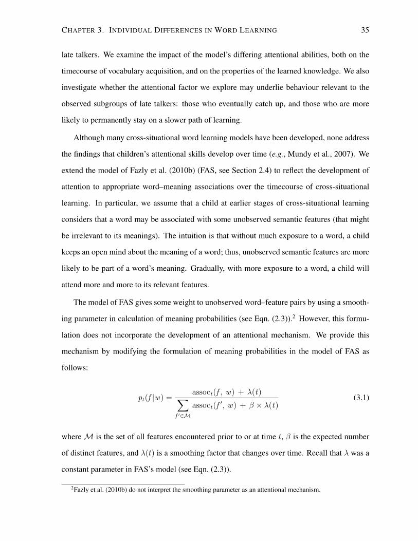
CHAPTER 3. INDIVIDUAL DIFFERENCES IN WORD LEARNING 35
late talkers. We examine the impact of the model’s differing attentional abilities, both on the
timecourse of vocabulary acquisition, and on the properties of the learned knowledge. We also
investigate whether the attentional factor we explore may underlie behaviour relevant to the
observed subgroups of late talkers: those who eventually catch up, and those who are more
likely to permanently stay on a slower path of learning.
Although many cross-situational word learning models have been developed, none address
the findings that children’s attentional skills develop over time (e.g., Mundy et al., 2007). We
extend the model of Fazly et al. (2010b) (FAS, see Section 2.4) to reflect the development of
attention to appropriate word–meaning associations over the timecourse of cross-situational
learning. In particular, we assume that a child at earlier stages of cross-situational learning
considers that a word may be associated with some unobserved semantic features (that might
be irrelevant to its meanings). The intuition is that without much exposure to a word, a child
keeps an open mind about the meaning of a word; thus, unobserved semantic features are more
likely to be part of a word’s meaning. Gradually, with more exposure to a word, a child will
attend more and more to its relevant features.
The model of FAS gives some weight to unobserved word–feature pairs by using a smooth-
ing parameter in calculation of meaning probabilities (see Eqn. (2.3)).2 However, this formu-
lation does not incorporate the development of an attentional mechanism. We provide this
mechanism by modifying the formulation of meaning probabilities in the model of FAS as
follows:
pt(f |w) =assoct(f , w) + λ(t)∑
f ′∈M
assoct(f′, w) + β × λ(t)
(3.1)
whereM is the set of all features encountered prior to or at time t, β is the expected number
of distinct features, and λ(t) is a smoothing factor that changes over time. Recall that λ was a
constant parameter in FAS’s model (see Eqn. (2.3)).
2Fazly et al. (2010b) do not interpret the smoothing parameter as an attentional mechanism.
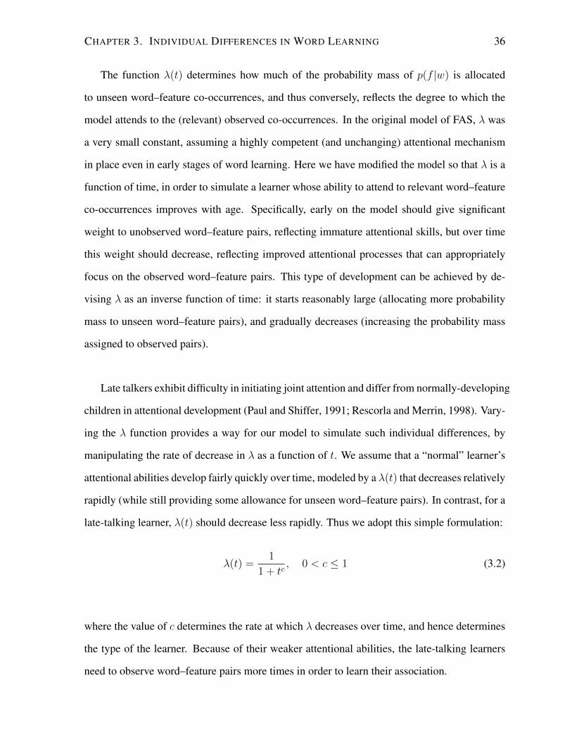
CHAPTER 3. INDIVIDUAL DIFFERENCES IN WORD LEARNING 36
The function λ(t) determines how much of the probability mass of p(f |w) is allocated
to unseen word–feature co-occurrences, and thus conversely, reflects the degree to which the
model attends to the (relevant) observed co-occurrences. In the original model of FAS, λ was
a very small constant, assuming a highly competent (and unchanging) attentional mechanism
in place even in early stages of word learning. Here we have modified the model so that λ is a
function of time, in order to simulate a learner whose ability to attend to relevant word–feature
co-occurrences improves with age. Specifically, early on the model should give significant
weight to unobserved word–feature pairs, reflecting immature attentional skills, but over time
this weight should decrease, reflecting improved attentional processes that can appropriately
focus on the observed word–feature pairs. This type of development can be achieved by de-
vising λ as an inverse function of time: it starts reasonably large (allocating more probability
mass to unseen word–feature pairs), and gradually decreases (increasing the probability mass
assigned to observed pairs).
Late talkers exhibit difficulty in initiating joint attention and differ from normally-developing
children in attentional development (Paul and Shiffer, 1991; Rescorla and Merrin, 1998). Vary-
ing the λ function provides a way for our model to simulate such individual differences, by
manipulating the rate of decrease in λ as a function of t. We assume that a “normal” learner’s
attentional abilities develop fairly quickly over time, modeled by a λ(t) that decreases relatively
rapidly (while still providing some allowance for unseen word–feature pairs). In contrast, for a
late-talking learner, λ(t) should decrease less rapidly. Thus we adopt this simple formulation:
λ(t) =1
1 + tc, 0 < c ≤ 1 (3.2)
where the value of c determines the rate at which λ decreases over time, and hence determines
the type of the learner. Because of their weaker attentional abilities, the late-talking learners
need to observe word–feature pairs more times in order to learn their association.
CHAPTER 3. INDIVIDUAL DIFFERENCES IN WORD LEARNING 37
3.3 Experiments on Attentional Development
As noted several key behaviours have been observed regarding the learning of word meanings
by LTs in comparison with their age-matched peers. First, LTs have both delayed vocabulary
learning and a slower learning rate; while some LTs catch up to their peers, others do not.
Second, LTs have more difficulty in learning novel words in an experimental setting. Third,
the learned words of LTs seem to have less strong semantic connectedness among them. In this
section, we present three corresponding sets of experiments demonstrating that variation in the
attention parameter in our model can lead to each of these behaviours observed in children.
3.3.1 Experimental Setup
Input Utterance–Scene Pairs
The input to the model consists of a sequence of utterance–scene pairs intended to reflect the
linguistic data a child is exposed to, along with the associated meaning a child might grasp. As
in much previous work (Yu and Ballard, 2007; Fazly et al., 2010b), we take child-directed utter-
ances from the CHILDES database (MacWhinney, 2000) in order to have naturalistic data. In
particular, we use the Manchester corpus (Theakston et al., 2001), which consists of transcripts
of conversations with 12 British children between the ages of 1; 8 and 3; 0. We represent each
utterance as a bag of lemmatized words. The data from half of the children is used as develop-
ment data (about 69, 000 utterances and 191, 000 words), and the rest for our final experiments
(about 77, 000 utterances and 223, 000 words).
For the scene representation, we have no large corpus to draw on that encodes the semantic
portion of language acquisition data.Yu and Ballard (2007) created a corpus by hand-coding
the objects and cues that were present in the environment, but that corpus is very small. Frank
et al. (2013) provide a larger manually annotated corpus (5000 utterances), but it is still very
small for longitudinal simulations of word learning. (Our corpus contains more than 100,000
utterances.) Moreover, the corpus of Frank et al. is limited because a considerable number of
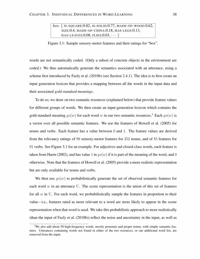
CHAPTER 3. INDIVIDUAL DIFFERENCES IN WORD LEARNING 38
box: IS-SQUARE:0.82, IS-SOLID:0.77, MADE-OF-WOOD:0.62,SIZE:0.4, MADE-OF-CHINA:0.18, HAS-LEGS:0.13,HAS-LEAVES:0.08, FLIES:0.03, · · ·
Figure 3.1: Sample sensory-motor features and their ratings for “box”.
words are not semantically coded. (Only a subset of concrete objects in the environment are
coded.) We thus automatically generate the semantics associated with an utterance, using a
scheme first introduced by Fazly et al. (2010b) (see Section 2.4.1). The idea is to first create an
input generation lexicon that provides a mapping between all the words in the input data and
their associated gold-standard meanings.
To do so, we draw on two semantic resources (explained below) that provide feature values
for different groups of words. We then create an input-generation lexicon which contains the
gold-standard meaning gs(w) for each word w in our two semantic resources.3 Each gs(w) is
a vector over all possible semantic features. We use the features of Howell et al. (2005) for
nouns and verbs. Each feature has a value between 0 and 1. The feature values are derived
from the relevancy ratings of 98 sensory-motor features for 352 nouns, and of 85 features for
91 verbs. See Figure 3.1 for an example. For adjectives and closed-class words, each feature is
taken from Harm (2002), and has value 1 in gs(w) if it is part of the meaning of the word, and 0
otherwise. Note that the features of Howell et al. (2005) provide a more realistic representation
but are only available for nouns and verbs.
We then use gs(w) to probabilistically generate the set of observed semantic features for
each word w in an utterance U. The scene representation is the union of this set of features
for all w in U. For each word, we probabilistically sample the features in proportion to their
value—i.e., features rated as more relevant to a word are more likely to appear in the scene
representation when that word is used. We take this probabilistic approach to more realistically
(than the input of Fazly et al. (2010b)) reflect the noise and uncertainty in the input, as well as
3We also add about 50 high-frequency words, mostly pronouns and proper nouns, with simple semantic fea-tures. Utterances containing words not found in either of the two resources, or our additional word list, areremoved from the input.
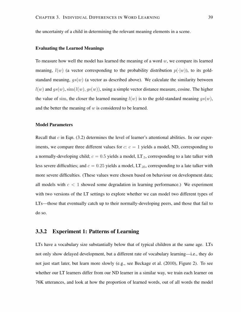
CHAPTER 3. INDIVIDUAL DIFFERENCES IN WORD LEARNING 39
the uncertainty of a child in determining the relevant meaning elements in a scene.
Evaluating the Learned Meanings
To measure how well the model has learned the meaning of a word w, we compare its learned
meaning, l(w) (a vector corresponding to the probability distribution p(·|w)), to its gold-
standard meaning, gs(w) (a vector as described above). We calculate the similarity between
l(w) and gs(w), sim(l(w), gs(w)), using a simple vector distance measure, cosine. The higher
the value of sim, the closer the learned meaning l(w) is to the gold-standard meaning gs(w),
and the better the meaning of w is considered to be learned.
Model Parameters
Recall that c in Eqn. (3.2) determines the level of learner’s attentional abilities. In our exper-
iments, we compare three different values for c: c = 1 yields a model, ND, corresponding to
a normally-developing child; c = 0.5 yields a model, LT.5, corresponding to a late talker with
less severe difficulties; and c = 0.25 yields a model, LT.25, corresponding to a late talker with
more severe difficulties. (These values were chosen based on behaviour on development data;
all models with c < 1 showed some degradation in learning performance.) We experiment
with two versions of the LT settings to explore whether we can model two different types of
LTs—those that eventually catch up to their normally-developing peers, and those that fail to
do so.
3.3.2 Experiment 1: Patterns of Learning
LTs have a vocabulary size substantially below that of typical children at the same age. LTs
not only show delayed development, but a different rate of vocabulary learning—i.e., they do
not just start later, but learn more slowly (e.g., see Beckage et al. (2010), Figure 2). To see
whether our LT learners differ from our ND learner in a similar way, we train each learner on
76K utterances, and look at how the proportion of learned words, out of all words the model
CHAPTER 3. INDIVIDUAL DIFFERENCES IN WORD LEARNING 40
Figure 3.2: Proportion of noun/verb word types learned.
has been exposed to, changes over time. We restrict our attention here to nouns and verbs,
since we believe their semantic representation is more elaborated (and thus more realistic).
The vocabulary growth plots of the three learners, depicted in Figure 3.2, show interesting
differences in accord with the patterns seen in children. First, the two LT models not only lag
behind the ND model with respect to the onset of word learning, but also show a different rate
and pattern of vocabulary learning (a very marked difference in the LT.25 case). Whereas ND
shows a sharp increase in the rate of vocabulary learning early on — 60% of words are learned
by the time the model has received about 150 words — the two LT learners exhibit a slower
and more gradual growth rate. In addition, the two LT models differ from each other. As is
observed in children, some learners (as with LT.5) who start off slow catch up in vocabulary
learning, while others (as with LT.25) continue indefinitely to lag behind their age-matched
peers. This distinction is important to understand more fully, since the latter are at risk for SLI.
CHAPTER 3. INDIVIDUAL DIFFERENCES IN WORD LEARNING 41
3.3.3 Experiment 2: Novel Word Learning
To understand how the vocabulary learning process of LTs differs from that of typical children,
psycholinguists test the performance of the two groups in a contrived novel word learning
situation: An experimenter first introduces a novel word and its novel referent to the child,
and then examines the child’s knowledge of the target (novel) word through explicit tests of
comprehension and/or production.
Here, we simulate a simplified version of the novel word-learning experiment of Weismer
and Evans (2002). First, we train the model on some number of corpus inputs, simulating
a child’s normal word-learning experience. We then introduce a novel noun to the model in
several teaching trials as follows: As our novel noun, we randomly pick a noun that has not oc-
curred in the training utterances. To simulate use of the novel noun in natural utterances, we add
the noun to an actual (as yet unseen) utterance from the corpus, and add its probabilistically-
generated meaning to the corresponding scene. We train our ND and LT learners on 3 such
teaching utterance–scene pairs as usual.
To examine the novel word-learning ability of each learner, we repeat the above process
for 106 novel nouns, for 3 teaching trials, and for different amounts of prior training utter-
ances (here, 10K, 30K, or 60K), and test as follows. Note that since at each point in time the
model processes an utterance, we use time and number of processed utterances interchangeably
throughout the thesis.
Comprehension. To test comprehension of a recently-taught novel word, the experimenter
asks the child to find the referent of the novel word, when presented with the novel object
along with one or more familiar objects. Note that in our computational experimental setting,
the “object” corresponding to a word is its gold-standard meaning, gs(w) (i.e., there is no
distinction between the gold-standard meaning of a word and a referent corresponding to that
meaning). We pair each novel object gs(wN) with one familiar object gs(wF), and calculate
the likelihood of selecting each of these in response to wN as the stimulus. Specifically, we test
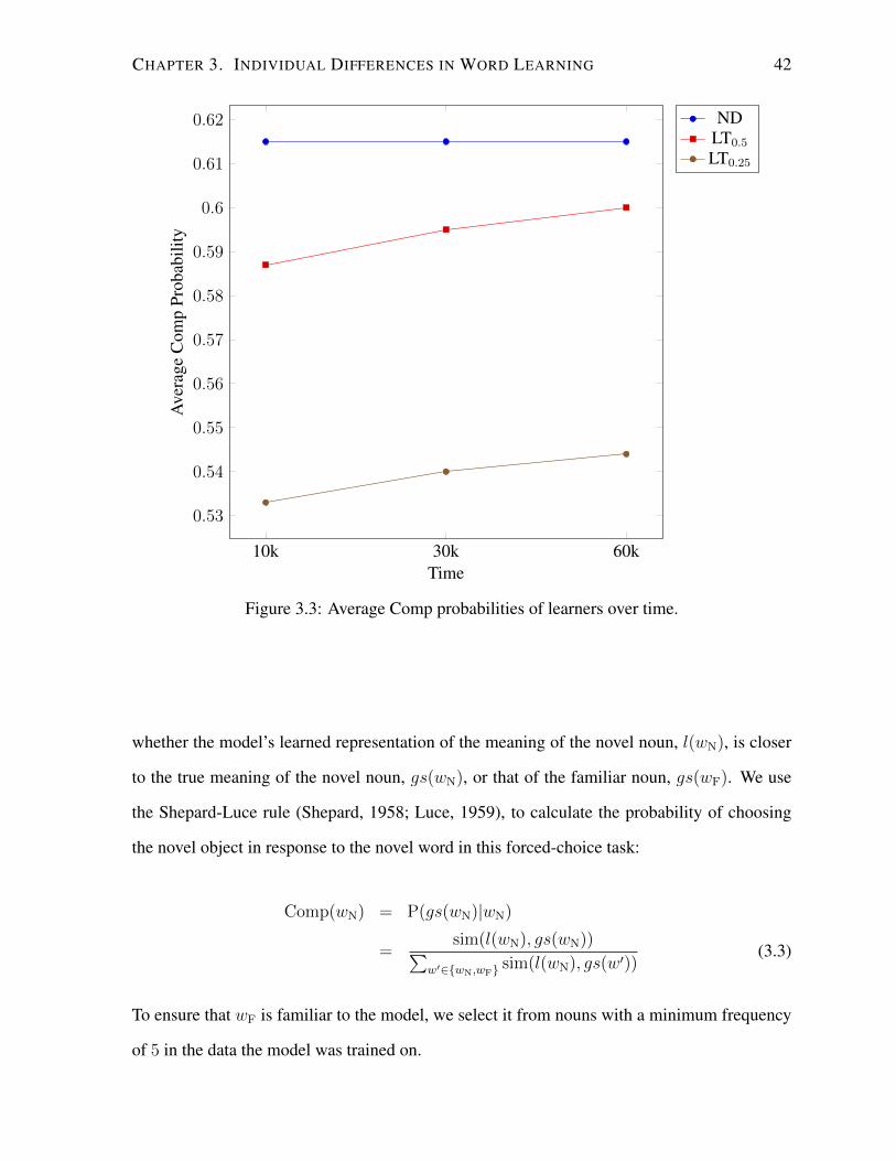
CHAPTER 3. INDIVIDUAL DIFFERENCES IN WORD LEARNING 42
10k 30k 60k
0.53
0.54
0.55
0.56
0.57
0.58
0.59
0.6
0.61
0.62
Time
Ave
rage
Com
pPr
obab
ility
NDLT0.5
LT0.25
Figure 3.3: Average Comp probabilities of learners over time.
whether the model’s learned representation of the meaning of the novel noun, l(wN), is closer
to the true meaning of the novel noun, gs(wN), or that of the familiar noun, gs(wF). We use
the Shepard-Luce rule (Shepard, 1958; Luce, 1959), to calculate the probability of choosing
the novel object in response to the novel word in this forced-choice task:
Comp(wN) = P(gs(wN)|wN)
=sim(l(wN), gs(wN))∑
w′∈wN,wF sim(l(wN), gs(w′))(3.3)
To ensure that wF is familiar to the model, we select it from nouns with a minimum frequency
of 5 in the data the model was trained on.
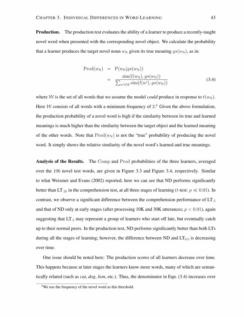
CHAPTER 3. INDIVIDUAL DIFFERENCES IN WORD LEARNING 43
Production. The production test evaluates the ability of a learner to produce a recently-taught
novel word when presented with the corresponding novel object. We calculate the probability
that a learner produces the target novel noun wN given its true meaning gs(wN), as in:
Prod(wN) = P(wN|gs(wN))
=sim(l(wN), gs(wN))∑w′∈W sim(l(w′), gs(wN))
(3.4)
whereW is the set of all words that we assume the model could produce in response to t(wN).
HereW consists of all words with a minimum frequency of 3.4 Given the above formulation,
the production probability of a novel word is high if the similarity between its true and learned
meanings is much higher than the similarity between the target object and the learned meaning
of the other words. Note that Prod(wN) is not the “true” probability of producing the novel
word. It simply shows the relative similarity of the novel word’s learned and true meanings.
Analysis of the Results. The Comp and Prod probabilities of the three learners, averaged
over the 106 novel test words, are given in Figure 3.3 and Figure 3.4, respectively. Similar
to what Weismer and Evans (2002) reported, here we can see that ND performs significantly
better than LT.25 in the comprehension test, at all three stages of learning (t-test: p 0.01). In
contrast, we observe a significant difference between the comprehension performance of LT.5
and that of ND only at early stages (after processing 10K and 30K utterances; p < 0.01), again
suggesting that LT.5 may represent a group of learners who start off late, but eventually catch
up to their normal peers. In the production test, ND performs significantly better than both LTs
during all the stages of learning; however, the difference between ND and LT0.5 is decreasing
over time.
One issue should be noted here: The production scores of all learners decrease over time.
This happens because at later stages the learners know more words, many of which are seman-
tically related (such as cat, dog, lion, etc.). Thus, the denominator in Eqn. (3.4) increases over
4We use the frequency of the novel word as this threshold.
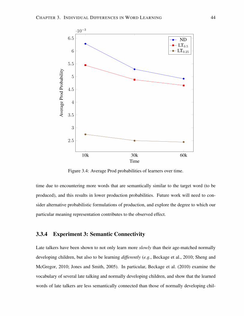
CHAPTER 3. INDIVIDUAL DIFFERENCES IN WORD LEARNING 44
10k 30k 60k
2.5
3
3.5
4
4.5
5
5.5
6
6.5
·10−3
Time
Ave
rage
Prod
Prob
abili
ty
NDLT0.5
LT0.25
Figure 3.4: Average Prod probabilities of learners over time.
time due to encountering more words that are semantically similar to the target word (to be
produced), and this results in lower production probabilities. Future work will need to con-
sider alternative probabilistic formulations of production, and explore the degree to which our
particular meaning representation contributes to the observed effect.
3.3.4 Experiment 3: Semantic Connectivity
Late talkers have been shown to not only learn more slowly than their age-matched normally
developing children, but also to be learning differently (e.g., Beckage et al., 2010; Sheng and
McGregor, 2010; Jones and Smith, 2005). In particular, Beckage et al. (2010) examine the
vocabulary of several late talking and normally developing children, and show that the learned
words of late talkers are less semantically connected than those of normally developing chil-
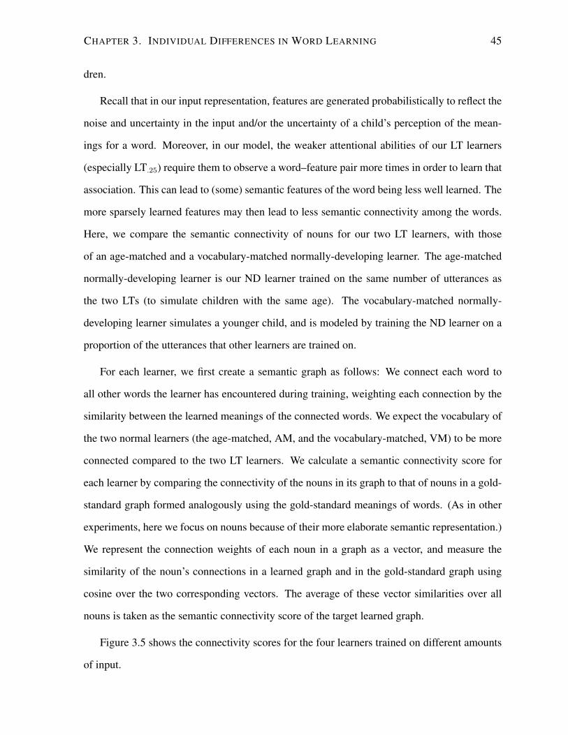
CHAPTER 3. INDIVIDUAL DIFFERENCES IN WORD LEARNING 45
dren.
Recall that in our input representation, features are generated probabilistically to reflect the
noise and uncertainty in the input and/or the uncertainty of a child’s perception of the mean-
ings for a word. Moreover, in our model, the weaker attentional abilities of our LT learners
(especially LT.25) require them to observe a word–feature pair more times in order to learn that
association. This can lead to (some) semantic features of the word being less well learned. The
more sparsely learned features may then lead to less semantic connectivity among the words.
Here, we compare the semantic connectivity of nouns for our two LT learners, with those
of an age-matched and a vocabulary-matched normally-developing learner. The age-matched
normally-developing learner is our ND learner trained on the same number of utterances as
the two LTs (to simulate children with the same age). The vocabulary-matched normally-
developing learner simulates a younger child, and is modeled by training the ND learner on a
proportion of the utterances that other learners are trained on.
For each learner, we first create a semantic graph as follows: We connect each word to
all other words the learner has encountered during training, weighting each connection by the
similarity between the learned meanings of the connected words. We expect the vocabulary of
the two normal learners (the age-matched, AM, and the vocabulary-matched, VM) to be more
connected compared to the two LT learners. We calculate a semantic connectivity score for
each learner by comparing the connectivity of the nouns in its graph to that of nouns in a gold-
standard graph formed analogously using the gold-standard meanings of words. (As in other
experiments, here we focus on nouns because of their more elaborate semantic representation.)
We represent the connection weights of each noun in a graph as a vector, and measure the
similarity of the noun’s connections in a learned graph and in the gold-standard graph using
cosine over the two corresponding vectors. The average of these vector similarities over all
nouns is taken as the semantic connectivity score of the target learned graph.
Figure 3.5 shows the connectivity scores for the four learners trained on different amounts
of input.
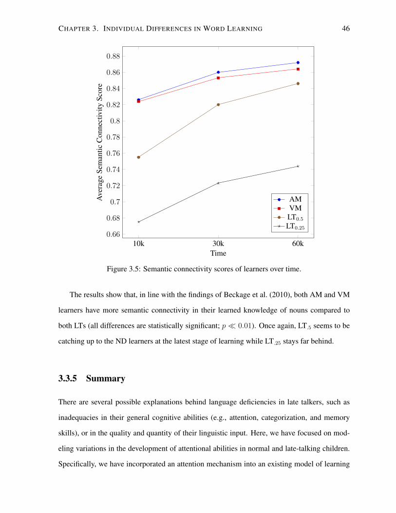
CHAPTER 3. INDIVIDUAL DIFFERENCES IN WORD LEARNING 46
10k 30k 60k0.66
0.68
0.7
0.72
0.74
0.76
0.78
0.8
0.82
0.84
0.86
0.88
Time
Ave
rage
Sem
antic
Con
nect
ivity
Scor
e
AMVMLT0.5
LT0.25
Figure 3.5: Semantic connectivity scores of learners over time.
The results show that, in line with the findings of Beckage et al. (2010), both AM and VM
learners have more semantic connectivity in their learned knowledge of nouns compared to
both LTs (all differences are statistically significant; p 0.01). Once again, LT.5 seems to be
catching up to the ND learners at the latest stage of learning while LT.25 stays far behind.
3.3.5 Summary
There are several possible explanations behind language deficiencies in late talkers, such as
inadequacies in their general cognitive abilities (e.g., attention, categorization, and memory
skills), or in the quality and quantity of their linguistic input. Here, we have focused on mod-
eling variations in the development of attentional abilities in normal and late-talking children.
Specifically, we have incorporated an attention mechanism into an existing model of learning
CHAPTER 3. INDIVIDUAL DIFFERENCES IN WORD LEARNING 47
word meanings in context, enabling us to model both a learner’s cognitive development over
time, as well as some individual differences among learners in lexical development.
Results of our experiments comparing the late-talking (LT) and normally-developing (ND)
models are compatible with the psycholinguistic findings: Compared to our ND model, the
LT model with severe difficulties (LT.25) exhibits marked delay in the onset of vocabulary
learning, performs significantly worse in learning novel words, and has less strong semantic
connections among its learned words. In contrast, the LT.5 learner (with less severe difficulties)
is significantly different from ND only at earlier stages of development, reflecting some normal
degree of variation in vocabulary learning.
The greater variability and the weaker connectivity in the vocabulary of LTs call for further
investigation since they might be reflective of underlying cognitive deficits in these children.
Psycholinguistic evidence suggests that children’s word learning improves when they form
some abstract knowledge about what kinds of semantic properties are relevant to what kinds
of categories (Jones et al., 1991; Colunga and Smith, 2005; Colunga and Sims, 2011). This
abstract knowledge is argued to emerge by generalizing over the learned words. Stated other-
wise, words that have been learned contribute to generalized abstract knowledge about word
meanings and semantic categories, which then guide subsequent word learning.
Late talkers have been shown to do worse in explicit word association tasks (Sheng and
McGregor, 2010), as well as in recognizing abstract categories (e.g., Jones and Smith, 2005;
Colunga and Sims, 2011). It is possible that because of the differences in the vocabulary
composition of LTs and NDs, the two groups of children also form different abstract knowledge
of categories, which causes differences in their word learning.
In the next section, we add explicit categorization abilities to our model, which enables
us to further investigate the differences of our various learners, both in capturing the semantic
connections among words, and in using these connections to bootstrap word learning. As in
Section 3.2, we simulate the difference between ND and LT learners as a difference in the
ability of the cross-situational learning mechanism to attend to appropriate semantic features
CHAPTER 3. INDIVIDUAL DIFFERENCES IN WORD LEARNING 48
for a word. Within this framework, we propose a new model that forms clusters of words
according to their learned semantic properties, and that uses this knowledge in guiding the
future associations between words and meanings.
3.4 Learning Semantic Categories of Words
We extend the word learning model explained in Section 3.2 by incorporating the ability to
form clusters of words based on their learned semantics, and to use the resulting semantic
categories in subsequent word learning.5 These abilities represent a first step in integrating the
model’s word learning with formation of conceptual categories. These extensions to the model
are key to further examination of the cognitive mechanisms that might underlie the weaker
semantic connectivity observed in the vocabulary of LTs. Specifically, while we showed (see
Section 3.3) that learned words of the ND learner had greater semantic coherence than those
in the LT learner, the model did not actually form semantic clusters of words, nor use semantic
relations among words to help in word learning.
Our new model, at given points in time, groups the words it has observed into clusters
based on the similarity among their learned meanings. Given two words w and w′, we deter-
mine their degree of semantic similarity by treating their learned probability distributions over
the semantic features, p(·|w) and p(·|w′), as input vectors to the cosine function. These co-
sine values guide the grouping of words using a standard unsupervised hierarchical clustering
method. The clusters of semantically related words can then be analyzed to see how the factors
that simulate ND and LT learners in the model contribute to different quality levels of semantic
categorization, as observed by Sheng and McGregor (2010) and Beckage et al. (2010), among
others.
Moreover, the semantic clusters enable us to build further on the explanation of late talk-
5We refer to the clusters that our model learns both as clusters, to emphasize that they are learned in an unsu-pervised manner, and as semantic categories, to emphasize their connection to children’s knowledge of abstractcategories.
CHAPTER 3. INDIVIDUAL DIFFERENCES IN WORD LEARNING 49
ing as arising from attentional differences in learners. Specifically, we assume that learned
semantic categories enable children to generalize their knowledge of related words, which can
help focus subsequent word learning on relevant semantic features in the input. In our model,
knowledge about the semantic category of a word can be used as an additional source of infor-
mation about which semantic features are more likely to be aligned with the word in a given
input. For example, features such as EDIBLE and FOOD should be more strongly aligned to a
word referring to a kind of fruit than to a word referring to a kind of vehicle.
We achieve this in our model by aligning a word w and a feature f in an input utterance–
scene pair according to both word-level and category-level information, the latter drawing on
the incrementally created semantic clusters. We adopt the formulation used by Alishahi and
Fazly (2010) to combine word and category information in the alignment probability:6
at(w|f) = Ω · aw,t(w|f) + (1− Ω) · ac,t(w|f) (3.5)
The first component of the above formula, aw,t(w|f) is the word-based alignment, given in
Eqn. (2.1) in Section 2.4. The second component, ac,t(w|f), is an analogous category-based
alignment (described below). The Ω term is a weight (between 0 and 1) that determines the
relative contribution of the two alignments; here we use a balanced weighting of 0.5.
Where the word-based alignment captures the association between a feature f and a single
word w, the category-based alignment, ac,t(w|f), assesses the overall association between f
and all the words in cluster(w), the cluster assignment determined by the model for w. The
category-based alignment is especially helpful when w is learned well enough to be clustered
with similar words, but its association with f is not informative. In this case, the association
of f with words that are similar to w (and thus are in the same cluster) can provide additional
information. The category-based alignment is calculated similar to the word-based alignment
6The approach of Alishahi and Fazly (2010) differs from ours: (1) They examine the role of syntactic cat-egories (e.g., noun or verb) in word learning while we look at semantic categories. (2) They use predefinedcorrect assignments of words to such parts of speech, but our clustering is based on the model’s learned semanticknowledge.
CHAPTER 3. INDIVIDUAL DIFFERENCES IN WORD LEARNING 50
(first introduced in Eqn. (2.1)) with occurrences of p(f |w) replaced with p(f |cluster(w)):
aw ,t(w |f ) =pt−1(f |w)∑
w ′∈Ut
pt−1(f |w ′)(3.6)
We follow Alishahi and Fazly (2010) in defining p(f |cluster(w)) as the average of the meaning
probabilities of the words in the cluster:
pt(f |cluster(w)) =1
|cluster(w)|∑
w∈cluster(w)
pt(f |w) (3.7)
where |cluster(w)| is the number of words in the cluster.
3.5 Experiments on Categorization
In Section 3.3, we showed in computational simulations that LT learners not only learn fewer
words than an ND learner, but that the LTs also have a less semantically-connected vocabulary,
a result in line with the findings of Beckage et al. (2010). Here, using our extended model with
its improved semantic representation, we analyze the learned clusters of words for our two
learners, to confirm that the semantic category knowledge of the LT learner is of substantially
poorer quality. We also investigate the differential effects of the learned clusters for the two
learners in subsequent word learning. It is known that word learning in children is boosted by
their knowledge of word categories (Jones et al., 1991). Here, we interleave the two processes
of semantic clustering and word learning in our model, and examine the patterns of word
learning over time, for the two learners, with and without category knowledge. Our hypothesis
is that the ND learner not only forms higher quality semantic clusters of words compared to
the LT learner, but that its (more coherent) category knowledge contributes to improved word
learning over time. We first provide details on how the experiments are set up and then discuss
their results.
CHAPTER 3. INDIVIDUAL DIFFERENCES IN WORD LEARNING 51
3.5.1 Experimental Setup
The input data used in the following experiments is the same as that of Section 3.3.1, ex-
cept we use an improved representation for nouns and verbs which is explained below. Sec-
tion 3.3.1 used a psycholinguistically-plausible set of features to represent nouns and verbs
(Howell et al., 2005); however, they were only available for a limited number of words. The
proposed representation does not impose this constraint, and thus results in a larger dataset with
more diverse vocabulary. Our development and test data consist of about 121, 000/481, 000 and
138, 000/556, 000 utterances/words respectively.
The Representation of Word Meaning
We focus on the semantics of nouns, since they are central to work on the role of category
knowledge in word learning. Here we develop an improved semantic representation for nouns
that enables a more extensive test of our clustering method and associated processing involving
semantic relatedness among words.
We construct the lexical entry gs(w) for each noun w drawing on WordNet7 as follows.
For each synset in WordNet, we select one member word to serve as the semantic feature
representing that synset. The initial representation of gs(w) consists of the set of such features
from each ancestor (hypernym) of the word’s first sense in WordNet.8 For verbs, we follow
Alishahi and Fazly (2010) in using features from WordNet as well as from a verb-specific
resource, VerbNet.9 We use the same features as in Section 3.3.1 to initialize gs(w) for other
parts of speech.
To complete the representation of gs(w), we need a score for each feature which can be
used in the probabilistic generation of a scene for an utterance containing w. We assume
7http://wordnet.princeton.edu8A native speaker of English annotated a sample of 500 nouns with their most relevant sense in our CDS
corpus, revealing that the first WordNet sense was appropriate for 80% of the nouns. One regular exception wasnouns with both ‘plant’ and ‘food’ senses, such as broccoli, which were predominantly referring to food. Forthese, we always use the ‘food’ sense.
9http://verbs.colorado.edu/˜mpalmer/projects/verbnet.htm
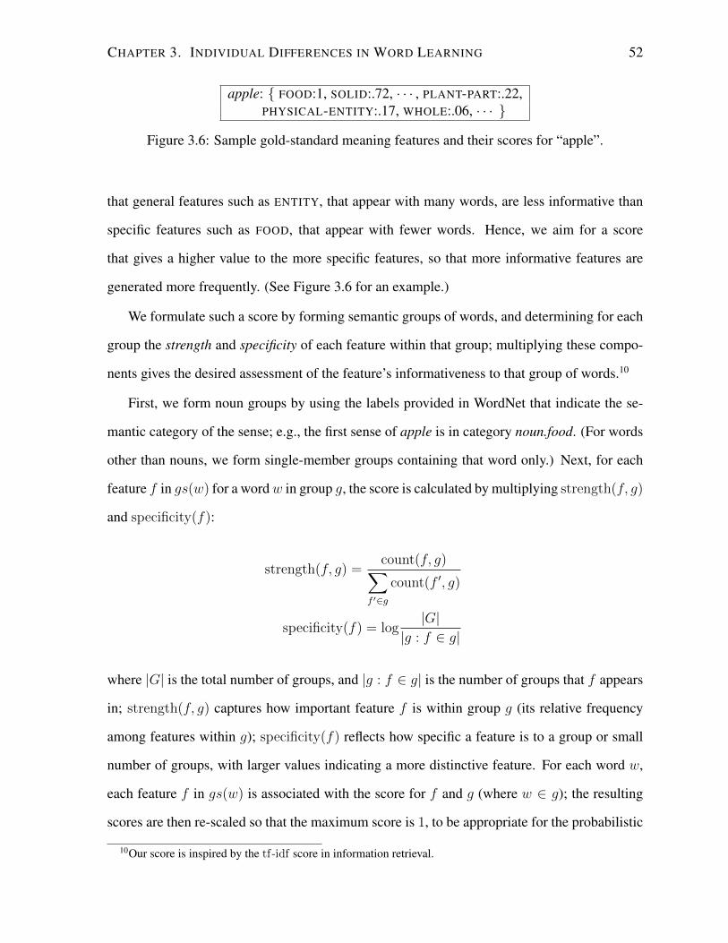
CHAPTER 3. INDIVIDUAL DIFFERENCES IN WORD LEARNING 52
apple: FOOD:1, SOLID:.72, · · · , PLANT-PART:.22,PHYSICAL-ENTITY:.17, WHOLE:.06, · · ·
Figure 3.6: Sample gold-standard meaning features and their scores for “apple”.
that general features such as ENTITY, that appear with many words, are less informative than
specific features such as FOOD, that appear with fewer words. Hence, we aim for a score
that gives a higher value to the more specific features, so that more informative features are
generated more frequently. (See Figure 3.6 for an example.)
We formulate such a score by forming semantic groups of words, and determining for each
group the strength and specificity of each feature within that group; multiplying these compo-
nents gives the desired assessment of the feature’s informativeness to that group of words.10
First, we form noun groups by using the labels provided in WordNet that indicate the se-
mantic category of the sense; e.g., the first sense of apple is in category noun.food. (For words
other than nouns, we form single-member groups containing that word only.) Next, for each
feature f in gs(w) for a wordw in group g, the score is calculated by multiplying strength(f, g)
and specificity(f):
strength(f, g) =count(f, g)∑
f ′∈g
count(f ′, g)
specificity(f) = log|G|
|g : f ∈ g|
where |G| is the total number of groups, and |g : f ∈ g| is the number of groups that f appears
in; strength(f, g) captures how important feature f is within group g (its relative frequency
among features within g); specificity(f) reflects how specific a feature is to a group or small
number of groups, with larger values indicating a more distinctive feature. For each word w,
each feature f in gs(w) is associated with the score for f and g (where w ∈ g); the resulting
scores are then re-scaled so that the maximum score is 1, to be appropriate for the probabilistic
10Our score is inspired by the tf-idf score in information retrieval.
CHAPTER 3. INDIVIDUAL DIFFERENCES IN WORD LEARNING 53
generation of the input scenes.
Model Parameters
In the next section, we report the results for two ND and LT learners. The ND and LT simula-
tions use the same settings for λ(t) (Eqn. (3.2)) as what we referred to as ND (i.e., c = 1) and
LT.5 (i.e., c = 0.5) in Section 3.3.1. Here, we only focus on the stronger LT learner (LT.5 as
opposed to LT.25). Because the vocabulary of LT0.25 is very weakly connected, it is not possible
to form meaningful categories (that can be helpful in word learning) over its words.
3.5.2 Experiment 1: Analysis of the Learned Clusters
We examine the quality of the semantic clusters formed by each learner (ND and LT). We
train the learners on 15K utterance–scene pairs, and perform a hierarchical clustering on the
resulting learned meanings of all the observed nouns. To provide a realistic upperbound as a
point of comparison for the two learners, we also cluster (using the same clustering algorithm
and similarity measure) the gold-standard meanings of the nouns. These “GOLD” clusters
indicate how well the nouns can be categorized by the clustering method on the basis of their
gold-standard (in contrast to learned) meanings. In all cases, we set the number of clusters to
20, which is the approximate number of the actual WordNet categories for nouns.
To measure the overall goodness of each of the three sets of clusters (GOLD, ND, and LT),
we compare the clustering to the actual WordNet category labels for the nouns, as follows.
(The WordNet category labels reflect human judgments of semantic categories, since they are
provided by manual annotation.) We first label each cluster c with the most frequent category
assigned by WordNet to the words in that cluster, called label(c). We then measure P(recision),
R(ecall), and their harmonic mean, F(-score), for each cluster, and average these over all clus-
ters in a set. Given a cluster c, P measures the fraction of nouns in c whose WordNet category
matches the cluster label; R is the fraction of all nouns whose WordNet category is label(c)
that are also in c. We report the average P, R, and F scores for the GOLD, LT, and ND clusters
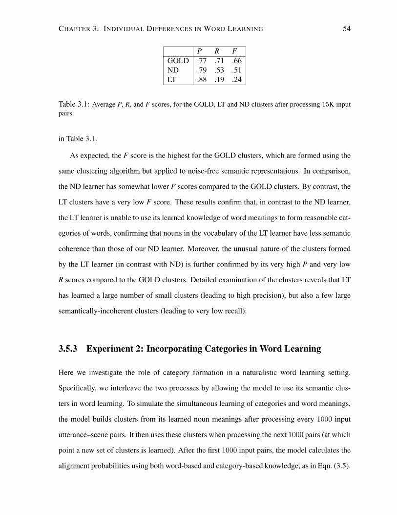
CHAPTER 3. INDIVIDUAL DIFFERENCES IN WORD LEARNING 54
P R FGOLD .77 .71 .66ND .79 .53 .51LT .88 .19 .24
Table 3.1: Average P, R, and F scores, for the GOLD, LT and ND clusters after processing 15K inputpairs.
in Table 3.1.
As expected, the F score is the highest for the GOLD clusters, which are formed using the
same clustering algorithm but applied to noise-free semantic representations. In comparison,
the ND learner has somewhat lower F scores compared to the GOLD clusters. By contrast, the
LT clusters have a very low F score. These results confirm that, in contrast to the ND learner,
the LT learner is unable to use its learned knowledge of word meanings to form reasonable cat-
egories of words, confirming that nouns in the vocabulary of the LT learner have less semantic
coherence than those of our ND learner. Moreover, the unusual nature of the clusters formed
by the LT learner (in contrast with ND) is further confirmed by its very high P and very low
R scores compared to the GOLD clusters. Detailed examination of the clusters reveals that LT
has learned a large number of small clusters (leading to high precision), but also a few large
semantically-incoherent clusters (leading to very low recall).
3.5.3 Experiment 2: Incorporating Categories in Word Learning
Here we investigate the role of category formation in a naturalistic word learning setting.
Specifically, we interleave the two processes by allowing the model to use its semantic clus-
ters in word learning. To simulate the simultaneous learning of categories and word meanings,
the model builds clusters from its learned noun meanings after processing every 1000 input
utterance–scene pairs. It then uses these clusters when processing the next 1000 pairs (at which
point a new set of clusters is learned). After the first 1000 input pairs, the model calculates the
alignment probabilities using both word-based and category-based knowledge, as in Eqn. (3.5).
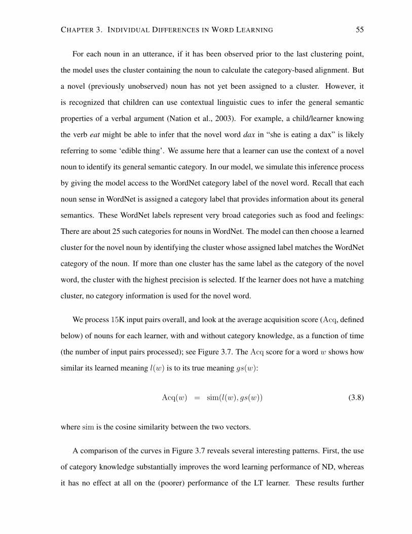
CHAPTER 3. INDIVIDUAL DIFFERENCES IN WORD LEARNING 55
For each noun in an utterance, if it has been observed prior to the last clustering point,
the model uses the cluster containing the noun to calculate the category-based alignment. But
a novel (previously unobserved) noun has not yet been assigned to a cluster. However, it
is recognized that children can use contextual linguistic cues to infer the general semantic
properties of a verbal argument (Nation et al., 2003). For example, a child/learner knowing
the verb eat might be able to infer that the novel word dax in “she is eating a dax” is likely
referring to some ‘edible thing’. We assume here that a learner can use the context of a novel
noun to identify its general semantic category. In our model, we simulate this inference process
by giving the model access to the WordNet category label of the novel word. Recall that each
noun sense in WordNet is assigned a category label that provides information about its general
semantics. These WordNet labels represent very broad categories such as food and feelings:
There are about 25 such categories for nouns in WordNet. The model can then choose a learned
cluster for the novel noun by identifying the cluster whose assigned label matches the WordNet
category of the noun. If more than one cluster has the same label as the category of the novel
word, the cluster with the highest precision is selected. If the learner does not have a matching
cluster, no category information is used for the novel word.
We process 15K input pairs overall, and look at the average acquisition score (Acq, defined
below) of nouns for each learner, with and without category knowledge, as a function of time
(the number of input pairs processed); see Figure 3.7. The Acq score for a word w shows how
similar its learned meaning l(w) is to its true meaning gs(w):
Acq(w) = sim(l(w), gs(w)) (3.8)
where sim is the cosine similarity between the two vectors.
A comparison of the curves in Figure 3.7 reveals several interesting patterns. First, the use
of category knowledge substantially improves the word learning performance of ND, whereas
it has no effect at all on the (poorer) performance of the LT learner. These results further
CHAPTER 3. INDIVIDUAL DIFFERENCES IN WORD LEARNING 56
Figure 3.7: Change in the average Acq score of all nouns over time (measured in number ofprocessed utterances); ND-CAT and LT-CAT use category information during learning.
elaborate the findings of our analysis of the learned clusters: the clusters learned by the ND
are a better match than those of the LT with the manually-annotated categories provided by
WordNet; moreover, they are able to contribute helpful information to word learning, where
the LT clusters are not.
Thus, the LT clusters are not only in principle of lesser quality, they are in practice less use-
ful. Also, the positive effect of category knowledge for ND increases over time, suggesting that
the quality of its clusters improves as the model is exposed to more input. This mutually rein-
forcing effect of semantic category formation with word learning underscores the importance
of studying the interaction of the two.
3.5.4 Experiment 3: Category Knowledge in Novel Word Learning
Results of the previous section suggest that the ability of a learner to form reliable categories of
semantically-similar words may be closely tied to its word learning performance. In particular,
CHAPTER 3. INDIVIDUAL DIFFERENCES IN WORD LEARNING 57
we expect category knowledge to increase the likelihood of associating a word with its relevant
semantic features when there is ambiguity and uncertainty in the cross-situational evidence.
For example, when a child hears “The wug will drink the dax” while observing an unknown
animal and a bowl of liquid in the scene, the child must rely on information sources other than
the cross-situational evidence to infer the possible meanings of the two novel words. (That is,
the child must infer that wug as a drinker is more likely to be the unknown animal.) We predict
a substantial benefit of category knowledge when observing a word for the first time, since this
is when there’s the least cross-situational information available to a learner about the particular
word and its features. Here we examine the effect of category knowledge on the learning of
novel words over time, within the naturalistic setting of the utterance–scene pairs of our corpus,
focusing on those inputs that include previously unseen words.
We train the model on 15K input pairs, but restrict evaluation to the learning of novel
words.11 Specifically, we look at the difference in the Acq score of words at their first exposure,
for the ND and LT learners, each with and without using category knowledge. To do this, we
look at utterances containing at least two nouns, at least one of which is novel.12 For each such
input utterance, we record the resulting Acq score of all novel words in the utterance, and take
their average. For each learner, we also examine the pattern of change in these average scores
over time, as shown in Figure 3.8.
The results show that after 2K input utterances, there is no difference between using and
not using categories for each of the learners (i.e., comparing ND-CAT and LT-CAT to ND and
LT, respectively). This is because none of the learners has formed sufficiently good categories
yet. After 8K utterances, ND-CAT performs much better than ND, showing the benefit of using
category knowledge in learning novel words in an ambiguous setting. By contrast, for the LT
learner, the Acq score of the novel nouns does not increase when using category information
(LT-CAT) even with additional exposure to the input. Another interesting pattern is that for the
11Note that the cluster of a novel word is determined using its WordNet category label as discussed in Sec-tion 3.5.3.
12If the utterance only has 1 novel noun, the task is too easy because the features of nouns and other parts ofspeech do not overlap.
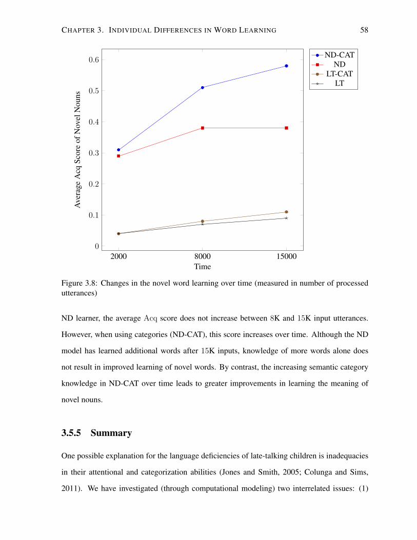
CHAPTER 3. INDIVIDUAL DIFFERENCES IN WORD LEARNING 58
2000 8000 150000
0.1
0.2
0.3
0.4
0.5
0.6
Time
Ave
rage
Acq
Scor
eof
Nov
elN
ouns
ND-CATND
LT-CATLT
Figure 3.8: Changes in the novel word learning over time (measured in number of processedutterances)
ND learner, the average Acq score does not increase between 8K and 15K input utterances.
However, when using categories (ND-CAT), this score increases over time. Although the ND
model has learned additional words after 15K inputs, knowledge of more words alone does
not result in improved learning of novel words. By contrast, the increasing semantic category
knowledge in ND-CAT over time leads to greater improvements in learning the meaning of
novel nouns.
3.5.5 Summary
One possible explanation for the language deficiencies of late-talking children is inadequacies
in their attentional and categorization abilities (Jones and Smith, 2005; Colunga and Sims,
2011). We have investigated (through computational modeling) two interrelated issues: (1)
CHAPTER 3. INDIVIDUAL DIFFERENCES IN WORD LEARNING 59
how variations in the development of attentional abilities in normally-developing (ND) and
late-talking (LT) children may interact with their categorization skills, and (2) how differences
in semantic category formation could affect word learning. We have extended our word learn-
ing model that incorporates an attention mechanism (see Section 3.2) to incrementally cluster
words, and to use these semantic clusters in subsequent word learning.
Psycholinguistic findings have noted that the vocabulary of LTs shows both a lack of ap-
propriate category-based generalization (Jones and Smith, 2005; Colunga and Sims, 2011),
and less semantic connectivity (Beckage et al., 2010; Sheng and McGregor, 2010). We find
here that the clusters formed by our LT model indeed show more inconsistency and less co-
herence than those of our ND learner. In addition, unlike our LT learner, our ND model can
use its learned knowledge of word meanings to form semantically-coherent and informative
categories, which in turn contribute to an improvement in subsequent word learning. More-
over, the LT learner has particular difficulties in learning novel words, while the ND learner
gets increasingly better over time when it draws on category knowledge. The inability of an
LT learner to form reasonable semantic clusters limits its ability to generalize its knowledge of
learned words to new words. This could be a substantial factor in the LT’s delayed vocabulary
acquisition.
The vocabulary of late talkers is not only less semantically-connected than that of normally-
developing children, but also exhibits a different structure (Beckage et al., 2010). The next
section provides a detailed explanation of the structural differences observed in LT and ND
children. In Section 3.7.3, we compare the structure of vocabulary of our ND and LT learners
to that of normally-developing and late-talking children.
3.6 Constructing a Learner’s Semantic Network
Semantic knowledge – word-to-concept mappings and the relations among the words and/or
concepts – is often represented as a semantic network in which the nodes correspond to words
CHAPTER 3. INDIVIDUAL DIFFERENCES IN WORD LEARNING 60
or concepts, and the edges specify semantic relationships among them (e.g., Collins and Loftus,
1975; Steyvers and Tenenbaum, 2005). Steyvers and Tenenbaum (2005) argue that semantic
networks created from adult-level knowledge of words exhibit a small-world and scale-free
structure: an overall sparse network with highly-connected local sub-networks, where these
sub-networks are connected through high-degree hubs (nodes with many neighbours). Through
mathematical modeling, they argue that these properties arise from the developmental process
of semantic network creation, in which word meanings are differentiated over time.
The work of Steyvers and Tenenbaum (2005) raises very interesting follow-on questions:
To what degree does children’s developing semantic knowledge of words exhibit a small-world
and scale-free structure? How do these properties arise from the process of vocabulary acquisi-
tion in children? The work of Beckage et al. (2011) is suggestive regarding these issues. They
compare semantic networks formed from the productive vocabulary of normally-developing
children and from that of late talkers. Beckage et al. (2011) show that the network of vo-
cabulary of late talkers exhibited a small-world structure to a lesser degree than that of the
normally-developing children. However, while this work suggests some preliminary answers
to the first question above, it cannot shed light on the relation between the process of word
learning and the small-world and scale-free properties. Specifically, the networks considered
by Beckage et al. (2011) only include productive vocabulary, not the many words a child will
have partial knowledge of, and the connections among the words are determined by using co-
occurrence statistics from a corpus, not the children’s own knowledge or use of the words.
In order to shed light on how the small-world and scale-free properties arise from the devel-
opmental process of word learning, we need to consider the structure of semantic networks
formed from the (partially) learned meanings of the words in the child’s environment.
Here we take advantage of our ND and LT models to examine the properties of semantic
networks that include all the vocabulary a learner has been exposed to (i.e., even those partially
learned), and that has connections based on the actual learned knowledge of those words. We
train each learner (ND and LT) on an identical sequence of utterance–scene pairs, and then use
CHAPTER 3. INDIVIDUAL DIFFERENCES IN WORD LEARNING 61
their learned lexicons to build a semantic network for each. Unlike Beckage et al. (2011), we
do not want to restrict the network to productive vocabulary, which eliminates much semantic
knowledge of the learner (e.g. Benedict, 1979; Woodward and Markman, 1998). We thus
assume all the words that the model has been exposed to during training are part of the learner’s
semantic network. This reflects our assumption that an important aspect of a learner’s semantic
knowledge is that it (perhaps imperfectly) captures connections among even words that cannot
yet be fully comprehended or produced.
To establish the connections among nodes in the network, we examine the semantic similar-
ity of the meanings of the corresponding words. Specifically, we measure semantic similarity
of two words by turning their meanings into vectors, and calculating the cosine of the angle
between the two vectors. We connect two nodes in the network if the similarity of their cor-
responding words is higher than a pre-defined threshold. This process yields two networks,
Net-ND and Net-LT, each of which contains nodes for all the words in the input, with the
edges determined by the semantic similarity of the word meanings represented within the ND
and LT learners, respectively. For comparison, we also build a gold-standard semantic network,
Net-GS, that contains the same words as Net-ND and Net-LT (i.e., all the words in the input),
but relies on the gold-standard meanings of words (from the gold-standard lexicon) to estab-
lish the connections. Note that the structure of this network does not depend on the learners’
knowledge of word meanings, but only on the similarity of the gold-standard meanings.
In order to further explore the importance of the knowledge of (partially) learned meanings
to the structure of the resulting networks, we also consider a variation on Net-ND and Net-
LT. Like Beckage et al. (2011), we can consider only a subset of the best-learned words of
the learners, and see whether the vocabulary itself – as opposed to what the learner has learned
about that vocabulary – exhibits the small-world and scale-free properties. Recall that Beckage
et al. (2011) create semantic networks connected on the basis of corpus-based co-occurrence
statistics that are the same for both groups of children – i.e., it is the make-up of the vocabulary,
rather than the learner’s knowledge of that vocabulary, that differs across the two types of
CHAPTER 3. INDIVIDUAL DIFFERENCES IN WORD LEARNING 62
networks. In our approach, this corresponds to using the gold-standard meanings from the
gold-standard lexicon to connect the words in the network.
Hence, we form additional networks, Net-NDacq and Net-LTacq as follows. We take “pro-
ductive” vocabulary in our model to be a subset of words which are learned better than a
predefined threshold (by comparing the learned meaning to the gold-standard meaning in the
gold-standard lexicon). We then build semantic networks that contain these acquired words of
our ND and LT learners, connected by drawing on the similarity of the gold-standard meanings
(that are the same for both learners). We can then use these networks to further explore the im-
portance of the partially learned knowledge of words in our original networks in contributing
to small-world and scale-free networks.
To summarize, we consider the following networks:
1. Net-GS: The nodes of the network are all the words in the input, and the edges are based
on the similarity of the gold-standard meanings of the words.
2. Net-ND and Net-LT: The nodes are all the words in the input, and the edges are based
on the similarity of the learned meanings of the words in each of the modeling scenarios.
3. Net-NDacq and Net-LTacq: The nodes are the acquired words (those best learned) in
each scenario, and the edges are based on the similarity of the gold-standard meanings
of those words.
3.7 Experiments on Semantic Networks
3.7.1 Evaluating the Networks’ Structural Properties
A network that exhibits a small-world structure has certain connectivity properties – short paths
and highly-connected neighborhoods – that are captured by various graph metrics (Watts and
Strogatz, 1998). Below we explain these properties, and how they are measured for a graph
CHAPTER 3. INDIVIDUAL DIFFERENCES IN WORD LEARNING 63
withN nodes andE edges. Then we explain the requirement for a network to yield a scale-free
structure.
Short paths between nodes. Most of the nodes of a small-world network are reachable
from other nodes via relatively short paths. For a connected network (i.e., all the node pairs
are reachable from each other), this can be measured as the average distance between all node
pairs (Watts and Strogatz, 1998). Since our networks are not connected, we instead measure
this property using the median of the distances (dmedian) between all node pairs (e.g., Robins
et al., 2005), which is well-defined even when some node pairs have a distance of∞.
Highly-connected neighborhoods. The neighborhood of a node n in a graph consists of n
and all of the nodes that are connected to it. A neighborhood is maximally connected if it forms
a complete graph —i.e., there is an edge between all node pairs. Thus, the maximum number
of edges in the neighborhood of n is kn(kn − 1)/2, where kn is the number of neighbors. A
standard metric for measuring the connectedness of neighbors of a node n is called the local
clustering coefficient (C) (Watts and Strogatz, 1998), which calculates the ratio of edges in the
neighborhood of n (En) to the maximum number of edges possible for that neighborhood:
C =En
kn(kn − 1)/2(3.9)
The local clustering coefficient C ranges between 0 and 1. To estimate the connectedness of
all neighborhoods in a network, we take the average of C over all nodes, i.e., Cavg.
Small-world structure. A graph exhibits a small-world structure if dmedian is relatively
small and Cavg is relatively high. To assess this for a graph g, these values are typically com-
pared to those of a random graph with the same number of nodes and edges as g (Watts and
Strogatz, 1998; Humphries and Gurney, 2008). The random graph is generated by randomly
rearranging the edges of the network under consideration (Erdos and Renyi, 1960). Because
any pair of nodes is equally likely to be connected as any other, the median of distances be-
tween nodes is expected to be low for a random graph. In a small-world network, this value
CHAPTER 3. INDIVIDUAL DIFFERENCES IN WORD LEARNING 64
dmedian is expected to be as small as that of a random graph: even though the random graph has
edges more uniformly distributed, the small-world network has many locally-connected com-
ponents which are connected via hubs. On the other hand, Cavg is expected to be much higher
in a small-world network compared to its corresponding random graph, because the edges of a
random graph typically do not fall into clusters forming highly connected neighborhoods.
Given these two properties, the “small-worldness” of a graph g is measured as follows
(Humphries and Gurney, 2008):
σg =
Cavg(g)
Cavg(random)
dmedian(g)
dmedian(random)
(3.10)
where random is the random graph corresponding to g. In a small-world network, it is ex-
pected that Cavg(g) Cavg(random) and dmedian(g) ≥ dmedian(random), and thus σg > 1.
Note that Steyvers and Tenenbaum (2005) made the empirical observation that small-world
networks of adult semantic knowledge had a single connected component that contained the
majority of nodes in the network. Thus, in addition to σg, we also measure the relative size of
a network’s largest connected component having size Nlcc:
sizelcc =Nlcc
N(3.11)
Scale-free structure. A scale-free network has a relatively small number of high-degree
nodes that have a large number of connections to other nodes, while most of its nodes have a
small degree, as they are only connected to a few nodes. Thus, if a network has a scale-free
structure, its degree distribution (i.e., the probability distribution of degrees over the whole
network) will follow a power-law distribution (which is said to be “scale-free”). We evaluate
this property of a network by plotting its degree distribution in the logarithmic scale, which (if
a power-law distribution) should appear as a straight line.
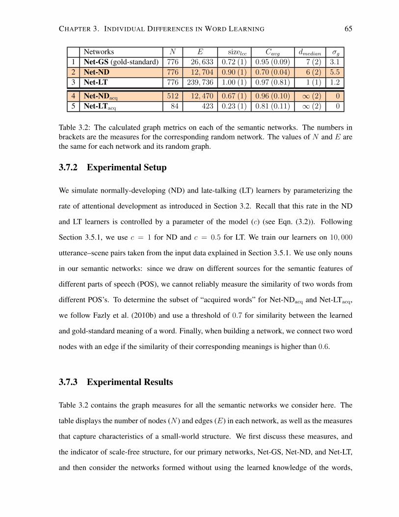
CHAPTER 3. INDIVIDUAL DIFFERENCES IN WORD LEARNING 65
Networks N E sizelcc Cavg dmedian σg1 Net-GS (gold-standard) 776 26, 633 0.72 (1) 0.95 (0.09) 7 (2) 3.1
2 Net-ND 776 12, 704 0.90 (1) 0.70 (0.04) 6 (2) 5.5
3 Net-LT 776 239, 736 1.00 (1) 0.97 (0.81) 1 (1) 1.2
4 Net-NDacq 512 12, 470 0.67 (1) 0.96 (0.10) ∞ (2) 0
5 Net-LTacq 84 423 0.23 (1) 0.81 (0.11) ∞ (2) 0
Table 3.2: The calculated graph metrics on each of the semantic networks. The numbers inbrackets are the measures for the corresponding random network. The values of N and E arethe same for each network and its random graph.
3.7.2 Experimental Setup
We simulate normally-developing (ND) and late-talking (LT) learners by parameterizing the
rate of attentional development as introduced in Section 3.2. Recall that this rate in the ND
and LT learners is controlled by a parameter of the model (c) (see Eqn. (3.2)). Following
Section 3.5.1, we use c = 1 for ND and c = 0.5 for LT. We train our learners on 10, 000
utterance–scene pairs taken from the input data explained in Section 3.5.1. We use only nouns
in our semantic networks: since we draw on different sources for the semantic features of
different parts of speech (POS), we cannot reliably measure the similarity of two words from
different POS’s. To determine the subset of “acquired words” for Net-NDacq and Net-LTacq,
we follow Fazly et al. (2010b) and use a threshold of 0.7 for similarity between the learned
and gold-standard meaning of a word. Finally, when building a network, we connect two word
nodes with an edge if the similarity of their corresponding meanings is higher than 0.6.
3.7.3 Experimental Results
Table 3.2 contains the graph measures for all the semantic networks we consider here. The
table displays the number of nodes (N ) and edges (E) in each network, as well as the measures
that capture characteristics of a small-world structure. We first discuss these measures, and
the indicator of scale-free structure, for our primary networks, Net-GS, Net-ND, and Net-LT,
and then consider the networks formed without using the learned knowledge of the words,
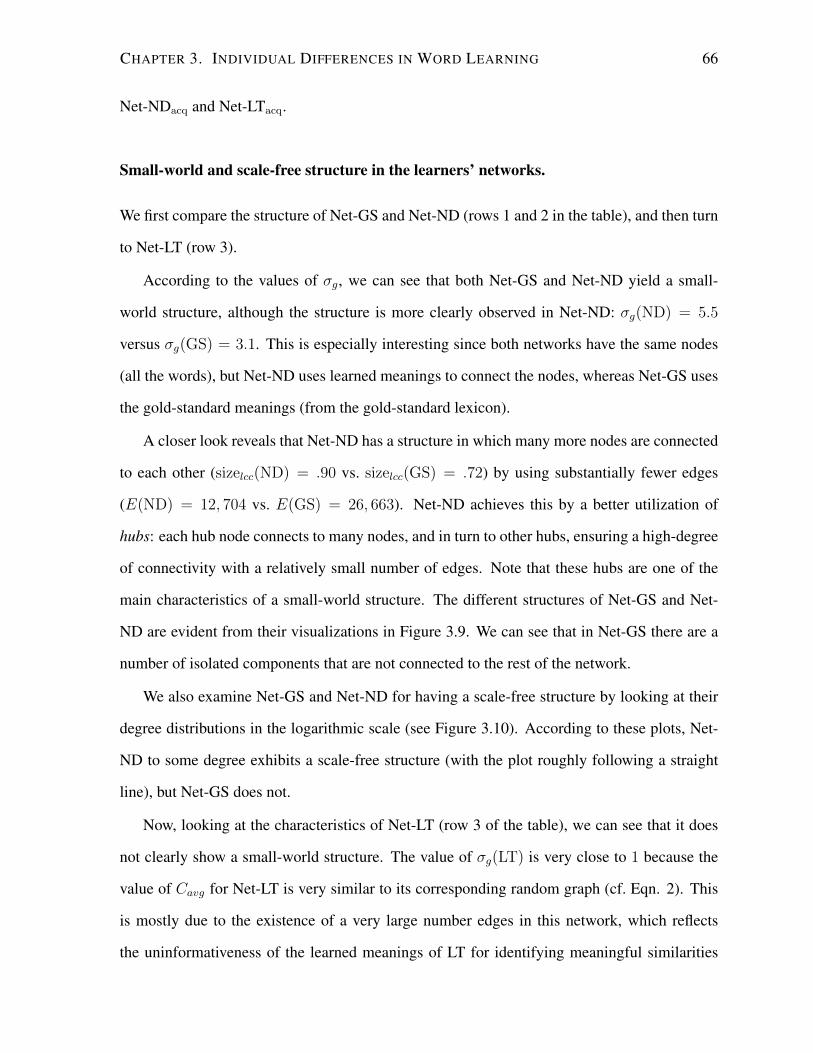
CHAPTER 3. INDIVIDUAL DIFFERENCES IN WORD LEARNING 66
Net-NDacq and Net-LTacq.
Small-world and scale-free structure in the learners’ networks.
We first compare the structure of Net-GS and Net-ND (rows 1 and 2 in the table), and then turn
to Net-LT (row 3).
According to the values of σg, we can see that both Net-GS and Net-ND yield a small-
world structure, although the structure is more clearly observed in Net-ND: σg(ND) = 5.5
versus σg(GS) = 3.1. This is especially interesting since both networks have the same nodes
(all the words), but Net-ND uses learned meanings to connect the nodes, whereas Net-GS uses
the gold-standard meanings (from the gold-standard lexicon).
A closer look reveals that Net-ND has a structure in which many more nodes are connected
to each other (sizelcc(ND) = .90 vs. sizelcc(GS) = .72) by using substantially fewer edges
(E(ND) = 12, 704 vs. E(GS) = 26, 663). Net-ND achieves this by a better utilization of
hubs: each hub node connects to many nodes, and in turn to other hubs, ensuring a high-degree
of connectivity with a relatively small number of edges. Note that these hubs are one of the
main characteristics of a small-world structure. The different structures of Net-GS and Net-
ND are evident from their visualizations in Figure 3.9. We can see that in Net-GS there are a
number of isolated components that are not connected to the rest of the network.
We also examine Net-GS and Net-ND for having a scale-free structure by looking at their
degree distributions in the logarithmic scale (see Figure 3.10). According to these plots, Net-
ND to some degree exhibits a scale-free structure (with the plot roughly following a straight
line), but Net-GS does not.
Now, looking at the characteristics of Net-LT (row 3 of the table), we can see that it does
not clearly show a small-world structure. The value of σg(LT) is very close to 1 because the
value of Cavg for Net-LT is very similar to its corresponding random graph (cf. Eqn. 2). This
is mostly due to the existence of a very large number edges in this network, which reflects
the uninformativeness of the learned meanings of LT for identifying meaningful similarities
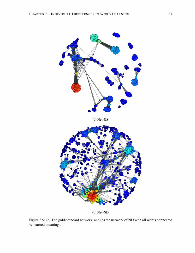
CHAPTER 3. INDIVIDUAL DIFFERENCES IN WORD LEARNING 67
(a) Net-GS
(b) Net-ND
Figure 3.9: (a) The gold-standard network, and (b) the network of ND with all words connectedby learned meanings.
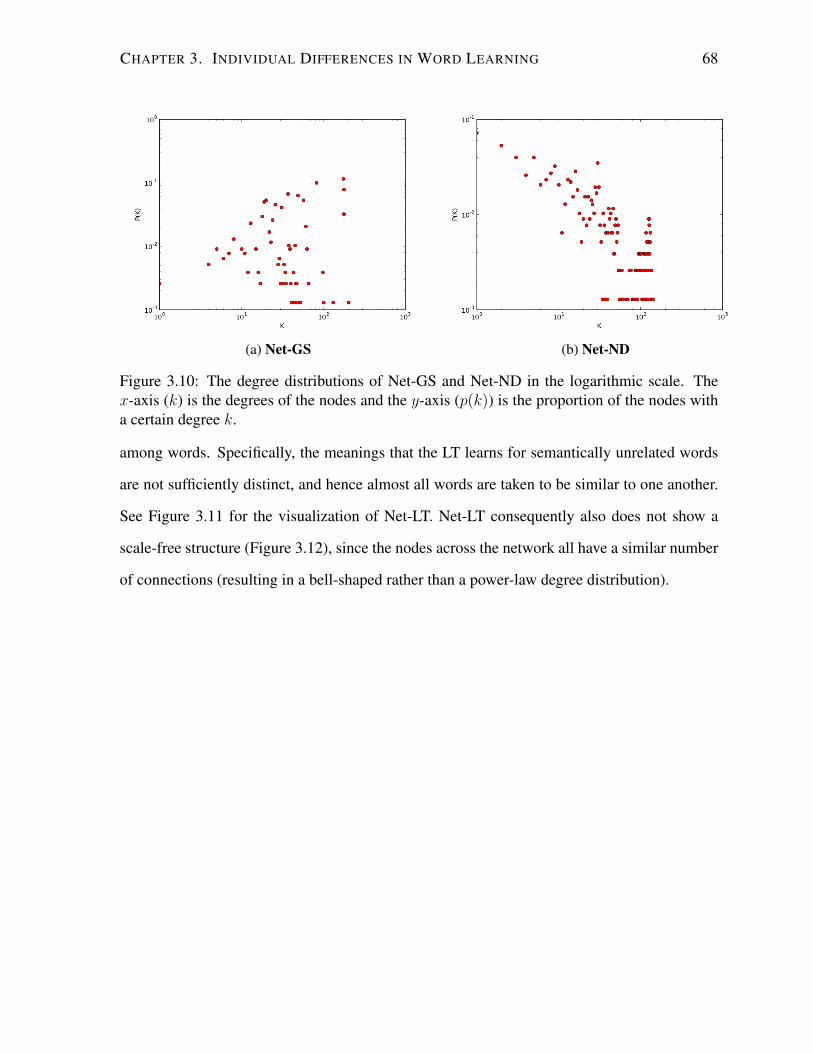
CHAPTER 3. INDIVIDUAL DIFFERENCES IN WORD LEARNING 68
(a) Net-GS (b) Net-ND
Figure 3.10: The degree distributions of Net-GS and Net-ND in the logarithmic scale. Thex-axis (k) is the degrees of the nodes and the y-axis (p(k)) is the proportion of the nodes witha certain degree k.
among words. Specifically, the meanings that the LT learns for semantically unrelated words
are not sufficiently distinct, and hence almost all words are taken to be similar to one another.
See Figure 3.11 for the visualization of Net-LT. Net-LT consequently also does not show a
scale-free structure (Figure 3.12), since the nodes across the network all have a similar number
of connections (resulting in a bell-shaped rather than a power-law degree distribution).
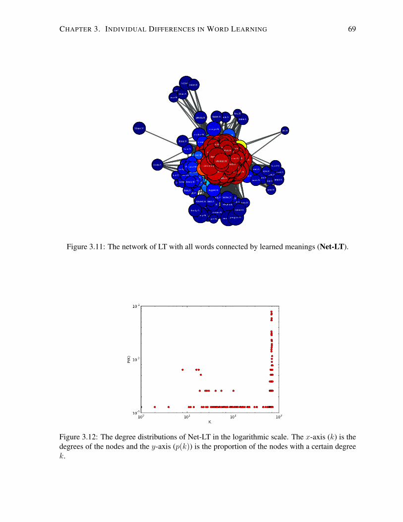
CHAPTER 3. INDIVIDUAL DIFFERENCES IN WORD LEARNING 69
Figure 3.11: The network of LT with all words connected by learned meanings (Net-LT).
Figure 3.12: The degree distributions of Net-LT in the logarithmic scale. The x-axis (k) is thedegrees of the nodes and the y-axis (p(k)) is the proportion of the nodes with a certain degreek.
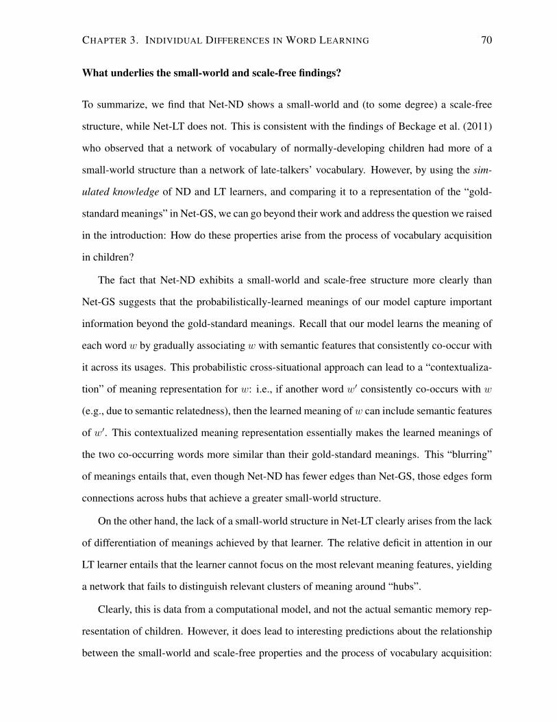
CHAPTER 3. INDIVIDUAL DIFFERENCES IN WORD LEARNING 70
What underlies the small-world and scale-free findings?
To summarize, we find that Net-ND shows a small-world and (to some degree) a scale-free
structure, while Net-LT does not. This is consistent with the findings of Beckage et al. (2011)
who observed that a network of vocabulary of normally-developing children had more of a
small-world structure than a network of late-talkers’ vocabulary. However, by using the sim-
ulated knowledge of ND and LT learners, and comparing it to a representation of the “gold-
standard meanings” in Net-GS, we can go beyond their work and address the question we raised
in the introduction: How do these properties arise from the process of vocabulary acquisition
in children?
The fact that Net-ND exhibits a small-world and scale-free structure more clearly than
Net-GS suggests that the probabilistically-learned meanings of our model capture important
information beyond the gold-standard meanings. Recall that our model learns the meaning of
each word w by gradually associating w with semantic features that consistently co-occur with
it across its usages. This probabilistic cross-situational approach can lead to a “contextualiza-
tion” of meaning representation for w: i.e., if another word w′ consistently co-occurs with w
(e.g., due to semantic relatedness), then the learned meaning ofw can include semantic features
of w′. This contextualized meaning representation essentially makes the learned meanings of
the two co-occurring words more similar than their gold-standard meanings. This “blurring”
of meanings entails that, even though Net-ND has fewer edges than Net-GS, those edges form
connections across hubs that achieve a greater small-world structure.
On the other hand, the lack of a small-world structure in Net-LT clearly arises from the lack
of differentiation of meanings achieved by that learner. The relative deficit in attention in our
LT learner entails that the learner cannot focus on the most relevant meaning features, yielding
a network that fails to distinguish relevant clusters of meaning around “hubs”.
Clearly, this is data from a computational model, and not the actual semantic memory rep-
resentation of children. However, it does lead to interesting predictions about the relationship
between the small-world and scale-free properties and the process of vocabulary acquisition:
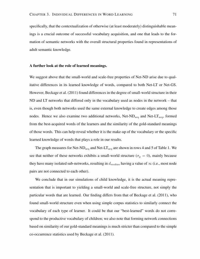
CHAPTER 3. INDIVIDUAL DIFFERENCES IN WORD LEARNING 71
specifically, that the contextualization of otherwise (at least moderately) distinguishable mean-
ings is a crucial outcome of successful vocabulary acquisition, and one that leads to the for-
mation of semantic networks with the overall structural properties found in representations of
adult semantic knowledge.
A further look at the role of learned meanings.
We suggest above that the small-world and scale-free properties of Net-ND arise due to qual-
itative differences in its learned knowledge of words, compared to both Net-LT or Net-GS.
However, Beckage et al. (2011) found differences in the degree of small-world structure in their
ND and LT networks that differed only in the vocabulary used as nodes in the network – that
is, even though both networks used the same external knowledge to create edges among those
nodes. Hence we also examine two additional networks, Net-NDacq and Net-LTacq, formed
from the best-acquired words of the learners and the similarity of the gold-standard meanings
of those words. This can help reveal whether it is the make-up of the vocabulary or the specific
learned knowledge of words that plays a role in our results.
The graph measures for Net-NDacq and Net-LTacq are shown in rows 4 and 5 of Table 1. We
see that neither of these networks exhibits a small-world structure (σg = 0), mainly because
they have many isolated sub-networks, resulting in dmedian having a value of∞ (i.e., most node
pairs are not connected to each other).
We conclude that in our simulations of child knowledge, it is the actual meaning repre-
sentation that is important to yielding a small-world and scale-free structure, not simply the
particular words that are learned. Our finding differs from that of Beckage et al. (2011), who
found small-world structure even when using simple corpus statistics to similarly connect the
vocabulary of each type of learner. It could be that our “best-learned” words do not corre-
spond to the productive vocabulary of children; we also note that forming network connections
based on similarity of our gold-standard meanings is much stricter than compared to the simple
co-occurrence statistics used by Beckage et al. (2011).
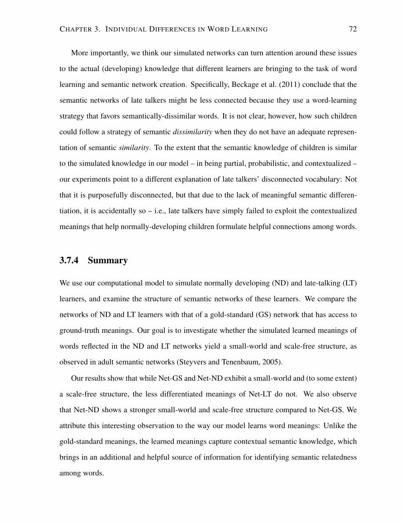
CHAPTER 3. INDIVIDUAL DIFFERENCES IN WORD LEARNING 72
More importantly, we think our simulated networks can turn attention around these issues
to the actual (developing) knowledge that different learners are bringing to the task of word
learning and semantic network creation. Specifically, Beckage et al. (2011) conclude that the
semantic networks of late talkers might be less connected because they use a word-learning
strategy that favors semantically-dissimilar words. It is not clear, however, how such children
could follow a strategy of semantic dissimilarity when they do not have an adequate represen-
tation of semantic similarity. To the extent that the semantic knowledge of children is similar
to the simulated knowledge in our model – in being partial, probabilistic, and contextualized –
our experiments point to a different explanation of late talkers’ disconnected vocabulary: Not
that it is purposefully disconnected, but that due to the lack of meaningful semantic differen-
tiation, it is accidentally so – i.e., late talkers have simply failed to exploit the contextualized
meanings that help normally-developing children formulate helpful connections among words.
3.7.4 Summary
We use our computational model to simulate normally developing (ND) and late-talking (LT)
learners, and examine the structure of semantic networks of these learners. We compare the
networks of ND and LT learners with that of a gold-standard (GS) network that has access to
ground-truth meanings. Our goal is to investigate whether the simulated learned meanings of
words reflected in the ND and LT networks yield a small-world and scale-free structure, as
observed in adult semantic networks (Steyvers and Tenenbaum, 2005).
Our results show that while Net-GS and Net-ND exhibit a small-world and (to some extent)
a scale-free structure, the less differentiated meanings of Net-LT do not. We also observe
that Net-ND shows a stronger small-world and scale-free structure compared to Net-GS. We
attribute this interesting observation to the way our model learns word meanings: Unlike the
gold-standard meanings, the learned meanings capture contextual semantic knowledge, which
brings in an additional and helpful source of information for identifying semantic relatedness
among words.
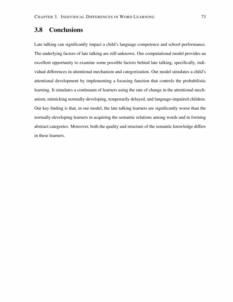
CHAPTER 3. INDIVIDUAL DIFFERENCES IN WORD LEARNING 73
3.8 Conclusions
Late talking can significantly impact a child’s language competence and school performance.
The underlying factors of late talking are still unknown. Our computational model provides an
excellent opportunity to examine some possible factors behind late talking, specifically, indi-
vidual differences in attentional mechanism and categorization. Our model simulates a child’s
attentional development by implementing a focusing function that controls the probabilistic
learning. It simulates a continuum of learners using the rate of change in the attentional mech-
anism, mimicking normally-developing, temporarily delayed, and language-impaired children.
Our key finding is that, in our model, the late talking learners are significantly worse than the
normally-developing learners in acquiring the semantic relations among words and in forming
abstract categories. Moreover, both the quality and structure of the semantic knowledge differs
in these learners.
Chapter 4
Memory, Attention, and Word Learning
While computational modeling has been critical in giving precise accounts of the possible pro-
cesses and influences involved in word learning (e.g., Siskind, 1996; Regier, 2005; Yu, 2005;
Fazly et al., 2010b), such models have generally not given sufficient attention to the broader
interactions of language acquisition with other aspects of cognition and cognitive development.
Here we extend our computational model of word learning to incorporate a forgetting and at-
tentional mechanism. We show that this model accounts for experimental results on children
as well as several patterns observed in adults. In Section 4.1, I explain the relevant related
work. Section 4.2 provides a detailed explanation of the extensions to the model. The remain-
ing sections (Section 4.3 to Section 4.5) discuss our experiments and findings on modeling two
important phenomena (the “spacing effect” and “desirable difficulty” in learning) that demon-
strate the interaction of word learning and other cognitive processes. The work presented in
Section 4.2 and Section 4.3 is published in Nematzadeh et al. (2012a). Section 4.4 and Sec-
tion 4.5 are published in Nematzadeh et al. (2013b).
4.1 Related Work
Memory limitations and attentional mechanisms are of particular interest here, with recent
computational studies reconfirming their important role in aspects of word learning. For exam-
74
CHAPTER 4. MEMORY, ATTENTION, AND WORD LEARNING 75
ple, Frank et al. (2010) show that memory limitations are key to matching human performance
in a model of word segmentation, while Smith et al. (2010) further demonstrate how attention
plays a role in word learning by forming the basis for abstracting over the input. But much
potential remains for computational modeling to contribute to a better understanding of the
role of memory and attention in word learning.
One area where there is much experimental evidence relevant to these interactions is in the
investigation of the spacing effect in learning (Ebbinghaus, 1885; Glenberg, 1979; Dempster,
1996; Cepeda et al., 2006). The observation is that people generally show better learning when
the presentations of the target items to be learned are “spaced” — i.e., distributed over a period
of time — instead of being “massed” — i.e., presented together one after the other. Investiga-
tions of the spacing effect often use a word learning task as the target learning event, and such
studies have looked at the performance of adults as well as children (Glenberg, 1976; Pavlik
and Anderson, 2005; Vlach et al., 2008). While this work involves controlled laboratory condi-
tions, the spacing effect is very robust across domains and tasks (Dempster, 1989), suggesting
that the underlying cognitive processes likely play a role in natural conditions of word learning
as well.
Hypothesized explanations for the spacing effect have included both memory limitations
and attention. For example, many researchers assume that the process of forgetting is responsi-
ble for the improved performance in the spaced presentation: Because participants forget more
of what they have learned in the longer interval, they learn more from subsequent presentations
(Melton, 1967; Jacoby, 1978; Cuddy and Jacoby, 1982). However, the precise relation be-
tween forgetting and improved learning has not been made clear. It has also been proposed that
subjects attend more to items in the spaced presentation because accessing less recent (more
novel) items in memory requires more effort or attention (Hintzman, 1974). However, the pre-
cise attentional mechanism at work in the spacing experiments is not completely understood.
While such proposals have been discussed for many years, to our knowledge, there is as
yet no detailed computational model of the precise manner in which forgetting and attention to
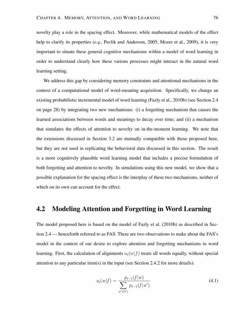
CHAPTER 4. MEMORY, ATTENTION, AND WORD LEARNING 76
novelty play a role in the spacing effect. Moreover, while mathematical models of the effect
help to clarify its properties (e.g., Pavlik and Anderson, 2005; Mozer et al., 2009), it is very
important to situate these general cognitive mechanisms within a model of word learning in
order to understand clearly how these various processes might interact in the natural word
learning setting.
We address this gap by considering memory constraints and attentional mechanisms in the
context of a computational model of word-meaning acquisition. Specifically, we change an
existing probabilistic incremental model of word learning (Fazly et al., 2010b) (see Section 2.4
on page 28) by integrating two new mechanisms: (i) a forgetting mechanism that causes the
learned associations between words and meanings to decay over time; and (ii) a mechanism
that simulates the effects of attention to novelty on in-the-moment learning. We note that
the extensions discussed in Section 3.2 are mutually compatible with those proposed here,
but they are not used in replicating the behavioral data discussed in this section. The result
is a more cognitively plausible word learning model that includes a precise formulation of
both forgetting and attention to novelty. In simulations using this new model, we show that a
possible explanation for the spacing effect is the interplay of these two mechanisms, neither of
which on its own can account for the effect.
4.2 Modeling Attention and Forgetting in Word Learning
The model proposed here is based on the model of Fazly et al. (2010b) as described in Sec-
tion 2.4 — henceforth referred to as FAS. There are two observations to make about the FAS’s
model in the context of our desire to explore attention and forgetting mechanisms in word
learning. First, the calculation of alignments at(w|f) treats all words equally, without special
attention to any particular item(s) in the input (see Section 2.4.2 for more details):
at(w |f ) =pt−1(f |w)∑
w ′∈Ut
pt−1(f |w ′)(4.1)
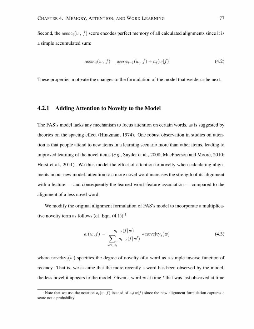
CHAPTER 4. MEMORY, ATTENTION, AND WORD LEARNING 77
Second, the assoct(w, f) score encodes perfect memory of all calculated alignments since it is
a simple accumulated sum:
assoct(w, f) = assoct−1(w, f) + at(w|f) (4.2)
These properties motivate the changes to the formulation of the model that we describe next.
4.2.1 Adding Attention to Novelty to the Model
The FAS’s model lacks any mechanism to focus attention on certain words, as is suggested by
theories on the spacing effect (Hintzman, 1974). One robust observation in studies on atten-
tion is that people attend to new items in a learning scenario more than other items, leading to
improved learning of the novel items (e.g., Snyder et al., 2008; MacPherson and Moore, 2010;
Horst et al., 2011). We thus model the effect of attention to novelty when calculating align-
ments in our new model: attention to a more novel word increases the strength of its alignment
with a feature — and consequently the learned word–feature association — compared to the
alignment of a less novel word.
We modify the original alignment formulation of FAS’s model to incorporate a multiplica-
tive novelty term as follows (cf. Eqn. (4.1)):1
at(w , f ) =pt−1 (f |w)∑
w ′∈Ut
pt−1 (f |w ′)∗ noveltyt(w) (4.3)
where noveltyt(w) specifies the degree of novelty of a word as a simple inverse function of
recency. That is, we assume that the more recently a word has been observed by the model,
the less novel it appears to the model. Given a word w at time t that was last observed at time
1Note that we use the notation at(w, f) instead of at(w|f) since the new alignment formulation captures ascore not a probability.
CHAPTER 4. MEMORY, ATTENTION, AND WORD LEARNING 78
tlastw , we calculate noveltyt(w) as:
noveltyt(w) = 1− recency(t, tlastw) (4.4)
where recency(t, tlastw) is inversely proportional to the difference between t and tlastw :
recency(t, tlastw) =1
(t− tlastw+1)δ(4.5)
where δ is a parameter that controls the growth rate of recency. We set novelty(w) to be 1 for
the first exposure of the word.
4.2.2 Adding a Forgetting Mechanism to the Model
Given the observation above that assoct(w, f) embeds perfect memory in the FAS’s model, we
add a forgetting mechanism by reformulating assoct(w, f) to incorporate a decay over time
of the component alignments at(w|f). In order to take a cognitively plausible approach to
calculating this function, we observe that assoct(w, f) in the FAS’s model serves a similar
function to activation in the ACT-R model of memory (Anderson and Lebiere, 1998). In ACT-
R, activation of an item is the sum of individual memory strengthenings for that item, just as
assoct(w, f) is a sum of individual alignment strengths for the pair (w, f). A crucial difference
is that memory strengthenings in ACT-R undergo decay. Specifically, activation of an item m
at time t is calculated as: actt(m) = ln(∑
t′∈τ 1/(t − t′)d), where τ is a set consisting of the
time of each presentation of m, and d is a constant decay parameter.
We adapt this formulation for assoct(w, f) with the following changes: First, in the act
formula, the constant 1 in the numerator is the basic strength of each presentation to memory.
In our model, this is not a constant but rather the strength of alignment, at(w|f). Second,
since the strength of presentations is not constant, we vary the rate of decay depending on the
strength of a presentation: We assume that stronger alignments should be more entrenched in
memory and thus decay more slowly than weaker alignments. Thus, each alignment undergoes
CHAPTER 4. MEMORY, ATTENTION, AND WORD LEARNING 79
a decay which is dependent on the strength of the alignment rather than a constant decay d. We
thus define assoct(w, f) to be:
assoct(f, w) = ln
(t∑
t′=1
at′(w|f)
(t− t′)dat′
)(4.6)
where the decay for each alignment dat′ is:
dat′ =d
at′(w|f)(4.7)
where d is a constant parameter. Note that dat′ decreases as at′(w|f) increases.
4.3 Experiments on Spacing Effect
The input data consists of a set of utterances paired with their corresponding scene represen-
tations and is the same as the data explained in Section 3.5.1: The utterances are taken from
the CHILDES corpus (MacWhinney, 2000), and their corresponding scene representations are
generated using the input-generation lexicon of Nematzadeh et al. (2012b) (see Section 3.5.1).
The input-generation lexicon contains the gold-standard meaning (gs(w)) of all the words (w)
in our corpus. The gold-standard meaning is a vector of semantic features and their assigned
scores (Figure 3.6 on page 52).
First, we examine the overall word learning behaviour in our new model. Then we look
at spacing effects in the learning of novel words. In both these experiments, we compare the
behavior of our model with the model of FAS to clearly illustrate the effects of forgetting and
attention to novelty in the new model. Next we turn to further experiments exploring in more
detail the interaction of forgetting and attention to novelty in producing spacing effects.
CHAPTER 4. MEMORY, ATTENTION, AND WORD LEARNING 80
4.3.1 Experiment 1: Word Learning over Time
Generally, the model of FAS has increasing comprehension of words as it is exposed to more
input over time. In our model, we expect attention to novelty to facilitate word learning, by
focusing more on newly observed words, whereas forgetting is expected to hinder learning. We
need to see if the new model is able to learn words effectively when subject to the combined
effects of these two influences.
As in Section 3.3.1, to measure how well a word w is learned in each model, we compare
its learned meaning l(w) (a vector holding the values of the meaning probability p(·|w)) to its
gold-standard meaning gs(w):
acq(w) = sim(l(w), gs(w)) (4.8)
where sim is the cosine similarity between the two meaning vectors, gs(w) and l(w). The
better the model learns the meaning of w, the closer l(w) would be to gs(w), and the higher
the value of sim would become. To evaluate the overall behaviour of a model, at each point in
time, we average the acq score of all the words that the model has seen.
We train each model – FAS’s and the extended model – on 10, 000 input utterance–scene
pairs and compare their patterns of word learning over time (Figure 4.1).2 We can see that in
the original model, the average acq score is mostly increasing over time before leveling off.
Our new model starts at a higher average acq score compared to FAS’s model, since the effect
of attention to novelty is stronger than the effect of forgetting in early stages of training. There
is a sharp decrease in the acq scores after the early training stage, which then levels off. The
early decrease in acq scores occurs because many of the words the model is exposed to early
on are not learned very well initially, and so forgetting occurs at a higher rate during that stage.
The model subsequently stabilizes, and the acq scores level off although at a lower absolute
2The constant decay parameter d in Eqn. (4.7) is set to 0.03 in this experiment. The growth rate δ in calculatingrecency (Eqn. (4.5)) is set to 0.25 in all experiments discussed in this section. These parameters are set ondevelopment data.
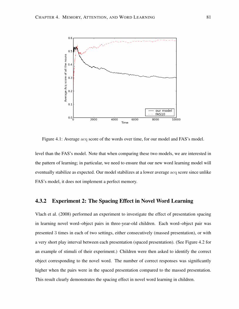
CHAPTER 4. MEMORY, ATTENTION, AND WORD LEARNING 81
Figure 4.1: Average acq score of the words over time, for our model and FAS’s model.
level than the FAS’s model. Note that when comparing these two models, we are interested in
the pattern of learning; in particular, we need to ensure that our new word learning model will
eventually stabilize as expected. Our model stabilizes at a lower average acq score since unlike
FAS’s model, it does not implement a perfect memory.
4.3.2 Experiment 2: The Spacing Effect in Novel Word Learning
Vlach et al. (2008) performed an experiment to investigate the effect of presentation spacing
in learning novel word–object pairs in three-year-old children. Each word–object pair was
presented 3 times in each of two settings, either consecutively (massed presentation), or with
a very short play interval between each presentation (spaced presentation). (See Figure 4.2 for
an example of stimuli of their experiment.) Children were then asked to identify the correct
object corresponding to the novel word. The number of correct responses was significantly
higher when the pairs were in the spaced presentation compared to the massed presentation.
This result clearly demonstrates the spacing effect in novel word learning in children.
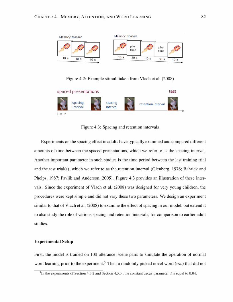
CHAPTER 4. MEMORY, ATTENTION, AND WORD LEARNING 82
Figure 4.2: Example stimuli taken from Vlach et al. (2008)
Figure 4.3: Spacing and retention intervals
Experiments on the spacing effect in adults have typically examined and compared different
amounts of time between the spaced presentations, which we refer to as the spacing interval.
Another important parameter in such studies is the time period between the last training trial
and the test trial(s), which we refer to as the retention interval (Glenberg, 1976; Bahrick and
Phelps, 1987; Pavlik and Anderson, 2005). Figure 4.3 provides an illustration of these inter-
vals. Since the experiment of Vlach et al. (2008) was designed for very young children, the
procedures were kept simple and did not vary these two parameters. We design an experiment
similar to that of Vlach et al. (2008) to examine the effect of spacing in our model, but extend it
to also study the role of various spacing and retention intervals, for comparison to earlier adult
studies.
Experimental Setup
First, the model is trained on 100 utterance–scene pairs to simulate the operation of normal
word learning prior to the experiment.3 Then a randomly picked novel word (nw) that did not
3In the experiments of Section 4.3.2 and Section 4.3.3 , the constant decay parameter d is equal to 0.04.
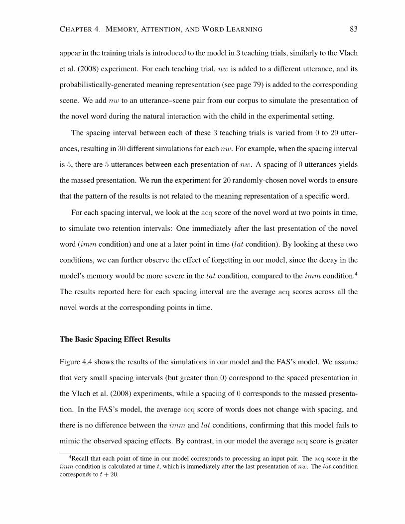
CHAPTER 4. MEMORY, ATTENTION, AND WORD LEARNING 83
appear in the training trials is introduced to the model in 3 teaching trials, similarly to the Vlach
et al. (2008) experiment. For each teaching trial, nw is added to a different utterance, and its
probabilistically-generated meaning representation (see page 79) is added to the corresponding
scene. We add nw to an utterance–scene pair from our corpus to simulate the presentation of
the novel word during the natural interaction with the child in the experimental setting.
The spacing interval between each of these 3 teaching trials is varied from 0 to 29 utter-
ances, resulting in 30 different simulations for each nw. For example, when the spacing interval
is 5, there are 5 utterances between each presentation of nw. A spacing of 0 utterances yields
the massed presentation. We run the experiment for 20 randomly-chosen novel words to ensure
that the pattern of the results is not related to the meaning representation of a specific word.
For each spacing interval, we look at the acq score of the novel word at two points in time,
to simulate two retention intervals: One immediately after the last presentation of the novel
word (imm condition) and one at a later point in time (lat condition). By looking at these two
conditions, we can further observe the effect of forgetting in our model, since the decay in the
model’s memory would be more severe in the lat condition, compared to the imm condition.4
The results reported here for each spacing interval are the average acq scores across all the
novel words at the corresponding points in time.
The Basic Spacing Effect Results
Figure 4.4 shows the results of the simulations in our model and the FAS’s model. We assume
that very small spacing intervals (but greater than 0) correspond to the spaced presentation in
the Vlach et al. (2008) experiments, while a spacing of 0 corresponds to the massed presenta-
tion. In the FAS’s model, the average acq score of words does not change with spacing, and
there is no difference between the imm and lat conditions, confirming that this model fails to
mimic the observed spacing effects. By contrast, in our model the average acq score is greater
4Recall that each point of time in our model corresponds to processing an input pair. The acq score in theimm condition is calculated at time t, which is immediately after the last presentation of nw. The lat conditioncorresponds to t+ 20.
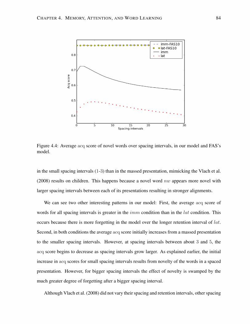
CHAPTER 4. MEMORY, ATTENTION, AND WORD LEARNING 84
Figure 4.4: Average acq score of novel words over spacing intervals, in our model and FAS’smodel.
in the small spacing intervals (1-3) than in the massed presentation, mimicking the Vlach et al.
(2008) results on children. This happens because a novel word nw appears more novel with
larger spacing intervals between each of its presentations resulting in stronger alignments.
We can see two other interesting patterns in our model: First, the average acq score of
words for all spacing intervals is greater in the imm condition than in the lat condition. This
occurs because there is more forgetting in the model over the longer retention interval of lat.
Second, in both conditions the average acq score initially increases from a massed presentation
to the smaller spacing intervals. However, at spacing intervals between about 3 and 5, the
acq score begins to decrease as spacing intervals grow larger. As explained earlier, the initial
increase in acq scores for small spacing intervals results from novelty of the words in a spaced
presentation. However, for bigger spacing intervals the effect of novelty is swamped by the
much greater degree of forgetting after a bigger spacing interval.
Although Vlach et al. (2008) did not vary their spacing and retention intervals, other spacing
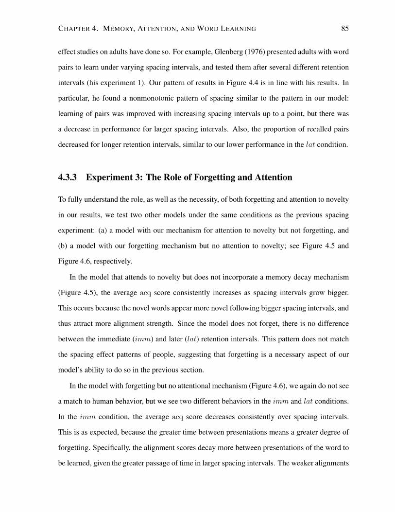
CHAPTER 4. MEMORY, ATTENTION, AND WORD LEARNING 85
effect studies on adults have done so. For example, Glenberg (1976) presented adults with word
pairs to learn under varying spacing intervals, and tested them after several different retention
intervals (his experiment 1). Our pattern of results in Figure 4.4 is in line with his results. In
particular, he found a nonmonotonic pattern of spacing similar to the pattern in our model:
learning of pairs was improved with increasing spacing intervals up to a point, but there was
a decrease in performance for larger spacing intervals. Also, the proportion of recalled pairs
decreased for longer retention intervals, similar to our lower performance in the lat condition.
4.3.3 Experiment 3: The Role of Forgetting and Attention
To fully understand the role, as well as the necessity, of both forgetting and attention to novelty
in our results, we test two other models under the same conditions as the previous spacing
experiment: (a) a model with our mechanism for attention to novelty but not forgetting, and
(b) a model with our forgetting mechanism but no attention to novelty; see Figure 4.5 and
Figure 4.6, respectively.
In the model that attends to novelty but does not incorporate a memory decay mechanism
(Figure 4.5), the average acq score consistently increases as spacing intervals grow bigger.
This occurs because the novel words appear more novel following bigger spacing intervals, and
thus attract more alignment strength. Since the model does not forget, there is no difference
between the immediate (imm) and later (lat) retention intervals. This pattern does not match
the spacing effect patterns of people, suggesting that forgetting is a necessary aspect of our
model’s ability to do so in the previous section.
In the model with forgetting but no attentional mechanism (Figure 4.6), we again do not see
a match to human behavior, but we see two different behaviors in the imm and lat conditions.
In the imm condition, the average acq score decreases consistently over spacing intervals.
This is as expected, because the greater time between presentations means a greater degree of
forgetting. Specifically, the alignment scores decay more between presentations of the word to
be learned, given the greater passage of time in larger spacing intervals. The weaker alignments
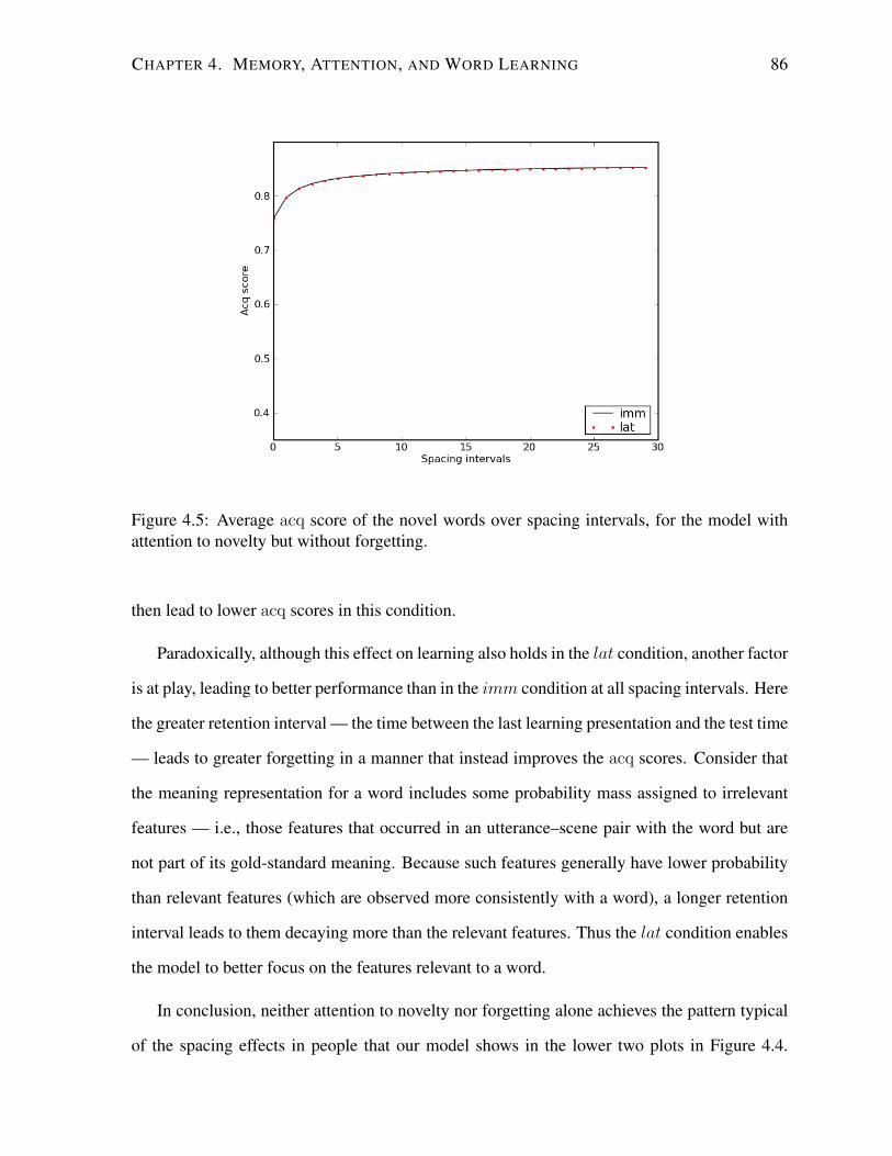
CHAPTER 4. MEMORY, ATTENTION, AND WORD LEARNING 86
Figure 4.5: Average acq score of the novel words over spacing intervals, for the model withattention to novelty but without forgetting.
then lead to lower acq scores in this condition.
Paradoxically, although this effect on learning also holds in the lat condition, another factor
is at play, leading to better performance than in the imm condition at all spacing intervals. Here
the greater retention interval — the time between the last learning presentation and the test time
— leads to greater forgetting in a manner that instead improves the acq scores. Consider that
the meaning representation for a word includes some probability mass assigned to irrelevant
features — i.e., those features that occurred in an utterance–scene pair with the word but are
not part of its gold-standard meaning. Because such features generally have lower probability
than relevant features (which are observed more consistently with a word), a longer retention
interval leads to them decaying more than the relevant features. Thus the lat condition enables
the model to better focus on the features relevant to a word.
In conclusion, neither attention to novelty nor forgetting alone achieves the pattern typical
of the spacing effects in people that our model shows in the lower two plots in Figure 4.4.
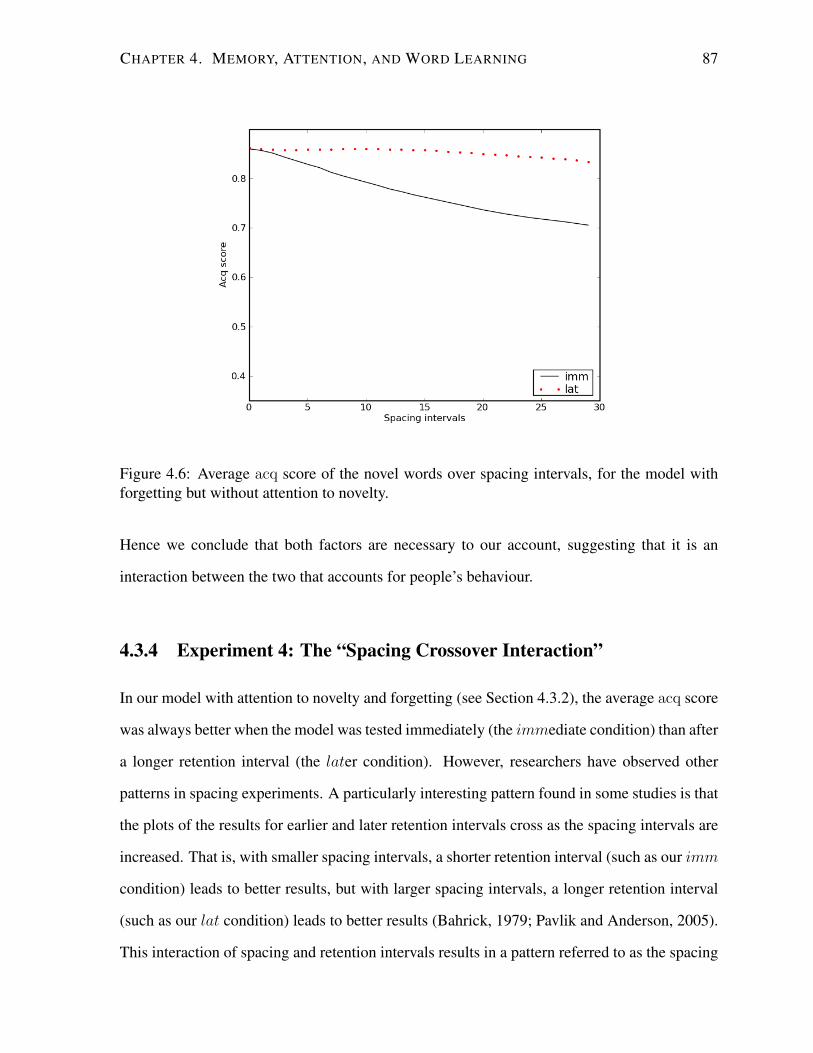
CHAPTER 4. MEMORY, ATTENTION, AND WORD LEARNING 87
Figure 4.6: Average acq score of the novel words over spacing intervals, for the model withforgetting but without attention to novelty.
Hence we conclude that both factors are necessary to our account, suggesting that it is an
interaction between the two that accounts for people’s behaviour.
4.3.4 Experiment 4: The “Spacing Crossover Interaction”
In our model with attention to novelty and forgetting (see Section 4.3.2), the average acq score
was always better when the model was tested immediately (the immediate condition) than after
a longer retention interval (the later condition). However, researchers have observed other
patterns in spacing experiments. A particularly interesting pattern found in some studies is that
the plots of the results for earlier and later retention intervals cross as the spacing intervals are
increased. That is, with smaller spacing intervals, a shorter retention interval (such as our imm
condition) leads to better results, but with larger spacing intervals, a longer retention interval
(such as our lat condition) leads to better results (Bahrick, 1979; Pavlik and Anderson, 2005).
This interaction of spacing and retention intervals results in a pattern referred to as the spacing
CHAPTER 4. MEMORY, ATTENTION, AND WORD LEARNING 88
crossover interaction (Pavlik and Anderson, 2005). This pattern is different from the Glenberg
(1976) experiment and from the pattern of results shown earlier for our model (Figure 4.4).
We looked at an experiment in which the spacing crossover pattern was observed: Pavlik
and Anderson (2005) taught Japanese–English word pairs to subjects, varying the spacing and
retention intervals. One difference we noticed between the experiment of Pavlik and Anderson
(2005) and Glenberg (1976) is that in the former, the presentation period of the stimulus was
5 seconds, whereas in the latter, it was 3 seconds. We hypothesize that the difference between
the amount of time for the presentation periods might explain the different spacing patterns in
these experiments.
We currently cannot model presentation time directly in our model, since having access to
an input longer does not change its computation of alignments between words and features.
However, we can indirectly model a difference in presentation time by modifying the amount
of memory decay: We assume that when an item is presented longer, it is learned better and
therefore subject to less forgetting. We run the spacing experiment with a smaller forgetting
parameter to model the longer presentation period used in Pavlik and Anderson (2005) versus
Glenberg (1976).5
Our results using the decreased level of forgetting, given in Figure 4.7, show the expected
crossover interaction between the retention and spacing intervals: for smaller spacing intervals,
the acq scores are better in the imm condition, whereas for larger spacing intervals, they are
better in the lat condition. Thus, our model suggests an explanation for the observed crossover:
in tasks which strengthen the learning of the target item — and thus lessen the effect of forget-
ting — we expect to see a benefit of later retention trials in experiments with people.
4.3.5 Summary
The spacing effect (where people learn items better when multiple presentations are spread over
time) has been studied extensively and is found to be robust over different types of tasks and
5Here, the decay parameter is set to 0.03.
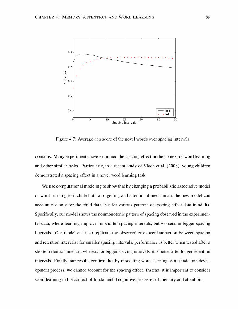
CHAPTER 4. MEMORY, ATTENTION, AND WORD LEARNING 89
Figure 4.7: Average acq score of the novel words over spacing intervals
domains. Many experiments have examined the spacing effect in the context of word learning
and other similar tasks. Particularly, in a recent study of Vlach et al. (2008), young children
demonstrated a spacing effect in a novel word learning task.
We use computational modeling to show that by changing a probabilistic associative model
of word learning to include both a forgetting and attentional mechanism, the new model can
account not only for the child data, but for various patterns of spacing effect data in adults.
Specifically, our model shows the nonmonotonic pattern of spacing observed in the experimen-
tal data, where learning improves in shorter spacing intervals, but worsens in bigger spacing
intervals. Our model can also replicate the observed crossover interaction between spacing
and retention intervals: for smaller spacing intervals, performance is better when tested after a
shorter retention interval, whereas for bigger spacing intervals, it is better after longer retention
intervals. Finally, our results confirm that by modelling word learning as a standalone devel-
opment process, we cannot account for the spacing effect. Instead, it is important to consider
word learning in the context of fundamental cognitive processes of memory and attention.
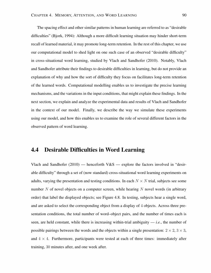
CHAPTER 4. MEMORY, ATTENTION, AND WORD LEARNING 90
The spacing effect and other similar patterns in human learning are referred to as “desirable
difficulties” (Bjork, 1994): Although a more difficult learning situation may hinder short-term
recall of learned material, it may promote long-term retention. In the rest of this chapter, we use
our computational model to shed light on one such case of an observed “desirable difficulty”
in cross-situational word learning, studied by Vlach and Sandhofer (2010). Notably, Vlach
and Sandhofer attribute their findings to desirable difficulties in learning, but do not provide an
explanation of why and how the sort of difficulty they focus on facilitates long-term retention
of the learned words. Computational modelling enables us to investigate the precise learning
mechanisms, and the variations in the input conditions, that might explain these findings. In the
next section, we explain and analyze the experimental data and results of Vlach and Sandhofer
in the context of our model. Finally, we describe the way we simulate these experiments
using our model, and how this enables us to examine the role of several different factors in the
observed pattern of word learning.
4.4 Desirable Difficulties in Word Learning
Vlach and Sandhofer (2010) — henceforth V&S — explore the factors involved in “desir-
able difficulty” through a set of (now standard) cross-situational word learning experiments on
adults, varying the presentation and testing conditions. In each N ×N trial, subjects see some
number N of novel objects on a computer screen, while hearing N novel words (in arbitrary
order) that label the displayed objects; see Figure 4.8. In testing, subjects hear a single word,
and are asked to select the corresponding object from a display of 4 objects. Across three pre-
sentation conditions, the total number of word–object pairs, and the number of times each is
seen, are held constant, while there is increasing within-trial ambiguity — i.e., the number of
possible pairings between the words and the objects within a single presentation: 2× 2, 3× 3,
and 4 × 4. Furthermore, participants were tested at each of three times: immediately after
training, 30 minutes after, and one week after.
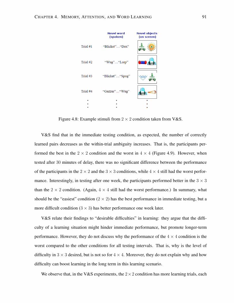
CHAPTER 4. MEMORY, ATTENTION, AND WORD LEARNING 91
Figure 4.8: Example stimuli from 2× 2 condition taken from V&S.
V&S find that in the immediate testing condition, as expected, the number of correctly
learned pairs decreases as the within-trial ambiguity increases. That is, the participants per-
formed the best in the 2 × 2 condition and the worst in 4 × 4 (Figure 4.9). However, when
tested after 30 minutes of delay, there was no significant difference between the performance
of the participants in the 2× 2 and the 3× 3 conditions, while 4× 4 still had the worst perfor-
mance. Interestingly, in testing after one week, the participants performed better in the 3 × 3
than the 2 × 2 condition. (Again, 4 × 4 still had the worst performance.) In summary, what
should be the “easiest” condition (2 × 2) has the best performance in immediate testing, but a
more difficult condition (3× 3) has better performance one week later.
V&S relate their findings to “desirable difficulties” in learning: they argue that the diffi-
culty of a learning situation might hinder immediate performance, but promote longer-term
performance. However, they do not discuss why the performance of the 4× 4 condition is the
worst compared to the other conditions for all testing intervals. That is, why is the level of
difficulty in 3× 3 desired, but is not so for 4× 4. Moreover, they do not explain why and how
difficulty can boost learning in the long term in this learning scenario.
We observe that, in the V&S experiments, the 2×2 condition has more learning trials, each
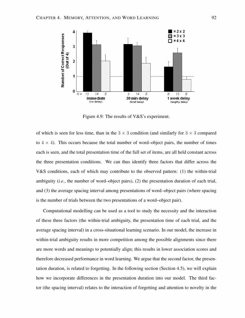
CHAPTER 4. MEMORY, ATTENTION, AND WORD LEARNING 92
Figure 4.9: The results of V&S’s experiment.
of which is seen for less time, than in the 3 × 3 condition (and similarly for 3 × 3 compared
to 4 × 4). This occurs because the total number of word–object pairs, the number of times
each is seen, and the total presentation time of the full set of items, are all held constant across
the three presentation conditions. We can thus identify three factors that differ across the
V&S conditions, each of which may contribute to the observed pattern: (1) the within-trial
ambiguity (i.e., the number of word–object pairs), (2) the presentation duration of each trial,
and (3) the average spacing interval among presentations of word–object pairs (where spacing
is the number of trials between the two presentations of a word–object pair).
Computational modelling can be used as a tool to study the necessity and the interaction
of these three factors (the within-trial ambiguity, the presentation time of each trial, and the
average spacing interval) in a cross-situational learning scenario. In our model, the increase in
within-trial ambiguity results in more competition among the possible alignments since there
are more words and meanings to potentially align; this results in lower association scores and
therefore decreased performance in word learning. We argue that the second factor, the presen-
tation duration, is related to forgetting. In the following section (Section 4.5), we will explain
how we incorporate differences in the presentation duration into our model. The third fac-
tor (the spacing interval) relates to the interaction of forgetting and attention to novelty in the
CHAPTER 4. MEMORY, ATTENTION, AND WORD LEARNING 93
model: As the spacing interval becomes larger, the amount of forgetting increases, resulting in
lower association scores between words and features; however, the novelty of words and con-
sequently their association scores increases as the spacing interval gets larger. Thus, varying
the spacing interval affects the performance of the model (see Section 4.3.2 for more details).
We use our model to study the interaction of these three factors, with the goal of providing
a more precise explanation for the desirable difficulty observed in the experiments of V&S.
Next, we explain our methodology, including our input generation, and the simulation of the
V&S experiments.
4.5 Experiments on Desirable Difficulties
4.5.1 Methodology
Input Generation
To generate the input stimuli for our model, we need to pair words with a meaning representa-
tion that corresponds to the depiction of the corresponding object in the experimental situation
of Figure 4.8. To do so, we draw on the input-generation lexicon explained in Section 3.5.1,
which was previously used to automatically annotate corpora of child-directed utterances with
meaning features corresponding to the words in those utterances. Here, we use the lexicon
to provide a source of naturalistic meaning representations (“novel object descriptions”) for a
set of “novel” words (i.e., the words in the input stimuli are unknown to the model, as in the
experiments we are modeling).
When a word is used in an input trial, its meaning features are probabilistically sampled
from its gold-standard meaning (gs(w), see Section 4.3 on page 79) according to the weight of
each feature in the lexical entry of the word. This probabilistic sampling captures our intuition
that a participant, when faced with a trial in the cross-situational experiment of Figure 4.8, will
grasp some features of the novel objects but not necessarily all. Each trial of the input is then
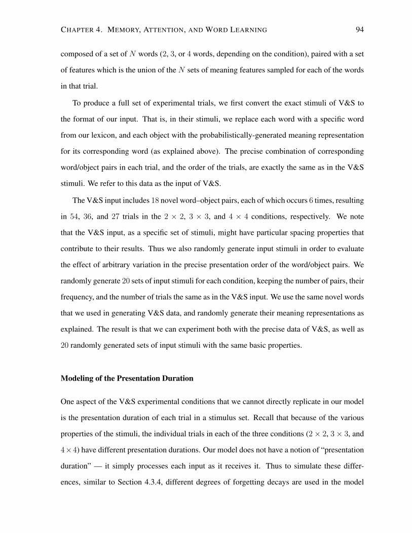
CHAPTER 4. MEMORY, ATTENTION, AND WORD LEARNING 94
composed of a set of N words (2, 3, or 4 words, depending on the condition), paired with a set
of features which is the union of the N sets of meaning features sampled for each of the words
in that trial.
To produce a full set of experimental trials, we first convert the exact stimuli of V&S to
the format of our input. That is, in their stimuli, we replace each word with a specific word
from our lexicon, and each object with the probabilistically-generated meaning representation
for its corresponding word (as explained above). The precise combination of corresponding
word/object pairs in each trial, and the order of the trials, are exactly the same as in the V&S
stimuli. We refer to this data as the input of V&S.
The V&S input includes 18 novel word–object pairs, each of which occurs 6 times, resulting
in 54, 36, and 27 trials in the 2 × 2, 3 × 3, and 4 × 4 conditions, respectively. We note
that the V&S input, as a specific set of stimuli, might have particular spacing properties that
contribute to their results. Thus we also randomly generate input stimuli in order to evaluate
the effect of arbitrary variation in the precise presentation order of the word/object pairs. We
randomly generate 20 sets of input stimuli for each condition, keeping the number of pairs, their
frequency, and the number of trials the same as in the V&S input. We use the same novel words
that we used in generating V&S data, and randomly generate their meaning representations as
explained. The result is that we can experiment both with the precise data of V&S, as well as
20 randomly generated sets of input stimuli with the same basic properties.
Modeling of the Presentation Duration
One aspect of the V&S experimental conditions that we cannot directly replicate in our model
is the presentation duration of each trial in a stimulus set. Recall that because of the various
properties of the stimuli, the individual trials in each of the three conditions (2× 2, 3× 3, and
4×4) have different presentation durations. Our model does not have a notion of “presentation
duration” — it simply processes each input as it receives it. Thus to simulate these differ-
ences, similar to Section 4.3.4, different degrees of forgetting decays are used in the model

CHAPTER 4. MEMORY, ATTENTION, AND WORD LEARNING 95
(see Eqn. (4.7)). The intuition is that subjects forget faster in a condition with a shorter pre-
sentation duration, since they have less time to absorb the stimuli in each trial. The forgetting
decay is thus set to a larger value in the 2 × 2 condition (where the presentation time is the
smallest), and successively smaller in each of the 3× 3 and 4× 4 conditions.6
Simulation of the V&S Experiments
We train our model by presenting the set of inputs for a given condition, where it learns in-
crementally in response to each trial. Similarly to V&S, we evaluate our model at three points
of time after training: immediately after processing the last input (time = t), at t + 30, and at
t + 350. These times were chosen to loosely reflect the three time intervals in V&S’s experi-
ments. We will use the labels “no delay”, “brief delay”, and “lengthy delay”, to refer to these
timings in describing our results.
To evaluate the performance of the model at each testing point, we calculate the acq score
(Eqn. (4.8)) between the learned and the gold-standard meanings of words. Recall that this
score measures how well each word is acquired by comparing its learned meaning l(w) to its
gold-standard meaning gs(w) from the input-generation lexicon. The higher acq(w) is, the
more similar l(w) and gs(w) are. We use the average acq score at time t of all the words in the
input to reflect the overall learning of the model at that time.
4.5.2 Experiment 1: The Input of V&S
We first examine the behavior of our model when trained on the V&S input, and then compare
these with results on our randomly generated stimuli.
The results of training and evaluating our model on the V&S input are presented in Fig-
ure 4.10. We see the same interesting pattern as found in V&S (shown in Figure 4.9) for the
2 × 2 and the 3 × 3 conditions. That is, 2 × 2 is better with no delay, but similar with brief
6The decay parameter d in Eqn. (4.7) is set to 0.04 in the 2× 2 condition, 0.036 in the 3× 3 condition, 0.035in the 4 × 4 condition. The growth rate parameter δ in Eqn. (4.5)) is set to 0.3 in all experiments discussed inSection 4.5. Note that all parameters are set on development data.
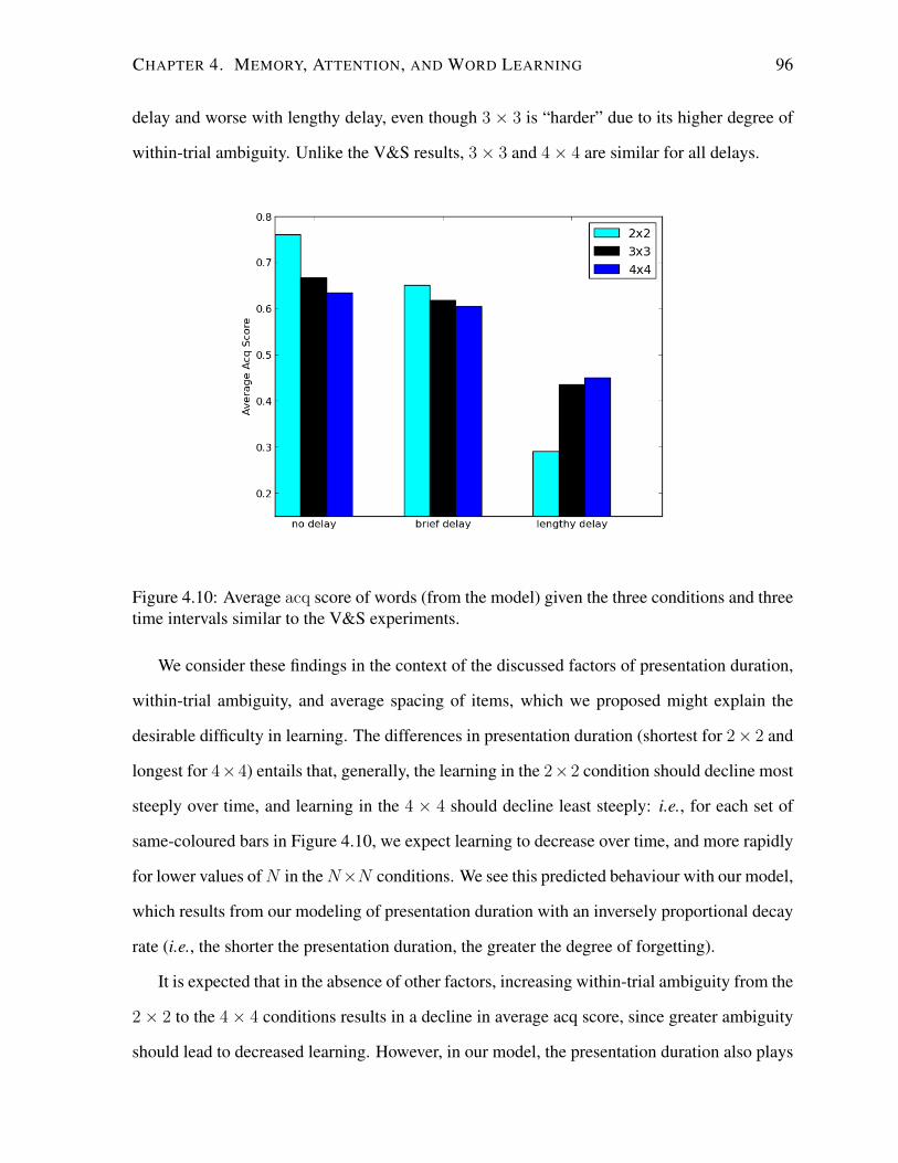
CHAPTER 4. MEMORY, ATTENTION, AND WORD LEARNING 96
delay and worse with lengthy delay, even though 3 × 3 is “harder” due to its higher degree of
within-trial ambiguity. Unlike the V&S results, 3× 3 and 4× 4 are similar for all delays.
Figure 4.10: Average acq score of words (from the model) given the three conditions and threetime intervals similar to the V&S experiments.
We consider these findings in the context of the discussed factors of presentation duration,
within-trial ambiguity, and average spacing of items, which we proposed might explain the
desirable difficulty in learning. The differences in presentation duration (shortest for 2× 2 and
longest for 4×4) entails that, generally, the learning in the 2×2 condition should decline most
steeply over time, and learning in the 4 × 4 should decline least steeply: i.e., for each set of
same-coloured bars in Figure 4.10, we expect learning to decrease over time, and more rapidly
for lower values ofN in theN×N conditions. We see this predicted behaviour with our model,
which results from our modeling of presentation duration with an inversely proportional decay
rate (i.e., the shorter the presentation duration, the greater the degree of forgetting).
It is expected that in the absence of other factors, increasing within-trial ambiguity from the
2× 2 to the 4× 4 conditions results in a decline in average acq score, since greater ambiguity
should lead to decreased learning. However, in our model, the presentation duration also plays
CHAPTER 4. MEMORY, ATTENTION, AND WORD LEARNING 97
a role. Similar to results of V&S, we see the decline pattern in the “no delay” condition, and
in the “brief delay” condition (albeit with less difference), due to the increased competition for
word–meaning alignments that occurs with a higher number of items in a trial (see Figure 4.10).
However, we do not see this pattern in the lengthy delay condition.
To summarize, our results are similar to those of V&S, who found that while the 2 × 2
condition led to best learning when tested immediately, it led to poorer performance than the
3×3 condition given a lengthy delay before testing — a pattern V&S attribute to the “desirable
difficulty”. It seems that these factors of presentation duration and within-trial ambiguity may
interact, such that the steep decline in performance in subsequent testing in the 2× 2 condition
more than offsets the advantage it has from the lesser within-trial ambiguity.
In the experiments of V&S, the performance in the 4 × 4 condition is always worse than
the two other conditions. However, our model produces very similar results for the 3 × 3 and
the 4 × 4 conditions. Also, the role of the spacing interval is not clear in these results. The
problem is that by just considering one set of stimuli within each N × N condition (each of
which has a specific set spacing of items), we do not have a variation of the average spacing
interval that is independent of the presentation duration and the within-trial ambiguity. We turn
to these issues in the next subsection.
4.5.3 Experiment 2: Randomly Generated Input
We observed that the performance of the model in the 3× 3 and 4× 4 conditions on the V&S
input is very similar. We also investigate a condition here with higher within-trial ambiguity
to see if such a condition might be “hard” enough for the model (because of the higher within-
trial ambiguity) so that it results in a similar pattern to the 4× 4 condition in V&S. As with the
others, we generate 20 sets of input stimuli for this 6×6 condition, using 18 word-object pairs,
each of which occurs 6 times, producing 18 trials. Thus the generated input stimuli for the four
conditions allows us to examine both the role of average spacing interval, and the impact of a
CHAPTER 4. MEMORY, ATTENTION, AND WORD LEARNING 98
more difficult condition with higher within-trial ambiguity.7
We train our model on the randomly-generated inputs (with different average spacing in-
tervals) for all four N ×N conditions. To evaluate the performance of the model, the average
acq score of words for all 20 sets of inputs within a single N ×N condition are averaged (see
Figure 4.11). We can see that when tested with “no delay”, the 2×2, 3×3, and 4×4 conditions
have similar scores. Moreover, we can see a pattern similar to V&S’s experiments: the 3 × 3
and 4 × 4 conditions have the best results after the “lengthy delay”. We also observe that by
increasing difficulty in the 6 × 6 condition (due to the high within-trial ambiguity), the model
produces a pattern similar to the pattern observed in the 4×4 condition in V&S’s experiments.
This confirms our hypothesis that for our model, the 4 × 4 condition is not “hard” enough to
result in a steep decline over time intervals as in the V&S’s results.
Figure 4.11: Average acq score of words (from the model) given the four conditions and thethree time intervals, averaged over 20 sets of stimuli.
However, we also see that, in contrast to V&S’s results (and our model’s performance on
the V&S data), the 2 × 2 condition with no delay fails to show better learning than the other7The forgetting decay parameter d (see Eqn. (4.7)) is set to 0.034 in the 6× 6 condition.
CHAPTER 4. MEMORY, ATTENTION, AND WORD LEARNING 99
conditions.
To better understand this difference between the two sets of results, we look more closely
at the scores of the individual randomly-generated stimuli sets. We find that there is a notable
difference in the average acq score across the 20 input files for the 2×2 condition, which shows
its maximum value of 0.76 for the V&S’s data, while the minimum is 0.50. This suggests that
the characteristics of the particular input (as a result of varying the average spacing interval)
may be responsible for some of the observed patterns in the V&S’s results.
We were interested to understand why the V&S 2 × 2 data has the maximum score, es-
pecially since there was a sizable gap between the score of this input and the next best score
among the randomly-generated inputs (of 0.64). In an attempt to identify the factor behind this
variation, we measured various statistics for each input set, such as the following: (1) the aver-
age spacing interval of words, which has been shown to affect learning both in people (Vlach
et al., 2008) and in our model (see Section 4.3); (2) average last occurrence time of words in
the input set, that impacts the amount of forgetting; and (3) the average context familiarity of
words (that is, the familiarity of the words that occur with a word in an utterance), a factor that
has been noted to affect word learning (see, e.g., Fazly et al. (2010a)).8 However, we found
that none of these measures explain the variation of the scores in all the inputs. Future research
is needed to fully understand the impact of the properties these measures tap into, and whether
they may (individually or in combination) contribute to explaining the pattern of the results.
4.5.4 Summary
The “desirable difficulty” of a learning condition can promote the long-term retention of the
learned items. We have used a computational model to investigate the possible factors be-
hind one such case of a “desirable difficulty” in a cross-situational word learning experiment
(Vlach and Sandhofer, 2010). Notably, the experimental results were not clearly pointing to
8We measure the familiarity of a word with its frequency of occurrence. The context familiarity of a word isthe average familiarity of words cooccurring with it in an utterance.
CHAPTER 4. MEMORY, ATTENTION, AND WORD LEARNING 100
the factors causing the patterns observed in the performance of the human participants. Using
a computational model, we have suggested that an interaction between two factors (the within-
trial ambiguity of the learning trials, and the presentation duration of each trial) might explain
the observed patterns. In addition, our results point to other distributional characteristics of
the input (experimental stimuli) that might have an impact on the performance of the learner.
These findings illustrate the role of computational modelling, not only in explaining observed
human behaviour, but also in fully understanding the factors involved in a phenomenon. There
are several factors involved in a cross-situational word learning experiment, such as the con-
textual familiarity of words, and the average spacing interval of words. Our findings signify
the importance of controlling for these factors in order to understand the reasons behind the ob-
served patterns. But it is difficult do so in human experiments because the factors can interact
in complex ways.
Our work is an initial attempt at shedding light on the interaction of memory, attention and
word learning, and understanding “desirable difficulty” in learning. Other factors (e.g., work-
ing memory) might play a role in the performance of people as well. For example, because the
number of items that people can store in their working memory is limited (Miller, 1956), the
participants might store more trials in their working memory in the 2× 2 condition, compared
with the other conditions. The participants might use this information of the multiple trials (in
their working memory) to make inferences about word–object mappings that repeat in succes-
sive trials. One future direction would be to incorporate a working memory module into our
word learning model, and examine the impact of such inferences in a cross-situational learning
scenario.
4.6 Conclusions
Much research has focused on understanding the spacing effect – the phenomenon that dis-
tributing (as opposed to cramming) learning events over a period of time significantly improves
CHAPTER 4. MEMORY, ATTENTION, AND WORD LEARNING 101
long-term learning. Yet the spacing effect is not precisely understood, i.e., how it arises from
cognitive processes (such as memory and attention). I have used our computational model to
identify potential cognitive causes and also to investigate their interactions, which is extremely
hard to achieve in experiments with human subjects. In our model, the interaction of forgetting
and attention to novelty explains the observed spacing effects in children and adults. I also
used our model to investigate the observation that – somewhat paradoxically – a more difficult
learning situation can result in better long-term learning. Our results suggest that the within-
trial ambiguity and the presentation duration of each trial in addition to other distributional
characteristics of the input (experimental stimuli) may explain these results. Our findings also
emphasize the role of computational modelling in understanding empirical results.
Chapter 5
Semantic Network Learning
Semantic development in children includes the acquisition of word-to-concept mappings (part
of word learning), and the formation of semantic connections among words/concepts. There
is considerable evidence that understanding the semantic properties of words improves child
vocabulary acquisition. In particular, children are sensitive to commonalities of semantic cat-
egories, and this abstract knowledge facilitates subsequent word learning (Jones et al., 1991;
Colunga and Smith, 2005). Furthermore, the representation of semantic knowledge is signif-
icant as it impacts how word meanings are stored in, searched for, and retrieved from mem-
ory (Steyvers and Tenenbaum, 2005; Griffiths et al., 2007).
As we discussed in Section 3.6, semantic knowledge is often represented as a graph (a se-
mantic network) in which nodes correspond to words/concepts, and edges specify the semantic
relations (Collins and Loftus, 1975; Steyvers and Tenenbaum, 2005). In our work here, we
assume that the nodes of a semantic network are words (with their learned meanings) and its
edges are determined by the semantic features of those words. Steyvers and Tenenbaum (2005)
demonstrated that a semantic network that encodes adult-level knowledge of words exhibits a
small-world and scale-free structure. That is, it is an overall sparse network with highly-
connected local sub-networks, where these sub-networks are connected through high-degree
hubs (nodes with many neighbours).
102
CHAPTER 5. SEMANTIC NETWORK LEARNING 103
Much experimental research has investigated the characteristics of semantic knowledge (Samuel-
son and Smith, 1999; Jones et al., 1991; Jones and Smith, 2005). However, existing compu-
tational models focus on certain aspects of semantic acquisition: Some researchers develop
computational models of word learning without considering the acquisition of semantic con-
nections that hold among words, or how this semantic knowledge is structured (Siskind, 1996;
Regier, 2005; Yu and Ballard, 2007; Frank et al., 2009; Fazly et al., 2010b). Another line
of work is to model formation of semantic categories but this work does not take into account
how word meanings/concepts are acquired (Anderson and Matessa, 1992; Griffiths et al., 2007;
Fountain and Lapata, 2011).
In this chapter, we extend our model to provide a cognitively-plausible and unified account
for both acquiring and representing semantic knowledge, in particular, simultaneously learning
words and creating a semantic network structure over them. The requirements for cognitive
plausibility enforce some constraints on the semantic network creation process. The first re-
quirement is incrementality, which means that the model gradually builds the network as it
processes the input. Also, the number of computations the model performs at each step must
be limited.
This chapter is organized as follows: Section 5.1 summarizes the relevant related work. In
Section 5.2, I present our algorithm for simultaneously learning word meanings and growing
a semantic network. Section 5.3 discusses how the resulting semantic networks are evaluated.
Finally, we examine networks created by our model under various conditions, and explore what
is required to obtain a structure that has appropriate semantic connections and has a small-
world and scale-free structure (Section 5.4 to Section 5.6). The work presented in this chapter
has been published in Nematzadeh et al. (2014b).
CHAPTER 5. SEMANTIC NETWORK LEARNING 104
5.1 Related Work
Models of Categorization. Several models have been proposed for learning categories over
words. Here, we focus on computational models that study categorization in humans. These
models form semantic clusters in an unsupervised manner given a defined set of features for
words (e.g., Anderson and Matessa, 1992; Griffiths et al., 2007; Sanborn et al., 2010). An-
derson and Matessa (1992) note that a cognitively plausible categorization algorithm needs
to be incremental and only keep track of one potential partitioning; they propose a Bayesian
framework (the Rational Model of Categorization or RMC) that specifies the joint distribution
on features and category labels, and allows an unbounded number of clusters. Sanborn et al.
(2010) examine different categorization models based on RMC. In particular, they compare
the performance of the approximation algorithm of Anderson and Matessa (1992) (local MAP)
with two other approximation algorithms (Gibbs Sampling and Particle Filters) in various hu-
man categorization paradigms. Sanborn et al. (2010) find that in most of the simulations the
local MAP algorithm performs as well as the two other algorithms in matching human behav-
ior.
The Structure of Semantic Knowledge. There is limited work on computational models
of semantic acquisition that examine the structure of the semantic knowledge. Steyvers and
Tenenbaum (2005) propose an algorithm for building a network with small-world and scale-
free structure. The algorithm starts with a small complete graph, incrementally adds new nodes
to the graph, and for each new node uses a probabilistic mechanism for selecting a subset of
current nodes to connect to. However, their approach does not address the problem of learning
word meanings or the semantic connections among them. Fountain and Lapata (2011) propose
an algorithm for learning categories that also creates a semantic network by comparing all the
possible word pairs; thus, it is not cognitively plausible. Moreover, they too do not address the
word learning problem, and do not investigate the structure of the learned semantic network to
see whether it has the properties observed in adult knowledge.
CHAPTER 5. SEMANTIC NETWORK LEARNING 105
5.2 The Incremental Network Model
We propose a model that unifies the incremental acquisition of word meanings and formation
of a semantic network structure over words (that reflects the semantic distances among their
learned meanings). Our model incrementally learns the meanings of words, and simultaneously
grows a semantic network using the developing word meanings.
5.2.1 Growing a Semantic Network
In our model, as we learn words incrementally (as explained in Section 2.4), we also structure
those words into a semantic network based on the (partially) learned meanings. At any given
point in time, the network will include as its nodes all the word types the word learner has
been exposed to. Weighted edges (capturing semantic distance) will connect those pairs of
word types whose learned meanings at that point are sufficiently semantically similar (i.e.,
their semantic distance is smaller than a threshold). Since the probabilistic meaning of a word
is adjusted each time it is observed, a word may either lose or gain connections in the network
after each input is processed. Thus, to incrementally develop the network, at each time step,
our algorithm must both examine existing connections (to see if any edges should be removed)
and consider potential new connections (to see if any edges should be added).
A simple approach to achieve this is to examine the current semantic distance between a
word w in the input and all the current words in the network, and include edges between only
those word pairs that are sufficiently similar. However, comparing allw ∈ U (current utterance)
to all words observed so far, every time an utterance is processed, is computationally intensive
(and not cognitively plausible).
We present an approach for incrementally growing a semantic network that limits the com-
putations when processing each input word w; see Algorithm 1. After the meaning of w is
updated, we first examine all the words that w is currently (directly) connected to: We check
if any of the edges between w and those words need to be removed (because their semantic
CHAPTER 5. SEMANTIC NETWORK LEARNING 106
distance falls above a threshold), or have their weight adjusted (because their distance changes
but is still below a threshold). Next, to look for new connections for w, the idea is to select
only a small subset (S) of observed words (V) to compare w with. Note that assuming S = V
provides “perfect” knowledge but also requires too much processing; thus, we choose S such
that |S| |V |. The challenge then is to select S in a way that will yield a network whose
semantic structure reasonably approximates the network that would result from full knowledge
of comparing w to all the words V .
Algorithm 1 Growing a network after each input u.for all w in u do
update P (·|w) using Eqn. (2.3)update current connections of wselect S(w), a subset of V , where V is all observed wordsfor all w′ in S(w) do
if dist(w,w′) < ζ thenconnect w and w′ with an edge of weight dist(w,w′)
end ifend for
end for
In determining a subset S of the observed vocabulary V to consider as potential words
for new connections to w, previous work has suggested picking “important” words for S in-
dependently of the target word w — e.g., words that are high-degree nodes in the network;
the assumption is that these may be words for which a learner might need to understand their
relationship to w in the future (Steyvers and Tenenbaum, 2005). Our proposal is instead to
consider for S those words that are likely to be similar to w. That is, since the network only
needs to connect w to similar words, if we can guess what (some of) those words are, then we
will do best at approximating the situation of comparing w to all words.
The question now is how to find semantically similar words to w that are not already con-
nected to w in the network. To do so, we incrementally track semantic similarity among words
usages as their meanings are developing. Specifically we cluster word tokens (not types) ac-
cording to their current word meanings. Since the probabilistic meanings of words are contin-
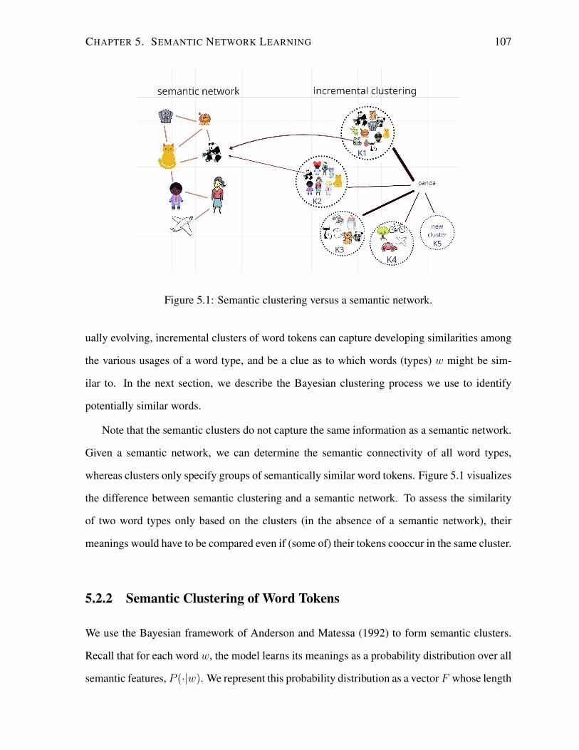
CHAPTER 5. SEMANTIC NETWORK LEARNING 107
Figure 5.1: Semantic clustering versus a semantic network.
ually evolving, incremental clusters of word tokens can capture developing similarities among
the various usages of a word type, and be a clue as to which words (types) w might be sim-
ilar to. In the next section, we describe the Bayesian clustering process we use to identify
potentially similar words.
Note that the semantic clusters do not capture the same information as a semantic network.
Given a semantic network, we can determine the semantic connectivity of all word types,
whereas clusters only specify groups of semantically similar word tokens. Figure 5.1 visualizes
the difference between semantic clustering and a semantic network. To assess the similarity
of two word types only based on the clusters (in the absence of a semantic network), their
meanings would have to be compared even if (some of) their tokens cooccur in the same cluster.
5.2.2 Semantic Clustering of Word Tokens
We use the Bayesian framework of Anderson and Matessa (1992) to form semantic clusters.
Recall that for each word w, the model learns its meanings as a probability distribution over all
semantic features, P (·|w). We represent this probability distribution as a vector F whose length
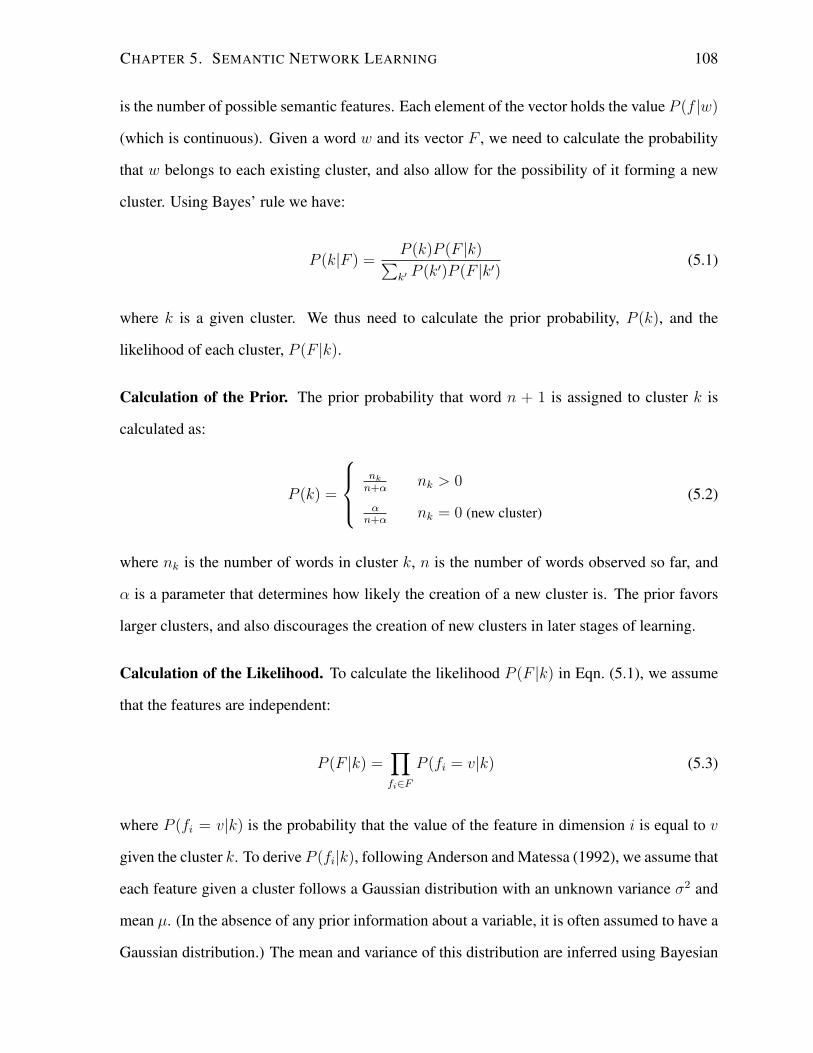
CHAPTER 5. SEMANTIC NETWORK LEARNING 108
is the number of possible semantic features. Each element of the vector holds the value P (f |w)
(which is continuous). Given a word w and its vector F , we need to calculate the probability
that w belongs to each existing cluster, and also allow for the possibility of it forming a new
cluster. Using Bayes’ rule we have:
P (k|F ) =P (k)P (F |k)∑k′ P (k′)P (F |k′)
(5.1)
where k is a given cluster. We thus need to calculate the prior probability, P (k), and the
likelihood of each cluster, P (F |k).
Calculation of the Prior. The prior probability that word n + 1 is assigned to cluster k is
calculated as:
P (k) =
nk
n+αnk > 0
αn+α
nk = 0 (new cluster)(5.2)
where nk is the number of words in cluster k, n is the number of words observed so far, and
α is a parameter that determines how likely the creation of a new cluster is. The prior favors
larger clusters, and also discourages the creation of new clusters in later stages of learning.
Calculation of the Likelihood. To calculate the likelihood P (F |k) in Eqn. (5.1), we assume
that the features are independent:
P (F |k) =∏fi∈F
P (fi = v|k) (5.3)
where P (fi = v|k) is the probability that the value of the feature in dimension i is equal to v
given the cluster k. To derive P (fi|k), following Anderson and Matessa (1992), we assume that
each feature given a cluster follows a Gaussian distribution with an unknown variance σ2 and
mean µ. (In the absence of any prior information about a variable, it is often assumed to have a
Gaussian distribution.) The mean and variance of this distribution are inferred using Bayesian
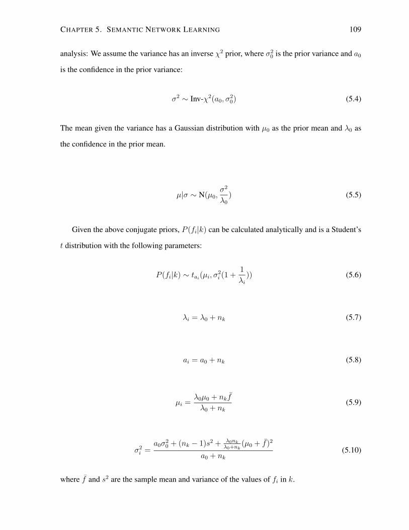
CHAPTER 5. SEMANTIC NETWORK LEARNING 109
analysis: We assume the variance has an inverse χ2 prior, where σ20 is the prior variance and a0
is the confidence in the prior variance:
σ2 ∼ Inv-χ2(a0, σ20) (5.4)
The mean given the variance has a Gaussian distribution with µ0 as the prior mean and λ0 as
the confidence in the prior mean.
µ|σ ∼ N(µ0,σ2
λ0) (5.5)
Given the above conjugate priors, P (fi|k) can be calculated analytically and is a Student’s
t distribution with the following parameters:
P (fi|k) ∼ tai(µi, σ2i (1 +
1
λi)) (5.6)
λi = λ0 + nk (5.7)
ai = a0 + nk (5.8)
µi =λ0µ0 + nkf
λ0 + nk(5.9)
σ2i =
a0σ20 + (nk − 1)s2 + λ0nk
λ0+nk(µ0 + f)2
a0 + nk(5.10)
where f and s2 are the sample mean and variance of the values of fi in k.
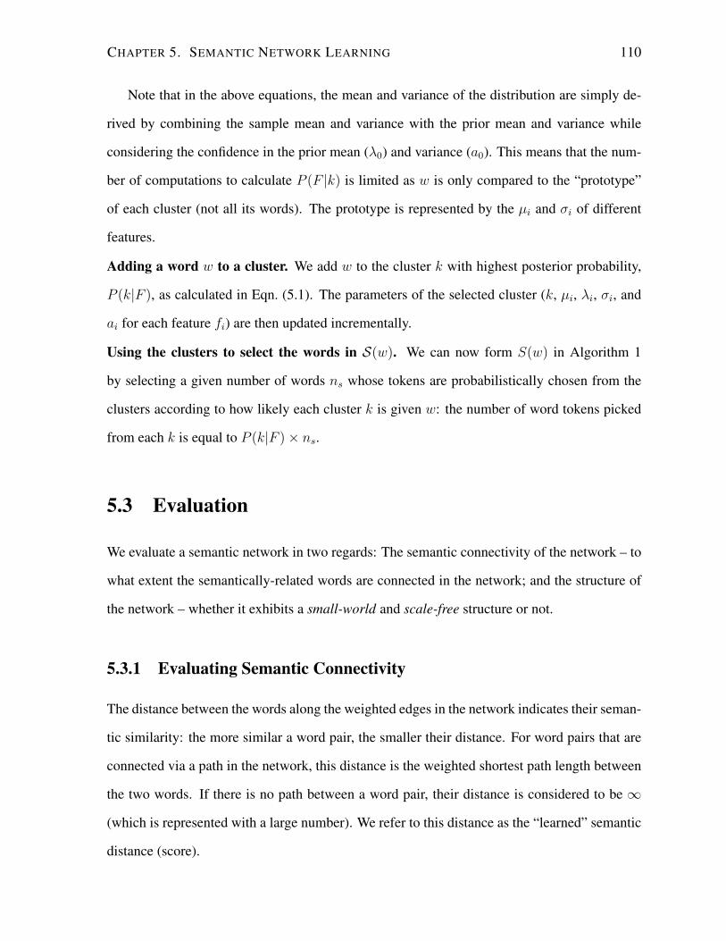
CHAPTER 5. SEMANTIC NETWORK LEARNING 110
Note that in the above equations, the mean and variance of the distribution are simply de-
rived by combining the sample mean and variance with the prior mean and variance while
considering the confidence in the prior mean (λ0) and variance (a0). This means that the num-
ber of computations to calculate P (F |k) is limited as w is only compared to the “prototype”
of each cluster (not all its words). The prototype is represented by the µi and σi of different
features.
Adding a word w to a cluster. We add w to the cluster k with highest posterior probability,
P (k|F ), as calculated in Eqn. (5.1). The parameters of the selected cluster (k, µi, λi, σi, and
ai for each feature fi) are then updated incrementally.
Using the clusters to select the words in S(w). We can now form S(w) in Algorithm 1
by selecting a given number of words ns whose tokens are probabilistically chosen from the
clusters according to how likely each cluster k is given w: the number of word tokens picked
from each k is equal to P (k|F )× ns.
5.3 Evaluation
We evaluate a semantic network in two regards: The semantic connectivity of the network – to
what extent the semantically-related words are connected in the network; and the structure of
the network – whether it exhibits a small-world and scale-free structure or not.
5.3.1 Evaluating Semantic Connectivity
The distance between the words along the weighted edges in the network indicates their seman-
tic similarity: the more similar a word pair, the smaller their distance. For word pairs that are
connected via a path in the network, this distance is the weighted shortest path length between
the two words. If there is no path between a word pair, their distance is considered to be ∞
(which is represented with a large number). We refer to this distance as the “learned” semantic
distance (score).
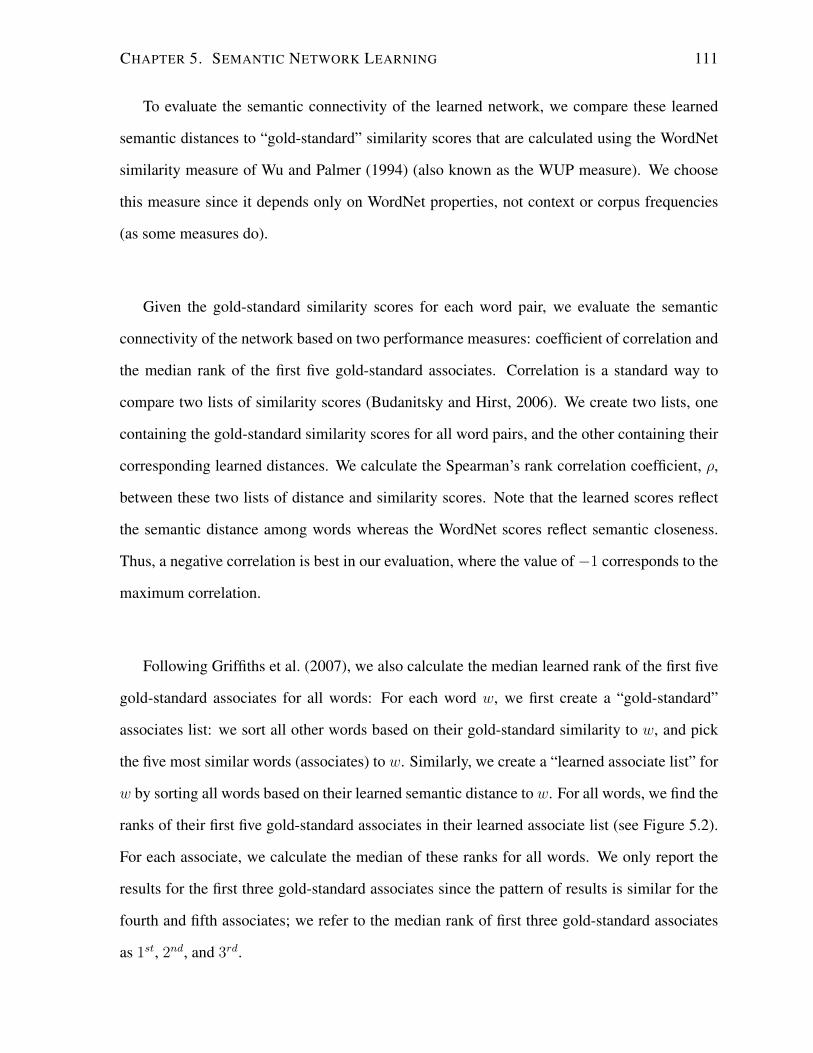
CHAPTER 5. SEMANTIC NETWORK LEARNING 111
To evaluate the semantic connectivity of the learned network, we compare these learned
semantic distances to “gold-standard” similarity scores that are calculated using the WordNet
similarity measure of Wu and Palmer (1994) (also known as the WUP measure). We choose
this measure since it depends only on WordNet properties, not context or corpus frequencies
(as some measures do).
Given the gold-standard similarity scores for each word pair, we evaluate the semantic
connectivity of the network based on two performance measures: coefficient of correlation and
the median rank of the first five gold-standard associates. Correlation is a standard way to
compare two lists of similarity scores (Budanitsky and Hirst, 2006). We create two lists, one
containing the gold-standard similarity scores for all word pairs, and the other containing their
corresponding learned distances. We calculate the Spearman’s rank correlation coefficient, ρ,
between these two lists of distance and similarity scores. Note that the learned scores reflect
the semantic distance among words whereas the WordNet scores reflect semantic closeness.
Thus, a negative correlation is best in our evaluation, where the value of −1 corresponds to the
maximum correlation.
Following Griffiths et al. (2007), we also calculate the median learned rank of the first five
gold-standard associates for all words: For each word w, we first create a “gold-standard”
associates list: we sort all other words based on their gold-standard similarity to w, and pick
the five most similar words (associates) to w. Similarly, we create a “learned associate list” for
w by sorting all words based on their learned semantic distance to w. For all words, we find the
ranks of their first five gold-standard associates in their learned associate list (see Figure 5.2).
For each associate, we calculate the median of these ranks for all words. We only report the
results for the first three gold-standard associates since the pattern of results is similar for the
fourth and fifth associates; we refer to the median rank of first three gold-standard associates
as 1st, 2nd, and 3rd.
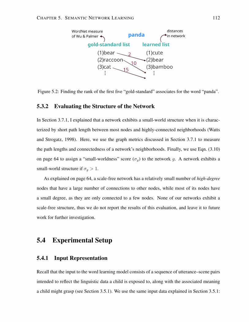
CHAPTER 5. SEMANTIC NETWORK LEARNING 112
Figure 5.2: Finding the rank of the first five “gold-standard” associates for the word “panda”.
5.3.2 Evaluating the Structure of the Network
In Section 3.7.1, I explained that a network exhibits a small-world structure when it is charac-
terized by short path length between most nodes and highly-connected neighborhoods (Watts
and Strogatz, 1998). Here, we use the graph metrics discussed in Section 3.7.1 to measure
the path lengths and connectedness of a network’s neighborhoods. Finally, we use Eqn. (3.10)
on page 64 to assign a “small-worldness” score (σg) to the network g. A network exhibits a
small-world structure if σg > 1.
As explained on page 64, a scale-free network has a relatively small number of high-degree
nodes that have a large number of connections to other nodes, while most of its nodes have
a small degree, as they are only connected to a few nodes. None of our networks exhibit a
scale-free structure, thus we do not report the results of this evaluation, and leave it to future
work for further investigation.
5.4 Experimental Setup
5.4.1 Input Representation
Recall that the input to the word learning model consists of a sequence of utterance–scene pairs
intended to reflect the linguistic data a child is exposed to, along with the associated meaning
a child might grasp (see Section 3.5.1). We use the same input data explained in Section 3.5.1:
CHAPTER 5. SEMANTIC NETWORK LEARNING 113
We use the Manchester corpus (Theakston et al., 2001), which consists of transcripts of conver-
sations with 12 British children between the ages of 1; 8 and 3; 0. We represent each utterance
as a bag of lemmatized words. We automatically generate the scene associated with an ut-
terance U, using a scheme introduced in Section 3.5.1: We use an input-generation lexicon
containing the “gold-standard” meaning gs(w) (a vector of semantic features and their scores)
for each word w in our corpus (see Figure 3.6). We probabilistically sample an observed subset
of features from the full set of features in gs(w) for each word w ∈ U. The scene S is the union
of all the features sampled for all the words in the utterance.
5.4.2 Methods
We experiment with our network-growth method that draws on the incremental clustering,
and create “upper-bound” and baseline networks for comparison. Note that all the networks
are created using our Algorithm 1 (page 106) to grow networks incrementally, drawing on
the learned meanings of words and updating their connections on the basis of this evolving
knowledge. The only difference in creating the networks resides in how the comparison set
S(w) is chosen for each target word w that is being processed at each time step. We provide
more details in the paragraphs below.
Upper-bound. Recall that one of our main goals is to substantially reduce the number of
similarity comparisons needed to grow a semantic network, in contrast to the straightforward
method of comparing each w in the current utterance to all previously observed words. At the
same time, we need to understand the impact of the increased efficiency on the quality of the
resulting networks. We thus need to compare the target properties of our networks that are
learned using a small comparison set S, to those of an “upper-bound” network that takes into
account all the pair-wise comparisons among words. We create this upper-bound network by
setting S(w) to contain all words currently in the network (i.e., all words previously observed
by the model).
CHAPTER 5. SEMANTIC NETWORK LEARNING 114
Baselines. On the other hand, we need to evaluate the (potential) benefit of our cluster-driven
selection process over a more simplistic approach to selecting S(w). To do so, we consider
three baselines, each using a different criterion for choosing the comparison set S(w): The
Random baseline chooses the members of this set randomly from the set of all observed words.
The Context baseline can be seen as an “informed” baseline that attempts to incorporate some
semantic knowledge: Here, we select words that are in the recent context prior to w in the
input, assuming that such words are likely to be semantically related to w. We also include
a third baseline, Random+Context, that picks half of the members of S randomly and half of
them from the prior context.
Cluster-based Methods. We report results for three cluster-based networks that differ in
their choice of S(w) as follows: The Clusters-only network chooses words for S(w) from the
set of clusters, proportional to the probability of each cluster k given word w (as explained in
Section 5.2.2). In order to incorporate different types of semantic information in selecting S,
we also create a Clusters+Context network that picks half of the members of S from clusters
(as above), and half from the prior context. For completeness, we include a Clusters+Random
network that similarly chooses half of the words in S from clusters and half randomly from all
observed words.
We have experimented with several other methods, but they all performed substantially
worse than the baselines, and hence we do not report them here. For example, we tried picking
words in S from the best single cluster (i.e., argmaxkP (k|F )). We also tried a few methods
inspired by Steyvers and Tenenbaum (2005): E.g., we examined a method where if a member
of S(w) was sufficiently similar to w, we added the direct neighbors of that word to S as
well. We also tried to grow networks by choosing the members of S according to the degree
or frequency of nodes in the network. None of these methods for composing S(w) performed
reasonably.
CHAPTER 5. SEMANTIC NETWORK LEARNING 115
5.4.3 Experimental Parameters
We use 20, 000 utterance–scene pairs as our training data. We use only nouns in growing the
semantic networks (as in Section 3.7.2). This is because the semantic features of different parts
of speech (POS) are drawn from different sources, thus the similarity of two words with differ-
ent POS’s cannot be reliably measured. There are 1074 nouns in each final network. Recall that
we use clustering to help guide our semantic network growth algorithm. Given the clustering
algorithm in Section 5.2.2, we are interested to find the best set of clusters for our data. To
do we perform a search on the parameter space, and select the parameter values that result in
the best clustering, based on the number of clusters and their average F-score. (Note that any
incremental clustering algorithm can be used here.) The value of the clustering parameters are
as follows: α = 49, λ0 = 1.0, a0 = 2.0, µ0 = 0.0, and σ0 = 0.05. Two nouns with feature
vectors F1 and F2 are connected in the network if cosine(F1, F2) is greater than or equal to
0.6. (This threshold was selected following empirical examination of the similarity values we
observe among the “gold-standard” meanings in our gold-standard lexicon.) The weight on
the edge that connects these nouns specifies their semantic distance, which is calculated as
1− cosine(F1, F2).
Recall that we aim for network creation methods that have a limited number of word-to-
word comparisons. To have comparable methods for selecting the subset S, we need to ensure
that all the different methods yield roughly similar numbers of such comparisons. Keeping the
size of S constant does not guarantee this, because at each point in time, the number of existing
connections of the target word w, (and consequently the number of comparisons required to
update these connections) vary across different methods. We thus parameterize the size of S
for each method to keep the number of computations similar, based on experiments on the
development data. In development work we also found that having an increasing size of S
over time improved the results, as more words were compared as the knowledge of learned
meanings improved. To achieve this, we use a percentage of the words in the network as the
size of S. In practice, the setting of this parameter yields a number of comparisons across all
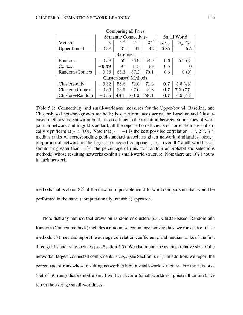
CHAPTER 5. SEMANTIC NETWORK LEARNING 116
Comparing all PairsSemantic Connectivity Small World
Method ρ 1st 2nd 3rd sizelcc σg (%)Upper-bound −0.38 31 41 42 0.85 5.5
BaselinesRandom −0.38 56 76.9 68.9 0.6 5.2 (2)Context −0.39 97 115 89 0.5 0Random+Context −0.36 63.3 87.2 79.1 0.6 0 (0)
Cluster-based MethodsClusters-only −0.32 58.6 72.0 71.6 0.7 5.5 (43)Clusters+Context −0.36 53.9 67.6 64.8 0.7 7.2 (77)Clusters+Random −0.35 48.1 61.2 58.1 0.7 6.9 (48)
Table 5.1: Connectivity and small-worldness measures for the Upper-bound, Baseline, andCluster-based network-growth methods; best performances across the Baseline and Cluster-based methods are shown in bold. ρ: co-efficient of correlation between similarities of wordpairs in network and in gold-standard; all the reported co-efficients of correlation are statisti-cally significant at p < 0.01. Note that ρ = −1 is the best possible correlation. 1st, 2nd, 3rd:median ranks of corresponding gold-standard associates given network similarities; sizelcc:proportion of network in the largest connected component; σg: overall “small-worldness”,should be greater than 1; %: the percentage of runs (for random or probabilistic selectionsmethods) whose resulting networks exhibit a small-world structure. Note there are 1074 nounsin each network.
methods that is about 8% of the maximum possible word-to-word comparisons that would be
performed in the naive (computationally intensive) approach.
Note that any method that draws on random or clusters (i.e., Cluster-based, Random and
Random+Context methods) includes a random selection mechanism; thus, we run each of these
methods 50 times and report the average correlation coefficient ρ and median ranks of the first
three gold-standard associates (see Section 5.3). We also report the average relative size of the
networks’ largest connected components, sizelcc (see Section 3.7.1). In addition, we report the
percentage of runs whose resulting network exhibit a small-world structure. For the networks
(out of 50 runs) that exhibit a small-world structure (small-worldness greater than one), we
report the average small-worldness.
CHAPTER 5. SEMANTIC NETWORK LEARNING 117
5.5 Experimental Results
Table 5.1 presents our results, including the evaluation measures explained above, for the
Upper-bound, Baseline, and Cluster-based networks created by the various methods described
in Section 5.4.2.
Recall that the Upper-bound network is formed from comparing a word’s similarity to
all other (observed) words when the word is being processed. We can see that this network is
highly connected (0.85) and has a small-world structure (5.5). There is a statistically significant
correlation of the network’s similarity measures with the gold standard ones (−0.38). For this
Upper-bound structure, the median ranks of the first three associates are between 31 and 42.
These latter two measures on the Upper-bound network give an indication of the difficulty of
learning a semantic network whose knowledge matches gold-standard similarities.
Considering the baseline networks, we note that the Random network is actually somewhat
better (in connectivity and median ranks) than the Context network that we thought would
provide a more informed baseline. Interestingly, the correlation value for both networks is no
worse than for the Upper-bound. The combination of Random+Context yields a slightly lower
correlation, and no better ranks or connectivity than Random. Note that none of the baseline
networks exhibit a small world structure (σg 1 for all three, except for one out of 50 runs
for the Random method).
Recall that the Random network is not a network resulting from randomly connecting word
pairs, but one that incrementally compares each target word with a set of randomly chosen
words when considering possible new connections. We suspect that this approach performs
reasonably well because it enables the model to find a broad range of similar words to the
target; this might be effective especially because the learned meanings of words are changing
over time.
Turning to the Cluster-based methods, we see that indeed some diversity in the comparison
set for a target word might be necessary to good performance. We find that the measures on
the Clusters-only network are roughly the same as on the Random one, but when we combine
CHAPTER 5. SEMANTIC NETWORK LEARNING 118
the two in Clusters+Random we see an improvement in the ranks achieved. It is possible that
the selection from clusters does not have sufficient diversity to find some of the valid new
connections for a word.
We note that the best results overall occur with the Clusters+Context network, which com-
bines two approaches to selecting words that have good potential to be similar to the target
word. The correlation coefficient for this network is at a respectable 0.36, and the median
ranks are the second best of all the network-growth methods. Importantly, this network shows
the desired small-world structure in most of the runs (77%), with the highest connectivity and
a small-world measure well over 1.
The fact that the Clusters+Context network is better overall than the networks of the Clusters-
only and Context methods indicates that both clusters and context are important in making “in-
formed guesses” about which words are likely to be similar to a target word. Given the small
number of similarity comparisons used in our experiments (only around 8% of all possible
word-to-word comparisons), these observations suggest that both the linguistic context and the
evolving relations among word usages (captured by the incremental clustering of learned mean-
ings) contain information crucial to the process of growing a semantic network in a cognitively
plausible way.
5.6 Conclusions
We propose a unified model of word learning and semantic network formation, which creates
a network of words in which connections reflect structured knowledge of semantic distance
between words. The model adheres to the cognitive plausibility requirements of incrementality
and use of limited computations. That is, when incrementally adding or updating a word’s
connections in the network, the model only looks at a subset of words rather than comparing
the target word to all the nodes in the network. For a given word, this subset of words is
selected by taking advantage of the semantic relations among words in addition to the context
CHAPTER 5. SEMANTIC NETWORK LEARNING 119
of the word. To capture the semantic relations among words, the model incrementally forms
semantic clusters as it processes each word. We demonstrate that using the evolving knowledge
of semantic connections among words (which is captured in the developing semantic clusters)
as well as their context of usage enables the model to create a network that shows the properties
of adult semantic knowledge.
Chapter 6
Conclusions
Child word learning is a complex process that we do not fully understand. This thesis in-
vestigates the role of cognitive processes in vocabulary development through computational
modeling. I have designed and developed a computational model that mimics child vocabulary
development; it incrementally learns the meaning of words along with the semantic connec-
tions among them. In building this model, I have assumed that the domain-general learning
mechanisms are sufficient for word learning: the model employs general statistical learning
mechanisms. Moreover, in the model, word learning is naturally integrated with other cog-
nitive processes such as memory and attention. This thesis demonstrates the importance of
modeling word learning in the context of cognitive processes by examining three different phe-
nomena that I review in the next section. I then discuss a number of interesting directions for
future research.
6.1 Summary of Contributions
Individual differences in word learning (Nematzadeh et al., 2011, 2012b, 2014a). Late talk-
ers are children who show a marked delay in vocabulary learning. Since these children are at
risk for specific language impairment, identifying factors involved in late talking is a significant
research problem. Previous research has identified different cognitive factors that might con-
120
CHAPTER 6. CONCLUSIONS 121
tribute to late talking. To examine the underlying factors behind late talking, we propose a com-
putational word learner that simulates a child’s attentional development. By varying the rate
of attentional development, our model simulates a continuum of learners mimicking normally-
developing, temporarily delayed, and language-impaired children. Our simulated late-talking
learners, similar to late-talking children, exhibit a delayed and slower vocabulary growth in ad-
dition to a less semantically-connected vocabulary compared to normally-developing children.
We extend our model with a categorization mechanism to further study how individual dif-
ferences between learners give rise to differences in abstract knowledge of categories emerging
from learned words, and how this affects their subsequent word learning. Our results suggest
that the vocabulary composition of late-talking and normally-developing learners differ at least
partially due to a deficit in the attentional abilities of late-talking learners, which also results in
the learning of weaker abstract knowledge of semantic categories of words.
Moreover, we use our model to examine the structure of each learner’s semantic network
(which represents words and the relations among them). The structure of this network is signif-
icant as it might reveal aspects of the developmental process that leads to the network. We find
that the learned semantic knowledge of a learner that simulates a normally-developing child
reflects the structural properties found in adult semantic networks of words. In contrast, the
network of a late-talking learner does not exhibit these properties.
The role of forgetting in word learning (Nematzadeh et al., 2012a, 2013b). There is con-
siderable evidence that people generally learn items better when the presentation of items is
distributed over a period of time (the spacing effect). We hypothesize that both forgetting and
attention to novelty play a role in the spacing effect in word learning. We extend our word
learning model with forgetting and attentional mechanisms. We show that the interaction of
these mechanisms in our model explains several patterns of spacing effect observed in children
and adults.
Moreover, we use our model to examine the possible explanatory factors behind desirable
difficulties in a cross-situational word learning experiment where difficulties of the word learn-
CHAPTER 6. CONCLUSIONS 122
ing situation promote long-term learning. Our results suggest that the within-trial ambiguity
and the presentation duration of each trial in addition to other distributional characteristics of
the input (experimental stimuli) may explain these results.
Learning semantic networks (Nematzadeh et al., 2014b). Semantic knowledge is often pre-
sented as a network in which the nodes are words and the edges specify their semantic relations.
An important open question is how such a semantic network can be gradually acquired as word
meanings are learned. I have designed and implemented an algorithm that incrementally and
efficiently grows a semantic network by tapping into the evolving probabilistic relations among
the words. Our model is successful in creating networks that reflect the quality and structure
of adult semantic knowledge. Its success stems from incorporation of the evolving knowledge
of semantic categories and information inherent in the context of words.
6.2 Future Directions
This section presents some possible future directions for this line of research. These directions
are organized by increased complexity, discussing short-term extensions first, and long-term
goals next.
6.2.1 Short-term Extensions
Novel word generalization. A key challenge faced by children in vocabulary acquisition is
learning which of the many possible meanings is appropriate for a word. The word general-
ization problem refers to how children associate a word such as dog with a meaning at the
appropriate category level in the taxonomy of objects, such as Dalmatians, dogs, or animals. A
possible future direction is to extend our word learning model to account for the word general-
ization problem. In an ongoing project, we address this problem by providing a unified account
CHAPTER 6. CONCLUSIONS 123
of word generalization and word learning within our computational model of cross-situational
learning. Our model – without incorporating any additional biases and simply through learning
meanings for words – replicates the patterns observed in child and adult word generalization.
The model simulates child patterns of word generalization due to the interaction of type and
token frequencies in the input data, an influence often observed in usage-based approaches to
underlie people’s generalization of linguistic categories.
Modeling social and pragmatic attentional cues. The environment of a child is enriched with
different sources of information that can facilitate language learning; in addition to the linguis-
tic and visual input, a child perceives social and pragmatic attentional cues such as eye gaze,
pointing, and the prosody of speech. Our previous work (Beekhuizen et al., 2013) shows that
these attentional cues might be particularly significant in the acquisition of words for which
there is not enough cross-situational evidence available (such as relational words). An in-
teresting future direction is to investigate the role of these attentional cues in acquisition of
different groups of words. My dissertation takes a step towards this direction. I have extended
our word learning model to include an attentional mechanism that simulates a limited number
of attentional factors. This attentional mechanism is embedded in the model’s calculation of
word-meaning probabilities. Maintaining the overall probabilistic formulation of the model is
the key challenge in generalizing this attentional mechanism to other attentional cues.
6.2.2 Long-term Goals
Discovering relations among words. Over the course of language learning, children discover
various relation types among words, such as semantic similarity (e.g., “cat” and “dog”), re-
latedness (e.g., “cat” and “milk”), and meronomy (“wheel” and “car”). These relations help
children in learning novel words, and also in comprehending the meaning of larger linguistic
units such as phrases and sentences. A common theme in my previous research for learning
CHAPTER 6. CONCLUSIONS 124
such relations is identifying the usage patterns and statistical regularities that indicate the rela-
tions. For example, our semantic network formation model captures one type of these relations
(i.e., semantic similarity) by drawing on regularities in evolving word meanings. Moreover,
our model acquires multiword verbs by tapping into the statistical regularities of certain lin-
guistic structures (Nematzadeh et al., 2013a). I plan to extend this approach to investigate how
children acquire other types of relations. These relations could often be identified by tracking
some cooccurrence patterns unique to the relation. Devising such patterns is tedious and track-
ing them individually alongside word-meaning mappings is not scalable. One possibility is to
investigate using the word meanings – that are highly contextualized – to extract this necessary
information.
Learning meaning representations for sentences. Understanding the meaning of individual
words and their semantic relations (such as those explained above) is not sufficient for com-
prehending the meaning of sentences. To understand a sentence’s meaning, children need to
recognize how the meaning of its words relate and interact. Consider the sentences “Sebastian
ate the apple” and “The apple was eaten by Sebastian”. To recognize that these sentences ex-
press similar information, a computational model needs to (1) know the word meanings, and
(2) identify the thematic relations between verbs and their arguments, i.e., how noun phrases
relate to the verbs: in both sentences, despite the difference in word orders, “Sebastian” per-
formed the action of eating, and “apple” was the recipient of the action. To recognize these
thematic relations, a model needs to learn the commonalities across the subjects of a verb, e.g.,
“eaters” are often animate. Moreover, it needs to learn the regularities over different verbs,
e.g., certain verbs require an animate subject. I plan to learn these two different levels of ab-
straction by forming hierarchical clusters that group similar usages of verbs. The novelty of
this approach is in using word meanings in addition to several other semantic and syntactic
features, such as the position of a noun with respect to the verb, and any preposition used with
the verb. Simultaneous learning of word meanings and these thematic relations enables the
CHAPTER 6. CONCLUSIONS 125
model to provide rich meaning representations for sentences.
6.3 Concluding Remarks
Computational modeling is a powerful tool for studying language acquisition, and has gained
tremendous popularity in the last decade. Throughout this thesis, I have used computational
modeling to investigate how vocabulary development interacts with other cognitive processes.
I believe that instead of building small independent models that only explain some specific
data, we need to design unified models that account for all the “significant” data available
for a given phenomenon. Such frameworks, when evaluated throughly, can produce reliable
predictions. The work of this thesis is in line with this research philosophy: Our computational
model replicates several patterns observed in word learning, and produces novel predictions.
Because it is used to examine various aspects of word learning, our model provides a general
framework for studying vocabulary development.

Bibliography
J. T. Abbott, J. L. Austerweil, and T. L. Griffiths. Constructing a hypothesis space from the
web for large-scale Bayesian word learning. Proceedings of the 34th Annual Conference of
the Cognitive Science Society, 2012.
A. Alishahi and A. Fazly. Integrating syntactic knowledge into a model of cross-situational
word learning. In Proceedings of the 32nd Annual Conference of the Cognitive Science
Society, 2010.
A. Alishahi, A. Fazly, and S. Stevenson. Fast mapping in word learning: What probabilities tell
us. In Proceedings of the Twelfth Conference on Computational Natural Language Learning,
pages 57–64. Association for Computational Linguistics, 2008.
J. R. Anderson and C. Lebiere. The atomic components of thought. Lawrence Erlbaum Asso-
ciates, 1998.
J. R. Anderson and M. Matessa. Explorations of an incremental Bayesian algorithm for cate-
gorization. Machine Learning, 9(4):275–308, 1992.
H. P. Bahrick. Maintenance of knowledge: Questions about memory we forgot to ask. Journal
of Experimental Psychology: General, 108(3):296–308, 1979.
H. P. Bahrick and E. Phelps. Retention of Spanish vocabulary over 8 years. Journal of Experi-
mental Psychology: Learning, Memory, and Cognition, 13(2):344–349, 1987.
126
BIBLIOGRAPHY 127
N. Beckage, L. B. Smith, and T. Hills. Semantic network connectivity is related to vocabulary
growth in children. In Proceedings of the 32nd Annual Conference of the Cognitive Science
Society, 2010.
N. Beckage, L. B. Smith, and T. Hills. Small worlds and semantic network growth in typical
and late talkers. PloS one, 6(5):e19348, 2011.
B. Beekhuizen, A. Fazly, A. Nematzadeh, and S. Stevenson. Word learning in the wild: What
natural data can tell us. In Proceedings of the 35th Annual Conference of the Cognitive
Science Society, pages 1857–1862, 2013.
H. Benedict. Early lexical development: Comprehension and production. Journal of Child
Language, 6(2):183–200, 1979.
R. A. Bjork. Memory and metamemory considerations in the training of human beings. In J. E.
Metcalfe and A. P. Shimamura, editors, Metacognition: Knowing about knowing., pages
185–205. The MIT Press, 1994.
L. Bloom. One word at a time: The use of single word utterances before syntax, volume 154.
Mouton The Hague, 1973.
P. F. Brown, S. A. Della Pietra, V. J. Della Pietra, and R. L. Mercer. The mathematics of
statistical machine translation: Parameter estimation. Computational Linguistics, 19(2):
263–311, 1993.
A. Budanitsky and G. Hirst. Evaluating wordnet-based measures of lexical semantic related-
ness. Computational Linguistics, 32(1):13–47, 2006.
S. Carey. The child as word learner. In M. Halle, J. Bresnan, and G. A. Miller, editors,
Linguistic Theory and Psychological Reality. The MIT Press, 1978.
S. Carey and E. Bartlett. Acquiring a single new word. In Proceedings of the Stanford Child
Language Conference, volume 15, pages 17–29, 1978.
BIBLIOGRAPHY 128
N. J. Cepeda, H. Pashler, E. Vul, J. T. Wixted, and D. Rohrer. Distributed practice in verbal
recall tasks: A review and quantitative synthesis. Psychological Bulletin, 132(3):354 – 380,
2006.
N. Chomsky. On the nature, use, and acquisition of language. MIT Press, 1993.
A. M. Collins and E. F. Loftus. A spreading-activation theory of semantic processing. Psycho-
logical Review, 82(6):407, 1975.
E. Colunga and C. Sims. Early talkers and late talkers know nouns that license different word
learning biases. In Proceedings of the 33th Annual Conference of the Cognitive Science
Society, 2011.
E. Colunga and L. B. Smith. From the lexicon to expectations about kinds: A role for associa-
tive learning. Psychological Review, 112(2):347–382, 2005.
L. J. Cuddy and L. L. Jacoby. When forgetting helps memory: an analysis of repetition effects.
Journal of Verbal Learning and Verbal Behavior, 21(4):451 – 467, 1982.
F. Dempster. Spacing effects and their implications for theory and practice. Educational
Psychology Review, 1:309–330, 1989.
F. N. Dempster. Distributing and managing the conditions of encoding and practice. Memory,
pages 317–344, 1996.
J. Deng, W. Dong, R. Socher, L.-J. Li, K. Li, and L. Fei-Fei. Imagenet: A large-scale hier-
archical image database. In IEEE Conference on Computer Vision and Pattern Recognition
(CVPR), pages 248–255. IEEE, 2009.
C. Desmarais, A. Sylvestre, F. Meyer, I. Bairati, and N. Rouleau. Systematic review of the
literature on characteristics of late-talking toddlers. International Journal of Language and
Communication Disorders, 43(4):361–389, 2008.
BIBLIOGRAPHY 129
H. Ebbinghaus. Memory: A contribution to experimental psychology. New York, Teachers
College, Columbia University, 1885.
J. Elman. Computational approaches to language acquisition. Encyclopedia of Language and
Linguistics,, 2:726–732, 2006.
P. Erdos and A. Renyi. On the evolution of random graphs. Publications of the Mathematical
Institute of the Hungarian Academy of Sciences, 5:17–61, 1960.
J. Evans, J. Saffran, and K. Robe-Torres. Statistical learning in children with specific language
impairment. Journal of Speech, Language and Hearing Research, 52(2):321, 2009.
A. Fazly and S. Stevenson. Distinguishing subtypes of multiword expressions using
linguistically-motivated statistical measures. In Proceedings of the Workshop on A Broader
Perspective on Multiword Expressions, pages 9–16. Association for Computational Linguis-
tics, 2007.
A. Fazly, A. Alishahi, and S. Stevenson. A probabilistic incremental model of word learning
in the presence of referential uncertainty. In Proceedings of the 30th annual conference of
the cognitive science society, 2008.
A. Fazly, A. Nematzadeh, and S. Stevenson. Acquiring multiword verbs: The role of statistical
evidence. In Proceedings of the 31st Annual Conference of the Cognitive Science Society,
pages 1222–1227, 2009.
A. Fazly, F. Ahmadi-Fakhr, A. Alishahi, and S. Stevenson. Cross-situational learning of low
frequency words: The role of context familiarity and age of exposure. In Proceedings of the
32nd Annual Conference of the Cognitive Science Society, volume 10, 2010a.
A. Fazly, A. Alishahi, and S. Stevenson. A probabilistic computational model of cross-
situational word learning. Cognitive Science, 34(6):1017–1063, 2010b.
C. Fellbaum, editor. WordNet, An Electronic Lexical Database. MIT Press, 1998.
BIBLIOGRAPHY 130
L. Fenson. MacArthur-Bates communicative development inventories: User’s guide and tech-
nical manual. Paul H. Brookes Publishing Company, 2007.
L. Fenson, P. Dale, J. Reznick, E. Bates, D. Thal, S. Pethick, M. Tomasello, C. Mervis, and
J. Stiles. Variability in early communicative development. Monographs of the Society for
Research in Child Development, 1994.
T. Fountain and M. Lapata. Incremental models of natural language category acquisition. In
Proceedings of the 32st Annual Conference of the Cognitive Science Society, 2011.
M. C. Frank, N. D. Goodman, and J. B. Tenenbaum. A Bayesian framework for cross-
situational word-learning. In Advances in Neural Information Processing Systems, vol-
ume 20, pages 457–464, 2007.
M. C. Frank, N. D. Goodman, and J. B. Tenenbaum. Using speakers referential intentions to
model early cross-situational word learning. Psychological Science, 2009.
M. C. Frank, S. Goldwater, T. L. Griffiths, and J. B. Tenenbaum. Modeling human performance
in statistical word segmenation. Cognition, 117:107–125, 2010.
M. C. Frank, J. B. Tenenbaum, and A. Fernald. Social and discourse contributions to the
determination of reference in cross-situational word learning. Language Learning and De-
velopment, 9(1):1–24, 2013.
J. Ganger and M. Brent. Reexamining the vocabulary spurt. Developmental Psychology, 40
(4):621, 2004.
L. Gleitman. The structural sources of verb meanings. Language Acquisition, 1(1):3–55, 1990.
A. M. Glenberg. Monotonic and nonmonotonic lag effects in paired-associate and recognition
memory paradigms. Journal of Verbal Learning and Verbal Behavior, 15(1), 1976.
A. M. Glenberg. Component-levels theory of the effects of spacing of repetitions on recall and
recognition. Memory and Cognition, 7:95–112, 1979.
BIBLIOGRAPHY 131
A. E. Goldberg. Constructions: A Construction Grammar Approach to Argument Structure.
The University of Chicago Press, 1995.
T. L. Griffiths, M. Steyvers, and J. B. Tenenbaum. Topics in semantic representation. Psycho-
logical Review, 114(2):211, 2007.
M. W. Harm. Building large scale distributed semantic feature sets with WordNet. Technical
Report PDP.CNS.02.1, Carnegie Mellon University, 2002.
T. H. Heibeck and E. M. Markman. Word learning in children: An examination of fast mapping.
Child Development, 58(4):1021–1034, 1987.
D. L. Hintzman. Theoretical implications of the spacing effect. In R. Solso, editor, Theories in
cognitive psychology: the Loyola symposium. Lawrence Erlbaum Associates, 1974.
E. Hoff. Language development. Wadsworth Publishing Company, 2009.
J. S. Horst, L. K. Samuelson, S. C. Kucker, and B. McMurray. Whats new? children prefer
novelty in referent selection. Cognition, 118(2):234 – 244, 2011.
S. R. Howell, D. Jankowicz, and S. Becker. A model of grounded language acquisition: Sen-
sorimotor features improve lexical and grammatical learning. Journal of Memory and Lan-
guage, 53:258–276, 2005.
M. D. Humphries and K. Gurney. Network small-world-ness: a quantitative method for deter-
mining canonical network equivalence. PLoS One, 3(4):e0002051, 2008.
D. Ichinco, M. C. Frank, and R. Saxe. Cross-situational word learning respects mutual ex-
clusivity. In Proceedings of the 31th Annual Conference of the Cognitive Science Society
(CogSci09), Amsterdam, The Netherlands, 2009. Cognitive Science Society.
L. L. Jacoby. On interpreting the effects of repetition: Solving a problem versus remembering
a solution. Journal of Verbal Learning and Verbal Behavior, 17(6):649 – 667, 1978.
BIBLIOGRAPHY 132
S. S. Jones and L. B. Smith. Object name learning and object perception: a deficit in late
talkers. Journal of Child Language, 32:223–240, 2005.
S. S. Jones, L. B. Smith, and B. Landau. Object properties and knowledge in early lexical
learning. Child Development, 62(3):499–516, 1991.
G. Kachergis, C. Yu, and R. Shiffrin. An associative model of adaptive inference for learning
word–referent mappings. Psychonomic Bulletin and Review, pages 1–8, 2012.
A. Kamhi. The elusive first word: The importance of the naming insight for the development
of referential speech. Journal of Child Language, 13(01):155–161, 1986.
C. Kemp, A. Perfors, and J. B. Tenenbaum. Learning Overhypotheses. Proceedings of the 28th
Annual Conference of the Cognitive Science Society, pages 417–422, 2006.
B. Landau, L. B. Smith, and S. S. Jones. The importance of shape in early lexical learning.
Cognitive Development, 3(3):299–321, 1988.
R. D. Luce. Individual Choice Behavior: A Theoretical Analysis. Wiley, NY, 1959.
A. C. MacPherson and C. Moore. Understanding interest in the second year of life. Infancy,
15(3):324–335, 2010.
B. MacWhinney. The CHILDES Project: Tools for Analyzing Talk, volume 2: The Database.
Erlbaum, 3rd edition, 2000.
E. M. Markman. How children constrain the possible meanings of words. In U. Neisser, editor,
Concepts and conceptual development: Ecological and intellectual factors in categorization,
volume 1, pages 255–287. Cambridge University Press, New York, NY, US, 1987.
E. M. Markman. Constraints on word learning: Speculations about their nature, origins, and
domain specificity. In M. Gunnar and M. Maratsos, editors, Modularity and constraints in
language and cognition. Lawrence Erlbaum Associates, Inc, 1992.
BIBLIOGRAPHY 133
E. M. Markman and J. E. Hutchinson. Children’s sensitivity to constraints on word meaning:
Taxonomic versus thematic relations. Cognitive Psychology, 16(1):1–27, Jan. 1984.
E. M. Markman and G. F. Wachtel. Children’s use of mutual exclusivity to constrain the
meanings of words. Cognitive Psychology, 20(2):121 – 157, 1988.
T. N. Medina, J. Snedeker, J. C. Trueswell, and L. R. Gleitman. How words can and cannot
be learned by observation. Proceedings of the National Academy of Sciences of the United
States of America, 108(22):9014–9019, 2011.
A. W. Melton. Repetition and retrieval from memory. Science, 158:532, 1967.
G. Miller. The magical number seven, plus or minus two: some limits on our capacity for
processing information. Psychological Review, 63(2):81, 1956.
M. Morales, P. Mundy, C. E. F. Delgado, M. Yale, D. Messinger, R. Neal, and H. K. Schwartz.
Responding to joint attention across the 6- through 24-month age period and early language
acquisition. Journal of Applied Developmental Psychology, 21(3):283–298, 2000.
M. C. Mozer, H. Pashler, N. Cepeda, R. Lindsey, and E. Vul. Predicting the optimal spacing
of study: A multiscale context model of memory. In Y. Bengio, D. Schuurmans, J. Lafferty,
C. Williams, and A. Culotta, editors, Advances in Neural Information Processing Systems
22, pages 1321–1329. 2009.
P. Mundy, J. Block, C. Delgado, Y. Pomares, A. V. V. Hecke, and M. V. Parlade. Individual
differences and the development of joint attention in infancy. Child Development, 78(3):
938–954, 2007.
K. Nation, C. M. Marshall, and G. T. Altmann. Investigating individual differences in chil-
dren’s real-time sentence comprehension using language-mediated eye movements. Journal
Experimental Child Psychology, 86:314–329, 2003.
BIBLIOGRAPHY 134
A. Nematzadeh, A. Fazly, and S. Stevenson. A computational study of late talking in word-
meaning acquisition. In Proceedings of the 33th Annual Conference of the Cognitive Science
Society, pages 705–710, 2011.
A. Nematzadeh, A. Fazly, and S. Stevenson. A computational model of memory, attention, and
word learning. In Proceedings of the 3rd Workshop on Cognitive Modeling and Computa-
tional Linguistics (CMCL 2012), pages 80–89. Association for Computational Linguistics,
2012a.
A. Nematzadeh, A. Fazly, and S. Stevenson. Interaction of word learning and semantic category
formation in late talking. In Proceedings of the 34th Annual Conference of the Cognitive
Science Society, pages 2085–2090, 2012b.
A. Nematzadeh, A. Fazly, and S. Stevenson. Child acquisition of multiword verbs: A computa-
tional investigation. In T. Poibeau, A. Villavicencio, A. Korhonen, and A. Alishahi, editors,
Cognitive Aspects of Computational Language Acquisition, pages 235–256. Springer, 2013a.
A. Nematzadeh, A. Fazly, and S. Stevenson. Desirable difficulty in learning: A computational
investigation. In Proceedings of the 35th Annual Conference of the Cognitive Science Soci-
ety, pages 1073–1078, 2013b.
A. Nematzadeh, A. Fazly, and S. Stevenson. Structural differences in the semantic networks
of simulated word learners. In Proceedings of the 36th Annual Conference of the Cognitive
Science Society, pages 1072–1077, 2014a.
A. Nematzadeh, A. Fazly, and S. Stevenson. A cognitive model of semantic network learn-
ing. In Proceedings of the 2014 Conference on Empirical Methods in Natural Language
Processing (EMNLP), pages 244–254. ACL, 2014b.
R. Paul and T. J. Elwood. Maternal linguistic input to toddlers with slow expressive language
development. Journal of Speech and Hearing Research, 34:982–988, 1991.
BIBLIOGRAPHY 135
R. Paul and M. E. Shiffer. Communicative initiations in normal and late-talking toddlers.
Applied Psycholing., 12:419–431, 1991.
P. I. Pavlik and J. R. Anderson. Practice and forgetting effects on vocabulary memory: An
activation-based model of the spacing effect. Cognitive Science, 29:559–586, 2005.
S. Pinker. Learnability and Cognition: The acquisition of Argument Structure. Cambridge,
Mass.: MIT Press, 1989.
S. Pinker. The Language Instinct: How the Mind Creates Language. HarperCollins, New York,
1994.
T. Poibeau, A. Villavicencio, A. Korhonen, and A. Alishahi. Computational modeling as a
methodology for studying human language learning. In T. Poibeau, A. Villavicencio, A. Ko-
rhonen, and A. Alishahi, editors, Cognitive Aspects of Computational Language Acquisition.
Springer, 2013.
W. V. O. Quine. Word and Object. MIT Press, 1960.
T. Regier. The emergence of words: Attentional learning in form and meaning. Cognitive
Science, 29:819–865, 2005.
L. Rescorla and L. Merrin. Communicative intent in late-talking toddlers. Applied Psycholin-
guistics, 19:398–414, 1998.
G. Robins, P. Pattison, and J. Woolcock. Small and other worlds: Global network structures
from local processes1. American Journal of Sociology, 110(4):894–936, 2005.
E. Rosch. On the internal structure of perceptual and semantic categories. In T. E. Moore,
editor, Cognitive Development and the Acquisition of Language, pages 111–144. Academic
Press, 1973.
E. Rosch, C. B. Mervis, W. D. Gray, D. M, and P. Boyes-Braem. Basic objects in natural
categories. Cognitive Psychology, 1976.
BIBLIOGRAPHY 136
M. L. Rowe. Child-directed speech: relation to socioeconomic status, knowledge of child
development and child vocabulary skill. Journal of Child Language, 35(01):185–205, 2008.
B. Roy, M. C. Frank, and D. Roy. Exploring word learning in a high-density longitudinal
corpus. In Proceedings of the 31st Annual Cognitive Science Conference, 2009.
J. R. Saffran, E. K. Johnson, R. N. Aslin, and E. L. Newport. Statistical learning of tone
sequences by human infants and adults. Cognition, 70(1):27–52, 1999.
L. K. Samuelson and L. B. Smith. Early noun vocabularies: do ontology, category structure
and syntax correspond? Cognition, 73(1):1 – 33, 1999.
A. N. Sanborn, T. L. Griffiths, and D. J. Navarro. Rational approximations to rational models:
alternative algorithms for category learning. Psychological Review, 117(4):1144, 2010.
L. Sheng and K. K. McGregor. Lexical–semantic organization in children with specific lan-
guage impairment. Journal of Speech, Language, and Hearing Research, 53:146–159, 2010.
R. N. Shepard. Stimulus and response generalization: Tests of a model relating generalization
to distance in psychological space. Journal of Experimental Psychology, 55(6):509, 1958.
J. M. Siskind. A computational study of cross-situational techniques for learning word-to-
meaning mappings. Cognition, 61:39–91, 1996.
L. B. Smith and C. Yu. Infants rapidly learn word-referent mappings via cross-situational
statistics. Cognition, 106(3):1558–1568, 2008.
L. B. Smith, E. Colunga, and H. Yoshida. Knowledge as process: contextually cued attention
and early word learning. Cognitive Science, 34(7):1287–1314, 2010.
K. A. Snyder, M. P. Blank, and C. J. Marsolek. What form of memory underlies novelty
preferences? Psychological Bulletin and Review, 15(2):315 – 321, 2008.
BIBLIOGRAPHY 137
N. Soja, S. Carey, and E. Spelke. Constraints on word learning. Paper presented at the 1985
Biennial Convention of the Society for Research in Child Developent, Toronto, Canada,
1985.
C. L. Stager and J. F. Werker. Infants listen for more phonetic detail in speech perception than
in word-learning tasks. Nature, 388(6640):381+, 1997.
J. S. Stevens, J. Trueswel, C. Yang, and L. Gleitman. The pursuit of word meanings. Under
submission.
M. Steyvers and J. B. Tenenbaum. The large-scale structure of semantic networks: Statistical
analyses and a model of semantic growth. Cognitive Science, 29(1):41–78, 2005.
S. F. Stokes and T. Klee. Factors that influence vocabulary development in two-year-old chil-
dren. Journal of Child Psychology, 50(4):498–505, 2009.
K. Stromswold. The genetics of speech and language impairments. The New England Journal
of Medicine, 359(22):2381–2383, 2008.
D. J. Thal, E. Bates, J. Goodman, and J. Jahn-Samilo. Continuity of language abilities: An
exploratory study of late- and early-talking toddlers. Developmental Neuropsychology, 13
(3):239–273, 1997.
A. L. Theakston, E. V. Lieven, J. M. Pine, and C. F. Rowland. The role of performance limita-
tions in the acquisition of verb–argument structure: An alternative account. Journal of Child
Language, 28:127–152, 2001.
M. Tomasello. The social bases of language acquisition. Social Development, 1(1):67–87,
1992.
M. Tomasello. Constructing a Language: A Usage-Based Theory of Language Acquisition.
Harvard University Press, March 2005. ISBN 674017641.
BIBLIOGRAPHY 138
J. C. Trueswell, T. N. Medina, A. Hafri, and L. R. Gleitman. Propose but verify: Fast mapping
meets cross-situational word learning. Cognitive Psychology, 66(1):126–156, 2013.
H. A. Vlach and C. M. Sandhofer. Desirable difficulties in cross-situational word learning. In
Proceedings of the 32nd Annual Conference of the Cognitive Science Society, 2010.
H. A. Vlach, C. M. Sandhofer, and N. Kornell. The Spacing Effect in Children’s Memory and
Category Induction. Cognition, 109(1):163–167, Oct. 2008.
D. J. Watts and S. H. Strogatz. Collective dynamics of ‘small-world’ networks. Nature, 393
(6684):440–442, 1998.
S. E. Weismer and J. L. Evans. The role of processing limitations in early identification of
specific language impairment. Topics in Language Disorders, 22(3):15–29, 2002.
J. F. Werker, C. T. Fennell, K. M. Corcoran, and C. L. Stager. Infants’ ability to learn phoneti-
cally similar words: Effects of age and vocabulary size. Infancy, 3(1):1–30, 2002.
A. L. Woodward and E. M. Markman. Early word learning. In W. Damon, D. Kuhn, and
R. Siegler, editors, Handbook of child psychology: Volume 2: Cognition, perception, and
language. John Wiley & Sons Inc, 1998.
Z. Wu and M. Palmer. Verbs semantics and lexical selection. In Proceedings of the 32nd
annual meeting on Association for Computational Linguistics, pages 133–138. Association
for Computational Linguistics, 1994.
F. Xu and J. B. Tenenbaum. Word learning as Bayesian inference. Psychological Review, 114
(2):245–272, 2007.
C. Yu. The emergence of links between lexical acquisition and object categorization: A com-
putational study. Connection Science, 17(3–4):381–397, 2005.
BIBLIOGRAPHY 139
C. Yu and D. H. Ballard. A unified model of early word learning: Integrating statistical and
social cues. Neurocomputing, 70(1315):2149 – 2165, 2007. Selected papers from the 3rd In-
ternational Conference on Development and Learning (ICDL 2004), Time series prediction
competition: the CATS benchmark.
C. Yu and L. B. Smith. Rapid word learning under uncertainty via cross-situational statistics.
Psychological Science, 18(5):414–420, 2007.
C. Yu and L. B. Smith. Modeling cross-situational word–referent learning: Prior questions.
Psychological Review, 119(1):21, 2012.
D. Yurovsky and C. Yu. Mutual exclusivity in crosssituational statistical learning. In Pro-
ceedings of the 30th Annual Conference of the Cognitive Science Society, pages 715–720,
2008.
D. Yurovsky, D. C. Fricker, C. Yu, and L. B. Smith. The role of partial knowledge in statistical
word learning. Psychonomic Bulletin and Review, 21(1):1–22, 2014.
Recommended