Download pdf - Bridging the gap between feature- and grid-based SLAM

Robotics and Autonomous Systems 58 (2010) 140–148

Contents lists available at ScienceDirect

Robotics and Autonomous Systems

journal homepage: www.elsevier.com/locate/robot

Bridging the gap between feature- and grid-based SLAMKai M. Wurm ∗, Cyrill Stachniss, Giorgio GrisettiUniversity of Freiburg, Department of Computer Science, Georges-Köhler-Allee 79, 79110 Freiburg, Germany

a r t i c l e i n f o

Article history:Available online 22 September 2009

Keywords:SLAMFeaturesGrid mapsLearningDual representation

a b s t r a c t

One important design decision for the development of autonomously navigating mobile robots is thechoice of the representation of the environment. This includes the question of which type of featuresshould be used, or whether a dense representation such as occupancy grid maps is more appropriate. Inthis paper, we present an approach which performs SLAM using multiple representations of the envi-ronment simultaneously. It uses reinforcement to learn when to switch to an alternative representationmethod depending on the current observation. This allows the robot to update its pose and map esti-mate based on the representation that models the surrounding of the robot in the best way. The approachhas been implemented on a real robot and evaluated in scenarios, in which a robot has to navigate in-and outdoors and therefore switches between a landmark-based representation and a dense grid map. Inpractical experiments, we demonstrate that our approach allows a robot to robustly map environmentswhich cannot be adequately modeled by either of the individual representations.

© 2009 Elsevier B.V. All rights reserved.

1. Introduction

Buildingmaps is one of the fundamental tasks of mobile robots.In the literature, the mobile robot mapping problem is oftenreferred to as the simultaneous localization and mapping (SLAM)problem. It is considered to be a complex problem, because forlocalization a robot needs a consistent map of the environment,and for acquiring a map, a robot requires a good estimate of itslocation. This mutual dependency between the estimates aboutthe pose of the robot and the map of the environment makes theSLAMproblem hard and involves searching for a solution in a high-dimensional space.A large variety of different estimation techniques has been

proposed to address the SLAM problem. Extended Kalman filters,sparse extended information filters, maximum likelihood meth-ods, particle filters, and several other techniques have been appliedto estimate the trajectory of the robot as well as a map of the en-vironment. Most approaches to mapping use a single scheme forrepresenting the environment. Among the most popular ones arefeature-based models such as sets of landmarks or dense repre-sentations such as occupancy grids. In a practical robotic applica-tion, the decision of which model to use is largely influenced bythe type of the environment the robot is deployed in. In large openspaces with predefined landmarks, for example, feature-based ap-proaches often are preferred, whereas occupancy grid maps havewidely been used in unstructured environments. In real world

∗ Corresponding author.E-mail address:[email protected] (K.M. Wurm).

0921-8890/$ – see front matter© 2009 Elsevier B.V. All rights reserved.doi:10.1016/j.robot.2009.09.009

scenarios, however, one generally cannot assume that the envi-ronment is uniformly covered by specific features. Consider, forexample, a surveillance system which can operate both inside ofbuildings and outside on parking spaces or large outdoor storageareas. Such a system has to be capable of dynamically choosing thebest representation in each area to maximize its robustness.The contribution of this paper is a novel approach which

allows a mobile robot to utilize different representations of theenvironment. In the example of a combination of feature-basedmodels with occupancy grid maps, we describe how a robot canperform the mapping process using both types of representation.It applies reinforcement learning to select the representation thatis best suited tomodel the area surrounding the robot based on thecurrent sensor observations and the state of the filter. We applythe approach in the context of a Rao–Blackwellized particle filtertomaintain the joint posterior about the trajectory of the robot andthe map of the environment.As we will demonstrate in the experiments, our approach out-

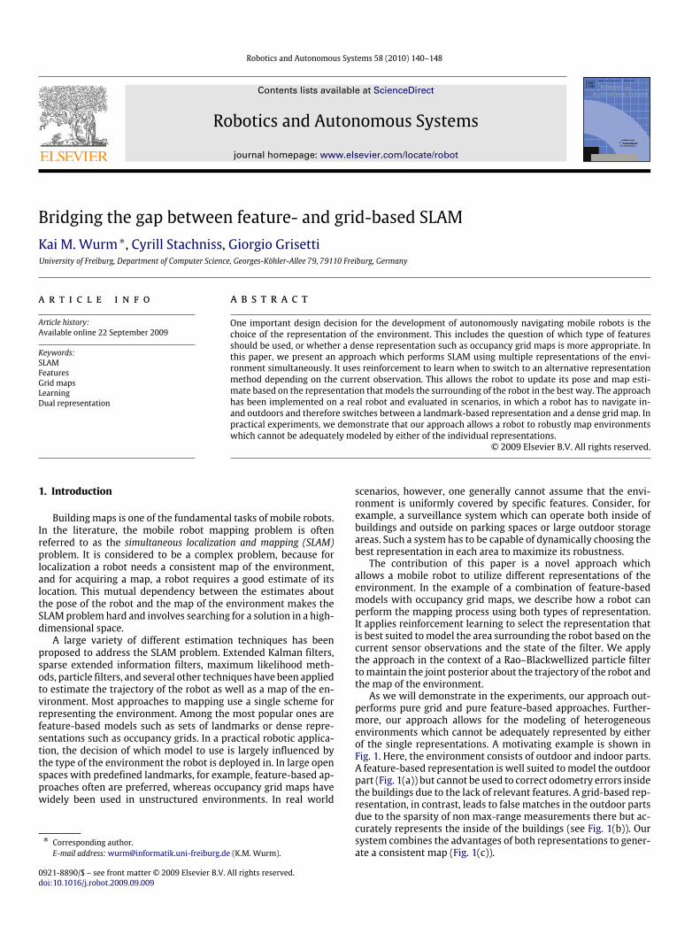
performs pure grid and pure feature-based approaches. Further-more, our approach allows for the modeling of heterogeneousenvironments which cannot be adequately represented by eitherof the single representations. A motivating example is shown inFig. 1. Here, the environment consists of outdoor and indoor parts.A feature-based representation is well suited tomodel the outdoorpart (Fig. 1(a)) but cannot be used to correct odometry errors insidethe buildings due to the lack of relevant features. A grid-based rep-resentation, in contrast, leads to false matches in the outdoor partsdue to the sparsity of non max-range measurements there but ac-curately represents the inside of the buildings (see Fig. 1(b)). Oursystem combines the advantages of both representations to gener-ate a consistent map (Fig. 1(c)).

http://www.elsevier.com/locate/robot

http://www.elsevier.com/locate/robot

mailto:[email protected]

http://dx.doi.org/10.1016/j.robot.2009.09.009

K.M. Wurm et al. / Robotics and Autonomous Systems 58 (2010) 140–148 141

(a) Feature-based mapping system (no features inside the buildings). Features are illustrated by circles.

(b) Grid-based mapping system (few structural information outside).

(c) Combining features and grid maps.

Fig. 1. When mapping environments that contain large open spaces with few landmarks as well as dense structures, a combination of feature maps and grids mapsoutperforms the individual techniques.

This paper is organized as follows. After a discussion of relatedwork, we briefly introduce the SLAM approach utilized in thispaper, namely Rao–Blackwellized particle filters, in Section 3.Whereas Section 4 presents our approach for mapping with a dualrepresentation of the environment, Section 5 explains our modelselection technique based on reinforcement learning. Finally, wepresent experimental results obtained in simulation and on realrobots in Section 6.

2. Related work

Mapping techniques for mobile robots can be roughly classifiedaccording to the map representation and the underlying estima-tion technique. One popular map representation is the occupancygrid [1]. Whereas such grid-based approaches are computationallyexpensive and typically require a huge amount of memory, theyare able to represent arbitrary objects. It should be noted that tocorrect the robot pose estimate a certain amount of obstacles inthe range of the robot’s sensor is needed. This can be a problem ifthe range of the sensor is short as is the case with small scale laserscanners or if the environment is a large open area.Feature-based representations are attractive because of their

compactness. This is a clear advantage in terms of memoryconsumption and processing speed. However, such systems rely onpredefined feature extractors, which assume that some structuresin the environments are known in advance. This clearly limits thefield of action of a robot.The model of the environment and the applied state estimation

technique are often coupled. One of the most popular approachesare extended Kalman filters (EKFs) in combinationwith predefined

landmarks. The effectiveness of the EKF approaches results fromthe fact that they estimate a fully correlated posterior aboutlandmark maps and robot poses [2,3]. Their weakness lies in thestrong assumptions that have to bemade on both the robotmotionmodel and the sensor noise. Moreover, the landmarks are assumedto be uniquely identifiable. There exist techniques [4] to deal withunknown data association in the SLAM context, however, if theseassumptions are violated, the filter is likely to diverge [5–7].Thrun et al. [8] proposed a method that uses the inverse of the

covariance matrix. The advantage of the sparse extended infor-mation filters (SEIFs) is that they make use of the approximativesparsity of the informationmatrix and in thisway can performpre-dictions and updates in constant time. Eustice et al. [9] presenteda technique to make use of exactly sparse information matrices ina delayed-state framework.In a work by Murphy, Doucet, and colleagues [10,11], Rao–

Blackwellized particle filters (RBPF) have been introduced as aneffective means to solve the SLAM problem. Each particle in aRBPF represents a possible trajectory of the robot and a map ofthe environment. The framework has been subsequently extendedby Montemerlo et al. [12,13] for approaching the SLAM problemwith landmarkmaps. To learn accurate gridmaps, RBPFs have beenused by Eliazar and Parr [14] and Hähnel et al. [15]. Whereas thefirst work describes an efficient map representation, the secondpresents an improved motion model that reduces the number ofrequired particles. The work of Grisetti et al. [16] describes animproved variant of the algorithm proposed by Hähnel et al. [15]combined with the ideas of FastSLAM2 [12]. Instead of using afixed proposal distribution, the algorithm computes an improvedGaussian proposal distribution on a per-particle basis on the

142 K.M. Wurm et al. / Robotics and Autonomous Systems 58 (2010) 140–148

fly. A further extension of this method which overcomes thelimitation of the Gaussian assumption has recently been presentedby Stachniss et al. [17]. Additional improvements concerning bothruntime andmemory requirements have been achieved by Grisettiet al. [18] by reusing already computed proposal distributions.So far, there exist only very few methods that try to combine

feature-based models with grid maps. One is the hybrid metricmap (HYMM) approach [19]. It estimates the location of featuresand performs a triangulation between them. In this triangulation,a so called dense map is maintained which can be transformedaccording to the update of the corresponding landmarks. Thisallows the robot to obtain a dense map by using a feature-basedmapping approach. However, it is still required that the robot isable to reliably extract landmarks.A hybrid map is also used in [20]. Sim et al. propose a vision-

based SLAMsystemwhich extracts 3Dpoint landmarks fromstereocamera images. In addition to themap of landmarks, an occupancygrid map is constructed which is used for safe navigation of therobot. In contrast to the approach described in this paper, theSLAM-system is only using the feature map for pose estimation,while the gridmap is used for path planning in an exploration task.A similar approach is described by Makarenko et al. [21]. Here, andecision-theoretic exploration algorithm is described which usesa feature map for SLAM and maintains a grid map to determineknown and unknown regions of the environment. However, thegrid map is not used to correct the estimate of the robot’s pose.Another combination of grid and feature maps has been proposedby Ho and Newman [22]. They use grid maps and visual features ina SLAM system. While the grid map generated from laser scans isused for pose estimation, visual features are used to improve thedetection of loop closures.

3. Mapping with Rao–Blackwellized particle filters

According toMurphy [11], the key idea of theRao–Blackwellizedparticle filter for SLAM is to estimate the joint posterior p(x1:t ,m |z1:t , u1:t−1) about the map m and the trajectory x1:t = x1, . . . , xtof the robot. This estimation is performed given the observationsz1:t = z1, . . . , zt and the odometry measurements u1:t−1 =u1, . . . , ut−1 obtained by the mobile robot. The Rao–Blackwellizedparticle filter for SLAMmakes use of the following factorization

p(x1:t ,m | z1:t , u1:t−1) = p(m | x1:t , z1:t) · p(x1:t | z1:t , u1:t−1). (1)

This factorization allows us to first estimate only the trajectory ofthe robot and then to compute the map given that trajectory. Thistechnique is often referred to as Rao–Blackwellization.Typically, Eq. (1) can be calculated efficiently since the posterior

about maps p(m | x1:t , z1:t) can be computed analytically using‘‘mapping with known poses’’ [1] since x1:t and z1:t are known.To estimate the posterior p(x1:t | z1:t , u1:t−1) about the potential

trajectories, one can apply a particle filter. Each particle representsa potential trajectory of the robot. Furthermore, an individualmap is associated with each sample. The maps are built fromthe observations and the trajectory hypothesis represented by thecorresponding particle.This framework allows a robot to learn models of the environ-

ment and estimate its trajectory, but it leaves open how the en-vironment is represented. So far, this approach has been appliedusing feature-based models [12,13] or grid maps [14,16,15,11].Each representation has its advantages and one typically needssome prior information about the environment to select the appro-priate model. In this paper, we combine both types of maps to rep-resent the environment. This allows us to combine the advantagesof both worlds. Depending on the most recent observation, therobot selects that model which is likely to be the best model in thecurrent situation. In case the environment suggests the use of onesingle model, the result is the same as using the original approach.

4. Dual model of the environment

Our mapping system applies such a Rao–Blackwellized parti-cle filter to maintain the joint posterior about the trajectory of therobot and themap of the environment. In contrast to previous algo-rithms, each particle carries a gridmap aswell as amap of features.The key idea is to maintain both representations simultaneouslyand to select in each step the model that is best suited to updatethe pose and map estimate of the robot. Our approach is indepen-dent of the actual features that are used. In our current system, weuse a laser range finder and extract clusters of beam end pointswhich are surrounded by free space. In thisway,we obtain featuresfrom trees, street lamps, etc. Note that other feature detectors canbe transparently integrated into our approach. The detector itselfis completely transparent to the algorithm.In each step, our algorithm considers the current estimate as

well as the current sensor and odometry observation to select ei-ther the grid or the feature model to perform the next update step.This decision affects the proposal distribution in the particle filterused for mapping. The proposal distribution is used to obtain thenext generation of particles as well as to compute the importanceweights of the samples.In the remainder of this section, we first introduce the charac-

teristics of our particle filter. We then explain in the subsequentsection how to actually select the model for the current step.If the grid map is to be used, we draw the new particle poses

from an improved proposal distribution as introduced by Grisettiet al. [16]. This proposal performs scan-matching on a per particlebasis and then approximates the likelihood function by a Gaussian.This technique has been shown to yield accurate grid maps of theenvironment, given that there is enough structure to perform scan-matching for an initial estimate.When using feature maps, we apply the proposal distribution

as done by Montemerlo et al. [13] in the FastSLAM algorithm. Foreach particle s(i)t−1 in the current particle set a new hypothesis ofthe robot’s pose is generated by sampling from the probabilisticmotion model:

s(i)t ∼ p(st | ut , s(i)t−1). (2)

After the proposal is used to obtain the next generation of sam-ples, the importance weights are computed according to Grisettiet al. [16] and Montemerlo et al. [13] respectively. Note that wecompute for each sample i twoweightsw(i)g (based on the gridmap)andw(i)f (based on the feature map). For resampling, one weight isrequired but we need both values in our decision process as ex-plained in the following Section 5.To carry out the resampling step, we apply the adaptive re-

sampling strategy originally proposed by Doucet [23]. It computesthe so-called effective sample size or effective number of particles(Neff) to decide whether to resample or not. This is done based onthe weights resulting from the proposal used to obtain this gener-ation of samples.

5. Model selection

Probably the most important aspect of our proposed algorithmis to decide which representation to choose given the current sen-sor readings and the filter. In the following, we describe differentstrategies we investigated and which are evaluated in the experi-mental section of this paper.

5.1. Observation likelihood criterion

Amapping approach that relies on scan-matching is most likelyto fail if laser readings cannot be aligned to the map generated


so far. For example, this will probably be the case in large openspacewith sparse observations. In such a situation it is often betterto use a pre-defined feature extractor (in case there are feature) toestimate the pose of the robot.A measure that can be used to detect such a situation is the

observation likelihood that scan-matching seeks to maximize

l(zt , xt ,mg,t) = maxxtp(zt | xt ,mg,t). (3)

To point-wise evaluate the observation likelihood of a laserobservation, we use the so called ‘‘beam endpoint model’’ [24]. Inthis model, the individual beams within a scan are considered tobe independent. The likelihood of a beam is computed based on thedistance between the endpoint of the beamand the closest obstaclein the map from that point.Calculating the average likelihood for all particles results in a

value that can be used as a heuristic to decide which map repre-sentation to use in a given situation:

l =1N

∑i

l(zt , x(i)t ,m

(i)g,t). (4)

A heuristic for selecting the feature-based representation insteadof the grid map can be obtained based on a threshold (l ≤ c1).However, care has to be taken when choosing c1. If this thresh-

old is not chosen optimally the feature map might be used evenif it offers no advantage over the grid map. This will increase thelikelihood of a poor state estimate and therefore of inconsistenciesin the map.

5.2. Neff criterion

As described above, each particle i carries two weights w(i)gand w(i)f , one for the grid-map and one for the feature-map. Theseweights can be seen as an indicator of howwell a particle explainsthe data and therefore can be also used as a heuristic for modelselection. Since the weights of a particle are based on differenttypes of measurement, they cannot be compared directly. Whatcan be compared, however, is the weight distribution over thefilter.One way to measure this difference in the individual weights is

to compute the variance of the weights. Intuitively a set of weightswith low variance does not strongly favor any of the hypothesisrepresented by the particles, while a high variance indicates thatsome hypotheses are more likely than others.This suggests that a strategy based on the Neff value, which is

strongly related to the variance of the weights, can be a reasonableheuristic. Neff is computed for both sets of weights as

Ngeff =1

N∑i=1(w

(i)g )2

and N feff =1

N∑i=1(w

(i)f )2

. (5)

It can be easily seen, that a higher variance in the weights yieldsa lower Neff value. Assuming that a set of particles with a highervariance in the weights is usually more discriminative, it seemsreasonable to switch to the feature-based model whenever N feff <Ngeff.In our experiments, this heuristic generally led to good results.

Nevertheless, there are two aspects which have to be considered.Firstly the variance in particles weights usually does not change

abruptly but gradually. For this reason, the Neff criterion mightfail to indicate the optimal point in time to switch the activelyused representation. This will most notably happen at junctionsbetween areas where one is best modeled using grid maps and theother is best modeled using feature maps. Note that such a behav-ior can also be advantageous, for example in case of false featuredetections.

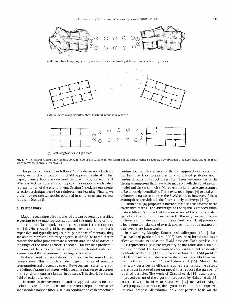
Algorithm 1 The SARSA AlgorithmInitialize Q (s, a) arbitrarilyfor all episodes doinitialize schoose a from s using policy derived from Qrepeattake action a, observe r, s′choose a′ from s′ using policy derived from QQ (s, a) = Q (s, a)+ α[r + γQ (s′, a′)− Q (s, a)]s = s′; a = a′

until s is a terminal stateend for

A second problem arises from the fact that frequent resamplingin a particle filter can lead to particle depletion [23]. Since ourimplementation uses adaptive resampling based on the Neff value,choosing the representationwith the lowerNeff will in general alsolead to more frequent resampling actions.

5.3. Reinforcement learning for model selection

Both approaches described above are clearly heuristics. In thissection,we describe how to use reinforcement learning to combinethe strengths of both heuristics while avoiding their pitfalls. Thebasic idea of reinforcement learning is to find a mapping fromstates S to actions Awhich maximizes a numerical reward signal r(see [25] for an introduction). Such amapping is called a policy andcan be learned by interacting with the environment. Inspired bythe human learning method of trial and error, this class of learningalgorithms performs a series of actions and analyzes the obtainedreward.There exist a number of algorithms for reinforcement learning.

Depending on the prior knowledge an agent has about its environ-ment some approaches may be more appropriate than others. Forexample, if it can be modeled as an Markov decision process, tech-niques such as policy iteration can be utilized. In case no model ofthe environment is available, Monte Carlo methods or Temporal-Difference Learning (TD learning) can be applied.For our approach, we use the SARSA algorithm [25] which is a

popular algorithm among the TD methods and does not requirea model of the environment. It learns an action-value functionQ (s, a) which assigns a value to state-action pairs. Those valuescan then be used to generate a policy (e.g., choose the action thathas the highest value in a given state). The basic steps are given inAlgorithm 1.To apply this method to our model selection problem, we have

to define the states S, the actions A, and the reward r : S → R.Defining the actions is straight forward as A = {ag , af }, where agdefines the use of the grid map and af the use of the feature map.The state set has to be defined in a way that it represents all

necessary information about the sensor input and the filter tomakea decision. To achieve this, our state consists of the average scanmatching likelihood l, a boolean variable given by N feff < N

geff, and

a boolean variable indicating if a known feature has currently beendetected or not. This results in

S := {l} × {1N feff<Ngeff} × {1feature detected}. (6)

The value of l is divided into (here seven) discrete intervals(0.0–0.15, 0.16–0.3, 0.31–0.45, 0.46–0.6, 0.61–0.75, 0.76–0.9,0.91–1.0), resulting in 7 × 2 × 2 = 28 states. It is importantto keep the number of states small since learning the policyotherwisemay require toomany computational resources, even asa preprocessing step which needs to be executed only once.The policy is learned on simulated data where the true robot

pose x∗t is available in every time step t . We use the weighted


average deviation from the true pose to define our reward-fun-ction. To avoid a punishment that result from wrong decisionsin the past (e.g., a wrong rotation), we only use the deviationaccumulated since the last evaluation step t − 1:

r(st) = r(st−1)−N∑i=1

w(i)t ‖x

(i)t − x

∗

t ‖. (7)

Deviations from the simulated path result in negative rewards.As mentioned in Section 5, each particle stores two weights. Forcalculating the weighted average, we use w(i)g if the last actiontaken was ag andw

(i)f if af was taken.

The environment for learning consists of building-like struc-tures with hallways and an outdoor part that models a set of trees.We recorded a simulated path and executed 1000 runs of the learn-ing algorithm. During learning, we us an ε-greedy policy. In states, a greedy policy chooses the action awhich has the highest valueQ (s, a). In contrast to this, an ε-greedy policy allows exploratoryactions by choosing a random action with likelihood ε.More exploration usually facilitates faster learning, so a value

of ε = 0.6 was used in our learning experiments. The learning rateα was set to a fixed value of 0.001, the discounting factor γ wasset to 0.9, which are standard values and led to good results in ourexperiments.This technique results in a policy that tells the robot when to

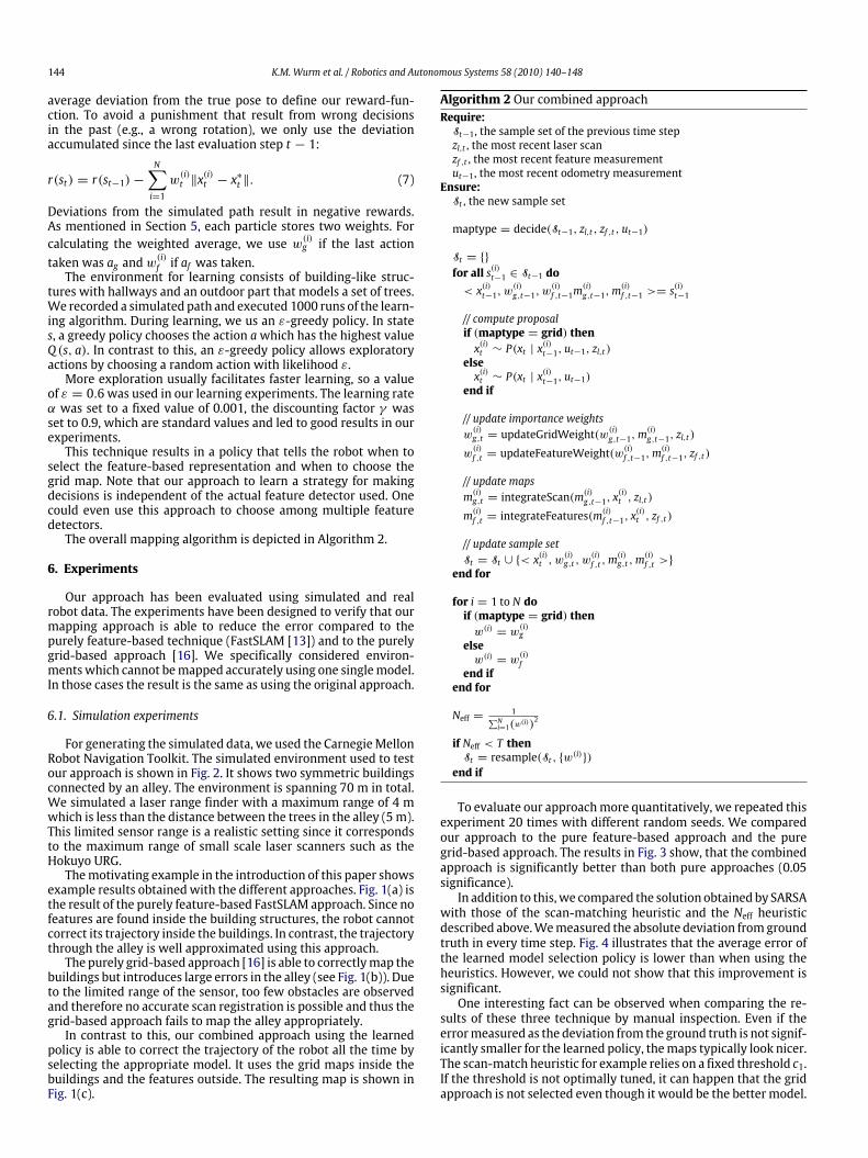
select the feature-based representation and when to choose thegrid map. Note that our approach to learn a strategy for makingdecisions is independent of the actual feature detector used. Onecould even use this approach to choose among multiple featuredetectors.The overall mapping algorithm is depicted in Algorithm 2.

6. Experiments

Our approach has been evaluated using simulated and realrobot data. The experiments have been designed to verify that ourmapping approach is able to reduce the error compared to thepurely feature-based technique (FastSLAM [13]) and to the purelygrid-based approach [16]. We specifically considered environ-mentswhich cannot bemapped accurately using one singlemodel.In those cases the result is the same as using the original approach.

6.1. Simulation experiments

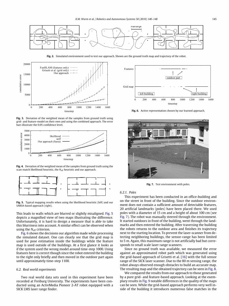
For generating the simulated data, we used the CarnegieMellonRobot Navigation Toolkit. The simulated environment used to testour approach is shown in Fig. 2. It shows two symmetric buildingsconnected by an alley. The environment is spanning 70 m in total.We simulated a laser range finder with a maximum range of 4 mwhich is less than the distance between the trees in the alley (5m).This limited sensor range is a realistic setting since it correspondsto the maximum range of small scale laser scanners such as theHokuyo URG.Themotivating example in the introduction of this paper shows

example results obtainedwith the different approaches. Fig. 1(a) isthe result of the purely feature-based FastSLAM approach. Since nofeatures are found inside the building structures, the robot cannotcorrect its trajectory inside the buildings. In contrast, the trajectorythrough the alley is well approximated using this approach.The purely grid-based approach [16] is able to correctlymap the

buildings but introduces large errors in the alley (see Fig. 1(b)). Dueto the limited range of the sensor, too few obstacles are observedand therefore no accurate scan registration is possible and thus thegrid-based approach fails to map the alley appropriately.In contrast to this, our combined approach using the learned

policy is able to correct the trajectory of the robot all the time byselecting the appropriate model. It uses the grid maps inside thebuildings and the features outside. The resulting map is shown inFig. 1(c).

Algorithm 2 Our combined approachRequire:

St−1, the sample set of the previous time stepzl,t , the most recent laser scanzf ,t , the most recent feature measurementut−1, the most recent odometry measurement

Ensure:St , the new sample set

maptype = decide(St−1, zl,t , zf ,t , ut−1)

St = {}

for all s(i)t−1 ∈ St−1 do< x(i)t−1, w

(i)g,t−1, w

(i)f ,t−1m

(i)g,t−1,m

(i)f ,t−1 >= s

(i)t−1

// compute proposalif (maptype = grid) thenx(i)t ∼ P(xt | x

(i)t−1, ut−1, zl,t)

elsex(i)t ∼ P(xt | x

(i)t−1, ut−1)

end if

// update importance weightsw(i)g,t = updateGridWeight(w

(i)g,t−1,m

(i)g,t−1, zl,t)

w(i)f ,t = updateFeatureWeight(w

(i)f ,t−1,m

(i)f ,t−1, zf ,t)

// update mapsm(i)g,t = integrateScan(m

(i)g,t−1, x

(i)t , zl,t)

m(i)f ,t = integrateFeatures(m(i)f ,t−1, x

(i)t , zf ,t)

// update sample setSt = St ∪ {< x

(i)t , w

(i)g,t , w

(i)f ,t ,m

(i)g,t ,m

(i)f ,t >}

end for

for i = 1 to N doif (maptype = grid) thenw(i) = w

(i)g

elsew(i) = w

(i)f

end ifend for

Neff = 1∑Ni=1(w(i))

2

if Neff < T thenSt = resample(St , {w(i)})

end if

To evaluate our approachmore quantitatively, we repeated thisexperiment 20 times with different random seeds. We comparedour approach to the pure feature-based approach and the puregrid-based approach. The results in Fig. 3 show, that the combinedapproach is significantly better than both pure approaches (0.05significance).In addition to this,we compared the solution obtained by SARSA

with those of the scan-matching heuristic and the Neff heuristicdescribed above.Wemeasured the absolute deviation fromgroundtruth in every time step. Fig. 4 illustrates that the average error ofthe learned model selection policy is lower than when using theheuristics. However, we could not show that this improvement issignificant.One interesting fact can be observed when comparing the re-

sults of these three technique by manual inspection. Even if theerrormeasured as the deviation from the ground truth is not signif-icantly smaller for the learned policy, themaps typically look nicer.The scan-match heuristic for example relies on a fixed threshold c1.If the threshold is not optimally tuned, it can happen that the gridapproach is not selected even though it would be the better model.


Fig. 2. Simulated environment used to test our approach. Shown are the ground truth map and trajectory of the robot.

Fig. 3. Deviation of the weighted mean of the samples from ground truth usinggrid- and feature-model on their own and using the combined approach. The errorbars illustrate the 0.05 confidence level.

Fig. 4. Deviation of the weightedmean of the samples from ground truth using thescan-match likelihood heuristic, the Neff heuristic and our approach.

Fig. 5. Typical mapping results when using the likelihood heuristic (left) and ourSARSA-based approach (right).

This leads to walls which are blurred or slightly misaligned. Fig. 5depicts a magnified view of two maps illustrating the difference.Unfortunately, it is hard to design a measure that is able to takethis blurriness into account. A similar effect can be observed whenusing the Neff criterion.Fig. 6 shows the decisions our algorithmmadewhile processing

the simulated dataset. One can clearly see that the grid map isused for pose estimation inside the buildings while the featuremap is used outside of the buildings. At a first glance it looks asif the system used the wrong model around time-step 1000. Usingfeatures here is correct though since the robot entered the buildingto the right only briefly and then moved in the outdoor part againuntil approximately time-step 1100.

6.2. Real world experiments

Two real world data sets used in this experiment have beenrecorded at Freiburg University. The experiments have been con-ducted using an ActivMedia Pioneer 2-AT robot equipped with aSICK LMS laser range finder.

Fig. 6. Active representation chosen by our learned approach.

Fig. 7. Test environment with poles.

6.2.1. PolesThis experiment has been conducted in an office-building and

on the street in front of the building. Since the outdoor environ-ment does not contain a sufficient amount of detectable features,20 artificial landmarks (poles) have been placed there. We usedpoles with a diameter of 15 cm and a height of about 100 cm (seeFig. 7). The robot was manually steered through the environment.It started outdoors in front of the building, went through the land-marks and then entered the building. After traversing the buildingthe robots returns to the outdoor area and finishes its trajectorynext to the starting location. To prevent the laser-scanner from de-tecting neighboring buildings, the sensor-range has been limitedto 5m. Again, this maximum range is not artificially bad but corre-sponds to small scale laser range scanners.Since no ground truth was available, we measured the error

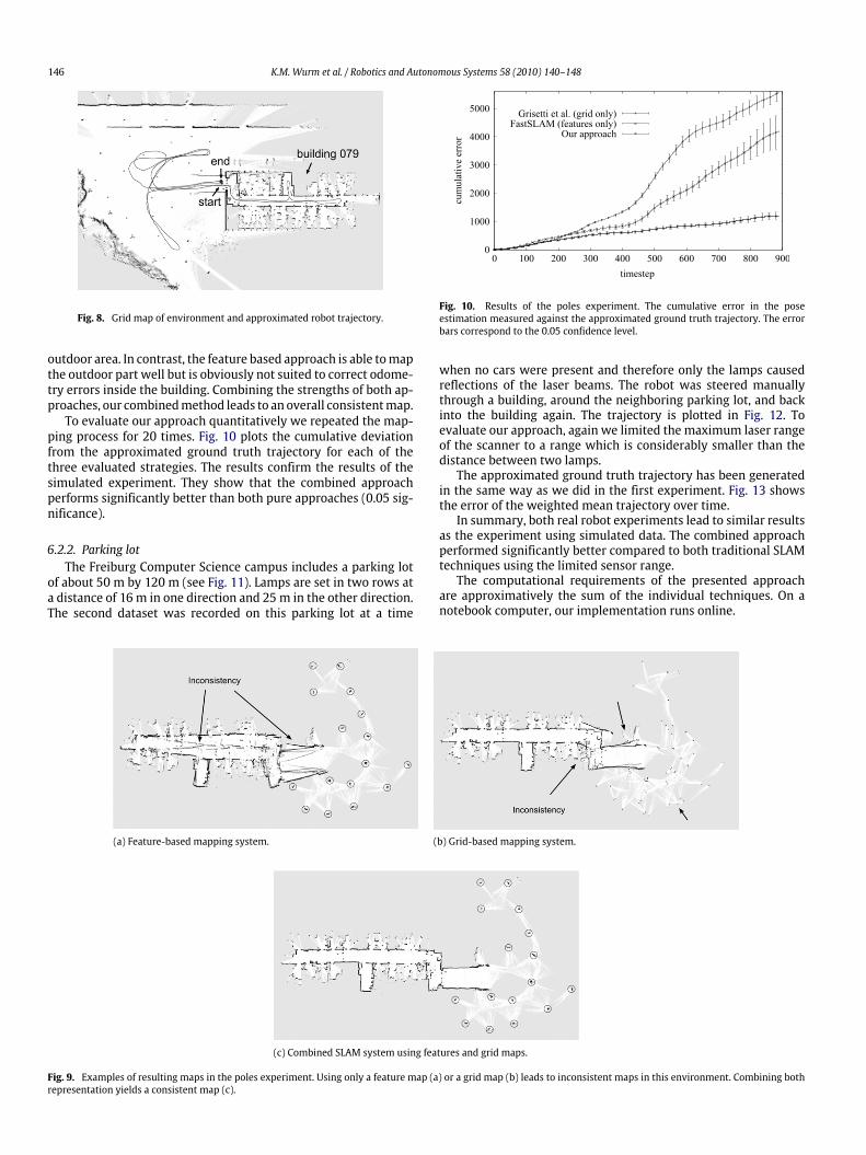
against an approximated robot path which was generated usingthe grid-based approach of Grisetti et al. [16] with the full sensorrange of the SICK laser scanner. Due to the 80 m sensing range, therobot always observed enough obstacles to build an accurate map.The resultingmap and the obtained trajectory can be seen in Fig. 8.We compared the results from our approach to those generated

by a pure grid- and feature-based approach. Looking at the exem-plary results in Fig. 9 notable differences in the quality of the mapscan be seen. While the grid-based approach performs very well in-side of the building it introduces numerous false matches in the


Fig. 8. Grid map of environment and approximated robot trajectory.

outdoor area. In contrast, the feature based approach is able tomapthe outdoor part well but is obviously not suited to correct odome-try errors inside the building. Combining the strengths of both ap-proaches, our combinedmethod leads to an overall consistentmap.To evaluate our approach quantitatively we repeated the map-

ping process for 20 times. Fig. 10 plots the cumulative deviationfrom the approximated ground truth trajectory for each of thethree evaluated strategies. The results confirm the results of thesimulated experiment. They show that the combined approachperforms significantly better than both pure approaches (0.05 sig-nificance).

6.2.2. Parking lotThe Freiburg Computer Science campus includes a parking lot

of about 50 m by 120 m (see Fig. 11). Lamps are set in two rows ata distance of 16 m in one direction and 25m in the other direction.The second dataset was recorded on this parking lot at a time

Fig. 10. Results of the poles experiment. The cumulative error in the poseestimation measured against the approximated ground truth trajectory. The errorbars correspond to the 0.05 confidence level.

when no cars were present and therefore only the lamps causedreflections of the laser beams. The robot was steered manuallythrough a building, around the neighboring parking lot, and backinto the building again. The trajectory is plotted in Fig. 12. Toevaluate our approach, again we limited the maximum laser rangeof the scanner to a range which is considerably smaller than thedistance between two lamps.The approximated ground truth trajectory has been generated

in the same way as we did in the first experiment. Fig. 13 showsthe error of the weighted mean trajectory over time.In summary, both real robot experiments lead to similar results

as the experiment using simulated data. The combined approachperformed significantly better compared to both traditional SLAMtechniques using the limited sensor range.The computational requirements of the presented approach

are approximatively the sum of the individual techniques. On anotebook computer, our implementation runs online.

(a) Feature-based mapping system. (b) Grid-based mapping system.

(c) Combined SLAM system using features and grid maps.

Fig. 9. Examples of resulting maps in the poles experiment. Using only a feature map (a) or a grid map (b) leads to inconsistent maps in this environment. Combining bothrepresentation yields a consistent map (c).


Fig. 11. Parking lot at Freiburg campus.

Fig. 12. Grid map of the parking lot and neighboring building 078 at the Freiburgcampus. The approximated robot trajectory is shown in dark gray, the result of ourcombined mapping approach is shown in light gray.

Fig. 13. Results of the parking lot experiment. Deviation of the weighted mean ofthe samples from the estimated trajectory (using the 80 m range scanner).

7. Conclusions

In this paper, we presented an improved approach to learningmodels of the environment with a Rao–Blackwellized particlefilter. Our approach maintains feature maps as well as grid mapssimultaneously to represent spatial structures. This allows therobot to select the model which provides the best expectedestimates online. The model selection procedure is obtained by areinforcement learning approach. The robot considers the previousestimate as well as the current observations to chose the model

thatwill be used in the upcoming correction step. The process itselfis independent of the actual feature detector. Our approach hasbeen implemented and evaluated on real robot data as well as insimulation experiments. We showed that the presented techniqueallows a robot to more robustly learn maps of different types ofenvironments. It outperforms traditional approaches that use onlyfeatures or only grid maps. In real world experiments, we alsoshowed that our approach is able to map environments whichcould not be modeled by either of the single approaches.

Acknowledgments

This work has partly been supported by the German ResearchFoundation (DFG) under contract number SFB/TR-8 (A3), and bythe EC under contract number FP6-IST-034120-muFly.

References

[1] H.P. Moravec, A.E. Elfes, High resolution maps fromwide angle sonar, in: Proc.of the IEEE Int. Conf. on Robotics & Automation, ICRA, St. Louis, MO, USA 1985,pp. 116–121.

[2] J.J. Leonard, H.F. Durrant-Whyte, Mobile robot localization by trackinggeometric beacons, IEEE Transactions onRobotics andAutomation 7 (4) (1991)376–382.

[3] R. Smith, M. Self, P. Cheeseman, Estimating uncertain spatial realtionships inrobotics, in: I. Cox, G. Wilfong (Eds.), Autonomous Robot Vehicles, SpringerVerlag, 1990, pp. 167–193.

[4] J. Neira, J.D. Tardós, Data association in stochastic mapping using the jointcompatibility test, IEEE Transactions onRobotics andAutomation17 (6) (2001)890–897.

[5] U. Frese, G. Hirzinger, Simultaneous localization and mapping—A discussion,in: Proc. of the IJCAI Workshop on Reasoning with Uncertainty in Robotics,Seattle, WA, USA, 2001, pp. 17–26.

[6] S. Julier, J. Uhlmann, H.F. Durrant-Whyte, A new approach for filteringnonlinear systems, in: Proc. of the American Control Conference, Seattle, WA,USA, 1995, pp. 1628–1632.

[7] J. Uhlmann, Dynamic Map Building and Localization: New TheoreticalFoundations, Ph.D. Thesis, University of Oxford, 1995.

[8] S. Thrun, Y. Liu, D. Koller, A.Y. Ng, Z. Ghahramani, H.F. Durrant-Whyte,Simultaneous localization and mapping with sparse extended informationfilters, Journal of Robotics Research 23 (7/8) (2004) 693–716.

[9] R. Eustice, H. Singh, J.J. Leonard, Exactly sparse delayed-state filters, in: Proc.of the IEEE Int. Conf. on Robotics & Automation, ICRA, Barcelona, Spain, 2005,pp. 2428–2435.

[10] A. Doucet, J.F.G. de Freitas, K. Murphy, S. Russel, Rao–Blackwellized partcilefiltering for dynamic bayesian networks, in: Proc. of the Conf. on Uncertaintyin Artificial Intelligence, UAI, Stanford, CA, USA, 2000, pp. 176–183.

[11] K. Murphy, Bayesian map learning in dynamic environments, in: Proc. of theConf. on Neural Information Processing Systems, NIPS, Denver, CO, USA, 1999,pp. 1015–1021.

[12] M. Montemerlo, S. Thrum, D. Koller, B. Wegbreit, FastSLAM 2.0: An improvedparticle filtering algorithm for simultaneous localization and mapping thatprovably converges, in: Proc. of the Int. Joint Conf. on Artificial Intelligence,IJCAI, 2003, pp. 1151–1156.

[13] M.Montemerlo, S. Thrun, D. Koller, B.Wegbreit, FastSLAM: A factored solutionto simultaneous localization andmapping, in: Proc. of the National Conferenceon Artificial Intelligence, AAAI, Edmonton, Canada, 2002, pp. 593–598.

[14] A. Eliazar, R. Parr, DP-SLAM: Fast, robust simultaneous localization andmapping without predetermined landmarks, in: Proc. of the Int. Joint Conf. onArtificial Intelligence, IJCAI, Acapulco, Mexico, 2003, pp. 1135–1142.

[15] D. Hähnel, W. Burgard, D. Fox, S. Thrun, An efficient FastSLAM algorithmfor generating maps of large-scale cyclic environments from raw laser rangemeasurements, in: Proc. of the IEEE/RSJ Int. Conf. on Intelligent Robots andSystems, IROS, 2003, pp. 206–211.

[16] G. Grisetti, C. Stachniss, W. Burgard, Improved techniques for grid mappingwith Rao–Blackwellized particle filters, IEEE Transactions on Robotics 23 (1)(2007) 34–46.

[17] C. Stachniss, G. Grisetti, W. Burgard, N. Roy, Evaluation of gaussian proposaldistributions for mapping with Rao–Blackwellized particle filters, in: Proc. ofthe IEEE/RSJ International Conference on Intelligent Robots and Systems, IROS,San Diego, CA, USA, 2007.

[18] G. Grisetti, G.D. Tipaldi, C. Stachniss, W. Burgard, D. Nardi, Fast andaccurate slam with Rao–Blackwellized particle filters, Journal of Robotics &Autonomous Systems 55 (1) (2007) 30–38.

[19] E.M. Nebot, J.I. Nieto, J.E. Guivant, The hybrid metric maps (HYMMs): A novelmap representation for denseslam, in: Proc. of the IEEE Int. Conf. on Robotics& Automation, ICRA, 2004.

[20] R. Sim, J.J. Little, Autonomous vision-based exploration and mapping usinghybrid maps and Rao–Blackwellised particle filters, Intelligent Robots andSystems, 2006 IEEE/RSJ International Conference on, October 2006, pp.2082–2089.


[21] A.A. Makarenko, S.B. Williams, F. Bourgoult, H.F. Durrant-Whyte, An experi-ment in integrated exploration, in: Proc. of the IEEE/RSJ Int. Conf. on IntelligentRobots and Systems, IROS, Lausanne, Switzerland, 2002.

[22] K.L. Ho, P.M. Newman, Loop closure detection in slam by combining visual andspatial appearance, Robotics and Autonomous Systems 54 (9) (2006) 740–749.

[23] A. Doucet, On sequential simulation-based methods for bayesian filtering,Technical report, Signal Processing Group, Dept. of Engineering, University ofCambridge, 1998.

[24] S. Thrun, W. Burgard, D. Fox, Probabilistic Robotics, MIT Press, 2005, pp.171–172.

[25] R.S. Sutton, A.G. Barto, Reinforcement Learning: An Introduction, MIT Press,Cambridge, MA, 1998.

Kai M. Wurm is a research scientist at the University ofFreiburg (Germany). He studied computer science at theUniversity of Freiburg and received his diploma degree in2007. His research interests lie in the fields of SLAM,multi-robot exploration, and terrain classification.

Cyrill Stachniss studied computer science at the Univer-sity of Freiburg and received his Ph.D. degree in 2006. Afterhis Ph.D., he was a senior researcher at ETH Zurich. Since2007, he has been an academic advisor at the University ofFreiburg in the Laboratory for Autonomous Intelligent Sys-tems. His research interests lie in the areas of robot navi-gation, exploration, SLAM, as well as learning approaches.

Giorgio Grisetti is working as a Post-doc at the Au-tonomous Intelligent Systems Lab of the University ofFreiburg. Up to 2006, he was a Ph.D. student at Universityof Rome ‘‘La Sapienzia’’ in the Intelligent Systems Lab. Hisadvisor was Daniele Nardi and he received his Ph.D. de-gree in April 2006. His research interests lie in the areasof mobile robotics. His previous and current work aims toprovide effective solutions to mobile robot navigation inall its aspects: SLAM, localization, and path planning.