Boletın de la Asociacion Matematica Venezolana, Vol. XII, No. 1 (2005) 65
Boundary value problems in
complex analysis I
Heinrich Begehr
Abstract
A systematic investigation of basic boundary value problems for com-plex partial differential equations of arbitrary order is started in these lec-tures restricted to model equations. In the first part [3] the Schwarz, theDirichlet, and the Neumann problems are treated for the inhomogeneousCauchy-Riemann equation. The fundamental tools are the Gauss theoremand the Cauchy-Pompeiu representation. The principle of iterating theserepresentation formulas is introduced which will enable treating higherorder equations. Those are studied in a second part of these lectures.
The whole course was delivered at the Simon Bolıvar University inCaracas in May 2004.
1 Introduction
Complex analysis is one of the most influencial areas in mathematics. It hasconsequences in many branches like algebra, algebraic geometry, geometry, num-ber theory, potential theory, differential equations, dynamical systems, integralequations, integral transformations, harmonic analysis, global analysis, oper-ator theory and many others. It also has a lot of applications e.g. in physics.Classical ones are elasticity theory, fluid dynamics, shell theory, underwateracoustics, quantum mechanics etc.In particular the theory of boundary value problems for analytic functions as theRiemann problem of linear conjugacy and the general Riemann-Hilbert problemhas had a lot of influence and even has initiated the theory of singular integralequations and index theory.
Complex analysis is one of the main subjects in university curricula in math-ematics. It is in fact a simply accessible theory with more relations to othersubjects in mathematics than other topics. In complex analysis all structuralconcepts in mathematics are stressed. Algebraic, analytic and topological con-cepts occur and even geometry is involved. Also questions of ordering sets maybe discussed in connection with complex analysis. Gauss, Cauchy, Weierstraßand Riemann were the main initiators of complex analysis and there was more
66 H. Begehr
than a century of rapid development. Nowadays complex analysis is not any-more in the center of mathematicsl research. But there are still activities in thisarea and problems not yet solved. One of these subjects, complex methods forpartial differential equations, will be presented in these lectures.Almost everything in this course is elementary in the sense that the results arejust consequences of the main theorem of culculus in the case of several vari-ables, i.e. of the Gauss divergence theorem. Some nonelementary results will beused as properties of some singular integral operators. They will be just quotedand somebody interested in the background has to consult references given.Everything else is just combinatorics. Hierarchies of differential equations, ofintegral representation formulas, of kernel functions, of Green and Neumannfunctions arise by iterating processes leading from lower to higher order sub-jects. In this sense everything is evident. As Kronecker ones has expressedit, mathematics is the science where everything is evident. The beautiness ofmathematics is partly reflected by esthetic formulas. All this will be seen below.
2 The complex Gauss theorems
In complex analysis it is convenient to use the complex partial differential op-erators ∂z and ∂z defined by the real partial differential operators ∂x and ∂y
as
2∂z = ∂x − i∂y , 2∂z = ∂x + i∂y . (1)
Formally they are deducible by treating
z = x+ iy , z = x− iy , x, y ∈ R ,
as independent variables using the chain rule of differentiation.A complex-valued function w = u + iv given by two real-valued functions uand v of the real variables x and y will be denoted by w(z) although beingrather a function of z and z. In case when w is independent of z in an openset of the complex plane C it is an analytic function. It then is satisfying theCauchy-Riemann system of first order partial differential equations
ux = vy , uy = −vx . (2)
This is equivalent towz = 0 (2′)
as follows from
2∂zw = (∂x + i∂y)(u+ iv) = ∂xu− ∂yv + i(∂xv + ∂yu) . (3)
Boundary value problems in complex analysis I 67
In that case also
2∂zw = (∂x − i∂y)(u+ iv) = ∂xu+ ∂yv + i(∂xv − ∂yu)= 2∂xw = −2i∂yw = 2w′ . (4)
Using these complex derivatives the real Gauss divergence theorem for functionsof two real variables being continuously differentiable in some regular domain,i.e. a bounded domain D with smooth boundary ∂D, and continuous in theclosure D = D ∪ ∂D of D, easily can be given in complex forms.
Gauss Theorem (real form) Let (f, g) ∈ C1(D; R2)∩C(D; R2) be a differen-tiable real vector field in a regular domain D ⊂ R2 then∫
D
(fx(x, y) + gy(x, y))dxdy = −∫
∂D
(f(x, y)dy − g(x, y)dx) . (5)
Remark The two-dimensional area integral on the left-hand side is taken fordiv(f, g) = fx +gy. The boundary integral on the right-hand side is just the onedimensional integral of the dot product of the vector (f, g) with the outwardnormal vector ν = (∂sy,−∂sx) on the boundary ∂D with respect to the arclength parameter s. This Gaus Theorem is the main theorem of calculus in R2.
Gauss Theorems (complex form) Let w ∈ C1(D; C) ∩ C(D; C) in a regulardomain D of the complex plane C then∫
D
wz(z)dxdy =12i
∫∂D
w(z)dz (6)
and ∫D
wz(z)dxdy = − 12i
∫∂D
w(z)dz . (6′)
Proof Using (3) and applying (5) shows
2∫D
wz(z)dxdy =∫D
(ux(z)− vy(z))dxdy + i
∫D
(vx(z) + uy(z))dxdy
= −∫
∂D
(u(z)dy + v(z)dx)− i
∫∂D
(v(z)dy − u(z)dx)
= i
∫∂D
w(z)dz
68 H. Begehr
This is formula (6). Taking complex conjugation and observing
∂zw = ∂zw
and replacing w by w leads to (6′).
Remark Formula (6) contains the Cauchy theorem for analytic functions∫γ
w(z)dz = 0
as particular case. If γ is a simple closed smooth curve and D the inner domainbounded by γ then this integral vanishes as (2′) holds.
3 Cauchy-Pompeiu representation formulas
As from the Cauchy theorem the Cauchy formula is deduced from (6) and (6′)representation formulas can be deduced.
Cauchy-Pompeiu representations Let D ⊂ C be a regular domain andw ∈ C1(D; C) ∩ C(D; C). Then using ζ = ξ + iη for z ∈ D
w(z) =1
2πi
∫∂D
w(ζ)dζ
ζ − z− 1π
∫D
wζ(ζ)dξdη
ζ − z(7)
and
w(z) = − 12πi
∫∂D
w(ζ)dζ
ζ − z− 1π
∫D
wζ(ζ)dξdη
ζ − z(7′)
hold.
Proof Let z0 ∈ D and ε > 0 be so small that
Kε(z0) ⊂ D , Kε(z0) = {z :| z − z0 |< ε} .
Denoting Dε = D \Kε(z0) and applying (6) gives
12i
∫∂Dε
w(ζ)dζ
ζ − z0−
∫Dε
wζ(ζ)dξdη
ζ − z0= 0 .
Introducing polar coordinates∫Kε(z0)
wζ(ζ)dξdη
ζ − z0=
ε∫0
2π∫0
wζ(z0 + teiϕ)e−iϕdϕdt
Boundary value problems in complex analysis I 69
and it is seen that∫D
wζ(ζ)dξdη
ζ − z0=
∫Dε
wζ(ζ)dξdη
ζ − z0+
∫Kε(z0)
wζ(ζ)dξdη
ζ − z0
exists and hence
limε→0
∫Dε
wζ(ζ)dξdη
ζ − z0=
∫D
wζ(ζ)dξdη
ζ − z0.
Once again using polar coordinates∫∂Dε
w(ζ)dζ
ζ − z0=
∫∂D
w(ζ)dζ
ζ − z0−
∫∂Kε(z0)
w(ζ)dζ
ζ − z0,
where ∫∂Kε(z0)
w(ζ)dζ
ζ − z0= i
2π∫0
w(z0 + εeiϕ)dϕ ,
is seen to give
limε→0
∫∂Dε
w(ζ)dζ
ζ − z0=
∫∂D
w(ζ)dζ
ζ − z0− 2πiw(z0) .
This proves (7). Formula (7′) can be either deduced similarly or by complexconjugation as in the preceding proof.
Definition 1 For f ∈ L1(D; C) the integral operator
Tf(z) = − 1π
∫D
f(ζ)dξdη
ζ − z, z ∈ C ,
is called Pompeiu operator.The Pompeiu operator, see [10], is investigated in detail in connection with
the theory of generalized analytic functions in Vekua’s book [12], see also [1].Its differentiability properties are important here in the sequal. For generaliza-tions, see e.g. [2], for application [6, 3].
Theorem 1 If f ∈ L1(D; C) then for all ϕ ∈ C10 (D; C)∫
D
Tf(z)ϕz(z)dxdy +∫D
f(z)ϕ(z)dxdy = 0 (8)
70 H. Begehr
Here C10 (D; C) denotes the set of complex-valued functions in D being continu-
ously differentiable and having compact support in D, i.e. vanishing near theboundary.
Proof From (7) and the fact that the boundary values of ϕ vanish at theboundary
ϕ(z) =1
2πi
∫∂D
ϕ(ζ)dζ
ζ − z− 1π
∫D
ϕζ(ζ)dξdη
ζ − z= (Tϕζ)(z)
follows. Thus interchanging the order of integration∫D
Tf(z)ϕz(z)dxdy = − 1π
∫D
f(ζ)∫D
ϕz(z)dxdy
ζ − zdξdη = −
∫D
f(ζ)ϕ(ζ)dξdη
Formula (8) means that
∂zTf = f (9)
in distributional sense.
Definition 2 Let f, g ∈ L1(D; C). Then f is called generalized (distributional)derivative of g with respect to z if for all ϕ ∈ C1
0 (D; C)∫D
g(z)ϕz(z)dxdy +∫D
f(z)ϕ(z)dxdy = 0 .
This derivative is denoted by f = gz = ∂zg.In the same way generalized derivatives with respect to z are defined. In
case a function is differentiable in the ordinary sense it is also differentiable inthe distributional sense and both derivatives coincide.
Sometimes solutions to differential equations in distributional sense can beshown to be differentiable in the classical sense. Then generalized solutionsbecome classical solutions to the equation. An example is the Cauchy-Riemannsystem (2′), see [12, 1].
More delecate is the differentiation of Tf with respect to z. For z ∈ C \Dobviously Tf is analytic and its derivative
∂zTf(z) = Πf(z) = − 1π
∫D
f(ζ)dξdη
(ζ − z)2. (10)
That this holds in distributional sense also for z ∈ D almost everywhere whenf ∈ Lp(D; C), 1 < p, and the integral on the right-hand side is understood as a
Boundary value problems in complex analysis I 71
Cauchy principal value integral∫D
f(ζ)dξdη
(ζ − z)2= lim
ε→0
∫D\Kε(z)
f(ζ)dξdη
(ζ − z)2
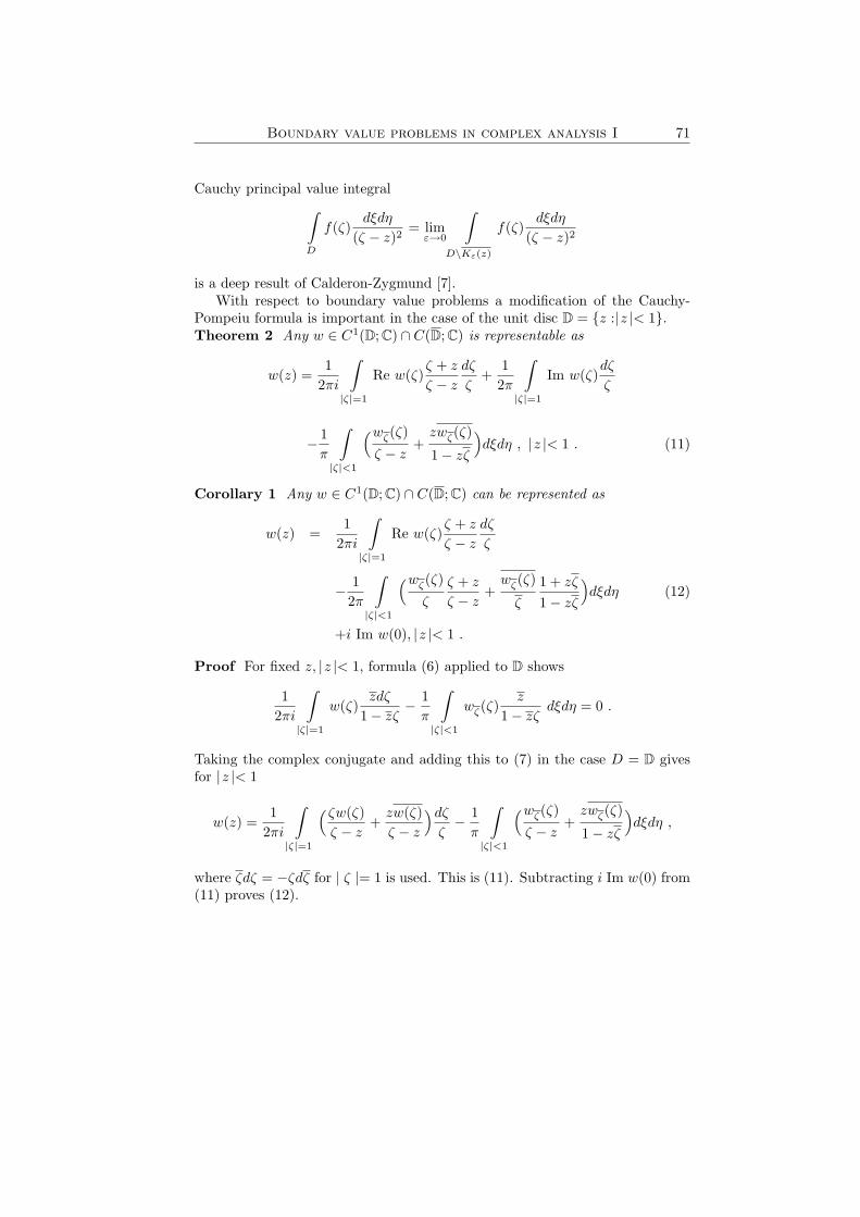
is a deep result of Calderon-Zygmund [7].With respect to boundary value problems a modification of the Cauchy-
Pompeiu formula is important in the case of the unit disc D = {z :|z |< 1}.Theorem 2 Any w ∈ C1(D; C) ∩ C(D; C) is representable as
w(z) =1
2πi
∫|ζ|=1
Re w(ζ)ζ + z
ζ − z
dζ
ζ+
12π
∫|ζ|=1
Im w(ζ)dζ
ζ
− 1π
∫|ζ|<1
(wζ(ζ)ζ − z
+zwζ(ζ)
1− zζ
)dξdη , |z |< 1 . (11)
Corollary 1 Any w ∈ C1(D; C) ∩ C(D; C) can be represented as
w(z) =1
2πi
∫|ζ|=1
Re w(ζ)ζ + z
ζ − z
dζ
ζ
− 12π
∫|ζ|<1
(wζ(ζ)ζ
ζ + z
ζ − z+wζ(ζ)
ζ
1 + zζ
1− zζ
)dξdη (12)
+i Im w(0), |z |< 1 .
Proof For fixed z, |z |< 1, formula (6) applied to D shows
12πi
∫|ζ|=1
w(ζ)zdζ
1− zζ− 1π
∫|ζ|<1
wζ(ζ)z
1− zζdξdη = 0 .
Taking the complex conjugate and adding this to (7) in the case D = D givesfor |z |< 1
w(z) =1
2πi
∫|ζ|=1
(ζw(ζ)ζ − z
+zw(ζ)ζ − z
)dζζ− 1π
∫|ζ|<1
(wζ(ζ)ζ − z
+zwζ(ζ)
1− zζ
)dξdη ,
where ζdζ = −ζdζ for | ζ |= 1 is used. This is (11). Subtracting i Im w(0) from(11) proves (12).
72 H. Begehr
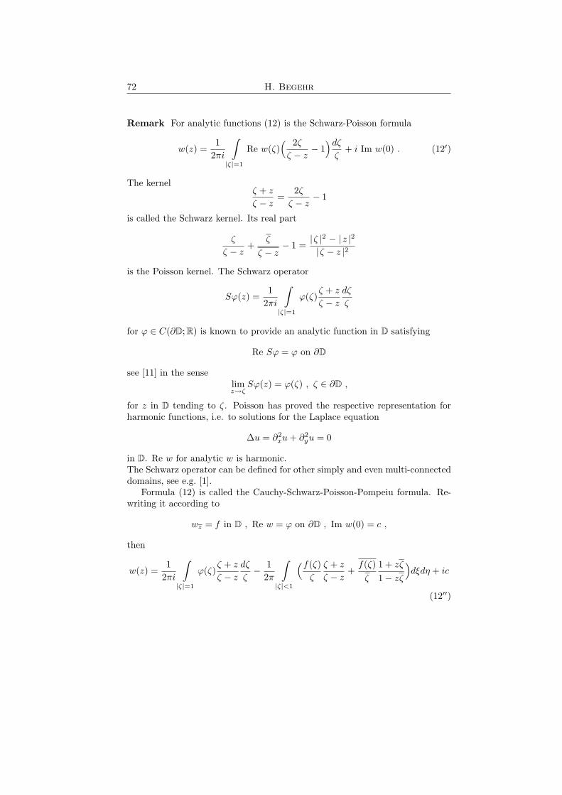
Remark For analytic functions (12) is the Schwarz-Poisson formula
w(z) =1
2πi
∫|ζ|=1
Re w(ζ)( 2ζζ − z
− 1)dζζ
+ i Im w(0) . (12′)
The kernelζ + z
ζ − z=
2ζζ − z
− 1
is called the Schwarz kernel. Its real part
ζ
ζ − z+
ζ
ζ − z− 1 =
|ζ |2 − |z |2
|ζ − z |2
is the Poisson kernel. The Schwarz operator
Sϕ(z) =1
2πi
∫|ζ|=1
ϕ(ζ)ζ + z
ζ − z
dζ
ζ
for ϕ ∈ C(∂D; R) is known to provide an analytic function in D satisfying
Re Sϕ = ϕ on ∂D
see [11] in the senselimz→ζ
Sϕ(z) = ϕ(ζ) , ζ ∈ ∂D ,
for z in D tending to ζ. Poisson has proved the respective representation forharmonic functions, i.e. to solutions for the Laplace equation
∆u = ∂2xu+ ∂2
yu = 0
in D. Re w for analytic w is harmonic.The Schwarz operator can be defined for other simply and even multi-connecteddomains, see e.g. [1].
Formula (12) is called the Cauchy-Schwarz-Poisson-Pompeiu formula. Re-writing it according to
wz = f in D , Re w = ϕ on ∂D , Im w(0) = c ,
then
w(z) =1
2πi
∫|ζ|=1
ϕ(ζ)ζ + z
ζ − z
dζ
ζ− 1
2π
∫|ζ|<1
(f(ζ)ζ
ζ + z
ζ − z+f(ζ)ζ
1 + zζ
1− zζ
)dξdη + ic
(12′′)
Boundary value problems in complex analysis I 73
is expressed by the given data. Applying the result of Schwarz it is easily seenthat taking the real part on the right-hand side and letting z tend to a boundarypoint ζ this tends to ϕ(ζ).Differentiating with respect to z as every term on the right-hand side is analyticbesides the T -operator applied to f this gives f(z). Also for z = 0 besides icall other terms on the right-hand side are real.Hence, (12′′) is a solution to the so-called Dirichlet problem
wz = f in D , Re w = ϕ on ∂D , Im w(0) = c .
This shows how integral representation formulas serve to solve boundaryvalue problems. The method is not restricted to the unit disc but in this casethe solutions to the problems are given in an explicit way.
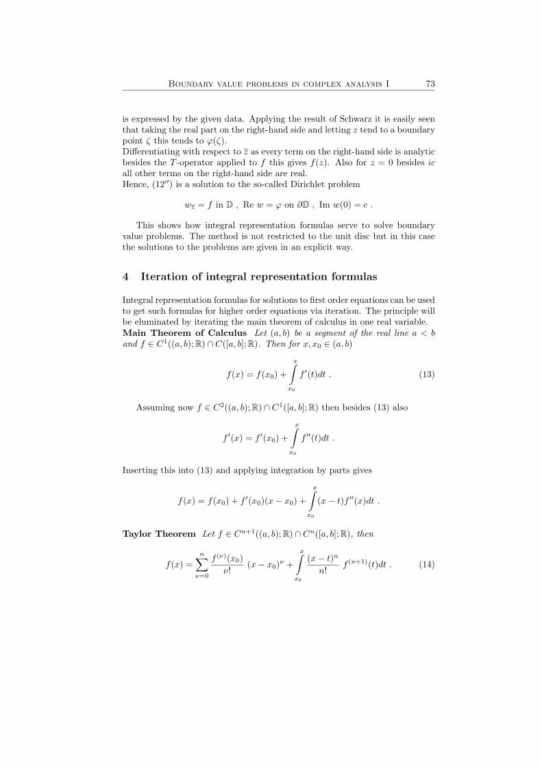
4 Iteration of integral representation formulas
Integral representation formulas for solutions to first order equations can be usedto get such formulas for higher order equations via iteration. The principle willbe eluminated by iterating the main theorem of calculus in one real variable.Main Theorem of Calculus Let (a, b) be a segment of the real line a < band f ∈ C1((a, b); R) ∩ C([a, b]; R). Then for x, x0 ∈ (a, b)
f(x) = f(x0) +
x∫x0
f ′(t)dt . (13)
Assuming now f ∈ C2((a, b); R) ∩ C1([a, b]; R) then besides (13) also
f ′(x) = f ′(x0) +
x∫x0
f ′′(t)dt .
Inserting this into (13) and applying integration by parts gives
f(x) = f(x0) + f ′(x0)(x− x0) +
x∫x0
(x− t)f ′′(x)dt .
Taylor Theorem Let f ∈ Cn+1((a, b); R) ∩ Cn([a, b]; R), then
f(x) =n∑
ν=0
f (ν)(x0)ν!
(x− x0)ν +
x∫x0
(x− t)n
n!f (n+1)(t)dt . (14)
74 H. Begehr
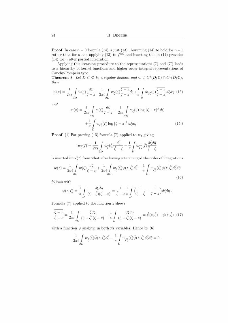
Proof In case n = 0 formula (14) is just (13). Assuming (14) to hold for n− 1rather than for n and applying (13) to f (n) and inserting this in (14) provides(14) for n after partial integration.
Applying this iteration procedure to the representations (7) and (7′) leadsto a hierarchy of kernel functions and higher order integral representations ofCauchy-Pompeiu type.Theorem 3 Let D ⊂ C be a regular domain and w ∈ C2(D; C) ∩ C1(D; C),then
w(z) =1
2πi
∫∂D
w(ζ)dζ
ζ − z− 1
2πi
∫∂D
wζ(ζ)ζ − z
ζ − zdζ+
1π
∫D
wζζ(ζ)ζ − z
ζ − zdξdη (15)
andw(z) =
12πi
∫∂D
w(ζ)dζ
ζ − z+
12πi
∫∂D
wζ(ζ) log |ζ − z |2 dζ
+1π
∫D
wζζ(ζ) log |ζ − z |2 dξdη . (15′)
Proof (1) For proving (15) formula (7) applied to wz giving
wζ(ζ) =1
2πi
∫∂D
wζ(ζ)
dζ
ζ − ζ− 1π
∫D
wζζ
(ζ)dξdη
ζ − ζ
is inserted into (7) from what after having interchanged the order of integrations
w(z) =1
2πi
∫∂D
w(ζ)dζ
ζ − z+
12πi
∫∂D
wζ(ζ)ψ(z, ζ)dζ − 1
π
∫D
wζζ
(ζ)ψ(z, ζ)dξdη
(16)follows with
ψ(z, ζ) =1π
∫D
dξdη
(ζ − ζ)(ζ − z)=
1ζ − z
1π
∫D
( 1ζ − ζ
− 1ζ − z
)dξdη .
Formula (7) applied to the function z shows
ζ − z
ζ − z=
12πi
∫∂D
ζdζ
(ζ − ζ)(ζ − z)− 1π
∫D
dξdη
(ζ − ζ)(ζ − z)= ψ(z, ζ)− ψ(z, ζ) (17)
with a function ψ analytic in both its variables. Hence by (6)
12πi
∫∂D
wζ(ζ)ψ(z, ζ)dζ − 1
π
∫D
wζζ
(ζ)ψ(z, ζ)dξdη = 0 .
Boundary value problems in complex analysis I 75
Subtracting this from (16) and applying (17) gives (15).(2) In order to show (15′) formula (7′) giving
wζ(ζ) = − 12πi
∫∂D
wζ(ζ)
dζ
ζ − ζ− 1π
∫D
wζζ
(ζ)dξdη
ζ − ζ
is inserted in (7) so that after interchanging the order of integrations
w(z) =1
2πi
∫∂D
w(ζ)dζ
ζ − z− 1
2πi
∫∂D
wζ(ζ)Ψ(z, ζ)dζ − 1
π
∫D
wζζ
(ζ)Ψ(z, ζ)dξdη
(18)with
Ψ(z, ζ) =1π
∫D
dξdη
(ζ − ζ)(ζ − z).
The function log | ζ − z |2 is a C1-function in D \ {ζ} for fixed ζ ∈ D. Henceformula (7) may be applied in Dε = D \ {z :| z − ζ |≤ ε} for small enoughpositive ε giving for z ∈ Dε
log | ζ − z |2= 12πi
∫∂Dε
log | ζ − ζ |2 dζ
ζ − z− 1π
∫Dε
1
ζ − ζ
dξdη
ζ − z.
As for ε <|z − ζ |
1π
∫|ζ−ζ|<ε
1
ζ − ζ
dξdη
ζ − z=
1π
ε∫0
2π∫0
eiϕ
ζ − z + teiϕdϕdt
exists and tends to zero with ε tending to zero and because for ε <|z − ζ |
12πi
∫|ζ−ζ|=ε
log | ζ − ζ |2 dζ
ζ − z=
2 log ε2πi
∫|ζ−ζ|=ε
dζ
ζ − z= 0
this relation results in
log | ζ − z |2= 12πi
∫∂D
log | ζ − ζ |2 dζ
ζ − z− 1π
∫D
1
ζ − ζ
dξdη
ζ − z= Ψ(z, ζ)−Ψ(z, ζ)
(19)where the function Ψ is analytic in z but anti-analytic in ζ. Therefore from (6′)
12πi
∫∂D
wζ(ζ)Ψ(z, ζ)dζ +
1π
∫D
wζζ
(ζ)Ψ(z, ζ)dξdη = 0 .
76 H. Begehr
Adding this to (18) and observing (19) proves (15′).Remark There are dual formulas to (15) and (15′) resulting from interchangingthe roles of (7) and (7′) in the preceding procedure. They arise also fromcomplex conjugation of (15) and (15′) after replacing w by w. They are
w(z) = − 12πi
∫∂D
w(ζ)dζ
ζ − z+
12πi
∫∂D
wζ(ζ)ζ − z
ζ − zdζ +
1π
∫D
wζζ(ζ)ζ − z
ζ − zdξdη
(15′′)and
w(z) = − 12πi
∫∂D
w(ζ)dζ
ζ − z− 1
2πi
∫∂D
wζ(ζ) log |ζ − z |2 dζ
+1π
∫D
wζζ(ζ) log |ζ − z |2 dξdη . (15′′′)
The kernel functions (ζ − z)/(ζ − z) , log | ζ − z |2 , (ζ − z)/(ζ − z) of thesecond order differential operators ∂2
z , ∂z∂z, ∂2z respectively are thus obtained
from those Cauchy and anti-Cauchy kernels 1/(ζ − z) and 1/(ζ − z) for theCauchy-Riemann operator ∂z and its complex conjugate ∂z.
Continuing in this way in [4, 5], see also [1], a hierarchy of kernel functionsand related integral operators are constructed and general higher order Cauchy-Pompeiu representation formulas are developed.Definition 3 For m,n ∈ Z satisfying 0 ≤ m+ n and 0 < m2 + n2 let
Km,n(z, ζ)=
(−1)n(−m)!(n− 1)!π
(ζ − z)m−1(ζ − z)n−1 if m ≤ 0 ,
(−1)m(−n)!(m− 1)!π
(ζ − z)m−1(ζ − z)n−1 if n ≤ 0 ,
(ζ − z)m−1(ζ − z)n−1
(m− 1)!(n− 1)!π
[log |ζ − z |2
−m−1∑µ=1
1µ −
n−1∑ν=1
1ν
]if 1 ≤ m,n ,
(20)
and for f ∈ L1(D; C), D ⊂ C a domain,
T0,0f(z) = f(z) for (m,n) = (0, 0) ,
Tm,nf(z) =∫D
Km,n(z, ζ)f(ζ)dξdη for (m,n) 6= (0, 0) . (21)
Boundary value problems in complex analysis I 77
Examples
T0,1f(z) = − 1π
∫D
f(ζ)ζ − z
dξdη , T1,0f(z) = − 1π
∫D
f(ζ)ζ − z
dξdη ,
T0,2f(z) =1π
∫D
f(ζ)ζ − z
ζ − zdξdη , T2,0f(z) =
1π
∫D
f(ζ)ζ − z
ζ − zdξdη,
T1,1f(z) =1π
∫D
f(ζ) log |ζ − z |2 dξdη ,
T−1,1f(z) = − 1π
∫D
f(ζ)(ζ − z)2
dξdη , T1,−1f(z) = − 1π
∫D
f(ζ)(ζ − z)2
dξdη.
The kernel functions are weakly singular as long as 0 < m + n. But form + n = 0, 0 < m2 + n2 they are strongly singular and the related integraloperators are strongly singular of Calderon-Zygmund type to be understood asCauchy principle value integrals. They are useful to solve higher order partialdifferential equations. Km,n turns out to be the fundamental solution to ∂m
z ∂nz
for 0 ≤ m,n. As special cases to the general Cauchy-Pompeiu representationdeduced in [4] two particular situations are considered.Theorem 4 Let w ∈ Cn(D; C) ∩ Cn−1(D; C) for some n ≥ 1. Then
w(z) =n−1∑ν=0
12πi
∫∂D
∂νζw(ζ)
(z − ζ)ν
ν!(ζ − z)dζ − 1
π
∫D
∂nζw(ζ)
(z − ζ)n−1
(n− 1)!(ζ − z)dξdη
(22)This formula obviously is a generalization to (15) and can be proved induct-
ively in the same way as (15).Theorem 5 Let w ∈ C2n(D; C) ∩ C2n−1(D; C) for some n ≥ 1. Then
w(z) =1
2πi
∫∂D
w(ζ)ζ − z
dζ +n−1∑ν=1
12πi
∫∂D
(ζ − z)ν−1(ζ − z)ν
(ν − 1)!ν!
[log |ζ − z |2 −
ν−1∑ρ=1
1ρ−
ν∑σ=1
1σ
](∂ζ∂ζ)
νw(ζ)dζ
(23)
+n∑
ν=1
12πi
∫∂D
|ζ − z |2(ν−1)
(ν − 1)!2[log |ζ − z |2 −2
ν−1∑ρ=1
1ρ
]∂ν−1
ζ ∂νζw(ζ)dζ
+1π
∫D
|ζ − z |2(n−1)
(n− 1)!2[log |ζ − z |2 −2
n−1∑ρ=1
1ρ
](∂ζ∂ζ)
nw(ζ)dξdη .

78 H. Begehr
This representation contains (15′) as a particular case for n = 1. The proofalso follows by induction on the basis of (7) and (7′).
For the general case related to the differential operator ∂mz ∂
nz some particular
notations are needed which are not introduced here, see [5].
5 Basic boundary value problems
As was pointed out in connection with the Schwarz-Poisson formula in the caseof the unit disc boundary value problems can be solved explicitly. For this reasonthis particular domain is considered. This will give necessary information aboutthe nature of the problems considered. The simplest and therefore fundamentalcases occur with respect to analytic functions.Schwarz boundary value problem Find an analytic function w in the unitdisc, i.e. a solution to wz = 0 in D, satisfying
Re w = γ on ∂D , Im w(0) = c
for γ ∈ C(∂D; R), c ∈ R given.Theorem 6 This Schwarz problem is uniquely solvable. The solution is givenby the Schwarz formula
w(z) =1
2πi
∫|ζ|=1
γ(ζ)ζ + z
ζ − z
dζ
ζ+ ic . (24)
The proof follows from the Schwarz-Poisson formula (12′) together with a de-tailed study of the boundary behaviour, see [11].Dirichlet boundary value problem Find an analytic function w in the unitdisc, i.e. a solution to wz = 0 in D, satisfying for given γ ∈ C(∂D; C)
w = γ on ∂D .
Theorem 7 This Dirichlet problem is solvable if and only if for |z |< 1
12πi
∫|ζ|=1
γ(ζ)zdζ
1− zζ= 0 . (25)
The solution is then uniquely given by the Cauchy integral
w(z) =1
2πi
∫|ζ|=1
γ(ζ)dζ
ζ − z. (26)
Remark This result is a consequence of the Plemelj-Sokhotzki formula, seee.g. [9, 8, 1]. The Cauchy integral (26) obviously provides an analytic function
Boundary value problems in complex analysis I 79
in D and one in C \ D, C the Riemann sphere. The Plemelj-Sokhotzki formulastates that for |ζ |= 1
limz→ζ,|z|<1
w(z)− limz→ζ,1<|z|
w(z) = γ(ζ) .
In order that for any |ζ |= 1
limz→ζ,|z|<1
w(z) = γ(ζ)
the conditionlim
z→ζ,1<|z|w(z) = 0
is necessary and sufficient. However, the Plemelj-Sokhotzki formula in its clas-sical formulation holds if γ is Holder continuous. Nevertheless, for the unit discHolder continuity is not needed, see [9].Proof 1. (25) is shown to be necessary. Let w be a solution to the Dirichletproblem. Then w is analytic in D having continuous boundary values
limz→ζ
w(z) = γ(ζ) (27)
for all |ζ |= 1.Consider for 1 <|z | the function
w(1z
)= − 1
2πi
∫|ζ|=1
γ(ζ)zdζ
1− zζ= − 1
2πi
∫|ζ|=1
γ(ζ)z
ζ − z
dζ
ζ.
As with z, 1 <|z |, tending to ζ, |ζ |= 1, 1/z tends to ζ too, limz→ζ w(1/z) exists,i.e. limz→ζ w(z) exists for 1 <|z |. From
w(z)− w(1z
)=
12πi
∫|ζ|=1
γ(ζ)( ζ
ζ − z+
ζ
ζ − z− 1
)dζζ
and the properties of the Poisson kernel for |ζ |= 1
limz→ζ,|z|<1
w(ζ)− limz→ζ,1<|z|
w(z) = γ(ζ) (28)
follows. Comparison with (27) shows limz→ζ w(z) = 0 for 1 <|z |. As w(∞) = 0then the maximum principle for analytic functions tells that w(z) ≡ 0 in 1 <|z |.This is condition (25).2. The sufficiency of (25) follows at once from adding (25) to (26) leading to
w(z) =1
2πi
∫|ζ|=1
γ(ζ)( ζ
ζ − z+
z
ζ − z
)dζζ
=1
2πi
∫|ζ|=1
γ(ζ)( ζ
ζ − z+
ζ
ζ − z− 1
)dζζ.
80 H. Begehr
Thus for |ζ |= 1lim
z→ζ,|z|<1w(z) = γ(ζ)
follows again from the properties of the Poisson kernel.The third basic boundary value problem is based on the outward normal
derivative at the boundary of a regular domain. This directional derivative on acircle |z−a |= r is in the direction of the radius vector, i.e. the outward normalvector is ν = (z − a)/r, and the normal derivative in this direction ν given by
∂ν = ∂r =z
r∂z +
z
r∂z .
In particular for the unit disc D
∂r = z∂z + z∂z .
Neumann boundary value problem Find an analytic function w in theunit disc, i.e. a solution to wz = 0 in D, satisfying for some γ ∈ C(∂D; C) andc ∈ C
∂νw = γ on ∂D , w(0) = c .
Theorem 8 This Neumann problem is solvable if and only if for |z |< 1
12πi
∫|ζ|=1
γ(ζ)dζ
(1− zζ)ζ= 0 (29)
is satisfied. The solution then is
w(z) = c− 12πi
∫|ζ|=1
γ(ζ) log(1− zζ)dζ
ζ. (30)
Proof The boundary condition reduced to the Dirichlet condition
zw′(z) = γ(z) for |z |= 1
because of the analyticity of w. Hence from the preceding result
zw′(z) =1
2πi
∫|ζ|=1
γ(ζ)dζ
ζ − z
if and only if for |z |< 1
12πi
∫|ζ|=1
γ(ζ)zdζ
1− zζ= 0 . (31)
Boundary value problems in complex analysis I 81
But as zw′(z) vanished at the origin this imposes the additional condition
12πi
∫|ζ|=1
γ(ζ)dζ
ζ= 0 (32)
on γ. Then
w′(z) =1
2πi
∫|ζ|=1
γ(ζ)dζ
(ζ − z)ζ.
Integrating shows
w(z) = c− 12πi
∫|ζ|=1
γ(ζ) logζ − z
ζ
dζ
ζ
which is (30). Adding (31) and (32) leads to
12πi
∫|ζ|=1
γ(ζ)1
1− zζ
dζ
ζ=
12πi
∫|ζ|=1
γ(ζ)ζ
ζ − z
dζ
ζ
= − 12πi
∫|ζ|=1
γ(ζ)dζ
ζ − z= 0 ,
i.e. to (29). By integration this gives
12πi
∫|ζ|=1
γ(ζ) log(1− zζ)dζ = 0 .
Next these boundary value problems will be studied for the inhomogeneousCauchy-Riemann equation. Using the T -operator the problems will be reducedto the ones for analytic functions. Here in the case of the Neumann problemit will make a difference if the normal derivative on the boundary or only theeffect of z∂z on the function is prescribed.Theorem 9 The Schwarz problem for the inhomogeneous Cauchy-Riemannequation in the unit disc
wz = f in D , Re w = γ on ∂D , Im w(0) = c
for f ∈ L1(D; C), γ ∈ C(∂D; R), c ∈ R is uniquely solvable by the Cauchy-Schwarz-Pompeiu formula
w(z) =1
2πi
∫|ζ|=1
γ(ζ)ζ + z
ζ − z
dζ
ζ+ ic− 1
2π
∫|ζ|<1
[f(ζ)ζ
ζ + z
ζ − z+f(ζ)ζ
1 + zζ
1− zζ
]dξdη
(33)
82 H. Begehr
This representation (33) follows just from (12) assuming that the solutionw exists. But (33) can easily be justified to be a solution. That this solution isunique follows from Theorem 6.Theorem 10 The Dirichlet problem for the inhomogeneous Cauchy-Riemannequation in the unit disc
wz = f in D , w = γ on ∂D
for f ∈ L1(D; C) and γ ∈ C(∂D; C) is solvable if and only if for |z |< 1
12πi
∫|ζ|=1
γ(ζ)zdζ
1− zζ=
1π
∫|ζ|<1
f(ζ)zdξdη
1− zζ. (34)
The solution then is uniquely given by
w(z) =1
2πi
∫|ζ|=1
γ(ζ)dζ
ζ − z− 1π
∫|ζ|<1
f(ζ)dξdη
ζ − z. (35)
Representation (35) follows from (7) if the problem is solvable. The uniquesolvability is a consequence of Theorem 7. That (35) actually is a solution under(34) follows by observing the properties of the T -operator on one hand and from
w(z) =1
2πi
∫|ζ|=1
γ(ζ)( ζ
ζ − z+
ζ
ζ − z− 1
)dζζ
− 1π
∫|ζ|<1
f(ζ)( 1ζ − z
+z
1− zζ
)dξdη = γ(z)
for |z |= 1 on the other.That (34) is also necessary follows from Theorem 7. Applying condition (25)
to the boundary value of the analytic function w − Tf in D, i.e. to γ − Tf on∂D gives (34) because of
12πi
∫|ζ|=1
1π
∫|ζ|<1
f(ζ)dξdη
ζ − ζ
zdζ
1− zζ=
− 1π
∫|ζ|<1
f(ζ)1
2πi
∫|ζ|=1
z
1− zζ
dζ
ζ − ζdξdη = − 1
π
∫|ζ|=1
f(ζ)z
1− zζdξdη
as is seen from the Cauchy formula.Theorem 11 The Neumann problem for the inhomogeneous Cauchy-Riemannequation in the unit disc
wz = f in D , ∂νw = γ on ∂D , w(0) = c ,
Boundary value problems in complex analysis I 83
for f ∈ Cα(D; C), 0 < α < 1, γ ∈ C(∂D; C), c ∈ C is solvable if and only if for|z |< 1
12πi
∫|ζ|=1
γ(ζ)dζ
(1− zζ)ζ+
12πi
∫|ζ|=1
f(ζ)dζ
1− zζ+
1π
∫|ζ|<1
zf(ζ)(1− zζ)2
dξdη = 0 .
(36)The unique solution then is
w(z) = c− 12πi
∫|ζ|=1
(γ(ζ)− ζf(ζ)) log(1− zζ)dζζ− 1π
∫|ζ|<1
zf(ζ)ζ(ζ − z)
dξdη . (37)
Proof The function ϕ = w − Tf satisfies
ϕz = 0 in D , ∂νϕ = γ − zΠf − zf on ∂D , ϕ(0) = c− Tf(0) .
As the property of the Π-operator, see [12], Chapter 1, §8 and §9, guaranteeΠf ∈ Cα(D; C) for f ∈ Cα(D; C) Theorem 8 shows
ϕ(z) = c− Tf(0)− 12πi
∫|ζ|=1
(γ(ζ)− ζΠf(ζ)− ζf(ζ)) log(1− zζ)dζ
ζ
if and only if
12πi
∫|ζ|=1
(γ(ζ)− ζΠf(ζ)− ζf(ζ))dζ
(1− zζ)ζ= 0 .
From1
2πi
∫|ζ|=1
ζΠf(ζ) log(1− zζ)dζ
ζ=
− 1π
∫|ζ|<1
f(ζ)1
2πi
∫|ζ|=1
log(1− zζ)(ζ − ζ)2
dζdξdη =
1π
∫|ζ|<1
f(ζ)1
2πi
∫|ζ|=1
log(1− zζ)(1− ζζ)2
dζdξdη = 0 ,
and1
2πi
∫|ζ|=1
Πf(ζ)dζ
1− zζ= − 1
π
∫|ζ|<1
f(ζ)12π
∫|ζ|=1
1(ζ − ζ)2
dζ
1− zζdξdη
= − 1π
∫|ζ|<1
f(ζ)∂ζ1
1− zζ|ζ=ζ dξdη = − 1
π
∫|ζ|<1
f(ζ)z
(1− zζ)2dξdη
84 H. Begehr
the result follows.Theorem 12 The problem
wz = f in D , zwz = γ on ∂D , w(0) = c
is solvable for f ∈ Cα(D; C), 0 < α < 1, γ ∈ C(∂D; C), c ∈ C, if and only if
12πi
∫|ζ|=1
γ(ζ)dζ
(1− zζ)ζ+z
π
∫|ζ|<1
f(ζ)dξdη
(1− zζ)2= 0 . (38)
The solution is then uniquely given as
w(z) = c− 12πi
∫|ζ|=1
γ(ζ) log(1− zζ)dζ
ζ− z
π
∫|ζ|<1
f(ζ)dξdη
ζ(ζ − z). (39)
Proof The function ϕ = w − Tf satisfies
ϕz = 0 in D , zϕ′(z) = γ − zΠf on ∂D , ϕ(0) = c− Tf(0) .
Comparing this with the problem in the preceding proof leads to the result.Acknowledgement
The author is very grateful for the hospitality of the Mathematics Departmentof the Simon Bolıvar University. In particular his host, Prof. Dr. CarmenJudith Vanegas has made his visit very interesting and enjoyable.
References
[1] Begehr, H.: Complex analytic methods for partial differential equations.An introductory text. World Scientific, Singapore, 1994.
[2] Begehr, H.: Integral representations in complex, hypercomplex and Cliffordanalysis. Integral Transf. Special Funct. 13 (2002), 223-241.
[3] Begehr, H.: Some boundary value problems for bi-bi-analytic functions.Complex Analysis, Differential Equations and Related Topics. ISAACConf., Yerevan, Armenia, 2002, eds. G. Barsegian et al., Nat. Acad. Sci.Armenia, Yerevan, 2004, 233-253.
[4] Begehr, H., Hile, G. N.: A hierarchy of integral operators. Rocky MountainJ. Math. 27 (1997), 669-706.
[5] Begehr, H., Hile, G. N.: Higher order Cauchy-Pompeiu operator theory forcomplex and hypercomplex analysis. Eds. E. Ramirez de Arellano et al.Contemp. Math. 212 (1998), 41-49.
Boundary value problems in complex analysis I 85
[6] Begehr, H., Kumar, A.: Boundary value problems for bi-polyanalytic func-tions. Preprint, FU Berlin, 2003, Appl. Anal., to appear.
[7] Calderon, A., Zygmund, A.: On the existence of certain singular integrals.Acta Math. 88 (1952), 85-139.
[8] Gakhov, F. D.: Boundary value problems. Pergamon Press, Oxford, 1966.
[9] Muskhelishvili, N. I.: Singular integral equations. Dover, New York, 1992.
[10] Pompeiu, D.: Sur une classe de fonctions d’une variable complexe et surcertaine equations integrales. Rend. Circ. Mat. Palermo 35 (1913), 277-281.
[11] Schwarz, H. A.: Zur Integration der partiellen Differentialgleichung∂2u/∂x2 + ∂2u/∂y2 = 0. J. reine angew. Math. 74 (1872), 218-253.
[12] Vekua, I. N.: Generalized analytic functions. Pergamon Press, Oxford,1962.
Heinrich BegehrI. Math. Inst., FU BerlinArnimallee 314195 Berlin, Germanyemail: [email protected]
Recommended