4
Beamforming Narrowband and Broadband Signals
John E. Piper NSWC
USA
1. Introduction
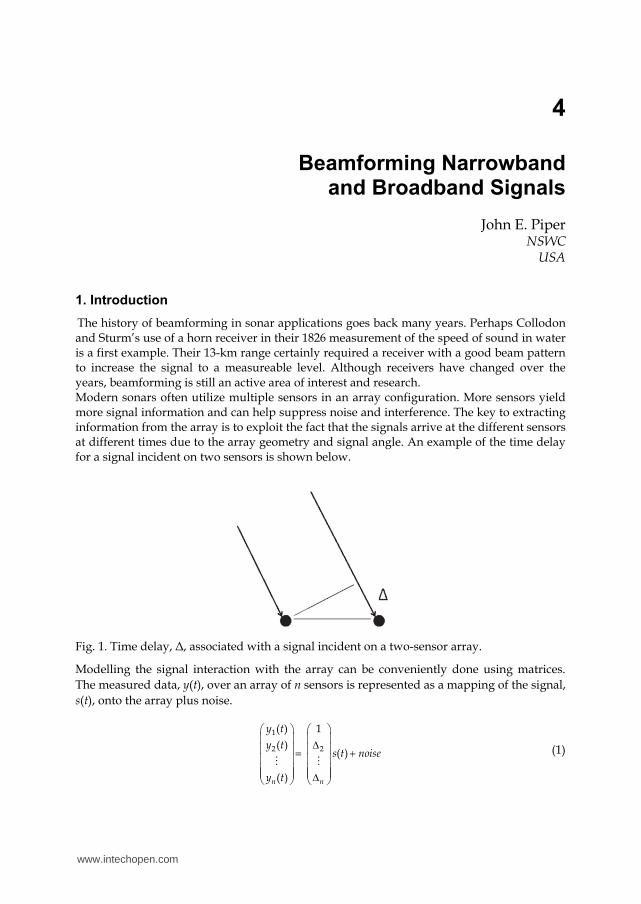
The history of beamforming in sonar applications goes back many years. Perhaps Collodon and Sturm’s use of a horn receiver in their 1826 measurement of the speed of sound in water is a first example. Their 13-km range certainly required a receiver with a good beam pattern to increase the signal to a measureable level. Although receivers have changed over the years, beamforming is still an active area of interest and research. Modern sonars often utilize multiple sensors in an array configuration. More sensors yield more signal information and can help suppress noise and interference. The key to extracting information from the array is to exploit the fact that the signals arrive at the different sensors at different times due to the array geometry and signal angle. An example of the time delay for a signal incident on two sensors is shown below.
Fig. 1. Time delay, Δ, associated with a signal incident on a two-sensor array.
Modelling the signal interaction with the array can be conveniently done using matrices.
The measured data, y(t), over an array of n sensors is represented as a mapping of the signal,
s(t), onto the array plus noise.
1
2 2
( ) 1
( )( )
( )n n
y t
y ts t noise
y t
(1)
www.intechopen.com
Sonar Systems 80
The mapping involves a series of time delays, which are functionally represented by Δ. The signal is referenced to the first array sensor, and the time delays are also referenced to the first array sensor. It is convenient to call this mapping vector, D. The essence of beamforming involves inverting (1) to yield the best estimate of the signal from the measured data. The optimal solution in a least-squares sense can be constructed using the Moore-Penrose inverse. This inverse is well known and widely used in a variety of applications. It is implemented by first left multiplying (1) by the complex transpose of the mapping vector, D†. Then, since D†D is a square matrix (in this case a scalar), left multiplying by (D†D)-1. This allows the best estimate of the signal, s(t), to be expressed in terms of the measured sensor data, y(t), and the mapping vector, D.
1
2† 1 †
( )
( )( ) ( )
( )n
y t
y ts t D D D
y t
(2)
or
† †
1
22
( )
( )1( ) ( 1 )
( )
n
n
y t
y ts t
n
y t
(3)
since,
D†D = n (4)
The mathematical interpretation of (3) corresponds to what is commonly called delay-and-sum beamforming. This equation forms the foundation for beamforming methods. An important observation needs to be noted. The model in (1) was developed for only one
signal. It is the optimal solution for the case that includes only one signal. However, the one-
signal model is often used in multiple-signal environments. Much work has gone into
mitigating the effects of other signals on (3) by introducing weights on the sensors that
reduce the leakage from other directions or can sometimes put a null in the direction of the
interfering signal. However, these methods have their limitations. It is best to use a
multiple-signal model in a multiple-signal environment.
2. Narrowband signals
The required time shifts in the mapping matrix have a particularly simple representation for narrowband signals. This is based on the observation that shifting the phase of a narrowband signal approximates a time shift. The resulting equations allow for high resolution beamforming and direction-of-arrival estimation.
2.1 Phase shift approximation
The extra distance, ∆, that the signal, s, has to travel to the second array element in Fig. 1 is geometrically determined by the distance between the sensors, a, and the angle of incidence, . This extra distance is simply
www.intechopen.com
Beamforming Narrowband and Broadband Signals 81
sin( )a
(5)
For narrowband signals it is convenient to express this distance as the radian measure of the fraction of a wavelength extra distance that the signal travels.
砿 2sin( )a
(6)
This phase angle can then be used to simulate advancing or delaying a narrowband signal
by simple multiplication of the phase term.
結沈釘結沈摘痛 = 結沈岫摘痛袋釘岻 (7)
It should be noted that this is only an approximation in the sense that it does not actually
shift the signal in time. Instead it only changes the phase to match a signal shifted in time.
This phase-shifted signal still starts and stops at the same time samples as the original
signal. So, it is not actually time shifted, but it does approximate a time-shifted signal over
part of its interval. This can be problematic for short signal pulses and large time shifts.
2.2 Narrowband beamforming
The general sonar problem involves multiple sensors and multiple signals. This can be
expressed as a mapping, D, of the m signals onto the n sensors in the array.
1 1
2 2
( ) ( )
( ) ( )
( ) ( )n m
y t s t
y t s tD noise
y t s t
(8)
The narrowband mapping or steering matrix, D, can be expressed in terms of the phase
shifts, φ, associated with the various directions of arrival. Here, each column in the matrix
corresponds to a diffent signal. For a uniform linear array, which is often the case, the
steering matrix has the following Vandermonde stucture.
1 2
1 2 ( 1 )( 1 ) ( 1 )
1 1 1
m
m
ii i
i ni n i n
e e eD
e e e
(9)
Other array geometries can be easily accommodated with this approach by correctly
modeling the various phase delays associated with the various time delays.
Beamforming requires inverting (8). As before, the Moore-Penrose inverse should be used.
This yields the following representation for the signals.
1 1
2 2† 1 †
( ) ( )
( ) ( )( )
( ) ( )m n
s t y t
s t y tD D D
s t y t
(10)
www.intechopen.com
Sonar Systems 82
It is important to note that in this representation the m signals are decoupled or separated. This is generally not the case when conventional beamforming techniques are applied in a multiple signal environment, since conventional beamforming uses a one-signal model that cannot correctly solve the multiple signal case.
It is worthwhile to understand the mathematical details in (10). The term D†y can be thought of as forming m conventional beams from the array data. These beams are then multiplied
by the matrix (D†D)-1 as prescribed by Moore-Penrose. The (D†D)-1 term allows the beams to be be decoupled. This matrix is more fully described in the next section where the importance of the off-diagonal terms in this matrix becomes clear. There is no analog in the
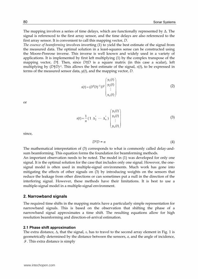
conventional approach since the (D†D)-1 term reduces to a simple scalar in the one-signal model. A simulation example is shown in Fig. 2 for two overlapping narrowband +20 dB signals arriving on a two-sensor array with half-wavelength spacing at incident angles of ±3º. This example simulates a direct signal plus a multipath signal that reflects off the water’s surface and arrives at a slightly later time. The top plot shows the output using simple beam steering. The two signals are not separated since the beamwidth of this approach cannot differentiate signals with small angular separation. The next two plots show the outputs of the Moore-Penrose beamformer directed at +3º and −3º. The two signals are seen to be clearly separated with this approach.
Fig. 2. Simple beam steering and Moore-Penrose beamformer outputs for a two-sensor array with two overlapping narrowband +20 dB signals at ±3º.
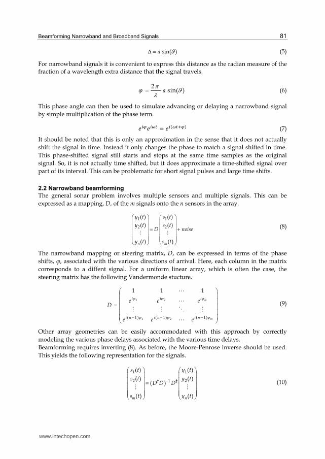
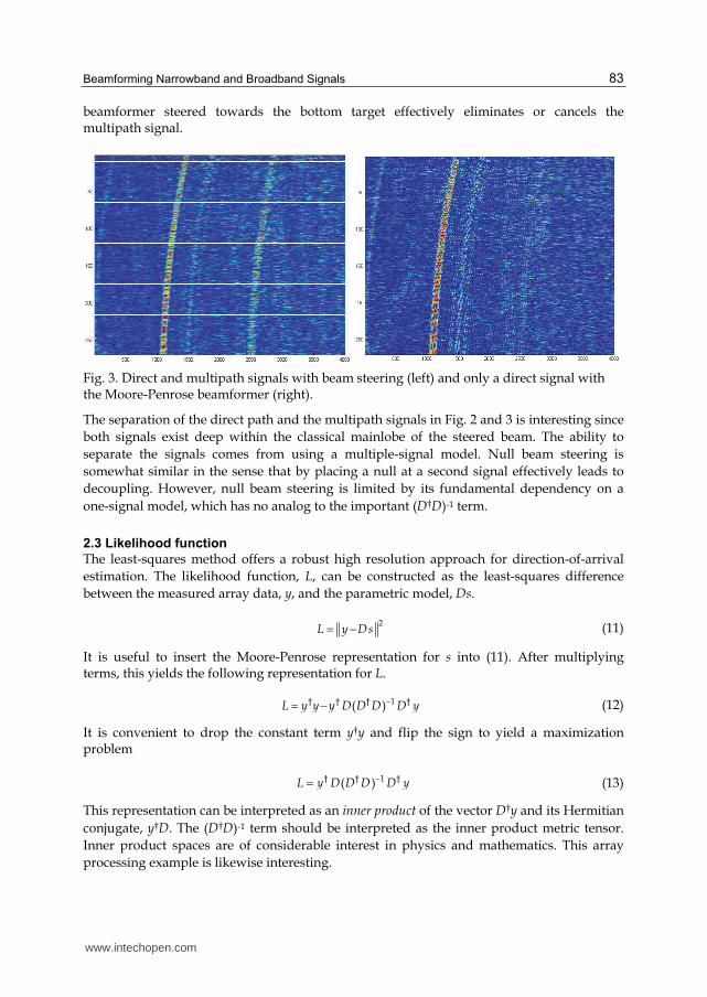
Sonar data was collected with a synthetic aperture rail system at the NSWC test pool. A short 20-kHz narrow beam signal was projected and two vertical wide beam elements received the signal. Fig. 3 shows the results from simple beam steering and from the Moore-Penrose beamformer output. The vertical axis corresponds to the ping number along the rail length, and the horizontal axis corresponds to the relative time sample. The bottom target is clearly seen between time samples 1100 and 1500 in both images. A multipath signal can also be seen between time samples 2500 and 2900 using simple beam steering, since it is within the array’s mainlobe. However, the output from the two-signal Moore-Penrose
www.intechopen.com
Beamforming Narrowband and Broadband Signals 83
beamformer steered towards the bottom target effectively eliminates or cancels the multipath signal.
Fig. 3. Direct and multipath signals with beam steering (left) and only a direct signal with the Moore-Penrose beamformer (right).
The separation of the direct path and the multipath signals in Fig. 2 and 3 is interesting since
both signals exist deep within the classical mainlobe of the steered beam. The ability to
separate the signals comes from using a multiple-signal model. Null beam steering is
somewhat similar in the sense that by placing a null at a second signal effectively leads to
decoupling. However, null beam steering is limited by its fundamental dependency on a
one-signal model, which has no analog to the important (D†D)-1 term.
2.3 Likelihood function
The least-squares method offers a robust high resolution approach for direction-of-arrival
estimation. The likelihood function, L, can be constructed as the least-squares difference
between the measured array data, y, and the parametric model, Ds.
2L y Ds (11)
It is useful to insert the Moore-Penrose representation for s into (11). After multiplying terms, this yields the following representation for L.
† † † 1 †( )L y y y D D D D y (12)
It is convenient to drop the constant term y†y and flip the sign to yield a maximization problem
† † 1 †( )L y D D D D y (13)
This representation can be interpreted as an inner product of the vector D†y and its Hermitian
conjugate, y†D. The (D†D)-1 term should be interpreted as the inner product metric tensor.
Inner product spaces are of considerable interest in physics and mathematics. This array
processing example is likewise interesting.
www.intechopen.com
Sonar Systems 84
It is worthwhile to investigate the properties of this metric tensor for the two-signal and n-element case. The metric tensor is constructed from the steering matrix, D.
11 1 2
2 2
1 2
( 1)†
( 1)
( 1) ( 1)
1 1
1
1
1
1
1
1
i ni i i
i i n
i n i n
i n
i
i n
i
e e e eD D
e e
e e
en
e
en
e
(14)
where 2 1 . The inverse is then
† 1
2
1
1 1( )(1 cos( )) 1(1 cos( )) 1
i n
i
i n
i
en
eD Dn en n
e
(15)
It can be seen that when n is large, the inner product metric tensor tends to become diagonally dominant. In this case the off-diagonal terms tend to be relatively less important, and the conventional signal processing approach starts to assume some validity. The off-diagonal terms in (15) are particularly interesting. These terms are a measure of the coupling between the signals. Interestingly, as the angle between the two signals becomes small, the off-diagonal terms approach the magnitude of the diagonal terms.
0
1
1
i n
i
eLim n
e
(16)
Since the off-diagonal terms can grow to be nearly as large as the diagonal terms when the separation angle is small, they clearly cannot be simply ignored. There are special cases when the off-diagonal terms can be safely ignored. These special
cases occur when the off-diagonal terms are zero, which occur when
2 , 4 , .n (17)
Because the off-diagonal terms are zero at these values, the problem naturally decouples and the signals can be completely separated. These zeros correspond to the zeros commonly seen in conventional sidelobe structures. This is the goal of null steering, which adaptively adds weights to the steering matrix to produce nulls in the beam pattern in the direction of an unwanted signal by exploiting the condition in (17) where the off-diagonal terms go to zero. The likelihood function is commonly expressed using a projection operator and a sample
covariance matrix representation. This may be derived by taking the trace of (13) and
rotating the vector y† to the right side of the equation.
† 1 † †( ( ) )L tr D D D D y y † 1 †( ( ) )tr D D D D R (18)
www.intechopen.com
Beamforming Narrowband and Broadband Signals 85
The least-squares function for the one-signal case reduces to the familiar periodogram
representation, since (D†D)-1 reduces to a simple scalar. The peak in this function corresponds to the best estimate of the parameters.
† 2L D y (19)
2.4 Direction-of-arrival estimation
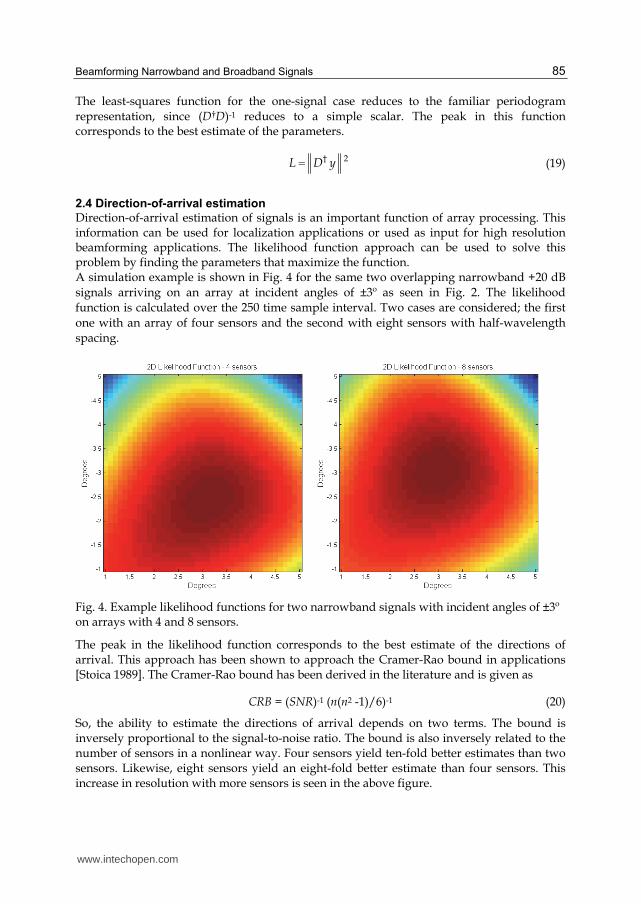
Direction-of-arrival estimation of signals is an important function of array processing. This information can be used for localization applications or used as input for high resolution beamforming applications. The likelihood function approach can be used to solve this problem by finding the parameters that maximize the function. A simulation example is shown in Fig. 4 for the same two overlapping narrowband +20 dB
signals arriving on an array at incident angles of ±3º as seen in Fig. 2. The likelihood
function is calculated over the 250 time sample interval. Two cases are considered; the first
one with an array of four sensors and the second with eight sensors with half-wavelength
spacing.
Fig. 4. Example likelihood functions for two narrowband signals with incident angles of ±3º on arrays with 4 and 8 sensors.
The peak in the likelihood function corresponds to the best estimate of the directions of arrival. This approach has been shown to approach the Cramer-Rao bound in applications [Stoica 1989]. The Cramer-Rao bound has been derived in the literature and is given as
CRB = (SNR)-1 (n(n2 -1)/6)-1 (20)
So, the ability to estimate the directions of arrival depends on two terms. The bound is inversely proportional to the signal-to-noise ratio. The bound is also inversely related to the number of sensors in a nonlinear way. Four sensors yield ten-fold better estimates than two sensors. Likewise, eight sensors yield an eight-fold better estimate than four sensors. This increase in resolution with more sensors is seen in the above figure.
www.intechopen.com
Sonar Systems 86
An alternative and popular approach to direction-of-arrival estimation is the signal subspace method [Schmidt 1986]. This alternative method depends on the eigenvalue structure of the sample covariance matrix. There are a couple of problems with this method. Noise in the sample covariance matrix can lead to poor estimation of the true eigenvalues. Additionally, coherent signals such as seen in multipath lead to problems in the structure of the sample covariance matrix. A number of signal subspace techniques have been developed to address these problems [Wang 1985], [Di Claudio 2001].
2.5 Number of signals resolvable by an array
The number of signals resolvable by an array is somewhat dependent on the array processing methods used. Signal subspace methods are strictly limited to n−1 signals with an array of n sensors [Friedlander 1991]. This limit is imposed since of the n eigenvalues of the sample covariance matrix at least one needs to be assigned to the noise subspace. Hence, that leaves at most n−1 eigenvalues to be assigned to the signal subspace. It may be possible to assign all the eigenvalues to the signal subspace, but then it would technically not be a subspace. Both the Moore-Penrose inverse and the likelihood function require the inversion of the
term D†D. This inverse may or may not exist. In order for it to exist, it is necessary for D†D to be full rank. This requirement constrains the number of resolvable signals. Consider the n by m general steering matrix for n uniformly spaced array elements and m signals. If the incident angles for the incoming signals are all different, then D has m independent columns. For uniformly spaced sensors and most other geometries there are n independent rows. Since the rank of an n by m matrix is less than or equal to min(m,n), D
has full rank if and only if rank(D) = min(m,n). In this case, rank(D†D) = min(m,n), so that
when the incident angles for the incoming angles are distinct, the m by m matrix D†D is invertible if and only if n ≥ m. This result that an n-sensor array can resolve n signals differs from the signal subspace
result of n−1 signals. Simulation and test pool examples of two signals resolved by two
sensors are seen in Fig. 2 and 3. These signals are resolved in the sense that they can be fully
decoupled in beamforming and direction-of-arrival methods.
3. Time-shift operators
Proper array processing requires shifting the signals in time. Time-shift operators, Δ, are useful to translate a digitized signal by an arbitrary amount of time, τ. These can be functionally expressed as
Δ(τ) s(t) = s(t + τ) (21)
Unitary matrix operators can be constructed for this task [Piper 2009]. Although the specific
time-shift matrices developed in this chapter are very useful for solving the general
broadband problem, they have numerous applications in other signal processing problems
[Laakso 1996].
3.1 Unit time shifts
The simplest time-shift operator is the identity matrix, which shifts the time-series signal by
a zero amount. Using matrices with ones along other diagonals, results in time shifts by a
www.intechopen.com

Beamforming Narrowband and Broadband Signals 87
discrete number of time samples. It is worthwhile to consider the unit time-shift operator,
Δ(1). This may be written in a Toeplitz matrix form as
0 1 0 0
0 0 1 0
0 0 0 1(1)
0 0 0 0
(22)
The effect of this operator is to shift vector elements up or backwards in time by one unit. It should be noted that this simple operator is quite independent of the shape of the waveform it operates on. It is convenient to require these operators to be unitary so that inverses are simply complex transposes.
3.2 Fractional time shifts
Construction of the fractional time-shift operator, Δ(τ), for an arbitrary time shift, τ, is best
done in the frequency domain where the fractional time shift can be effected by a phase
shift. This operation can be accomplished by multiplying three matrices; the Fourier matrix,
F, the phase shift matrix, Δ(θ), and the inverse Fourier matrix, F -1. The resultant time-shift
operator can then be functionally written as
( ) ( ) -1F F
(23)
The Fourier, phase shift, and inverse Fourier matrices are listed below
2
2 1
2( 1)2 4
2( 1) ( 1)1
1 1 1 1
1
1
1
N
N
N NN
f f f
f f f
f f f
F
(24)
2
1
1 0 0 0
0 0 0
0 0 0( )
0 0 0 N
p
p
p
(25)
2
( 1)1 2
1 2( 1)2 4
( 1) 2( 1) ( 1)
1 1 1 1
11
1
1
N
N
N N N
f f f
f f fN
f f f
F (26)
www.intechopen.com
Sonar Systems 88
where 2 / 2 /andi N i Nf e p e .
Multiplication of these matrices yields the following exact analytical expression for the fractional time-shift operator
0 1 2 1
1 0 1 2
2 1 0 3
( 1) ( 2) ( 3) 0
( ) .
N
N
N
N N N
(27)
This matrix has a Toeplitz structure. The diagonal terms, Δk, are geometric series and are easily summed.
( 1)2 2 1 11 1(1 )
1
NN kk k N
k k
ppf p f p f
N N pf
(28)
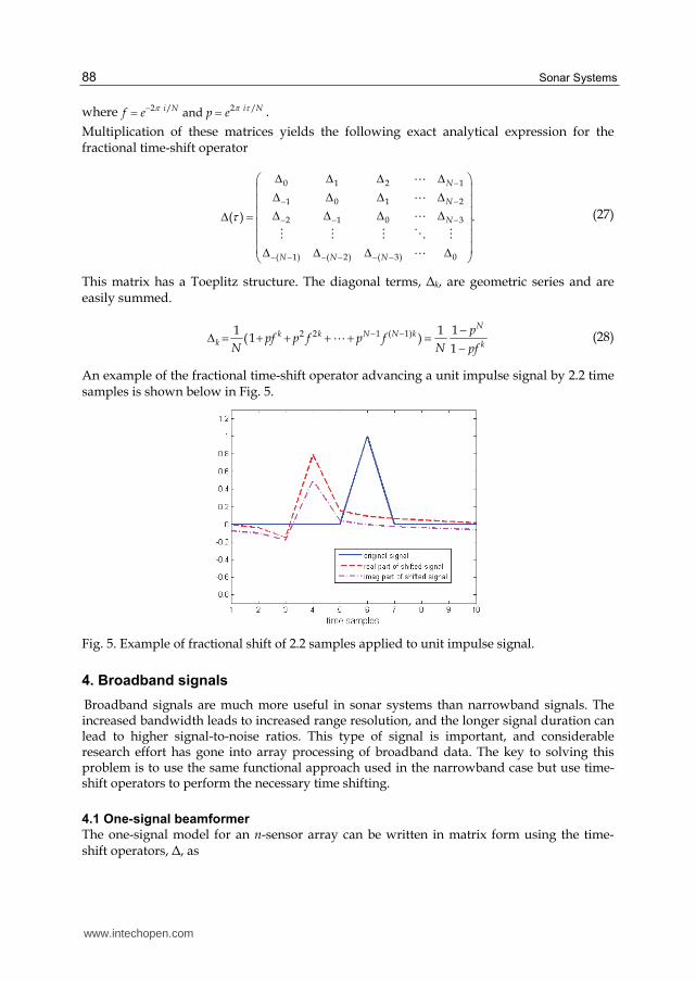
An example of the fractional time-shift operator advancing a unit impulse signal by 2.2 time samples is shown below in Fig. 5.
Fig. 5. Example of fractional shift of 2.2 samples applied to unit impulse signal.
4. Broadband signals
Broadband signals are much more useful in sonar systems than narrowband signals. The increased bandwidth leads to increased range resolution, and the longer signal duration can lead to higher signal-to-noise ratios. This type of signal is important, and considerable research effort has gone into array processing of broadband data. The key to solving this problem is to use the same functional approach used in the narrowband case but use time-shift operators to perform the necessary time shifting.
4.1 One-signal beamformer
The one-signal model for an n-sensor array can be written in matrix form using the time-shift operators, Δ, as
www.intechopen.com
Beamforming Narrowband and Broadband Signals 89
1
2 2
1
n n
y
ys noise
y
(29)
Inversion of this equation in a least-squares sense can be done with the Moore-Penrose
inverse. This representation can be interpreted as a simple delay-and-sum approach.
† †
1
22
1( 1 )n
n
y
ys
n
y
(30)
It is possible and somewhat popular to solve the above problem in the frequency domain.
This can be realized by inserting Fourier transforms and their inverses into (30). Performing
the multiplications reveals that the signal can be constructed in the frequency domain using
simple phase shift operators, Δ(θ), defined in (25). Since the phase-shift operators only have
non-zero elements along the main diagonal, some computational simplicity can be obtained
with this approach.
1
21 † †2
1( 1 ( ) ( ) )n
n
y
ys
n
y
F
FF
F
(31)
4.2 Two-signal beamformer
For two signals and n sensors the sonar model can be written as
1
2 12 22 1
2
1 2
1 1
n n n
y
y snoise
s
y
(32)
The resultant Moore-Penrose inverse solution for the two-signal broadband problem can be functionally written as
11† †
1 12 22 12 2
† †2 22 12 22
1 1
1 1
n
y
s n y
s n
y
(33)
Using the above equation with time-shift operators developed in the previous section leads
to the matrix to be inverted in (33) being rank deficient. This is a problem. It is therefore
necessary to use an approximate inverse. The following equation uses a simple approximate
inverse that allows the signals to be decoupled or separated. However, this approximate
inverse is not well normalized.
www.intechopen.com
Sonar Systems 90
1† †
1 12 22 12 2
† †2 22 12 22
1 ( 1 ) / 11
( 1 ) / 1 1
n
y
s n y
s n n
y
(34)
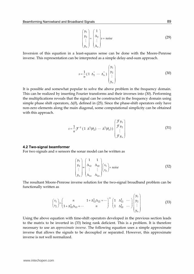
A simulation example of this approach is shown in Fig. 6 for two overlapping +20 dB chirp signals arriving on a two-element array at incident angles of ±3º. This example is similar to the one seen in Fig. 2 in that it also simulates a direct signal plus a delayed multipath signal. The top plot shows the measured signal of sensor 1. The next two plots show the two outputs of the Moore-Penrose beamformer directed at +3º and −3º. The two chirp signals can be seen to be clearly separated with this approach.
Fig. 6. Sensor 1 measured signal and Moore-Penrose beamformer outputs for a two-sensor array with two overlapping broadband +20 dB signals at ±3º.
The two-signal case may be generalized to the multiple-signal case by expanding the signal
vector and steering matrix to account for more signals. The inner product metric term, D†D, will also need to be expanded and an approximate inverse found. For a large number of signals this could be challenging. It may be computationally advantageous to solve this problem in the frequecy domain
instead of the time domain. This can be realized by inserting Fourier transforms and their
inverses into (34) and multiplying to yield the following frequency domain representation.
The Δ(θ) terms are the diagonal phase shift matrices defined in (25).
†1 12 22
†2 22 12
1†
12 2
†22
0 1 ( 1 ( ) ( ) ) /1
0 ( 1 ( ) ( ) ) / 1
1 ( )
1 ( )
n
s n
s n n
y
y
y
-1
-1
F
F
F
F
F
(35)
www.intechopen.com
Beamforming Narrowband and Broadband Signals 91
4.3 Broadband direction-of-arrival estimation
As in the narrowband case, high resolution direction-of-arrival estimates can be obtained using a likelihood function approach. The likelihood function is derived from the least-squares method and is given as
† † 1 †( ) .L y D D D D y (36)
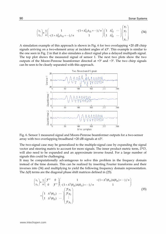
It is again necessary to use an approximate inverse in (36). The best estimate of the angles can be found by numerically evaluating (36) to find its maximum. Two examples are shown in Fig. 7. These correspond to the two chirp signals seen in Fig. 6. These signals have incident angles of ±3º on an array with either 4 or 8 sensors.
Fig. 7. Example likelihood functions for two broadband signals with incident angles of ±3º on arrays with 4 and 8 sensors.
5. Comments
Array beamforming has been largely dominated by one-dimensional thinking. One dimensional in the sense that one-signal models are applied and expected to work in multiple-signal environments. Optimal results can only be expected when the number of signals in the model equals the number of signals in the environment. The Moore-Penrose inverse has been found to be absolutely ideal for beamforming applications in a multiple-signal environment. This inverse is essentially a two-step process. The first step, which is a multiplication by the complex transpose of the steering matrix, D†, can be thought of as simple beamforming. The second step, which is a multiplication by the inner product metric tensor, (D†D)-1, decouples the signals. Time-shift operators allow broadband signals to be beamformed nearly as easily as narrowband signals. A matrix representation of this operation has been given in this chapter. Other approaches are also possible. The motivation for this chapter has been the multipath cancellation problem. This is a significant problem due to the interference of multipath signals that are often seen in sonar data as reflections off the surface and the bottom. Since traditional array processing is
www.intechopen.com
Sonar Systems 92
limited in its abilities to mitigate this problem, it has been necessary to look at what other approaches can be used for this problem. This chapter is a result of that long-term interest and presents a way forward.
6. Acknowledgment
I would like to thank Prof. Henry Unruh for his advice to “make matrices do what you want them to do.” I would also like to thank Dr. Quyen Huynh for his suggestion to use an approximate inverse. I am indebted to Prof. John Bird for pointing out an error in my work. In addition, I would like to acknowledge partial support for this work by the In-Laboratory Independent Research program funded by the Office of Naval Research.
7. References
Stoica, P. & Nehorai, A. (1989). MUSIC, Maximum Likelihood, and the Cramer-Rao Bound, IEEE Transactions on Acoustics, Speech, and Signal Processing, Vol.37, No.5, (May 1989) pp. 720-741, ISSN 0096-3518
Schmidt, R. (1986). Multiple Emitter Location and Signal Estimation, IEEE Transactions on Antennas and Propagation, Vol.34, No.3, (March 1986) pp. 276-280, ISSN 0018-926X
Wang, H. & Kaveh, M. (1985). Coherent Signal-Subspace Processing for the Detection and Estimation of Angles of Arrival of Multiple Wide-band Sources, IEEE Transactions on Acoustics, Speech, and Signal Processing, Vol.33, No.5, (August 1985) pp. 823-831, ISSN 0096-3518
Di Cladio, E. & Parisi, R. (2001). WAVES: Weighted Average of Signal Subspaces for Robust Wideband Direction Finding, IEEE Transactions on Signal Processing, Vol.49, No.10, (October 2001) pp. 2179-2191, ISSN 1053-587X
Friedlander, B. & Weiss, A. (1991). On the Number of Signals Whose Directions can be Estimated by an Array, IEEE Transactions on Signal Processing, Vol.39, No.7, (July 1991) pp. 1686-1689, ISSN 1053-587X
Piper, J. (2009). Exact and Approximate Time-Shift Operators, Proceedings of SPIE Algorithms for Synthetic Aperture Radar Imagery, ISSN: 0277-786X, Vol.7337, Orlando, Florida, USA, April 16-17, 2009
Laafso, T.; Valimaki, V.; Karjalainen, M. & Laine, U. (1996). Splitting the Unit Delay, IEEE Signal Processing Magazine, Vol.13, No.1, (January 1996) pp. 30-60, ISSN 1053-5888
www.intechopen.com
Sonar SystemsEdited by Prof. Nikolai Kolev
ISBN 978-953-307-345-3Hard cover, 322 pagesPublisher InTechPublished online 12, September, 2011Published in print edition September, 2011
InTech EuropeUniversity Campus STeP Ri Slavka Krautzeka 83/A 51000 Rijeka, Croatia Phone: +385 (51) 770 447 Fax: +385 (51) 686 166www.intechopen.com
InTech ChinaUnit 405, Office Block, Hotel Equatorial Shanghai No.65, Yan An Road (West), Shanghai, 200040, China
Phone: +86-21-62489820 Fax: +86-21-62489821
The book is an edited collection of research articles covering the current state of sonar systems, the signalprocessing methods and their applications prepared by experts in the field. The first section is dedicated to thetheory and applications of innovative synthetic aperture, interferometric, multistatic sonars and modeling andsimulation. Special section in the book is dedicated to sonar signal processing methods covering: passivesonar array beamforming, direction of arrival estimation, signal detection and classification using DEMON andLOFAR principles, adaptive matched field signal processing. The image processing techniques include: imagedenoising, detection and classification of artificial mine like objects and application of hidden Markov modeland artificial neural networks for signal classification. The biology applications include the analysis of biosonarcapabilities and underwater sound influence on human hearing. The marine science applications include fishspecies target strength modeling, identification and discrimination from bottom scattering and pelagic biomassneural network estimation methods. Marine geology has place in the book with geomorphological parametersestimation from side scan sonar images. The book will be interesting not only for specialists in the area butalso for readers as a guide in sonar systems principles of operation, signal processing methods and marineapplications.
How to referenceIn order to correctly reference this scholarly work, feel free to copy and paste the following:
John E. Piper (2011). Beamforming Narrowband and Broadband Signals, Sonar Systems, Prof. Nikolai Kolev(Ed.), ISBN: 978-953-307-345-3, InTech, Available from: http://www.intechopen.com/books/sonar-systems/beamforming-narrowband-and-broadband-signals
Recommended