Bag-of-features for category classification
Cordelia Schmid

• Image classification: assigning a class label to the image
Category recognition
Car: presentCow: presentBike: not presentHorse: not present…

• Image classification: assigning a class label to the image
Tasks
Car: presentCow: presentBike: not presentHorse: not present…
• Object localization: define the location and the category
Car CowLocation
Category
Category recognition

Difficulties: within object variations
Variability: Camera position, Illumination,Internal parameters
Within-object variations

Difficulties: within-class variations

• Image classification: assigning a class label to the image
Category recognition
Car: presentCow: presentBike: not presentHorse: not present…
• Supervised scenario: given a set of training images

Image classification• Given
?
Positive training images containing an object class
Negative training images that don’t
A test image as to whether it contains the object class or not• Classify

Bag-of-features for image classification
• Origin: texture recognition• Texture is characterized by the repetition of basic elements or
textons
Julesz, 1981; Cula & Dana, 2001; Leung & Malik 2001; Mori, Belongie & Malik, 2001;Schmid 2001; Varma & Zisserman, 2002, 2003; Lazebnik, Schmid & Ponce, 2003

Texture recognition
Universal texton dictionary
histogram
Julesz, 1981; Cula & Dana, 2001; Leung & Malik 2001; Mori, Belongie & Malik, 2001; Schmid 2001; Varma & Zisserman, 2002, 2003; Lazebnik, Schmid & Ponce, 2003

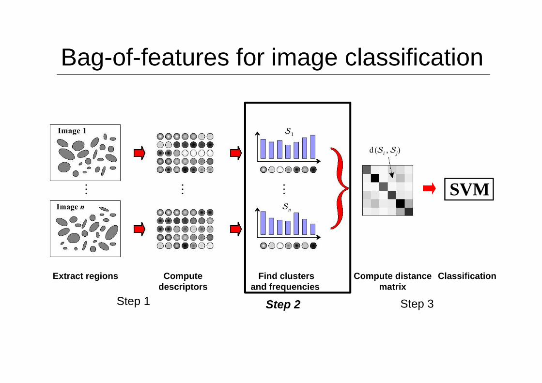
Bag-of-features for image classification
Classification
SVM
Extract regions Compute descriptors
Find clusters and frequencies
Compute distance matrix
[Csurka et al. WS’2004], [Nowak et al. ECCV’06], [Zhang et al. IJCV’07]

Bag-of-features for image classification
Classification
SVM
Extract regions Compute descriptors
Find clusters and frequencies
Compute distance matrix
Step 1 Step 2 Step 3

Step 1: feature extraction
• Scale-invariant image regions + SIFT – Affine invariant regions give “too” much invariance– Rotation invariance for many realistic collections “too” much
invariance
• Dense descriptors – Improve results in the context of categories (for most categories)– Interest points do not necessarily capture “all” features
• Color-based descriptors

Dense features
- Multi-scale dense grid: extraction of small overlapping patches at multiple scales- Computation of the SIFT descriptor for each grid cells- Exp.: Horizontal/vertical step size 3-6 pixel, scaling factor of 1.2 per level
Bag-of-features for image classification
Classification
SVM
Extract regions Compute descriptors
Find clusters and frequencies
Compute distance matrix
Step 1 Step 2 Step 3

Step 2: Quantization
…

Step 2:Quantization
Clustering

Step 2: Quantization
Clustering
Visual vocabulary

Examples for visual words
Airplanes
Motorbikes
Faces
Wild Cats
Leaves
People
Bikes

Step 2: Quantization
• Cluster descriptors– K-means – Gaussian mixture model
• Assign each visual word to a cluster– Hard or soft assignment
• Build frequency histogram

Hard or soft assignment
• K-means hard assignment – Assign to the closest cluster center – Count number of descriptors assigned to a center
• Gaussian mixture model soft assignment– Estimate distance to all centers– Sum over number of descriptors
• Represent image by a frequency histogram

Image representation
…..
frequ
ency
codewords
• each image is represented by a vector, typically 1000-4000 dimension, normalization with L2 norm • fine grained – represent model instances• coarse grained – represent object categories

Bag-of-features for image classification
Classification
SVM
Extract regions Compute descriptors
Find clusters and frequencies
Compute distance matrix
Step 1 Step 2 Step 3
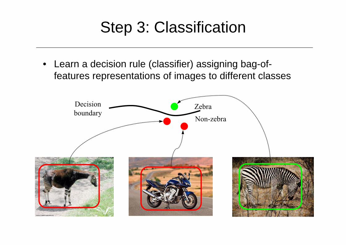
Step 3: Classification
• Learn a decision rule (classifier) assigning bag-of-features representations of images to different classes
Zebra
Non-zebra
Decisionboundary

positive negative
Train classifier,e.g.SVM
Vectors are histograms, one from each training image
Training data

Nearest Neighbor Classifier
• For each test data point : assign label of nearest training data point
• K-nearest neighbors: labels of the k nearest points, vote to classify
• Works well provided there is lots of data and the distance function is good

Linear classifiers• Find linear function (hyperplane) to separate positive and
negative examples
0:negative0:positive
bb
ii
ii
wxxwxx
Which hyperplane is best?Support Vector Machine (SVM)

Kernels for bags of features
• Hellinger kernel
• Histogram intersection kernel
• Generalized Gaussian kernel
• D can be Euclidean distance, χ2 distance etc.
N
i
ihihhhI1
2121 ))(),(min(),(
2
2121 ),(1exp),( hhDA
hhK
N
i ihihihihhhD
1 21
221
21 )()()()(),(2
N
iihihhhK
12121 )()(),(

Multi-class SVMs
• Mutli-class formulations exist, but they are not widely used in practice. It is more common to obtain multi-class SVMs by combining two-class SVMs in various ways.
• One versus all: – Training: learn an SVM for each class versus the others – Testing: apply each SVM to test example and assign to it the
class of the SVM that returns the highest decision value
• One versus one:– Training: learn an SVM for each pair of classes – Testing: each learned SVM “votes” for a class to assign to the test
example

Why does SVM learning work?
• Learns foreground and background visual words
foreground words – high weight
background words – low weight

Localization according to visual word probabilityCorrect − Image: 35
50 100 150 200
20
40
60
80
100
120
Correct − Image: 37
50 100 150 200
20
40
60
80
100
120
Correct − Image: 38
50 100 150 200
20
40
60
80
100
120
Correct − Image: 39
50 100 150 200
20
40
60
80
100
120
foreground word more probable
background word more probable
Illustration

Bag-of-features for image classification
• Excellent results in the presence of background clutter
bikes books building cars people phones trees

Books- misclassified into faces, faces, buildings
Buildings- misclassified into faces, trees, trees
Cars- misclassified into buildings, phones, phones
Examples for misclassified images

Bag of visual words summary
• Advantages:– largely unaffected by position and orientation of object in image– fixed length vector irrespective of number of detections– very successful in classifying images according to the objects they
contain
• Disadvantages:– no explicit use of configuration of visual word positions– poor at localizing objects within an image– no explicit image understanding

Evaluation of image classification (object localization)
• PASCAL VOC [05-12] datasets
• PASCAL VOC 2007– Training and test dataset available– Used to report state-of-the-art results – Collected January 2007 from Flickr– 500 000 images downloaded and random subset selected– 20 classes manually annotated– Class labels per image + bounding boxes– 5011 training images, 4952 test images – Exhaustive annotation with the 20 classes
• Evaluation measure: average precision

PASCAL 2007 dataset
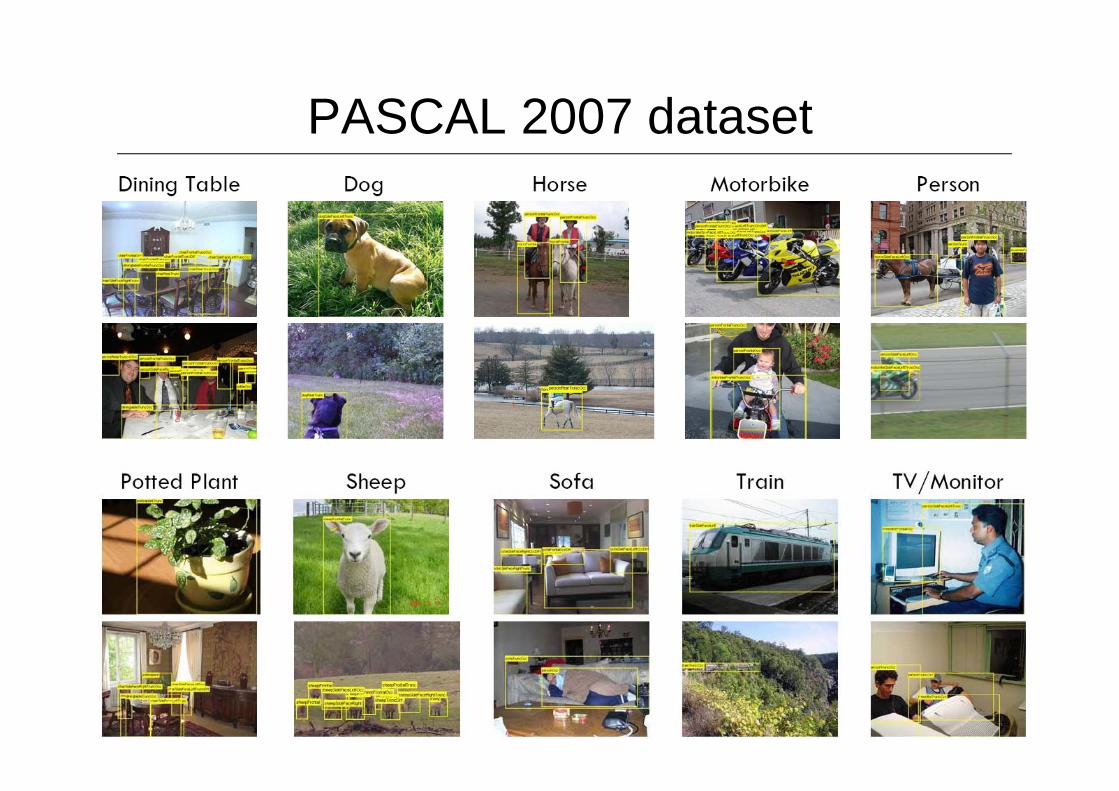
PASCAL 2007 dataset

ImageNet: large-scale image classification dataset
has 14M images from 22k classes
Standard Subsets– ImageNet Large Scale Visual Recognition Challenge 2010 (ILSVRC)
• 1000 classes and 1.4M images– ImageNet10K dataset
• 10184 classes and ~ 9 M images

Evaluation

Results for PASCAL 2007• Winner of PASCAL 2007 [Marszalek et al.] : mAP 59.4
– Combining several channels with non-linear SVM and Gaussian kernel
• Multiple kernel learning [Yang et al. 2009] : mAP 62.2– Combination of several features, Group-based MKL approach
• Object localization & classification [Harzallah et al.’09] : mAP 63.5– Use detection results to improve classification
• Adding objectness boxes [Sanchez at al.’12] : mAP 66.3
• Convolutional Neural Networks [Oquab et al.’14] : mAP 77.7

Spatial pyramid matching
• Add spatial information to the bag-of-features
• Perform matching in 2D image space
[Lazebnik, Schmid & Ponce, CVPR 2006]

Related work
Szummer & Picard (1997) Lowe (1999, 2004) Torralba et al. (2003)
GistSIFT
Similar approaches:Subblock description [Szummer & Picard, 1997]SIFT [Lowe, 1999]GIST [Torralba et al., 2003]

Locally orderless representation at several levels of spatial resolution
level 0
Spatial pyramid representation

Spatial pyramid representation
level 0 level 1
Locally orderless representation at several levels of spatial resolution

Spatial pyramid representation
level 0 level 1 level 2
Locally orderless representation at several levels of spatial resolution

Scene dataset [Labzenik et al.’06]
Suburb Bedroom Kitchen Living room Office
Coast Forest Mountain Open country Highway Inside city Tall building Street
Store Industrial
4385 images15 categories

Scene classification
L Single-level Pyramid
0(1x1) 72.2±0.61(2x2) 77.9±0.6 79.0 ±0.52(4x4) 79.4±0.3 81.1 ±0.33(8x8) 77.2±0.4 80.7 ±0.3

Category classification – CalTech101
L Single-level Pyramid
0(1x1) 41.2±1.21(2x2) 55.9±0.9 57.0 ±0.82(4x4) 63.6±0.9 64.6 ±0.83(8x8) 60.3±0.9 64.6 ±0.7

CalTech101
Easiest and hardest classes
• Sources of difficulty:– Lack of texture– Camouflage– Thin, articulated limbs– Highly deformable shape

Evaluation BoF – spatial
(SH, Lap, MSD) x (SIFT,SIFTC) spatial layout
AP
1 0.53
2x2 0.52
3x1 0.52
1,2x2,3x1 0.54
Image classification results on PASCAL’07 train/val set
Spatial layout not dominant for PASCAL’07 datasetCombination improves average results, i.e., it is appropriate for some classes

Evaluation BoF - spatial
1 3x1Sheep 0.339 0.256
Bird 0.539 0.484
DiningTable 0.455 0.502
Train 0.724 0.745
Image classification results on PASCAL’07 train/val setfor individual categories
Results are category dependent! Combination helps somewhat

Discussion
• Summary– Spatial pyramid representation: appearance of local image
patches + coarse global position information– Substantial improvement over bag of features– Depends on the similarity of image layout
• Recent extensions– Flexible, object-centered grid
• Shape masks [Marszalek’12] => additional annotations – Weakly supervised localization of objects
• [Russakovsky et al.’12, Oquab’14, Cinbis’16]
Recent extensions
• Improved aggregation schemes, such as the Fisher vector, Perronnin et al., ECCV’10 – More discriminative descriptor, power normalization, linear SVM
• ImageNet classification with deep convolutional neural networks, Krizhevsky, Sutskever, Hinton, NIPS 2012

Translated cluster → large derivative on for this
component
Fisher vector
Use a Gaussian Mixture Model as vocabulary Statistical measure of the descriptors of the image w.r.t the GMM Derivative of likelihood w.r.t. GMM parameters
GMM parameters:
weight
mean
co-variance (diagonal)
[Perronnin & Dance 07]

20
35
8
10
Fisher vector image representation
• Mixture of Gaussian/ k-means stores nbr of points per cell
• Fisher vector adds 1st & 2nd order moments– More precise description of regions
assigned to cluster– Fewer clusters needed for same accuracy– Per cluster store: mean and variance of
data in cell– Representation 2D times larger, at same
computational cost– High dimensional, robust representation
20
3
58 10
Fisher vector image representation

Fisher vector image representation

Relation to BOF

Large-scale image classification
• Image classification: assigning a class label to the image
Car: presentCow: presentBike: not presentHorse: not present…
• What makes it large-scale?– number of images– number of classes– dimensionality of descriptor
has 14M images from 22k classes

Current state of the art – image classification
•Deep convolutional neural networks
•Convolutional networks [LeCun’98 …]
•AlexNet [Krizhevsky’12]
•VGGNet [Simonyan’14]
•Google Inception [Szegedy’15]
•ResNet [He’16]
Deep convolutional neural networks
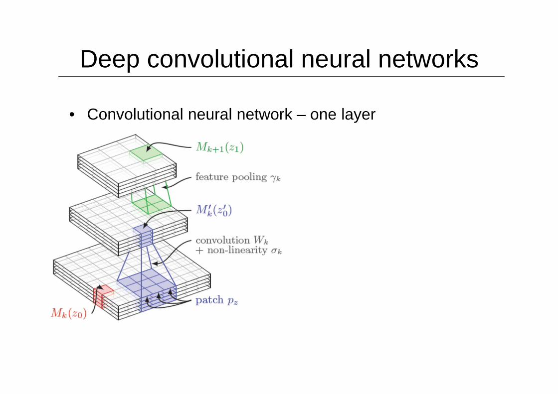
• Convolutional neural network – one layer

Deep convolutional neural networks
• Convolutional neural network – one layer • L
Convolutions:• Learn convolutional filters• Translation invariant• Several filters at each layer• From simple to complex filters

Deep convolutional neural networks
• Convolutional neural network – one layer • L
Non-linearity:• Sigmoid• Rectified linear unit (ReLU)
• Simplifies backpropagation• Makes learning faster• Avoid saturation issues

Deep convolutional neural networks
• Convolutional neural network – one layer • L
Spatial feature pooling:• Average or maximum• Invariance to small
transformations• Larger receptive fields

Deep convolutional neural networks
• First 5 layers: convolutional layer, last 2: full connected• Large model (7 hidden layers, 650k units, 60M parameters)• Requires large training set (ImageNet)• GPU implementation (50x speed up over CPU)
Krizhevsky, Sutskever, Hinton, ImageNet classification with deep convolutional neural networks, NIPS’12

Deep convolutional neural networks
• State of the art result on ImageNet challenge– 1000 categories and 1.2 million images

Visualization of the convolution filters
Zeiler and Fergus, Visualizing and Understanding Convolutional Networks, ECCV’14

Top nine activations
Visualization of the convolution filters
Recommended