Automatically Identifying Lexical Chainsby Means of Statistical Methods—A Knowledge-Free ApproachAutomatisches identifizieren lexikalischer Ketten mittels statistischer Methoden—Ein vorwissensfreier Ansatz
Master-Thesis von Steffen RemusOktober 2012

Automatically Identifying Lexical Chains by Means of Statistical Methods—A Knowledge-Free Approach
Automatisches identifizieren lexikalischer Ketten mittels statistischer Methoden—Ein vorwissensfreier Ansatz
Master-ThesisEingereicht von Steffen Remus
1. Gutachten: Prof. Dr. Chris Biemann2. Gutachten: Dr. Sabine Bartsch
Tag der Einreichung:
Technische Universität DarmstadtDepartment of Computer Science
Ubiquitous Knowledge Processing (UKP) Lab

Erklärung zur Master-Thesis
Hiermit versichere ich die vorliegende Master-Thesis ohne Hilfe Dritter nur mitden angegebenen Quellen und Hilfsmitteln angefertigt zu haben. Alle Stellen, dieaus Quellen entnommen wurden, sind als solche kenntlich gemacht. Diese Arbeithat in gleicher oder ähnlicher Form noch keiner Prüfungsbehörde vorgelegen.
Darmstadt, den 24. Oktober 2012
(S. Remus)

AbstractThe identification of lexical chains is an important building block in modern natural languageprocessing applications such as summarization or text-segmentation. In order to extract lexicalchains it is is necessary to identify the important lexico-semantic relations in a text.
Traditional approaches mostly rely on the use of knowledge resources such as thesauri or lexicaldatabases like WordNet. Hence, the quality of the extracted lexical chains highly depends on thequality and quantity of the entries in the particular knowledge resource. Statistical methods on theother hand have proven to deliver good results in many natural language processing applicationswhere the only prerequisite is a sufficiently large and qualitatively good data collection.
This thesis examines the suitability of statistical methods for the task of identifying lexico-semanticrelations in order to build proper lexical chains. Four algorithms are developed that utilize eitherlatent Dirichlet allocation (LDA) as a probabilistic topic modeling framework or the log-likelihoodratio (LLR) as an indicator for statistically significant co-occurring terms.
An intrinsic evaluation of these algorithms against some trivial and established baseline algorithmsis performed which confirms the hypothesis. For this purpose a secondary issue of this thesis is themanual annotation of lexical chains and the development of a suitable lexical chain comparisonmeasure. Supporting annotation guidelines are developed and an annotation toolkit is adapted inorder to carry out an annotation project where two annotators annotated around 100 documentsfrom the Salsa 2.0 corpus.
Further an extensive survey in the domain of clustering measures is performed in order to find aproper measure for the evaluation of the algorithms as well as for the quantification of the inter-annotator agreement. This measure is finally built of a combination of the adjusted Rand index(ARI) and the normalized basic merge distance (NBMD).
Supplemental material can be found athttp://www.ukp.tu-darmstadt.de/data/lexical-chains-for-german

ZusammenfassungDas Extrahieren von lexikalischen Ketten ist heutzutage ein wichtiger Bestandteil moderner sprach-verarbeitender Applikationen wie z.B. automatische Textzusammenfassung oder Textsegmentie-rung. Das erfolgreiche Extrahieren lexikalischer Ketten setzt die Identifikation von aussagekräfti-gen lexikalisch-semantischen Relationen in einem Text voraus.
Traditionelle Ansätze greifen hierzu auf Wissensressourcen wie Thesauri oder lexikalische Daten-banken zurück. Folglich ist die Qualität der resultierenden lexikalischen Ketten im hohen Ma-ße abhängig von der Qualität und Quantität der Einträge in der Wissensressource. StatistischeMethoden hingegen liefern erwiesenermaßen gute Ergebnisse in vielen sprachverarbeitenden An-wendungsgebieten mit einer hinreichend großen und qualitativ guten Textsammlung als einzigerVoraussetzung.
Diese Arbeit untersucht die Tauglichkeit von statistischen Methoden für die Identifikationlexikalisch-semantischer Relationen und somit lexikalischer Ketten. Vier Algorithmen wurden ent-wickelt welche die Hypothese sinnvoll unterstützen sollen. Diese Algorithmen basieren entwederauf latent Dirichlet allocation (LDA), einem probabilistischem Topic Modeling Framework, oderauf dem log-likelihood ratio (LLR) welches ein Indikator für statistisch signifikante gleichzeitigauftretende Wörter ist.
Die Hypothese wird anhand einer intrinsisch durchgeführten Evaluation bestätigt. Deshalb beschäf-tigt sich diese Arbeit weiterhin mit der manuellen Annotation von lexikalischen Ketten sowie derEntwicklung eines geeigneten Vergleichsmaßes. Annotationsrichtlininen wurden entwickelt undein Annotationsprogramm wurde adaptiert um ein Annotationsprojekt zu unterstützen in demzwei Annotatoren c.a. 100 Dokumente des Salsa 2.0 Korpus annotierten.
Weiterhin wurden diverse Evaluationsmaße der Clustering Domäne ausführlich untersucht umein angemessenes Evaluations- sowie Inter-Annotator Übereinstimmungsmaß auszuwählen. Diesessetzt sich letztendlich aus einer Kombination des adjusted Rand index (ARI) und der normalizedbasic merge distance (NBMD) zusammen.
Zusätzliches Material ist verfügbar unterhttp://www.ukp.tu-darmstadt.de/data/lexical-chains-for-german

AcknowledgmentsI want to sincerely thank Chris for giving me the
opportunity to write this thesis and for being agreat knowledge resource, supervisor, annotator
and motivator in doubtful times. I reallyappreciate all his efforts for guiding
me trough this work.
I also want to thank Richard and Thomas fortheir support and belief in my work.
Next I want to thank all my friends that keptpatient with me while I was struggling so hard.
Meinen Eltern Petra und Peter möchte ichzutiefst dafür danke das sie mich in allen
Lebenslagen unterstützten und immer einoffenes Ohr für mich hatten.
Last but not least I want to express my deepestlove and gratitude to Katrin who was always
there when she was needed most. Sheremembered me to live my life apart
from desk to clear my thoughtsin times they got stuck.

Contents
1. Introduction 11.1. Motivation . . . . . . . . . . . . . . . . . . . . . . . . . . . . . . . . . . . . . . . . . . . . . 21.2. Hypothesis . . . . . . . . . . . . . . . . . . . . . . . . . . . . . . . . . . . . . . . . . . . . . 31.3. Outlook . . . . . . . . . . . . . . . . . . . . . . . . . . . . . . . . . . . . . . . . . . . . . . . 3
2. Lexical Chains 52.1. The Conception of Cohesion . . . . . . . . . . . . . . . . . . . . . . . . . . . . . . . . . . 52.2. Lexical Chain Extraction Algorithms . . . . . . . . . . . . . . . . . . . . . . . . . . . . . . 92.3. Desiderata for Lexical Chain Annotation . . . . . . . . . . . . . . . . . . . . . . . . . . . 19
3. Comparing Lexical Chains 213.1. Clustering Defintion . . . . . . . . . . . . . . . . . . . . . . . . . . . . . . . . . . . . . . . 243.2. Lexical Chains as Clusters . . . . . . . . . . . . . . . . . . . . . . . . . . . . . . . . . . . . 243.3. Comparing Clusterings . . . . . . . . . . . . . . . . . . . . . . . . . . . . . . . . . . . . . . 26
3.3.1. Cluster Conformation . . . . . . . . . . . . . . . . . . . . . . . . . . . . . . . . . . 263.3.2. Desirable Properties . . . . . . . . . . . . . . . . . . . . . . . . . . . . . . . . . . . 26
3.4. Clustering Comparison Measures . . . . . . . . . . . . . . . . . . . . . . . . . . . . . . . 303.4.1. Contingency table . . . . . . . . . . . . . . . . . . . . . . . . . . . . . . . . . . . . 303.4.2. Set based comparison . . . . . . . . . . . . . . . . . . . . . . . . . . . . . . . . . . 303.4.3. Pairwise element comparison . . . . . . . . . . . . . . . . . . . . . . . . . . . . . 323.4.4. Information theory based comparison . . . . . . . . . . . . . . . . . . . . . . . . 343.4.5. B3 . . . . . . . . . . . . . . . . . . . . . . . . . . . . . . . . . . . . . . . . . . . . . . 383.4.6. Edit distance comparison . . . . . . . . . . . . . . . . . . . . . . . . . . . . . . . . 39
3.5. Combining Measures . . . . . . . . . . . . . . . . . . . . . . . . . . . . . . . . . . . . . . . 42
4. Annotating Lexical Chains 454.1. Corpus . . . . . . . . . . . . . . . . . . . . . . . . . . . . . . . . . . . . . . . . . . . . . . . . 454.2. Annotation Scheme . . . . . . . . . . . . . . . . . . . . . . . . . . . . . . . . . . . . . . . . 474.3. Annotation Toolkit . . . . . . . . . . . . . . . . . . . . . . . . . . . . . . . . . . . . . . . . 484.4. Lexical Chain Analysis . . . . . . . . . . . . . . . . . . . . . . . . . . . . . . . . . . . . . . 50
5. Statistical Methods for Lexical Chaining 53
5.1. Candidate Lexical Items . . . . . . . . . . . . . . . . . . . . . . . . . . . . . . . . . . . . . 535.2. Probabilistic Topic Models . . . . . . . . . . . . . . . . . . . . . . . . . . . . . . . . . . . . 53
5.2.1. LDA Mode Method (LDA-MM) . . . . . . . . . . . . . . . . . . . . . . . . . . . . . 585.2.2. LDA Graph Method (LDA-GM) . . . . . . . . . . . . . . . . . . . . . . . . . . . . 595.2.3. LDA Top-N Method (LDA-TM) . . . . . . . . . . . . . . . . . . . . . . . . . . . . . 62
5.3. Term Co-Occurrence Significance . . . . . . . . . . . . . . . . . . . . . . . . . . . . . . . 655.4. Final Notes . . . . . . . . . . . . . . . . . . . . . . . . . . . . . . . . . . . . . . . . . . . . . 67
6. Empirical Analysis 696.1. Corpus . . . . . . . . . . . . . . . . . . . . . . . . . . . . . . . . . . . . . . . . . . . . . . . . 696.2. Experimental Setup . . . . . . . . . . . . . . . . . . . . . . . . . . . . . . . . . . . . . . . . 706.3. Model Selection . . . . . . . . . . . . . . . . . . . . . . . . . . . . . . . . . . . . . . . . . . 716.4. Evaluation . . . . . . . . . . . . . . . . . . . . . . . . . . . . . . . . . . . . . . . . . . . . . 73
7. Summary & Conclusion 797.1. Conclusion . . . . . . . . . . . . . . . . . . . . . . . . . . . . . . . . . . . . . . . . . . . . . 797.2. Future Divisions & Applications . . . . . . . . . . . . . . . . . . . . . . . . . . . . . . . . 807.3. Summary . . . . . . . . . . . . . . . . . . . . . . . . . . . . . . . . . . . . . . . . . . . . . . 81
List of Figures 83
List of Listings 85
List of Tables 87
Bibliography 89
A. Proof: Equality of NMI and V 97
B. Annotation Guidelines 99
C. Annotation Guidelines Companion 111
Contents
1 IntroductionThe hunger of humanity for information is endless. If it is for work, school, or private interest,we seek for information nearly every minute. But the human processing of the enormous mass ofinformation which is entailed in large collections of unstructured text like the World Wide Web issimply impossible. Even the amount of new or changing information that comes in every day oreven every hour is tremendously large. The reliable support by computer systems is indispensablenowadays.
While some information is processable well in an automatic way due to its structuredness likecartographic data or the like, other is still embedded in written or spoken text. It is a major partof modern natural language processing research to computationally understand a text and extractstructured from unstructured data.
A text that is understandable by its nature exhibits an underlying structure which makes the textcoherent; that is, the structure is responsible for making the text “hang” together (Halliday andHasan 1976). The theoretic foundation of this structure is defined as coherence and cohesion. Whilethe former is concerned with the meaning of a text, the latter can be seen as a collection of devicesfor creating it. Cohesion and coherence build the basis for most of the current natural languageprocessing problems that deal with text understanding simply because a natural precondition is acoherent and cohesive text.
Currently only cohesion qualifies for the automatic analysis due to the processing of text withoutthe need of considering the situational environment. Different tasks in natural language processingrequire either explicit or implicit analysis of different cohesive features. For example co-referenceresolution is typically addressed by the analysis of the cohesive devices of reference and substitutionwhile the problem of e.g. word sense disambiguation is typically addressed by the cohesive devicesof lexical cohesion.
Lexical cohesion ties together words or phrases that are semantically related. For example the words“book” and “novel” are related because “book” is a hypernym of “novel”. Though, the automaticanalysis is a tough problem that involves not only the identification of a semantic relation butalso the disambiguation of multiple possible relations and thus the weighting of some kind ofsignificance for the current text. For example, is the word “novel” related to “thesis” because theyare both kinds of writing?—the answer depends on the overall purpose of the text.
Once all the cohesive ties are identified the involved items can be grouped together to form so-called lexical chains. For example when having a cohesive tie involving the words “car” and “tire”
1
and another tie involving the words “car” and “brake” we can build a lexical chain containing thewords “car”, “tire”, and “brake” because they form a cohesively connected unit. By doing so, lexicalchains contain only expressions that refer to the same concept or topic.
Lexical chains thus form a theoretically well founded building block in various natural languageprocessing applications. They are used for example in word sense disambiguation (Okumura andHonda 1994), summarization (Barzilay and Elhadad 1997), malapropism detection & correction(Hirst and St-Onge 1998), document hyperlinking (Green 1996), text segmentation (Stokes et al.2004), topic tracking (Carthy 2004), and many more. Here, the performance of the individual taskmainly depends on the quality of the identified lexical chains.
1.1 Motivation
Current approaches mainly focus on the use of knowledge resources like lexical semantic databases(Hirst and St-Onge 1998) or thesauri (Morris and Hirst 1991) as background information in orderto resolve possible semantic relations for the use of lexical chaining. This strategy has some seriousdrawbacks:
1. The quality of lexical chains highly depends on the quality of the resource. This includes thenumber of terms or phrases that are included in the database as well as the number and thekind of relations between those entries.
2. Resources may be of low quality for rare registers or special domains like the biomedicaldomain or even for resource-scarce languages like Swahili.
3. The use of certain resources may be limited due to policy restrictions or the resource may beonly available online which reduces the computational efficiency.
4. The structure of specific resources may limit the connectivity between certain kinds of items.E.g. lexical databases relate terms based on grammatical features like synonymy and groupthem by their part-of-speech. Grammatical relations across different parts-of-speech occurmuch less frequently than relations within the same part-of-speech and also the number ofrelations for nouns is much higher than for any other part-of-speech. Hence many algorithmsthat use lexical databases limit their search scope to nouns only.
5. The costs-benefit ratio for manually compiling such a resource is unbalanced; the costs aresimply too expensive.
Hence the choice of the resource has a direct impact on the resulting lexical chains and thus on theperformance of the certain task.
Statistical methods on the other hand have proven to deliver good results in many natural languageprocessing applications. Topic models for example define a probabilistic framework for dimension-
2 1. Introduction
ality reduction. The intuitive interpretation is that a document is a composition of topics and atopic is a composition of terms. A topic thus captures the semantics of a concept and as a resultterms can be mapped to meanings. Topic models are already used for tasks such as summariza-tion (Gong and Liu 2001; Hennig 2009), text segmentation (Misra et al. 2009; Riedl and Biemann2012), lexical substitution (Dinu and Lapata 2010), word sense disambiguation (Cai et al. 2007;Boyd-Graber et al. 2007), etc.
Topic models typically operate on a term-document matrix and thus on the bag-of-words represen-tation of documents ignoring the order of terms. Other statistical methods for natural languageprocessing operate on different input data, e.g. the log-likelihood ratio is a significance measurethat is typically used with word co-occurrences, hence a term-term matrix. Natural language pro-cessing tasks where word co-occurrences are successfully used are for example summarization (Linand Hovy 2000), keyphrase detection (Tomokiyo and Hurst 2003), collocation analysis (Manningand Schütze 1999) and a variety of unsupervised structure discovery techniques as described inBiemann (2012).
The only prerequisite of statistical methods is a sufficiently large data collection containing textsof a good and uniform quality.
1.2 Hypothesis
Lexical chains are a convenient intermediate representation of lexical cohesion and cohesion is anindicator for the strength of unity in text. Techniques that constantly identify reliable lexical chainsallow the development of higher level algorithms dealing with natural language processing tasksusing a theoretically well founded infrastructure.
The fact that statistical methods are already used for the completion of natural language processingtasks which implicitly assume lexical cohesion gives rise to the following question which is thecentral theme in this thesis:
CAN WE USE STATISTICAL METHODS FOR THE EXTRACTION OF LEXICAL CHAINS
THAT ARE QUALITATIVELY AS GOOD AS OR EVEN BETTER THAN LEXICAL CHAINS
EXTRACTED WITH THE HELP OF KNOWLEDGE RESOURCES?
1.3 Outlook
The thesis is structured as follows: In Chapter 2 the concept of lexical chains, as well as a selectionof established and current state-of-the-art algorithms for lexical chain extraction are described,some of which will be used in the evaluation as baseline algorithms.
1.2. Hypothesis 3
Most of the current lexical chain extraction techniques are evaluated extrinsically, which meansthat a certain natural language processing problem is addressed by utilizing lexical chains andthe quality of the lexical chaining algorithm is measured by evaluating the specific task. Whilethis strategy is eligible a secondary issue of this thesis is the development of a methodology for theintrinsic evaluation of lexical chains. Hence, the hypothesis will be validated by directly comparingautomatically extracted lexical chains with manually annotated lexical chains which can be seenas the gold standard.
Chapter 3 addresses the problem of finding a proper lexical chain comparison measure suitedfor inter-annotator agreement as well as for the final evaluation. Since the structure of a set oflexical chains from a certain document is somewhat similar to the structure of a mathematicalclustering, but unfortunately the perfect clustering measure does not exist, an extensive surveywill be performed that tests a number of measures from the clustering domain for their suitabilityof comparing sets of lexical chains. A combination of some of the tested measures is then chosenwhich best fulfills a number of defined properties.
Chapter 4 describes the development of human annotated lexical chains. Therefore, the generalproblem of subjectivity in the interpretation of a text while annotating lexical chains is discussedand the development of supporting annotation guidelines as well as the adaption of an annotationtoolkit is presented here. Also, the agreement of the human annotated lexical chains will beanalyzed using the measure from Chapter 3 and it will be shown that subjectivity in interpretationis still a major problem one has to be aware of.
In order to support the central hypothesis of this work, chapter 5 develops four statistical ap-proaches for lexical chaining by considering two branches of statistical natural language pro-cessing. Three methodologies will utilize latent Dirichlet allocation (LDA) as a probabilistic topicmodeling framework each using the information provided by LDA differently, and one methodol-ogy will make use of the log-likelihood ratio (LLR) in order to identify statistical significant wordco-occurrences.
The validation of the hypothesis will be described in chapter 6. Here, the statistical methods willbe intrinsically evaluated against various baseline algorithms using the manually annotated lexicalchains from Chapter 4 and the lexical chain comparison measure from Chapter 3. It will be shownthat in our setting lexical chaining algorithms based on statistical methods outperform knowledgeresource based algorithms.
Chapter 7 finally summarizes and concludes this thesis, discusses the developed lexical chain ex-traction algorithms and provides some future directions.
4 1. Introduction
2 Lexical ChainsLexical chaining is a means for making the instantiation of lexical cohesion in a text explicit. Thatbeing said, the terms lexical cohesion, cohesion itself, and text must be further defined in orderto fully describe the tool of lexical chains as a whole. This chapter clarifies the questions what iscohesion, what do lexical chains have to do with it, and what gain do we get when we extract them?
2.1 The Conception of Cohesion
Most of the upcoming definitions are taken from the work Cohesion in English by Halliday andHasan (1976), who mainly formed the conception of cohesion as it is today.
Cohesion is the abstract force that makes a text a text. It is implicitly embodied in every text weread or write, as long as we can say the text is not simply nonsense, i.e. it is not just a collection ofsome random sentences. This is best described with an example, consider therefore the sentencesbelow:
( 2.1 ) It was all very well to say ’Drink me,’ but the wise little Alice was not going to doTHAT in a hurry.
( 2.2 ) However, this bottle was NOT marked ’poison,’ so Alice ventured to taste it.
( 2.3 ) In Barcelona it is raining today.
One can easily determine that the example sentences 2.1 and 2.2 are somehow related and belongto the same text whereas sentence 2.3 clearly falls out of scope and does not fit into the currentenvironment. Although the structure of 2.3 is correct and it definitely bears some meaning, it isnot about the same thing as 2.1 and 2.2.
Halliday and Hasan (1976) defined sentences forming a unified whole, i.e. sentences being aboutthe same thing, interpretable to deliver a message, to have texture, and thereby to be text. Textureis thus the property that every text has per definition; it can be seen as the organization of text.
Structure, on the other hand, is a natural requirement for achieving texture. Sentences are thebiggest grammatical unit and it is assumed that they express some meaning which implies, thatsentences are the smallest unit of meaning and thus a text is no more a unit of grammar it is a unitof meaning.
5
Cohesion and coherence in turn are responsible for creating texture. While the latter will not be dis-cussed here, we will focus on the former. Cohesion sticks or ties together one lexical item — whichmay be a word, an expression, or a phrase — with another presupposed lexical item that has gonebefore. This link is then called a cohesive tie and it is not bound to a certain sentence. More it actsacross (multiple) sentences, which has then the effect of making these sentences cohere with eachother.
As an illustration consider the expression “Drink me” from the example sentence 2.1 and the word“THAT” from the same sentence. The reader simply knows these two are related; without theformer, the latter can not be resolved. This example shows that the term tie refers to a pair of itemsthat are connected by some semantic relation defined by cohesion where one item always providesthe source of interpretation for the other item.
The semantic relation also called cohesive relation can take one of many forms. Halliday and Hasandescribed a cohesive relation to be either grammatical or lexical; i.e. resolvable either by form orby lexis. Types of grammatical cohesion are: i.) Reference, ii.) Substitution, iii.) Ellipsis, andiv.) Conjunction (which is partially also lexical but will not be covered by this thesis). However,this thesis addresses only lexical cohesion as the dominant number of cohesive ties is instantiatedby lexical cohesion (Hasan 1984; Hoey 1991).
Lexical cohesion creates cohesion only by the choice of the vocabulary. The main types of lexicalcohesion as described by Halliday and Hasan are: i.) general noun, ii.) repetition, iii.) synonymyand near-synonymy, iv.) superordinate term, and v.) collocational, where the name collocational isa rather bad choice (Hoey 1991), since the term collocation is mainly used to refer to statisticallysignificant term co-occurrence. Morris and Hirst (1991) called this type of semantic relation ageneral association of ideas which sounds broader but better reflects the situation.
Halliday and Hasan noted that lexical items which are tied with other lexical items which areagain tied with again other lexical items and so on form a so-called chain. Yet, the term lexicalchain was first mentioned by Hasan where she described it to come “. . . closest to the realizationof some part of a semantic field” (Hasan 1984, p.187). Because of difficulties in the analysis oflexical cohesion in her work — note that the term collocational as used by Halliday and Hasan(1976) is not well defined; the boundaries between what is a collocational tie and what is not,are not clearly set — Hasan divided lexical chains into two categories: identity chains, which areinstantiated through co-referentiality and thus are only interpretable in the context of the text,and similarity chains, which are instantiated through co-classification and co-extension and thushaving a “language-wide validity” (Hasan 1984, p.201). Thereby she redefined the categories oflexical cohesion and eliminated the collocational category. She also noted that both types of chainsare necessary in a normal non-minimal text. Furthermore Hasan introduced the notion of chaininteraction which makes the individual chains linkable to other chains via their items. Putting thisall together finally results in the concept of cohesive harmony.
6 2. Lexical Chains
The exact definition of lexical chains as it is generally used today was introduced by Morris andHirst (1991) in the context of a computational approach for extracting lexical chains. In their workthey defined a lexical chain to be “. . . a succession of a number of nearby related words spanninga topical unit of the text.” (p.22), which is nearly equivalent to the notion of similarity chains byHasan (1984).
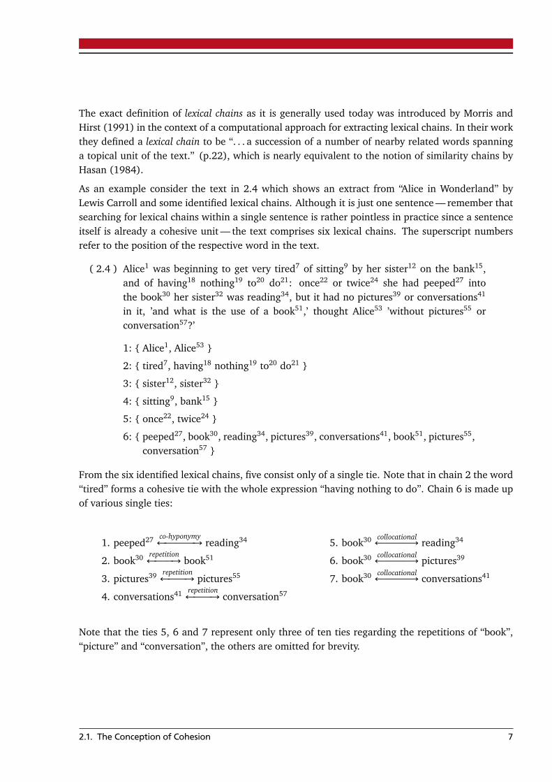
As an example consider the text in 2.4 which shows an extract from “Alice in Wonderland” byLewis Carroll and some identified lexical chains. Although it is just one sentence — remember thatsearching for lexical chains within a single sentence is rather pointless in practice since a sentenceitself is already a cohesive unit — the text comprises six lexical chains. The superscript numbersrefer to the position of the respective word in the text.
( 2.4 ) Alice1 was beginning to get very tired7 of sitting9 by her sister12 on the bank15,and of having18 nothing19 to20 do21: once22 or twice24 she had peeped27 intothe book30 her sister32 was reading34, but it had no pictures39 or conversations41
in it, ’and what is the use of a book51,’ thought Alice53 ’without pictures55 orconversation57?’
1: { Alice1, Alice53 }
2: { tired7, having18 nothing19 to20 do21 }
3: { sister12, sister32 }
4: { sitting9, bank15 }
5: { once22, twice24 }
6: { peeped27, book30, reading34, pictures39, conversations41, book51, pictures55,conversation57 }
From the six identified lexical chains, five consist only of a single tie. Note that in chain 2 the word“tired” forms a cohesive tie with the whole expression “having nothing to do”. Chain 6 is made upof various single ties:
1. peeped27 co-hyponymy←−−−−−→ reading34 5. book30 collocational←−−−−→ reading34
2. book30 repetition←−−−→ book51 6. book30 collocational←−−−−→ pictures39
3. pictures39 repetition←−−−→ pictures55 7. book30 collocational←−−−−→ conversations41
4. conversations41 repetition←−−−→ conversation57
Note that the ties 5, 6 and 7 represent only three of ten ties regarding the repetitions of “book”,“picture” and “conversation”, the others are omitted for brevity.
2.1. The Conception of Cohesion 7
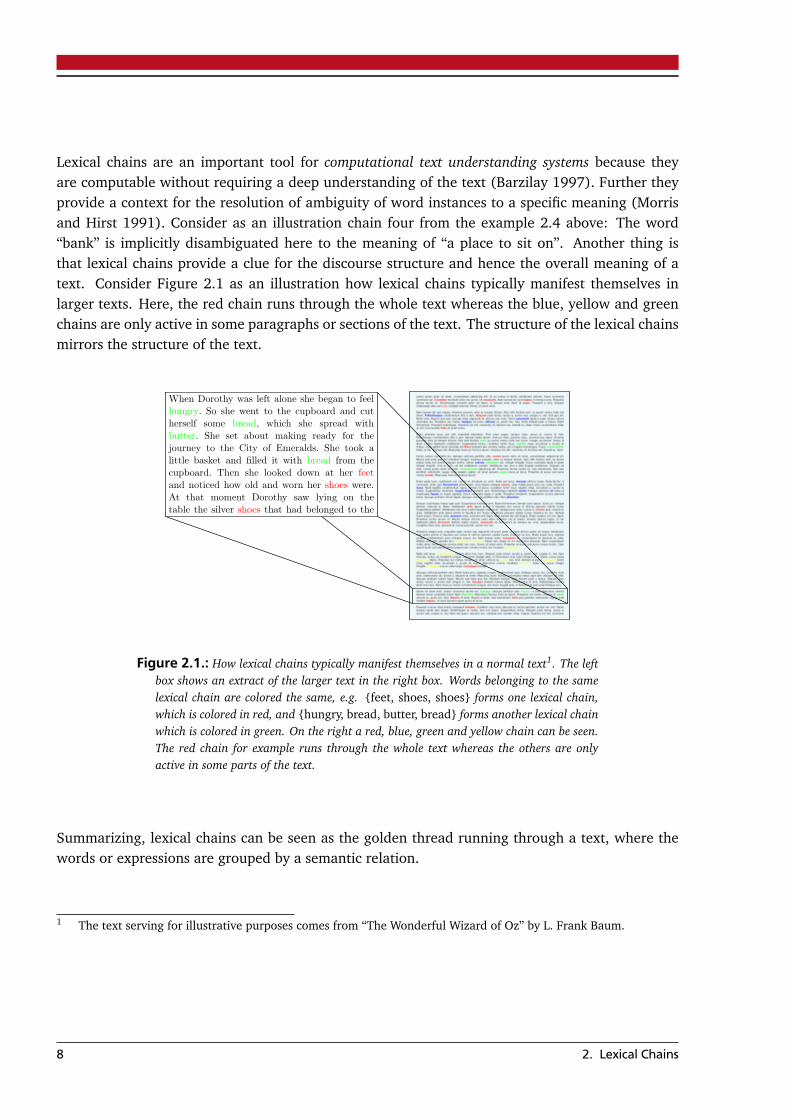
Lexical chains are an important tool for computational text understanding systems because theyare computable without requiring a deep understanding of the text (Barzilay 1997). Further theyprovide a context for the resolution of ambiguity of word instances to a specific meaning (Morrisand Hirst 1991). Consider as an illustration chain four from the example 2.4 above: The word“bank” is implicitly disambiguated here to the meaning of “a place to sit on”. Another thing isthat lexical chains provide a clue for the discourse structure and hence the overall meaning of atext. Consider Figure 2.1 as an illustration how lexical chains typically manifest themselves inlarger texts. Here, the red chain runs through the whole text whereas the blue, yellow and greenchains are only active in some paragraphs or sections of the text. The structure of the lexical chainsmirrors the structure of the text.
When Dorothy was left alone she began to feel hungry. So she went to the cupboard and cut herself some bread, which she spread with butter. She set about making ready for the journey to the City of Emeralds. She took a little basket and filled it with bread from the cupboard. Then she looked down at her feetand noticed how old and worn her shoes were. At that moment Dorothy saw lying on the table the silver shoes that had belonged to the
Figure 2.1.: How lexical chains typically manifest themselves in a normal text1. The leftbox shows an extract of the larger text in the right box. Words belonging to the samelexical chain are colored the same, e.g. {feet, shoes, shoes} forms one lexical chain,which is colored in red, and {hungry, bread, butter, bread} forms another lexical chainwhich is colored in green. On the right a red, blue, green and yellow chain can be seen.The red chain for example runs through the whole text whereas the others are onlyactive in some parts of the text.
Summarizing, lexical chains can be seen as the golden thread running through a text, where thewords or expressions are grouped by a semantic relation.
1 The text serving for illustrative purposes comes from “The Wonderful Wizard of Oz” by L. Frank Baum.
8 2. Lexical Chains
2.2 Lexical Chain Extraction Algorithms
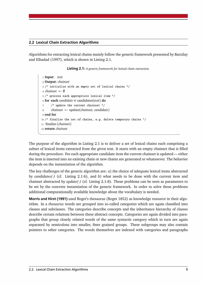
Algorithms for extracting lexical chains mainly follow the generic framework presented by Barzilayand Elhadad (1997), which is shown in Listing 2.1.
Listing 2.1: A generic framework for lexical chain extraction.
1 Input: text2 Output: chainset3 /* initialize with an empty set of lexical chains */
4 chainset ← ;5 /* process each appropriate lexical item */
6 for each candidate ∈ candidates(text) do7 /* update the current chainset */
8 chainset ← update(chainset, candidate)9 end for
10 /* finalize the set of chains, e.g. delete temporary chains */
11 finalize (chainset)12 return chainset�
The purpose of the algorithm in Listing 2.1 is to deliver a set of lexical chains each comprising asubset of lexical items extracted from the given text. It starts with an empty chainset that is filledduring the procedure. For each appropriate candidate item the current chainset is updated — eitherthe item is inserted into an existing chain or new chains are generated or whatsoever. The behaviordepends on the instantiation of the algorithm.
The key challenges of the generic algorithm are: a) the choice of adequate lexical items abstractedby candidates(·) (cf. Listing 2.1:6), and b) what needs to be done with the current item andchainset abstracted by update(·) (cf. Listing 2.1:8). These problems can be seen as parameters tobe set by the concrete instantiation of the generic framework. In order to solve these problemsadditional computationally available knowledge about the vocabulary is needed.
Morris and Hirst (1991) used Roget’s thesaurus (Roget 1852) as knowledge resource in their algo-rithm. In a thesaurus words are grouped into so-called categories which are again classified intoclasses and subclasses. The categories describe concepts and the inheritance hierarchy of classesdescribe certain relations between these abstract concepts. Categories are again divided into para-graphs that group closely related words of the same syntactic category which in turn are againseparated by semicolons into smaller, finer grained groups. These subgroups may also containpointers to other categories. The words themselves are indexed with categories and paragraphs
2.2. Lexical Chain Extraction Algorithms 9
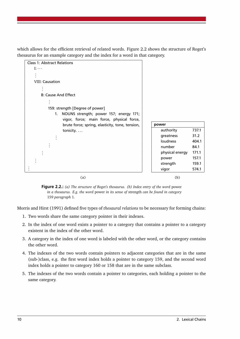
which allows for the efficient retrieval of related words. Figure 2.2 shows the structure of Roget’sthesaurus for an example category and the index for a word in that category.
Class 1: Abstract RelationsI: · · ·...VIII: Causation
...B: Cause And Effect
...159: strength [Degree of power]
1. NOUNS strength; power 157; energy 171;vigor, force; main force, physical force,brute force; spring, elasticity, tone, tension,tonicity. . . .
......
......
...
(a)
powerauthority 737.1greatness 31.2loudness 404.1number 84.1physical energy 171.1power 157.1strength 159.1vigor 574.1
(b)
Figure 2.2.: (a) The structure of Roget’s thesaurus. (b) Index entry of the word powerin a thesaurus. E.g. the word power in its sense of strength can be found in category159 paragraph 1.
Morris and Hirst (1991) defined five types of thesaural relations to be necessary for forming chains:
1. Two words share the same category pointer in their indexes.
2. In the index of one word exists a pointer to a category that contains a pointer to a categoryexistent in the index of the other word.
3. A category in the index of one word is labeled with the other word, or the category containsthe other word.
4. The indexes of the two words contain pointers to adjacent categories that are in the same(sub-)class, e.g. the first word index holds a pointer to category 159, and the second wordindex holds a pointer to category 160 or 158 that are in the same subclass.
5. The indexes of the two words contain a pointer to categories, each holding a pointer to thesame category.
10 2. Lexical Chains
Morris and Hirst allow at most one transitive link, which means if word a is related to word b andword b is related to word c, then a is also considered to be related to b. Additionally they limitedthe search scope to at most three sentences back, which means a word is unrelated if it is morethan three sentences back. Incidentally, Morris and Hirst defined the concept of chain returns insuch a case, but in this thesis, this will not be further regarded.
When processing a candidate item one of the above conditions must hold between any of theitems in existing chains and the candidate item, in which case, it is inserted into the chain whichcontains the related item; otherwise a new chain is created with the candidate item as singleelement. The candidate items are implicitly computed, by taking only those items into account,that are present in Roget’s thesaurus — ignoring pronouns, prepositions, verbal auxiliaries and highfrequency words such as good, do, etc. Although a machine readable thesaurus was not availableto Morris and Hirst in 1991, they showed that the algorithm delivers the desired structure definedby lexical cohesion.
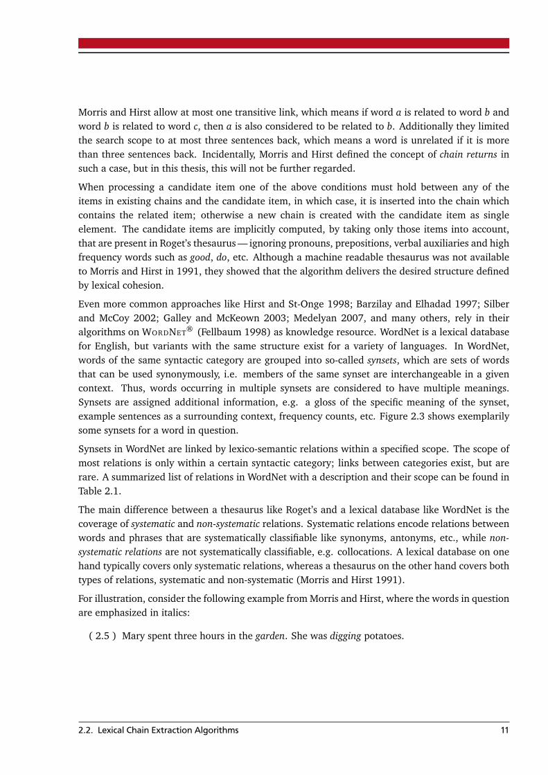
Even more common approaches like Hirst and St-Onge 1998; Barzilay and Elhadad 1997; Silberand McCoy 2002; Galley and McKeown 2003; Medelyan 2007, and many others, rely in theiralgorithms on WORDNET® (Fellbaum 1998) as knowledge resource. WordNet is a lexical databasefor English, but variants with the same structure exist for a variety of languages. In WordNet,words of the same syntactic category are grouped into so-called synsets, which are sets of wordsthat can be used synonymously, i.e. members of the same synset are interchangeable in a givencontext. Thus, words occurring in multiple synsets are considered to have multiple meanings.Synsets are assigned additional information, e.g. a gloss of the specific meaning of the synset,example sentences as a surrounding context, frequency counts, etc. Figure 2.3 shows exemplarilysome synsets for a word in question.
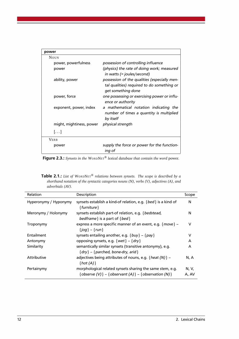
Synsets in WordNet are linked by lexico-semantic relations within a specified scope. The scope ofmost relations is only within a certain syntactic category; links between categories exist, but arerare. A summarized list of relations in WordNet with a description and their scope can be found inTable 2.1.
The main difference between a thesaurus like Roget’s and a lexical database like WordNet is thecoverage of systematic and non-systematic relations. Systematic relations encode relations betweenwords and phrases that are systematically classifiable like synonyms, antonyms, etc., while non-systematic relations are not systematically classifiable, e.g. collocations. A lexical database on onehand typically covers only systematic relations, whereas a thesaurus on the other hand covers bothtypes of relations, systematic and non-systematic (Morris and Hirst 1991).
For illustration, consider the following example from Morris and Hirst, where the words in questionare emphasized in italics:
( 2.5 ) Mary spent three hours in the garden. She was digging potatoes.
2.2. Lexical Chain Extraction Algorithms 11
powerNOUN
power, powerfulness possession of controlling influencepower (physics) the rate of doing work; measured
in watts (= joules/second)ability, power possession of the qualities (especially men-
tal qualities) required to do something orget something done
power, force one possessing or exercising power or influ-ence or authority
exponent, power, index a mathematical notation indicating thenumber of times a quantity is multipliedby itself
might, mightiness, power physical strength
[. . . ]
VERB
power supply the force or power for the function-ing of
Figure 2.3.: Synsets in the WORDNET® lexical database that contain the word power.
Table 2.1.: List of WORDNET® relations between synsets. The scope is described by ashorthand notation of the syntactic categories nouns (N), verbs (V), adjectives (A), andadverbials (AV).
Relation Description Scope
Hyperonymy / Hyponymy synsets establish a kind-of relation, e.g. {bed} is a kind of{furniture}
N
Meronymy / Holonymy synsets establish part-of relation, e.g. {bedstead,bedframe} is a part of {bed}
N
Troponymy express a more specific manner of an event, e.g. {move} –{jog} – {run}
V
Entailment synsets entailing another, e.g. {buy} – {pay} VAntonymy opposing synsets, e.g. {wet} – {dry} ASimilarity semantically similar synsets (transitive antonymy), e.g.
{dry} – {parched, bone-dry, arid}A
Attributive adjectives being attributes of nouns, e.g. {heat (N)} –{hot (A)}
N, A
Pertainymy morphological related synsets sharing the same stem, e.g.{observe (V)} – {observant (A)} – {observation (N)}
N, V,A, AV
12 2. Lexical Chains
In WordNet the words “garden” and “digging” are not related, even not by a path of any length.Roget’s on the other hand contains a category “agriculture” which includes both words.
Hirst and St-Onge (1998) were one of the first who approached the lexical chaining task utilizingWordNet instead of a thesaurus where they defined the necessary lexical relations that replacethe necessary thesaural relations originally defined by Morris and Hirst (1991). Hirst and St-Ongedefined three types of relations for tying up words or phrases:
extra strong: holding between a word and its literal repetition;
strong: holding between words when they (a) are in the same synset, (b) one of their synsets areconnected by antonymy or similarity, or (c) one word is a compound or phrase that containsthe other and one of their synsets are connected by any kind of relation;
medium strong: holding between words when one of their synsets are connected by a path be-tween two and five links of any kind of relation, where the path is restricted by the followingrules: (a) if a hypernymic relation is in the path, it must be the first step, and (b) at most onegeneralization followed by a specification is allowed. Additionally a medium strong relationis assigned a weight calculated from the kind of relations used in the path and the length ofthe path. Details can be found in (Hirst and St-Onge 1998).
Hirst and St-Onge addressed the candidates(·) problem in Listing 2.1 by processing everyword — ignoring pronouns, prepositions, verbal auxiliaries and high frequency words — and treat-ing each word as a noun, i.e. for every appropriate word the noun file of WordNet was checked forexisting synset entries, as the assumption is that most words of other grammatical categories thathave a nominal form are likely to be semantically close to that form. Their choice of the “nounsubnet” as entry point has some good reasons. First, it contains by far the most synsets and synsetrelations, and second, a part-of-speech tagger as a preprocessing step can be omitted.
While processing candidate items, Hirst and St-Onge keep a reference to the synsets in use in eachof the chains. Based on the type of relation (extra strong, strong, medium strong) synsets areremoved from further consideration. Unrelated candidate items — the first occurring candidateitem also counts as unrelated — are inserted into a new chain, and the item keeps a reference toeach of the synsets it occurs in. If a candidate item is related to two or more lexical items in distinctchains, the respective chains are merged. Next, if an extra strong relation is encountered, nothing isremoved at all, since the words can not be disambiguated; if a strong relation is encountered, onlythe pairs of strongly connected synsets are kept; and if a medium strong relation is encounteredonly the highest weighted synset is kept.
Barzilay and Elhadad (1997) noted that by processing the candidate items in the order of their oc-currence, lexical items may be disambiguated falsely. Barzilay and Elhadad illustrated the problemwith an example, recited in example 2.6.
2.2. Lexical Chain Extraction Algorithms 13
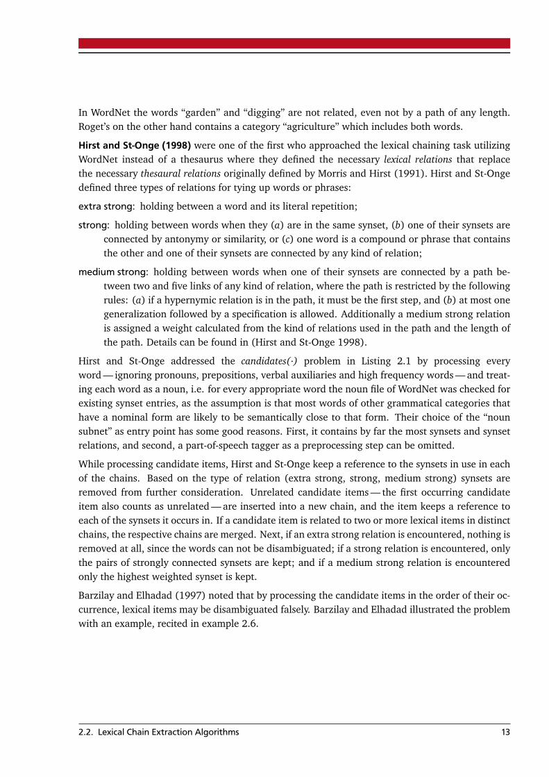
( 2.6 ) Mr. Kenny is the person that invented an anesthetic machine which uses micro-computers to control the rate at which an anesthetic is pumped into the blood.Such machines are nothing new. But his device uses two micro-computers toachieve much closer monitoring of the pump feeding the anesthetic into the pa-tient. [. . . ]
According to Hirst and St-Onge’s method, the underlined candidate words are processed in orderof their occurrence. First, the word “Mr” is inserted into the chainset as a new chain, which is im-plicitly disambiguated, just because it is in only one synset. Second, the word “person” is insertedinto the same chain because of a medium strong relation between “Mr” and “person”, which keepsonly a reference to the highest weighted synset named “a human being”. Third, the word “ma-chine” is processed. Because a strong relation holds between “person” and “machine” — in one ofits synsets, “machine” is interpreted as a “very efficient person”, which is in a hypernymic relationto “a human being” — it is inserted into the current {“Mr”, “person”} chain. This is obviously thewrong behavior; the word “machine” is disambiguated falsely at this step. This tough problem ofword sense disambiguation engages a lot of research in the field of computational linguistics.
Barzilay and Elhadad (1997) address this problem by keeping a list of interpretations of variouscomponents — a component is a set of relatable words, i.e. words that may but do not have toform a single chain, and an interpretation is the combination of words resulting in a specific setof chains — of the text, until in the end the strongest interpretation of each component is chosen.In order to discriminate the various interpretations qualitatively, Barzilay and Elhadad defined thestrength for an interpretation to be the sum of the weights of the chains it inheres. The weight of achain is the sum of the weights of existing relations in the respective chain. Barzilay and Elhadaddefined two terms to be related by a lexical relation with a weight of (a) 10 if they are identical,or in the same synset, (b) 8 if one of their synsets are in a path in the hypernym hierarchy (c) 7 ifone of their synsets are antonyms, (d) 4 if one of their synsets are meronyms, (e) 2 if one of theirsynsets are co-hyponyms with a maximum degree of 4. More details about the used weightingscheme can be found in Barzilay (1997, pp.32–33).
Barzilay and Elhadad’s update procedure is best described with the example they provided. Recon-sider therefore example 2.6 from above. In the second step, the word “person” is related to “Mr”,so “person” is added to the component containing “Mr” and the interpretations are updated to:
interpretations before interpretations after
{Mr}{Mr, person}{Mr}, {person}
In the third step “machine” is related to “person” and “Mr”, and so it is inserted into the componentthat contains “person” and “Mr”. The interpretations are then updated to:
14 2. Lexical Chains
interpretations before interpretations after
{Mr, person}{Mr, person, machine}{Mr, person}, {machine}
{Mr}, {person}{Mr}, {person}, {machine}{Mr, machine}, {person}{Mr}, {person, machine}
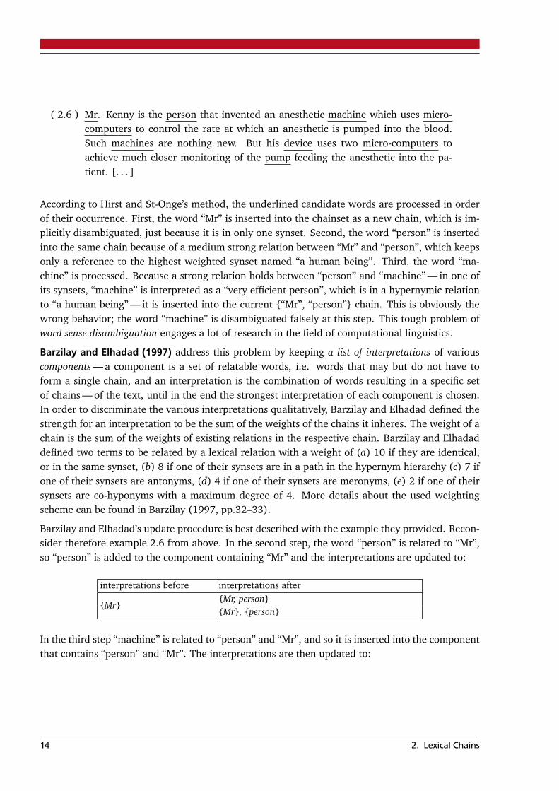
Next, “micro-computers” is inserted into the component containing “machine”, because of a re-lation between those two. Because of an exponential growth only the update of the first twointerpretations resulting from the last step are shown:
interpretations before interpretations after
{Mr, person, machine}{Mr, person, machine, micro-computers}{Mr, person, machine}, {micro-computers}
{Mr, person}, {machine}{Mr, person}, {machine, micro-computers}{Mr, person}, {machine}, {micro-computers}
[. . . ]
Proceeding until the last word was inserted results in a number of interpretations each havinga certain weight. According to Barzilay and Elhadad the strongest interpretation and thus theresulting chainset for the running example is {{“Mr”, “person”}, {“machine”, “micro-computers”,“machines”, “device”, “micro-computers”, “pump”}}, which clearly follows the intuition. In orderto limit the computational complexity, the search scope is limited to the segment, where the can-didate item is located. Segments are computed beforehand using the segmentation algorithm byHearst (1994).
Barzilay and Elhadad (1997) consider nouns as possible candidate items — excluding modifiersof noun compounds. Nouns are identified by a part-of-speech tagger and compound nouns aredetected heuristically. Unfortunately the algorithm has an exponential complexity in time andspace — exclusive of the three preprocessing steps — which makes it impractical for the use withlarger documents.
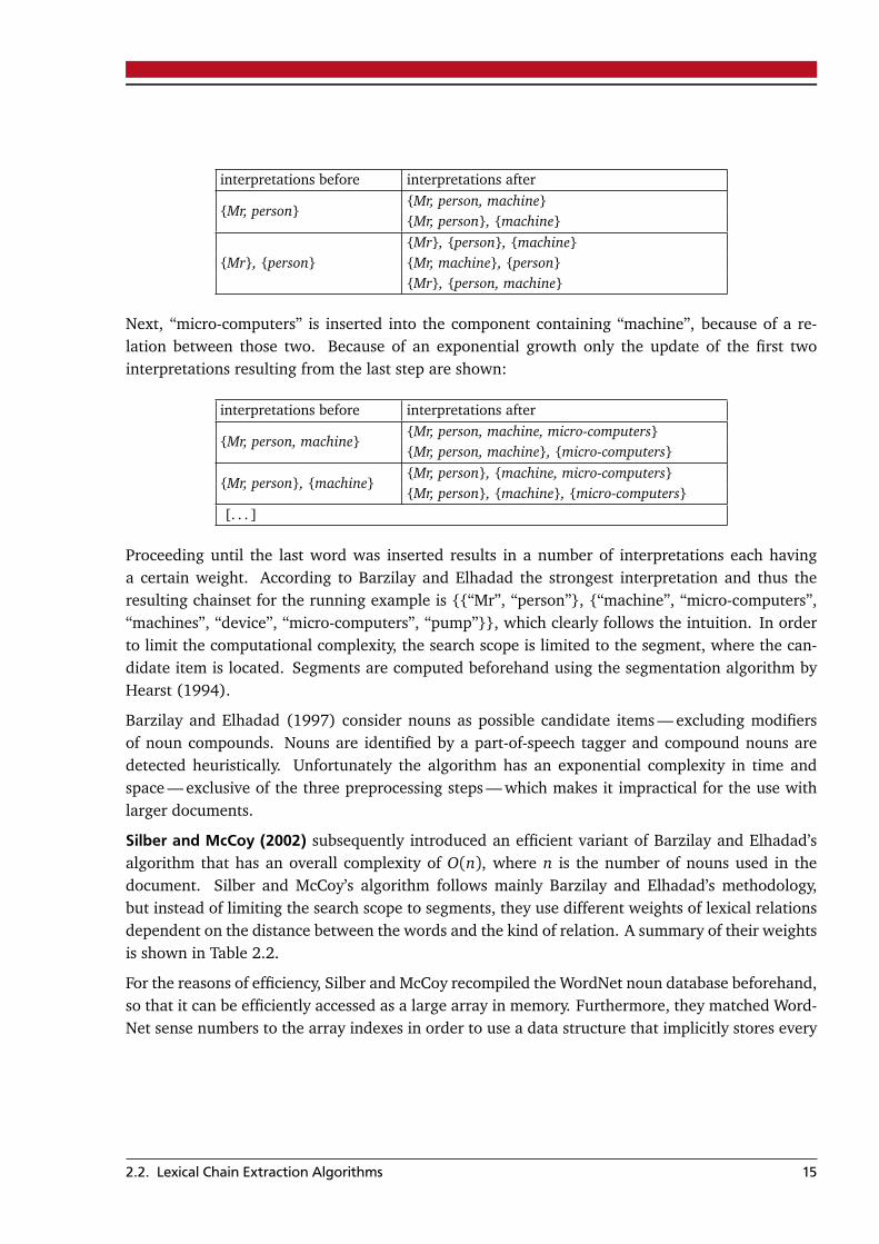
Silber and McCoy (2002) subsequently introduced an efficient variant of Barzilay and Elhadad’salgorithm that has an overall complexity of O(n), where n is the number of nouns used in thedocument. Silber and McCoy’s algorithm follows mainly Barzilay and Elhadad’s methodology,but instead of limiting the search scope to segments, they use different weights of lexical relationsdependent on the distance between the words and the kind of relation. A summary of their weightsis shown in Table 2.2.
For the reasons of efficiency, Silber and McCoy recompiled the WordNet noun database beforehand,so that it can be efficiently accessed as a large array in memory. Furthermore, they matched Word-Net sense numbers to the array indexes in order to use a data structure that implicitly stores every
2.2. Lexical Chain Extraction Algorithms 15
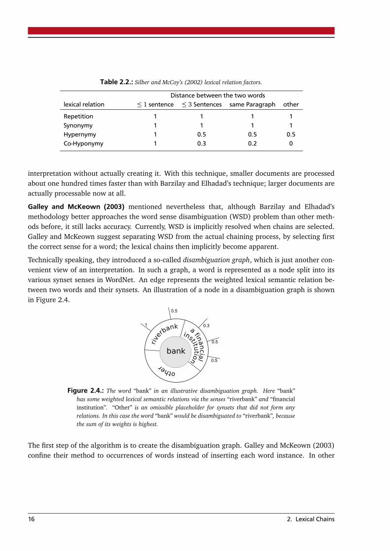
Table 2.2.: Silber and McCoy’s (2002) lexical relation factors.
Distance between the two wordslexical relation ≤ 1 sentence ≤ 3 Sentences same Paragraph other
Repetition 1 1 1 1Synonymy 1 1 1 1Hypernymy 1 0.5 0.5 0.5Co-Hyponymy 1 0.3 0.2 0
interpretation without actually creating it. With this technique, smaller documents are processedabout one hundred times faster than with Barzilay and Elhadad’s technique; larger documents areactually processable now at all.
Galley and McKeown (2003) mentioned nevertheless that, although Barzilay and Elhadad’smethodology better approaches the word sense disambiguation (WSD) problem than other meth-ods before, it still lacks accuracy. Currently, WSD is implicitly resolved when chains are selected.Galley and McKeown suggest separating WSD from the actual chaining process, by selecting firstthe correct sense for a word; the lexical chains then implicitly become apparent.
Technically speaking, they introduced a so-called disambiguation graph, which is just another con-venient view of an interpretation. In such a graph, a word is represented as a node split into itsvarious synset senses in WordNet. An edge represents the weighted lexical semantic relation be-tween two words and their synsets. An illustration of a node in a disambiguation graph is shownin Figure 2.4.
bank
a
financia
l
rive
rbank
institution
other
0.5
1 0.3
0.5
0.5
Figure 2.4.: The word “bank” in an illustrative disambiguation graph. Here “bank”has some weighted lexical semantic relations via the senses “riverbank” and “financialinstitution”. “Other” is an omissible placeholder for synsets that did not form anyrelations. In this case the word “bank” would be disambiguated to “riverbank”, becausethe sum of its weights is highest.
The first step of the algorithm is to create the disambiguation graph. Galley and McKeown (2003)confine their method to occurrences of words instead of inserting each word instance. In other
16 2. Lexical Chains
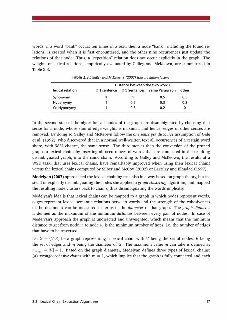
words, if a word “bank” occurs ten times in a text, then a node “bank”, including the found re-lations, is created when it is first encountered, and the other nine occurrences just update therelations of that node. Thus, a “repetition” relation does not occur explicitly in the graph. Theweights of lexical relations, empirically evaluated by Galley and McKeown, are summarized inTable 2.3.
Table 2.3.: Galley and McKeown’s (2002) lexical relation factors.
Distance between the two wordslexical relation ≤ 1 sentence ≤ 3 Sentences same Paragraph other
Synonymy 1 1 0.5 0.5Hypernymy 1 0.5 0.3 0.3Co-Hyponymy 1 0.3 0.2 0
In the second step of the algorithm all nodes of the graph are disambiguated by choosing thatsense for a node, whose sum of edge weights is maximal, and hence, edges of other senses areremoved. By doing so Galley and McKeown follow the one sense per discourse assumption of Galeet al. (1992), who discovered that in a normal well-written text all occurrences of a certain wordshare, with 98% chance, the same sense. The third step is then the conversion of the prunedgraph to lexical chains by inserting all occurrences of words that are connected in the resultingdisambiguated graph, into the same chain. According to Galley and McKeown, the results of aWSD task, that uses lexical chains, have remarkably improved when using their lexical chainsversus the lexical chains computed by Silber and McCoy (2002) or Barzilay and Elhadad (1997).
Medelyan (2007) approached the lexical chaining task also in a way based on graph theory, but in-stead of explicitly disambiguating the nodes she applied a graph clustering algorithm, and mappedthe resulting node clusters back to chains, thus disambiguating the words implicitly.
Medelyan’s idea is that lexical chains can be mapped to a graph in which nodes represent words,edges represent lexical semantic relations between words and the strength of the cohesivenessof the document can be measured in terms of the diameter of that graph. The graph diameteris defined as the maximum of the minimum distances between every pair of nodes. In case ofMedelyan’s approach the graph is undirected and unweighted, which means that the minimumdistance to get from node v i to node v j is the minimum number of hops, i.e. the number of edgesthat have to be traversed.
Let G = (V, E) be a graph representing a lexical chain with V being the set of nodes, E beingthe set of edges and m being the diameter of G. The maximum value m can take is defined asmmax = |V | − 1. Based on the graph diameter, Medelyan defines three types of lexical chains:(a) strongly cohesive chains with m = 1, which implies that the graph is fully connected and each
2.2. Lexical Chain Extraction Algorithms 17
word is directly related to each other, (b) moderately cohesive chains: with 1 < m < mmax , and(c) weakly cohesive chains: with m= mmax .
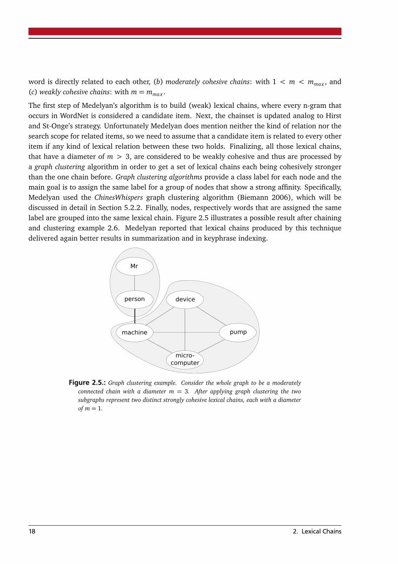
The first step of Medelyan’s algorithm is to build (weak) lexical chains, where every n-gram thatoccurs in WordNet is considered a candidate item. Next, the chainset is updated analog to Hirstand St-Onge’s strategy. Unfortunately Medelyan does mention neither the kind of relation nor thesearch scope for related items, so we need to assume that a candidate item is related to every otheritem if any kind of lexical relation between these two holds. Finalizing, all those lexical chains,that have a diameter of m > 3, are considered to be weakly cohesive and thus are processed bya graph clustering algorithm in order to get a set of lexical chains each being cohesively strongerthan the one chain before. Graph clustering algorithms provide a class label for each node and themain goal is to assign the same label for a group of nodes that show a strong affinity. Specifically,Medelyan used the ChinesWhispers graph clustering algorithm (Biemann 2006), which will bediscussed in detail in Section 5.2.2. Finally, nodes, respectively words that are assigned the samelabel are grouped into the same lexical chain. Figure 2.5 illustrates a possible result after chainingand clustering example 2.6. Medelyan reported that lexical chains produced by this techniquedelivered again better results in summarization and in keyphrase indexing.
Mr
person
machine
device
micro-computer
pump
Figure 2.5.: Graph clustering example. Consider the whole graph to be a moderatelyconnected chain with a diameter m = 3. After applying graph clustering the twosubgraphs represent two distinct strongly cohesive lexical chains, each with a diameterof m= 1.
18 2. Lexical Chains
2.3 Desiderata for Lexical Chain Annotation
Other algorithms beside the ones explained before exist, each extracting lexical chains in a slightlydifferent way and with another goal in mind. E.g. Okumura and Honda (1994) performed wordsense disambiguation utilizing lexical chains, Stairmand (1996) used lexical chains in informationretrieval, Green (1996) used lexical chains for creating hypertext links, Al-Halimi and Kazman(1998) indexed video conferences in a database, Moldovan and Novischi (2002) approached thetask of question answering, Jarmasz (2003) introduced the ELKB2 and used it for lexical chainextraction, Stokes et al. (2004) segmented news story with the help of lexical chains, Teich andFankhauser (2005) analyzed lexical chains with respect to different registers, Reeve et al. (2006)used lexical chains for summarization in the biomedical domain, Yang and Powers (2006) utilizedthe EAT3 for extracting lexical chains and performed word sense disambiguation, Ercan and Ci-cekli (2007) extracted keywords using lexical chains, Marathe and Hirst (2010) utilized DMCDs4
for extracting lexical chains and evaluated them by text segmentation, etc. The list seems endless,and in fact, even when they are not extracted as an intermediate tool, lexical chains are implic-itly assumed in nearly every natural language processing task that deals with some kind of textunderstanding simply because it is assumed that the text is cohesive.
The main problem when developing a new lexical chaining algorithm is the comparison to previoussystems. Most of the techniques mentioned before claim to produce better lexical chains than themethods before. This is substantiated by the evaluation of a certain task like summarization, wordsense disambiguation, or keyphrase extraction using their computed lexical chains and lexicalchains produced by other systems. Since lexical chains are mostly used as an intermediate stepand the parameter details are very fine grained, little changes may have a deep impact in theoutcome of the certain task. Also, reproducibility is mostly impossible due to the brevity in givendetails. Thus the result of each evaluation is, in part, always subjectively influenced. What isgenerally needed are objective criteria for directly comparing lexical chains.
Strictly speaking a generally accepted corpus is needed, manually annotated with lexical chaininformation, available for everybody, so that every new algorithm may be evaluated using thiscorpus, presenting its result using a generally accepted evaluation measure. Both claims will beaddressed in the next chapters, starting with the question for a good lexical chain comparisonmeasure.
2 http://rogets.site.uottawa.ca – The Electronic Lexical Knowledge Base (ELKB) is an electronic version of Roget’sthesaurus.
3 http://www.eat.rl.ac.uk – The Edinburgh Associative Thesaurus (EAT) contains spontaneous responses for a givenword.
4 Distributional measures of Concept Distance (DMCDs) combine distributional co-occurrence information withsemantic information from a lexicographic resource (Marathe and Hirst 2010).
2.3. Desiderata for Lexical Chain Annotation 19

20 2. Lexical Chains
3 Comparing Lexical ChainsOnce different sets of lexical chains of the same text are available — coming either from manualannotation or as a result of automatic chaining algorithms — they need to be compared in orderto qualitatively say how similar or how different they are; i.e. the degree of agreement must bemeasured. Unfortunately, the comparison of lexical chains is a non-trivial task. A first methodol-ogy was performed by Morris and Hirst (2004) in a user study where annotators were asked to(a) identify “word groups” (i.e. lexical chains) in various texts, and (b) mark words that they per-ceived to have a direct relation. The resulting data was then analyzed as follows: First, Morris andHirst measured the pairwise agreement between annotators on the lexical items they used in termsof accuracy and then averaged it with the accuracy of all possible pairs of annotators. Hereby, theycollected all items annotated by a pair of annotators and used the complete set of items as thereference set for computing the relative amount of items on which the annotators agreed. Theresults of all pairs of annotators are then averaged:
Item-Accuracy=1
n(n− 1)/2
∑
i, j ∈ Annotators
Item-Accuracyi j where n= |Annotators| (3.1)
Item-Accuracyi j =# i tems annotatori AN D annotator j identi f ied
# i tems annotatori OR annotator j identi f ied(3.2)
In the next step, they measured the agreement on prevalent word pairs that were often markedas directly related within the word groups. Here, Morris and Hirst matched the word groups ofindividual annotators to global ones (i.e. word groups annotated by the majority of annotators),and used only those word pairs that were marked by at least 50% of the annotators. On that basis,they computed the average accuracy for each word pair as:
Word-Pair-Accuracy=1
n
∑
i ∈ Annotators
Word-Pair-Accuracyi (3.3)
Word-Pair-Accuracyi =# word pairs marked b y annotatori
# word pairs marked any annotator(3.4)
Although the intention of Morris and Hirst for using these measures is to qualitatively measurethe subjectivity of lexical chaining, the methodology they introduced can also be used to compare
21
lexical chains produced by different annotators. However, the manual selection steps are notacceptable in an automatic evaluation framework.
Another approach for measuring the similarity of lexical chains was performed by Hollingsworthand Teufel (2005). They treated each individual lexical chain as a set of words and all chains ofa particular document are treated as a set of lexical chains, a so-called chain set. They comparedfour measures in terms of their suitability for measuring similarity between chain sets produced bydifferent annotators:
1. cosine similarity metric
2. Kullback Leibler distance
3. strict term overlap
4. partial term overlap (analogous to strict term overlap, but splitting compound terms into theirindividual parts before measuring term overlap).
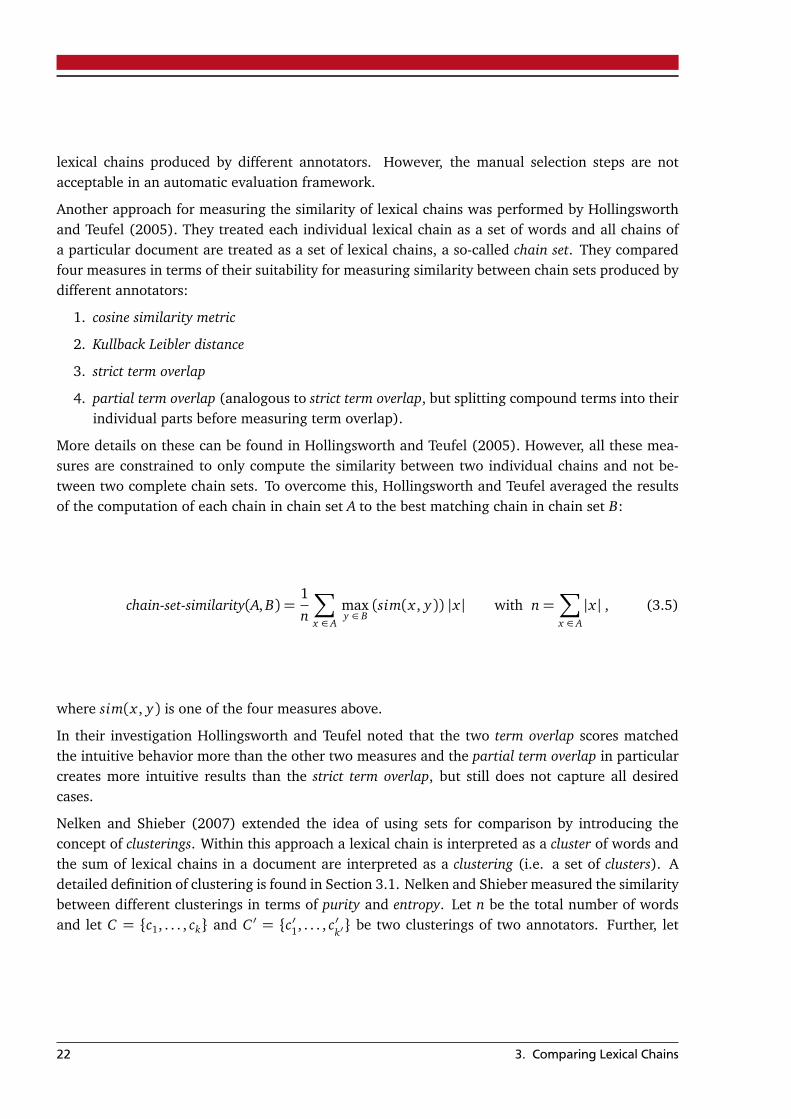
More details on these can be found in Hollingsworth and Teufel (2005). However, all these mea-sures are constrained to only compute the similarity between two individual chains and not be-tween two complete chain sets. To overcome this, Hollingsworth and Teufel averaged the resultsof the computation of each chain in chain set A to the best matching chain in chain set B:
chain-set-similarity(A, B) =1
n
∑
x ∈ A
maxy ∈ B
(sim(x , y)) |x | with n=∑
x ∈ A
|x | , (3.5)
where sim(x , y) is one of the four measures above.
In their investigation Hollingsworth and Teufel noted that the two term overlap scores matchedthe intuitive behavior more than the other two measures and the partial term overlap in particularcreates more intuitive results than the strict term overlap, but still does not capture all desiredcases.
Nelken and Shieber (2007) extended the idea of using sets for comparison by introducing theconcept of clusterings. Within this approach a lexical chain is interpreted as a cluster of words andthe sum of lexical chains in a document are interpreted as a clustering (i.e. a set of clusters). Adetailed definition of clustering is found in Section 3.1. Nelken and Shieber measured the similaritybetween different clusterings in terms of purity and entropy. Let n be the total number of wordsand let C = {c1, . . . , ck} and C ′ = {c′1, . . . , c′
k′} be two clusterings of two annotators. Further, let
22 3. Comparing Lexical Chains
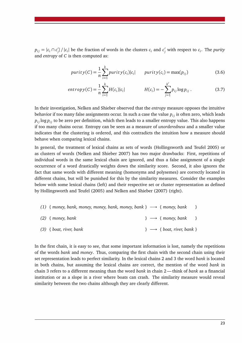
pi j = |ci ∩ c′j|/ |ci| be the fraction of words in the clusters ci and c′j with respect to ci. The purityand entropy of C is then computed as:
puri t y(C) =1
n
k∑
i=1
puri t y(ci)|ci| puri t y(ci) =max(pi j) (3.6)
ent rop y(C) =1
n
k∑
i=1
H(ci)|ci| H(ci) =−k′∑
j=1
pi j log pi j . (3.7)
In their investigation, Nelken and Shieber observed that the entropy measure opposes the intuitivebehavior if too many false assignments occur. In such a case the value pi j is often zero, which leadspi j log pi j to be zero per definition, which then leads to a smaller entropy value. This also happensif too many chains occur. Entropy can be seen as a measure of unorderedness and a smaller valueindicates that the clustering is ordered, and this contradicts the intuition how a measure shouldbehave when comparing lexical chains.
In general, the treatment of lexical chains as sets of words (Hollingsworth and Teufel 2005) oras clusters of words (Nelken and Shieber 2007) has two major drawbacks: First, repetitions ofindividual words in the same lexical chain are ignored, and thus a false assignment of a singleoccurrence of a word drastically weights down the similarity score. Second, it also ignores thefact that same words with different meaning (homonyms and polysemes) are correctly located indifferent chains, but will be punished for this by the similarity measures. Consider the examplesbelow with some lexical chains (left) and their respective set or cluster representation as definedby Hollingsworth and Teufel (2005) and Nelken and Shieber (2007) (right).
(1) { money, bank, money, money, bank, money, bank } −→ { money, bank }
(2) { money, bank } −→ { money, bank }
(3) { boat, river, bank } −→ { boat, river, bank }
In the first chain, it is easy to see, that some important information is lost, namely the repetitionsof the words bank and money. Thus, comparing the first chain with the second chain using theirset representation leads to perfect similarity. In the lexical chains 2 and 3 the word bank is locatedin both chains, but assuming the lexical chains are correct, the mention of the word bank inchain 3 refers to a different meaning than the word bank in chain 2 — think of bank as a financialinstitution or as a slope in a river where boats can crash. The similarity measure would revealsimilarity between the two chains although they are clearly different.
23
This thesis derives a methodology which is also based on the idea of interpreting lexical chainsas clusters, but in contrast to the suggestion of Hollingsworth and Teufel (2005) or Nelken andShieber (2007), the elements in a cluster will be some unique identifier of the respective word inthe text. This way, repetitions of certain words will not be truncated. Additionally an extensiveinvestigation will be presented, which illustrates the suitability of various standard measures usedin clustering comparison, for the task of comparing lexical chains.
3.1 Clustering Defintion
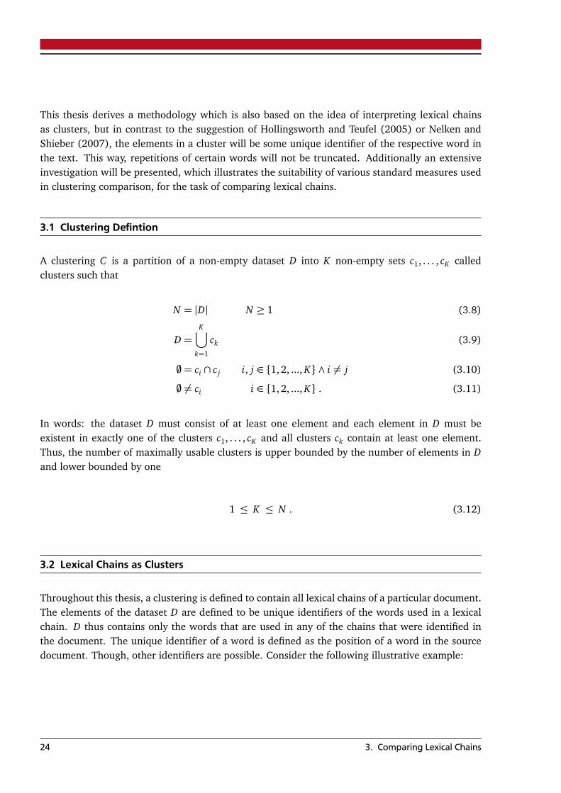
A clustering C is a partition of a non-empty dataset D into K non-empty sets c1, . . . , cK calledclusters such that
N = |D| N ≥ 1 (3.8)
D =K⋃
k=1
ck (3.9)
;= ci ∩ c j i, j ∈ {1,2, ..., K} ∧ i 6= j (3.10)
; 6= ci i ∈ {1,2, ..., K} . (3.11)
In words: the dataset D must consist of at least one element and each element in D must beexistent in exactly one of the clusters c1, . . . , cK and all clusters ck contain at least one element.Thus, the number of maximally usable clusters is upper bounded by the number of elements in Dand lower bounded by one
1 ≤ K ≤ N . (3.12)
3.2 Lexical Chains as Clusters
Throughout this thesis, a clustering is defined to contain all lexical chains of a particular document.The elements of the dataset D are defined to be unique identifiers of the words used in a lexicalchain. D thus contains only the words that are used in any of the chains that were identified inthe document. The unique identifier of a word is defined as the position of a word in the sourcedocument. Though, other identifiers are possible. Consider the following illustrative example:
24 3. Comparing Lexical Chains
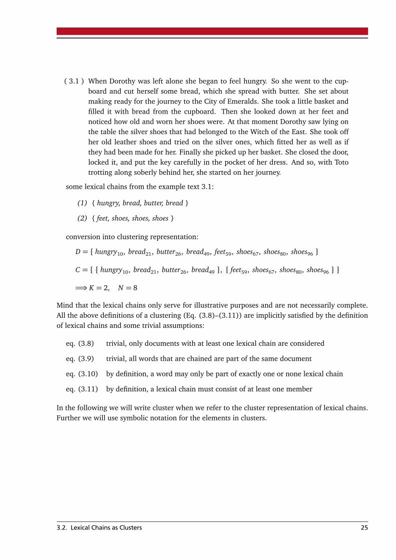
( 3.1 ) When Dorothy was left alone she began to feel hungry. So she went to the cup-board and cut herself some bread, which she spread with butter. She set aboutmaking ready for the journey to the City of Emeralds. She took a little basket andfilled it with bread from the cupboard. Then she looked down at her feet andnoticed how old and worn her shoes were. At that moment Dorothy saw lying onthe table the silver shoes that had belonged to the Witch of the East. She took offher old leather shoes and tried on the silver ones, which fitted her as well as ifthey had been made for her. Finally she picked up her basket. She closed the door,locked it, and put the key carefully in the pocket of her dress. And so, with Tototrotting along soberly behind her, she started on her journey.
some lexical chains from the example text 3.1:
(1) { hungry, bread, butter, bread }
(2) { feet, shoes, shoes, shoes }
conversion into clustering representation:
D = { hungry10, bread21, butter26, bread49, feet59, shoes67, shoes80, shoes96 }
C = { { hungry10, bread21, butter26, bread49 }, { feet59, shoes67, shoes80, shoes96 } }
=⇒ K = 2, N = 8
Mind that the lexical chains only serve for illustrative purposes and are not necessarily complete.All the above definitions of a clustering (Eq. (3.8)–(3.11)) are implicitly satisfied by the definitionof lexical chains and some trivial assumptions:
eq. (3.8) trivial, only documents with at least one lexical chain are considered
eq. (3.9) trivial, all words that are chained are part of the same document
eq. (3.10) by definition, a word may only be part of exactly one or none lexical chain
eq. (3.11) by definition, a lexical chain must consist of at least one member
In the following we will write cluster when we refer to the cluster representation of lexical chains.Further we will use symbolic notation for the elements in clusters.
3.2. Lexical Chains as Clusters 25
3.3 Comparing Clusterings
Suppose a clustering C was built of lexical chains in a particular document and suppose further asecond clustering C ′ was built of another set of lexical chains from the same document. The taskis now to measure how close C and C ′ are.
3.3.1 Cluster Conformation
Though created from the same document, the choice of lexical items during the chaining process isaccompanied by subjectivity and thus the datasets D and D′ spanned by C and C ′ respectively maybe different. In order to compare a clustering C to a clustering C ′ it is a convenient preprocessingstep to produce conformity within the underlying datasets such that D = D′. Since we do not wantto ignore any decisions made in any of the clusterings, we transform C and C ′ to reflect the unionof the datasets of each other (D ∪ D′).
Two options are now possible conformations: (a) inserting each missing item as a single cluster, or(b) inserting each missing item into the same single cluster. Because each lexical item is assigned acertain meaning, mixing meanings, as would be the case in option b, is counterintuitive, and thusoption a is chosen, and missing items are inserted as single clusters as formalized below:
C := C ∪ {d ′1} ∪ · · · ∪ {d′n} d ′1, . . . , d ′n ∈ D′ \ D
C ′ := C ′ ∪ {d1} ∪ · · · ∪ {dn} d1, . . . , dn ∈ D \ D′ .(3.13)
As an illustrative example consider C = {{a, b}, {c}} and C ′ = {{a, d}, {e, f }}. After applying theequations in (3.13) we have C = {{a, b}, {c}, {d}, {e}, { f }} and C ′ = {{a, d}, {e, f }, {b}, {c}}. Notethat conformity is a prerequisite of the measures below, it is thus assumed that two clusterings Cand C ′, that are to be compared, are conformed by the above technique before measuring similarity.We then only speak of a dataset D instead of D and D′ because D = D′, and C and C ′ are simplytwo different clusterings of the same dataset.
3.3.2 Desirable Properties
As stated by Meila (2005) and Amigó et al. (2009) a best clustering comparison measure for thegeneral case does not exist. Meila (2005) proved that it is simply impossible for any clusteringcomparison measure to satisfy all comparison criteria she presented. As it is, she examined variousmeasures and proposed one — the variation of information (Meila 2003, 2007) — that fulfills allher criteria but one. Amigó et al. (2009) did a similar investigation and compiled some formalconstraints that any clustering measure should satisfy. In their work, they pointed out that the
26 3. Comparing Lexical Chains
only clustering measure satisfying all of their four constraints is the B3 measure by Bagga andBaldwin (1998). However, Meila as well as Amigó et al. stressed that the clustering measure to usehighly depends on the task at hand.
In the following some basic properties are listed that should be reflected by a good measure forcomparing lexical chains:
1. The measure should be a value between zero and one:
sim(C , C ′) ∈ [0,1] ⊂ R .
2. The measure should be maximal when C = C ′ and not maximal when C 6= C ′:
sim(C , C ′) =
¨
1 if C = C ′ ,< 1 otherwise
.
Note that a distance measure d(C , C ′) with 0 ≤ d(C , C ′) ≤ 1 and d(C , C ′) = 0 if C = C ′
can also be interpreted as a dissimilarity measure and thus converted to a similarity measure:
sim(C , C ′) = 1− d(C , C ′) .
3. The measure should be minimal when D and D′ have no items in common before conforma-tion (cf. Sec. 3.3.1):
sim(C , C ′) = 0 if D ∩ D′ = ; .
After applying the equations in (3.13) D and D′ share the same elements per definition.
4. The measure should be symmetric:
sim(C , C ′) = sim(C ′, C) .
This is due to the fact that the measure will be used for inter-annotator agreement, wherethere is no way to distinguish which clustering is the gold clustering. Note that symmetry canalways be forced by sims ymmet ric(C , C ′) = 1/2 simas ymmet ric(C , C ′) + 1/2 simas ymmet ric(C ′, C).
5. Simple basic transformations should be reflected by the same difference in the value:
|sim(C , t rans1(C))− sim(C , t rans2(C))|= 0 ,
where t rans1(·) and t rans2(·) are different basic operations, for example splitting a clusterinto two or merging two clusters into one, etc. Figure 3.1b to 3.1j show some clusteringswhere just some basic operations are needed to get the gold clustering in 3.1a.
3.3. Comparing Clusterings 27
The list of properties is not necessarily complete, other properties, e.g. the independence of datasetsize or the number of clusters, are also valuable, but the above are perceived as the most impor-tant ones for the task of comparing two separate sets of lexical chains extracted from the samedocument.
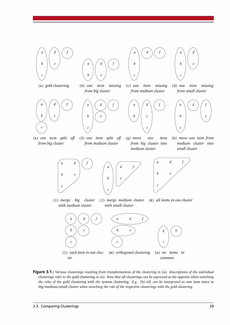
In the next sections some selected measures will be analyzed for their suitability of the current task.For this, the measures will be i.a. used for comparing artificially created clusterings as illustratedin Figure 3.1 where the desired clustering is shown in 3.1a and the similarity is calculated againstthe clusterings in 3.1b–3.1n.
28 3. Comparing Lexical Chains
a d f
b e
c
(a) gold clustering
a d f
b e
(b) one item missingfrom big cluster
a d f
b
c
(c) one item missingfrom medium cluster
a d
b e
c
(d) one item missingfrom small cluster
a d f
b e
c
(e) one item split offfrom big cluster
a d f
b e
c
(f) one item split offfrom medium cluster
a d f
b e
c
(g) move one itemfrom big cluster intomedium cluster
a d f
b e
c
(h) move one item frommedium cluster intosmall cluster
a d f
b e
c
(i) merge big clusterwith medium cluster
a d f
b e
c
(j) merge medium clusterwith small cluster
a d f
b e
c
(k) all items in one cluster
a d f
b e
c
(l) each item in one clus-ter
a d f
b e
c
(m) orthogonal clustering
g h
i
(n) no items incommon
Figure 3.1.: Various clusterings resulting from transformations of the clustering in (a). Descriptions of the individualclusterings refer to the gold clustering in (a). Note that all clusterings can be expressed as the opposite when switchingthe roles of the gold clustering with the system clustering. E.g. (b)–(d) can be interpreted as one item extra inbig/medium/small cluster when switching the role of the respective clusterings with the gold clustering.
3.3. Comparing Clusterings 29
3.4 Clustering Comparison Measures
Clustering comparison measures can be split into four main categories (Amigó et al. 2009): (a) setbased comparison measures (Sec. 3.4.2) including the closest cluster F1- and the K-measure (b) pair-wise element comparison measures (Sec. 3.4.3) including the pairwise F1-measure and the adjustedRand index (c) information theory based comparison measures (Sec. 3.4.4) including the variationof information and some normalized variants, the V-measure and the normalized mutual informa-tion (d) single element based comparison measures, also called the B3 family (Sec. 3.4.5) includingthe B3 precision-, recall-, and F1-measure, and (e) measures based on edit distances (Sec. 3.4.6)including the basic merge distance and the normalized basic merge distance.
3.4.1 Contingency table
A contingency table is a handy tool for comparing two different clusterings C and C ′ from the samedataset D in terms of the items the individual clusters share. In information retrieval, a contingencytable is also referred to as confusion matrix. Equation (3.14) shows how a contingency table isstructured.
c′1 c′2 . . . c′K′
∑
c1 n11 n12 . . . n1K′ n1.
c2 n21 n22 . . . n2K′ n2....
......
......
cK nK1 nK2 . . . nKK′ nK .∑
n.1 n.2 . . . n.K′ N
ni j = |ci ∩ c′j|, ni. = |ci|, n. j = |c′j|
(3.14)
In such a contingency table, the entry ni j is simply the number of items that are in the clusters ci
and c′j, where ci ∈ C , and c′j ∈ C ′. Let N be the number of items in D. Further let K be the numberof clusters in C and K ′ the number of clusters in C ′ respectively.
3.4.2 Set based comparison
Set based comparison measures evaluate for each cluster in a clustering the best matching clusterin another clustering.
30 3. Comparing Lexical Chains
Closest Cluster F1
As defined in (Benjelloun et al. 2009; Menestrina et al. 2010), the closest cluster F1 measure(called ccF1 henceforth) finds for a cluster ci in C the “closest” cluster c′j in C ′ based on the jaccardcoefficient
J(ci, c′j) = J(c′j, ci) =|ci ∩ c′j|
|ci ∪ c′j|=
ni j
|ci ∪ c′j|, (3.15)
and computes the closest cluster precision (ccP) and recall (ccR) values according to
ccP(C , C ′) =1
K ′∑
j
maxci∈C
J(ci, c′j) (3.16)
ccR(C , C ′) =1
K
∑
i
maxc′j∈C ′
J(ci, c′j) . (3.17)
The F1 measure is then defined as the harmonic mean between precision and recall
ccF1(C , C ′) =2× ccP(C , C ′)× ccR(C , C ′)
ccP(C , C ′) + ccR(C , C ′). (3.18)
Figure 3.2a shows how the measure interacts when comparing the gold clustering in 3.1a withthe other clusterings in Figure 3.1. Simple transformations are almost equally valued, which isindicated by an almost equally height in b – j. Further it is able to recognize the missing item in d.However, an orthogonal clustering as in 3.1m is not recognized.
K
The K measure as defined in (Ajmera et al. 2002) sums the similarity values of all cluster pairs,and computes the geometric mean of the average cluster purities in both directions (acp(C , C ′)and acp(C ′, C)):
acp(C , C ′) =1
N
∑
i
1
ni.
∑
j
n2i j , acp(C ′, C) =
1
N
∑
j
1
n. j
∑
i
n2i j (3.19)
K(C , C ′) =p
acp(C , C ′)× acp(C ′, C) . (3.20)
Figure 3.2b shows how the measure interacts with the synthetic data from Figure 3.1. The majorproblem of this measure is that it does not recognize missing or additional items (cf. d), andbecause of this, it does not penalize clusterings according to property 3. As a result of this, theclustering in n, which has no elements in common with the clustering in a, is considered to bea better clustering than the clustering in k or l, which have all the elements of a. Obviously,this problem is a result of the conformation step in Section 3.3.1. However, this is an undesiredbehavior.
3.4. Clustering Comparison Measures 31
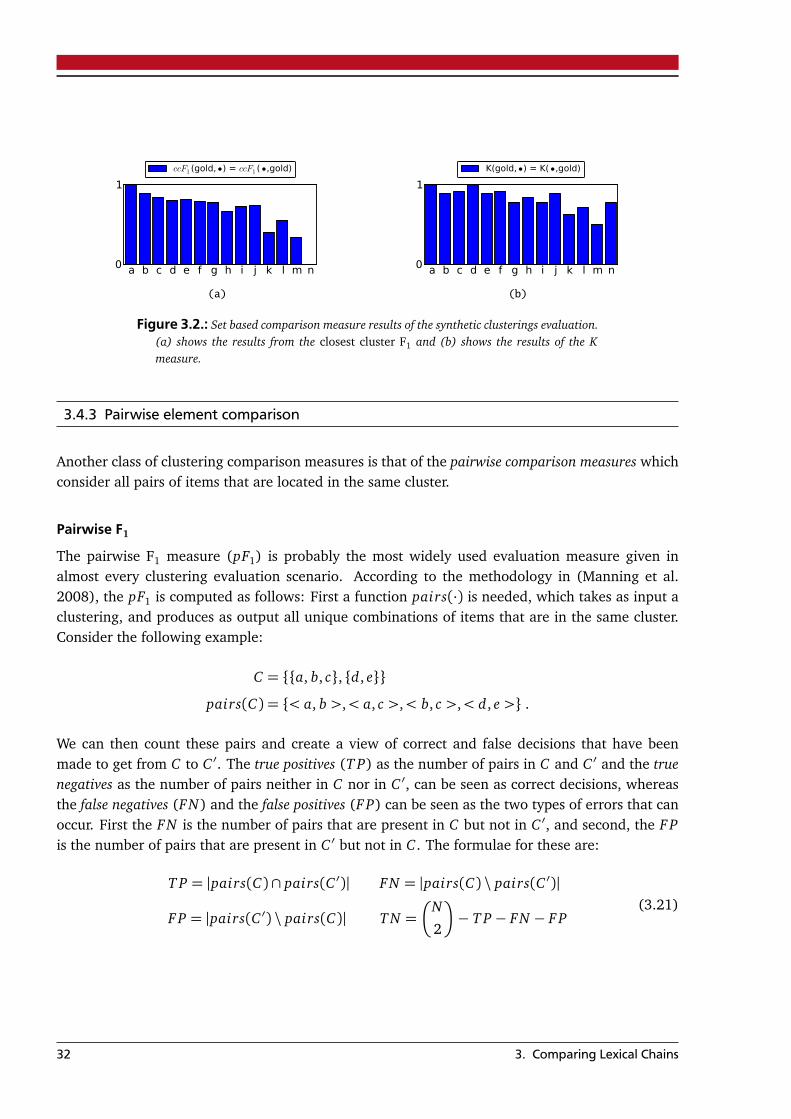
a b c d e f g h i j k l m n0
1
ccF1 (gold, •) = ccF1 ( •,gold)
(a)
a b c d e f g h i j k l m n0
1
K(gold, •) = K( •,gold)
(b)
Figure 3.2.: Set based comparison measure results of the synthetic clusterings evaluation.(a) shows the results from the closest cluster F1 and (b) shows the results of the Kmeasure.
3.4.3 Pairwise element comparison
Another class of clustering comparison measures is that of the pairwise comparison measures whichconsider all pairs of items that are located in the same cluster.
Pairwise F1
The pairwise F1 measure (pF1) is probably the most widely used evaluation measure given inalmost every clustering evaluation scenario. According to the methodology in (Manning et al.2008), the pF1 is computed as follows: First a function pairs(·) is needed, which takes as input aclustering, and produces as output all unique combinations of items that are in the same cluster.Consider the following example:
C = {{a, b, c}, {d, e}}
pairs(C) = {< a, b >,< a, c >,< b, c >,< d, e >} .
We can then count these pairs and create a view of correct and false decisions that have beenmade to get from C to C ′. The true positives (T P) as the number of pairs in C and C ′ and the truenegatives as the number of pairs neither in C nor in C ′, can be seen as correct decisions, whereasthe false negatives (FN) and the false positives (F P) can be seen as the two types of errors that canoccur. First the FN is the number of pairs that are present in C but not in C ′, and second, the F Pis the number of pairs that are present in C ′ but not in C . The formulae for these are:
T P = |pairs(C)∩ pairs(C ′)| FN = |pairs(C) \ pairs(C ′)|
F P = |pairs(C ′) \ pairs(C)| T N =�
N
2
�
− T P − FN − F P(3.21)
32 3. Comparing Lexical Chains
An alternative computation of these values is by means of combinatorics. Using a contingencytable, the T P-, T N -, F P-, and FN -values can be computed as:
T P =∑
i, j
�
ni j
2
�
FN =∑
i
�
ni.
2
�
− T P
F P =∑
j
�
n. j
2
�
− T P T N =�
N
2
�
− T P − FN − F P(3.22)
Finally, pairwise precision (pP), pairwise recall (pR) and pairwise F1 (pF1) is computed as:
pP(C , C ′) =T P
T P + F P(3.23)
pR(C , C ′) =T P
T P + FN(3.24)
pF1(C , C ′) =2× pP(C , C ′)× pR(C , C ′)
pP(C , C ′) + pR(C , C ′)(3.25)
Figure 3.3a shows the results of the synthetic test. The strength of the pF1 measure is that itsuccessfully recognizes and punishes the orthogonal clustering (cf. m) and different datasets (cf.n). The major drawback of pairwise comparison measures can be observed in l, where each item isin a single cluster. Since the computation is based on pairs, it is a natural assumption that clustersshould consist of at least two items. This is assumption does not cohere with the intuitive lexicalchain comparison, because here, single element chains are possible.
Adjusted Rand Index
The adjusted Rand index (Hubert and Arabie 1985) is another measure from the domain of paircomparison measures. It is an advanced version of the Rand index (Rand 1971), which is simplythe accuracy of the correct pairs versus all pairs:
RI(C , C ′) =T P + T N
T P + T N + F P + FN. (3.26)
3.4. Clustering Comparison Measures 33
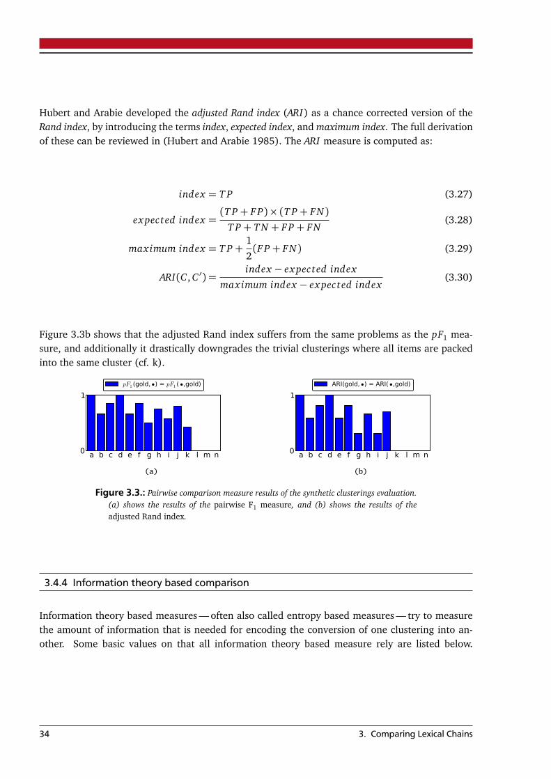
Hubert and Arabie developed the adjusted Rand index (ARI) as a chance corrected version of theRand index, by introducing the terms index, expected index, and maximum index. The full derivationof these can be reviewed in (Hubert and Arabie 1985). The ARI measure is computed as:
index = T P (3.27)
ex pected index =(T P + F P)× (T P + FN)
T P + T N + F P + FN(3.28)
maximum index = T P +1
2(F P + FN) (3.29)
ARI(C , C ′) =index − ex pected index
maximum index − ex pected index(3.30)
Figure 3.3b shows that the adjusted Rand index suffers from the same problems as the pF1 mea-sure, and additionally it drastically downgrades the trivial clusterings where all items are packedinto the same cluster (cf. k).
a b c d e f g h i j k l m n0
1
pF1 (gold, •) = pF1 ( •,gold)
(a)
a b c d e f g h i j k l m n0
1
ARI(gold, •) = ARI( •,gold)
(b)
Figure 3.3.: Pairwise comparison measure results of the synthetic clusterings evaluation.(a) shows the results of the pairwise F1 measure, and (b) shows the results of theadjusted Rand index.
3.4.4 Information theory based comparison
Information theory based measures — often also called entropy based measures — try to measurethe amount of information that is needed for encoding the conversion of one clustering into an-other. Some basic values on that all information theory based measure rely are listed below.
34 3. Comparing Lexical Chains
According to Cover and Thomas (1991), the entropy H(C), the conditional entropy H(C |C ′) andthe mutual information I(C , C ′) are computed as:
H(C) =−∑
i
P(ci) log P(ci) , H(C ′) =−∑
j
P(c′j) log P(c′j) (3.31)
I(C , C ′) =∑
i, j
P(ci, c′j) logP(ci, c′j)
P(ci)P(c′j)(3.32)
H(C |C ′) = H(C)− I(C , C ′) , (3.33)
where the probabilities P(ci) and P(c′j) as well as the joint probability P(ci, c′j) are relative frequen-cies of the contingency table entries:
P(ci) =ni.
N, P(c′j) =
n. j
N, P(ci, c′j) =
ni j
N. (3.34)
LogN Normalized Variation of Information
The variation of information (Meila 2003, 2007) is probably the most prominent information the-oretic measure, which is also proven to be a real metric1. Meila (2005) extensively analyzes andcompares the variation of information metric (V I) with various other measures through some im-portant criteria, and arguments that defacto no measure is able to simultaneously satisfy all ofsome desirable properties, but the variation of information only violates the boundedness property,which says that a measure can be projected into [0,1].
Though the variation of information does not depend on the size of the dataset or the number ofclusters, a normalized version will. Hence Meila proposes two normalization factors: (a) log Nrequiring a fixed size of the dataset, and (b) 2 log K∗ requiring a maximum number of K∗ clustersin C and C ′ and K∗ ≤
pN . Because we cannot assure the number of clusters to be maximally
pN ,
the latter will not be tested here. The V I measure and its log N normalized variant (nNV I) — then stands for naïve, because now the value depends on the size of the dataset, meaning for instancea value of 0.2 on one dataset may be a good value whereas a value of 0.2 on another dataset maybe a rather bad value — is computed as:
V I(C , C ′) = H(C) +H(C ′)− 2I(C , C ′) (3.35)
nNV I(C , C ′) =1
log NV I(C , C ′) . (3.36)
1 a metric is a distance function, which satisfies the following conditions: (a) non-negativity, (b) identity, (c) sym-metry, (d) triangle inequality (Bronstein et al. 2005).
3.4. Clustering Comparison Measures 35
Since the measure is a distance measure, we need to transform it into a similarity measure bysimply using 1− nNV I .
The results of the synthetic tests can be reviewed in Figure 3.4a. The orthogonal clustering in m isrecognized and downweighted by the nNV I measure, but again the clustering in n where no itemsare in common with the clustering in a is valued considerably good opposed to the simple changesin g or i.
Normalized Variation of Information
To overcome the “unboundedness problem” of the V I measure in a more sophisticated way, Re-ichart and Rappoport (2009) proposed the normalized variation of information (NV I), “. . . whichguarantees that the score of clusterings that V I considers good lies in [0,1], regardless of datasetsize”(p. 1).
NV I(C , C ′) =
V I(C , C ′)H(C)
if H(C) 6= 0
H(C ′) otherwise(3.37)
Analogously to nNV I the NV I is a distance measure, which means we use 1− NV I in our com-parison instead.
In Figure 3.4b the results of the synthetic clustering comparisons are depicted. The NVI-measure isnot symmetric, so two values are produced, one for each direction. Note that forcing symmetry canbe easily done here. Nevertheless, additionally to the clustering in m, the NVI measure penalizesthe clustering in k, and like the nNV I it does not recognize the two different datasets in n.
V-Measure
Another measure from the information theory domain based on entropy is the V measure (Vfor validity), which was introduced by Rosenberg and Hirschberg (2007), in order to overcomethe shortcomings of the V I metric. Remember that the main problem is that V I is not bounded.Rosenberg and Hirschberg formulate the V measure in terms of homogeneity and completeness; twocriteria for distinguishing good clustering results from bad ones, that can be directly computed andweighted.
Homogeneity, on one hand, is satisfied if all clusters of a clustering C contain only those elementsthat are also grouped into the same cluster in C ′, and completeness, on the other hand, is satisfiedif all clusters of a clustering in C contain all of the elements that are grouped into the same clusterin C ′. Since homogeneity and completeness are typically diametral, only the perfect clustering
36 3. Comparing Lexical Chains
simultaneously satisfies homogeneity and completeness. Homogeneity (h) and completeness (c)are computed as:
h=
1 if H(C , C ′) = 0
1−H(C |C ′)
H(C)otherwise
, c =
1 if H(C ′, C) = 0
1−H(C ′|C)H(C ′)
otherwise. (3.38)
The V measure is then computed as analogously to the F measure as the weighted harmonic meanof h and c, where the default scenario is equal weights:
V = F1 =2× h× c
h+ c. (3.39)
The main advantage of the V -measure is that the criteria for clustering comparison (i.e. homo-geneity and completeness) are put into numbers. By weighting them, like the F measure does withprecision and recall, it can be configured to best match the task at hand. However, in this the-sis completeness and homogeneity are equally important, and besides to that, unequal weightingof homogeneity and completeness yields V to be asymmetric, which is contrary to the symmetryproperty in Section 3.3.2.
The results of the synthetic test cases are shown in Figure 3.4c. A major problem of the V measureis that it generally favors small clusters (see e.g. Reichart and Rappoport 2009 for a more detaileddiscussion), which can be seen in l and also as an artifact of cluster conformation (Sec. 3.3.1) inn. Another conspicuous thing is that it delivers the exact same results as the normalized mutualinformation, which is described below.
Normalized Mutual Information
Yet another information theory based measure is the normalized variation of information proposedby Strehl (2002). It is a normalized version of the mutual information I(C , C ′) (cf. Eq. (3.32)),which can be seen as the amount of information a clustering C “knows” about another cluster-ing C ′, where it is the reduction in the uncertainty of one clustering due to the knowledge ofthe other (Cover and Thomas 1991). According to Manning et al. (2008) the arithmetic mean[H(C) +H(C ′)]/2 is a tight upper bound on I(C , C ′). Normalizing I(C , C ′) by this factor yields:
N M I(C , C ′) =I(C , C ′)
[H(C) +H(C ′)] / 2=
2 I(C , C ′)H(C) +H(C ′)
. (3.40)
As stated later by Strehl and Ghosh (2003) another possible I(C , C ′) normalization is the geomet-ric mean
p
H(C)H(C ′) instead of the arithmetic mean. Since the difference between these two
3.4. Clustering Comparison Measures 37
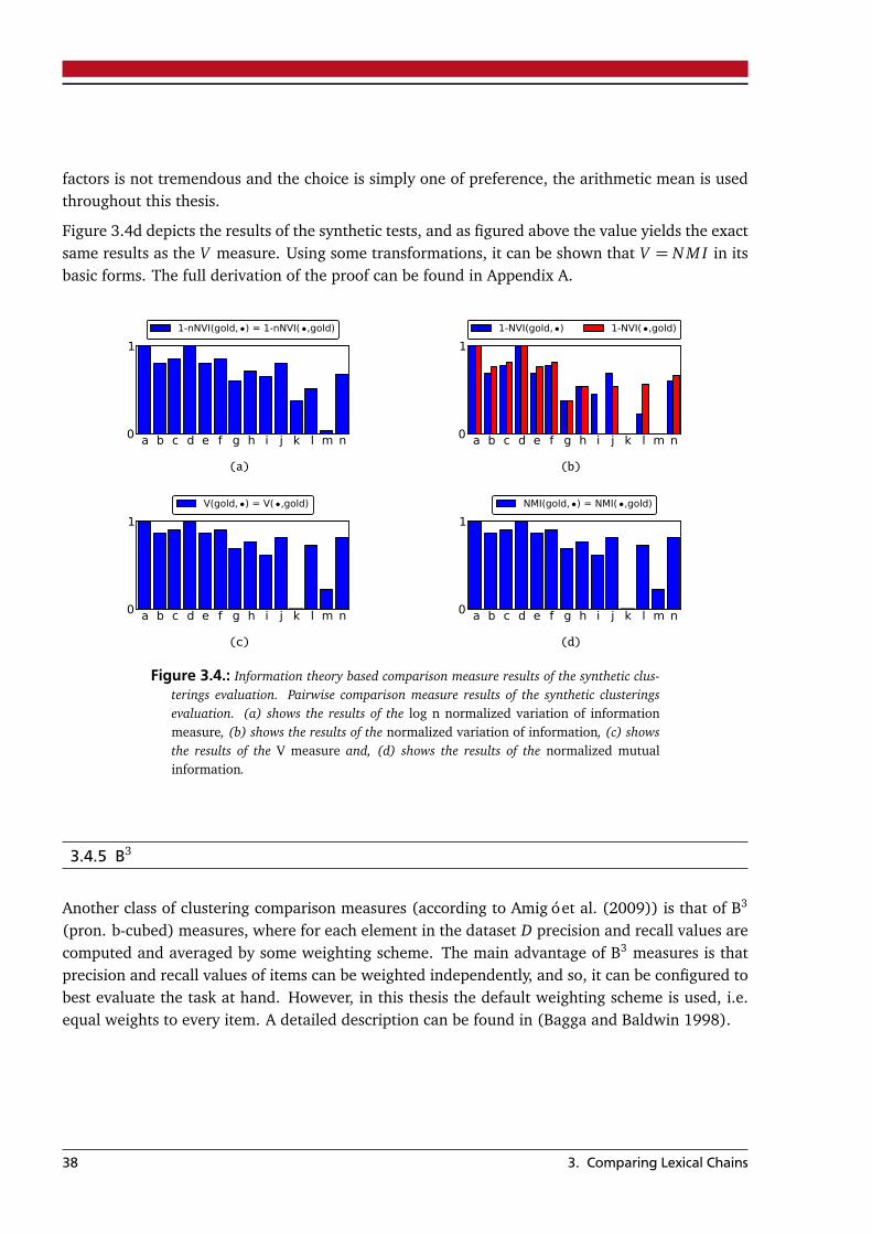
factors is not tremendous and the choice is simply one of preference, the arithmetic mean is usedthroughout this thesis.
Figure 3.4d depicts the results of the synthetic tests, and as figured above the value yields the exactsame results as the V measure. Using some transformations, it can be shown that V = N M I in itsbasic forms. The full derivation of the proof can be found in Appendix A.
a b c d e f g h i j k l m n0
1
1-nNVI(gold, •) = 1-nNVI( •,gold)
(a)
a b c d e f g h i j k l m n0
1
1-NVI(gold, •) 1-NVI( •,gold)
(b)
a b c d e f g h i j k l m n0
1
V(gold, •) = V( •,gold)
(c)
a b c d e f g h i j k l m n0
1
NMI(gold, •) = NMI( •,gold)
(d)
Figure 3.4.: Information theory based comparison measure results of the synthetic clus-terings evaluation. Pairwise comparison measure results of the synthetic clusteringsevaluation. (a) shows the results of the log n normalized variation of informationmeasure, (b) shows the results of the normalized variation of information, (c) showsthe results of the V measure and, (d) shows the results of the normalized mutualinformation.
3.4.5 B3
Another class of clustering comparison measures (according to Amigó et al. (2009)) is that of B3
(pron. b-cubed) measures, where for each element in the dataset D precision and recall values arecomputed and averaged by some weighting scheme. The main advantage of B3 measures is thatprecision and recall values of items can be weighted independently, and so, it can be configured tobest evaluate the task at hand. However, in this thesis the default weighting scheme is used, i.e.equal weights to every item. A detailed description can be found in (Bagga and Baldwin 1998).
38 3. Comparing Lexical Chains
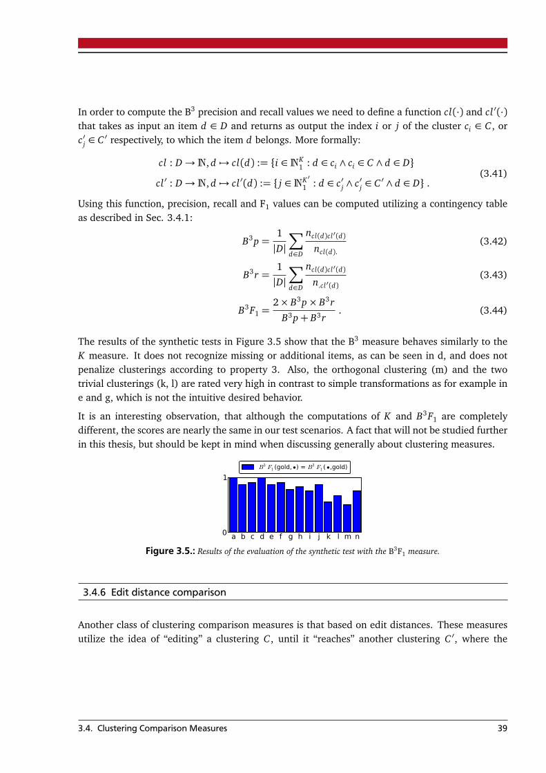
In order to compute the B3 precision and recall values we need to define a function cl(·) and cl ′(·)that takes as input an item d ∈ D and returns as output the index i or j of the cluster ci ∈ C , orc′j ∈ C ′ respectively, to which the item d belongs. More formally:
cl : D→N, d 7→ cl(d) := {i ∈NK1 : d ∈ ci ∧ ci ∈ C ∧ d ∈ D}
cl ′ : D→N, d 7→ cl ′(d) := { j ∈NK′1 : d ∈ c′j ∧ c′j ∈ C ′ ∧ d ∈ D} .
(3.41)
Using this function, precision, recall and F1 values can be computed utilizing a contingency tableas described in Sec. 3.4.1:
B3p =1
|D|
∑
d∈D
ncl(d)cl′(d)
ncl(d).(3.42)
B3r =1
|D|
∑
d∈D
ncl(d)cl′(d)
n.cl′(d)(3.43)
B3F1 =2× B3p× B3r
B3p+ B3r. (3.44)
The results of the synthetic tests in Figure 3.5 show that the B3 measure behaves similarly to theK measure. It does not recognize missing or additional items, as can be seen in d, and does notpenalize clusterings according to property 3. Also, the orthogonal clustering (m) and the twotrivial clusterings (k, l) are rated very high in contrast to simple transformations as for example ine and g, which is not the intuitive desired behavior.
It is an interesting observation, that although the computations of K and B3F1 are completelydifferent, the scores are nearly the same in our test scenarios. A fact that will not be studied furtherin this thesis, but should be kept in mind when discussing generally about clustering measures.
a b c d e f g h i j k l m n0
1
B3 F1 (gold, •) = B3 F1 ( •,gold)
Figure 3.5.: Results of the evaluation of the synthetic test with the B3F1 measure.
3.4.6 Edit distance comparison
Another class of clustering comparison measures is that based on edit distances. These measuresutilize the idea of “editing” a clustering C , until it “reaches” another clustering C ′, where the
3.4. Clustering Comparison Measures 39
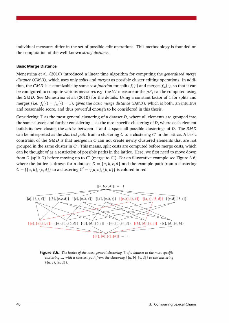
individual measures differ in the set of possible edit operations. This methodology is founded onthe computation of the well-known string distance.
Basic Merge Distance
Menestrina et al. (2010) introduced a linear time algorithm for computing the generalized mergedistance (GM D), which uses only splits and merges as possible cluster editing operations. In addi-tion, the GM D is customizable by some cost function for splits fs(·) and merges fm(·), so that it canbe configured to compute various measures e.g. the V I measure or the pF1 can be computed usingthe GM D. See Menestrina et al. (2010) for the details. Using a constant factor of 1 for splits andmerges (i.e. fs(·) = fm(·) = 1), gives the basic merge distance (BM D), which is both, an intuitiveand reasonable score, and thus powerful enough to be considered in this thesis.
Considering > as the most general clustering of a dataset D, where all elements are grouped intothe same cluster, and further considering⊥ as the most specific clustering of D, where each elementbuilds its own cluster, the lattice between > and ⊥ spans all possible clusterings of D. The BM Dcan be interpreted as the shortest path from a clustering C to a clustering C ′ in the lattice. A basicconstraint of the GM D is that merges in C can not create newly clustered elements that are notgrouped in the same cluster in C ′. This means, split costs are computed before merge costs, whichcan be thought of as a restriction of possible paths in the lattice. Here, we first need to move downfrom C (split C) before moving up to C ′ (merge to C ′). For an illustrative example see Figure 3.6,where the lattice is drawn for a dataset D = {a, b, c, d} and the example path from a clusteringC = {{a, b}, {c, d}} to a clustering C ′ = {{a, c}, {b, d}} is colored in red.
{{a, b, c, d}} = >
{{a}, {b, c, d}} {{b}, {a, c, d}} {{c}, {a, b, d}} {{d}, {a, b, c}} {{a, b}, {c, d}} {{a, c}, {b, d}} {{a, d}, {b, c}}
{{a}, {b}, {c, d}} {{a}, {c}, {b, d}} {{a}, {d}, {b, c}} {{b}, {c}, {a, d}} {{b}, {d}, {a, c}} {{c}, {d}, {a, b}}
{{a}, {b}, {c}, {d}} = ⊥
Figure 3.6.: The lattice of the most general clustering > of a dataset to the most specificclustering ⊥, with a shortest path from the clustering {{a, b}, {c, d}} to the clustering{{a, c}, {b, d}}.
40 3. Comparing Lexical Chains
Formalizing the BM D in terms of the GM D according to Menestrina et al. (2010) yields the fol-lowing definition:
BM D(C , C ′) = GM D fs , fm(C , C ′) (3.45)
fs(|X |, |Y |) = 1 , fm(|X |, |Y |) = 1 , (3.46)
where X and Y are two connected clusterings on the lattice, and fs and fm are the cost functionsfor splitting X into Y or merging X into Y respectively.
Normalized Basic Merge Distance
The value of the BM D now describes how many operations are needed to get from a clustering C toa clustering C ′ in a natural and intuitive way, but in order to be conform with property 1 in Section3.3.2 we need to normalize it to lie in [0,1]. The resulting measure is then called normalized basicmerge distance (NBM D). One option to get compute the nBM D is to divide it by the maximumvalue the BM D can become for the current underlying dataset:
NBM D(C , C ′) =BM D(C , C ′)
max(BM D(C , C ′))(3.47)
Clearly, the maximum number of operations is the maximum shortest distance of two clusterings inthe lattice. Let N be the number of elements in a dataset D, it can be shown that for any clusteringsC and C ′ of the dataset D:
max(BM D(C , C ′)) =
¨
BM D(>,⊥) if 1≤ N ≤ 31+ BM D(>,⊥) if N > 3
, (3.48)
which is equivalent to:
max(BM D(C , C ′)) =
0 if N = 1N − 1 if 1< N ≤ 3
N if N > 3. (3.49)
Since the NBM D is a distance value, 1− NBM D is used instead. By normalizing with the max-imum, the NBM D measure is now dependent on the size of the dataset, as is the nNV I , whichmeans the value is now hardly interpretable when comparing the results of two datasets.
Figure 3.7a shows the behavior of the measure when computing closeness between the syntheticclusterings described in Figure 3.1. The high values in d and n show that the value suffers from the
3.4. Clustering Comparison Measures 41
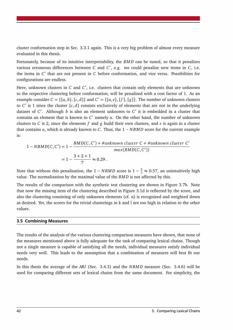
cluster conformation step in Sec. 3.3.1 again. This is a very big problem of almost every measureevaluated in this thesis.
Fortunately, because of its intuitive interpretability, the BM D can be tuned, so that it penalizesvarious erroneous differences between C and C ′, e.g. we could penalize new items in C , i.e.the items in C ′ that are not present in C before conformation, and vice versa. Possibilities forconfigurations are endless.
Here, unknown clusters in C and C ′, i.e. clusters that contain only elements that are unknownto the respective clustering before conformation, will be penalized with a cost factor of 1. As anexample consider C = {{a, b}, {c, d}} and C ′ = {{a, e}, { f }, {g}}. The number of unknown clustersto C ′ is 1 since the cluster {c, d} consists exclusively of elements that are not in the underlyingdataset of C ′. Although b is also an element unknown to C ′ it is embedded in a cluster thatcontains an element that is known to C ′ namely a. On the other hand, the number of unknownclusters to C is 2, since the elements f and g build their own clusters, and e is again in a clusterthat contains a, which is already known to C . Thus, the 1− NBM D score for the current exampleis:
1− NBM D(C , C ′) = 1−BM D(C , C ′) +#unknown cluster C +#unknown cluster C ′
max(BM D(C , C ′))
= 1−3+ 2+ 1
7≈ 0.29 .
Note that without this penalization, the 1− NBM D score is 1− 37≈ 0.57, an unintuitively high
value. The normalization by the maximal value of the BM D is not affected by this.
The results of the comparison with the synthetic test clustering are shown in Figure 3.7b. Notethat now the missing item of the clustering described in Figure 3.1d is reflected by the score, andalso the clustering consisting of only unknown elements (cf. n) is recognized and weighted downas desired. Yet, the scores for the trivial clusterings in k and l are too high in relation to the othervalues.
3.5 Combining Measures
The results of the analysis of the various clustering comparison measures have shown, that none ofthe measures mentioned above is fully adequate for the task of comparing lexical chains. Thoughnot a single measure is capable of satisfying all the needs, individual measures satisfy individualneeds very well. This leads to the assumption that a combination of measures will best fit ourneeds.
In this thesis the average of the ARI (Sec. 3.4.3) and the NBM D measure (Sec. 3.4.6) will beused for comparing different sets of lexical chains from the same document. For simplicity, the
42 3. Comparing Lexical Chains
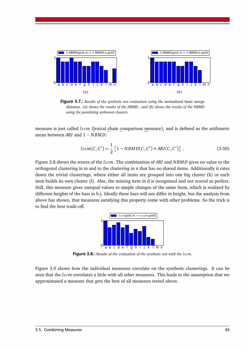
a b c d e f g h i j k l m n0
1
1-NBMD(gold, •) = 1-NBMD( •,gold)
(a)
a b c d e f g h i j k l m n0
1
1-NBMD(gold, •) = 1-NBMD( •,gold)
(b)
Figure 3.7.: Results of the synthetic test evaluation using the normalized basic mergedistance. (a) shows the results of the NBMD , and (b) shows the results of the NBMDusing the penalizing unknown clusters.
measure is just called lccm (lexical chain comparison measure), and is defined as the arithmeticmean between ARI and 1− NBM D:
lccm(C , C ′) =1
2
�
1− NBM D(C , C ′) + ARI(C , C ′)�
. (3.50)
Figure 3.8 shows the scores of the lccm. The combination of ARI and NBM D gives no value to theorthogonal clustering in m and to the clustering in n that has no shared items. Additionally it ratesdown the trivial clusterings, where either all items are grouped into one big cluster (k) or eachitem builds its own cluster (l). Also, the missing item in d is recognized and not scored as perfect.Still, this measure gives unequal values to simple changes of the same form, which is realized bydifferent heights of the bars in b-j. Ideally these bars will not differ in height, but the analysis fromabove has shown, that measures satisfying this property come with other problems. So the trick isto find the best trade-off.
a b c d e f g h i j k l m n0
1
lccm(gold, •) = lccm( •,gold)
Figure 3.8.: Results of the evaluation of the synthetic test with the lccm.
Figure 3.9 shows how the individual measures correlate on the synthetic clusterings. It can beseen that the lccm correlates a little with all other measures. This leads to the assumption that weapproximated a measure that gets the best of all measures tested above.
3.5. Combining Measures 43
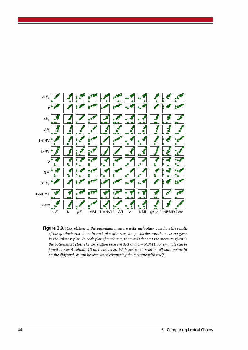
ccF1
K
pF1
ARI
1-nNVI
1-NVI
V
NMI
B3 F1
1-NBMD
ccF1
lccm
K pF1 ARI 1-nNVI 1-NVI V NMI B3 F11-NBMD lccm
Figure 3.9.: Correlation of the individual measure with each other based on the resultsof the synthetic test data. In each plot of a row, the y-axis denotes the measure givenin the leftmost plot. In each plot of a column, the x-axis denotes the measure given inthe bottommost plot. The correlation between ARI and 1− NBM D for example can befound in row 4 column 10 and vice versa. With perfect correlation all data points lieon the diagonal, as can be seen when comparing the measure with itself.
44 3. Comparing Lexical Chains
4 Annotating Lexical ChainsText, annotated with lexical chain information is a must-have for many reasons. It can be usedeither to analyze lexical cohesion in more detail (cf. for example Teich and Fankhauser 2005) inorder to build better chaining algorithm, or it can be used for training a supervised lexical chainingalgorithm, or, and this is probably the greatest desire, it can be used to qualitatively compare lexicalchains of a particular document from many annotating sources, i.e. inter-annotator agreement andevaluation of automatic approaches. Creating such a gold standard allows researchers to test theirimplementation individually on a common basis. This practice is generally applied (if possible)in the machine learning area where a high agreement in annotated data is required otherwise themethod is not considered to be reliable (Morris 2010).
Unfortunately, the annotation of lexical chains is highly influenced by the subjective interpretationof the text by individual annotators (Morris and Hirst 2004) which also substantiates the fact thatcurrently no gold standard exists. Morris (2010) noted that the difference in interpretation is ap-proximately 40% and that high inter-annotator agreement is extremely hard to achieve and — dueto natural human text interpretation — is either not possible or just the result of unnaturally forcedinterpretation scenarios.
Nevertheless, Hollingsworth and Teufel (2005) as well as Cramer et al. (2008) experimented withthe annotation of lexical chains; both concluding with the same result that high inter-annotatoragreement cannot be achieved.
In the context of this thesis an annotation project was carried out in which a corpus was annotatedwith lexical chain information. One hundred general domain news articles from a German news-paper were annotated by two annotators. The next sections describe the underlying corpus andthe applied methodology as well as the toolkit used.
4.1 Corpus
In this thesis the documents of the SALSA1 2.0 (Burchardt et al. 2006) corpus were chosen toform the basis for the annotation of lexical chain information. SALSA 2.0 itself is based on thesemi-automatically annotated TIGER Treebank 2.1 (Brants et al. 2002). Salsa already provides in-
1 SALSA II - The Saarbrücken Lexical Semantics Acquisition Project
45
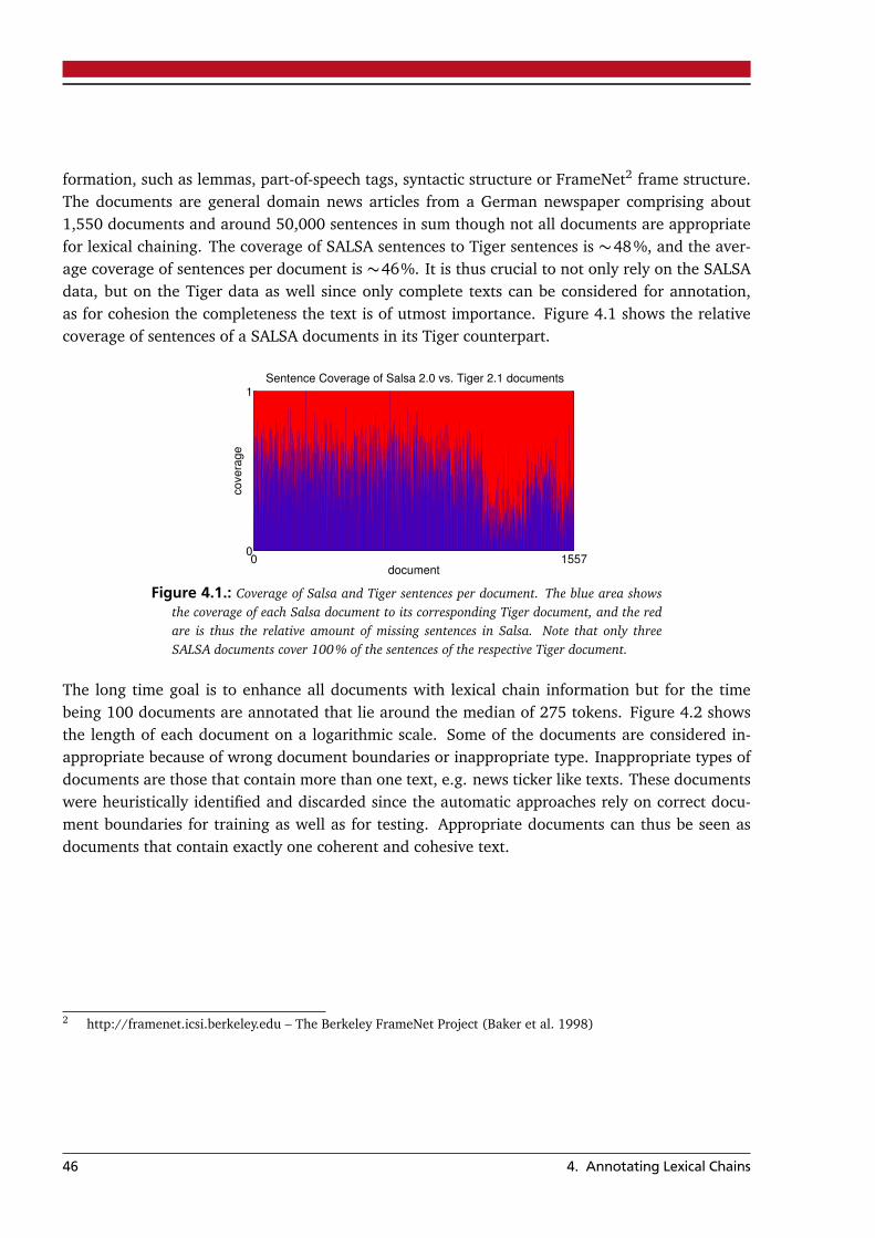
formation, such as lemmas, part-of-speech tags, syntactic structure or FrameNet2 frame structure.The documents are general domain news articles from a German newspaper comprising about1,550 documents and around 50,000 sentences in sum though not all documents are appropriatefor lexical chaining. The coverage of SALSA sentences to Tiger sentences is ∼48%, and the aver-age coverage of sentences per document is ∼46%. It is thus crucial to not only rely on the SALSAdata, but on the Tiger data as well since only complete texts can be considered for annotation,as for cohesion the completeness the text is of utmost importance. Figure 4.1 shows the relativecoverage of sentences of a SALSA documents in its Tiger counterpart.
0 15570
1Sentence Coverage of Salsa 2.0 vs. Tiger 2.1 documents
document
covera
ge
Figure 4.1.: Coverage of Salsa and Tiger sentences per document. The blue area showsthe coverage of each Salsa document to its corresponding Tiger document, and the redare is thus the relative amount of missing sentences in Salsa. Note that only threeSALSA documents cover 100% of the sentences of the respective Tiger document.
The long time goal is to enhance all documents with lexical chain information but for the timebeing 100 documents are annotated that lie around the median of 275 tokens. Figure 4.2 showsthe length of each document on a logarithmic scale. Some of the documents are considered in-appropriate because of wrong document boundaries or inappropriate type. Inappropriate types ofdocuments are those that contain more than one text, e.g. news ticker like texts. These documentswere heuristically identified and discarded since the automatic approaches rely on correct docu-ment boundaries for training as well as for testing. Appropriate documents can thus be seen asdocuments that contain exactly one coherent and cohesive text.
2 http://framenet.icsi.berkeley.edu – The Berkeley FrameNet Project (Baker et al. 1998)
46 4. Annotating Lexical Chains
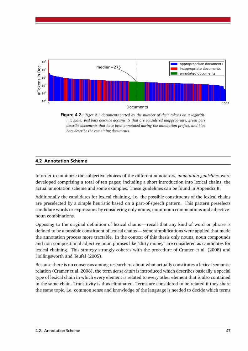
0 1557
Documents
100
101
102
103
104
105
#Toke
ns
in D
oc. median=275
appropropriate documents
inappropriate documents
annotated documents
Figure 4.2.: Tiger 2.1 documents sorted by the number of their tokens on a logarith-mic scale. Red bars describe documents that are considered inappropriate, green barsdescribe documents that have been annotated during the annotation project, and bluebars describe the remaining documents.
4.2 Annotation Scheme
In order to minimize the subjective choices of the different annotators, annotation guidelines weredeveloped comprising a total of ten pages; including a short introduction into lexical chains, theactual annotation scheme and some examples. These guidelines can be found in Appendix B.
Additionally the candidates for lexical chaining, i.e. the possible constituents of the lexical chainsare preselected by a simple heuristic based on a part-of-speech pattern. This pattern preselectscandidate words or expressions by considering only nouns, noun-noun combinations and adjective-noun combinations.
Opposing to the original definition of lexical chains — recall that any kind of word or phrase isdefined to be a possible constituent of lexical chains — some simplifications were applied that madethe annotation process more tractable. In the context of this thesis only nouns, noun compoundsand non-compositional adjective noun phrases like “dirty money” are considered as candidates forlexical chaining. This strategy strongly coheres with the procedure of Cramer et al. (2008) andHollingsworth and Teufel (2005).
Because there is no consensus among researchers about what actually constitutes a lexical semanticrelation (Cramer et al. 2008), the term dense chain is introduced which describes basically a specialtype of lexical chain in which every element is related to every other element that is also containedin the same chain. Transitivity is thus eliminated. Terms are considered to be related if they sharethe same topic, i.e. common sense and knowledge of the language is needed to decide which terms
4.2. Annotation Scheme 47
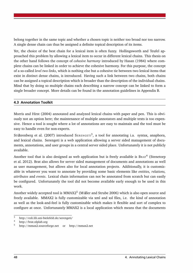
belong together in the same topic and whether a chosen topic is neither too broad nor too narrow.A single dense chain can thus be assigned a definite topical description of its items.
Yet, the choice of the best chain for a lexical item is often fuzzy. Hollingsworth and Teufel ap-proached this problem by allowing a lexical item to occur in different lexical chains. This thesis onthe other hand follows the concept of cohesive harmony introduced by Hasan (1984) where com-plete chains can be linked in order to achieve the cohesive harmony. For this purpose, the conceptof a so-called level two links, which is nothing else but a cohesive tie between two lexical items thatexist in distinct dense chains, is introduced. Having such a link between two chains, both chainscan be assigned a topical description which is broader than the description of the individual chains.Mind that by doing so multiple chains each describing a narrow concept can be linked to form asingle broader concept. More details can be found in the annotation guidelines in Appendix B.
4.3 Annotation Toolkit
Morris and Hirst (2004) annotated and analyzed lexical chains with paper and pen. This is obvi-ously not an option here; the maintenance of multiple annotators and multiple texts is too expen-sive. Hence a tool is sought where a lot of annotations are easy to maintain and the tool must beeasy to handle even for non-experts.
Stührenberg et al. (2007) introduced SERENGETI3, a tool for annotating i.a. syntax, anaphora,and lexical chains. Serengeti is a web application allowing a server sided management of docu-ments, annotations, and user groups in a central server sided place. Unfortunately it is not publiclyavailable.
Another tool that is also designed as web application but is freely available is BRAT4 (Stenetorpet al. 2012). Brat also allows for server sided management of documents and annotations as wellas user management, but allows also for local annotation projects. Additionally, it is customiz-able in whatever you want to annotate by providing some basic elements like entities, relations,attributes and events. Lexical chain information can not be annotated from scratch but can easilybe configured. Unfortunately the tool did not become available early enough to be used in thiswork.
Another widely accepted tool is MMAX25 (Müller and Strube 2006) which is also open source andfreely available. MMAX2 is fully customizable via xml and xsl files, i.e. the kind of annotationas well as the look-and-feel is fully customizable which makes it flexible and sort of complex toconfigure at once. Unfortunately MMAX2 is a local application which means that the documents
3 http://coli.lili.uni-bielefeld.de/serengeti/4 http://brat.nlplab.org5 http://mmax2.sourceforge.net or http://mmax2.net
48 4. Annotating Lexical Chains
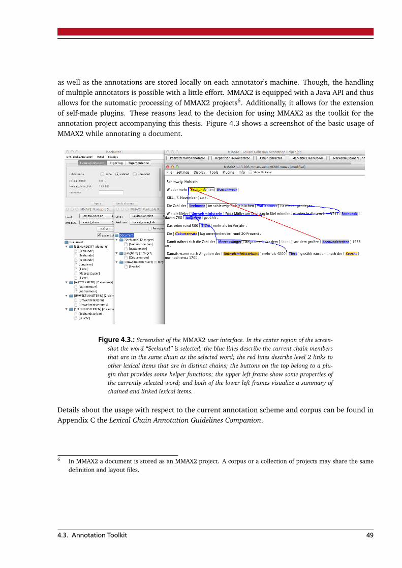
as well as the annotations are stored locally on each annotator’s machine. Though, the handlingof multiple annotators is possible with a little effort. MMAX2 is equipped with a Java API and thusallows for the automatic processing of MMAX2 projects6. Additionally, it allows for the extensionof self-made plugins. These reasons lead to the decision for using MMAX2 as the toolkit for theannotation project accompanying this thesis. Figure 4.3 shows a screenshot of the basic usage ofMMAX2 while annotating a document.
Figure 4.3.: Screenshot of the MMAX2 user interface. In the center region of the screen-shot the word “Seehund” is selected; the blue lines describe the current chain membersthat are in the same chain as the selected word; the red lines describe level 2 links toother lexical items that are in distinct chains; the buttons on the top belong to a plu-gin that provides some helper functions; the upper left frame show some properties ofthe currently selected word; and both of the lower left frames visualize a summary ofchained and linked lexical items.
Details about the usage with respect to the current annotation scheme and corpus can be found inAppendix C the Lexical Chain Annotation Guidelines Companion.
6 In MMAX2 a document is stored as an MMAX2 project. A corpus or a collection of projects may share the samedefinition and layout files.
4.3. Annotation Toolkit 49
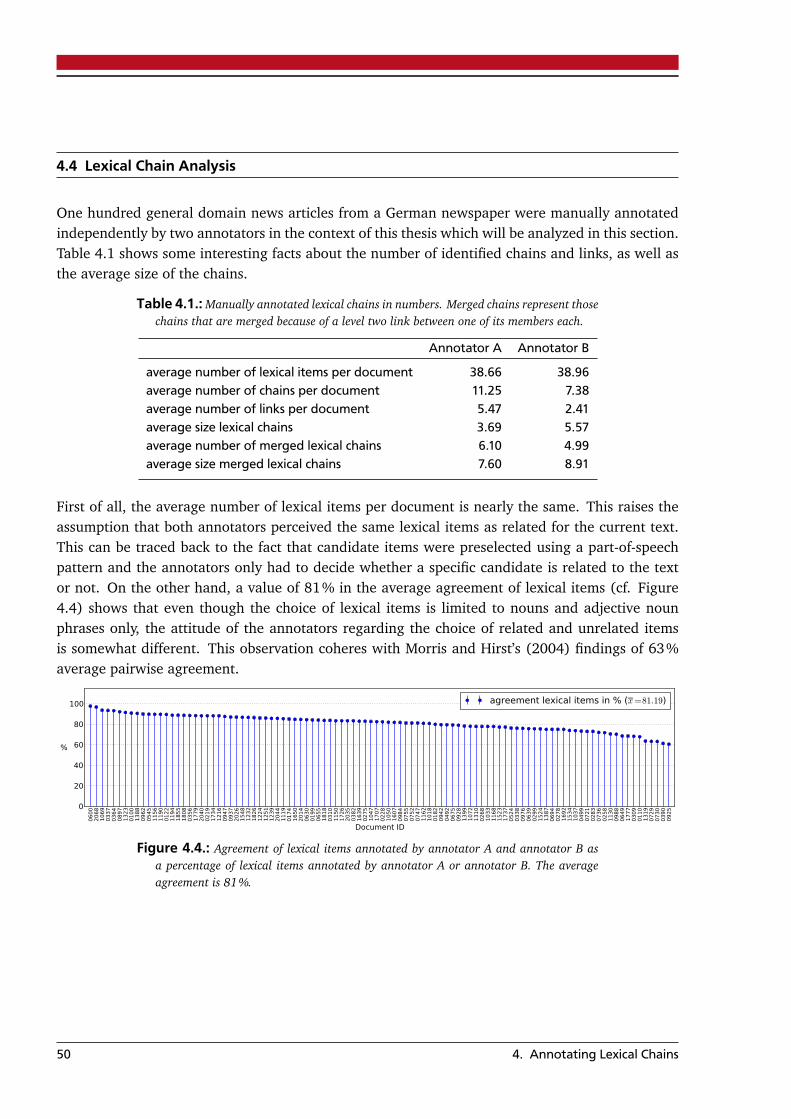
4.4 Lexical Chain Analysis
One hundred general domain news articles from a German newspaper were manually annotatedindependently by two annotators in the context of this thesis which will be analyzed in this section.Table 4.1 shows some interesting facts about the number of identified chains and links, as well asthe average size of the chains.
Table 4.1.: Manually annotated lexical chains in numbers. Merged chains represent thosechains that are merged because of a level two link between one of its members each.
Annotator A Annotator B
average number of lexical items per document 38.66 38.96average number of chains per document 11.25 7.38average number of links per document 5.47 2.41average size lexical chains 3.69 5.57average number of merged lexical chains 6.10 4.99average size merged lexical chains 7.60 8.91
First of all, the average number of lexical items per document is nearly the same. This raises theassumption that both annotators perceived the same lexical items as related for the current text.This can be traced back to the fact that candidate items were preselected using a part-of-speechpattern and the annotators only had to decide whether a specific candidate is related to the textor not. On the other hand, a value of 81% in the average agreement of lexical items (cf. Figure4.4) shows that even though the choice of lexical items is limited to nouns and adjective nounphrases only, the attitude of the annotators regarding the choice of related and unrelated itemsis somewhat different. This observation coheres with Morris and Hirst’s (2004) findings of 63%average pairwise agreement.
06
00
20
68
10
69
03
37
03
64
08
97
13
23
01
00
13
88
09
62
05
45
11
56
11
90
01
22
11
94
18
55
18
08
03
56
17
79
20
40
02
19
17
34
12
16
09
47
09
37
20
26
15
48
12
32
18
26
12
24
12
51
12
39
20
44
11
19
01
74
16
50
20
14
06
30
01
99
06
55
18
18
03
10
11
50
17
26
20
35
03
82
16
39
02
75
10
47
17
07
02
28
10
50
16
07
09
84
07
55
07
52
07
47
11
62
10
18
01
82
09
42
04
92
06
75
09
28
13
99
10
72
13
10
02
68
10
33
11
68
15
23
17
37
05
24
03
38
09
76
06
39
02
99
15
24
13
87
06
94
02
78
16
92
15
34
10
37
04
99
07
21
02
83
07
36
02
58
11
30
09
88
06
49
17
77
03
09
01
10
13
19
07
29
07
30
03
90
09
25
Document ID
0
20
40
60
80
100
%
agreement lexical items in % (x=81.19)
Figure 4.4.: Agreement of lexical items annotated by annotator A and annotator B asa percentage of lexical items annotated by annotator A or annotator B. The averageagreement is 81%.
50 4. Annotating Lexical Chains
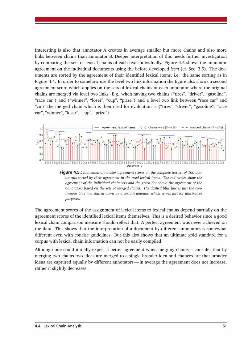
Interesting is also that annotator A creates in average smaller but more chains and also morelinks between chains than annotator B. Deeper interpretation of this needs further investigationby comparing the sets of lexical chains of each text individually. Figure 4.5 shows the annotatoragreement on the individual documents using the before developed lccm (cf. Sec. 3.5). The doc-uments are sorted by the agreement of their identified lexical items, i.e. the same sorting as inFigure 4.4. In order to somehow use the level two link information the figure also shows a secondagreement score which applies on the sets of lexical chains of each annotator where the originalchains are merged via level two links. E.g. when having two chains {“tires”, “driver”, “gasoline”,“race car”} and {“winner”, “loser”, “cup”, “prize”} and a level two link between “race car” and“cup” the merged chain which is then used for evaluation is {“tires”, “driver”, “gasoline”, “racecar”, “winner”, “loser”, “cup”, “prize”}.
06
00
20
68
10
69
03
37
03
64
08
97
13
23
01
00
13
88
09
62
05
45
11
56
11
90
01
22
11
94
18
55
18
08
03
56
17
79
20
40
02
19
17
34
12
16
09
47
09
37
20
26
15
48
12
32
18
26
12
24
12
51
12
39
20
44
11
19
01
74
16
50
20
14
06
30
01
99
06
55
18
18
03
10
11
50
17
26
20
35
03
82
16
39
02
75
10
47
17
07
02
28
10
50
16
07
09
84
07
55
07
52
07
47
11
62
10
18
01
82
09
42
04
92
06
75
09
28
13
99
10
72
13
10
02
68
10
33
11
68
15
23
17
37
05
24
03
38
09
76
06
39
02
99
15
24
13
87
06
94
02
78
16
92
15
34
10
37
04
99
07
21
02
83
07
36
02
58
11
30
09
88
06
49
17
77
03
09
01
10
13
19
07
29
07
30
03
90
09
25
Document ID
0.0
0.2
0.4
0.6
0.8
1.0
lccm
agreement lexical items chains only (x=0.56) merged chains (x=0.54)
Figure 4.5.: Individual annotator agreement scores on the complete test set of 100 doc-uments sorted by their agreement in the used lexical items. The red circles show theagreement of the individual chain sets and the green dot shows the agreement of theannotators based on the sets of merged chains. The dashed blue line is just the con-tinuous blue line shifted down by a certain amount, which serves just for illustrativepurposes.
The agreement scores of the assignment of lexical items to lexical chains depend partially on theagreement scores of the identified lexical items themselves. This is a desired behavior since a goodlexical chain comparison measure should reflect that. A perfect agreement was never achieved onthe data. This shows that the interpretation of a document by different annotators is somewhatdifferent even with concise guidelines. But this also shows that an ultimate gold standard for acorpus with lexical chain information can not be easily compiled.
Although one could initially expect a better agreement when merging chains — consider that bymerging two chains two ideas are merged to a single broader idea and chances are that broaderideas are captured equally by different annotators — in average the agreement does not increase,rather it slightly decreases.
4.4. Lexical Chain Analysis 51

52 4. Annotating Lexical Chains
5 Statistical Methods for Lexical ChainingWith growing computational power and even more available data more and more methods emergeor revive that exploit statistical assumptions about natural language. According to the “law of largenumbers” statistics shows its full strength once enough data is available and moreover processable.In earlier works the input data is often restrained due to technical limitations in time and space,but the faster the computations become and the more data can be accessed efficiently, the moredata can be processed in the same period and the more accurate and authentic the results become.
Most statistical tests in natural language processing are based on the occurrence and co-occurrenceof terms in the same document, paragraph, sentence, n-gram, or the like. This thesis employs twowell-studied statistical methods for creating something that Barzilay (1997) called an automaticthesaurus which will then be adapted for lexical chaining.
5.1 Candidate Lexical Items
A candidate lexical item is a word or phrase that will be eventually inserted into a lexical chainor not. In the following, candidate lexical items are preselected in a text by the same heuristicthat is also applied in Chapter 4 for the simplification of the annotation process. The heuristicis a regular expression working on patterns of the part-of-speech of the words which preselectsall nouns, noun-noun combinations, adjective-noun combinations as well as adjective-noun-nouncombinations. This way, the heuristic tries to identify meaningful noun compounds and non-compositional adjective noun phrases. As an example consider the sentence in 5.1.
( 5.1 ) The child called for an exciting bedtime story.
Here, the following words and phrases are considered as possible candidate lexical items: {“child”,“story”, “bedtime story”, “exciting bedtime”, “exciting bedtime story”}.
5.2 Probabilistic Topic Models
Topic models (TMs) are a suite of unsupervised algorithms designed for unveiling some hiddenstructure in large data collections. The basic assumption of TMs is that there exists at least somelatent theme in the data that actually generated it. In natural language processing, the data is often
53
represented as document-term matrix where rows are documents, columns are vocabulary terms,and the value in a specific row and column represents the number of occurrences of the term inthe document. The key idea is that documents can be represented as composites of so-called topicswhere a topic itself represents as a composite of words. Still, TMs are not bound to documentsand terms — although the name might suggest that — they are more generally applicable to anykind of discrete data. The word “topic” simply emerged because these algorithms, when appliedon language data, deliver results that remind one of groups of related terms that share the sametopic (Blei et al. 2003).
Topic models have its origin in the psychology community where the assumption is that the ap-plication to large datasets can yield insights into human cognition (Steyvers and Griffiths 2006).It all began with latent semantic analysis (LSA) (Deerwester et al. 1990) — in the information re-trieval community also known as latent semantic indexing (LSI) — which is not yet a topic modelthough highly related to the development of these. The LSA method is based on simple linearalgebra: Documents and words are represented as points in the Euclidean space. By applying ma-trix factorization a lower dimensional view of the training data is created that might reveal someshared structure such as synonymy or polysemy. Unseen documents can then also be transformedinto a lower dimensional view by multiplying with these factors.
When Hofmann (1999a, 1999b) published probabilistic latent semantic analysis (pLSA) — alsoknown as probabilistic latent semantic indexing (pLSI) or the aspect model — he introduced a solidstatistical foundation and a proper definition of a generative data model which reveals similar in-formation like LSA but with the values being intuitively interpretable. This makes pLSA the firsttrue topic model. Here, a topic is defined to be a probability distribution over words and a docu-ment is defined to be a probability distribution over a fixed set of topics. A word w in a documentd is then generated by a statistical mixture model which can be represented as:
P(w, d) = P(d)P(w|d) , with (5.1)
P(w|d) =T∑
i=1
P(w|zi)P(zi|d) , (5.2)
where T is the number of topics, P(w|zi) is the probability of the word w being generated by topiczi and P(zi|d) is the probability of topic zi for the current document d. Note however, that z isa latent variable which is unknown. Further, by generating the observation pairs (w, d) indepen-dently the bag-of-words assumption is applied which says that the order of words in a document isunimportant. Hofmann also provides a MAP estimate for P(w|z), P(d|z) and P(z)— consider thatby applying Baye’s rule P(w, d) can be rewritten as
∑Ti=1 P(zi)P(w|zi)P(d|zi).
However, as noted by Blei et al. (2003) this estimate does not capture unseen documents; it learnsthe topic mixtures only for the documents it is trained on. Hence, they introduced another TM
54 5. Statistical Methods for Lexical Chaining
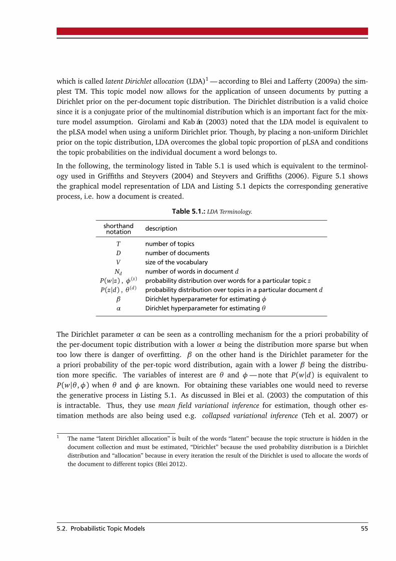
which is called latent Dirichlet allocation (LDA)1 — according to Blei and Lafferty (2009a) the sim-plest TM. This topic model now allows for the application of unseen documents by putting aDirichlet prior on the per-document topic distribution. The Dirichlet distribution is a valid choicesince it is a conjugate prior of the multinomial distribution which is an important fact for the mix-ture model assumption. Girolami and Kabán (2003) noted that the LDA model is equivalent tothe pLSA model when using a uniform Dirichlet prior. Though, by placing a non-uniform Dirichletprior on the topic distribution, LDA overcomes the global topic proportion of pLSA and conditionsthe topic probabilities on the individual document a word belongs to.
In the following, the terminology listed in Table 5.1 is used which is equivalent to the terminol-ogy used in Griffiths and Steyvers (2004) and Steyvers and Griffiths (2006). Figure 5.1 showsthe graphical model representation of LDA and Listing 5.1 depicts the corresponding generativeprocess, i.e. how a document is created.
Table 5.1.: LDA Terminology.
shorthandnotation description
T number of topicsD number of documentsV size of the vocabularyNd number of words in document d
P(w|z) , φ(z) probability distribution over words for a particular topic zP(z|d) , θ (d) probability distribution over topics in a particular document d
β Dirichlet hyperparameter for estimating φα Dirichlet hyperparameter for estimating θ
The Dirichlet parameter α can be seen as a controlling mechanism for the a priori probability ofthe per-document topic distribution with a lower α being the distribution more sparse but whentoo low there is danger of overfitting. β on the other hand is the Dirichlet parameter for thea priori probability of the per-topic word distribution, again with a lower β being the distribu-tion more specific. The variables of interest are θ and φ— note that P(w|d) is equivalent toP(w|θ ,φ) when θ and φ are known. For obtaining these variables one would need to reversethe generative process in Listing 5.1. As discussed in Blei et al. (2003) the computation of thisis intractable. Thus, they use mean field variational inference for estimation, though other es-timation methods are also being used e.g. collapsed variational inference (Teh et al. 2007) or
1 The name “latent Dirichlet allocation” is built of the words “latent” because the topic structure is hidden in thedocument collection and must be estimated, “Dirichlet” because the used probability distribution is a Dirichletdistribution and “allocation” because in every iteration the result of the Dirichlet is used to allocate the words ofthe document to different topics (Blei 2012).
5.2. Probabilistic Topic Models 55
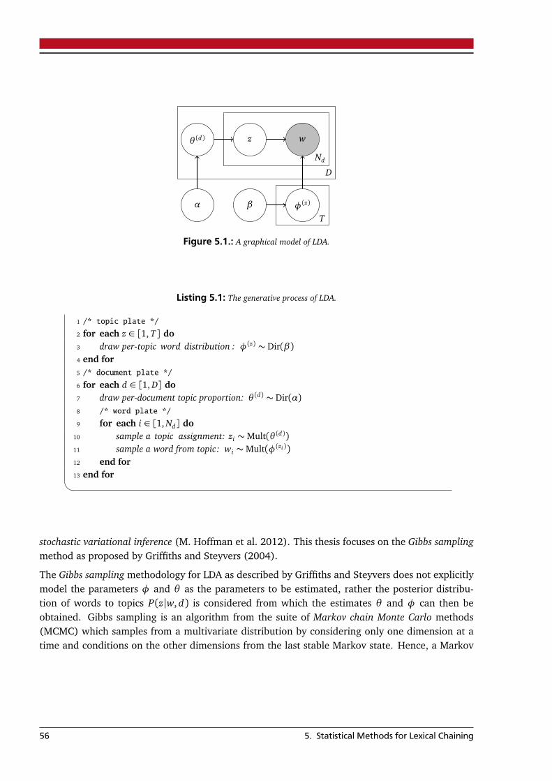
β φ(z)
T
wz
Nd
θ (d)
D
α
Figure 5.1.: A graphical model of LDA.
Listing 5.1: The generative process of LDA.
1 /* topic plate */
2 for each z ∈ [1, T] do3 draw per-topic word distribution : φ(z) ∼ Dir(β)4 end for5 /* document plate */
6 for each d ∈ [1, D] do7 draw per-document topic proportion: θ (d) ∼ Dir(α)8 /* word plate */
9 for each i ∈ [1, Nd] do10 sample a topic assignment: zi ∼Mult(θ (d))11 sample a word from topic: wi ∼Mult(φ(zi))12 end for13 end for�
stochastic variational inference (M. Hoffman et al. 2012). This thesis focuses on the Gibbs samplingmethod as proposed by Griffiths and Steyvers (2004).
The Gibbs sampling methodology for LDA as described by Griffiths and Steyvers does not explicitlymodel the parameters φ and θ as the parameters to be estimated, rather the posterior distribu-tion of words to topics P(z|w, d) is considered from which the estimates θ and φ can then beobtained. Gibbs sampling is an algorithm from the suite of Markov chain Monte Carlo methods(MCMC) which samples from a multivariate distribution by considering only one dimension at atime and conditions on the other dimensions from the last stable Markov state. Hence, a Markov
56 5. Statistical Methods for Lexical Chaining
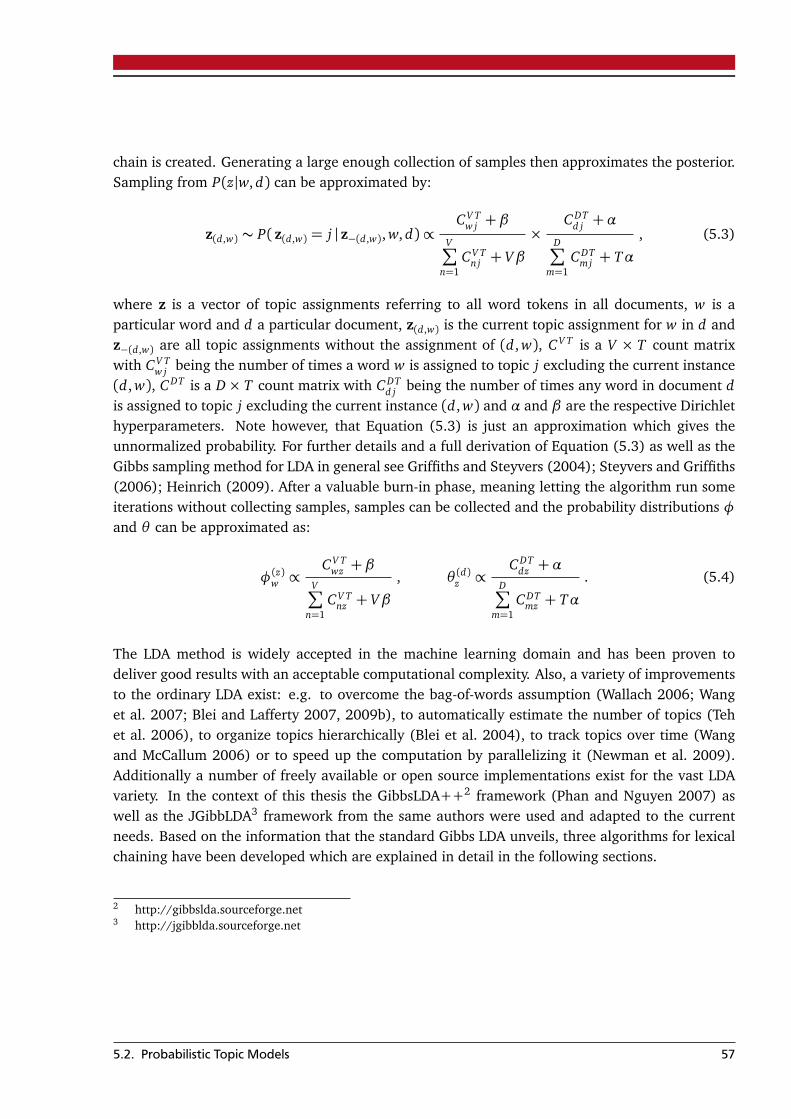
chain is created. Generating a large enough collection of samples then approximates the posterior.Sampling from P(z|w, d) can be approximated by:
z(d,w) ∼ P(z(d,w) = j |z−(d,w), w, d)∝CV T
w j + βV∑
n=1CV T
nj + Vβ
×C DT
d j +αD∑
m=1C DT
mj + Tα
, (5.3)
where z is a vector of topic assignments referring to all word tokens in all documents, w is aparticular word and d a particular document, z(d,w) is the current topic assignment for w in d andz−(d,w) are all topic assignments without the assignment of (d, w), CV T is a V × T count matrixwith CV T
w j being the number of times a word w is assigned to topic j excluding the current instance(d, w), C DT is a D× T count matrix with C DT
d j being the number of times any word in document dis assigned to topic j excluding the current instance (d, w) and α and β are the respective Dirichlethyperparameters. Note however, that Equation (5.3) is just an approximation which gives theunnormalized probability. For further details and a full derivation of Equation (5.3) as well as theGibbs sampling method for LDA in general see Griffiths and Steyvers (2004); Steyvers and Griffiths(2006); Heinrich (2009). After a valuable burn-in phase, meaning letting the algorithm run someiterations without collecting samples, samples can be collected and the probability distributions φand θ can be approximated as:
φ(z)w ∝CV T
wz + βV∑
n=1CV T
nz + Vβ
, θ (d)z ∝C DT
dz +αD∑
m=1C DT
mz + Tα
. (5.4)
The LDA method is widely accepted in the machine learning domain and has been proven todeliver good results with an acceptable computational complexity. Also, a variety of improvementsto the ordinary LDA exist: e.g. to overcome the bag-of-words assumption (Wallach 2006; Wanget al. 2007; Blei and Lafferty 2007, 2009b), to automatically estimate the number of topics (Tehet al. 2006), to organize topics hierarchically (Blei et al. 2004), to track topics over time (Wangand McCallum 2006) or to speed up the computation by parallelizing it (Newman et al. 2009).Additionally a number of freely available or open source implementations exist for the vast LDAvariety. In the context of this thesis the GibbsLDA++2 framework (Phan and Nguyen 2007) aswell as the JGibbLDA3 framework from the same authors were used and adapted to the currentneeds. Based on the information that the standard Gibbs LDA unveils, three algorithms for lexicalchaining have been developed which are explained in detail in the following sections.
2 http://gibbslda.sourceforge.net3 http://jgibblda.sourceforge.net
5.2. Probabilistic Topic Models 57
5.2.1 LDA Mode Method (LDA-MM)
The LDA-MM approach places all word tokens that share the same topic id into the same chain. Thepoint is now how to decide to which topic a word belongs to. The most straightforward approach isto collect a single sample z ∼ P(z|w, d) and use this assignment for chaining. According to Riedland Biemann (2012), a single sample is accompanied by a strong variance. Thus, they proposetwo other techniques for getting a good topic assignment with less variance. The main idea of bothmethods is to collect a number of samples from P(z|w, d) and then pick that topic id z that wasassigned the most. A first methodology collects each last sample of multiple Markov chains withthe same initialization and a second methodology collects multiple samples during the run of asingle Markov chain. The latter is called the mode method and is also applied here.
More formally, let s(d,w) be the vector of assignments that have been collected for a certain wordw in a certain document d with each s(d,w)
i referring to the i-th sampled topic id for (d, w). Inother words, regarding Equation (5.3) let s(d,w)
i be the z(d,w) in the i-th sampling step. Further letz(d,w) be the topic id that was most assigned to the word w with respect to the samples in s(d,w).Precisely, z(d,w) is defined to be the mode in s(d,w)— in case of multiple modes a random mode ischosen, though this never happened in practice during this thesis either.
z(d,w) =mode (s(d,w)) (5.5)
≈ argmaxj(P(z = j|w, d)) (5.6)
The LDA-MM assigns for every word w which is a candidate lexical item of a certain documentd which is assigned the same topic z(d,w) to the same chain; hence implicitly disambiguating theterms.
Level Two Link Extension
The possibility to create level two links is given by taking the second most occurring topic fora given word if it exceeds a certain threshold. Consider an example: A certain candidate itemwith topic 4 as its most occurring topic is chained together with all other lexical items also withtopic 4 as their most occurring topic. If topic 2 occurred the second most in the sample set forthat word and the relative number of occurrences for that topic exceeds for example a fraction of0.3 then the word is linked to any word where topic 2 occurred most. Here it suffices that onlyone link is created instead of tying the candidate item with all other words with topic 2 becausetopics / lexical chains represent ideas and ideas need to be tied only once. According to this, asecond link from items with topic 4 to items with topic 2 can be omitted.
58 5. Statistical Methods for Lexical Chaining
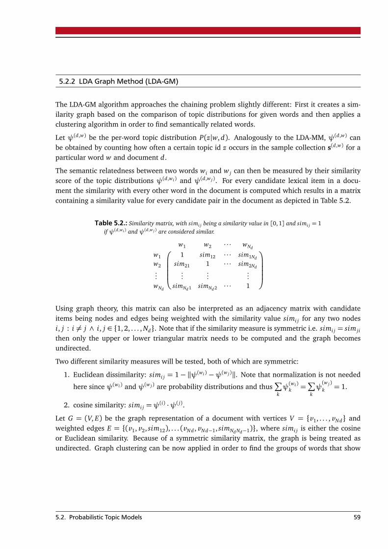
5.2.2 LDA Graph Method (LDA-GM)
The LDA-GM algorithm approaches the chaining problem slightly different: First it creates a sim-ilarity graph based on the comparison of topic distributions for given words and then applies aclustering algorithm in order to find semantically related words.
Let ψ(d,w) be the per-word topic distribution P(z|w, d). Analogously to the LDA-MM, ψ(d,w) canbe obtained by counting how often a certain topic id z occurs in the sample collection s(d,w) for aparticular word w and document d.
The semantic relatedness between two words wi and w j can then be measured by their similarityscore of the topic distributions ψ(d,wi) and ψ(d,w j). For every candidate lexical item in a docu-ment the similarity with every other word in the document is computed which results in a matrixcontaining a similarity value for every candidate pair in the document as depicted in Table 5.2.
Table 5.2.: Similarity matrix, with simi j being a similarity value in [0,1] and simi j = 1if ψ(d,wi ) and ψ(d,w j ) are considered similar.
w1 w2 · · · wNd
w1 1 sim12 · · · sim1Nd
w2 sim21 1 · · · sim2Nd...
......
...wNd
simNd 1 simNd 2 · · · 1
Using graph theory, this matrix can also be interpreted as an adjacency matrix with candidateitems being nodes and edges being weighted with the similarity value simi j for any two nodesi, j : i 6= j ∧ i, j ∈ {1, 2, . . . , Nd}. Note that if the similarity measure is symmetric i.e. simi j = sim ji
then only the upper or lower triangular matrix needs to be computed and the graph becomesundirected.
Two different similarity measures will be tested, both of which are symmetric:
1. Euclidean dissimilarity: simi j = 1− ‖ψ(wi) −ψ(w j)‖. Note that normalization is not needed
here since ψ(wi) and ψ(w j) are probability distributions and thus∑
kψ(wi)k =
∑
kψ(w j)k = 1.
2. cosine similarity: simi j =ψ(i) ·ψ( j).
Let G = (V, E) be the graph representation of a document with vertices V = {v1, . . . , vNd} andweighted edges E = {(v1, v2, sim12), . . . (vNd , vNd−1, simNd Nd−1)}, where simi j is either the cosineor Euclidean similarity. Because of a symmetric similarity matrix, the graph is being treated asundirected. Graph clustering can be now applied in order to find the groups of words that show
5.2. Probabilistic Topic Models 59
a strong level of similarity in their topic distributions. The basic assumption is that each clustergroups together those words that are semantically related. The Chinese Whispers4 (CW) graphclustering algorithm (Biemann 2006) as a special case of Markov Clustering (MCL) algorithms isapplied to find the clusters. A sketch of the algorithm is shown in Listing 5.2 where ci is defined tobe the class label of a vertex v i.
Listing 5.2: The Chinese Whispers algorithm. Vertices with the same class label build thefinal clusters.
1 /* initialize class labels */
2 for i = 1 to |V | do3 ci ← i4 end for5 /* convergence is reached if either
6 * - the algorithm ran a predefined maximum number of iterations, or
7 * - the number of changes is smaller than some predefined threshold or zero */
8 until conv er gence do9 /* update class labels */
10 for each v i ∈ V , randomized−order do11 ci ← predominant_class_in_neighborhood(v i)12 end for13 end for�
The key idea of MCL algorithms is the modeling of a random walker that will most likely not leavea certain group of vertices, i.e. clusters. The property which is thus exploited is called the SmallWorld5 property. The assumption is now that in our scenario a Small World of semantically relatedterms is created. Small World Graphs are sparsely connected with a lot of strongly connectedcomponents. The current graph is densely connected, i.e. each vertex is connected with each othervertex. Hence, in order to create a Small World graph and thus to guarantee good functionality ofChinese Whispers, the weights of the graph’s edges are discretized by the following formula:
simi j :=
¨
0, if simi j < εsim
1, otherwise. (5.7)
By changing the weight of an edge to zero the graph is implicitly pruned since zero-weighted edgesare discarded. Changing the weight to a value of one is optional and not necessarily needed, but
4 An implementation of Chinese Whispers can be found at http://wortschatz.informatik.uni-leipzig.de/~cbiemann/software/CW.html
5 The Small World property for graphs says that a vertex can be reached from any other vertex within a certainnumber of hops (Milgram 1967).
60 5. Statistical Methods for Lexical Chaining
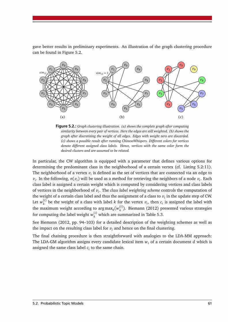
gave better results in preliminary experiments. An illustration of the graph clustering procedurecan be found in Figure 5.2.
v0v1
v2
v3
v4v5
v6
v7
v8
v9sim12
(a)
v0v1
v2
v3
v4v5
v6
v7
v8
v9sim12 = 1
(b)
v0v1
v2
v3
v4
v3
v8
v5
v6
v7
v9
(c)
Figure 5.2.: Graph clustering illustration. (a) shows the complete graph after computingsimilarity between every pair of vertices. Here the edges are still weighted. (b) shows thegraph after discretizing the weight of all edges. Edges with weight zero are discarded.(c) shows a possible result after running ChineseWhispers. Different colors for verticesdenote different assigned class labels. Hence, vertices with the same color form thedesired clusters and are assumed to be related.
In particular, the CW algorithm is equipped with a parameter that defines various options fordetermining the predominant class in the neighborhood of a certain vertex (cf. Listing 5.2:11).The neighborhood of a vertex v i is defined as the set of vertices that are connected via an edge tov i. In the following, n(v i) will be used as a method for retrieving the neighbors of a node v i. Eachclass label is assigned a certain weight which is computed by considering vertices and class labelsof vertices in the neighborhood of v i. The class label weighting scheme controls the computation ofthe weight of a certain class label and thus the assignment of a class to v i in the update step of CW.Let w(i)k be the weight of a class with label k for the vertex v i, then ci is assigned the label with
the maximum weight according to argmaxk(w(i)k ). Biemann (2012) presented various strategies
for computing the label weight w(i)k which are summarized in Table 5.3.
See Biemann (2012, pp. 94–103) for a detailed description of the weighting schemes as well asthe impact on the resulting class label for v i and hence on the final clustering.
The final chaining procedure is then straightforward with analogies to the LDA-MM approach:The LDA-GM algorithm assigns every candidate lexical item wi of a certain document d which isassigned the same class label ci to the same chain.
5.2. Probabilistic Topic Models 61
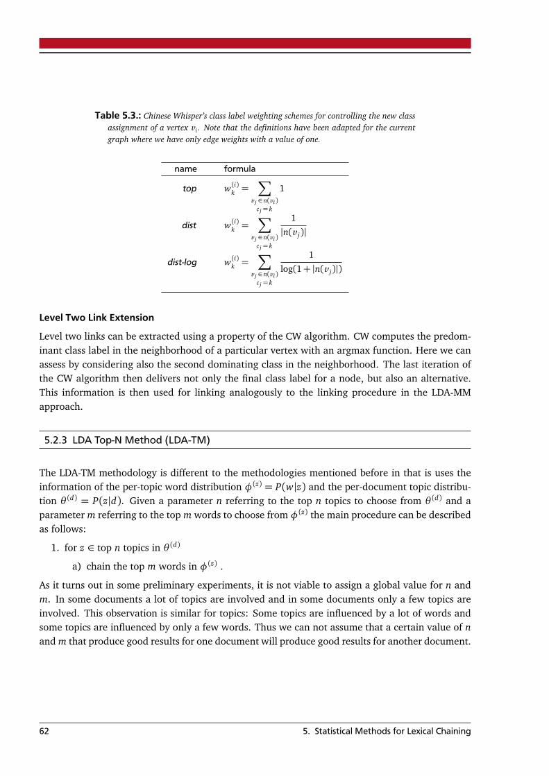
Table 5.3.: Chinese Whisper’s class label weighting schemes for controlling the new classassignment of a vertex v i . Note that the definitions have been adapted for the currentgraph where we have only edge weights with a value of one.
name formula
top w(i)k =∑
v j ∈n(vi)c j = k
1
dist w(i)k =∑
v j ∈n(vi)c j = k
1
|n(v j)|
dist-log w(i)k =∑
v j ∈n(vi)c j = k
1
log(1+ |n(v j)|)
Level Two Link Extension
Level two links can be extracted using a property of the CW algorithm. CW computes the predom-inant class label in the neighborhood of a particular vertex with an argmax function. Here we canassess by considering also the second dominating class in the neighborhood. The last iteration ofthe CW algorithm then delivers not only the final class label for a node, but also an alternative.This information is then used for linking analogously to the linking procedure in the LDA-MMapproach.
5.2.3 LDA Top-N Method (LDA-TM)
The LDA-TM methodology is different to the methodologies mentioned before in that is uses theinformation of the per-topic word distribution φ(z) = P(w|z) and the per-document topic distribu-tion θ (d) = P(z|d). Given a parameter n referring to the top n topics to choose from θ (d) and aparameter m referring to the top m words to choose from φ(z) the main procedure can be describedas follows:
1. for z ∈ top n topics in θ (d)
a) chain the top m words in φ(z) .
As it turns out in some preliminary experiments, it is not viable to assign a global value for n andm. In some documents a lot of topics are involved and in some documents only a few topics areinvolved. This observation is similar for topics: Some topics are influenced by a lot of words andsome topics are influenced by only a few words. Thus we can not assume that a certain value of nand m that produce good results for one document will produce good results for another document.
62 5. Statistical Methods for Lexical Chaining
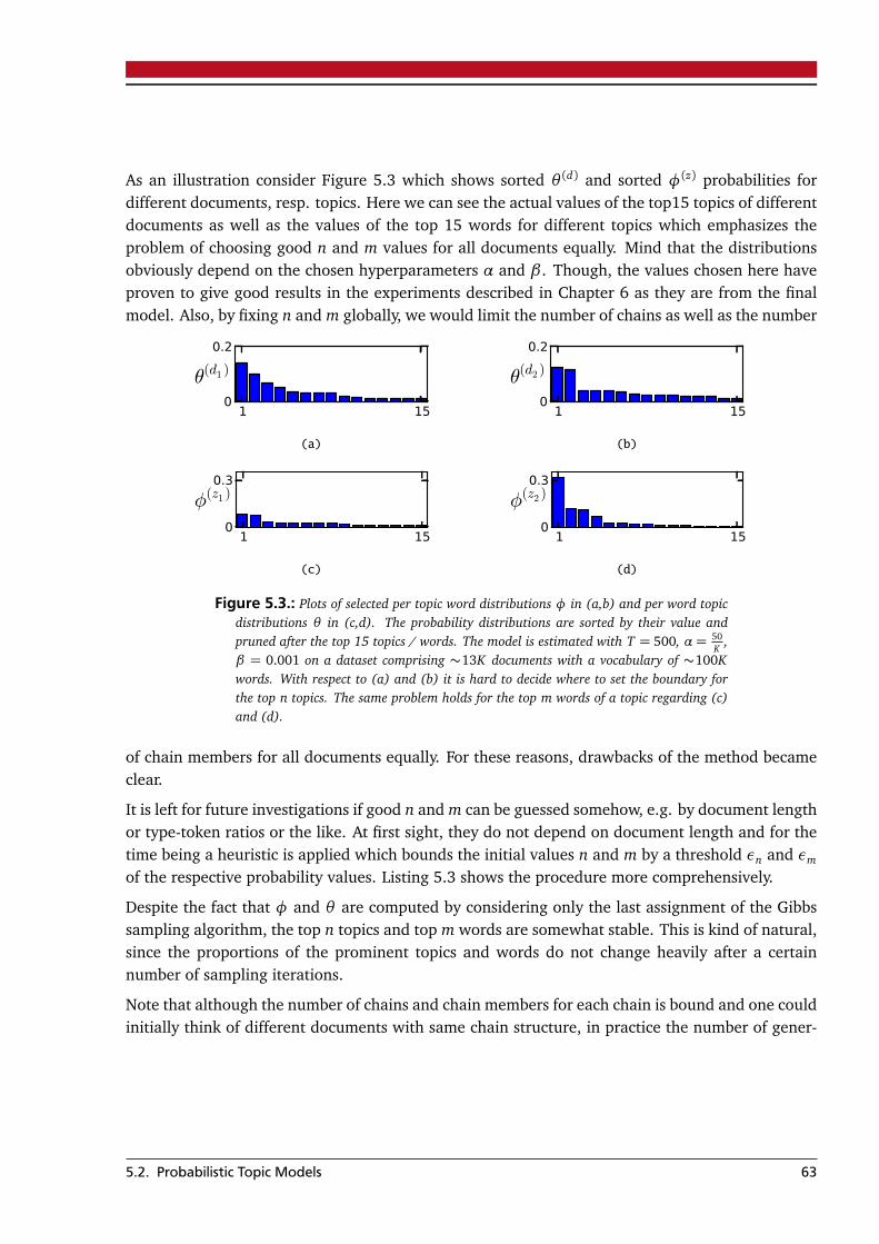
As an illustration consider Figure 5.3 which shows sorted θ (d) and sorted φ(z) probabilities fordifferent documents, resp. topics. Here we can see the actual values of the top15 topics of differentdocuments as well as the values of the top 15 words for different topics which emphasizes theproblem of choosing good n and m values for all documents equally. Mind that the distributionsobviously depend on the chosen hyperparameters α and β . Though, the values chosen here haveproven to give good results in the experiments described in Chapter 6 as they are from the finalmodel. Also, by fixing n and m globally, we would limit the number of chains as well as the number
1 150
0.2
θ(d1 )
(a)
1 150
0.2
θ(d2 )
(b)
1 150
0.3
φ(z1 )
(c)
1 150
0.3
φ(z2 )
(d)
Figure 5.3.: Plots of selected per topic word distributions φ in (a,b) and per word topicdistributions θ in (c,d). The probability distributions are sorted by their value andpruned after the top 15 topics / words. The model is estimated with T = 500, α = 50
K,
β = 0.001 on a dataset comprising ∼13K documents with a vocabulary of ∼100Kwords. With respect to (a) and (b) it is hard to decide where to set the boundary forthe top n topics. The same problem holds for the top m words of a topic regarding (c)and (d).
of chain members for all documents equally. For these reasons, drawbacks of the method becameclear.
It is left for future investigations if good n and m can be guessed somehow, e.g. by document lengthor type-token ratios or the like. At first sight, they do not depend on document length and for thetime being a heuristic is applied which bounds the initial values n and m by a threshold εn and εm
of the respective probability values. Listing 5.3 shows the procedure more comprehensively.
Despite the fact that φ and θ are computed by considering only the last assignment of the Gibbssampling algorithm, the top n topics and top m words are somewhat stable. This is kind of natural,since the proportions of the prominent topics and words do not change heavily after a certainnumber of sampling iterations.
Note that although the number of chains and chain members for each chain is bound and one couldinitially think of different documents with same chain structure, in practice the number of gener-
5.2. Probabilistic Topic Models 63
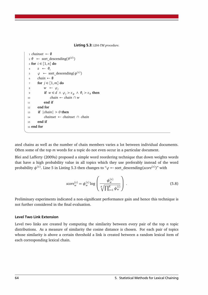
Listing 5.3: LDA-TM procedure.
1 chainset ← ;2 ϑ ← sort_descending(θ (d))3 for i ∈ [1, n] do4 z ← ϑi
5 ϕ ← sort_descending(φ(z))6 chain ← ;7 for j ∈ [1, m] do8 w ← ϕ j
9 if w ∈ d ∧ ϕ j > εφ ∧ ϑi > εθ then10 chain ← chain ∩ w11 end if12 end for13 if |chain| > 0 then14 chainset ← chainset ∩ chain15 end if16 end for�
ated chains as well as the number of chain members varies a lot between individual documents.Often some of the top m words for a topic do not even occur in a particular document.
Blei and Lafferty (2009a) proposed a simple word reordering technique that down weights wordsthat have a high probability value in all topics which they use preferably instead of the wordprobability φ(z). Line 5 in Listing 5.3 then changes to “ϕ← sort_descending(score(z))” with
score(z)w = φ(z)w log
φ(z)w
KÆ
∏Ki=1φ
(i)w
. (5.8)
Preliminary experiments indicated a non-significant performance gain and hence this technique isnot further considered in the final evaluation.
Level Two Link Extension
Level two links are created by computing the similarity between every pair of the top n topicdistributions. As a measure of similarity the cosine distance is chosen. For each pair of topicswhose similarity is above a certain threshold a link is created between a random lexical item ofeach corresponding lexical chain.
64 5. Statistical Methods for Lexical Chaining
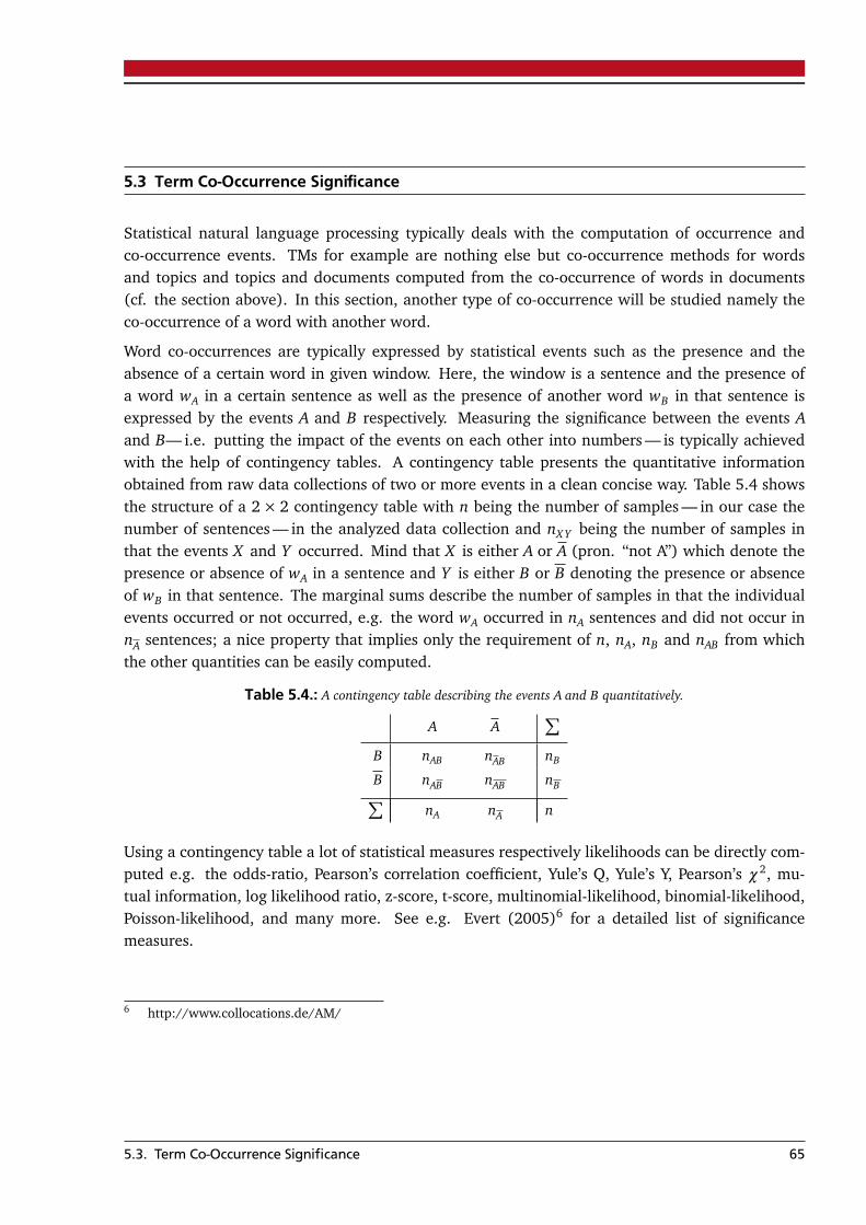
5.3 Term Co-Occurrence Significance
Statistical natural language processing typically deals with the computation of occurrence andco-occurrence events. TMs for example are nothing else but co-occurrence methods for wordsand topics and topics and documents computed from the co-occurrence of words in documents(cf. the section above). In this section, another type of co-occurrence will be studied namely theco-occurrence of a word with another word.
Word co-occurrences are typically expressed by statistical events such as the presence and theabsence of a certain word in given window. Here, the window is a sentence and the presence ofa word wA in a certain sentence as well as the presence of another word wB in that sentence isexpressed by the events A and B respectively. Measuring the significance between the events Aand B— i.e. putting the impact of the events on each other into numbers — is typically achievedwith the help of contingency tables. A contingency table presents the quantitative informationobtained from raw data collections of two or more events in a clean concise way. Table 5.4 showsthe structure of a 2× 2 contingency table with n being the number of samples — in our case thenumber of sentences — in the analyzed data collection and nX Y being the number of samples inthat the events X and Y occurred. Mind that X is either A or A (pron. “not A”) which denote thepresence or absence of wA in a sentence and Y is either B or B denoting the presence or absenceof wB in that sentence. The marginal sums describe the number of samples in that the individualevents occurred or not occurred, e.g. the word wA occurred in nA sentences and did not occur innA sentences; a nice property that implies only the requirement of n, nA, nB and nAB from whichthe other quantities can be easily computed.
Table 5.4.: A contingency table describing the events A and B quantitatively.
A A∑
B nAB nAB nB
B nAB nAB nB∑
nA nA n
Using a contingency table a lot of statistical measures respectively likelihoods can be directly com-puted e.g. the odds-ratio, Pearson’s correlation coefficient, Yule’s Q, Yule’s Y, Pearson’s χ2, mu-tual information, log likelihood ratio, z-score, t-score, multinomial-likelihood, binomial-likelihood,Poisson-likelihood, and many more. See e.g. Evert (2005)6 for a detailed list of significancemeasures.
6 http://www.collocations.de/AM/
5.3. Term Co-Occurrence Significance 65
In this thesis the log likelihood ratio (LLR) (Dunning 1993) is used for testing the significance ofthe events A and B. The LLR as a statistical significance measure is especially used in languagedata because of its adaptability for rare events. Recall that according to Zipf’s Law, words withvery low frequency in everyday use make up the bulk of the vocabulary of a language. Also,these rarely occurring words include many meaning bearing words. Another advantage of theLLR is the asymptotic behavior to the χ2 statistics which allows for the critical values rejectingthe null hypothesis under the χ2 distribution to be valid also for LLR. The results are equivalentlyinterpretable to the results of the χ2 test, i.e. the null hypothesis states that the two events A andB are independent and a higher LLR value rejects the null hypothesis with a higher confidence.The log likelihood ratio can be computed with the help of a contingency table by the followingformula:
LLR = − 2 log(λ)
= 2× [n log(n)− nA log(nA)− nB log(nB) + nAB log(nAB)
+ nAB log(nAB) + nAB log(nAB) + nAB log(nAB)
− nA log(nA)− nB log(nB)]
(5.9)
See Bordag (2007) for details. In practice, the LLR between each pair of words in a given corpusis computed using the TinyCC7 program (Quasthoff et al. 2006) which is able to handle the co-occurrences of a huge number of words.
The lexical chaining procedure is then straightforward with analogies to the LDA-GM procedure.First the LLR scores for a big data collection are computed. When processing a certain documentfor lexical chaining the scores are retrieved for every word pair in that document and inserted intoan adjacency matrix as shown in Table 5.2. Because of the symmetry property of the log likelihoodratio only the upper or lower triangular matrix needs to be created. From this matrix an undirectedgraph as shown in Figure 5.2a can be created and pruned with a specified threshold εl l r continuedby the clustering of the pruned graph with Chinese Whispers. Each word with the same assignedclass label is then assigned to the same chain. This procedure is exactly the same as the “secondpart” of the LDA-GM procedure whereby only the similarity scores between the per-word topicdistributions provided by LDA are exchanged by the LLR scores. This methodology is simply calledthe LLR Graph Method (LLR-GM).
Level Two Link Extension
Level two links are created according to the LDA-GM approach, i.e. by remembering the seconddominant class label in the neighborhood of a certain vertex and using the information for tying
7 http://wortschatz.uni-leipzig.de/~cbiemann/software/TinyCC2.html
66 5. Statistical Methods for Lexical Chaining
the item together with a random item that is assigned this class label (cf. the linking procedure ofLDA-GM in Section 5.2.2).
5.4 Final Notes
All methodologies explained above rely on the statistical analysis of big data collections which iscalled the training set or training documents henceforth. As this, they can be directly applied to anydocument that is in the training set after the analysis.
A plus of the chosen methods is that they can also be applied to new unseen documents that are notin the training set, called test documents henceforth. It is possible to create a trained model basedon the training set and to use this as background information for chaining the test documents.
In order to be adequately applicable, the test documents should be of the same domain as thetraining documents. This is a kind-of obvious restriction since we can not expect the methods towork well when comparing apples and pears.
Though, it may happen that the training documents consist of a slightly different vocabulary asthe test documents. In such cases unknown words cannot be chained adequately. A simple postprocessing step is thus performed after the chaining process of the individual methods which is thechaining of repetitions of unknown words. Recall that repetition is the simplest form of a lexicalcohesive relation.
5.4. Final Notes 67

68 5. Statistical Methods for Lexical Chaining
6 Empirical AnalysisIn this chapter lexical chains produced by the algorithms developed in Chapter 5 are comparedto the manually annotated lexical chains developed in Chapter 4 using the comparison measuredeveloped in Chapter 3.
The lack of manually annotated datasets led to the fact that most of the previous lexical chainingapproaches are evaluated extrinsically by measuring the performance of a particular task that useslexical chain information. This is a valid decision when no data is available but one must not forgetthe reason why no such data exists.
The subjective interpretation of an annotator has an immense impact on the structure of the re-sulting lexical chains. Interpreting a chaining algorithm as an annotator and measuring the qualityof lexical chains extrinsically based on a certain task implies almost always a subjected evaluationto that task. This is perfectly valid since in essence it is the result of the actual task that finallycounts, but one has to be aware that it is actually not the quality of lexical chains in general that ismeasured rather the quality of lexical chains with respect to the particular task is evaluated.
This thesis uses a fraction of the annotated lexical chains developed in Chapter 4 for the intrinsicevaluation of the various statistical algorithms. The other fraction of the annotations is used forthe determination of the algorithm’s parameters; a procedure called model selection. Addition-ally, various trivial baseline algorithms as well as two knowledge-based algorithms are evaluatedwhose results are then compared to the results of the annotators and the results of the developedalgorithms.
6.1 Corpus
The test corpus consists of 100 selected documents of the Salsa/Tiger Corpus which are annotatedduring the work of this thesis as explained in Chapter 4.
The training corpus consists of the Salsa/Tiger documents minus the test documents with inappro-priate texts being heuristically identified and discarded. Precisely, the Salsa/Tiger Corpus consistsof news text from the German newspaper “Frankfurter Rundschau” around 1992. Some of the textsare just short summaries about various happenings which are a kind of news ticker texts. Most ofthese texts share the same structure and are heuristically identified by e.g. the title which is often“Kurznachrichten” or “Nachrichten-Börse” or the like others are signed by multiple press agencies
69
(dpa, rtr, etc.) in different paragraphs which is a clear indicator of false document boundaries.These documents are discarded since they would merely confuse the statistical methods. Addition-ally the training corpus is enriched with news texts from the same newspaper around 1997+ withequal structure. Further, short texts with less than ten candidate lexical items are discarded. Theindividual sizes of the corpora and the sum as the size of the used training corpus are listed inTable 6.1.
Table 6.1.: Size of the training corpus.
corpus #usable documentsSalsa/Tiger 1,211FR 12, 264∑
13,457
6.2 Experimental Setup
In order to qualitatively compare the output of the lexical chaining approaches some trivial baselinealgorithms as well as two non-trivial knowledge based algorithms are considered for comparison.The baseline algorithms are:
All In One: Each candidate item is assigned to the same lexical chain which results in a singlelexical chain per document; no links are created.
Repetitions: Each candidate item and its lexical repetition is assigned a single lexical chain whichresults — in case of no repetitions — in as many lexical chains as there are candidate items;no links are created.
Random: Candidate lexical items are randomly tied together to form sets of lexical chains. Leveltwo links are then created analogously between the resulting lexical chains. Two parameterscontrol the amounts of cohesive ties and level two links in order to build in essence a similarstructure as the manually annotated lexical chains.
S&M GermaNet: Silber and McCoy’s (2002) algorithm (cf. Section 2.2) in combination with Ger-maNet1 (Hamp and Feldweg 1997) is used. The algorithm was implemented in the contextof the work by Jakob (2007) and revised in the context of the work by Schwager (2008).
1 GermaNet is the german equivalent of WORDNET®.
70 6. Empirical Analysis
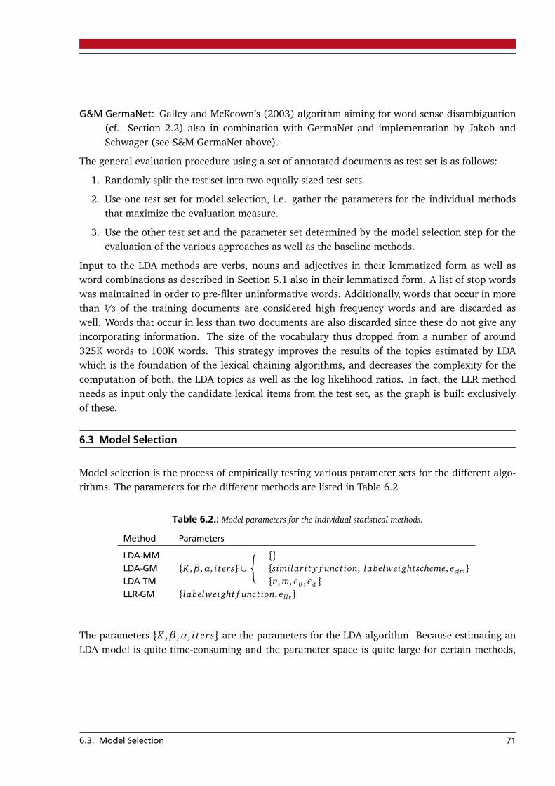
G&M GermaNet: Galley and McKeown’s (2003) algorithm aiming for word sense disambiguation(cf. Section 2.2) also in combination with GermaNet and implementation by Jakob andSchwager (see S&M GermaNet above).
The general evaluation procedure using a set of annotated documents as test set is as follows:
1. Randomly split the test set into two equally sized test sets.
2. Use one test set for model selection, i.e. gather the parameters for the individual methodsthat maximize the evaluation measure.
3. Use the other test set and the parameter set determined by the model selection step for theevaluation of the various approaches as well as the baseline methods.
Input to the LDA methods are verbs, nouns and adjectives in their lemmatized form as well asword combinations as described in Section 5.1 also in their lemmatized form. A list of stop wordswas maintained in order to pre-filter uninformative words. Additionally, words that occur in morethan 1/3 of the training documents are considered high frequency words and are discarded aswell. Words that occur in less than two documents are also discarded since these do not give anyincorporating information. The size of the vocabulary thus dropped from a number of around325K words to 100K words. This strategy improves the results of the topics estimated by LDAwhich is the foundation of the lexical chaining algorithms, and decreases the complexity for thecomputation of both, the LDA topics as well as the log likelihood ratios. In fact, the LLR methodneeds as input only the candidate lexical items from the test set, as the graph is built exclusivelyof these.
6.3 Model Selection
Model selection is the process of empirically testing various parameter sets for the different algo-rithms. The parameters for the different methods are listed in Table 6.2
Table 6.2.: Model parameters for the individual statistical methods.
Method Parameters
LDA-MM{K ,β ,α, i ters} ∪
( {}LDA-GM {similari t y f unct ion, labelweightscheme,εsim}LDA-TM {n, m,εθ ,εφ}LLR-GM {labelweight f unct ion,εl l r}
The parameters {K ,β ,α, i ters} are the parameters for the LDA algorithm. Because estimating anLDA model is quite time-consuming and the parameter space is quite large for certain methods,
6.3. Model Selection 71
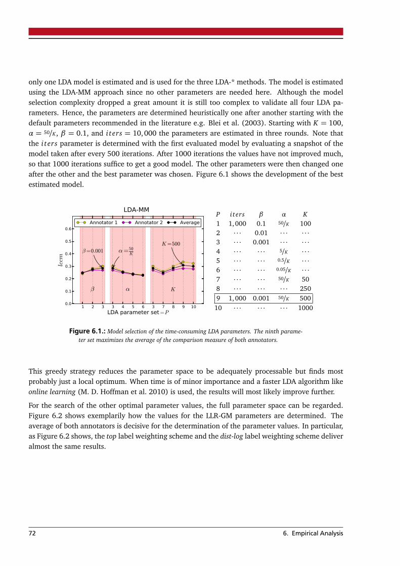
only one LDA model is estimated and is used for the three LDA-* methods. The model is estimatedusing the LDA-MM approach since no other parameters are needed here. Although the modelselection complexity dropped a great amount it is still too complex to validate all four LDA pa-rameters. Hence, the parameters are determined heuristically one after another starting with thedefault parameters recommended in the literature e.g. Blei et al. (2003). Starting with K = 100,α = 50/K, β = 0.1, and i ters = 10,000 the parameters are estimated in three rounds. Note thatthe i ters parameter is determined with the first evaluated model by evaluating a snapshot of themodel taken after every 500 iterations. After 1000 iterations the values have not improved much,so that 1000 iterations suffice to get a good model. The other parameters were then changed oneafter the other and the best parameter was chosen. Figure 6.1 shows the development of the bestestimated model.
1 2 3 3 4 5 6 3 7 8 9 10
LDA parameter set =P
0.0
0.1
0.2
0.3
0.4
0.5
0.6
lccm
β
β=0.001
α
α=50K
K
K=500
Annotator 1 Annotator 2 Average
LDA-MMP iters β α K1 1,000 0.1 50/K 1002 · · · 0.01 · · · · · ·3 · · · 0.001 · · · · · ·4 · · · · · · 5/K · · ·5 · · · · · · 0.5/K · · ·6 · · · · · · 0.05/K · · ·7 · · · · · · 50/K 508 · · · · · · · · · 2509 1, 000 0.001 50/K 500
10 · · · · · · · · · 1000
Figure 6.1.: Model selection of the time-consuming LDA parameters. The ninth parame-ter set maximizes the average of the comparison measure of both annotators.
This greedy strategy reduces the parameter space to be adequately processable but finds mostprobably just a local optimum. When time is of minor importance and a faster LDA algorithm likeonline learning (M. D. Hoffman et al. 2010) is used, the results will most likely improve further.
For the search of the other optimal parameter values, the full parameter space can be regarded.Figure 6.2 shows exemplarily how the values for the LLR-GM parameters are determined. Theaverage of both annotators is decisive for the determination of the parameter values. In particular,as Figure 6.2 shows, the top label weighting scheme and the dist-log label weighting scheme deliveralmost the same results.
72 6. Empirical Analysis
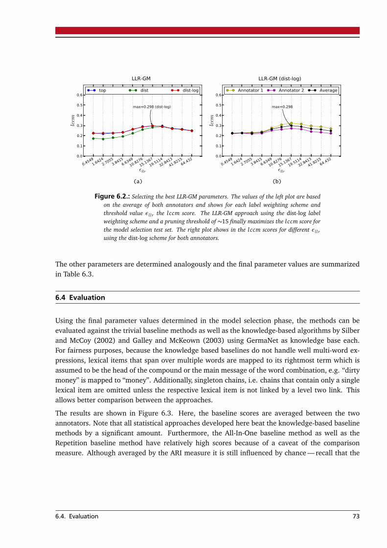
0.45491.6424
2.70553.8415
6.6349
10.8276
15.1367
19.5114
32.8413
41.821564.432
εllr
0.0
0.1
0.2
0.3
0.4
0.5
0.6
lccm
max=0.298 (dist-log)
top dist dist-log
LLR-GM
(a)
0.45491.6424
2.70553.8415
6.6349
10.8276
15.1367
19.5114
32.8413
41.821564.432
εllr
0.0
0.1
0.2
0.3
0.4
0.5
0.6
lccm
max=0.298
Annotator 1 Annotator 2 Average
LLR-GM (dist-log)
(b)
Figure 6.2.: Selecting the best LLR-GM parameters. The values of the left plot are basedon the average of both annotators and shows for each label weighting scheme andthreshold value εl l r the lccm score. The LLR-GM approach using the dist-log labelweighting scheme and a pruning threshold of ∼15 finally maximizes the lccm score forthe model selection test set. The right plot shows in the lccm scores for different εl l r
using the dist-log scheme for both annotators.
The other parameters are determined analogously and the final parameter values are summarizedin Table 6.3.
6.4 Evaluation
Using the final parameter values determined in the model selection phase, the methods can beevaluated against the trivial baseline methods as well as the knowledge-based algorithms by Silberand McCoy (2002) and Galley and McKeown (2003) using GermaNet as knowledge base each.For fairness purposes, because the knowledge based baselines do not handle well multi-word ex-pressions, lexical items that span over multiple words are mapped to its rightmost term which isassumed to be the head of the compound or the main message of the word combination, e.g. “dirtymoney” is mapped to “money”. Additionally, singleton chains, i.e. chains that contain only a singlelexical item are omitted unless the respective lexical item is not linked by a level two link. Thisallows better comparison between the approaches.
The results are shown in Figure 6.3. Here, the baseline scores are averaged between the twoannotators. Note that all statistical approaches developed here beat the knowledge-based baselinemethods by a significant amount. Furthermore, the All-In-One baseline method as well as theRepetition baseline method have relatively high scores because of a caveat of the comparisonmeasure. Although averaged by the ARI measure it is still influenced by chance — recall that the
6.4. Evaluation 73
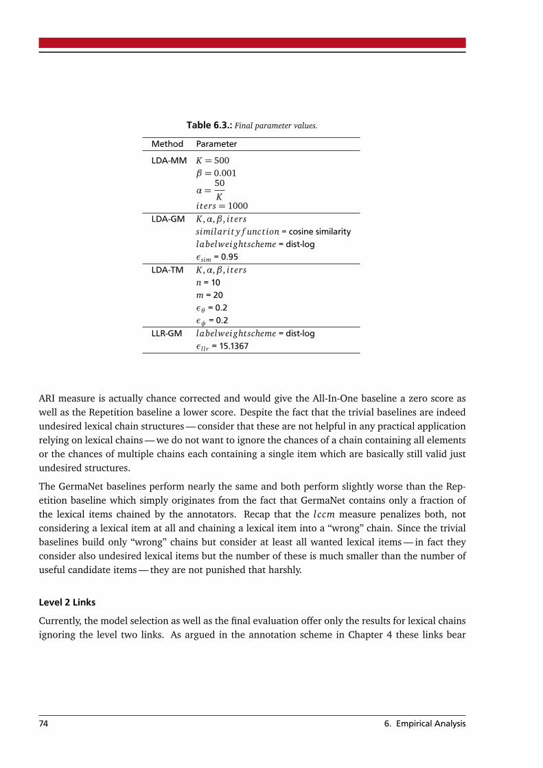
Table 6.3.: Final parameter values.
Method Parameter
LDA-MM K = 500β = 0.001
α=50
Kiters = 1000
LDA-GM K ,α,β , i terssimilari t y f unct ion = cosine similaritylabelweightscheme = dist-logεsim = 0.95
LDA-TM K ,α,β , i tersn = 10m = 20εθ = 0.2εφ = 0.2
LLR-GM labelweightscheme = dist-logεl l r = 15.1367
ARI measure is actually chance corrected and would give the All-In-One baseline a zero score aswell as the Repetition baseline a lower score. Despite the fact that the trivial baselines are indeedundesired lexical chain structures — consider that these are not helpful in any practical applicationrelying on lexical chains — we do not want to ignore the chances of a chain containing all elementsor the chances of multiple chains each containing a single item which are basically still valid justundesired structures.
The GermaNet baselines perform nearly the same and both perform slightly worse than the Rep-etition baseline which simply originates from the fact that GermaNet contains only a fraction ofthe lexical items chained by the annotators. Recap that the lccm measure penalizes both, notconsidering a lexical item at all and chaining a lexical item into a “wrong” chain. Since the trivialbaselines build only “wrong” chains but consider at least all wanted lexical items — in fact theyconsider also undesired lexical items but the number of these is much smaller than the number ofuseful candidate items — they are not punished that harshly.
Level 2 Links
Currently, the model selection as well as the final evaluation offer only the results for lexical chainsignoring the level two links. As argued in the annotation scheme in Chapter 4 these links bear
74 6. Empirical Analysis
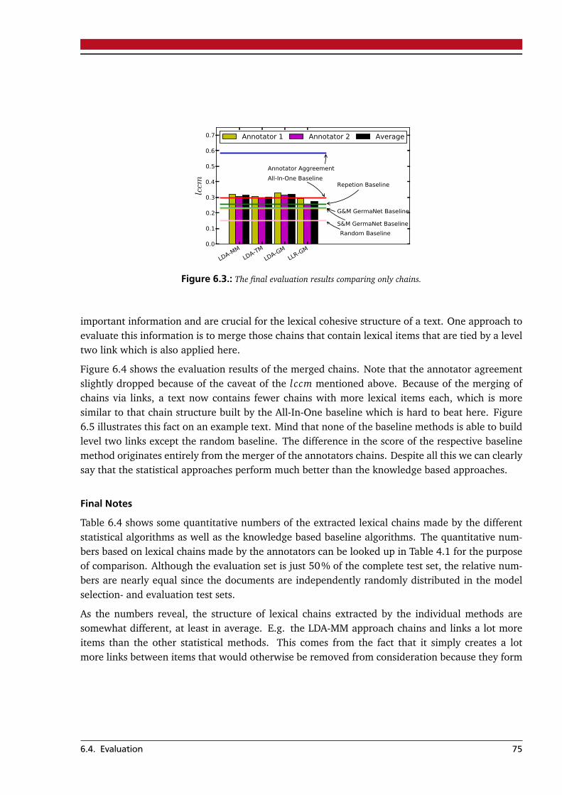
LDA-MM
LDA-TM
LDA-GM
LLR-GM0.0
0.1
0.2
0.3
0.4
0.5
0.6
0.7
lccm
Annotator Aggreement
All-In-One BaselineRepetion Baseline
G&M GermaNet Baseline
S&M GermaNet Baseline
Random Baseline
Annotator 1 Annotator 2 Average
Figure 6.3.: The final evaluation results comparing only chains.
important information and are crucial for the lexical cohesive structure of a text. One approach toevaluate this information is to merge those chains that contain lexical items that are tied by a leveltwo link which is also applied here.
Figure 6.4 shows the evaluation results of the merged chains. Note that the annotator agreementslightly dropped because of the caveat of the lccm mentioned above. Because of the merging ofchains via links, a text now contains fewer chains with more lexical items each, which is moresimilar to that chain structure built by the All-In-One baseline which is hard to beat here. Figure6.5 illustrates this fact on an example text. Mind that none of the baseline methods is able to buildlevel two links except the random baseline. The difference in the score of the respective baselinemethod originates entirely from the merger of the annotators chains. Despite all this we can clearlysay that the statistical approaches perform much better than the knowledge based approaches.
Final Notes
Table 6.4 shows some quantitative numbers of the extracted lexical chains made by the differentstatistical algorithms as well as the knowledge based baseline algorithms. The quantitative num-bers based on lexical chains made by the annotators can be looked up in Table 4.1 for the purposeof comparison. Although the evaluation set is just 50% of the complete test set, the relative num-bers are nearly equal since the documents are independently randomly distributed in the modelselection- and evaluation test sets.
As the numbers reveal, the structure of lexical chains extracted by the individual methods aresomewhat different, at least in average. E.g. the LDA-MM approach chains and links a lot moreitems than the other statistical methods. This comes from the fact that it simply creates a lotmore links between items that would otherwise be removed from consideration because they form
6.4. Evaluation 75
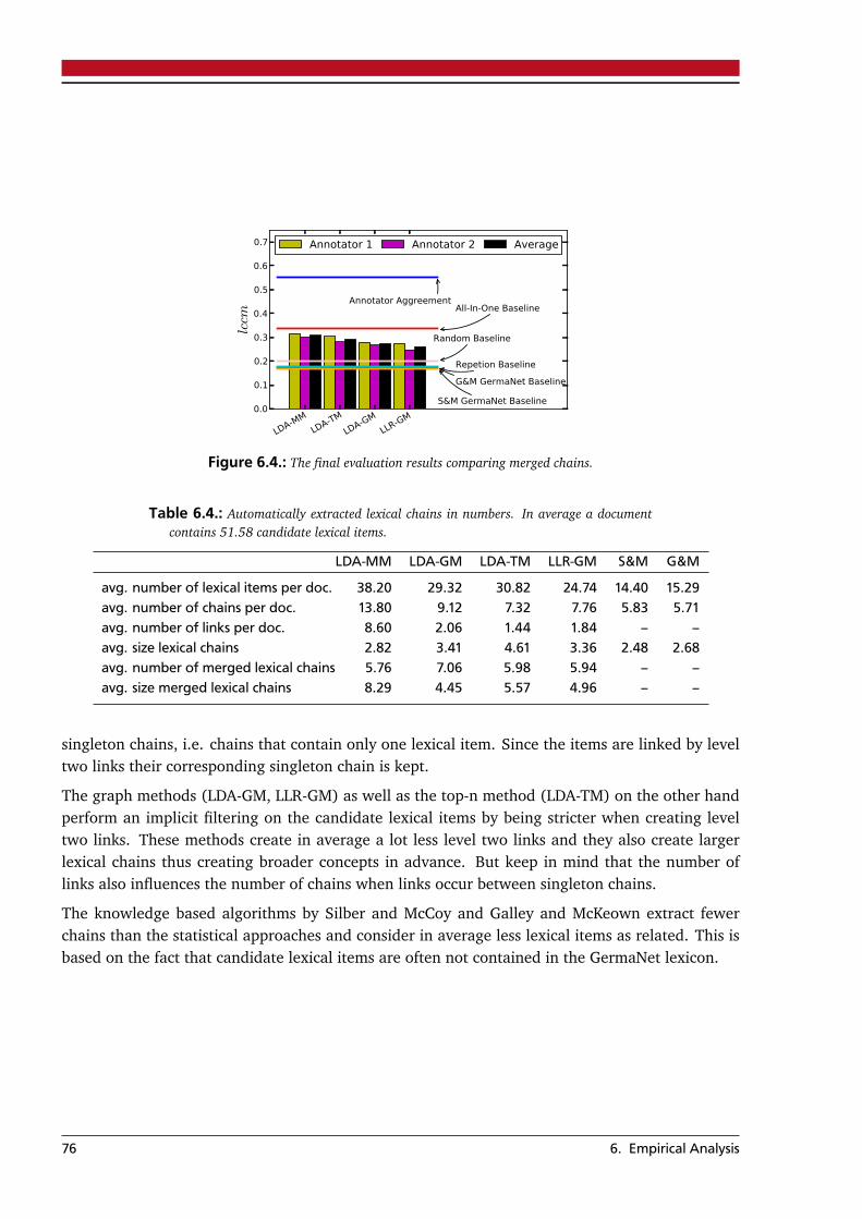
LDA-MM
LDA-TM
LDA-GM
LLR-GM0.0
0.1
0.2
0.3
0.4
0.5
0.6
0.7lccm
Annotator AggreementAll-In-One Baseline
Repetion Baseline
G&M GermaNet Baseline
S&M GermaNet Baseline
Random Baseline
Annotator 1 Annotator 2 Average
Figure 6.4.: The final evaluation results comparing merged chains.
Table 6.4.: Automatically extracted lexical chains in numbers. In average a documentcontains 51.58 candidate lexical items.
LDA-MM LDA-GM LDA-TM LLR-GM S&M G&M
avg. number of lexical items per doc. 38.20 29.32 30.82 24.74 14.40 15.29avg. number of chains per doc. 13.80 9.12 7.32 7.76 5.83 5.71avg. number of links per doc. 8.60 2.06 1.44 1.84 – –avg. size lexical chains 2.82 3.41 4.61 3.36 2.48 2.68avg. number of merged lexical chains 5.76 7.06 5.98 5.94 – –avg. size merged lexical chains 8.29 4.45 5.57 4.96 – –
singleton chains, i.e. chains that contain only one lexical item. Since the items are linked by leveltwo links their corresponding singleton chain is kept.
The graph methods (LDA-GM, LLR-GM) as well as the top-n method (LDA-TM) on the other handperform an implicit filtering on the candidate lexical items by being stricter when creating leveltwo links. These methods create in average a lot less level two links and they also create largerlexical chains thus creating broader concepts in advance. But keep in mind that the number oflinks also influences the number of chains when links occur between singleton chains.
The knowledge based algorithms by Silber and McCoy and Galley and McKeown extract fewerchains than the statistical approaches and consider in average less lexical items as related. This isbased on the fact that candidate lexical items are often not contained in the GermaNet lexicon.
76 6. Empirical Analysis
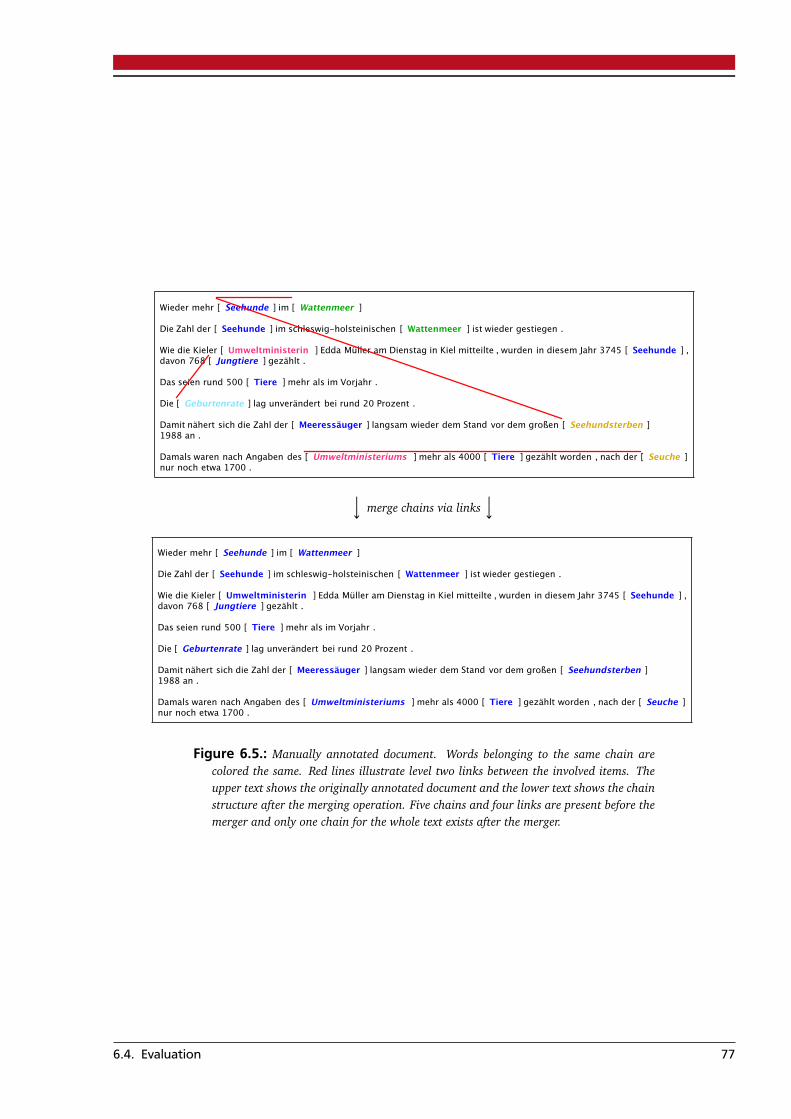
−→ merge chains via links
−→
Figure 6.5.: Manually annotated document. Words belonging to the same chain arecolored the same. Red lines illustrate level two links between the involved items. Theupper text shows the originally annotated document and the lower text shows the chainstructure after the merging operation. Five chains and four links are present before themerger and only one chain for the whole text exists after the merger.
6.4. Evaluation 77

78 6. Empirical Analysis
7 Summary & Conclusion
7.1 Conclusion
Validity of the Hypothesis
The central theme of this thesis is the question if statistical methods can compare with knowledgeresource based methods for the task of lexical chain extraction. In order to test this hypothesis,four newly developed statistical methodologies for lexical chain extraction have been evaluatedagainst some trivial chaining techniques as well as some established knowledge based chainingtechniques with the result that statistical methods significantly outperformed the knowledge basedapproaches. Hence, the outcome of the evaluation confirms the hypothesis.
As argued in the problem statement (cf. Sec. 1.1), the performance of the knowledge based ap-proaches highly depends on the quantity and quality of the content of the utilized knowledgeresource. GermaNet as the knowledge resource used throughout this thesis, though quite com-prehensive, is not comparable in quantity and quality to its English counterpart WordNet. Thus aquantitatively larger and a qualitatively better knowledge resource will most probably improve theperformance of the knowledge based chaining approaches.
Nevertheless, comparable statistical approaches are always preferable over knowledge based ap-proaches as the costs for building a statistical model are much cheaper than the cost for creating areliable knowledge resource.
Limitations & Suggestions
What is a strength of statistical methods is also its major limitation namely the reliance on gooddata collections. This means especially that a corpus of an adequate size — larger is always betterhere — and also of good and uniform quality lets the statistics show its full strength. What isneeded is a hand for the preprocessing of the data as well as a good feeling for the parameters ofthe statistical models especially the LDA methods.
A major problem of the algorithms is the choice of good candidate lexical items. This is also aproblem of knowledge based approaches but of minor interest here since a common approach is toassume all items contained in a knowledge resource to be relevant at all. During this thesis, a sim-ple heuristic is applied for the detection of candidate lexical items. More sophisticated approaches
79
could help here, e.g. the identification of compounds like “small talk” or the like. The statisticalmethods could also gain from prior compound splitting like “bedroom” into “bed” and “room” asthese typically encode multiple topics. This may not be a big problem for the English languagebut applies particularly for the German language where words can be compounded excessivelye.g. the word “Donaudampfschiffahrtsgesellschaftskapitän”1 is a compound of various individualwords. This preprocessing step could improve the statistical reasoning and thus the final statisticalmodel.
Also, in the context of this thesis the algorithms as well as the manual annotations weremostly limited to nouns. This decision was met in order to limit the workload and perform afair evaluation — recall that knowledge based approaches only consider nouns due to structurallimitations — and is not a general limitation. The developed methods are applicable to any kindof words. To include verbs and other parts-of-speech in lexical chaining — just as theoreticallydefined — will most likely enhance the intuitive quality of the lexical chains themselves as wellas most natural language processing tasks that rely on lexical chains, e.g. summarization or textsegmentation or the like.
7.2 Future Divisions & Applications
Carrying out an enhanced annotation project that involves maybe hundreds of annotators couldgive insights into the diverse interpretations of a text by different readers. It would be an interest-ing investigation if the interpretations follow any specific rules. With that many annotators maybean “average interpretation” could be generated which can then be used for further processing.
Another direction is the development of an ultimate lexical chain comparison measure. The heredeveloped lccm is a valid choice but it is still biased by a tradeoff (cf. Sec. 3.4). Fortunately theclustering comparison domain is under heavy development so that better clustering comparisonmeasures may be developed which qualify as lexical chain comparison measure.
Further directions include the development and evaluation of natural language processing appli-cations that rely on statistically extracted lexical chains. Applications that already benefit fromlexical chain extraction are manifold. These need to be adapted to the new methods. An advan-tage is here that next to the lexical chains themselves, also the internal structure of the developedtechniques can be exploited — the similarity graphs of the both graph based approaches (LDA-GMand LLR-GM) for example.
Also, more sophisticated methodologies can be developed that combine statistical and knowledgebased approaches which can then even be extended to supervised approaches that learn from theannotated data.
1 “captain of the Danube Steam Shipping Company”
80 7. Summary & Conclusion
7.3 Summary
Summarizing, in this thesis statistical methods were examined for their applicability for the iden-tification of lexical chains in a cohesive text.
Four algorithms were developed that exploit the statistical foundation of these methods in differ-ent ways in order to extract lexical chain information. The algorithms were built on top of twobranches from statistical natural language processing which are (a) probabilistic topic models, la-tent Dirichlet allocation (LDA) in particular, and (b) statistically significant word co-occurrences.These algorithms have been extended in order to identify not only the cohesive structure of lexicalchains, but also the structure of chain interaction defined by cohesive harmony which is instanti-ated through so-called level two links here.
In order to measure the performance of the approaches an extensive survey of suitable evalua-tion measures was performed. This survey introduced desirable characteristics for the problemof comparing different sets of lexical chains and examines various well-known measures from theclustering domain. Finally a combination of the adjusted Rand index and the normalized basicmerge distance (NBMD) was chosen which best reflects most of the desired characteristics. Thedeveloped measure is simply called the lccm (lexical chain comparison measure) and was used forthe analysis of the interannotator-agreement in the performed annotation project as well as for themodel-selection and final evaluation of the lexical chain extraction algorithms.
An annotation project was realized in order to develop a dataset building a reliable basis for thegeneral evaluation of lexical chains which includes also the level two links. The annotation projectwas kept extensible and can be carried on due to the provision of annotation guidelines and theadaptation of a suited computer-aided annotation framework. During this thesis, two annotatorsannotated around one hundred documents from the German SALSA 2.0 / Tiger 2.1 corpus, therebyenhancing the already comprehensively annotated corpus with information about lexical cohesion.The annotated texts have been analyzed with regard to their inter-annotator agreement using thelccm. The analysis has shown that high inter-annotator agreement is merely possible due to thegeneral problem of subjective interpretations of texts by individual readers.
Using the annotated data and the proposed comparison measure the performance of the devel-oped statistical methods is measured and validated against various trivial lexical chain extractionstrategies as well as some established knowledge based lexical chain extraction algorithms. Op-posing to previous approaches, the evaluation was performed entirely intrinsic which means thatthe extracted lexical chains were compared directly to the manually annotated lexical chains. Thisstrategy is completely new since previous approaches measured the performance of the algorithmssolely on the task the lexical chains were intentionally used for.
7.3. Summary 81
The results of the evaluation have shown that lexical chaining algorithms based on statistical meth-ods significantly outperform lexical chaining algorithms based on knowledge resources. Hence, itcan be said that statistical methods qualify for the extraction of lexical chains in a text and are apreferable choice over knowledge resource based algorithms especially in uncommon domains orresource-scarce languages.
82 7. Summary & Conclusion
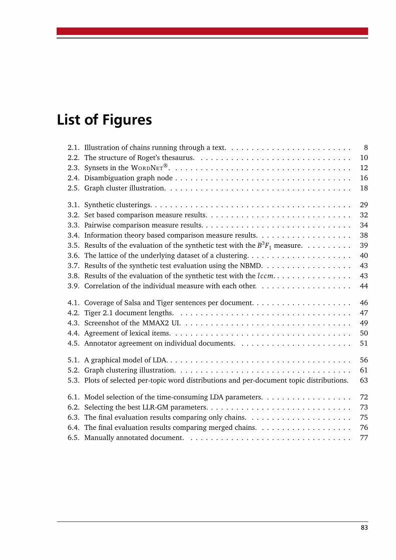
List of Figures2.1. Illustration of chains running through a text. . . . . . . . . . . . . . . . . . . . . . . . . 82.2. The structure of Roget’s thesaurus. . . . . . . . . . . . . . . . . . . . . . . . . . . . . . . 102.3. Synsets in the WORDNET®. . . . . . . . . . . . . . . . . . . . . . . . . . . . . . . . . . . . 122.4. Disambiguation graph node . . . . . . . . . . . . . . . . . . . . . . . . . . . . . . . . . . . 162.5. Graph cluster illustration. . . . . . . . . . . . . . . . . . . . . . . . . . . . . . . . . . . . . 18
3.1. Synthetic clusterings. . . . . . . . . . . . . . . . . . . . . . . . . . . . . . . . . . . . . . . . 293.2. Set based comparison measure results. . . . . . . . . . . . . . . . . . . . . . . . . . . . . 323.3. Pairwise comparison measure results. . . . . . . . . . . . . . . . . . . . . . . . . . . . . . 343.4. Information theory based comparison measure results. . . . . . . . . . . . . . . . . . . 383.5. Results of the evaluation of the synthetic test with the B3F1 measure. . . . . . . . . . 393.6. The lattice of the underlying dataset of a clustering. . . . . . . . . . . . . . . . . . . . . 403.7. Results of the synthetic test evaluation using the NBMD. . . . . . . . . . . . . . . . . . 433.8. Results of the evaluation of the synthetic test with the lccm. . . . . . . . . . . . . . . . 433.9. Correlation of the individual measure with each other. . . . . . . . . . . . . . . . . . . 44
4.1. Coverage of Salsa and Tiger sentences per document. . . . . . . . . . . . . . . . . . . . 464.2. Tiger 2.1 document lengths. . . . . . . . . . . . . . . . . . . . . . . . . . . . . . . . . . . 474.3. Screenshot of the MMAX2 UI. . . . . . . . . . . . . . . . . . . . . . . . . . . . . . . . . . 494.4. Agreement of lexical items. . . . . . . . . . . . . . . . . . . . . . . . . . . . . . . . . . . . 504.5. Annotator agreement on individual documents. . . . . . . . . . . . . . . . . . . . . . . 51
5.1. A graphical model of LDA. . . . . . . . . . . . . . . . . . . . . . . . . . . . . . . . . . . . . 565.2. Graph clustering illustration. . . . . . . . . . . . . . . . . . . . . . . . . . . . . . . . . . . 615.3. Plots of selected per-topic word distributions and per-document topic distributions. 63
6.1. Model selection of the time-consuming LDA parameters. . . . . . . . . . . . . . . . . . 726.2. Selecting the best LLR-GM parameters. . . . . . . . . . . . . . . . . . . . . . . . . . . . . 736.3. The final evaluation results comparing only chains. . . . . . . . . . . . . . . . . . . . . 756.4. The final evaluation results comparing merged chains. . . . . . . . . . . . . . . . . . . 766.5. Manually annotated document. . . . . . . . . . . . . . . . . . . . . . . . . . . . . . . . . 77
83

84 List of Figures
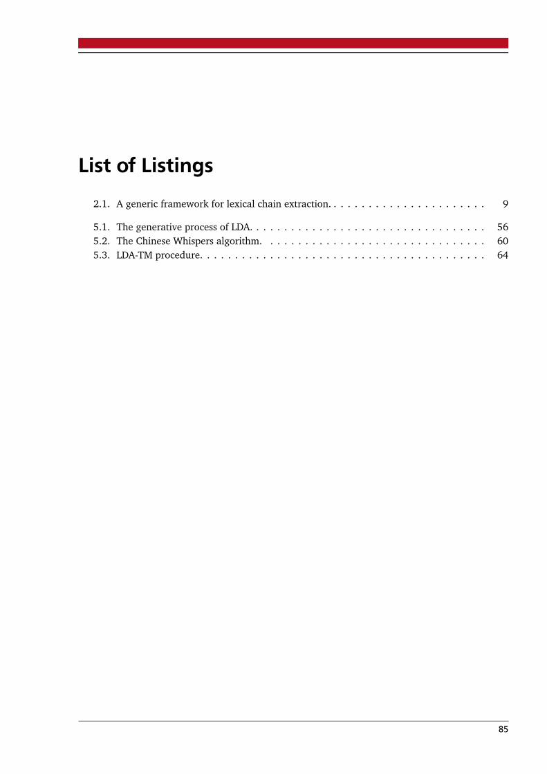
List of Listings2.1. A generic framework for lexical chain extraction. . . . . . . . . . . . . . . . . . . . . . . 9
5.1. The generative process of LDA. . . . . . . . . . . . . . . . . . . . . . . . . . . . . . . . . . 565.2. The Chinese Whispers algorithm. . . . . . . . . . . . . . . . . . . . . . . . . . . . . . . . 605.3. LDA-TM procedure. . . . . . . . . . . . . . . . . . . . . . . . . . . . . . . . . . . . . . . . . 64
85

86 List of Listings
List of Tables
2.1. List of WORDNET® relations. . . . . . . . . . . . . . . . . . . . . . . . . . . . . . . . . . . 122.2. Silber and McCoy’s (2002) lexical relation factors. . . . . . . . . . . . . . . . . . . . . . 162.3. Galley and McKeown’s (2002) lexical relation factors. . . . . . . . . . . . . . . . . . . . 17
4.1. Manually annotated lexical chains in numbers. . . . . . . . . . . . . . . . . . . . . . . . 50
5.1. LDA Terminology. . . . . . . . . . . . . . . . . . . . . . . . . . . . . . . . . . . . . . . . . . 555.2. Similarity matrix. . . . . . . . . . . . . . . . . . . . . . . . . . . . . . . . . . . . . . . . . . 595.3. Chinese Whisper’s class label weighting schemes. . . . . . . . . . . . . . . . . . . . . . 625.4. A contingency table describing the events A and B quantitatively. . . . . . . . . . . . . 65
6.1. Size of the training corpus. . . . . . . . . . . . . . . . . . . . . . . . . . . . . . . . . . . . 706.2. Model parameters for the individual statistical methods. . . . . . . . . . . . . . . . . . 716.3. Final parameter values. . . . . . . . . . . . . . . . . . . . . . . . . . . . . . . . . . . . . . 746.4. Automatically extracted lexical chains in numbers. . . . . . . . . . . . . . . . . . . . . . 76
87

88 List of Tables
BibliographyAjmera, J., Bourlard, H., and Lapidot, I. 2002. Unknown-Multiple Speaker clustering using HMM.
In Proceedings of the international conference of spoken language processing. ICSLP ’02. Denver,Colorado, USA.
Amigó, E., Gonzalo, J., Artiles, J., and Verdejo, F. 2009. A comparison of extrinsic clusteringevaluation metrics based on formal constraints. Information Retrieval 12 (4): 461–486.
Bagga, A. and Baldwin, B. 1998. Algorithms for Scoring Coreference Chains. In Proceedings of thelinguistic coreference workshop at the first international conference on language resources andevaluation, 563–566. LREC ’98. Granada, Spain.
Baker, C. F., Fillmore, C. J., and Lowe, J. B. 1998. The Berkeley FrameNet Project. In COLING ’98:Proceedings of the 17th International Conference on Computational Linguistics, 86–90. Vol. 1.Montreal, Quebec, Canada.
Barzilay, R. 1997. Lexical Chains for Summarization. Master’s thesis, Ben-Gurion University of theNegev.
Barzilay, R. and Elhadad, M. 1997. Using Lexical Chains for Text Summarization. In Proceedingsof the ACL workshop on intelligent scalable text summarization, 10–17. Madrid, Spain.
Benjelloun, O., Garcia-Molina, H., Menestrina, D., Su, Q., Whang, S., and Widom, J. 2009. Swoosh:a generic approach to entity resolution. The VLDB Journal 18:255–276.
Biemann, C. 2006. Chinese Whispers – an Efficient Graph Clustering Algorithm and its Applicationto Natural Language Processing. In Proceedings of textgraphs: the second workshop on graphbased methods for natural language processing, 73–80. New York City, USA.
———. 2012. Structure Discovery in Natural Language. Theory and Applications of Natural Lan-guage Processing. Springer Berlin / Heidelberg.
Blei, D. M. 2012. Probabilistic topic models. Communications of the ACM 55 (4): 77–84.
Blei, D. M. and Lafferty, J. D. 2007. A correlated topic model of science. The Annals of AppliedStatistics 1 (1): 17–35.
89
Blei, D. M. and Lafferty, J. D. 2009a. Topic Models. In Text mining: classification, clustering, andapplications, ed. A. Srivastava and M. Sahami. Data Mining and Knowledge Discovery Series.Boca Raton, Florida, USA: Chapman / Hall/CRC.
———. 2009 b. Visualizing Topics with Multi-Word Expressions. ArXiv e-prints, no.arXiv:0907.1013v1.
Blei, D. M., Ng, A. Y., and Jordan, M. I. 2003. Latent Dirichlet Allocation. Journal of MachineLearning Research 3:993–1022.
Blei, D. M., Griffiths, T. L., Jordan, M. I., and Tenenbaum, J. B. 2004. Hierarchical Topic Models andthe Nested Chinese Restaurant Process. In Advances in Neural Information Processing Systems16, ed. S. B. Thrun S. Saul L.K. Cambridge, Massachusetts, USA: The MIT Press.
Bordag, S. 2007. Elements of Knowledge-free and Unsupervised Lexical Acquisition. PhD diss.,Universität Leipzig.
Boyd-Graber, J., Blei, D. M., and Zhu, X. 2007. A Topic Model for Word Sense Disambiguation.In Proceedings of the 2007 joint conference on empirical methods in natural language processingand computational natural language learning (EMNLP-CoNLL), 1024–1033. Prague, CzechRepublic.
Brants, S., Dipper, S., Hansen, S., Lezius, W., and Smith, G. 2002. TIGER Treebank. In Proceedingsof the workshop on treebanks and linguistic theories (TLT02). Sozopol, Bulgaria.
Bronstein, I. N., Semendjajew, K. A., Musiol, G., and Mühlig, H. 2005. Taschenbuch der Mathematik.6th ed. Frankfurt a.M., Germany: Verlag Harri Deutsch.
Burchardt, A., Erk, K., Frank, A., Kowalski, A., Padó, S., and Pinkal, M. 2006. The SALSA Corpus: aGerman corpus resource for lexical semantics. In Proceedings of the 5th international conferenceon language resources and evaluation (LREC-2006). Genoa, Italy.
Cai, J., Lee, W. S., and Teh, Y. W. 2007. Improving Word Sense Disambiguation Using TopicFeatures. In Proceedings of the 2007 joint conference on empirical methods in natural languageprocessing and computational natural language learning (EMNLP-CoNLL), 1015–1023. Prague,Czech Republic.
Carthy, J. 2004. Lexical Chains versus Keywords for Topic Tracking. In Computational linguisticsand intelligent text processing, ed. A. Gelbukh, 507–510. Vol. 2945. Lecture Notes in ComputerScience. Berlin / Heidelberg: Springer.
Cover, T. M. and Thomas, J. A. 1991. Elements of information theory. Hoboken, New Jersey, USA:Wiley.
90 Bibliography
Cramer, I., Finthammer, M., Kurek, A., Sowa, L., Wachtling, M., and Claas, T. 2008. Experimentson Lexical Chaining for German Corpora: Annotation, Extraction, and Application. Journal forLanguage Technology and Computational Linguistics (JLCL) 23 (2): 34–48.
Deerwester, S., Dumais, S. T., Furnas, G. W., Landauer, T. K., and Harshman, R. 1990. Indexingby latent semantic analysis. Journal of the American Society for Information Science 41 (6):391–407.
Dinu, G. and Lapata, M. 2010. Topic Models for Meaning Similarity in Context. In COLING ’10:Proceedings of the 23rd International Conference on Computational Linguistics: Posters, 250–258. Beijing, China.
Dunning, T. 1993. Accurate Methods for the Statistics of Surprise and Coincidence. ComputationalLinguistics 19 (1): 61–74.
Ercan, G. and Cicekli, I. 2007. Using lexical chains for keyword extraction. Inf. Process. Manage.43 (6): 1705–1714.
Evert, S. 2005. The Statistics of Word Cooccurrences: Word Pairs and Collocations. PhD diss.,Universität Stuttgart.
Fellbaum, C. 1998. WordNet: An Electronic Lexical Database. Language, Speech, and Communica-tion. Cambridge, Massachusetts, USA: The MIT Press.
Gale, W. A., Church, K. W., and Yarowsky, D. 1992. One Sense Per Discourse. In Proceedings of theworkshop on speech and natural language, 233–237. Harriman, New York, USA.
Galley, M. and McKeown, K. 2003. Improving word sense disambiguation in lexical chaining. InIJCAI’03: proceedings of the 18th international joint conference on artificial intelligence, 1486–1488. Acapulco, Mexico.
Girolami, M. and Kabán, A. 2003. On an Equivalence between PLSI and LDA. In SIGIR 2003: Pro-ceedings of the 26th Annual International ACM SIGIR Conference on Research and Developmentin Information Retrieval, 433–434. Toronto, Canada.
Gong, Y. and Liu, X. 2001. Generic Text Summarization Using Relevance Measure and Latent Se-mantic Analysis. In SIGIR 2001: Proceedings of the 24th Annual International ACM SIGIR Con-ference on Research and Development in Information Retrieval, 19–25. New Orleans, Louisiana,USA.
Green, S. J. 1996. Using Lexical Chains to Build Hypertext Links in Newspaper Articles. In AAAI-96workshop on internet-based information systems, 115–141. Portland, Oregon, USA.
Griffiths, T. L. and Steyvers, M. 2004. Finding scientific topics. Proceedings of the National Academyof Sciences of the United States of America 101 (Suppl 1): 5228–5235.
Bibliography 91
Al-Halimi, R. and Kazman, R. 1998. Temporal Indexing through Lexical Chaining. In WordNet: anelectronic lexical database, ed. C. Fellbaum, 333–351. Language, Speech, and Communication.Cambridge, Massachusetts, USA: The MIT Press.
Halliday, M. A. K. and Hasan, R. 1976. Cohesion in English. English language series. London:Longman.
Hamp, B. and Feldweg, H. 1997. GermaNet - a Lexical-Semantic Net for German. In Proceedingsof the ACL/EACL-97 workshop automatic information extraction and building of lexical semanticresources for NLP applications. Madrid, Spain.
Hasan, R. 1984. Coherence and Cohesive Harmony. In Understanding Reading Comprehension, ed.J. Flood, 181–220. Cognition, Language, and the Structure of Prose. Newark, Delaware, USA:International Reading Association.
Hearst, M. A. 1994. Multi-paragraph segmentation of expository text. In Proceedings of the 32ndannual meeting on association for computational linguistics, 9–16. ACL ’94. Las Cruces, NewMexico, USA.
Heinrich, G. 2009. Parameter estimation for text analysis v2.9. Technical report. Darmstadt,Germany: Fraunhofer IGD.
Hennig, L. 2009. Topic-based multi-document summarization with probabilistic latent seman-tic analysis. In Proceedings of the international conference RANLP-2009, 144–149. Borovets,Bulgaria.
Hirst, G. and St-Onge, D. 1998. Lexical Chains as representation of context for the detectionand correction malapropisms. In WordNet: An Electronic Lexical Database, ed. C. Fellbaum,305–332. Language, Speech, and Communication. Cambridge, Massachusetts, USA: The MITPress.
Hoey, M. 1991. Patterns of Lexis in Text. Describing English Language. Oxford, UK: OxfordUniversity Press.
Hoffman, M. D., Blei, D. M., and Bach, F. R. 2010. Online Learning for Latent Dirichlet Allocation.In Advances in Neural Information Processing Systems 23, ed. J. Lafferty, C. K. I. Williams, J.Shawe-Taylor, R. Zemel, and A. Culotta, 856–864. Cambridge, Massachusetts, USA: The MITPress.
Hoffman, M., Blei, D. M., Wang, C., and Paisley, J. 2012. Stochastic Variational Inference. ArXive-prints, no. arXiv:1206.7051v1.
Hofmann, T. 1999a. Probabilistic Latent Semantic Analysis. In Proceedings of the Fifteenth Confer-ence on Uncertainty in Artificial Intelligence, 289–296. UAI ’99. Stockholm, Sweden.
92 Bibliography
———. 1999 b. Probabilistic Latent Semantic Indexing. In SIGIR ’99: Proceedings of the 22nd An-nual International ACM SIGIR Conference on Research and Development in Information Retrieval,50–57. Berkeley, California, USA.
Hollingsworth, W. and Teufel, S. 2005. Human annotation of lexical chains: Coverage and agree-ment measures. In Proceedings of the Workshop ELECTRA: Methodologies and Evaluation ofLexical Cohesion Techniques in Real-world Applications. In Association with SIGIR ’05. Sal-vador, Brazil.
Hubert, L. and Arabie, P. 1985. Comparing partitions. Journal of Classification 2 (1): 193–218.
Jakob, N. 2007. Developing a generic interface for semantic networks. Diploma thesis, TechnischeUniversität Darmstadt.
Jarmasz, M. 2003. Roget’s thesaurus as a lexical resource for natural language processing. Master’sthesis, University of Ottawa.
Lin, C.-Y. and Hovy, E. 2000. The Automated Acquisition of Topic Signatures for Text Summariza-tion. In COLING ’00: Proceedings of the 18th Conference on Computational Linguistics, 495–501.Vol. 1. Saarbrücken, Germany.
Manning, C., Raghavan, P., and Schütze, H. 2008. An Introduction to Information Retrieval. Cam-bridge, UK: Cambridge University Press.
Manning, C. and Schütze, H. 1999. Foundations of Statistical Natural Language Processing. Cam-bridge, Massachusetts, USA: The MIT Press.
Marathe, M. and Hirst, G. 2010. Lexical Chains Using Distributional Measures of Concept D. InProceedings of the 11th International Conference on Computational Linguistics and IntelligentText Processing, 291–302. CICLing’10. Iasi, Romania.
Medelyan, O. 2007. Computing lexical chains with graph clustering. In Proceedings of the 45thAnnual Meeting of the ACL: Student Research Workshop, 85–90. ACL ’07. Prague, CzechRepublic.
Meila, M. 2003. Comparing clusterings by the variation of information. In Proceedings of the 16thAnnual Conference of Computational Learning Theory (COLT). Washington, D.C., USA.
———. 2005. Comparing clusterings: an axiomatic view. In Proceedings of the 22nd InternationalConference on Machine Learning, 577–584. ICML ’05. Bonn, Germany.
———. 2007. Comparing clusterings—an information based distance. Journal of MultivariateAnalysis 98 (5): 873–895.
Bibliography 93
Menestrina, D., Whang, S. E., and Garcia-Molina, H. 2010. Evaluating entity resolution results.Proceedings of the VLDB Endowment 3 (1): 208–219.
Milgram, S. 1967. The Small World Problem. Psychology Today 67 (1): 61–67.
Misra, H., Yvon, F., Jose, J., and Cappé, O. 2009. Text Segmentation via Topic Modeling: AnAnalytical Study. In Proceedings of the 18th ACM Conference on Information and KnowledgeManagement, 1553–1556. CIKM 2009. Hong Kong, China.
Moldovan, D. and Novischi, A. 2002. Lexical chains for question answering. In COLING ’02:Proceedings of the 19th International Conference on Computational Linguistics, 1–7. Taipei,Taiwan.
Morris, J. 2010. Individual Differences in the Interpretation of Text: Implications for InformationScience. Journal of the American Society for Information Science and Technology (JASIST) 61(1): 141–149.
Morris, J. and Hirst, G. 1991. Lexical cohesion computed by thesaural relations as an indicator ofthe structure of text. Computational Linguistics 17:21–48.
———. 2004. The Subjectivity of Lexical Cohesion in Text. In Proceedings of the AAAI spring sym-posium on exploring attitude and affect in text: theories and applications. Palo Alto, California,USA.
Müller, C. and Strube, M. 2006. Multi-level annotation of linguistic data with MMAX2. In Corpustechnology and language pedagogy: new resources, new tools, new methods, ed. S. Braun, K.Kohn, and J. Mukherjee, 197–214. Frankfurt a.M., Germany: Peter Lang.
Nelken, R. and Shieber, S. M. 2007. Lexical Chaining and Word-Sense-Disambiguation. TR-06-07.Technical Report. Cambridge, Massachusetts, USA: Harvard University.
Newman, D., Asuncion, A., Smyth, P., and Welling, M. 2009. Distributed Algorithms for TopicModels. Journal of Machine Learning Research 10:1801–1828.
Okumura, M. and Honda, T. 1994. Word sense disambiguation and text segmentation based on lex-ical cohesion. In COLING ’94: Proceedings of the 15th Conference on Computational Linguistics,755–761. Vol. 2. Kyoto, Japan.
Phan, X.-H. and Nguyen, C.-T. 2007. GibbsLDA++: A C/C++ implementation of latent Dirichletallocation (LDA). http://gibbslda.sourceforge.net.
Quasthoff, U., Richter, M., and Biemann, C. 2006. Corpus Portal for Search in Monolingual Cor-pora. In Proceedings of the 5th international conference on language resources and evaluation(LREC-2006). Genoa, Italy.
94 Bibliography
Rand, W. M. 1971. Objective criteria for the evaluation of clustering methods. Journal of theAmerican Statistical Association 66 (336): 846–850.
Reeve, L., Han, H., and Brooks, A. D. 2006. Biochain: Lexical Chaining Methods for BiomedicalText Summarization. In Proceedings of the 2006 ACM symposium on applied computing (SAC2006), 180–184. Dijon, France.
Reichart, R. and Rappoport, A. 2009. The NVI clustering evaluation measure. In Proceedings ofthe Thirteenth Conference on Computational Natural Language Learning, 165–173. CoNLL ’09.Boulder, Colorado, USA.
Riedl, M. and Biemann, C. 2012. Sweeping through the Topic Space: Bad luck? Roll again! InROBUS-UNSUP 2012: Joint Workshop on Unsupervised and Semi-Supervised Learning in NLPheld in conjunction with EACL 2012, 19–27. Avignon, France.
Roget, P. M. 1852. Roget’s thesaurus of english words and phrases. Harlow, UK: Longman GroupLtd.
Rosenberg, A. and Hirschberg, J. 2007. V-measure: a conditional entropy-based external clusterevaluation measure. In Proceedings of the 2007 joint conference on empirical methods in NaturalLanguage Processing and computational natural language learning (EMNLP-CoNLL), 410–420.Prague, Czech Republic.
Schwager, F. 2008. Automatic analysis of lexical cohesion. Diploma thesis, Technische UniversitätDarmstadt.
Silber, H. G. and McCoy, K. F. 2002. Efficiently computed lexical chains as an intermediate repre-sentation for automatic text summarization. Computational Linguistics 28 (4): 487–496.
Stairmand, M. A. 1996. A computational analysis of lexical cohesion with applications in informa-tion retrieval. PhD diss., Center for Computational Linguistics, UMIST.
Stenetorp, P., Pyysalo, S., Topic, G., Ohta, T., Ananiadou, S., and Tsujii, J. 2012. Brat: a Web-basedTool for NLP-Assisted Text Annotation. In Proceedings of the demonstrations session at EACL2012. Avignon, France.
Steyvers, M. and Griffiths, T. L. 2006. Probabilistic topic models. In Latent semantic analysis: a roadto meaning. Ed. T. Landauer, D. Mcnamara, S. Dennis, and W. Kintsch. Laurence Erlbaum.
Stokes, N., Carthy, J., and Smeaton, A. F. 2004. SeLeCT: A Lexical Cohesion Based News StorySegmentation System. AI Communications 17 (1): 3–12.
Strehl, A. 2002. Relationship-based clustering and cluster ensembles for high-dimensional datamining. PhD diss., University of Texas.
Bibliography 95
Strehl, A. and Ghosh, J. 2003. Cluster Ensembles — A Knowledge Reuse Framework for CombiningMultiple Partitions. Journal of Machine Learning Research 3:583–617.
Stührenberg, M., Goecke, D., Diewald, N., Mehler, A., and Cramer, I. 2007. Web-based annotationof anaphoric relations and lexical chains. In Proceedings of the Linguistic Annotation Workshop(the LAW), 140–147. Prague, Czech Republic.
Teh, Y. W., Newman, D., and Welling, M. 2007. A Collapsed Variational Bayesian Inference Algo-rithm for Latent Dirichlet Allocation. In Advances in Neural Information Processing Systems 19,ed. B. Schölkopf, J. Platt, and T. Hoffman, 1353–1360. Cambridge, Massachusetts, USA: TheMIT Press.
Teh, Y. W., Jordan, M. I., Beal, M. J., and Blei, D. M. 2006. Hierarchical Dirichlet Processes. Journalof the American Statistical Association 101 (476): 1566–1581.
Teich, E. and Fankhauser, P. 2005. Exploring Lexical Patterns in Text: Lexical Cohesion Analysiswith WordNet. In Heterogeneity in Focus: Creating and Using Linguistic Databases, 129–145.Vol. 2. Interdisciplinary Studies on Information Structure (ISIS). Potsdam: UniversitätsverlagPotsdam.
Tomokiyo, T. and Hurst, M. 2003. A language Model Approach to Keyphrase Extraction. In Proceed-ings of the ACL 2003 workshop on Multiword expressions: analysis, acquisition and treatment,33–40. Vol. 18. MWE ’03. Sapporo, Japan.
Wallach, H. M. 2006. Topic modeling: beyond bag-of-words. In Proceedings of the 23rd Inter-national Conference on Machine Learning, 977–984. ICML ’06. Pittsburgh, Pennsylvania,USA.
Wang, X. and McCallum, A. 2006. Topics over Time: A Non-Markov Continuous-Time Model ofTopical Trends. In Proceedings of the 12th ACM SIGKDD International Conference on KnowledgeDiscovery and Data Mining, 424–433. KDD 2006. Philadelphia, Pennsylvania, USA.
Wang, X., McCallum, A., and Wei, X. 2007. Topical n-grams: phrase and topic discovery, withan application to information retrieval. In Proceedings of the 2007 Seventh IEEE InternationalConference on Data Mining, 697–702. ICDM ’07. Omaha, Nebraska, USA.
Yang, D. and Powers, D. M. W. 2006. Word Sense Disambiguation using lexical cohesion in thecontext. In Proceedings of the COLING/ACL 2006 main conference poster sessions, 929–936.Sydney, Australia.
96 Bibliography
A Proof: Equality of NMI and Vto show:
V (C , K)≡ N M I(C , K) (A.1)
with
V (C , K) = 2×h× c
h+ c(A.2)
h= 1−H(C |K)H(C)
, c = 1−H(K |C)H(K)
(A.3)
and
N M I(C , K) = 2×I(C , K)
H(C) +H(K)(A.4)
reformulate h and c using the fact that I(C , K) = H(C)−H(C |K) = H(K)−H(K |C):
h= 1−H(C |K)H(C)
=H(C)H(C)
−H(C |K)H(C)
=H(C)−H(C |K)
H(C)
=I(C , K)H(C)
(A.5)
c = 1−H(K |C)H(K)
=H(K)H(K)
−H(K |C)H(K)
=H(K)−H(K |C)
H(K)
=I(C , K)H(K)
(A.6)
97
simplifying h× c:
h× c =I(C , K)H(C)
×I(C , K)H(K)
=I(C , K)2
H(C)H(K)
(A.7)
simplifying h+ c:
h+ c =I(C , K)H(C)
+I(C , K)H(K)
=I(C , K)H(K)H(C)H(K)
+I(C , K)H(C)H(C)H(K)
=I(C , K)(H(K) + I(C , K)H(C)
H(C)H(K)
=I(C , K)[(H(K) +H(C)]
H(C)H(K)
(A.8)
simplifying h×ch+c
using (A.7) and (A.8):
h× c
h+ c=
I(C , K)2
H(C)H(K)I(C , K)[(H(K) +H(C)]
H(C)H(K)
=I(C , K)2
H(C)H(K)�
I(C , K)[H(K) +H(C)]H(C)H(K)
�−1
=I(C , K)2
H(C)H(K)×
H(C)H(K)I(C , K)[(H(K) +H(C)]
=I(C , K)
H(K) +H(C)
(A.9)
substituting (A.9) into (A.2) shows that NMI and V are equal:
V (C , K) = 2×h× c
h+ c
= 2×I(C , K)
H(K) +H(C)
= N M I(C , K)
(A.10)
98 A. Proof: Equality of NMI and V
B Annotation Guidelines
99
— Lexical Chain Annotation Guidelines —
Steffen Remus
v1.0 – September 1, 2012
About the document
Use this document as a schema to identify and annotate lexical chains indocuments of the current Salsa1 2.0 / TiGer2 2.1 Corpus. This documentguides you through common standards and potential pitfalls.
Introduction to lexical chains
When reading a text, whether short or long, the text is intelligible becauseof its structure. Each text is designed to transport a message, and a reason-able structure is the essential means for this. Lexical chains visualize thisstructure by connecting words or phrases in the text that are semanticallyrelated. These words or phrases are called lexical items and each item con-tributes to a specific meaning of a lexical chain. Consider the given exampletext below and some extracted lexical chains:
COFFEE QUOTA TALKS CONTINUE BUT NO AGREEMENT YET
LONDON, March 2 - Coffee quota talks at theInternational Coffee Organization council meeting herecontinued this afternoon, but producers and consumersstill had not reached common ground on the key issue ofhow to estimate export quotas, delegates said.
The 54 member contact group was examining a Colombianproposal to resume quotas April 1 under the ad hocsystem used historically, with a pledge to meet againin September to discuss how quotas would be worked out inthe future, they said.
1. SALSA – The Saarbrücken Lexical Semantics Acquisition Project, “see A. Burchardtet al. 2006. The SALSA Corpus: a German corpus resource for lexical semantics. InProceedings of the 5th international conference on language resources and evaluation(LREC-2006). Genoa, Italy”.
2. TiGer – TiGer Treebank (Version 2.1), see “S. Brants et al. 2002. TIGER Tree-bank. In Proceedings of the workshop on treebanks and linguistic theories (TLT02).Sozopol, Bulgaria”.
1
1. { COFFEE QUOTA TALKS, Coffee quota talks, Coffee Organi-zation council meeting, quotas, quotas, quotas }2. { CONTINUE, continued, resume }3. { AGREEMENT, reached common ground, pledge, discuss }4. { producers, consumers }
Related terms are underlined with the same color, which build up the chains1-4.
Although the example is incomplete yet (meaning there are more chains inthe text), the central theme of the text (by just looking at the chains) clearlycan be identified.
This technique can be utilized in many applications, and the main goal is toautomatically identify these chains with the help of computer systems. Inorder to evaluate these systems, i.e. to say how good or bad they did thejob, we need examples annotated by humans and compare them with thosemade by the system.
Short Description
• Lexical items are the basic elements of the chains occurring in the texts.
• Candidates for lexical items are words or phrases bearing some mean-ing.
• Lexical items describing the same concept or relating to the same topicform a so-called dense chain.
• Within dense chains each item must be of the same topic as every otheritem in the chain.
• Each lexical item must solely exist in exactly one chain.
• Chains consisting of only a single item may exist.
• Each dense chain can be assigned a description of its concept.
• Dense chains may be linked to describe broader concepts.
• Source and target of links are representative lexical items, which maylink to several dense chains.
2
Schema
A Candidate items (items to annotate)
The question of which words or phrases in the text are adequate lexical itemsis crucial for forming lexical chains.
In general we will only consider terms or phrases associated with mean-ing as possible candidates, specifically:
• Nouns and compounds (examples for compounds are cellar door,city council member, small talk, ... ).
• Adjective noun combinations, where the modifying adjective sig-nificantly influences the meaning of the item. E.g., the topic of moneymay be economics, but the phrase dirty money is more in the domainof cheating or more general crime.
Always prefer shorter expressions to longer ones. Only considerlonger phrases when the concept of the shorter phrase is very differentand not cohesive at all. For example in the sentence ’Dorothy atea hearty supper ...’ the phrase hearty supper is of minor interest,but the supper itself maybe indeed important for the context and anadequate lexical item.
• Ignore words that bear no relevant meaning. Strictly speaking,words that bring no relevant information about the context. Theseare typically words that frequently occur in texts. Examples for thisinclude: a) numbers (once, twice, hundreds, million, ...) b) units (per-cent, miles, meters, gallons, ...) c) currencies (dollar, euro, yen, ...)d) times / periods (monday, year, quarter, ...) e) frequently occurringwords (so called stop words) (everybody, anybody, person, name, good,bad, start, end, go, walk, ...) Specifically ignore names, places andreferring items (John, he, Toyota, it, ...).
B Level one: dense lexical chains
• Each item in a specific chain must be of the same topic asevery other item in the chain. This implies: each chain can beassigned exactly one topical description. More precisely: item X is ofthe same narrow topic as every other item Y in the chain. E.g. car isrelated to driver because they share the same topic (for instance trafficor transport) and every other item in the chain, e.g. the term leg, mustalso share this specific topic, as would obviously not be the case here.
3
Definition: a) collocational terms (i.e. semantic relationships ofwords / items that often co-occur) b) repetition of words or phrases(also including words with different flection (e.g. tourist, tourists))c) synonyms or near-synonyms d) superordinates or subordi-nates (cf. hypernyms and hyponyms, e.g. mammal is a hypernym /superordinate term of cow) e) opposites or antonyms (also includ-ing converseness (doctor – patient), incompatibility, complementarity(male – female), ...) f) part-whole-relations (cf. meronymy, e.g.arm, leg are meronyms of body)
• Unfortunately the previous definition is accompanied with transitivityand uncertainty. As an example, consider the terms car, bus, andairplane. All of them share the same topic vehicles, thus one couldcreate one dense chain {car, bus, airplane}. But car and bus are alsodriving vehicles whereas airplane is a flying vehicle, so one could alsocreate two chains {car, bus} and {airplane}. On the other hand, unlikecar, bus and airplane are both means of public transport, which wouldthen result in {bus, airplane} and {car}.
This example shows that the manual annotation process can only bedone by human intuition (i.e. common sense and knowledge of thelanguage) The context of candidate items is always of enormous im-portance and determinant for the choice of the chain. Always considerthe following rule of thumb:
If you “feel” that two candidate items are “semantically too far away”then better prefer a level two link to the broader item.
C Level two: links between dense chains
• Dense chains can be linked via lexical items. A link can bedescribed as a semantic relation between two lexical items belongingto different dense chains. As in B, a semantic relationship exist if twolexical items share the same topic.
This concept is best described with an example, consider thereforethe term race car where the head of the compound signals the topiccar (in general) and the modifier signals the topic racing or contest.Consider further the two fictional chains {tires, driver, oil, gasoline}describing the topic car and {winner, loser, cup, prize} describing thetopic contest. The term race car belongs in principle into both chains,but its stronger affinity belongs to the former one (car), and since inour scenario a lexical item belongs to exactly one chain it will be putinto the car chain. Stopping here would lead to inconsistencies, so weconnect race car with the contest chain via that lexical item, that is
4
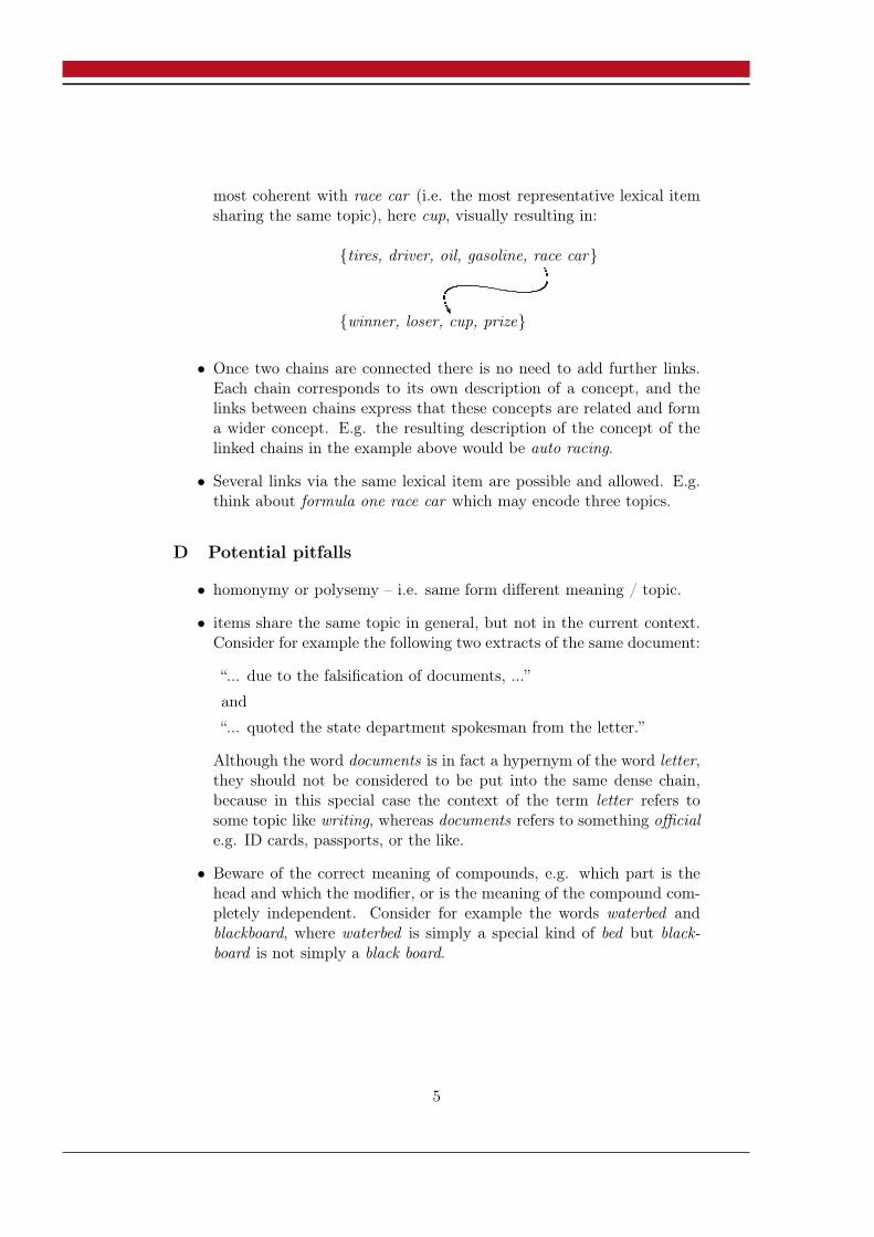
most coherent with race car (i.e. the most representative lexical itemsharing the same topic), here cup, visually resulting in:
{tires, driver, oil, gasoline, race car}
{winner, loser, cup, prize}U
• Once two chains are connected there is no need to add further links.Each chain corresponds to its own description of a concept, and thelinks between chains express that these concepts are related and forma wider concept. E.g. the resulting description of the concept of thelinked chains in the example above would be auto racing.
• Several links via the same lexical item are possible and allowed. E.g.think about formula one race car which may encode three topics.
D Potential pitfalls
• homonymy or polysemy – i.e. same form different meaning / topic.
• items share the same topic in general, but not in the current context.Consider for example the following two extracts of the same document:
“... due to the falsification of documents, ...”
and
“... quoted the state department spokesman from the letter.”
Although the word documents is in fact a hypernym of the word letter,they should not be considered to be put into the same dense chain,because in this special case the context of the term letter refers tosome topic like writing, whereas documents refers to something officiale.g. ID cards, passports, or the like.
• Beware of the correct meaning of compounds, e.g. which part is thehead and which the modifier, or is the meaning of the compound com-pletely independent. Consider for example the words waterbed andblackboard, where waterbed is simply a special kind of bed but black-board is not simply a black board.
5
Annotation recipe
read – grasp – search & merge – revisit & link
1. Read the document and grasp the main message behind the text.
2. Pick the next unchained lexical item as described in A.
3. Search for appropriate chains or other lexical items, and if they sharethe same topic as described in B merge them.
Remember that each item in the dense chain should satisfy the con-dition with every other item in the chain.
4. Continue with 2 until all lexical items in the text are served.
Remember that single item chains may exist.
5. Revisit the dense chains and check if you should do one of the followingoperations:
• splitting of chains – often chains grow too large because a toobroad topic was chosen.
• merging of chains – often too many chains emerge because a toonarrow topic was chosen.
6. Add links between dense chains via the lexical items as described in C.Try to pick meaningful representatives, because it often happensthat many items serve as candidate links. It is thus sufficient to linkchains only once. In other words, if a link exists between the chainsA and B there’s no need to seek for other links between A and B.
Remember that several links via the same lexical item are allowed.
When you are done, you ideally have one or two “big chains” (when consid-ering linked chains as a whole) describing the main message of the text, aswell as a few small chains describing side topics.
6
Examples
The following examples show selected texts from the Salsa corpus. Terms insquare brackets are preselected candidate lexical items (cf. schema sectionA). This preselection is done to ease the annotation process, schema Ain particular. These items are automatically selected based on a part-of-speech pattern and are not necessarily exact. However, in most cases thecandidate items are adequate enough and no effort must be put into findingadditional candidate items. Consider only correct items for chaining andlinking, though.
The examples comprise the original text with preselected candidate items,the identified dense chains and links including comments. The examplesare supplemental to the annotation recipe above and may still be arguable,though they might give a good direction to reach common ground.
7
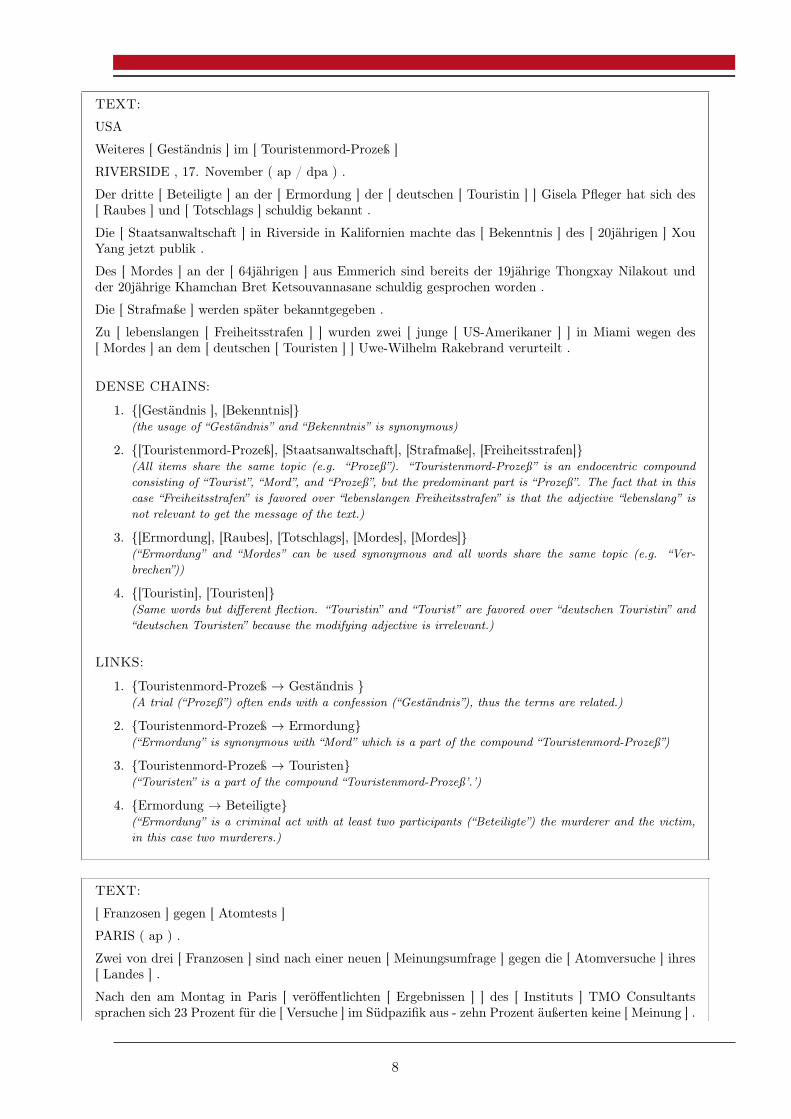
TEXT:
USA
Weiteres [ Geständnis ] im [ Touristenmord-Prozeß ]
RIVERSIDE , 17. November ( ap / dpa ) .
Der dritte [ Beteiligte ] an der [ Ermordung ] der [ deutschen [ Touristin ] ] Gisela Pfleger hat sich des[ Raubes ] und [ Totschlags ] schuldig bekannt .
Die [ Staatsanwaltschaft ] in Riverside in Kalifornien machte das [ Bekenntnis ] des [ 20jährigen ] XouYang jetzt publik .
Des [ Mordes ] an der [ 64jährigen ] aus Emmerich sind bereits der 19jährige Thongxay Nilakout undder 20jährige Khamchan Bret Ketsouvannasane schuldig gesprochen worden .
Die [ Strafmaße ] werden später bekanntgegeben .
Zu [ lebenslangen [ Freiheitsstrafen ] ] wurden zwei [ junge [ US-Amerikaner ] ] in Miami wegen des[ Mordes ] an dem [ deutschen [ Touristen ] ] Uwe-Wilhelm Rakebrand verurteilt .
DENSE CHAINS:
1. {[Geständnis ], [Bekenntnis]}(the usage of “Geständnis” and “Bekenntnis” is synonymous)
2. {[Touristenmord-Prozeß], [Staatsanwaltschaft], [Strafmaße], [Freiheitsstrafen]}(All items share the same topic (e.g. “Prozeß”). “Touristenmord-Prozeß” is an endocentric compoundconsisting of “Tourist”, “Mord”, and “Prozeß”, but the predominant part is “Prozeß”. The fact that in thiscase “Freiheitsstrafen” is favored over “lebenslangen Freiheitsstrafen” is that the adjective “lebenslang” isnot relevant to get the message of the text.)
3. {[Ermordung], [Raubes], [Totschlags], [Mordes], [Mordes]}(“Ermordung” and “Mordes” can be used synonymous and all words share the same topic (e.g. “Ver-brechen”))
4. {[Touristin], [Touristen]}(Same words but different flection. “Touristin” and “Tourist” are favored over “deutschen Touristin” and“deutschen Touristen” because the modifying adjective is irrelevant.)
LINKS:
1. {Touristenmord-Prozeß → Geständnis }(A trial (“Prozeß”) often ends with a confession (“Geständnis”), thus the terms are related.)
2. {Touristenmord-Prozeß → Ermordung}(“Ermordung” is synonymous with “Mord” which is a part of the compound “Touristenmord-Prozeß”)
3. {Touristenmord-Prozeß → Touristen}(“Touristen” is a part of the compound “Touristenmord-Prozeß’.’)
4. {Ermordung → Beteiligte}(“Ermordung” is a criminal act with at least two participants (“Beteiligte”) the murderer and the victim,in this case two murderers.)
TEXT:
[ Franzosen ] gegen [ Atomtests ]
PARIS ( ap ) .
Zwei von drei [ Franzosen ] sind nach einer neuen [ Meinungsumfrage ] gegen die [ Atomversuche ] ihres[ Landes ] .
Nach den am Montag in Paris [ veröffentlichten [ Ergebnissen ] ] des [ Instituts ] TMO Consultantssprachen sich 23 Prozent für die [ Versuche ] im Südpazifik aus - zehn Prozent äußerten keine [ Meinung ] .
8
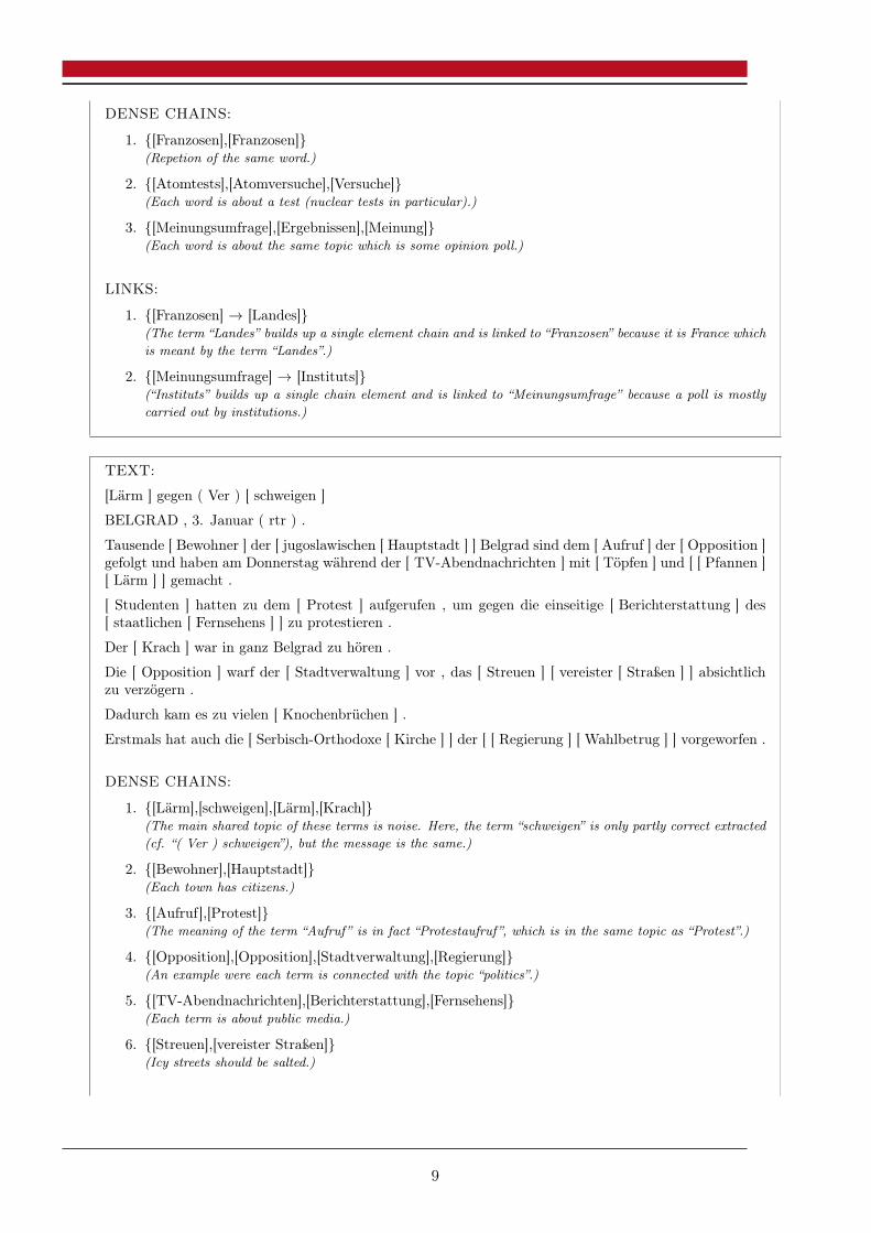
DENSE CHAINS:
1. {[Franzosen],[Franzosen]}(Repetion of the same word.)
2. {[Atomtests],[Atomversuche],[Versuche]}(Each word is about a test (nuclear tests in particular).)
3. {[Meinungsumfrage],[Ergebnissen],[Meinung]}(Each word is about the same topic which is some opinion poll.)
LINKS:
1. {[Franzosen] → [Landes]}(The term “Landes” builds up a single element chain and is linked to “Franzosen” because it is France whichis meant by the term “Landes”.)
2. {[Meinungsumfrage] → [Instituts]}(“Instituts” builds up a single chain element and is linked to “Meinungsumfrage” because a poll is mostlycarried out by institutions.)
TEXT:
[Lärm ] gegen ( Ver ) [ schweigen ]
BELGRAD , 3. Januar ( rtr ) .
Tausende [ Bewohner ] der [ jugoslawischen [ Hauptstadt ] ] Belgrad sind dem [ Aufruf ] der [ Opposition ]gefolgt und haben am Donnerstag während der [ TV-Abendnachrichten ] mit [ Töpfen ] und [ [ Pfannen ][ Lärm ] ] gemacht .
[ Studenten ] hatten zu dem [ Protest ] aufgerufen , um gegen die einseitige [ Berichterstattung ] des[ staatlichen [ Fernsehens ] ] zu protestieren .
Der [ Krach ] war in ganz Belgrad zu hören .
Die [ Opposition ] warf der [ Stadtverwaltung ] vor , das [ Streuen ] [ vereister [ Straßen ] ] absichtlichzu verzögern .
Dadurch kam es zu vielen [ Knochenbrüchen ] .
Erstmals hat auch die [ Serbisch-Orthodoxe [ Kirche ] ] der [ [ Regierung ] [ Wahlbetrug ] ] vorgeworfen .
DENSE CHAINS:
1. {[Lärm],[schweigen],[Lärm],[Krach]}(The main shared topic of these terms is noise. Here, the term “schweigen” is only partly correct extracted(cf. “( Ver ) schweigen”), but the message is the same.)
2. {[Bewohner],[Hauptstadt]}(Each town has citizens.)
3. {[Aufruf],[Protest]}(The meaning of the term “Aufruf” is in fact “Protestaufruf”, which is in the same topic as “Protest”.)
4. {[Opposition],[Opposition],[Stadtverwaltung],[Regierung]}(An example were each term is connected with the topic “politics”.)
5. {[TV-Abendnachrichten],[Berichterstattung],[Fernsehens]}(Each term is about public media.)
6. {[Streuen],[vereister Straßen]}(Icy streets should be salted.)
9
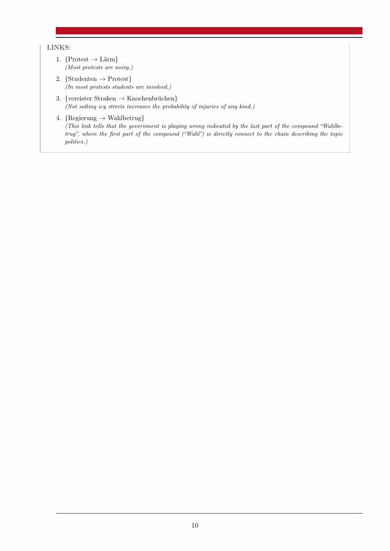
LINKS:
1. {Protest → Lärm}(Most protests are noisy.)
2. {Studenten → Protest}(In most protests students are involved.)
3. {vereister Straßen → Knochenbrüchen}(Not salting icy streets increases the probability of injuries of any kind.)
4. {Regierung → Wahlbetrug}(This link tells that the government is playing wrong indicated by the last part of the compound “Wahlbe-trug”, where the first part of the compound (“Wahl”) is directly connect to the chain describing the topicpolitics.)
10
110 B. Annotation Guidelines
C Annotation Guidelines Companion
111
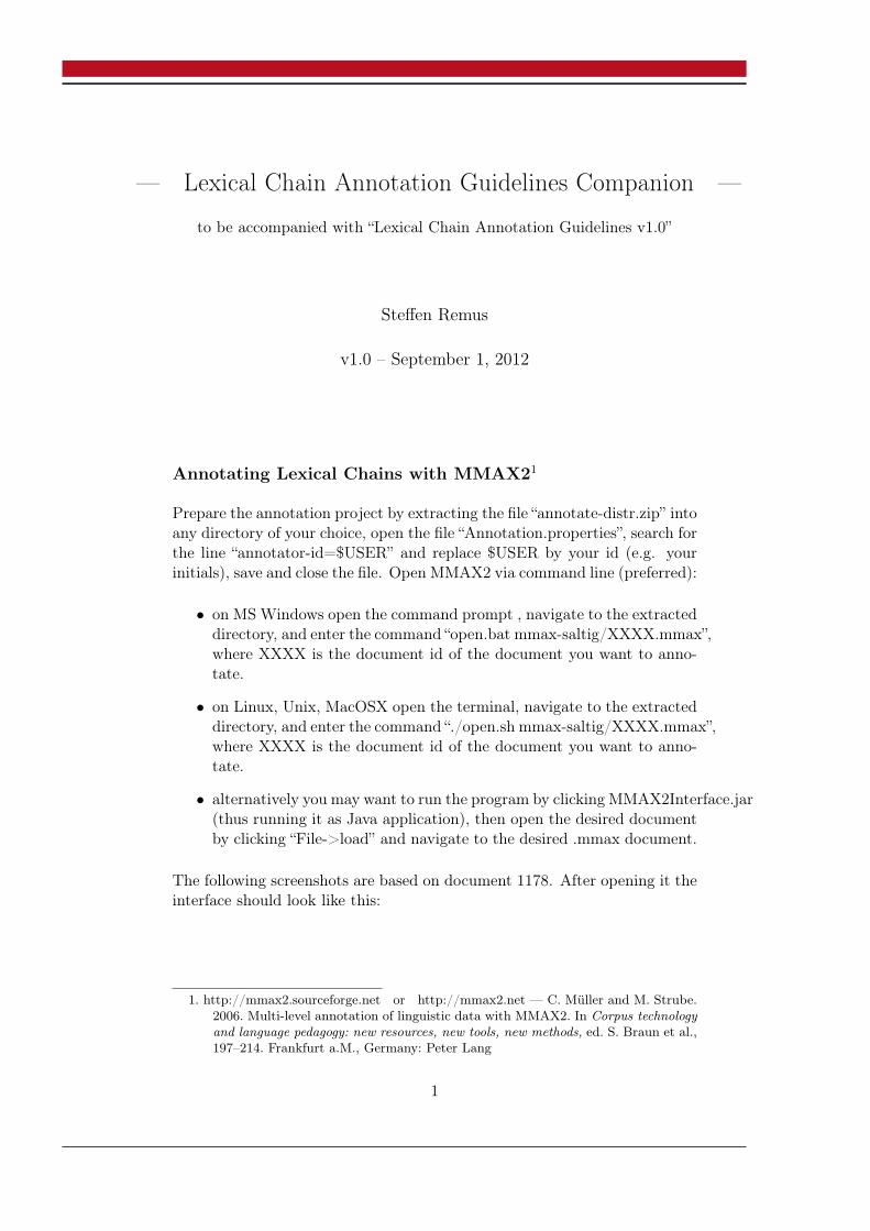
— Lexical Chain Annotation Guidelines Companion —
to be accompanied with “Lexical Chain Annotation Guidelines v1.0”
Steffen Remus
v1.0 – September 1, 2012
Annotating Lexical Chains with MMAX21
Prepare the annotation project by extracting the file “annotate-distr.zip” intoany directory of your choice, open the file “Annotation.properties”, search forthe line “annotator-id=$USER” and replace $USER by your id (e.g. yourinitials), save and close the file. Open MMAX2 via command line (preferred):
• on MS Windows open the command prompt , navigate to the extracteddirectory, and enter the command “open.bat mmax-saltig/XXXX.mmax”,where XXXX is the document id of the document you want to anno-tate.
• on Linux, Unix, MacOSX open the terminal, navigate to the extracteddirectory, and enter the command “./open.sh mmax-saltig/XXXX.mmax”,where XXXX is the document id of the document you want to anno-tate.
• alternatively you may want to run the program by clicking MMAX2Interface.jar(thus running it as Java application), then open the desired documentby clicking “File->load” and navigate to the desired .mmax document.
The following screenshots are based on document 1178. After opening it theinterface should look like this:
1. http://mmax2.sourceforge.net or http://mmax2.net — C. Müller and M. Strube.2006. Multi-level annotation of linguistic data with MMAX2. In Corpus technologyand language pedagogy: new resources, new tools, new methods, ed. S. Braun et al.,197–214. Frankfurt a.M., Germany: Peter Lang
1
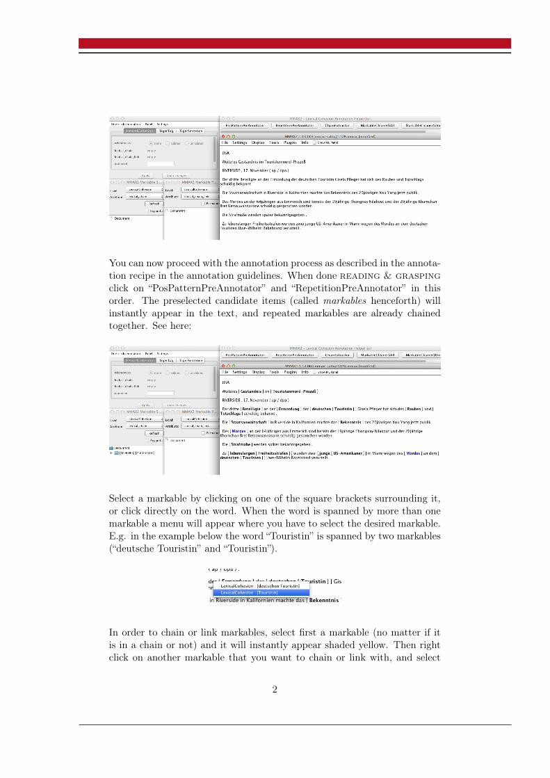
You can now proceed with the annotation process as described in the annota-tion recipe in the annotation guidelines. When done reading & graspingclick on “PosPatternPreAnnotator” and “RepetitionPreAnnotator” in thisorder. The preselected candidate items (called markables henceforth) willinstantly appear in the text, and repeated markables are already chainedtogether. See here:
Select a markable by clicking on one of the square brackets surrounding it,or click directly on the word. When the word is spanned by more than onemarkable a menu will appear where you have to select the desired markable.E.g. in the example below the word “Touristin” is spanned by two markables(“deutsche Touristin” and “Touristin”).
In order to chain or link markables, select first a markable (no matter if itis in a chain or not) and it will instantly appear shaded yellow. Then rightclick on another markable that you want to chain or link with, and select
2
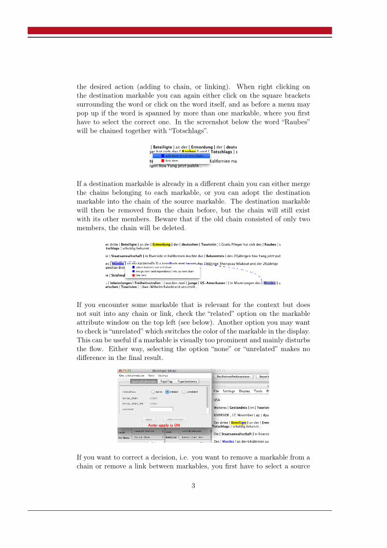
the desired action (adding to chain, or linking). When right clicking onthe destination markable you can again either click on the square bracketssurrounding the word or click on the word itself, and as before a menu maypop up if the word is spanned by more than one markable, where you firsthave to select the correct one. In the screenshot below the word “Raubes”will be chained together with “Totschlags”.
If a destination markable is already in a different chain you can either mergethe chains belonging to each markable, or you can adopt the destinationmarkable into the chain of the source markable. The destination markablewill then be removed from the chain before, but the chain will still existwith its other members. Beware that if the old chain consisted of only twomembers, the chain will be deleted.
If you encounter some markable that is relevant for the context but doesnot suit into any chain or link, check the “related” option on the markableattribute window on the top left (see below). Another option you may wantto check is “unrelated” which switches the color of the markable in the display.This can be useful if a markable is visually too prominent and mainly disturbsthe flow. Either way, selecting the option “none” or “unrelated” makes nodifference in the final result.
If you want to correct a decision, i.e. you want to remove a markable from achain or remove a link between markables, you first have to select a source
3
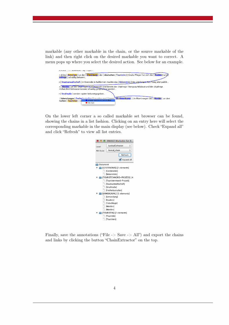
markable (any other markable in the chain, or the source markable of thelink) and then right click on the desired markable you want to correct. Amenu pops up where you select the desired action. See below for an example.
On the lower left corner a so called markable set browser can be found,showing the chains in a list fashion. Clicking on an entry here will select thecorresponding markable in the main display (see below). Check “Expand all”and click “Refresh” to view all list entries.
Finally, save the annotations (“File -> Save -> All”) and export the chainsand links by clicking the button “ChainExtractor” on the top.
4
Have Fun!
5
Recommended