Download pdf - Application of Actuarial Science to RAM - Home - Society ...srehsv.com/wp-content/uploads/2013/08/RAM-6-Final-1-Risk... · Application of Actuarial Science to RAM by Evan ... 20 0.001285

Application of Actuarial

Science to RAM

by Evan Leite, Luke Hankins,

Gene Hou, and Brian Saulino

Risk Lighthouse LLC

October 15, 2013

Contents

1) Actuarial Science

2) Project Data

3) Parametric Models

4) Risk Classification

5) Supply Simulation

October 30, 2013 www.risklighthouse.com 2

Actuarial Science


1

What is Actuarial Science?

October 30, 2013 4 www.risklighthouse.com

What is Actuarial Science?

• Actuarial Science – the discipline that applies mathematical and statistical methods to model and to assess risks, usually in insurance and finance.


What are Some Typical Actuarial Models?

• Occurrence Models – probability models that regress binomial occurrence versus transformed explanatory variables, i.e. Logit or Probit.

– Logit,

– Probit,


)'(logit 1

1

1

1)(

)()'(1

1

zee

xpkk

Kk zz

)'()(1 zxp


• Frequency Models – discrete count models that regress counts versus explanatory variables, i.e. Poisson.

– Poisson Model for Counts


... 2, 1, ,0 ,!

][ )( yy

eyYPy

)'( iz

i e


• Severity/Duration Models – continuous models that regress dollar amounts or time versus explanatory variables, i.e. Pareto, Weibull, Exponential.

– Exponential Model for Duration


The mean and standard deviation of an

exponential distribution are equal

What are Some Typical Actuarial Tools?

Period Life Table, 2007

Exact age

Male Female

Death probability a

Number of lives b

Life expectancy

Death probability a

Number of lives b

Life expectancy

0 0.007379 100,000 75.38 0.006096 100,000 80.43

1 0.000494 99,262 74.94 0.000434 99,390 79.92

2 0.000317 99,213 73.98 0.000256 99,347 78.95

3 0.000241 99,182 73.00 0.000192 99,322 77.97

4 0.000200 99,158 72.02 0.000148 99,303 76.99

5 0.000179 99,138 71.03 0.000136 99,288 76.00

6 0.000166 99,120 70.04 0.000128 99,275 75.01

7 0.000152 99,104 69.05 0.000122 99,262 74.02

8 0.000133 99,089 68.06 0.000115 99,250 73.03

9 0.000108 99,075 67.07 0.000106 99,238 72.04

10 0.000089 99,065 66.08 0.000100 99,228 71.04

11 0.000094 99,056 65.09 0.000102 99,218 70.05

12 0.000145 99,047 64.09 0.000120 99,208 69.06

13 0.000252 99,032 63.10 0.000157 99,196 68.07

14 0.000401 99,007 62.12 0.000209 99,180 67.08

15 0.000563 98,968 61.14 0.000267 99,160 66.09

16 0.000719 98,912 60.18 0.000323 99,133 65.11

17 0.000873 98,841 59.22 0.000369 99,101 64.13

18 0.001017 98,754 58.27 0.000401 99,064 63.15

19 0.001148 98,654 57.33 0.000422 99,025 62.18

20 0.001285 98,541 56.40 0.000441 98,983 61.20


http://www.ssa.gov/oact/STATS/table4c6.html




What are Some Typical Actuarial Tools?

Predictive Analytics for BIG DATA

Regression Based


Project Data


2

Can Actuarial Science be Applied to RAM?

• In early 2011, AMRDEC asked if Actuarial Science can be applied to enhance RAM initiatives.

• On the surface, the answer seems to be obvious. – Manipulate BIG DATA.

– Create life table for parts.

– Provide predictive analytics based on external environment factors.

• But…



• Part Life vs. Human Life (People Don’t Come Back)

Challenges

Pseudo Parts divided by failure


• 2410 Database – Copy 1,2,3

– Flight Hours, TailNo, Model, Dates, UIC, Time Since New, Time Since Last Install, Overhaul, Time Since Overhaul, etc.

• 1352 Database – TailNo, Dates, Hours by TailNo

• CBM HUMS database – TailNo, Dates, many environmental factors

• Intersection: TailNo & Date


Data Sets Used


Illustration of Survival-Type Data

Year Number in Study at

Beginning of Year

Number Died

During Year

Number Withdrawn

(Censored)

[0-1) 200 3 16

[1-2) 181 5 14

[2-3) 162 6 13

[3-4) 143 7 11

[4-5) 125 7 12

[5-6) 106 5 9

[6-7) 92 6 8

[7-8) 78 8 5

[8-9) 65 7 6

[9-10) 52 7 7

[10-11) 38 6 7

[11-12) 25 9 6

[12-13) 10 7 3 October 30, 2013 www.risklighthouse.com 17

Necessity to Account for Censored Data


Say we were asked to calculate the probability

that a patient would survive 5 years. One

incorrect way to calculate this probability is to

throw out the data from the withdrawn patients

(censored).

= 66.3% Chance to Survive 5 Years

Incorrect Method #1


Another incorrect way is use 200 as the initial

population, but to assume all the censoring falls

at the end of the study.

= 86.0% Chance to Survive 5 Years

Incorrect Method #2


Equation 1 leads to an overly pessimistic survival

probability, while equation 2 leads to an overly

optimistic survival probability.

The true survival probability is somewhere

between these two incorrect estimates. This

shows that statistical survival analysis techniques

are necessary.

Too optimistic or pessimistic?

Kaplan-Meier Estimator


The Kaplan–Meier estimator is the nonparametric maximum

likelihood estimate of the survival function, S(t). The Kaplan Meier

is different from the empirical distribution in that it can take into

account censored data.

tt i

ii

i n

dntS )(ˆKaplan-Meier Estimator :

ti ni di ci

0 15 0 0

2 15 2 1

3 12 1 2

5 9 1 1

10 7 2 0

Kaplan-Meier Estimator


Year Number in Study at

Beginning of Year

Number Died During

Year

Number Withdrawn

(Censored)

KM Survival

Function

[0-1) 200 3 16 98.5%

[1-2) 181 5 14 95.8%

[2-3) 162 6 13 92.2%

[3-4) 143 7 11 87.7%

[4-5) 125 7 12 82.8%

[5-6) 106 5 9 78.9%

[6-7) 92 6 8 73.8%

[7-8) 78 8 5 66.2%

[8-9) 65 7 6 59.1%

[9-10) 52 7 7 51.1%

[10-11) 38 6 7 43.0%

[11-12) 25 9 6 27.5%

[12-13) 10 7 3 8.3%


What is censored?

A censored observation occurs when the failure

condition is not met. For helicopter parts, are

we talking about supply or reliability?

We determine censoring by chargeable vs. non-

chargeable failure codes. Which failure codes

are chargeable for supply, and for reliability?


Supply Failure Event

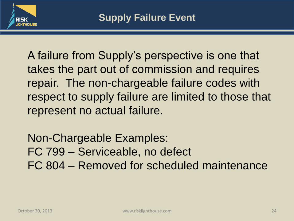
A failure from Supply’s perspective is one that

takes the part out of commission and requires

repair. The non-chargeable failure codes with

respect to supply failure are limited to those that

represent no actual failure.

Non-Chargeable Examples:

FC 799 – Serviceable, no defect

FC 804 – Removed for scheduled maintenance


Reliability Failure Event

A failure from Reliability’s perspective is one

that due to inherent properties of the part, rather

than environmental, combat, or misuse. The

non-chargeable failure codes with respect to

reliability failure include far more failure codes.

Non-Chargeable Examples:

FC 731: Battle Damage

FC 917: Bird Strike

REARM Engine


R.E.A.R.M.

Repair Event Analysis and Recording Machine

REARM Engine


•Uses the R statistical programming tool

•Input Excel 2410 and 1352 database

•Automatically correct (some) errors in data

•Output a list of clean sequences with

accompanying data

Parametric Distributions


3

Possible Distributions

• Normal

• Lognormal

• Exponential

• Beta

• Weibull

• Gamma

• Negative Binomial

• Cauchy


Possible Distributions


Survival Analysis Tools – KM Curves


Comparison of Parametric Survival Functions Zero-Truncated

Survival Regression


Survival Regression

Fits a parametric survival distribution to the model (Gaussian,

Weibull, Logistic, etc.)

Weibull CDF

This regression can fit a lambda (shape) to a survival distribution,

then adjust k (scale) to the effects of different covariates.

Weibull Parameters- Adjusting Scale


0

0.1

0.2

0.3

0.4

0.5

0.6

0.7

0.8

0.9

1

x 0.1 0.3 0.5 0.7 0.9 1.1 1.3 1.5 1.7 1.9 2.1 2.3 2.5 2.7 2.9 3.1 3.3 3.5 3.7 3.9

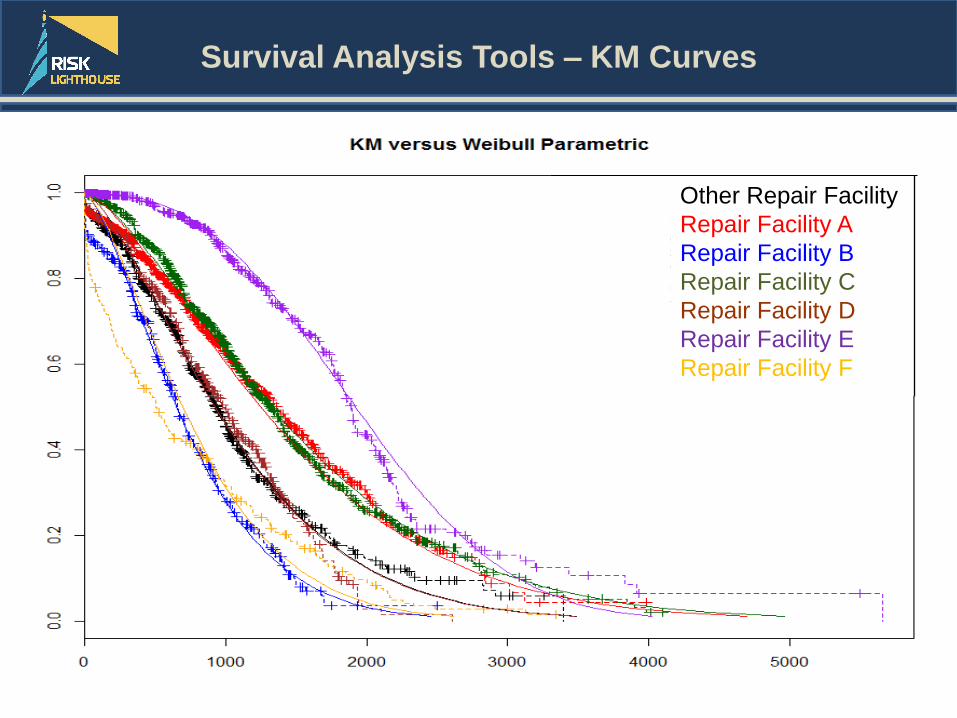
Survival Analysis Tools – KM Curves


Other Repair Facility

Repair Facility A

Repair Facility B

Repair Facility C

Repair Facility D

Repair Facility E

Repair Facility F

Flexible Survival Regression

• Parametric Models have advantages for – Prediction. – Extrapolation. – Quantification (e.g., absolute and relative differences in risk). – Modelling time-dependent effects. – Understanding. – Complex models in large datasets (time-dependent effects /multiple time-scales) – All cause, cause-specific or relative survival.

• The estimates obtained from flexible parametric survival models are incredibly similar to those obtained from a Cox model.

• An important feature of flexible parametric models is the ability • to model time-dependent effects, i.e., there are non-proportional • hazards

– Time-dependent effects are modeled using splines, but will – generally require fewer knots than the baseline. – This is because we are now modeling deviation from the baseline hazard rate. – Also possible to split time to estimate hazard ratio in different intervals.


Constructing the Flexible Parametric Model


• Piecewise Hazard Function

• No Continuity Corrections

• Function Forced to Join at Knots

• Continuous at First Derivative

• Continuous at Second Derivative

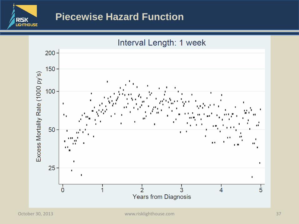
Piecewise Hazard Function


No Continuity Corrections


Function Forced to Join at Knots


Continuous at First Derivative


Continuous at Second Derivative


Risk Classification


4


Risk Classification Chart – Life Insurance

Category Preferred Standard Substandard

Smoking Non-Smokers Non-Smokers Smokers

Body Mass Index 18.5-24.9 25 to 29.9 Less than 18.5 Greater than 30

Driving Record No Tickets No Major Tickets (DWI)

Many Tickets or a Major Ticket

Conditional Inference

• Algorithm – Variable Selection Step 1:

• Permutation based significance test in order to select the variable,

• Choose the covariate with lowest p-value below than a pre-specified significance value, i.e. 0.05

– Choosing the p-value is a unique parameter which determines the size of the tree

– P-values are used to make comparisons between variables that are categorical and numerical

– Splitting Procedure Step 2: • Explore all possible splits

• Goodness of a split is evaluated again by a permutation –based test

– Recursively repeat steps 1 and 2 until no more splits can be determined


Conditional Inference Tree


Model 1

Top.Units

p < 0.001

1

{Other Unit, 1107TH AVCRAD, AVN MAINT BRANCH/SIKORSKY SUPP, CT-AVCRAD, DYNCORP ENHANCED ENG REP ACTY , PROTOTYPE ENGINEERING CO (CA), TRADOC (AL)}{CCAD, PARKER HANNIFIN CORP (CA), SIKORSKY, SIKORSKY (FL)}

Top.Model

p < 0.001

2

{EH-60A, HH-60L, MH-60K, MH-60L, UH-60A} {HH-60M, Other Model, UH-60L, UH-60M}

Node 3 (n = 1694)

0 1000 2000 3000 4000 5000

0

0.2

0.4

0.6

0.8

1Node 4 (n = 808)

0 1000 2000 3000 4000 5000

0

0.2

0.4

0.6

0.8

1

Top.Model

p < 0.001

5

{HH-60L, HH-60M, MH-60K, MH-60L, MH-60M, UH-60A, UH-60L} {EH-60A, Other Model, UH-60M}

Node 6 (n = 6305)

0 1000 2000 3000 4000 5000

0

0.2

0.4

0.6

0.8

1Node 7 (n = 1397)

0 1000 2000 3000 4000 5000

0

0.2

0.4

0.6

0.8

1

Age of Part

New Parts Old Parts

Repair Facility Model

Repair Facility A Not Repair Fac. A HH-60M, UH-60L,

or UH-60M Not HH-60M,

UH-60L, or UH-60M

Conditional Inference Tree


Model 5

Top.Units

p < 0.001

1

{Other Unit, 1107TH AVCRAD, AVN MAINT BRANCH/SIKORSKY SUPP, CT-AVCRAD, DYNCORP ENHANCED ENG REP ACTY , PROTOTYPE ENGINEERING CO (CA), TRADOC (AL)}{CCAD, PARKER HANNIFIN CORP (CA), SIKORSKY, SIKORSKY (FL)}

Top.Model

p < 0.001

2

{EH-60A, HH-60L, MH-60K, MH-60L, UH-60A} {HH-60M, Other Model, UH-60L, UH-60M}

Top.Units

p < 0.001

3

{CT-AVCRAD, DYNCORP ENHANCED ENG REP ACTY , TRADOC (AL)}{Other Unit, 1107TH AVCRAD, AVN MAINT BRANCH/SIKORSKY SUPP, PROTOTYPE ENGINEERING CO (CA)}

Node 4 (n = 691)

0 1000 2000 3000 4000 5000

0

0.2

0.4

0.6

0.8

1Node 5 (n = 1003)

0 1000 2000 3000 4000 5000

0

0.2

0.4

0.6

0.8

1Node 6 (n = 808)

0 1000 2000 3000 4000 5000

0

0.2

0.4

0.6

0.8

1

Top.Model

p < 0.001

7

{HH-60L, HH-60M, MH-60K, MH-60L, MH-60M, UH-60A, UH-60L} {EH-60A, Other Model, UH-60M}

Top.Units

p < 0.001

8

{CCAD, PARKER HANNIFIN CORP (CA), SIKORSKY (FL)} SIKORSKY

Node 9 (n = 5310)

0 1000 2000 3000 4000 5000

0

0.2

0.4

0.6

0.8

1Node 10 (n = 995)

0 1000 2000 3000 4000 5000

0

0.2

0.4

0.6

0.8

1Node 11 (n = 1397)

0 1000 2000 3000 4000 5000

0

0.2

0.4

0.6

0.8

1

Age of Part

New Parts Old Parts

Model Repair Facility

Not Repair Facility A Repair Facility A

Model

HH-60M, UH-60L, or UH-60M Not HH-60M,

UH-60L, or UH-60M

Repair Fac.

Repair Facility D or F Not Repair Fac. D or F EH-60A or UH-60M Not EH-60A or UH-60M

Cox Proportional Hazards Model


Alternatively, we can differentiate levels of risk factors using the

Cox Proportional Hazards model

The Cox Proportional Hazards model is as follows:

Where: is the hazard rate of a component i at time t,

is the baseline hazard rate at time t,

is the coefficient of the first covariate of interest,

is the first covariate of interest,

is the coefficient of second covariate of interest, and

is the second covariate of interest.

...)(0

2211*)()( XBXi ethth

)(thi

)(0 th

1

21X

2X

Difference in Hazard Rate by Repair Level


Cox Proportional Hazards by Previous Repair Level

n=12053 number of events=4113

Baseline = UH-60A

Beta exp(Beta) P-Value

MH-60K 0.19473 1.21498 0.00381 **

UH-60L -0.27767 0.75754 0.112

Significance codes: 0 ‘***’, 0.001 ‘**’, 0.01 ‘*’, 0.05 ‘.’

Constructing the Parametric Model

• Before the data of the old parts are fitted to the Weibull distribution, they are first split into 4 different classes (New, Preferred, Standard, and Substandard).

• The new parts with Times since new (TSN) values of zero are segmented from the other old parts and classified as new. For the old parts, they are classified as ether “preferred”, “standard”, or “substandard” depending on four risk factors.

• These four risk factors are: – Helicopter Model

– Previous Repair Facility

– Times since new (TSN)

– Previous Chargeable Failure Code

• RLH then uses the Cox Proportional Hazard Regression to measure the average hazard rate for each levels of the four risk factors and then rank them. The results are displayed on the next slide.



Risk Factors Rank Elements

Previous Repair Facility (UIC) Above, Above Average (AAA) UIC-A

Above Average (AA) UIC-B, UIC-C, UIC-D

Average (A) All Other UICs

Below Average (BA) UIC-F

Helicopter Model Above, Average (AA) HH-60G, EH-60L, UH-60M

Average (A) UH-60L and all other helicopter models

Below Average (BA) MH-60K

Previous Failure Code Average (A) Previous Failure Code is not 2 (Air Leak) or 520 (Pitted)

Below Average (BA) Previous Failure Code is 2 or 520

Time Since New (TSN) Above Average (AA) Less than 1500 flight hours

Average (A) Between 1500 and 3500 flight hours (inclusive)

Below Average (BA) Over 3500 flight hours




• There are 72 possible different combinations of these risk factors and each one is labeled as category 1,2, …., 72.

• The magnitude of each risk factor’s effect on survival rate may differ. The idea of creating these categories is to evaluate the overall effect of all four risk factors. These 72 categories are entered into a Cox PH regression equation with baseline set as category 32 and the results are shown in the next slide.

Category Previous UIC Time Since New

(TSN)

Previous Failure

Code

Model

8 AA A A AA

12 A AA A AA

32 (Baseline) A A A A



• The categories with a hazard rate that is lower than the baseline on average are put into the “Preferred” class, the categories with a hazard rate that is higher than the baseline on average are put into the “Substandard” class, and all other categories are put in the, “Standard” class. The new class contains all the new parts, regardless of their risk factors. RLH then constructed the parametric models by fitted the Weibull distribution to each of the four classes.

Class Categories Included Number of

Observations

Class

New All Parts with TSN = 0 4241 New

Preferred 7, 19, 20, 25, 26, 27 ,29, 31 1821 Preferred

Standard All Other Categories 3200 Standard

Substandard 33, 35, 36, 38, 44, 50 896 Substandard

Parametric Model: Goodness of Fit


0 500 1000 1500 2000 2500 3000 3500

0.0

0.2

0.4

0.6

0.8

1.0

Main Rotor Blades (All Classes) Weibul Distribution Fit (Supply Side)

Time to Failure (Fight Hours)

Pro

babi

lity

of F

ailu

re

Legend

Parametric Curve

New Class KM Curve N = 4098

Preferred Class KM Curve N = 3931

Standard Class KM Curve N = 3066

Substandard Class KM Curve N = 863

Parametric Model: Validation Testing


• The objective is to test if the four parametric models serves as an accurate representation of the real data.

• The “Train” data set, which 65% of the data randomly chosen, is fitted to a Weibull distribution to create a parametric model. The rest of the data, the “Test” data set, is used to plot a KM curve.

• The parametric curve is then compared with the KM curve.

• RLH then conducts the Kolmogorov-Smirnov (KS) Test between the KM and the parametric curve.

• The KS test can compare a sample data set with a reference distribution and determine the how likely that sample data is drawn from the reference distribution. In this case, the sample data is the “Test” data set and the reference distribution is the parametric model.


Results


0 500 1000 1500 2000 2500 3000

0.0

0.2

0.4

0.6

0.8

1.0

Main Rotor Blade Validation Test Results for Supply Side

Time To Failure

Su

rviv

al P

rob

ab

ility

Legend

(New)Train Data Set

(Preferred) Train Data Set

(Standard) Train Data Set

(Substandard) Train Data Set

Test Data Set


Results


• KS test results:

• The null hypothesis is that the sample data is drawn from the reference distribution. The results shows that the p-values for all four models are greater than the alpha, 0.05. Therefore, the null hypothesis is not rejected and the test indicates that the “Test” data set is likely to have been drawn from the parametric model.

Class Test Statistic (D) P-Value

New 0.0367 0.8355

Preferred 0.0262 0.9113

Standard 0.0356 0.8688

Substandard 0.0593 0.7655

Monte Carlo Method

And

Inventory Simulation


5

Monte Carlo Simulation Basics


Initial Conditions

Simulation

Process

Random

Number Input

Ending Condition

Repeat for

Duration

Repeat for Each

Simulation

Extract Mean,

VaR, TVaR

Monte Carlo Simulation Basics


http://genedan.com/tag/brownian-motion/

Heads - 50%

Tails - 50%

50 Flips per

Simulation

Simulation

Time

1 10

20

250

250




Simulation Basics: Value at Risk and

Conditional Value at Risk


In our simulation, assets might be considered to be spare inventory. http://www.nematrian.com/R.aspx?p=TailValueAtRisk

http://www.nematrian.com/R.aspx?p=TailValueAtRisk

Supply Simulation Initial Conditions

and Assumptions

• 200 Helicopters or ‘Slots’ of random frame composition

• 220 Parts with randomized covariates (TSLI, UIC)

• Method to classify parts into risk categories

• Hazard rate parameters for risk classes estimated from 2410

• Average flight hours per month for each airframe based on 1352 Dataset

_________________________________________________

• Monthly simulation, deaths/installs happen at end of month

• On failure parts have 20% chance of “True Death”

• Some failures are minor and repairs happen within a month


0 500 1000 1500 2000 2500 3000

0.0

10

.02

0.0

30

.04

Failure Probablility within 25 Flight Hours of current TSLI

TSLI

Ch

an

ce

of

Fa

ilu

re

Supply Simulation: Monthly Survival

• Since simulation is done in 1 month intervals, survivorship is only calculated assuming part survives the average flight hours per month of the airframe


0 500 1000 1500 2000 2500 3000 3500

0.0

0.2

0.4

0.6

0.8

1.0

Main Rotor Blades (All Classes) Weibul Distribution Fit (Reliability Side)

Time to Failure (Fight Hours)

Pro

ba

bility o

f F

ailu

re

Legend

Parametric Curve

New Class KM Curve N = 4085

Preferred Class KM Curve N = 3546

Standard Class KM Curve N = 3276

Substandard Class KM Curve N = 526

tPx = P(x + t | x + t > X) = S(x + t) / S(X)

tQx = 1 - tPx

S(x) tQx

Supply Simulation Process


3+ Months

2 Months

1 Month

Inventory

Install, Classify Risk, and

Determine Exposure (Flight Hours)

Simulate

Repair Queue

Recovery

True Death

<1 Month

Repair Time

Supply Simulation: Sample Run

and Results

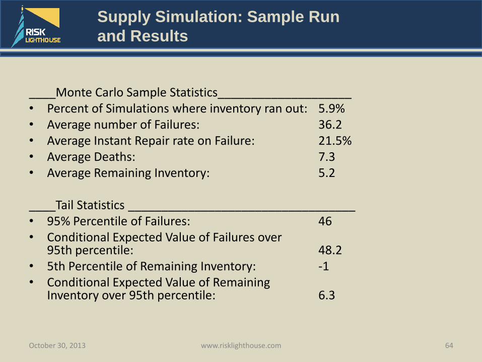
____Monte Carlo Sample Statistics____________________ • Percent of Simulations where inventory ran out: 5.9% • Average number of Failures: 36.2 • Average Instant Repair rate on Failure: 21.5% • Average Deaths: 7.3 • Average Remaining Inventory: 5.2

____Tail Statistics __________________________________ • 95% Percentile of Failures: 46 • Conditional Expected Value of Failures over

95th percentile: 48.2 • 5th Percentile of Remaining Inventory: -1 • Conditional Expected Value of Remaining

Inventory over 95th percentile: 6.3


Supply Simulation: Improvements

• Matching assumptions and process to general practices

• Reason for Failure (Specific Fail Code) – Associated distribution for repair times

• Nonchargeable removals – Allows parts to change helicopters without failing first

• Back testing Methods


Questions


4 What failure code is this!?

Thank you!


Contact Evan Leite

Suite 315

3405 Piedmont Road NE

Atlanta, GA 30305

Phone: 678-732-9112

[email protected]

www.risklighthouse.com

mailto:[email protected]

http://www.risklighthouse.com/