Download pdf - Analyzing a Prospective Red Wolf (Canis rufus) Reintroduction Site

1

Analyzing a Prospective Red Wolf (Canis rufus)

Reintroduction Site for Suitable Habitat

by Jon Shaffer

April, 2007

Abstract

Since its declared extinction in the wild in 1980, the red wolf has been reintroduced into

two areas of the South. The reintroduction in Northeastern North Carolina has been quite

successful, while the reintroduction into the Great Smoky Mountains National Park was

unsuccessful. The USFWS Red Wolf Recovery Plan calls for the additional establishment

of two more wild populations of wolves. I analyzed the potential of one prospective

release site to contain enough suitable habitat to support a reintroduction of red wolves.

The Central Coastal North Carolina area was chosen for analysis as it met general criteria

for the likely success of reintroduction, including a similar geography to the successful

Northeastern North Carolina site, and a large amount of land in conservation. ArcGIS 9.2

was used to identify core patches of potential habitat within the study area and calculate

the amount of their areas occurring on protected lands. The patches were examined for

connectivity using least-cost path analysis, and optimal corridors containing the top 5th

percentile best paths between patches were calculated. Three patches, that combined

would provide suitable habitat for wolf reintroduction, were identified. Together these

patches contained an area larger than the 68,800 hectares of habitat required for red wolf

reintroductions. And over 75 % of this area occurred on conservation lands. It is therefore

possible that the Central Coastal North Carolina area contains enough suitable habitat for

the reintroduction of red wolves. The approach used in this analysis could by applied to

other prospective red wolf release sites.

2

Introduction:

The red wolf (Canis rufus) was declared extinct in the wild in 1980. As a result of the

Endangered Species Act of 1973, the U.S. Fish and Wildlife Service (USFWS) initiated

the Red Wolf Recovery Program. It established a captive breeding program, and a

reintroduction plan with a goal of establishing at least three wild populations of wolves

totaling 220 animals; each population should occupy at least 178,000 acres (68,800

hectares) of contiguous habitat (USFWS 1990). Red wolves have been successfully

reintroduced into Northeastern North Carolina; there is currently a population of

approximately 100 centered among the Alligator River and Pocosin Lakes National

Wildlife Refuges. However, a similar reintroduction effort was unsuccessful in the Great

Smoky Mountains National Park (Kelly et al. 2004).

The USFWS is considering other prospective release sites for establishing additional red

wolf populations. Thirty one prospective release sites have been identified throughout the

former range of the red wolf (Van Manen et al. 2000). I will examine one of these

potential sites, the Central Coastal North Carolina area. The goal of my analysis is to

determine if this site contains enough physically suitable habitat to support a

reintroduction of red wolves. The site will be analyzed for the amount of core habitat it

contains, the connectivity of these areas, and the protection status of the core areas’ land.

An approach similar to that taken by Paquet et al. (1999) in their determination of habitat

suitability for gray wolf reintroduction in the Adirondacks will be used, with some

modifications to the methodology.

3

Methods:

Choice of site:

The Central Coastal North Carolina area consists of the land area, excluding barrier

islands, of four counties: Carteret, Craven, Jones, and Onslow (Figure 1). This site was

chosen for several reasons. First, it is geographically very similar to the northeastern

North Carolina site where red wolves have been successfully reintroduced. Next, it

contains several large protected areas of conservation lands including the Croatan

National Forest and the Hofmann State Forest. Third, the site has a low coyote density

compared to other areas of the state, and as much of the area is bounded by water, it may

be possible to exclude coyotes from the site. Coyotes present one of the greatest

challenges to the success of red wolf reintroductions as they readily hybridize with the

wolves, and can quickly dilute the gene pool (Kelly et al. 2004, Phillips et al. 2003).

Finally, the close proximity of the study site to the successful reintroduction site in

Northeastern North Carolina will allow for easier exchange of resources, expertise, and

personnel between reintroduction areas.

Data:

The National Elevation Dataset (1 arc second) and National Land Cover Dataset 2001

from the USGS were used to determine elevation and land cover at the site. Highway,

county boundary, state boundary, and waterbody vector data were obtained from the

USGS National Atlas of the United States. Vector data on municipal town boundaries and

roads were obtained from the North Carolina Flood Mapping Program. Vector data on

4

protected conservation lands were obtained from the North Carolina Corporate

Geographic Database’s “Lands Managed for Conservation and Open Space” data layer

(NCCGDB 2003). Deer density data were obtained from the North Carolina Wildlife

Resources Commission. The ranges of red wolf populations reintroduced into the Great

Smoky Mountains and Northeastern North Carolina were obtained in the form of vector

data from NatureServe (Patterson et al. 2003). All data were projected to NAD 1983

UTM Zone 18N and most layers were clipped to the four county research site. All raster

data throughout the analysis were set to a 30 by 30 meter resolution.

Analysis:

Analysis was conducted in ArcMap 9.2 (See Appendix for models and Python Scripts).

Patches of core habitat for red wolves were identified in the study area based on the

following criteria:

1. Road density of less than 0.25 km/km2.

2. 1 km from highways.

3. 2 km from incorporated towns.

4. Land cover of one of the following classes: deciduous, evergreen, or mixed forest,

shrub/scrub, grassland/herbaceous, woody wetlands, or emergent herbaceous

wetlands.

5. Deer density of at least 5 deer/km2.

6. Slopes no greater than 20o.

7. Patch area of at least 45.6 km2.

5

Low human density and distance from roads are among the most important predictors of

potential red wolf habitat in North Carolina (Kelly et al. 2004). Following the model of

Patterson et al. (2003), road density was used as an approximation of human density.

Road density was calculated by converting the roads data into a raster and calculating

focal statistics on a moving 1km by 1km window. The highway and town data were

buffered and combined into a raster of unsuitable habitat. The land cover data were

reclassified to reflect the habitat preferences of red wolves depicted above. Deer are the

most important prey item for red wolves, accounting for 43% of the biomass digested by

wolves in Northeastern North Carolina (Phillips et al. 2003). As such, a raster was

created from the deer data identifying areas with a deer density of at least 5 deer/km2. As

slopes greater than 20o may be avoided by wolves (Callaghan 1999), a slope raster was

created from the elevation data.

The above raster layers were combined to create a raster of potential habitat patches.

Then habitat patches with an area of at least 45.6 km2 were extracted from this raster to

create the core habitat patches raster. The area of 45.6 km2 represents the minimum home

range size for a pack of red wolves (Phillips et al. 2003). The area of core habitat patches

existing on protected conservation land was then extracted and tabulated.

Least-cost path analysis was used to examine functional connectivity between core

habitat areas. A raster cost surface reflecting the variable resistance to wolf movement

was created. Each value of the raster represented how much relative cost a wolf would

6

face when traveling through each 30 by 30 meter pixel. The cost surface was generated

from a composite of three different cost rasters: land cover cost, road density cost, and

highways cost. Table 1 displays the features associated with these rasters and their

respective costs. Estimates of the relative costs of different features were adapted from

Paquet et al. (1999) when possible and estimated from knowledge gleaned from the

literature on wolves. The minimal cost distance from core habitat patches was then

calculated through the cost surface. Allocation boundaries were drawn at the locations

where the maximum least-cost distance occurred between any two core patches. The cells

along each allocation boundary with the minimum 5% of cost distance values were then

used (as described by Theobald 2006) to create multiple pathways and a corresponding

corridor containing the top 5th

percentile best paths between patches.

Results:

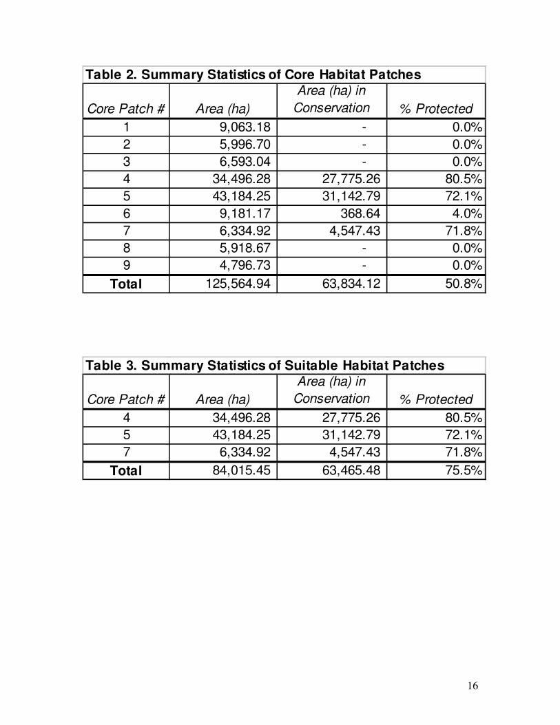
Nine core patches of habitat were identified in the study area (Fig. 2). These ranged in

size from 48 to 432 km2 (Table 2). Three of the core patches (4, 5, and 7) were better

connected to each other than the other patches; these other patches tended to lay along the

periphery of the study area. The lower cost distances between these three patches can be

seen in Figure 3. Much of the land in patches 4, 5, and 7 had the added benefit of existing

under conservation protection (Croatan National Forest and Hofmann State Forest), while

almost none of the land in the other core patches was protected (Table 2). Most of the

7

likely corridors between core patches did not lie on protected land. The exception to this

was the corridor between patches 5 and 7, which occurred almost completely on

conservation lands (Fig. 4).

Discussion:

In light of the large cost distances between many of the potential core habitat patches,

their relatively small size, and their peripheral location where they may be less protected

from coyote immigration, it is recommended that only the three central, connected

patches be considered as suitable habitat (patches 4, 5, and 7). This selection includes the

two largest habitat patches and has the added benefit of being mostly contained within

conservation lands. Taken together these patches have an area of 84.0 km2 (Table 3). This

meets the reintroduction requirement of 170,000 acres (68.8 km2) of wolf habitat.

Especially encouraging is that over 75% of this suitable habitat occurs on protected

conservation lands, and the most likely corridors between two of the patches are

protected.

There were several limitations to this analysis. First, it did not take coyote density into

account. Hybridization with coyotes is the one of the greatest challenges to successful red

wolf reintroduction, and it was one of the main factors preventing the success of the

Great Smoky Mountain reintroduction effort (Kelly et al. 2004, Phillips et al. 2003).

Anecdotally, coyote density is low in the study area, but actual numbers need to be

8

accurately surveyed. Another limitation to the study was the use of land cover data that is

several years old. Although this is the most recent data available, the study site is located

in a fast growing area of North Carolina and faces continuing development pressure. A

third limitation is the subjectivity involved in the estimation of cost for the cost surfaces.

Actual costs of movement for wolves over certain surfaces may be much different than

those estimated. Also, it is tough to determine the magnitude of cost distance at which

travel between two core patches of habitat becomes unlikely or impossible. But, as more

information is gleaned from telemetry and behavioral studies we can update the relative

costs of movement in the model.

Though there are limitations, this geospatial approach provides a useful framework for

determining if the prospective reintroduction site will provide suitable wolf habitat. It is

flexible in that costs can be adjusted and more variables added as more data are obtained

regarding the habitat needs of the red wolf. On the basis of this study, it appears quite

possible that the Central Coastal North Carolina area contains enough suitable habitat for

the reintroduction of red wolves. I recommend that this site be analyzed further for

consideration for red wolf reintroduction. The models used in this approach may be

useful when analyzing other prospective reintroduction sites for the red wolf.

9

10

11

12

13

References:

Callaghan, C., Paquet, P.C. and Wierzchowski J. 1999. Highway effects on Gray Wolves

within the Golden Canyon, British Columbia. ICOWET III, The International

Conference on Wildlife Ecology and Transportation, Missoula, USA.

Kelly, B.T., Beyer A. and Phillips, M.K. 2004. Red Wolf Canis rufus. Pp. 87–92 in C.

Sillero-Zubiri, M. Hoffmann and D.W. Macdonald, eds. Canids: foxes, wolves,

jackals and dogs. Status survey and conservation action plan. Gland and

Cambridge: IUCN/SSC.

Paquet, P.C., Strittholt, J.R. and Staus, N.L. 1999. Wolf reintroduction feasibility in the

Adirondack Park. Prepared for the Adirondack Citizens Advisory Committee on

the Feasibility of Wolf Reintroduction. Conservation Biology Institute, Corvallis,

OR, USA.

Phillips, M.K., Henry, V.G. and Kelly, B.T. 2003. Restoration of the red wolf. Pp. 272–

288 in L.D. Mech and L. Boitani, eds. Wolves: behavior, ecology and

conservation. University of Chicago Press, Chicago, IL, USA.

Theobald, D.M. 2006. Exploring the functional connectivity of landscapes using

landscape networks. Pp. 416-443 in K.R. Crooks and M.A. Sanjayan, eds.

Connectivity conservation: Maintaining connections for nature. Cambridge

University Press.

U.S. Fish and Wildlife Service. 1990. Red wolf recovery and species survival plan. U.S.

Fish and Wildlife Service, Atlanta, GA, USA.

Van Manen, F.T., Crawford, B.A. and Clark, J.D. 2000. Predicting red wolf release

success in the southeastern United States. Journal Of Wildlife Management

64:895–902.

Data Sources:

National Atlas of the United States. County Boundaries, 2001. 2005.

National Atlas of the United States. Roads. 1999.

National Atlas of the United States. State Boundaries. 2005.

National Atlas of the United States. Streams and Waterbodies. 2005.

14

North Carolina Corporate Geographic Database (NCCGDB). Lands Managed for

Conservation and Open Space. N.C. Center for Geographic Information and

Analysis, 2003.

North Carolina Floodplain Mapping Program. Municipal Area. 2001.

North Carolina Floodplain Mapping Program. Roads. 2001.

Patterson, B. D., G. Ceballos, W. Sechrest, M. F. Tognelli, T. Brooks, L. Luna, P. Ortega,

I. Salazar, and B. E. Young. 2003. Digital Distribution Maps of the Mammals of

the Western Hemisphere, version 1.0. NatureServe, Arlington, Virginia, USA.

U.S. Geological Survey (USGS). National Land Cover Characterization 2001.

U.S. Geological Survey (USGS). USGS National Elevation Data Set. 2003.

Acknowledgements:

I would like to thank the North Carolina Wildlife Resources Commission for providing

me with deer density data. I would also like to thank Dr. Jennifer Swenson for allowing

me to turn this report in late.

15

Table 1. Cost Surface Assignment for Study Site

Landcover Surface Cost

Open Water 10

Developed, Open Space 8

Developed, Low Intensity 10

Developed, Medium Intensity No Data

Developed, High Intensity No Data

Barren Land 8

Deciduous Forest 1

Evergreen Forest 1

Mixed Forest 1

Shrub/Scrub 1

Grassland/Herbaceous 3

Pasture/Hay 6

Cultivated Crops 7

Woody Wetlands 1

Herbaceous Wetlands 1

Road Density Surface (km/km 2 ) Cost

0 - 0.25 0

0.25 - 0.5 5

> 0.5 10

Highway Surface Cost

Highway Presence 5

Highway Absence 0

16

Table 2. Summary Statistics of Core Habitat Patches

Core Patch # Area (ha)

Area (ha) in

Conservation % Protected

1 9,063.18 - 0.0%

2 5,996.70 - 0.0%

3 6,593.04 - 0.0%

4 34,496.28 27,775.26 80.5%

5 43,184.25 31,142.79 72.1%

6 9,181.17 368.64 4.0%

7 6,334.92 4,547.43 71.8%

8 5,918.67 - 0.0%

9 4,796.73 - 0.0%

Total 125,564.94 63,834.12 50.8%

Table 3. Summary Statistics of Suitable Habitat Patches

Core Patch # Area (ha)

Area (ha) in

Conservation % Protected

4 34,496.28 27,775.26 80.5%

5 43,184.25 31,142.79 72.1%

7 6,334.92 4,547.43 71.8%

Total 84,015.45 63,465.48 75.5%

17

Appendix A: Data Preparation Model and Scripts

18

# Import system modules

import sys, string, os, arcgisscripting

# Create the Geoprocessor object

gp = arcgisscripting.create()

# Set the necessary product code

gp.SetProduct("ArcInfo")

# Check out any necessary licenses

gp.CheckOutExtension("spatial")

# Load required toolboxes...

gp.AddToolbox("C:/Program Files/ArcGIS/ArcToolbox/Toolboxes/Spatial

Analyst Tools.tbx")

gp.AddToolbox("C:/Program Files/ArcGIS/ArcToolbox/Toolboxes/Conversion

Tools.tbx")

gp.AddToolbox("C:/Program Files/ArcGIS/ArcToolbox/Toolboxes/Data

Management Tools.tbx")

gp.AddToolbox("C:/Program Files/ArcGIS/ArcToolbox/Toolboxes/Analysis

Tools.tbx")

# Set the Geoprocessing environment...

gp.cellSize = "z:\\classes\\ENV261\\Project\\Data\\landuse"

gp.mask = "z:\\classes\\ENV261\\Project\\Data\\landuse"

# Local variables...

Roads = "z:\\classes\\ENV261\\Project\\scratch\\roads"

roads__2_ = "z:\\classes\\ENV261\\Project\\scratch\\roads"

Municipal2_shp =

"z:\\classes\\ENV261\\Project\\scratch\\Municipal2.shp"

Municipal_shp__2_ =

"z:\\classes\\ENV261\\Project\\scratch\\Municipal2.shp"

ned_92187551 = "ned_92187551"

v61246557_tif = "61246557.tif"

Highway_shp = "z:\\classes\\ENV261\\Project\\Highway.shp"

DEM = "z:\\classes\\ENV261\\Project\\dem"

Landcover = "z:\\classes\\ENV261\\Project\\Landcover"

Counties_shp = "z:\\classes\\ENV261\\Project\\Counties.shp"

Roads16_shp = "z:\\classes\\ENV261\\Project\\NC_flood\\Roads16.shp"

















19





road_proj_shp = "z:\\classes\\ENV261\\Project\\road_proj.shp"

roadways_shp = "z:\\classes\\ENV261\\Project\\Data\\roadways.shp"

Site_shp = "z:\\classes\\ENV261\\Project\\Data\\Site.shp"

elevation = "z:\\classes\\ENV261\\Project\\Data\\elevation"

landuse = "z:\\classes\\ENV261\\Project\\Data\\landuse"

Municipal_area10_shp =

"z:\\classes\\ENV261\\Project\\NC_flood\\Municipal_area10.shp"

































Municipal2_Project_shp =

"z:\\classes\\ENV261\\Project\\scratch\\Municipal2_Project.shp"

towns_shp = "z:\\classes\\ENV261\\Project\\Data\\towns.shp"

v61253372_shp =

"z:\\classes\\ENV261\\Project\\shapefiles\\streams\\61253372.shp"

Stream = "z:\\classes\\ENV261\\Project\\Data\\Stream"

Highway_study_shp =

"z:\\classes\\ENV261\\Project\\Data\\Highway_study.shp"

v26828739_shp =

"z:\\classes\\ENV261\\Project\\shapefiles\\waterbodies\\26828739.shp"

Waterbody = "z:\\classes\\ENV261\\Project\\Data\\Waterbody"


roadshape_shp = "z:\\classes\\ENV261\\Project\\scratch\\roadshape.shp"

road1 = "z:\\classes\\ENV261\\Project\\scratch\\road1"

20

Reclass_road = "z:\\classes\\ENV261\\Project\\scratch\\Reclass_road"

FocalSt_Recl1 = "z:\\classes\\ENV261\\Project\\scratch\\focalst_recl1"

local_dens = "z:\\classes\\ENV261\\Project\\scratch\\local_dens"

towns_Buffer_shp =

"z:\\classes\\ENV261\\Project\\scratch\\towns_Buffer.shp"

slope__2_ = "z:\\classes\\ENV261\\Project\\Data\\slope"

Highway_buffer_shp =

"z:\\classes\\ENV261\\Project\\scratch\\Highway_buffer.shp"

buffers_shp = "z:\\classes\\ENV261\\Project\\scratch\\buffers.shp"

buffer = "z:\\classes\\ENV261\\Project\\scratch\\buffer"

lmcos0902_shp =

"z:\\classes\\ENV261\\Project\\Conservation\\Cons\\lmcos0902.shp"

Protected_shp = "z:\\classes\\ENV261\\Project\\Data\\Protected.shp"

Conserve_shp = "z:\\classes\\ENV261\\Project\\Data\\Conserve.shp"

Highway = "z:\\classes\\ENV261\\Project\\scratch\\highway"

statesp020 = "statesp020"

statesp020__2_ = "statesp020"

statesp020__3_ = "statesp020"

NC2 = "z:\\classes\\ENV261\\Project\\scratch\\NC2"

v79131492_shp =

"z:\\classes\\ENV261\\Project\\shapefiles\\counties_east\\79131492.shp"

v73121562_shp =

"z:\\classes\\ENV261\\Project\\shapefiles\\roads_east\\73121562.shp"

deer_shp = "z:\\classes\\ENV261\\Project\\scratch\\deer.shp"

deer_raster = "z:\\classes\\ENV261\\Project\\scratch\\deer_raster"

deer_rast_prj = "z:\\classes\\ENV261\\Project\\scratch\\deer_rast_prj"

cani_rufu_pl_shp = "z:\\classes\\ENV261\\Project\\shapefiles\\red

wolf\\cani_rufu_pl.shp"

canis_ruf_proj =

"z:\\classes\\ENV261\\Project\\scratch\\canis_ruf_proj"

cani_rufu_pl_shp__2_ = "z:\\classes\\ENV261\\Project\\shapefiles\\red

wolf\\cani_rufu_pl.shp"

Output_Feature_Class =

"z:\\classes\\ENV261\\Project\\scratch\\canis_ruf_proj_Clip1.shp"

north_carolina_shp__2_ =

"z:\\classes\\ENV261\\Project\\scratch\\north_carolina.shp"

# Process: Feature Class To Coverage...

gp.FeatureclassToCoverage_conversion("z:\\classes\\ENV261\\Project\\NC_

flood\\Roads17.shp

ROUTE;z:\\classes\\ENV261\\Project\\NC_flood\\Roads16.shp

















21




ROUTE;z:\\classes\\ENV261\\Project\\NC_flood\\Roads22.shp ROUTE",

Roads, "", "DOUBLE")

# Process: Define Projection...

gp.DefineProjection_management(Roads,

"PROJCS['NAD_1983_StatePlane_North_Carolina_FIPS_3200_Feet',GEOGCS['GCS

_North_American_1983',DATUM['D_North_American_1983',SPHEROID['GRS_1980'

,6378137.0,298.257222101]],PRIMEM['Greenwich',0.0],UNIT['Degree',0.0174

532925199433]],PROJECTION['Lambert_Conformal_Conic'],PARAMETER['False_E

asting',2000000.002616666],PARAMETER['False_Northing',0.0],PARAMETER['C

entral_Meridian',-

79.0],PARAMETER['Standard_Parallel_1',34.33333333333334],PARAMETER['Sta

ndard_Parallel_2',36.16666666666666],PARAMETER['Latitude_Of_Origin',33.

75],UNIT['Foot_US',0.3048006096012192]]")

# Process: Project (4)...

gp.Project_management(v79131492_shp, Counties_shp,

"PROJCS['NAD_1983_UTM_Zone_18N',GEOGCS['GCS_North_American_1983',DATUM[

'D_North_American_1983',SPHEROID['GRS_1980',6378137.0,298.257222101]],P

RIMEM['Greenwich',0.0],UNIT['Degree',0.0174532925199433]],PROJECTION['T

ransverse_Mercator'],PARAMETER['False_Easting',500000.0],PARAMETER['Fal

se_Northing',0.0],PARAMETER['Central_Meridian',-

75.0],PARAMETER['Scale_Factor',0.9996],PARAMETER['Latitude_Of_Origin',0

.0],UNIT['Meter',1.0]]", "",

"GEOGCS['GCS_North_American_1983',DATUM['D_North_American_1983',SPHEROI

D['GRS_1980',6378137.0,298.257222101]],PRIMEM['Greenwich',0.0],UNIT['De

gree',0.0174532925199433]]")


gp.Project_management(v61253372_shp, Stream,







.0],UNIT['Meter',1.0]]", "",



gree',0.0174532925199433]]")


gp.Project_management(v26828739_shp, Waterbody,







.0],UNIT['Meter',1.0]]", "",



gree',0.0174532925199433]]")

22


gp.Project_management(roadshape_shp, road_proj_shp,







.0],UNIT['Meter',1.0]]", "",






entral_Meridian',-



75],UNIT['Foot_US',0.3048006096012192]]")

# Process: Clip...

gp.Clip_analysis(road_proj_shp, Site_shp, roadways_shp, "")


gp.ProjectRaster_management(v61246557_tif, Landcover,







.0],UNIT['Meter',1.0]];-5120900 -9998100

450445547.391054;#;#;0.001;#;#;IsHighPrecision", "NEAREST", "30", "",

"",

"PROJCS['USA_Contiguous_Albers_Equal_Area_Conic_USGS_version',GEOGCS['G

CS_North_American_1983',DATUM['D_North_American_1983',SPHEROID['GRS_198

0',6378137.0,298.257222101]],PRIMEM['Greenwich',0.0],UNIT['Degree',0.01

74532925199433]],PROJECTION['Albers'],PARAMETER['False_Easting',0.0],PA

RAMETER['False_Northing',0.0],PARAMETER['Central_Meridian',-

96.0],PARAMETER['Standard_Parallel_1',29.5],PARAMETER['Standard_Paralle

l_2',45.5],PARAMETER['Latitude_Of_Origin',23.0],UNIT['Meter',1.0]];-

16901100 -6972200 266467840.990852;#;#;0.001;#;#;IsHighPrecision")

# Process: Extract by Mask (2)...

gp.ExtractByMask_sa(Landcover, Site_shp, landuse)

# Process: Feature to Raster...

gp.FeatureToRaster_conversion(roadways_shp, "LPOLY_", road1, landuse)

# Process: Reclassify...

gp.Reclassify_sa(road1, "VALUE", "0 1;NODATA 0", Reclass_road, "DATA")

# Process: Focal Statistics...

gp.FocalStatistics_sa(Reclass_road, FocalSt_Recl1, "Rectangle 1000 1000

MAP", "SUM", "DATA")

# Process: Single Output Map Algebra...

23

gp.SingleOutputMapAlgebra_sa("z:\\classes\\ENV261\\Project\\scratch\\fo

calst_recl1*0.03", local_dens,

"z:\\classes\\ENV261\\Project\\scratch\\focalst_recl1")


gp.ProjectRaster_management(ned_92187551, DEM,







.0],UNIT['Meter',1.0]];-5120900 -9998100

450445547.391054;#;#;0.001;#;#;IsHighPrecision", "NEAREST", "<Null>",

"", "",



gree',0.0174532925199433]],VERTCS['Unknown VCS from ArcInfo

Workstation',VDATUM['Unknown'],PARAMETER['Vertical_Shift',0.0],PARAMETE

R['Direction',1.0],UNIT['Meter',1.0]];-400 -400

11258999068426.2;#;#;8.98315284119521E-09;#;#;IsHighPrecision")

# Process: Extract by Mask...

gp.ExtractByMask_sa(DEM, Site_shp, elevation)

# Process: Slope...

tempEnvironment0 = gp.cellSize


gp.Slope_sa(elevation, slope__2_, "DEGREE", "1")

gp.cellSize = tempEnvironment0

# Process: Union...

gp.Union_analysis("z:\\classes\\ENV261\\Project\\NC_flood\\Municipal_ar

ea10.shp #;z:\\classes\\ENV261\\Project\\NC_flood\\Municipal_area11.shp

#;z:\\classes\\ENV261\\Project\\NC_flood\\Municipal_area12.shp














#;z:\\classes\\ENV261\\Project\\NC_flood\\Municipal_area9.shp #",

Municipal2_shp, "ALL", "", "GAPS")

# Process: Define Projection (2)...

gp.DefineProjection_management(Municipal2_shp,





24


entral_Meridian',-



75],UNIT['Foot_US',0.3048006096012192]]")


gp.Project_management(Municipal_shp__2_, Municipal2_Project_shp,







.0],UNIT['Meter',1.0]]", "",






entral_Meridian',-



75],UNIT['Foot_US',0.3048006096012192]]")

# Process: Clip (2)...

gp.Clip_analysis(Municipal2_Project_shp, Site_shp, towns_shp, "")

# Process: Buffer (2)...

tempEnvironment0 = gp.newPrecision

gp.newPrecision = "SINGLE"

tempEnvironment1 = gp.XYResolution

gp.XYResolution = ""

tempEnvironment2 = gp.scratchWorkspace

gp.scratchWorkspace = "z:\\classes\\ENV261\\Project\\scratch"

tempEnvironment3 = gp.MTolerance

gp.MTolerance = ""

tempEnvironment4 = gp.randomGenerator

gp.randomGenerator = "0 ACM599"

tempEnvironment5 = gp.outputCoordinateSystem

gp.outputCoordinateSystem = ""

tempEnvironment6 = gp.projectCompare

gp.projectCompare = "NONE"

tempEnvironment7 = gp.outputZFlag

gp.outputZFlag = "Same As Input"

tempEnvironment8 = gp.qualifiedFieldNames

gp.qualifiedFieldNames = "true"

tempEnvironment9 = gp.extent

gp.extent = "DEFAULT"

tempEnvironment10 = gp.XYTolerance

gp.XYTolerance = ""

tempEnvironment11 = gp.outputZValue

gp.outputZValue = ""

tempEnvironment12 = gp.outputMFlag

gp.outputMFlag = "Same As Input"

tempEnvironment13 = gp.geographicTransformations

gp.geographicTransformations = ""

25

tempEnvironment14 = gp.ZResolution

gp.ZResolution = ""

tempEnvironment15 = gp.workspace

gp.workspace = "z:\\classes\\ENV261\\Project\\Data"

tempEnvironment16 = gp.MResolution

gp.MResolution = ""

tempEnvironment17 = gp.derivedPrecision

gp.derivedPrecision = "HIGHEST"

tempEnvironment18 = gp.ZTolerance

gp.ZTolerance = ""

gp.Buffer_analysis(towns_shp, towns_Buffer_shp, "2 Kilometers", "FULL",

"ROUND", "ALL", "")

gp.newPrecision = tempEnvironment0

gp.XYResolution = tempEnvironment1

gp.scratchWorkspace = tempEnvironment2

gp.MTolerance = tempEnvironment3

gp.randomGenerator = tempEnvironment4

gp.outputCoordinateSystem = tempEnvironment5

gp.projectCompare = tempEnvironment6

gp.outputZFlag = tempEnvironment7

gp.qualifiedFieldNames = tempEnvironment8

gp.extent = tempEnvironment9

gp.XYTolerance = tempEnvironment10

gp.outputZValue = tempEnvironment11

gp.outputMFlag = tempEnvironment12

gp.geographicTransformations = tempEnvironment13

gp.ZResolution = tempEnvironment14

gp.workspace = tempEnvironment15

gp.MResolution = tempEnvironment16

gp.derivedPrecision = tempEnvironment17

gp.ZTolerance = tempEnvironment18

# Process: Project...

gp.Project_management(v73121562_shp, Highway_shp,







.0],UNIT['Meter',1.0]]", "",



gree',0.0174532925199433]]")


gp.Clip_analysis(Highway_shp, Site_shp, Highway_study_shp, "")

# Process: Buffer (3)...

gp.Buffer_analysis(Highway_study_shp, Highway_buffer_shp, "1

Kilometers", "FULL", "ROUND", "NONE", "")

# Process: Union (2)...

gp.Union_analysis("z:\\classes\\ENV261\\Project\\scratch\\towns_Buffer.

shp #;z:\\classes\\ENV261\\Project\\scratch\\Highway_buffer.shp #",

buffers_shp, "ALL", "", "GAPS")

26

# Process: Feature to Raster (2)...

tempEnvironment0 = gp.cellSize


tempEnvironment1 = gp.mask

gp.mask = "z:\\classes\\ENV261\\Project\\Data\\landuse"

gp.FeatureToRaster_conversion(buffers_shp, "Id", buffer, "30")

gp.cellSize = tempEnvironment0

gp.mask = tempEnvironment1


gp.Project_management(lmcos0902_shp, Conserve_shp,







.0],UNIT['Meter',1.0]]", "",

"PROJCS['NAD_1983_StatePlane_North_Carolina_FIPS_3200',GEOGCS['GCS_Nort

h_American_1983',DATUM['D_North_American_1983',SPHEROID['GRS_1980',6378

137.0,298.257222101]],PRIMEM['Greenwich',0.0],UNIT['Degree',0.017453292

5199433]],PROJECTION['Lambert_Conformal_Conic'],PARAMETER['False_Eastin

g',609601.22],PARAMETER['False_Northing',0.0],PARAMETER['Central_Meridi

an',-



75],UNIT['Meter',1.0]]")


gp.Clip_analysis(Conserve_shp, Site_shp, Protected_shp, "")

# Process: Feature to Raster (3)...

gp.FeatureToRaster_conversion(Highway_study_shp, "NAME", Highway, "30")


gp.DefineProjection_management(statesp020,



gree',0.0174532925199433]]")

# Process: Select Layer By Attribute...

gp.SelectLayerByAttribute_management(statesp020__2_, "NEW_SELECTION",

"\"STATE\" = 'North Carolina'")

# Process: Polygon to Raster...

gp.PolygonToRaster_conversion(deer_shp, "Dens_km", deer_raster,

"CELL_CENTER", "NONE", "30")


gp.ProjectRaster_management(deer_raster, deer_rast_prj,







.0],UNIT['Meter',1.0]];-5120900 -9998100

27

450445547.391054;#;#;0.001;#;#;IsHighPrecision", "NEAREST", "30", "",

"",







.0],UNIT['Meter',1.0]];-5120900 -9998100

450445547.391054;#;#;0.001;#;#;IsHighPrecision")


gp.DefineProjection_management(cani_rufu_pl_shp,



gree',0.0174532925199433]]")


gp.Project_management(cani_rufu_pl_shp__2_, canis_ruf_proj,







.0],UNIT['Meter',1.0]]", "",



gree',0.0174532925199433]]")


gp.Project_management(north_carolina_shp__2_, NC2,







.0],UNIT['Meter',1.0]]", "",



gree',0.0174532925199433]]")


gp.Clip_analysis(canis_ruf_proj, NC2, Output_Feature_Class, "")

28

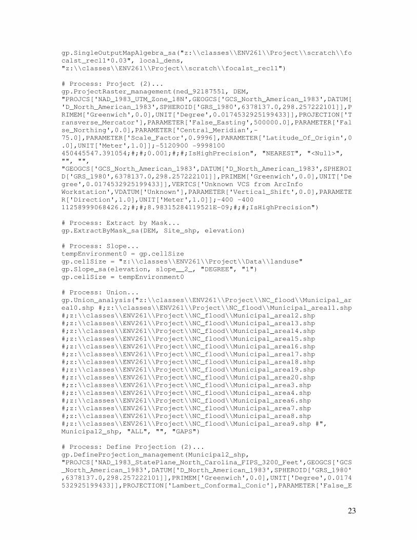
Appendix B: Analysis Model and Scripts

29

# Import system modules

import sys, string, os, arcgisscripting

# Create the Geoprocessor object

gp = arcgisscripting.create()

# Check out any necessary licenses

gp.CheckOutExtension("spatial")

# Load required toolboxes...

gp.AddToolbox("C:/Program Files/ArcGIS/ArcToolbox/Toolboxes/Spatial

Analyst Tools.tbx")

gp.AddToolbox("C:/Program Files/ArcGIS/ArcToolbox/Toolboxes/Conversion

Tools.tbx")

# Set the Geoprocessing environment...

gp.XYResolution = ""

gp.scratchWorkspace = "z:\\classes\\ENV261\\Project\\scratch"

gp.MTolerance = ""

gp.randomGenerator = "0 ACM599"

gp.outputCoordinateSystem = ""

gp.outputZFlag = "Same As Input"

gp.qualifiedFieldNames = "true"

gp.extent = "798393.534402281 3818666.10197191 931413.534402281

3926216.10197191"

gp.XYTolerance = ""

gp.cellSize = "30"

gp.outputZValue = ""

gp.outputMFlag = "Same As Input"

gp.geographicTransformations = ""

gp.ZResolution = ""

gp.mask = "landuse"

gp.workspace = "z:\\classes\\ENV261\\Project\\Data"

gp.MResolution = ""

gp.ZTolerance = ""

# Local variables...

buffer = "z:\\classes\\ENV261\\Project\\scratch\\buffer"

landuse = "z:\\classes\\ENV261\\Project\\Data\\landuse"

local_dens = "z:\\classes\\ENV261\\Project\\scratch\\local_dens"

landcov_cor = "z:\\classes\\ENV261\\Project\\scratch\\landcov_cor"

buffer_recl = "z:\\classes\\ENV261\\Project\\scratch\\buffer_recl"

dens_reclass = "z:\\classes\\ENV261\\Project\\scratch\\dens_reclass"

slope_recl = "z:\\classes\\ENV261\\Project\\scratch\\slope_recl"

habitat = "z:\\classes\\ENV261\\Project\\Data\\habitat"

patches = "z:\\classes\\ENV261\\Project\\scratch\\patches"

core = "z:\\classes\\ENV261\\Project\\Data\\core"

core_patches = "z:\\classes\\ENV261\\Project\\Data\\core_patches"

landuse__2_ = "z:\\classes\\ENV261\\Project\\Data\\landuse"

land_cost = "z:\\classes\\ENV261\\Project\\scratch\\land_cost"

cost_alloc = "z:\\classes\\ENV261\\Project\\scratch\\cost_alloc"

cost_distance = "z:\\classes\\ENV261\\Project\\Data\\cost_distance"

cost_backlink = "z:\\classes\\ENV261\\Project\\Data\\cost_backlink"

Focal_Var = "z:\\classes\\ENV261\\Project\\scratch\\Focal_Var"

Alloc_Ridg = "z:\\classes\\ENV261\\Project\\Data\\Alloc_Ridg"

ridgmin = "z:\\classes\\ENV261\\Project\\scratch\\ridgmin"

30

Ridge_Range = "z:\\classes\\ENV261\\Project\\scratch\\Ridge_Range"

lw_5p_ridg = "z:\\classes\\ENV261\\Project\\scratch\\lw_5p_ridg"

low5_rg = "z:\\classes\\ENV261\\Project\\scratch\\low5_rg"

costpath = "z:\\classes\\ENV261\\Project\\Data\\costpath"

road_cost = "z:\\classes\\ENV261\\Project\\scratch\\road_cost"

highway = "z:\\classes\\ENV261\\Project\\scratch\\highway"

highway_cost = "z:\\classes\\ENV261\\Project\\scratch\\highway_cost"

cost_surface = "z:\\classes\\ENV261\\Project\\scratch\\cost_surface"

slope__2_ = "z:\\classes\\ENV261\\Project\\Data\\slope"

protect_core = "z:\\classes\\ENV261\\Project\\scratch\\protect_core"

Protected_shp = "z:\\classes\\ENV261\\Project\\Data\\Protected.shp"

deer_rast_prj = "Z:\\classes\\ENV261\\Project\\scratch\\deer_rast_prj"

Reclass_deer = "z:\\classes\\ENV261\\Project\\scratch\\Reclass_deer"

corridor_shp = "z:\\classes\\ENV261\\Project\\Data\\corridor.shp"

# Process: Reclassify (2)...

gp.Reclassify_sa(buffer, "VALUE", "0 NODATA;NODATA 0", buffer_recl,

"DATA")


gp.Reclassify_sa(slope__2_, "Value", "0 20 0;20 30 NODATA", slope_recl,

"DATA")

# Process: Reclassify...

gp.Reclassify_sa(landuse, "VALUE", "11 NODATA;21 NODATA;21 24 NODATA;24

31 NODATA;41 43 0;43 52 0;52 71 0;81 82 NODATA;90 95 0", landcov_cor,

"DATA")


gp.Reclassify_sa(local_dens, "Value", "0 0.25 0;0.25 17.600000000000001

NODATA", dens_reclass, "DATA")


gp.Reclassify_sa(deer_rast_prj, "Value", "0 NODATA;0 5 NODATA;5

17.374500274658203 0", Reclass_deer, "DATA")

# Process: Single Output Map Algebra...

gp.SingleOutputMapAlgebra_sa("z:\\classes\\ENV261\\Project\\scratch\\bu

ffer_recl+z:\\classes\\ENV261\\Project\\scratch\\dens_reclass+z:\\class

es\\ENV261\\Project\\scratch\\slope_recl+z:\\classes\\ENV261\\Project\\

scratch\\landcov_cor +

z:\\classes\\ENV261\\Project\\scratch\\reclass_deer", habitat,

"z:\\classes\\ENV261\\Project\\scratch\\buffer_recl;z:\\classes\\ENV261

\\Project\\scratch\\slope_recl;z:\\classes\\ENV261\\Project\\scratch\\l

andcov_cor;z:\\classes\\ENV261\\Project\\scratch\\dens_reclass;z:\\clas

ses\\ENV261\\Project\\scratch\\Reclass_deer")

# Process: Region Group...

gp.RegionGroup_sa(habitat, patches, "FOUR", "WITHIN", "ADD_LINK", "")


gp.Reclassify_sa(patches, "COUNT", "1 50666 NODATA;50667 500000 0",

core, "DATA")

# Process: Region Group (2)...

gp.RegionGroup_sa(core, core_patches, "FOUR", "WITHIN", "ADD_LINK", "")

31

# Process: Extract by Mask...

gp.ExtractByMask_sa(core_patches, Protected_shp, protect_core)


gp.Reclassify_sa(local_dens, "Value", "0 0.25 0;0.25 0.5 5;0.5

17.600000000000001 10", road_cost, "DATA")


gp.Reclassify_sa(highway, "VALUE", "1 14 5;NODATA 0", highway_cost,

"DATA")


gp.Reclassify_sa(landuse__2_, "VALUE", "11 10;21 8;22 10;23 NODATA;24

NODATA;31 8;41 52 1;71 3;81 6;82 7;90 95 1", land_cost, "DATA")

# Process: Single Output Map Algebra (3)...

gp.SingleOutputMapAlgebra_sa("z:\\classes\\ENV261\\Project\\scratch\\hi

ghway_cost + z:\\classes\\ENV261\\Project\\scratch\\land_cost +

z:\\classes\\ENV261\\Project\\scratch\\road_cost", cost_surface,

"z:\\classes\\ENV261\\Project\\scratch\\road_cost;z:\\classes\\ENV261\\

Project\\scratch\\highway_cost;z:\\classes\\ENV261\\Project\\scratch\\l

and_cost")

# Process: Cost Allocation (2)...

gp.CostAllocation_sa(core_patches, cost_surface, cost_alloc, "", "",

"VALUE", cost_distance, cost_backlink)

# Process: Focal Statistics...

gp.FocalStatistics_sa(cost_alloc, Focal_Var, "Rectangle 3 3 CELL",

"VARIETY", "DATA")

# Process: Set Null...

gp.SetNull_sa(Focal_Var, cost_alloc, Alloc_Ridg, "\"VALUE\" = 1")

# Process: Zonal Statistics...

gp.ZonalStatistics_sa(Alloc_Ridg, "VALUE", cost_distance, ridgmin,

"MINIMUM", "DATA")

# Process: Zonal Statistics (2)...

gp.ZonalStatistics_sa(Alloc_Ridg, "VALUE", cost_distance, Ridge_Range,

"RANGE", "DATA")

# Process: Single Output Map Algebra (2)...

gp.SingleOutputMapAlgebra_sa("Con(cost_distance <= (ridgmin +

(Ridge_Range / 20)) , 1)

", lw_5p_ridg,

"z:\\classes\\ENV261\\Project\\scratch\\ridgmin;z:\\classes\\ENV261\\Pr

oject\\scratch\\Ridge_Range;z:\\classes\\ENV261\\Project\\Data\\cost_di

stance")

# Process: Region Group (3)...

gp.RegionGroup_sa(lw_5p_ridg, low5_rg, "EIGHT", "WITHIN", "ADD_LINK",

"")

# Process: Cost Path...

gp.CostPath_sa(low5_rg, cost_distance, cost_backlink, costpath,

"EACH_CELL", "VALUE")

32

# Process: Raster to Polyline...

gp.RasterToPolyline_conversion(costpath, corridor_shp, "ZERO", "0",

"SIMPLIFY", "VALUE").