Algorithm Design Using Spectral Graph Theory
Richard Peng
CMU-CS-13-121August 2013
School of Computer ScienceCarnegie Mellon University
Pittsburgh, PA 15213
Thesis Committee:Gary L. Miller, Chair
Guy E. BlellochAlan Frieze
Daniel A. Spielman, Yale University
Submitted in partial fulfillment of the requirementsfor the degree of Doctor of Philosophy.
Copyright © 2013 Richard Peng
This research was supported in part by the National Science Foundation under grant number CCF-1018463, by aMicrosoft Research PhD Fellowship, by the National Eye Institute under grant numbers R01-EY01317-08 and RO1-EY11289-22, and by the Natural Sciences and Engineering Research Council of Canada under grant numbers M-377343-2009 and D-390928-2010. Parts of this work were done while at Microsoft Research New England. Anyopinions, findings, and conclusions or recommendations expressed in this material are those of the author and do notnecessarily reflect the views of the funding parties.

Keywords: Combinatorial Preconditioning, Linear System Solvers, Spectral Graph Theory,Parallel Algorithms, Low Stretch Embeddings, Image Processing

To my parents and grandparents

iv

Abstract
Spectral graph theory is the interplay between linear algebra and combinatorialgraph theory. Laplace’s equation and its discrete form, the Laplacian matrix, appearubiquitously in mathematical physics. Due to the recent discovery of very fast solversfor these equations, they are also becoming increasingly useful in combinatorial opti-mization, computer vision, computer graphics, and machine learning.
In this thesis, we develop highly efficient and parallelizable algorithms for solv-ing linear systems involving graph Laplacian matrices. These solvers can also beextended to symmetric diagonally dominant matrices and M -matrices, both of whichare closely related to graph Laplacians. Our algorithms build upon two decades ofprogress on combinatorial preconditioning, which connects numerical and combinato-rial algorithms through spectral graph theory. They in turn rely on tools from numeri-cal analysis, metric embeddings, and random matrix theory.
We give two solver algorithms that take diametrically opposite approaches. Thefirst is motivated by combinatorial algorithms, and aims to gradually break the prob-lem into several smaller ones. It represents major simplifications over previous solverconstructions, and has theoretical running time comparable to sorting. The second ismotivated by numerical analysis, and aims to rapidly improve the algebraic connectiv-ity of the graph. It is the first highly efficient solver for Laplacian linear systems thatparallelizes almost completely.
Our results improve the performances of applications of fast linear system solversranging from scientific computing to algorithmic graph theory. We also show thatthese solvers can be used to address broad classes of image processing tasks, and givesome preliminary experimental results.

vi

Acknowledgments
This thesis is written with the help of many people. First and foremost I would like to thankmy advisor, Gary Miller, who introduced me to most of the topics discussed here and helped methroughout my studies at CMU. My thesis committee members, Guy Blelloch, Alan Frieze, andDaniel Spielman, provided me with invaluable advice during the dissertation process. I am alsograteful towards Ian Munro and Daniel Sleator for their constant guidance.
I am indebted to the co-authors who I had the fortune to work with during my graduate studies.Many of the ideas and results in this thesis are due to collaborations with Yiannis Koutis, KanatTangwongsan, Hui Han Chin, and Shen Chen Xu. Michael Cohen, Jakub Pachocki, and ShenChen Xu also provided very helpful comments and feedback on earlier versions of this document.I was fortunate to be hosted by Aleksander Madry and Madhu Sudan while interning at MicrosoftResearch New England. While there, I also had many enlightening discussions with JonathanKelner and Alex Levin.
I would like to thank my parents and grandparents who encouraged and cultivated my interests;and friends who helped me throughout graduate school: Bessie, Eric, Hui Han, Mark, Neal, Tom,and Travis. Finally, I want to thank the CNOI, CEMC, IOI, USACO, and SGU for developingmy problem solving abilities, stretching my imagination, and always giving me something to lookforward to.
vii

viii

Contents
1 Introduction 1
1.1 Graphs and Linear Systems . . . . . . . . . . . . . . . . . . . . . . . . . . . . . . 1
1.2 Related Work . . . . . . . . . . . . . . . . . . . . . . . . . . . . . . . . . . . . . 4
1.3 Structure of This Thesis . . . . . . . . . . . . . . . . . . . . . . . . . . . . . . . . 6
1.4 Applications . . . . . . . . . . . . . . . . . . . . . . . . . . . . . . . . . . . . . . 8
1.5 Solving Linear Systems . . . . . . . . . . . . . . . . . . . . . . . . . . . . . . . . 9
1.6 Matrices and Similarity . . . . . . . . . . . . . . . . . . . . . . . . . . . . . . . . 14
2 Nearly O(m log n) Time Solver 23
2.1 Reductions in Graph Size . . . . . . . . . . . . . . . . . . . . . . . . . . . . . . . 23
2.2 Ultra-Sparsification Algorithm . . . . . . . . . . . . . . . . . . . . . . . . . . . . 26
2.3 Recursive Preconditioning and Nearly-Linear Time Solvers . . . . . . . . . . . . . 30
2.4 Reuse, Recycle, and Reduce the Tree . . . . . . . . . . . . . . . . . . . . . . . . . 34
2.5 Tighter Bound for High Stretch Edges . . . . . . . . . . . . . . . . . . . . . . . . 36
2.6 Stability Under Fixed Point Arithmetic . . . . . . . . . . . . . . . . . . . . . . . . 39
3 Polylog Depth, Nearly-Linear Work Solvers 47
3.1 Overview of Our Approach . . . . . . . . . . . . . . . . . . . . . . . . . . . . . . 49
3.2 Parallel Solver . . . . . . . . . . . . . . . . . . . . . . . . . . . . . . . . . . . . . 51
3.3 Nearly-Linear Sized Parallel Solver Chains . . . . . . . . . . . . . . . . . . . . . 55
3.4 Alternate Construction of Parallel Solver Chains . . . . . . . . . . . . . . . . . . . 63
4 Construction of Low-Stretch Subgraphs 75
4.1 Low Stretch Spanning Trees and Subgraphs . . . . . . . . . . . . . . . . . . . . . 76
4.2 Parallel Partition Routine . . . . . . . . . . . . . . . . . . . . . . . . . . . . . . . 79
ix

4.3 Parallel Construction of Low Stretch Subgraphs . . . . . . . . . . . . . . . . . . . 88
4.4 Construction of low `α-stretch spanning trees . . . . . . . . . . . . . . . . . . . . 93
5 Applications to Image Processing 955.1 Background and Formulations . . . . . . . . . . . . . . . . . . . . . . . . . . . . 97
5.2 Applications . . . . . . . . . . . . . . . . . . . . . . . . . . . . . . . . . . . . . . 99
5.3 Related Algorithms . . . . . . . . . . . . . . . . . . . . . . . . . . . . . . . . . . 101
5.4 Approximating Grouped Least Squares Using Quadratic Minimization . . . . . . . 102
5.5 Evidence of Practical Feasibility . . . . . . . . . . . . . . . . . . . . . . . . . . . 111
5.6 Relations between Graph Problems and Minimizing LASSO Objectives . . . . . . 112
5.7 Other Variants . . . . . . . . . . . . . . . . . . . . . . . . . . . . . . . . . . . . . 116
5.8 Remarks . . . . . . . . . . . . . . . . . . . . . . . . . . . . . . . . . . . . . . . . 117
6 Conclusion and Open Problems 1196.1 Low Stretch Spanning Trees . . . . . . . . . . . . . . . . . . . . . . . . . . . . . 119
6.2 Interaction between Iterative Methods and Sparsification . . . . . . . . . . . . . . 120
Bibliography 120
A Deferred Proofs 133
B Spectral Sparsification by Sampling 135B.1 From Matrix Chernoff Bounds to Sparsification Guarantees . . . . . . . . . . . . . 136
B.2 Proof of Concentration Bound . . . . . . . . . . . . . . . . . . . . . . . . . . . . 137
C Partial Cholesky Factorization 145C.1 Partial Cholesky Factorization on Graph Laplacians . . . . . . . . . . . . . . . . . 146
C.2 Errors Under Partial Cholesky Factorization . . . . . . . . . . . . . . . . . . . . . 147
D Iterative Methods 155D.1 Richardson Iteration . . . . . . . . . . . . . . . . . . . . . . . . . . . . . . . . . . 155
D.2 Chebyshev Iteration . . . . . . . . . . . . . . . . . . . . . . . . . . . . . . . . . . 158
D.3 Chebyshev Iteration with Round-off Errors . . . . . . . . . . . . . . . . . . . . . 163
x

List of Figures
1.1 Representing a social network as a graph. . . . . . . . . . . . . . . . . . . . . . . 2
1.2 A resistive electric network with resistors labeled by their conductances (f) . . . . 3
1.3 Call structure of a 3-level W-cycle algorithm corresponding to the runtime recur-rence given in Equation 1.5 with t = 2. Each level makes 2 calls in succession toa problem that’s 4 times smaller. . . . . . . . . . . . . . . . . . . . . . . . . . . . 12
1.4 Call structure of a 3-level V-cycle algorithm. Each level makes 1 calls to a problemof comparable size. A small number of levels leads to a fast algorithm. . . . . . . . 14
2.1 The effective resistance RT (e) of the blue off-tree edge in the red tree is 1/4 +1/5 + 1/2 = 0.95. Its stretch strT (e) = weRT (e) is (1/4 + 1/5 + 1/2)/(1/2) = 1.9 27
4.1 Cycle on n vertices. Any tree T can include only n−1 of these edges. If the graphis unweighted, the remaining edge has stretch n− 1. . . . . . . . . . . . . . . . . 77
4.2 Two possible spanning trees of the unit weighted square grid, shown with rededges. . . . . . . . . . . . . . . . . . . . . . . . . . . . . . . . . . . . . . . . . . 77
4.3 Low stretch spanning tree for the square grid (in red) with extra edges of highstretch (narrower, in green). These edges can be viewed either as edges to beresolved later in the recursive algorithm, or as forming a subgraph along with thetree . . . . . . . . . . . . . . . . . . . . . . . . . . . . . . . . . . . . . . . . . . 79
5.1 Outputs of various denoising algorithms on image with AWGN noise. From left toright: noisy version, Split Bregman [GO09], Fixed Point [MSX11], and GroupedLeast Squares. Errors listed below each figure from left to right are `2 and `1 normsof differences with the original. . . . . . . . . . . . . . . . . . . . . . . . . . . . 111
5.2 Applications to various image processing tasks. From left to right: image segmen-tation, global feature extraction / blurring, and decoloring. . . . . . . . . . . . . . 113
5.3 Example of seamless cloning using Poisson Image Editing . . . . . . . . . . . . . 114
xi

xii

Chapter 1
Introduction
Solving a system of linear equations is one of the oldest and possibly most studied computationalproblems. There is evidence that humans have been solving linear systems to facilitate economicactivities over two thousand years ago. Over the past two hundred years, advances in physicalsciences, engineering, and statistics made linear system solvers a central topic of applied mathe-matics. This popularity of solving linear systems as a subroutine is partly due to the existence ofefficient algorithms: small systems involving tens of variables can be solved reasonably fast evenby hand.
Over the last two decades, the digital revolution led to a wide variety of new applications forlinear system solvers. At the same time, improvements in sensor capabilities, storage devices, andnetworks led to sharp increases in data sizes. Methods suitable for systems with a small numberof variables have proven to be challenging to scale to the large, sparse instances common in theseapplications. As a result, the design of efficient linear system solvers remains a crucial algorithmicproblem.
Many of the newer applications model entities and their relationships as networks, also knownas graphs, and solve linear systems based on these networks. The resulting matrices are calledgraph Laplacians, which we will formally define in the next section. This approach of extractinginformation using graph Laplacians has been referred to as the Laplacian Paradigm [Ten10]. It hasbeen successfully applied to a growing number of areas including clustering, machine learning,computer vision, and algorithmic graph theory. The main focus of this dissertation is the routineat the heart of this paradigm: solvers for linear systems involving graph Laplacians.
1.1 Graphs and Linear Systems
One area where graph-based linear systems arise is the analysis of social networks. A socialnetwork can be represented as a set of links connecting pairs of people; an example is shown inFigure 1.1. In graph theoretic terms, the people correspond to vertices while the links correspondto edges. Given such a network, a natural question to ask is how closely related two people are.Purely graph-based methods may measure either the length of the shortest path or the maximumnumber of disjoint paths between the two corresponding vertices. One way to take both measuresinto account is to view the network as an electric circuit with each connection corresponding to
1

Figure 1.1: Representing a social network as a graph.
an electrical wire (resistor). The electrical resistance between two vertices then gives a quantityknown as the effective resistance.
Intuition from electrical circuits suggests that shortening wires and duplicating wires can bothreduce resistance. Therefore effective resistance and its variants can be used as measures of con-nectivity on networks, with lower resistance corresponding to being more closely connected. Sim-ilar methods are applicable to a wide range of problems such as measuring the importance ofspecific proteins in protein-protein interaction networks [MLZ+09] and the link prediction prob-lem in social networks [LNK07]. However, as the electrical network is not physically available,we can’t measure the effective resistance experimentally. We can, however, compute it by solvinga linear system.
To compute effective resistance, let us consider the more general problem of finding the volt-ages at all the vertices given that 1 unit of current passes between two specific vertices. For no-tational purposes it is more convenient to describe each resistor by its conductance, which is theinverse of its resistive value and analogous to edge weight in the corresponding graph. The settingof voltages at the vertices induces an electrical flow through the edges. There are two fundamentalprinciples governing this voltage setting and electrical flow:
• Kirchhoff’s law: With the exception of the vertices attached to the power source, the netamount of current entering and leaving each vertex is 0.
• Ohm’s law: The current on an edge equals to the voltage difference between its endpointstimes the conductance of the resistor.
As an example, consider the resistive network with 3 vertices depicted in Figure 1.2. Supposewe set the voltages at the three vertices to be x1, x2 and x3 respectively. By Ohm’s law we get thatthe currents along the edges 1 → 2 and 1 → 3 are 1 · (x1 − x2) and 2 · (x1 − x3) respectively.
2

11
22
33
1f 1f
2f
Figure 1.2: A resistive electric network with resistors labeled by their conductances (f)
Therefore the amount of current that we need to inject into vertex 1 to maintain these voltages is:
1 · (x1 − x2) + 2 · (x1 − x3) = 3x1 − x2 − 2x3
Identities for the required current entering/leaving vertices 2 and 3 can also be derived similarly.Therefore, if we want one unit of current to enter at vertex 1 and leave at vertex 3, the voltagesneed to satisfy the following system of linear equations:
3x1 − 1x2 − 2x3 = 1
−1x1 + 2x2 − 1x3 = 0
−2x1 − 1x2 + 3x3 = −1
Ohm’s law gives that the voltage drop required to send 1 unit of current is the resistance.Therefore, once we obtain the voltages, we can also compute the effective resistance. In ourexample, a solution for the voltages is x1 = 2/5, x2 = 1/5, and x3 = 0, so the effective resistancebetween vertices 1 and 3 is x1 − x3 = 2/5.
This model of the graph as a circuit is very much simplified from the point of view of circuittheory. However, it demonstrates that problems on graphs can be closely associated with linearsystems. More generally, linear systems assume the form Ax = b where A is an n × n matrixcontaining real numbers, b is an n × 1 column vector of real numbers, and x is an n × 1 columnvector of unknowns, also called variables. For example, the above linear system can be expressedin matrix form as: 3 −1 −2
−1 2 −1−2 −1 3
x1
x2
x3
=
10−1
.Note that each off-diagonal entry is the negation of the conductance between its two vertices,
and each diagonal entry is the sum of the conductances of all resistors incident to that vertex. Sinceresistive networks are essentially undirected graphs with edge weights equaling conductance, thistype of matrix is known as a graph Laplacian. It is the fundamental object studied in spectral graphtheory, and can be defined as follows:
Definition 1.1.1 The graph Laplacian LG of a weighted graph G = (V,E,w) with n vertices is
3

an n× n matrix whose entries are:
∀u 6= v : LG,uv = −wuv
∀u : LG,uu =∑v 6=u
wuv
In numerical analysis, graph Laplacians belong to the category of Symmetric Diagonally Dominant(SDD) matrices. These are a further generalization of graph Laplacians where the off-diagonalentries can be positive. Also, the diagonal entry can exceed the total weight of the off-diagonalentries, instead of having to be equal to it.
Definition 1.1.2 A symmetric matrix M is symmetric diagonally dominant (SDD) if:
∀i : Mii ≥∑j 6=i
|Mij|
Gremban and Miller [Gre96] showed that solving a symmetric diagonally dominant linear sys-tem reduces to solving a graph Laplacian system with twice the size. This reduction is alsowell-understood for approximate solvers [ST06], and in the presence of fixed point round-off er-rors [KOSZ13]. A more intricate extension that solves systems involving M-matrices using Lapla-cian solvers was also shown by Daitch and Spielman [DS07]. These reductions allow us to focuson solving systems involving graph Laplacians for the rest of this thesis.
1.2 Related Work
Despite its long history, the problem of constructing fast linear system solvers is considered farfrom being solved. The speed of algorithms is commonly measured in terms of the input size. Inthe case of general linear systems on n variables, the matrix is of size n2. However, the sizes ofsparse matrices are better measured by the number of non-zero entries, denoted by m. The bestcase scenario, which remains entirely consistent with our current understanding, is that any linearsystem can be solved with O(m)1 operations.
Linear system solvers can be classified into two main categories: direct and iterative meth-ods. Direct methods aim to modify the matrix to become the identity matrix using a sequence ofreversible operations. Inverses of these operations are then composed to form the inverse of thematrix.
It’s fair to say that Gaussian elimination is the most well-known method for solving linearsystems. It runs in O(n3) time on an n × n matrix, and is a direct method. Strassen [Str69]first demonstrated that this exponent of 3 is not tight, giving an algorithm that runs in O(nlog2 7)time. Subsequently this exponent has been further decreased, with O(n2.3754) by Coppersmith and
1We use f(n) = O(g(n)) to denote f(n) ≤ c · g(n) when n ≥ n0 for some constants c and n0.
4

Winograd [CW90] holding as the record for twenty years. Recently, further improvements weremade by Stothers [Sto10] and Vassilevska Williams [Wil12], with the latter takingO(n2.3727) time.On a dense matrix with m ≈ n2, these algorithms can be viewed as taking between O(m3/2) andO(m1.18) operations. However, for sparse matrices with n in the millions, a more crucial limitingfactor for direct algorithms is the need to compute and store a dense, Ω(n2) sized, inverse.
Iterative methods, on the other hand, generate a sequence of solution vectors that converge tothe solution. Most iterative methods only maintain a small number of length n vectors per step,and perform matrix-vector multiplications in each iteration. This makes them more suitable forsolving the large sparse linear systems that are common in practice.
One of the most important iterative methods the conjugate gradient algorithm due to Lanc-zos [Lan52], Hestenes, and Stiefel [HS52]. Assuming exact real arithmetic, this method takesO(n) iterations to obtain an exact answer, giving a total cost of O(nm). However, this bound isfragile in the presence of floating point round-off errors, and preconditioners are needed to drasti-cally improve the performances of the conjugate algorithm. A more detailed treatment of iterativemethods can be found in books such as [Axe94].
Combinatorial preconditioning is a way to combine the best from both direct and iterativemethods. The combinatorial structure of graph Laplacians allows one to analyze iterative meth-ods using graph theory. The first algorithms by Vaidya [Vai91] constructed preconditioners byadding edges to a maximum weight spanning tree. These methods led to an O((dn)1.75) time al-gorithm for graphs with maximum degree d, and an O((dn)1.2) time algorithm when the graphis planar [Jos97]. Subsequently, methods of constructing preconditioners using Steiner trees havealso been investigated [GMZ94].
Subsequently, Boman and Hendrickson [BH01] made the crucial observation that it is better toadd edges to a different tree known as the low-stretch spanning tree. Such trees were first intro-duced by Alon, Karp, Peleg, and West [AKPW95], and have been well-studied in the setting ofonline algorithms and metric embeddings. Exploring this connection further led to the result bySpielman and Teng [ST03], which runs in O(m1.31) time for general graphs. They also identifiedspectral sparsification, the problem of finding a sparse equivalent of a dense graph, as the key sub-routine needed for a better algorithm. Subsequently, they gave a spectral sparsification algorithmthat produces a nearly-linear sized sparsifiers in nearly linear time [ST08, ST06]. Incorporating itinto the previous solver framework led to the the first algorithm for solving Laplacian systems thatrun in nearly-linear, or O(m logc n), time. Our sequential algorithm in Chapter 2 also builds uponthis framework.
Most direct methods can be parallelized [JáJ92], while the matrix-vector multiplications per-formed in each step of iterative methods are also inherently parallel. The first parallel algorithm forsolving graph Laplacians with non-trivial parallel speedups was obtained in the setting of planargraphs by Koutis and Miller [KM07]. It parallelizes the framework from the Spielman and Tengalgorithm, and was extended to general graphs by Blelloch et al. [BGK+13]. Our parallel algo-rithm in Chapter 3 uses a different approach based primarily on spectral sparsification. Due to theintricacies of measuring performances of parallel algorithms, we defer a more detailed discussionof the related works on parallel algorithms to Chapter 3.
5

Recently, an alternate approach for solvers was developed by Kelner et al. [KOSZ13]. Theyreplace the sparsification and recursive preconditioning framework with data structures, but retainthe low-stretch spanning trees. The non-recursive structure of this algorithm leads to a much moredirect analysis of its numerical stability in the unit cost RAM model. Subsequent improvementsby Lee and Sidford [LS13] led to a running time of about O(m log3/2 n).
1.3 Structure of This Thesis
This thesis presents two highly efficient algorithms for solving linear systems involving graphLaplacians, and consequently SDD matrices. Both of these algorithms run in nearly-linear time.That is, as the size of the input doubles, the running times of the algorithms increase by factors thatapproach 2. These algorithms take diametrically opposite approaches, and can be read in any order.However, both rely heavily on the connection between graph Laplacians and graphs. Readers morefamiliar with combinatorial or graph theoretic algorithms might find the sequential algorithm inChapter 2 more natural, while the approach taken for the parallel algorithm in Chapter 3 is moremotivated by numerical analysis. As matrices are multi-dimensional generalizations of scalars, wegive a brief overview of our algorithms in the 1-dimensional case in Section 1.5, and introduce therelevant linear algebraic tools in Section 1.6.
1.3.1 Sequential SDD Linear System Solver
Chapter 2 gives an algorithm that solves a SDD linear system with m non-zero entries to a rela-tive error of ε in O(m log n log(1/ε)) time after spending O(m log n log log n) time preprocessingit. It builds upon the recursive preconditioning framework by Spielman and Teng [ST06], whichreduces solving a linear system to solving several smaller systems. Our algorithm gives both animproved routine for generating these smaller systems, and a more holistic view of the frameworkthat leads to a faster running time. It is based on two papers joint with Ioannis Koutis and GaryMiller [KMP10, KMP11], as well as subsequent unpublished improvements joint with Gary Miller.
1.3.2 Stability of Recursive Preconditioning Under Round-off Errors
A common assumption made in most analyses of combinatorial preconditioning algorithms to dateis that all calculations are performed exactly. Actual computation involve numbers of boundedlength, which leads to round-off errors. For the recursive preconditioning framework, which ouralgorithm in Chapter 2 is based on, an earlier analysis by Spielman and Teng [ST06] neededto increase the lengths of numbers by a factor of Θ(log n) to guarantee convergence. This inpart motivated the algorithms by Kelner et al. [KOSZ13] and Lee and Sidford [LS13], whichare more numerically stable. In Section 2.6, we give a round-off error analysis of the recursivepreconditioning framework which incorporates many of our other improvements. We show thattheO(m log n log(1/ε)) time algorithm is numerically stable under similar assumptions: a constantfactor increase in the lengths of numbers is sufficient for convergence under fixed-point arithmetic.
6

1.3.3 Parallel SDD Linear System Solver
Chapter 3 focuses on constructing nearly-linear work solver algorithms with better parallel per-formances. It constructs a small number of sparse matrices whose product approximates the in-verse. As matrix-vector multiplications are readily parallelizable, evaluating such a representa-tion leads to a parallel solver algorithm. For a graph Laplacian with edge weights in the range[1, U ], the algorithm computes a solution with a relative error of ε in O (logc(nU) log(1/ε)) depthO (m logc(nU) log(1/ε)) work2 for some constant c. This result is joint with Dan Spielman andhas yet to be published.
Due to the relatively large logarithmic factors in the performances of this algorithm, we omitanalyzing its numerical stability in the belief that significant improvements and simplifications arelikely. Some possible directions for improvements are discussed in Chapter 6.
1.3.4 Graph Embeddings
At the core of our solver algorithms are routines that construct graphs that are similar to the inputgraph. We will formalize this similarity, and describe relevant tools and algorithms in Section 1.6.In our algorithms, such routines are often used along with an embedding of the graph into a tree.Some modifications of known results are needed to obtain the strongest versions of our results inChapters 2 and 3. These modifications are presented in Chapter 4.
As the development of better tree embeddings is an active area of research, the presentationaims for simplicity. It is based on two papers joint with Guy Blelloch, Anupam Gupta, IoannisKoutis, Gary Miller, Kanat Tangwongsan, and Shen Chen Xu [BGK+13, MPX13], as well asunpublished improvements joint with Gary Miller and Shen Chen Xu.
1.3.5 Image Processing
The speed of SDD linear system solvers both in theory and in practice has led to many applicationsusing solvers as a subroutine. A short survey of these applications is in Section 1.4. In Chapter 5,we focus on an area where combinatorial preconditioners are on the verge of entering practice:image processing. We show that recent advances in graph theoretic algorithms can be used tooptimize a broad class of image processing objectives.
We formulate an optimization objective which we term the the grouped least squares objectivethat’s applicable to many problems in computer vision. It also represents a smooth interpola-tion between quadratic and linear minimization in undirected graphs. This connection allows usto draw upon the approximate minimum cut algorithm by Christiano et al. [CKM+11] and de-sign an algorithm for minimizing the grouped least squares objective. We also demonstrate thepractical feasibility of our approach by performing preliminary experiments on well-known imageprocessing examples. It is based on a paper joint with Hui Han Chin, Aleksander Madry, and GaryMiller [CMMP13].
2Depth/work is a standard measure of the efficiency of parallel algorithms, with depth corresponding to the longestchain of sequential dependencies and work corresponding to the number of operations performed.
7

1.4 Applications
Because of the central role played by graph Laplacians in spectral graph theory and mathematicalphysics, algorithmic applications of graph Laplacians predated, and in some sense motivated, thedesign of more efficient solver algorithms. One of the earlier such results was by Tutte [Tut63]. Heembeds a 3-connected planar graph in the 2-D plane without edge crossings by solving two graphLaplacian linear systems.
A more powerful object derived from the graph Laplacian is the principle eigenvector. Alsoknown as the Fiedler vector, its properties has been extensively studied in spectral graph the-ory [Fie73, ST96, Chu97]. Along with the solver algorithm [ST06], Spielman and Teng showedthat a small number of calls to the solver allows one to compute a good approximation to this vec-tor. An improved algorithm using matrix exponentials, which in turn relies on solving SDD linearsystems, was given by Orecchia et al. [OSV12]. Alon and Millman [AM85] showed that a discretevariant of an inequality by Cheeger [Che70] gives bounds on the quality of the cut returned fromscanning this eigenvector. Such algorithms were introduced in the setting of image processing byShi and Malik [SM97], and is now one of the standard tools for clustering. It has a wide range ofapplications in statistics, computer vision, and machine learning.
In numerical analysis, graph Laplacians have direct connections with elliptic finite elementmethods. They approximate the solution to a variety of differential equations on meshes usedin applications such as collision modeling. These connections were made explicit by Boman etal. [BHV08], who showed that when the underlying discretization of space (mesh) is well struc-tured, the resulting linear system is algebraically close to a graph Laplacian, and can therefore besolved using a few invocations to a solver for systems involving graph Laplacians.
The discovery of theoretically fast solvers for SDD linear systems [ST06] allowed their useas primitives in designing graph algorithms. These solvers are the key subroutines of the fastestknown algorithms for a multitude of graph problems including:
• Computing balanced separators of graphs using matrix exponentials and heat-kernel randomwalks by Orecchia et al. [OSV12].
• Generating spectral sparsifiers, which also act as cut-preserving sparsifiers by Spielman andSrivastava [SS08]. Improvements to this algorithm for the case of dense graphs were alsogiven by Koutis et al. [KLP12].
• Finding minimum cost flows and generalized lossy flow by Daitch and Spielman [DS08].
• Computing maximum bipartite matchings (or more generally maximum flow in unit capacitygraphs) by Madry [Mad13].
• Approximating maximum flows in undirected graphs by Christiano et al. [CKM+11] andLee et al.[LRS13].
• Generating random spanning trees by Kelner and Madry [KM09a].
8
Our solver algorithm from Chapter 2 leads to improved theoretical running times for all theseapplications. Some of these algorithms can also be combined with parallel solvers. Somewhatsurprisingly, for graph optimization problems such as maximum flow, this leads to the best par-allel algorithms whose operation count is comparable to the state-of-the-art sequential ones. Thisconnection was first observed by Blelloch et al. [BGK+13], and our algorithm from Chapter 3 alsoimproves these parallel algorithms.
One area where combinatorial preconditioning has already been used in practice is computervision. The lattice-like underlying connectivity structure allows for the construction of combina-torial preconditioners under local sparsity assumptions. The presence of weights and extra edgesintroduced by non-local methods also makes combinatorial preconditioning more suitable thanmethods that assume uniformity. A code package known as the Combinatorial Multigrid (CMG)Solver was shown to be applicable to a variety of image segmentation and denoising tasks byKoutis et al. [KMST09], and to gradient in-painting by McCann and Pollard [MP08]. Our imageprocessing experiments in Chapter 5 were also performed using the CMG Solver package.
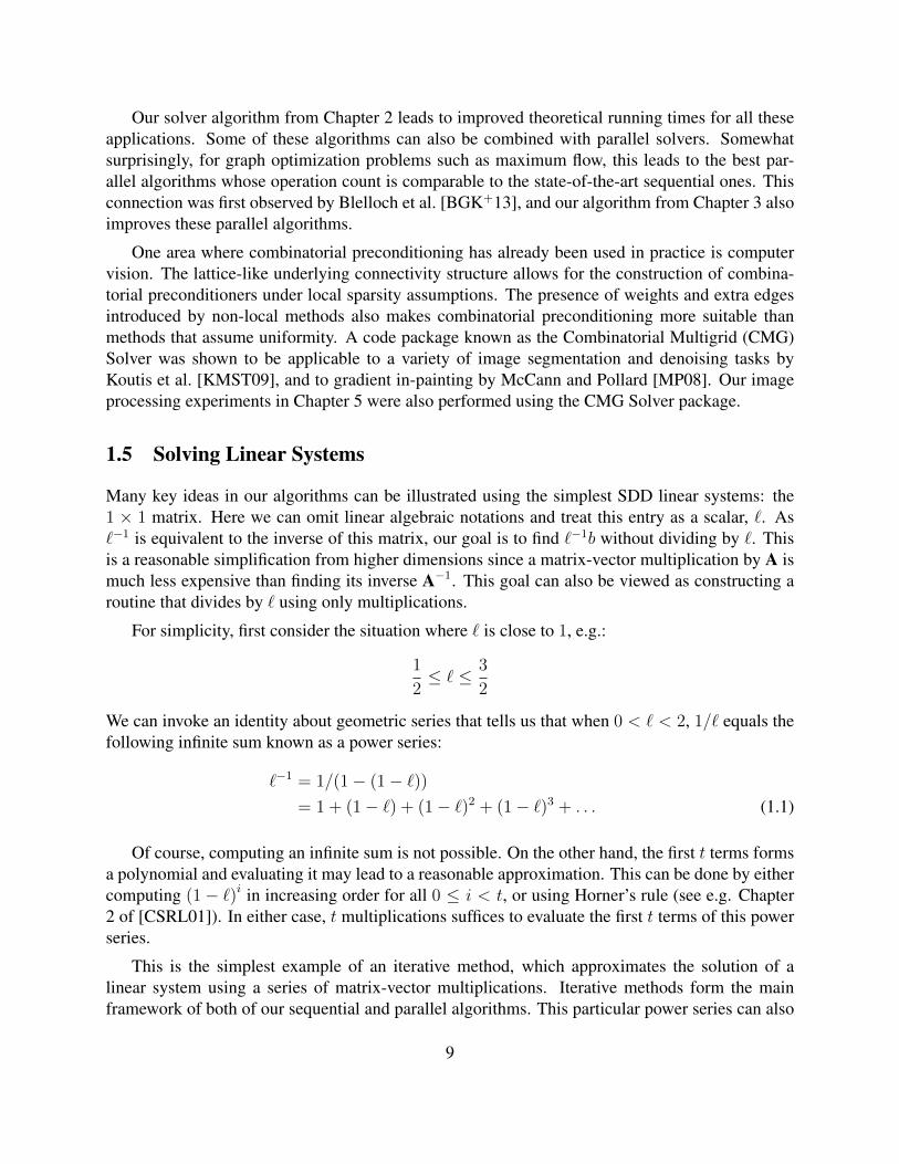
1.5 Solving Linear Systems
Many key ideas in our algorithms can be illustrated using the simplest SDD linear systems: the1 × 1 matrix. Here we can omit linear algebraic notations and treat this entry as a scalar, `. As`−1 is equivalent to the inverse of this matrix, our goal is to find `−1b without dividing by `. Thisis a reasonable simplification from higher dimensions since a matrix-vector multiplication by A ismuch less expensive than finding its inverse A−1. This goal can also be viewed as constructing aroutine that divides by ` using only multiplications.
For simplicity, first consider the situation where ` is close to 1, e.g.:
1
2≤ ` ≤ 3
2
We can invoke an identity about geometric series that tells us that when 0 < ` < 2, 1/` equals thefollowing infinite sum known as a power series:
`−1 = 1/(1− (1− `))= 1 + (1− `) + (1− `)2 + (1− `)3 + . . . (1.1)
Of course, computing an infinite sum is not possible. On the other hand, the first t terms formsa polynomial and evaluating it may lead to a reasonable approximation. This can be done by eithercomputing (1− `)i in increasing order for all 0 ≤ i < t, or using Horner’s rule (see e.g. Chapter2 of [CSRL01]). In either case, t multiplications suffices to evaluate the first t terms of this powerseries.
This is the simplest example of an iterative method, which approximates the solution of alinear system using a series of matrix-vector multiplications. Iterative methods form the mainframework of both of our sequential and parallel algorithms. This particular power series can also
9

be interpreted as computing the stationary distribution of a random walk, and we will explore thisconnection in more detail in Section 3.1.
The convergence of this type of method depends heavily on the value of 1 − `. The error ofusing the first t terms is given by the tail of infinite power series:
(1− `)t + (1− `)t+1 + (1− `)t+2 + . . . (1.2)
= (1− `)t(1 + (1− `)1 + (1− `)2 + . . .
)(1.3)
= (1− `)t `−1 (1.4)
If ` is in the range [1/2, 3/2], 1− ` is between [−1/2, 1/2] and (1− `)t approaches 0 geomet-rically. Therefore evaluating a small number of terms of the power series given in Equation 1.1leads to a good estimate. If we want an answer in the range [(1− ε) `−1b, (1 + ε) `−1b] for someerror ε > 0, it suffices to evaluate the first O (log (1/ε)) terms of this series.
On the other hand, convergence is not guaranteed when |1 − `| is larger than 1. Even if 1 − `is between (−1, 1), convergence may be very slow. For example, if ` is 1
κfor some large κ, the
definition of natural logarithm gives (1− `)κ ≈ 1e. That is, O(κ) steps are needed to decrease the
error of approximation by a constant factor.
Our two algorithms can be viewed as different approaches to accelerate this slow convergence.We first describe the approach taken for the sequential algorithm presented in Chapter 2, whichobtains an ε-approximation in O (m log n log (1/ε)) time.
1.5.1 Preconditioning
Preconditioning can be viewed as a systematic way to leverage the fact that some linear systems areeasier to solve than others. In our restricted setting of dividing by scalars, this may not be the casefor computers. However, it is certainly true for the reader: because our number system is base 10,it is much easier to divide a number by 0.1 (aka. multiply by 10). Consider the following situationwhere the recurrence given above converges slowly: ` is between 0.01 and 0.1. Since 1− ` can beas large as 0.99, about 100 iterations are needed to reduce the error by a constant factor. However,suppose instead of computing `x = b, we try to solve (10`)x = 10b. The guarantees on ` givesthat 10` is between 0.1 and 1, which in turn upper bounds 1 − ` by 0.9. This means 10 iterationsnow suffice to decrease the error by a constant factor, a tenfold speedup. This speedup comes at acost: we need to first multiply b by 10, and instead of computing 1−` we need to compute 1−10`.This results in an extra division by 0.1 at each step, but in our model of base ten arithmetic withscalars, it is much less expensive than most other operations.
The role that the value of 0.1 played is known as a preconditioner, and iterative methods in-volving such preconditioners are known as preconditioned iterative method. The recurrence thatwe showed earlier, unpreconditioned iterative methods, can be viewed as using the identity, 1 as apreconditioner. From this perspective, the reason for the tenfold speedup is apparent: for the rangeof ` that we are interested in, [0.01, 0.1], 0.1 is an estimate that’s better by a factor of ten whencompared to 1.
10

In general, because A is a matrix, the preconditioner which we denote as B also needs to be amatrix of the same dimension. As in the case with scalars, each step of a preconditioned iterativemethod needs to solve a linear system involving B. Also, the number of iterations depends on thequality of approximation of B to A. This leads to a pair of opposing goals for the construction of apreconditioner:
• B needs to be similar to A.
• It is easier to solve linear systems of the form Bx = b′.
To illustrate the trade-off between these two goals, it is helpful to consider the two extremepoints that completely meets one of these two requirements. If B = A, then the two matrices areidentical and only one iteration is required. However, solving a system in B is identical to solvinga system in A. On the other hand, using the identity matrix I as the preconditioner makes it veryeasy to solve, but the number of iterations may be large. Finding the right middle point betweenthese two conditions is a topic that’s central to numerical analysis (see e.g. [Axe94]).
Many existing methods for constructing preconditioners such as Jacobi iteration or Gauss-Seidel iteration builds the preconditioner directly from the matrix A. In the early 90s, Vaidyaproposed a paradigm shift [Vai91] for generating preconditioners:
Since A = LG corresponds to some graphG, its preconditionershould be the graph Laplacian of another graph H .
In other words, one way to generate a preconditioner for A is to generate a graph H basedon G, and let B = LH . Similarity between LG and LH can then be bounded using spectralgraph theory. This in turn allows one to draw connections to combinatorial graph theory and usemappings between the edges of G and H to derive bounds.
These ideas were improved by Boman and Hendrickson [BH01], and brought to full fruition inthe first nearly-linear time solver by Spielman and Teng [ST06]. Our sequential solver algorithmin Chapter 2 uses this framework with a few improvements. The main idea of this framework is tofind a graph H that’s similar to G, but is highly tree-like. This allows H to be reduced to a muchsmaller graph using a limited version of Gaussian elimination. More specifically, G and H arechosen so that:
• The preconditioned iterative method requires t iterations.
• The system that H reduces to is smaller by a factor of 2t.
This leads to a runtime recurrence of the following form:
T (m) = t(m+ T
(m2t
))(1.5)
11

Where the term of m inside the bracket comes from the cost of performing matrix-vector multipli-cations by A in each step, as well as the cost of reducing from H to the smaller system.
This runtime recurrence gives a total running time of O(mt). The call structure correspondingto this type of recursive calls is known in the numerical analysis as a W -cycle, as illustrated inFigure 1.3
m
m4
m4
m16
m16
m16
m16
Figure 1.3: Call structure of a 3-level W-cycle algorithm corresponding to the runtime recurrencegiven in Equation 1.5 with t = 2. Each level makes 2 calls in succession to a problem that’s 4times smaller.
Analyzing the graph approximations along with this call structure leads to the main result inChapter 2: a O(m log n log(1/ε)) time algorithm for computing answers within an approximationof 1± ε.
1.5.2 Factorization
Our parallel algorithm is based on a faster way of evaluating the series given in Equation 1.1. Aswe are solely concerned with this series, it is easier to denote 1− ` as α, by which the first t termsof this series simplifies to the following sum:
1 + α + α2 + . . . αt−1
Consider evaluating one term αi. It can be done using i multiplications involving α. However, ifi is a power of 2, e.g. i = 2k for some k, we can user much fewer multiplications since α2k is thesquare of α2k−1 . We can compute α2, α4, α8, . . . by repeatedly squaring the previous result, whichgives us α2k in k multiplications. It is a special case of the exponentiation by squaring (see e.g.Chapter 31 of [CSRL01]), which allows us to evaluate any αi in O(log i) multiplications.
This shortened evaluation suggest that it might be possible to evaluate the entire sum of thefirst t terms using a much smaller number of operations. This is indeed the case, and one way to
12

derive such a short form is to observe the result of multiplying 1 + α + . . . αt−1 by 1 + αt:(1 + αt
) (1 + α + . . . αt−1
)= 1 + α + . . .+ αt−1
+ αt + αt+1 . . . α2t−1
= 1 + α + . . .+ α2t−1
In a single multiplication, we are able to double the number of terms of the power series that weevaluate. An easy induction then gives that when t = 2k, the sum of the first t terms has a succinctrepresentation with k terms:
1 + α + . . . α2k−1 = (1 + α)(1 + α2
) (1 + α4
). . .(
1 + α2k−1)
This gives an approach for evaluating the first t terms of the series from Equation 1.1 inO(log t)matrix-vector multiplications. However, here our analogy between matrices and scalars breaksdown: the square of a sparse matrix may be very dense. Furthermore, directly computing the squareof a matrix requires matrix multiplication, for which the current best algorithm by Vassilevska-Williams [Wil12] takes about O(n2.3727) time.
Our algorithms in Chapter 3 give a way to replace these dense matrices with sparse ones. Wefirst show that solving any graph Laplacian can be reduced to solving a linear system I −A suchthat:
1. The power series given in Equation 1.1 converges to a constant error after a moderate (e.g.poly (n)) number of terms.
2. Each term in the factorized form of the power series involving A has a sparse equivalentwith small error.
3. The error caused by replacing these terms with their approximations accumulate in a con-trollable way.
The third requirement due to the fact that each step of the repeated squaring requires approx-imation. Our approximation of A4 is based on approximating the square of our approximation toA2. It is further complicated by the fact that matrices, unlike scalars, are non-commutative. Ouralgorithm handles these issues by a modified factorization that’s able to handle the errors incurredby successive matrix approximations. This leads to a slightly more complicated algebraic formthat doubles the number of matrix-vector multiplications. It multiplies by the matrix I + A bothbefore handing a vector off to routines involving the approximation to A2, and after receiving backan answer from it. An example of a call structure involving 3 levels is shown in Figure 1.4 . Whenviewed as a recursive algorithm, this is known as a V-cycle algorithm in the numerical analysisliterature.
One further complication arises due to the difference between scalars and matrices. The non-commutativity of approximation matrices with original ones means that additional steps are needed
13

to ensure symmetry of operators. When moving from terms involving A to A2, it performs matrix-vector multiplications involving I + A both before and after evaluating the problem involving A2
(or more accurately its approximation).
m
m
m
Figure 1.4: Call structure of a 3-level V-cycle algorithm. Each level makes 1 calls to a problem ofcomparable size. A small number of levels leads to a fast algorithm.
In terms of total number of operations performed, this algorithm is more expensive than theW-cycle algorithm shown in Chapter 2. However, a k-level V-cycle algorithm only has a O(k) se-quential dependency between the calls. As each call only performs matrix-vector multiplications,this algorithm is highly parallel. The V-cycle call structure is also present in the tool of choice usedin numerical analysis for solving SDD linear systems: multigrid algorithms (see e.g. [BHM00]).This connection suggests that further improvements in speed, or theoretical justifications for multi-grid algorithms for SDD linear systems may be possible.
1.6 Matrices and Similarity
The overview in Section 1.5 used the one-dimensional special case of scalars as illustrative exam-ples. Measuring similarity between n-dimensional matrices and vectors is more intricate. We needto bound the convergence of power series involving matrices similar to the one involving scalarsin Equation 1.1. Also, as we’re working with vectors with multiple entries, converging towards asolution vector also needs to be formalized. In this section we give some background on ways ofextending from scalars to matrices/vectors. All the results stated in this section are known toolsfor analyzing spectral approximations, and some of the proofs are deferred to Appendix A. Wewill distinguish between different types notationally as well: scalars will be denoted using regu-lar lower case characters, matrices by capitalized bold symbols, and vectors by bold lower casecharacters.
1.6.1 Spectral Decomposition
Spectral graph theory is partly named after the study of the spectral decomposition of the graphLaplacian LG. Such decompositions exist for any symmetric matrix A. It expresses A as a sum
14

of orthogonal matrices corresponding to its eigenspaces. These spaces are defined by eigen-value/vectors pairs, (λ1,u1) . . . (λn,un) such that Aui = λiui. Furthermore, we may assume thatthe vectors u1,u2 . . . un are orthonormal, that is:
uTi uj =
1 if i = j0 otherwise
The decomposition of A can then be written as:
A =n∑i=1
λiuiuTi
The orthogonality of the eigenspaces means that many functions involving A such as multipli-cation and inversion acts independently on the eigenspaces. When A is full rank, its inverse can bewritten as:
A−1 =n∑i=1
1
λiuiuTi
and when it’s not, this decomposition allows us to define the pseudoinverse. By rearranging theeigenvalues, we may assume that the only zero eigenvalues are λ1 . . . λn−r where r is the rank ofthe matrix (in case of the graph Laplacian of a connected graph, r = n− 1). The pseudoinverse isthen given by:
A† =n∑
i=n−r+1
1
λiuiuTi
This decomposition can also be extended to polynomials. Applying a polynomial p(x) =∑a0 +a1x
1 +a2x2 + . . .+adx
d to A leads to the matrix∑a0 +a1A +a2A2 + . . .+adAd. When
viewed using spectral decompositions, this matrix can also be viewed as applying the polynomialto each of the eigenvalues.
Lemma 1.6.1 If p(x) is a polynomial, then:
p(A) =n∑i=1
p(λi)uiuTi
Therefore, if p(λi) approaches 1λi
for all non-zero eigenvalues λi, then p(A) approaches A†
as well. This is the main motivation for the analogy to scalars given in Section 1.5. It meansthat polynomials that work well for scalars, such as Equation 1.1, can be used on matrices whoseeigenvalues satisfy the same condition.
15

1.6.2 Similarities Between Matrices and Algorithms
The way we treated p (A) as a matrix is a snapshot of a powerful way for analyzing numerical al-gorithms. It was introduced by Spielman and Teng [ST06] to analyze the recursive preconditioningframework. In general, many algorithms acting on b can be viewed as applying a series of lineartransformations to b. These transformations can in turn be viewed as matrix-vector multiplications,with each operation corresponding to a matrix. For example, adding the second entry of a length 2vector b to the first corresponds to evaluating:[
1 10 1
]b
and swapping the two entries of a length 2 vector b corresponds to evaluating:[0 11 0
]b
A sequence of these operations can in turn be written as multiplying b by a series of matrices.For example, swapping the two entries of b, then adding the second to the first can be written as:[
1 10 1
] [0 11 0
]b
In the absence of round-off errors, matrix products are associative. As a result, we may con-ceptually multiply these matrices together to a single matrix, which in turn represents our entirealgorithm. For example, the two above operations is equivalent to evaluating:[
1 11 0
]b
Most of our algorithms acting on an input b can be viewed as symmetric linear operators on b.Such operators can in turn be represented by (possibly dense) matrices, which we’ll denote using Zwith various subscripts. Even though such an algorithm may not explicitly compute Z, running itwith b as input has the same effect as computing Zb. This allows us to directly bound the spectralapproximation ratios between Z and A†.
Measuring the similarity between two linear operators represented as matrices is more com-plicated. The situation above with p (A) and A† is made simpler by the fact that their spectraldecompositions have the same eigenvectors. This additional structure is absent in most of ourmatrix-approximation bounds. However, if we are comparing A against the zero matrix, any spec-tral decomposition of A can also be used to give the zero matrix by setting all eigenvalues to 0.This gives a generalization of non-negativity to matrices known as positive semi-definiteness.
Definition 1.6.2 (Positive Semi-definiteness) A matrix A is positive semi-definite if all its eigen-values are non-negative.
16

This definition extends to pairs of matrices A,B in the same way as scalars. The matrix general-ization of ≤, , can be defined as follows:
Definition 1.6.3 (Partial Ordering Among Matrices) A partial ordering can be defined onmatrices by letting A B if B− A is positive semi-definite.
We can now formally state the guarantees of the power series given in Equation 1.1 when alleigenvalues of A are in a good range. The following proof is a simplified version of Richardsoniteration, more details on it can be found in Chapter 5.1. of [Axe94].
Lemma 1.6.4 If L is an n× n matrix with m non-zero entries where all eigenvalues are between12
and 32. Then for any ε > 0, there is an algorithm SOLVEL (b) that under exact arithmetic is a
symmetric linear operator in b and runs inO (m log (1/ε)) time. The matrix realizing this operator,Z, satisfies:
(1− ε) L† Z (1 + ε) L†
Proof Our algorithm is to evaluate the first N = O (log (1/ε)) terms of the power series fromEquation 1.1. If we denote this polynomial as pN , then we have Z = pN (L). Its running timefollows from Horner’s rule (see e.g. Chapter 2 of [CSRL01]) and the cost of making one matrix-vector multiplication in I− L.
We now show that Z spectrally approximates L†. Let a spectral decomposition of L be:
L =n∑i=1
λiuiuTi
Lemma 1.6.1 gives that applying pN to each eigenvalue also gives a spectral decomposition to Z:
Z =n∑i=1
pn (λi) uiuTi
Furthermore, the calculations that we performed in Section 1.5, specifically Equation 1.4 gives thatpn (λi) is a 1± ε approximation to 1
λi:
(1− ε) 1
λi≤ pn (λi) ≤ (1 + ε)
1
λi
This in turn implies the upper bound on Z:
(1 + ε) L† − Z =n∑i=1
(1 + ε)1
λiuiuTi −
n∑i=1
pN (λi) uiuTi
=n∑i=1
((1 + ε)
1
λi− pN (λi)
)uiuTi
17

This is a spectral decomposition of (1 + ε) L† − Z with all eigenvalues non-negative, thereforeZ (1 + ε) L†. The LHS also follows similarity.
Showing bounds of this form is our primary method of proving convergence of algorithms inthis thesis. Most of our analyses are simpler than the above proof as they invoke known resultson iterative methods as black-boxes. Proofs of these results on iterative methods are given inAppendix D for completeness. The manipulations involving that we make mostly rely on factsthat extends readily from scalars. We will make repeated use of the following two facts in ouralgebraic manipulations.
Fact 1.6.5 If A, B are n× n positive semi-definite matrices such that A B, then:
1. For any scalar α ≥ 0, αA αB.
2. If A′ and B′ are also n× n positive semi-definite matrices such that A′ B′, then A + A′ B + B′.
The composition of under multiplication is more delicate. Unlike scalars, A B and Vbeing positive semi-definite do not imply AV BV. Instead, we will only use compositionsinvolving multiplications by matrices on both sides as follows:
Lemma 1.6.6 (Composition of Spectral Ordering) For any matrices V,A,B, if A B, thenVTAV VTBV
1.6.3 Error in Vectors
Viewing algorithms as linear operators and analyzing the corresponding matrices relies cruciallyon the associativity of the operations performed. This property does not hold under round-offerrors: multiplying x by y and then dividing by y may result in an answer that’s different thanx. As a result, guarantees for numerical algorithms are often more commonly stated in terms ofthe distance between the output and the exact answer. Our main results stated in Section 1.3 arealso in this form. Below we will formalize these measures of distance, and state the their closeconnections to the operator approximations mentioned above.
One of the simplest ways of measuring the distance between two vectors x and x is by theirEuclidean distance. Since distances are measured based on the difference between x and x, x− x,we may assume x = 0 without loss of generality. The Euclidean norm of x is
√xTx, and can also
be written as√
xT Ix where I is the identity matrix. Replacing this matrix by A leads to matrixnorms, which equals to xTAx.
Matrix norms are useful partly because they measure distances in ways aligned to the eigenspacesof A. Replacing A by its spectral decomposition A gives:
xTAx =∑i
λixTuTi uix
=∑i
λi(xTu
)2
18

When λi ≥ 0, this is analogous to the Euclidean norm with different weights on entries. Therefore,positive semi-definite matrices such as SDD matrices leads to matrix norms. The A-norm distancebetween two vectors x and y can then be written as:
‖x− x‖A =
√(x− x)T A (x− x)
When A is positive semi-definite, the guarantees for algorithms for solving linear systems in Aare often stated in terms of the A-norm distance between x and x. We can show that the operatorbased guarantees described above in Section 1.6.2 is a stronger condition than small distances inthe A-norm.
Lemma 1.6.7 If A is a symmetric positive semi-definite matrix and B is a matrix such that:
(1− ε) A† B (1 + ε) A†
then for any vector b = Ax, x = Bb satisfies:
‖x− x‖A ≤ ε ‖x‖A
We can also show that any solver algorithm with error < 1 can be improved into a 1± ε one byiterating on it a small number of times. A variant of Richardson iteration similar to the one used inthe proof of Lemma 1.6.4 leads to the following black-box reduction to constant factor error:
Lemma 1.6.8 If A is a positive semi-definite matrix and SOLVEA is a routine such that for anyvector b = Ax, SOLVEA (b) returns a vector x such that:
‖x− x‖A ≤1
2‖x‖A
Then for any ε, there is an algorithm SOLVE′A such that any vector b = Ax, SOLVE′A (b) returns avector x such that:
‖x− x‖A ≤ ε ‖x‖A
by making O (log (1/ε)) calls to SOLVE′A and matrix-vector multiplications to A. Furthermore,SOLVE′A is stable under round-off errors.
This means that obtaining an algorithm whose corresponding linear operator is a constant factorapproximation to the inverse suffices for a highly efficient solver. This is our main approach foranalyzing the convergence of solver algorithms in Chapters 2 and 3.
1.6.4 Graph Similarity
The running times and guarantees of our algorithms rely on bounds on spectral similarities betweenmatrices. There are several ways of generating spectrally close graphs, and a survey of them can
19

be found in an article by Batson et al. [BSST13]. The conceptually simplest algorithm for spectralsparsification is by Spielman and Srivastava [SS08]. This algorithm follows the sampling schemeshown in Algorithm 1, which was first introduced in the construction of cut sparsifiers by Benczurand Karger [BK96]
Algorithm 1 Graph Sampling Scheme
SAMPLE
Input: Graph G = (V,E,w), non-negative weight τ e for each edge, error parameter ε.Output: Graph H ′ = (V,E ′,w′).
1: for O(∑
τ log nε−2) iterations do2: Pick an edge with probability proportional to its weight3: Add a rescaled copy of the edge to the sampled graph4: end for
This algorithm can be viewed as picking a number of edges from a distribution. These samplesare rescaled so that in expectation we obtain the same graph. Spielman and Srivastava [SS08]showed the that for spectral approximations, the right probability to sample edges is weight timeseffective resistance. Recall that the effective resistance of an edge e = uv is the voltage needed topass 1 unit of current from u to v. Formally the product of weight and effective resistance, τe canbe defined as:
τ e = wuvχTuvL
†Gχuv (1.6)
Where L†G is the pseudo-inverse of LG and χuv is the vector with −1 at vertex u and 1 at vertexv. It was shown in [SS08] that if τ are set close to τ , the resulting graph H is a sparsifier for Gwith constant probability. This proof relied on matrix-Chernoff bounds shown independently byRudelson and Vershynin [RV07], Ahlswede and Winter [AW02], and improved by Tropp [Tro12].Such bounds also play crucial roles in randomized numerical linear algebra algorithms, where thevalues τe described above are known as statistical leverage scores [Mah11].
Koutis et al. [KMP10] observed that if τ upper bounds τ entry-wise, H will still be a spar-sifier. Subsequent improvements and simplifications of the proof have also been made by Ver-shynin [Ver09] and Harvey [Har11]. To our knowledge, the strongest guarantees on this samplingprocess in the graph setting is due to Kelner and Levin [KL11] and can be stated as follows:
Theorem 1.6.9 For any constant c, there exist a setting of constants in the sampling scheme shownin Algorithm 1 such that for any weighted graph G = (V,E,w), upper bounds τ ≥ τ , anderror parameter ε, the graph H given by the sampling process has O (
∑e τ e log nε−2) edges and
satisfies:
(1− ε)LG LH (1 + ε)LG
with probability at least 1− n−c
20

A proof of this theorem, as well as extensions that simplify the presentation in Chapter 2 aregiven in Appendix B. The (low) failure rate of this algorithm and its variants makes most of oursolver algorithms probabilistic. In general, we will refer to a success probability of 1 − n−c forarbitrary c as “high probability”. As most of our algorithms rely on such sampling routines, wewill often state with high probability instead of bounding probabilities explicitly.
A key consequences of this sparsification algorithm can be obtained by combining it withFoster’s theorem [Fos53].
Lemma 1.6.10 For any graph, the sum of weight times effective resistance over all edges is exactlyn− 1,
∑e τ e = n− 1.
Combining Lemma 1.6.10 with Theorem 1.6.9 gives that for any graph G and any ε > 0,there exists a graph H with O (n log nε−2) edges such that (1 − ε)LG LH (1 + ε)LG. Inother words, any dense graph has a sparse spectral equivalent. Obtained spectrally similar graphsusing upper bounds of these probabilities is a key part of our algorithms in Chapters 2 and 3. Theneed to compute such upper bounds is also the main motivation for the embedding algorithms inChapter 4.
21

22

Chapter 2
Nearly O(m log n) Time Solver
In this chapter we present sequential algorithms for solving SDD linear systems based on combi-natorial preconditioning. Our algorithms can be viewed as both a speedup and simplification ofthe algorithm by Spielman and Teng [ST06]. One of the key insights in this framework is thatfinding similar graphs with fewer edges alone is sufficient for a fast algorithm. Specifically, if thenumber of edges is n plus a lower order term, then the graph is ‘tree like’. Repeatedly performingsimple reduction steps along the tree reduces the graph to one whose size is proportional to thenumber of off-tree edges. This need for edge reduction will also be the main driving goal behindour presentation.
We will formalize the use of these smaller graphs, known as ultra-sparsifiers in Section 2.1, thendescribe our algorithms in the rest of this chapter. To simplify presentation, we first present theguarantees of our algorithm in the model where all arithmetic operations are exact. The numericalstability of the algorithm is then analyzed in the fixed point arithmetic model in Section 2.6. Themain components of these algorithms appeared in two papers joint with Ioannis Koutis and GaryMiller [KMP10, KMP11], while the improvements in Section 2.5 is joint with Gary Miller andunpublished. Our result in the strongest form is as follows:
Theorem 2.0.1 Let L be an n × n graph Laplacian with m non-zero entries. We can preprocessL in O (m log n log log n) time so that, with high probability, for any vector b = Lx, we can findin O (m log n log(1/ε)) time a vector x satisfying ‖x− x‖L < ε ‖x‖L. Furthermore, if fixed pointarithmetic is used with the input given in unit lengthed words, O(1) sized words suffices for the theoutput as well as all intermediate calculations.
When combined with the nearly-optimal construction of ultra-sparsifiers by Kolla et al. [KMST10],our approach in Section 2.5 also implies solver algorithms that runs inO
(m√
log n log (1/ε))
timefor any vector b. We omit this extension as it requires quadratic preprocessing time using existingtechniques.
2.1 Reductions in Graph Size
Our starting point is an iterative method with improved parameters. Given graphs G and H and aparameter κ such that LG LH κLG, a recurrence similar to Equation 1.1 allows us to solve a
23

linear system involving LG to constant accuracy by solvingO(κ) ones involving LH . This iterationcount can be improved using Chebyshev iteration to O (
√κ). Like Richardson iteration, it is well-
known in the numerical analysis literature [Saa03, Axe94]. The guarantees of Chebyshev iterationunder exact arithmetic can be stated as:
Lemma 2.1.1 (Preconditioned Chebyshev Iteration) There exists an algorithm PRECONCHEBY
such that for any symmetric positive semi-definite matrices A, B, and κ where
A B κA
any error tolerance 0 < ε ≤ 1/2, PRECONCHEBY(A,B, b, ε) in the exact arithmetic model is asymmetric linear operator on b such that:
1. If Z is the matrix realizing this operator, then (1− ε)A† Z (1 + ε)A†
2. For any vector b, PRECONCHEBY(A,B, b, ε) takes N = O (√κ log (1/ε)) iterations, each
consisting of a matrix-vector multiplication by A, a solve involving B, and a constant numberof vector operations.
A proof of this Lemma is given in Appendix D.2 for completeness. Preconditioned Chebysheviteration will serve as the main driver of the algorithms in this chapter. It allows us to transform thegraph into a similar one which is sparse enough to be reduced by combinatorial transformations.
These transformations are equivalent to performing Gaussian elimination on vertices of degrees1 and 2. In these limited settings however, this process has natural combinatorial interpretations.We begin by describing a notion of reducibility that’s a combinatorial interpretations of partialCholesky factorization. This interpretation is necessary for some of the more intricate analysesinvolving multiple elimination steps.
Definition 2.1.2 A graph G with mG edges is reducible to a graph H with mH edges if given anysolver algorithm SOLVEH corresponding to a symmetric linear operator on b such that:
• For any vector b, SOLVEH (b) runs in time T
• The matrix realizing this linear operator, ZH satisfies: L†H ZH κL†H
We can create in O(1) time a solver algorithm for LG, SOLVEG that is a symmetric linear operatoron b such that:
• For any vector b, SOLVEG (b) runs in time T +O (mG −mH)
• The matrix realizing this linear operator, ZG satisfies: L†G ZG κL†G
We will reduce graphs using the two rules below. They follow from standard analyses of partialCholesky factorization, and are proven in Appendix C for completeness.
24

Lemma 2.1.3 LetG be a graph where vertex u has only one neighbor v. H is reducible to a graphH that’s the same as G with vertex u and edge uv removed.
Lemma 2.1.4 Let G be a graph where vertex u has only two neighbors v1, v2 with edge weightswuv1 and wuv2 respectively. G is reducible a graph H that’s the same as G except with vertex uand edges uv1, uv2 removed and weight
wuv1wuv2
wuv1 + wuv2
=1
1wuv1
+ 1wuv2
added to the edge between v1 and v2.
These two reduction steps can be applied exhaustively at a cost proportional to the size reduc-tion. However, to simplify presentation, we will perform these reductions only along a (spanning)tree. It leads to a guarantee similar to the more aggressive version: applying these tree reductionsgreedily on graph with n vertices and m edges results in one with O(m − n) vertices and edges.We will term this routine GREEDYELIMINATION.
Lemma 2.1.5 (Greedy Elimination) Given a graph G along with a spanning tree TG, there is aroutine GREEDYELIMINATION that performs the two elimination steps in Lemmas 2.1.3 and 2.1.4on vertices that are incident to no off-tree edges and have degree at most 2. If G has n verticesand m edges, GREEDYELIMINATION(G, TG) returns in O(m) time a graph H containing at most7(m − n) vertices and edges along such that G is reducible to H , along with a spanning tree THof H formed by
Proof Note that each of the two operations affect a constant number of vertices, and removes thecorresponding low degree vertex. Therefore, one way to implement this algorithm in O(m) timeis to track the degrees of tree nodes, and maintain an event queue of low degree vertices.
We now bound the size of H . Let the number of off-tree edges be m′, and V ′ be the set ofvertices incident to some off tree edge, then |V ′| ≤ 2m′. The fact that none of the operations canbe applied means that all vertices in V (H) \ V ′ have degree at least 3. So the number of edges inH is at least:
3
2(nh − |V ′|) +m′
On the other hand, both the two reduction operations in Lemmas 2.1.3 and 2.1.4 preserves the factthat T is a tree. So there can be at most nH − 1 tree edges in H , which means the total number ofedges is at most:
nH − 1 +m′ ≤ nH +m′
25

Combining these two bounds gives:
3
2(nH − |V ′|) +m′ ≤ nH +m′
3nH − 3|V ′| ≤ 2nH
nH ≤ 3|V ′| ≤ 6m′
Since the tree in H has nH − 1 edges, the number of edges can in turn be bounded by nH +m′ ≤7m′.
Therefore significant savings in running times can be obtained if G is tree-like. This motivatedthe definition of ultra-sparsifiers, which are central to the solver framework by Spielman and Teng[ST06]. The following is equivalent to Definition 1.1 of [ST06], but is graph theoretic and makesthe tree-like structure more explicit.
Definition 2.1.6 (Ultra-Sparsifiers) Given a graphG with n vertices andm edges, a (κ, h)-ultra-sparsifier H is a graph on the same set of vertices such that:
• H consists of a spanning tree T along with hmκ
off-tree edges.
• LG LH κLG.
Spielman and Teng showed that fast algorithms for constructing (κ, h)-ultra-sparsifiers leadsto solvers for SDD linear systems that run in O (mh log (1/ε)) time. At a high level this is becauseLemma 2.1.5 allows us to reduce solving a linear system on the ultra-sparsifier to one on a graphof size O(hm
κ) edges, while Lemma 2.6.3 puts the iteration count at κ. So the running time for
solving a system with m edges, T (m) follows a recurrence of the form:
T (m) ≤ O(√
κ)(
m+ T(hm
κ
))Which is optimized by setting κ to about h2, and solves to T (m) = O (hm).
We will first show a construction of (κ,O(log2 n))-ultra-sparsifiers in Section 2.2, which bythemselves imply a solver that runs in about m5/4 time. In Section 2.3, we describe the recursivepreconditioner framework from [ST06] and show that it leads to a O(m log2 n log log n log(1/ε))time solver. Then we optimize this framework together with our ultra-sparsification algorithm toshow an even faster algorithm in Section 2.5. This gives an algorithm for solving graph Laplaciansin O(m log n log(1/ε)) time.
2.2 Ultra-Sparsification Algorithm
As with the case of generating spectral sparsifiers, sampling by (upper bounds of) effective re-sistance is also a natural approach for generating ultra-sparsifiers. However, to date obtaininghigh quality estimates of effective resistances in nearly-linear time without using solvers remains
26

an open problem. Our workaround to computing exact effective resistances relies on Rayleigh’smonotonicity law.
Lemma 2.2.1 (Rayleigh’s Monotonicity Law) The effective resistance between two vertices doesnot decrease when we remove edges from a graph.
This fact has a simple algebraic proof by the inequality (LG + LG′)† L†G as long as the
null space on both sides are the same. It’s also easy to check it in the extreme case. When edgesare removed so that two vertices are disconnected, the effective resistance between them becomesinfinite, which is at least any previous values.
Our use of Rayleigh’s monotonicity law will avoid extreme case, but just barely. We remove asmany edges as possible while keeping the graph connected. In other words, we will use resistivevalues w.r.t. a single tree as upper bounds for the true effective resistance τe. Since there is onlyone path connecting the end points of e in the tree, the resistance between its two end points is thesum of the resistive values along this path.
An example of this calculation is shown in Figure2.1, where the tree that we calculate theresistive value by is shown in bold.
4
52
2
Figure 2.1: The effective resistance RT (e) of the blue off-tree edge in the red tree is 1/4 + 1/5 +1/2 = 0.95. Its stretch strT (e) = weRT (e) is (1/4 + 1/5 + 1/2)/(1/2) = 1.9
An edge’s weight times its effective resistance measured according to some tree can also bedefined as its stretch 1. This is a central notion in metric embedding literature [AKPW95] and hasbeen extensively studied [Bar96, Bar98, FRT04, EEST08, ABN08, AN12]. As a result, we will usestrT (e) as an alternate notation for this product of weight and tree effective resistance. Formally,if the path between the end points of e is PT (e), the stretch of edge e is:
strT (e) =we
∑e′∈PT (e)
re′
=we
∑e′∈PT (e)
1
we′(2.1)
We can also extend this notation to sets of edges, and use strT (EG) to denote this total stretch ofall edges in G. Since stretches are upper bounds for sampling probabilities, the guarantees of thesampling procedure from Theorem 1.6.9 can be stated as:
1Formally, it equals to stretch in the graph where the length of an edge is the reciprocal of its weight. We willformalize this in Chapter 4
27

Lemma 2.2.2 There is an algorithm that takes a graph G = (V,EG,w) with n vertices and aspanning tree and returns a graph H with n − 1 + O (strT (EG \ ET ) log n) edges such that withhigh probability:
1
2LG LH
3
2LG
Note that the number of off-tree edges retained equals to O(log n) times their total stretch,strT (EG \ ET ). As the stretch of an edge corresponds to the probability of it being sampled,we need a tree where the total stretch to be as low as possible. Due to similar applications ofa tree with small total stretch in [ST06], algorithms generating them have received significantinterest [EEST08, ABN08, KMP11, AN12]. The current state of the art result is by Abraham andNeiman [AN12]:
Theorem 2.2.3 There is an algorithm LOWSTRETCHTREE such that given a graphG = (V,E,w′),LOWSTRETCHTREEG outputs a spanning tree T of G satisfying
∑e∈E = O(m log n log log n) in
O(m log n log log n) time.
Combining Lemma 2.2.2 and Theorem 2.2.3 as stated gives H with O(m log2 n log log n)edges, which is more edges than the number of edges in G. Of course, these ‘extra’ edges ex-ist in the form of multi-edges, and the edge count in the resulting graph can still be bounded by m.One way to see why direct sampling by stretch is not fruitful is to consider the case where all edgesin the graph have unit weight (and therefore unit resistance). Here the stretch of an edge cannotbe less than 1, which means the total estimates that we get is at least m. When combined with theguarantees of the Sampling algorithm from Theorem 1.6.9, this leads to more edges (samples to beprecise) than we started with.
We remedy this issue by bringing in the parameter that we have yet to use: κ. Note that so far,the sparsifiers that we generated are off only by a constant factor from G, while the definition ofultra-sparsifiers allow for a difference of up to κ. We will incorporate this parameter in the simplestway possible: scale up the tree by a factor of κ and applying this sampling algorithm. This leadsto the algorithm shown in Algorithm 2. The guarantees of this algorithm is as follows:
Algorithm 2 Ultra-sparsification Algorithm
ULTRASPARSIFY
Input: Graph G, spanning tree T , approximation factor κOutput: Graph H
1: Let G′ be G with T scaled up by a factor of κ, and T ′ the scaled up version of T2: Calculate τ e = min1, strT ′(e) for all e /∈ T ′3: return T ′ + SAMPLE(EG′ \ ET ′ , τ )
28

Theorem 2.2.4 (Ultra-Sparsifier Construction) There exists a setting of constants in ULTRA-SPARSIFY such that given a graph G and a spanning tree T , ULTRASPARSIFY(G, T) returns inO(m log n + strT (G) log2 n
κ) time a graph H that is with high probability a
(κ,O
(strT (G)m
log n))
-ultra-sparsifier for G.
Proof Let G′ be the graph G with T scaled up by a factor of κ. We first bound the conditionnumber. Since the weight of an edge is increased by at most a factor of κ, we have G G′ κG.
Furthermore, because of the scaling, the effective resistance along the tree of each non-treeedge decreased by a factor of κ. Thus for any off tree edge e, we have:
strT ′(e) =1
κstrT (e)
Summing over all edges gives:
strT ′(EG′ \ ET ′) ≤1
κstrT (EG \ ET )
Using Lemma 2.2.2, we can obtain a graphH with n vertices and n−1+ 1κO (strT (EG \ ET ) log n)
edges such that with high probability:
1
2LG′ LH
3
2LG′
Chaining this with the relation between G and G′ gives:
LG LG′ 2LH 3LG′ 3κLG
For the running time, we need to first computed the effective resistance of each non-tree edgeby the tree. This can be done using the offline LCA algorithm [Tar79], which takes O (mα (m)) inthe pointer machine model. This is less than the first term in our bound. To perform each step ofthe sampling process, we map each edge to an interval of [0, 1], and find the corresponding samplein O(log n) time via. binary search. This gives the second term in our bound.
Using this ultra-sparsification algorithm with κ = m1/2 log2 n log log n leads to a solver algo-rithm that runs in about m5/4 time.
Lemma 2.2.5 In the exact floating arithmetic model, given a graph Laplacian for G with n ver-tices and m edges, we can preprocess G in O (m log n log log n) time to obtain a solver algorithmSOLVEG that’s a symmetric linear operator on b such that with high probability:
• For any vector b, SOLVEG (b) runs in O(m5/4 log n
√log log n
)time.
• If Z is a matrix realizing this operator, we have: 12L†G Z 3
2L†G
29

Proof Consider the following two-level scheme: generate a (κ, h)-ultra-sparsifierH using Lemma 2.2.4,reduce its size using the greedy elimination procedure given in Lemma 2.1.5 to obtain G1, andcompute an exact inverse of the smaller system.
SinceH has n vertices and n−1+hmk
edges, the greedy elimination procedure from Lemma 2.1.5
gives that G1 has size O(hmk
) vertices and edges. Therefore, the inverse of G1 has size O((
hmk
)2)
and can be computed using matrix inversion in O((
hmk
)ω) time [Wil12].
Also, the condition number of κ implies that O(√κ) iterations are needed to obtain a solver for
LG. Each iteration consists of a matrix-vector multiplication involving LG, and a solve involvingLH . This gives a total running time of:
O
(√κ
(m+
(hm
κ
)2)
+
(hm
κ
)ω)(2.2)
The inner term is optimized when κ = h√m, giving a total running time of:
O(h
12m
54 log(1/ε) +m
ω2
)(2.3)
The current best bound of ω ≈ 2.37 [Wil12] gives ω2< 5
4, so the last term can be discarded.
Substituting in h = O(log2 n log log n) gives the stated running time.
2.3 Recursive Preconditioning and Nearly-Linear Time Solvers
As alluded at the end of Section 2.1, the full potential of ultra-sparsifiers are realized when they areapplied in a recursive fashion. A main technical issue that needs to be resolved is that each levelof the recursion produces an approximate solution. This means that errors need to be propagatedup the levels of the recursion. As a result, it’s useful to list the systems involved in all layers of therecursive calls in the form of G0 . . . Gd. To construct level i + 1 of this chain, we first construct a(κi, h)-ultra-sparsifier for Gi, Hi+1. Then Gi+1 is obtained by performing greedy elimination onHi+1. This structure can be formalized via. the definition of a preconditioner chain.
Definition 2.3.1 (Preconditioning Chain) A preconditoining chain for a graph G is a sequenceof graphs G = G0, H1, G1, . . . , Gd along with size bounds m0,m1, . . . ,md and spectralbounds κ0, κ1, . . . , κd such that:
1. LGi LHi+1 κiLGi for all 0 ≤ i ≤ d− 1 and κd = 1.
2. Gi = GREEDYELIMINATION(Hi) for all i ≥ 1.
3. The size of Gi is at most mi and md is smaller than a fixed constant.
The extra condition of κd = 1 is to ease the runtime analysis, since the number of matrix-vector multiplies involving Gi also depends on κi. The preconditioning chain leads to recursive
30

algorithms for solving linear systems involving Gi. Preconditioned Chebyshev iteration allows usto solve this system by making O(
√κi) calls to solves involving Hi. This in turn leads to solves
involving Gi+1. This leads to the W-cycle algorithm described in Section 1.5.1. Its performancecan be described using the parameters of the preconditioning chain as follows:
Lemma 2.3.2 Given a preconditioning chain along with any error parameter ε, for each i there isan algorithm SOLVEGi such that:
• For any vector b, SOLVEGi (b) runs in time: O(∑d
i′=imi′∏i′
j=i
√crecκj
), where crec is an
absolute constant.
• SOLVEGi corresponds to a symmetric linear operator on b, and if ZGi is the matrix realizingthis operator, it satisfies: 1
2L†Gi ZGi 3
2L†Gi
Proof The proof is by induction backwards on the levels i. The case where i = d follows by theassumption that md is smaller than a constant. Suppose the result is true for i + 1, then we havean algorithm SOLVEGi+1
that’s a symmetric linear operator and its corresponding matrix ZGi+1
satisfies:
1
2L†Gi+1
ZGi+1 3
2L†Gi+1
As Gi+1 was obtained by greedy elimination from Hi+1, Hi+1 is reducible to Gi+1. Therefore wecan obtain an algorithm SOLVEHi+1
corresponding to a matrix ZHi+1such that:
1
2L†Hi+1
ZHi+1 3
2L†Hi+1
2
3LHi+1
Z†Hi+1 2LHi+1
The definition of reducibility in Defintion 2.1.2 gives that computing ZHi+1b for some vector b
takes time that’s O(mi −mi+1) = O(mi) more than the time of running SOLVEHi+1. Invoking the
inductive hypothesis gives that SOLVEHi+1runs in time:
O (mi) +d∑
i′=i+1
mi′
i′∏j=i+1
√crecκj ≤ O(mi) +
d∑i′=i+1
mi′
i′∏j=i+1
√crecκj
As LHi+1satisfies LGi LHi+1
κiLGi , Z†Hi+1also satisfies:
2
3LGi Z†Hi+1
2κiLGi
Therefore preconditioned Chebyshev iterations as given by Lemma 2.1.1 with A = LGi andB = 3
2Z†Hi+1
gives us a routine SOLVEGi meeting the required conditions. Its iteration count is
31

O(√
23κi) = O(
√κi). Furthermore, each solve involving B is equivalent to computing 2
3ZHi+1
b′
for some vector b′. This is in turn equivalent to calling SOLVELHi+1(b′). Substituting the running
time this routine gives a total running time of:
O (√κi)
(O(mi) +
d∑i′=i+1
mi′
i′∏j=i+1
√crecκj
)
= miO(√κi) +O(
√κi) ·
d∑i′=i+1
mi′
i′∏j=i+1
√crecκj
By choosing crec to be larger than the absolute constants and rearranging gives the total runtime.
This recursive framework was envisioned with ultra-sparsifiers in mind. Therefore, our ultra-sparsification algorithm from Theorem 2.2.4 can readily substituted into it. By picking a uniformκ at each level and rerunning the ultra-sparsification algorithm, we obtain the following result firstshown in [KMP10].
Lemma 2.3.3 In the exact arithmetic model, given a graph G with n vertices, m edges, and cor-responding graph Laplacian LG. For any vector b = LGx and and error ε > 0, we can find inO(m log2 n log log n log(1/ε)) time a vector x such that with high probability:
‖x− x‖A ≤ ε ‖x‖A
Algorithm 3 Simple Preconditioning Chain Construction
BUILDCHAINSIMPLE
Input: Graph G.Output: Preconditioning chain.
1: G0 := G2: d = 03: Pick appropriate constants c and cstop.4: while md > cstop do5: TGd ← LOWSTRETCHTREE(Gd)6: κd ← c log4 nd log log2 nd7: Hd+1 ← ULTRASPARSIFY(Gd, TGd , κd)8: Gd+1 ← GREEDYELIMINATION(Hd+1)9: d← d+ 1
10: end while11: return G0, H1, G1, . . . Hd, Gd, κ0 . . . κd−1, 1
Proof We will generate a preconditioning chain by calling the ultra-sparsifier on Gi and per-forming greedy elimination until Gi is of constant size. Pseudocode of this algorithm is shown
32

in Algorithm 3. Since we only made O(log n) calls to ULTRASPARSIFY, applying union boundgives that these calls all succeed with high probability. If we let cu be the constant from theultra-sparsification algorithm from Theorem 2.2.4 and the low-stretch spanning tree from Theo-rem 2.2.3, the the number of off-tree edges in Hi can be bounded by:
cu log2mi log logmi
c log4mi log log2mi
mi =cu
c log2mi log logmi
mi
Since Gi+1 is obtained from Hi+1 using greedy elimination, its edge count can be bounded usingLemma 2.1.5:
mi+1 ≤7cu
c log2mi log logmi
mi
Applying this inductively gives;
mi ≤ m0
i−1∏j=0
(7cu
c1 log2 nj log log nj
)Recall that the total work for SOLVE(G0) given by Lemma 2.3.2 is:
d∑i=0
mi
i∏j=0
√crecκj
Invoking the bound on mi on each term allows us to bound them as:
mi
i∏j=i
√crecκj ≤ m0
i−1∏j=0
(7cu
c log2 nj log log nj
) i∏j=0
√crecκj
≤ m0
i−1∏j=0
(7cu
c log2 nj log log nj
) i∏j=0
√crecc log4 nj log log2 nj
= m0
√crecc log4 ni log log2 ni
i−1∏j=0
7cu
√crecc log4 nj log log2 nj
c log2 nj log log nj
= m0
√crecc log4 ni log log2 ni
i−1∏j=0
(7cu√crec√c
)
So if we pick c such that c ≥ 100c2ucrec, the last term can be bounded by
(12
)i Also, since c and crecare both constants and ni ≤ n, the first term can be bounded by O(log2 n log log n). So the overall
33

work can be bounded by:
d∑i=0
O(m log2 n log log n)
(1
2
)iAs the terms are geometrically decreasing, this gives a total of O(m log2 n log log n). The runtimeneeded to get to an accuracy of ε can then be obtained by converting error to vector form as shownin Lemma 1.6.7, and reducing error by iterating using Lemma 1.6.8
2.4 Reuse, Recycle, and Reduce the Tree
We now show that a more holistic examination of the preconditioning chain leads to an evenfaster algorithm. The key observation is that the previous low stretch spanning tree remains asan extremely good tree in the ultrasparsifier. Here it is helpful to view both ULTRASPARSIFY andGREEDYELIMINATION as returning a tree along with a graph. We first observe that if (H,TH) isreturned by ULTRASPARSIFY(G, TG, κ), the total stretch of H w.r.t TH is smaller by a factor of κ,aka. strTG(G)/κ.
Lemma 2.4.1 If (H,TH) = TREEULTRASPARSIFY(G, TG, κ), then strTH (H) = strTG(G)/κ
Proof Let G′i be the graph formed by scaling up TG by a factor of κ in G. Let the new tree in thisgraph be T ′G. By definition of stretch we have strTG′ (G
′) = strTG(G)/κ.
Now consider the effect of the sampling procedure used to obtain H from G′. Clearly the treeis unchanged, TH = TG′ . When an edge e is picked, its weight is rescaled to its weight divided bythe probability of it being sampled, which is in turn proportional to its stretch times log n. So thenew weight is:
w′e =we
pe
=we
strTH (e)cs log n
=we
weRTH (e)cs log n
=1
RTH (e)cs log n
So the stretch of the edge when sampled is:
strTH (e′) = w′eRTH (e)
=1
cs log n
34
As the total number of edges sampled is csstrTH (G′) log n = cs log nstrTG (G)
κ, we have strTH (H) =
strTG (G)
κ.
The other operation that we perform on the graphs is GREEDYELIMINATION. We next showthat it also does not increase the total stretch of the off-tree edges.
Lemma 2.4.2 Let (G, TG) := GREEDYELIMINATION(H,HT ), then:
strTG(G) = strTH (H)
Proof It suffices to show that for any off tree edge e, RTH (u, v) = RTG(u, v). Since the pathbetween the endpoints of e,PTG(e), along with e forms a cycle, none of the vertices can be removedby the degree 1 vertex removal rule given by Lemma 2.1.3. Therefore, the only case to consider isthe degree 2 vertex removal rule given by Lemma 2.1.4. Here two adjacent edges e1 and e2 on thepath are replaced by an edge with weight:
11
we1+ 1
we2
But the resistance of the new edge is precisely the sum of resistances of the two edges removed.So the resistance of the path remains unchanged.
This leads to an algorithm for building an improved chain by reusing the spanning trees fromone level to the next. Its pseudocode is given in Algorithm 4.
Algorithm 4 Preconditioning chain Construction
BUILDCHAIN
Input: Graph G, first stage reduction parameter κ0, subsequent reduction parameter c.Output: Preconditioning chain.
1: Choose constant cstop2: G0 ← G3: TG0 ← LOWSTRETCHTREE(G0)4: d = 05: while md > cstop do6: Set κd to c if d > 07: (Hi+1, THd+1
)← ULTRASPARSIFY(Gd, TGd , κd)8: (Gd+1, TGd+1
)← GREEDYELIMINATION(Hd+1, Td+1)9: d← d+ 1
10: end while11: return G0, H1, G1, . . . Hd, Gd, κ0 . . . κd−1, 1
By an argument almost analogous to the proof of the O(m log2 n log log n log(1/ε)
)time al-
gorithm from Lemma 2.3.3, we can show a running time of O(m log n√
log log n log(1/ε). Thiswas the main result shown in [KMP11].
35

Lemma 2.4.3 If κ0 is set to log2 n log log n, and κi to c for a suitable constant c for all i ≥ 1, thenfor any vector b, SOLVEG0 (b) runs in O(m log n
√log log n) time.
Proof We first show that the sizes of mi are geometrically decreasing. Lemmas 2.4.1 and 2.4.2gives:
strTGi+1(Gi+1) ≤ 1
κistrTGi (Gi)
Also, the size of the ultrasparsifier produced by ULTRASPARSIFY is directly dependent on stretch.If we let cs denote the constant in Theorem 2.2.4, we can bound mi when i ≥ 1 by:
mi ≤ 7cs log n · strTGi−1(Gi−1)
≤ 7cs log n · strTG0(G0)
i−1∏j=0
1
κj
Substituting this into the runtime bound given in Lemma 2.3.2 gives that the total runtime can bebounded by:
d∑i=0
mi
i∏j=0
√crecκj ≤ O(
√κ0m) +
d∑i=1
7cs log n · strTG0(G0)
i−1∏j=0
1
κj
i∏j=0
√crecκj
Since for all i ≥ 1, κi were set to c, this becomes:
= O(√κ0m) +
d∑i=1
7cs log n · strTG0(G0)
1
κ0
(1
c
)i−1√crecκ0 (
√crecc)
i
= O(√κ0m) +
7cscrec√c log n · strTG0
(G0)√κ0
d∑i=1
(√crecc
)i−1
An appropriate choice of constant c makes crecc
less than 1, which in turn makes geometric seriesinvolving
√crecc
sum to a constant. Also, our choice of κ0 = log2 n log log nmeans bothO(√κ0m)
and7cs logn·strTG0
(G0)√κ0
evaluate to O(m log n
√log log n
), completing the proof.
2.5 Tighter Bound for High Stretch Edges
The analysis of the algorithm in the previous section is not tight w.r.t. high stretch edges. Thisis because edges with stretch more than 1
lognare treated as many samples when we construct our
ultrasparsifiers, even though they can be moved without change from G to H . When such boundsare taken into account, we obtain the following slightly improved bound.
36

Lemma 2.5.1 For any constant α > 12, there is a choice of c such that a preconditioning chain
returned by BUILDCHAIN leads to routine SOLVEG0 with running time:
O(log n) ·
(m+
∑e
(strT (e)
log n
)α)
Proof Similar to the proof of Lemma 2.4.3, the running time of SOLVE(G0) can be bounded by:
d∑i=0
mi
i∏j=0
√crecκj =
√crecκ0 ·
(m+
d∑i=0
mi (crecc)i2
)
The difference in our analysis is that mi is decomposed into terms per edge depending on itsstretch:
mi =∑e
min
1, log nstrT (e)
i−1∏j=0
1
κj
=∑e
min
1,
strT (e)
log n
(1
c
)i−1
Therefore the second term in the total cost can be rewritten as a summation per edge:
d∑i=0
mi
i∏j=0
√crecκj =
∑e
d∑i=1
(crecc)i2 min
1,
strT (e)
log n
(1
c
)i−1
Therefore it suffices to bound this sum for each edge individually. For the rest of this proof, wewill consider a single edge e. Let k be the value such that strT (e)
lognis between ck−1 and ck. When
i ≤ k + 1, we can upper bound the term contained in min· by 1, and obtain:
k+1∑i=1
(crecc)i2 min
1,
strT (e)
log n
(1
c
)i−1≤
k+1∑i=1
(crecc)i2
=(crecc)
k+22 − (crecc)
12
(crecc)12 − 1
≤ (crecc)k+22 Assuming crecc ≥ 4
37

When i > k + 1, we have:
strT (e)
log n
(1
c
)i−1
≤ ck(
1
c
)i−1
=
(1
c
)i−k−1
And the summation from i = k + 1 to d gives:
d∑i=k+1
(crecc)i2 min
1,
strT (e)
log n
(1
c
)i−1≤
d∑i=k+1
(crecc)i2
(1
c
)i−k−1
= (crecc)k+12
d−k−1∑i=0
(crecc
)i/2Once again, by choosing c > 4crec, we have crec
c≤ 1
4, so the geometric series can be bounded by
O(1). Adding both of these two terms together gives:
d∑i=1
(crecc)i2 min
1,
strT (e)
log n
(1
c
)i−1≤ O
((crecc)
k+22
)
For an appropriately large choice of c (e.g. c ≥ c2
α− 12
rec ), we have:
(crecc)12 ≤ cα
So we can in turn bound the work associated with e by:
O(
(crecc)k+22
)≤ O
(c(k+2)α
)≤ O
((strT (e)
log n
)α)Where the last line follows from the assumption that ck−1 ≤ strT (e)
lognand c being a constant. Sum-
ming over all edges then gives the total bound.
This lemma shows that stretch under a different norm is more closely related to runtime ofrecursive methods using Chebyshev iteration. In Section 4.4, specifically Claim 4.4.1, we sketchO(m log n log log n) time algorithms for the construction of trees where the second parameter isO(m):
Claim 4.4.1 Let α be any constant such that 0 ≤ α < 1. Given weighted graph G = (V,E,w),
38

we can find in O (m log n log log n) time a spanning tree T such that:∑e
(strT (e)
log n
)α≤ O(m)
This leads to preconditioning chains on which recursive preconditioning runs inO (m log n log (1/ε))time, and gives the result stated in Theorem 2.0.1 in the exact arithmetic model.
2.6 Stability Under Fixed Point Arithmetic
We now show that our algorithm is stable under fixed-point arithmetic. Various models of round-off errors are possible, and a discussion of such errors can be found in most books on numericalanalysis (e.g. Chapter 2 of [Hig02]). The model that we work under is fixed-point, which ismore restricted than the more realistic floating-point model. A number is then stored by keepinga bounded number of digits both before and after the decimal point. This amount of digits, whichwe assume is more than the number of digits that values of the input are given in, is also referred toas a word in the unit-cost RAM model. Round-off errors in this model occur when the lower digitsare truncated after a computation. This can be viewed as perturbing the results of computationsadditively by εm, which is known as the machine epsilon. To simplify our analysis, we will assumesuch perturbations are worst-case.
Storing a fixed number of digits after the decimal point can also be viewed as keeping allnumbers involved as integers while keeping a common denominator. The connection betweenfixed-point and integer arithmetic means that if the length of a number isW , arithmetic in numbersof length O(W ) can be performed in O(1) time. Therefore, convergence using words of lengthO(1) in some sense makes an algorithm stable under fixed-point arithmetic since its running timeonly increases by a constant factor from the exact setting.
One of the major simplifications enabled by working with fixed point arithmetic is that wecan assume that our vectors are always orthogonal to the all ones vector. This is because as apost-processing step, we can set the last entry to negation of the sum of all other entries. Sincethe exact version of all of our intermediate vectors are also orthogonal to the all ones vector, theextra distortion caused by this can be absorbed by decreasing the machine epsilon by a factor ofpoly (n).
At the bottom level, one of the main sources of round-off errors are the linear-algebraic oper-ations: matrix-vector multiplication, scaling a vector by a constant, and adding vectors. Here it isconvenient to represent this error as a vector, which we will denote using err. We will incorporateround-off errors by showing that εm < 1/poly (U) suffices for convergence. Since the sizes ofall matrices and vectors are bounded by by poly (n) ≤ poly (U), we can instead let εm be thebound on the magnitude of err, aka. ‖err‖2 ≤ εm. Furthermore, we will treat all vector scalingoperations as being performed with the exact value of the corresponding coefficient. This is doneby computing this coefficient to an accuracy inversely proportional to the maximum entry of thevector times εm/poly (U). This represents a constant factor overhead in the amount of digits beingtracked.
39

We will show that when edge weights are polynomially bounded, using O(1)-sized words forall intermediate steps suffice for approximate solutions. This is done in two main steps: showingthat sufficiently small values of machine epsilon leads to a small cumulative error; and boundingmagnitude of all intermediate values using this assumption of small cumulative error. These twosteps correspond to bounding the number of digits needed after the decimal point, and in front ofit respectively.
The main difficulty of the first step is the propagation of errors in our recursive algorithm. Themain idea of our proof is to explicitly track all the error terms, and show that they increase by afactor of poly (κi) when we move from level i+ 1 to level i. This suffices because the key fact thatthe product of all κi in the preconditioning chain is poly (n). The second step of upper boundingthe magnitude of vectors is then done by proceeding down the preconditioning chain similarly.Since our goal is to bound increases in error by poly (κi), we do not optimize for the exponent onκi in our proofs. In fact, we often leave larger exponents in order to simplify presentation.
In the exact arithmetic setting, our analysis treats solver algorithms as symmetric linear opera-tors and analyzed their corresponding matrices. One side-effect of this is that for a fixed precondi-tioning chain (as defined in Definition 2.3.1), recursive preconditioning is viewed as a deterministicprocess. 2 The introduction of adversarial round-off errors means that running recursive precon-ditioning twice using the same chain on the same input may not even give the same result. As aresult, our proofs are based on bounding the deviation from this exact operator. We will make useof the following definition captures both of these error parameters, as well as the running time.
Definition 2.6.1 An algorithm SOLVEA is an (ε, ε1, T )-solver for a positive semi-definite matrix Aif there exists a symmetric matrix Z such that:
1. (1− ε) A† Z (1 + ε)A†
2. For any vector b = Ax, SOLVEA(b) produces in time T a vector x such that:
‖x− Zb‖A ≤ ε1
Similar to the setting of exact arithmetic, we will refer to any matrix Z meeting these conditionsas a matrix approximating SOLVEA. When b is provided in a normalized form and the additiveerror ε1 is significantly less than the minimum non-zero eigenvalue of A† (aka. the inverse of themaximum eigenvalue of A), this also gives convergence in A norm.
Lemma 2.6.2 If the maximum eigenvalue of A, is at most εε−11 and SOLVEA is an (ε, ε1)-solver for
A. Then for a vector b = Ax such that ‖b‖2 ≥ 1, x = SOLVEA (b) satisfies:
‖x− x‖A ≤ 2ε ‖x‖A
2Note on the other hand that the preconditioning chains is generated probabilistically, making the overall algorithmprobabilistic.
40

Proof
Let Z be a matrix approximating SOLVEA. The triangle inequality allows us to decompose theerror into two terms:
‖x− x‖A ≤ ‖x− Zb‖A + ‖x− Zb‖A
The first term can be bounded by ε1 by the given condition. Lemma 1.6.7 allows us to boundthe second term by ε ‖x‖A.
We now need to lower bound ‖x‖A. Since b is in the column space of A, ‖x‖A = ‖b‖A† . Thebound on the maximum eigenvalue of A gives that the minimum non-zero eigenvalue of A† is atleast ε−1ε1. Combining these gives ‖b‖A† ≥ ε−1ε1 ‖b‖2 = ε−1ε1.
So both terms can be bounded in terms of relative error, giving the overall bound.
We will use this definition to show that round-off errors accumulate in a controllable way inrecursive solvers that use the preconditioner chains given in Definition 2.3.1. There are threesources of these errors: iterative methods, greedy elimination, and matrix-vector operations. Foriterative methods, a system in LGi is solved by solving O(
√κi) systems in LHi+1
. In Appendix D,we show the following bound on Chebyshev iteration with round-off errors:
Lemma 2.6.3 (Preconditioned Chebyshev Iteration) Given a positive semi-definite matrix A withm non-zero entries and all non-zero eigenvalues between 1
λand λ, a positive semi-definite matrix
B such that A B κA, and a (0.2, ε1, T )-solver for B, SOLVEB. If εm < ε120κλ
, precon-ditioned Chebyshev iteration gives a routine SOLVEA that is a (0.1, O(κε1), O(
√κ(m+ T )))-
solver for A. Furthermore, all intermediate values in a call SOLVEA(b) have magnitude at mostO(√λ (‖b‖A† + κε1)) and the calls to SOLVEB involve vectors b′ such that ‖b′‖B† ≤ ‖b‖A† +
O (κε1).
To the systems involving LHi+1are in turn solved by performing greedy elimination on it and
recursing on the result. In Appendix C, we prove the following guarantees about the greedy elim-ination process. Note that the weights can fluctuate by a factor of n in a single iteration. Forexample a unit weight path of length n with endpoints incident to off-tree edges becomes a singleedge of weight 1
n. Therefore to avoid factors of nd = nO(logn), we will track the total resistance of
tree edges instead.
Lemma 2.6.4 (Greedy Elimination) LetG be a graph on n vertices with a spanning tree TG suchthat the minimum resistance of a tree edge is at least rmin ≤ 1 and the total resistance is at mostrs ≥ 1. If εm ≤ rmin
3n3rs, then running GREEDYELIMINATION onG and TG inO(m) time to produces
a graph H with a spanning tree TH such that:
1. The weights of all off tree edges are unchanged.
2. The resistance of an edge in TH is at least rmin and the total is at most 2rs.
41

3. If a tree edge in TH has weight we and its weight if exact arithmetic is used would be we,then 1
2we ≤ we ≤ we.
4. Given a routine SOLVELH that is a (ε, ε1, T )-solver for LH , we can obtain a routine SOLVELGthat is a (2ε, 2ε1, T +O(m))-solver for LG, Furthermore, for any vector b, SOLVELG makesone call to SOLVELH with a vector b′ such that ‖b′‖L†H
≤ ‖b‖L†G+ 1 and all intermediate
values are bounded by O(n3(rs + r−1min)(‖b‖L†G
+ 1)).
Part 3 means that the preservation of stretch given in Lemma 2.4.2 still holds, albeit withan extra constant. It can be checked that this leads to a constant factor increase in the runtimebounds shown in Lemmas 2.4.3, and 2.5.1, assuming that the preconditioner chain is invoked inthe same way. To this end, we use the two Lemmas above to show a version of Lemma 2.3.2 thatincorporates round-off errors. To start an inductive argument for bounding round-off errors, wefirst need to show that edge weights in all layers of the solver chain are polynomially bounded.These weights are modified in three ways:
1. Scaling of the tree in ULTRASPARSIFY
2. Rescaling of sampled off-tree edges sampled in ULTRASPARSIFY.
3. Modification of edges weights by GREEDYELIMINATION.
Lemma 2.6.5 If all edge weights inG = G0 are in the range [1, U ] and εm ≤ 13n−3U−1
∏di=0(2κi)
−1,the requirements of Lemma C.2.5 are met in all calls to GREEDYELIMINATION during the con-struction of the solver chain, and the weights of all tree edges in all levels of the preconditioningchain can be bounded by
[2−dn−2, U
∏d−1i=1 κi
].
Proof We show by induction down the preconditioner chain that the minimum resistance inGi is at least
∏j<i κ
−ij U
−1, the total resistance is at most rs ≤ 2i−1n2, and the requirements ofLemma C.2.5 are met when creating Gi for i ≥ 1. For the base case of i = 0 we have rmin ≥ U−1
and rs ≤ n2.
For the inductive step, note that the sampling procedure does not change the weight of treeedges. Therefore the only changes in tree weights in Hi+1 are from scaling up the tree by a factorof at most κi. This means that the minimum resistance in Hi+1 is bounded by
∏j<i+1 κ
−ij U
−1,while the bound for total resistance still holds. Since κi ≥ 1, these two conditions along with thebound on εm implies the requirement of εm ≤ rmin
3n3rsby Lemma C.2.5. Its guarantees then gives that
the minimum resistance in Gi+1 is at least∏d
i=1 κ−ii U
−1 while the total is at most 2im. Thereforethe inductive hypothesis holds for i+ 1 as well.
The lower bound for resistance gives the upper bound on edge weight. Also, the upper boundon total resistance is also an upper bound on the resistance of a single edge. Taking its inversegives the lower bound on edge weights.
42

It remains to bound the weights of off-tree edges. The simplification to ULTRASPARSIFY ofkeeping instead of sampling high stretch edges ensure that the weights of samples do not decrease.The total edge weight also follows readily from the spectral guarantees obtained.
Lemma 2.6.6 If all edge weights inG = G0 are in the range [1, U ] and εm ≤ 13n−3U−1
∏di=0(2κi)
−1,
then with high probability all edge weights in Gi are in the range[2−dn−2, n2U
∏di=0 (2κi)
].
Proof The lower bound on edge weights follows from the lower bound of tree edge weights fromLemma 2.6.5 and the fact that weights of sampled off-tree weights do not decrease.
The upper bound for weights of tree edges is also given by Lemma 2.6.5 For the off-tree edges,their total weight which is initially bounded by mU . If Hi+1 is an ultra-sparsifier for Gi, applyingthe test vector χu to LG and LH gives that the weighted degree of each vertex increases by afactor of at most κi. Therefore the total weight of off-tree edges increases by a factor of at mostκi from Gi to Hi+1 with high probability. These edge weights are then left unchanged by thegreedy elimination procedure. Hence the total weight of off-tree edges in any Gi can be boundedby n2U
∏j<i κj as well.
The recursive nature of the solver makes it possible for errors accumulated to affect the magni-tude of the vectors passed to subsequent calls. Therefore, we need to start with bounding the error,or deviations in lower order bits.
Lemma 2.6.7 If all edge weights in G are in the range [1, U ] and εm ≤ n−3U−1∏d
i=0(2κi)−1,
there is a constant crec such that the routine SOLVEGi as given in Lemma 2.3.2 is a(0.1, n2Uεm
∏i−1j=0 κj20
∏dj=i crecκ
2j ,∑d
j=imj
∏jk=i crec
√κk
)-solver for LGi .
Proof The proof is by induction. For i = d, we can apply known results about the numericalstability of Cholesky factorizations (e.g. Theorem 10.6 in [Hig02]). Since Gd has fixed size andall edge weights in Gd fit into O(1) sized words, we can compute the answer up to round-off error.Also, since the maximum edge weight of an edge in Gd is U
∏dj=0 κj , the LGd-norm of this vector
is at most 20εm∏d
j=0 κj
For the inductive step, assume that the inductive hypothesis holds for i + 1. Then there is a(0.1, ε1, T ) solver for LGi+1
with:
ε1 = Uεm
i∏j=0
κj
d∏j=i+1
crecκ2j
T =d∑j=i
mj
j∏k=i
SinceGi+1 is obtained fromHi+1 by greedy elimination, Lemma C.2.5 gives a routine SOLVELHi+1
that is a (0.2, 2ε1, O(mi) + T )-solver for LHi+1.
43

It remains to bound the effect of using preconditioned Chebyshev iteration obtain a solverfor LGi using SOLVELHi+1
. The bounds on edge weights in Gi given in Lemma 2.6.6 means
that the non-zero eigenvalues of LGi+1are in the range
[2−dn−3, n2U
∏di=0 (2κi)
]Therefore λ =
n2U∏d
i=0 (2κi) suffices as the eigenvalue bound needed for Lemma 2.6.3. It can also be checkedthat our bound on εm satisfies εm ≤ ε1
20κλ. Since LGi LHi+1
κLGi , preconditioned Chebysheviteration as stated in Lemma 2.6.3 gives SOLVELGi that is (0.1, O(κiε1), O(
√κi(mi + T )))-solver
for LGi . By choosing crec to be larger than any of the constants in the O(·), these parameters canbe simplified to:
crecκiε1 = crecκiUεm
i∏j=0
κj
d∏j=i+1
crecκ2j
= crecκiUεm
i−1∏j=0
κj
d∏j=i
crecκ2j
crec√κi (mi + T ) = crec
√κi)
(mi +
d∑j=i+1
mj
j∏k=i
crec√κk
)
=d∑j=i
mj
j∏k=i
crec√κk
Hence the inductive hypothesis holds for i as well.
It remains to show that none of the values encountered in the intermediate steps are too large.These values can be upper bounded using the assumption that overall error is not too large.
Lemma 2.6.8 If all edge weights inG = G0 are in the range [1, U ] and εm ≤ n−3U−1∏d
i=1 c−1recκ
−2i ,
then on input of any vector b, all intermediate values in a call to SOLVELG0can be bounded by
O(n2U
(‖b‖L†G
+ n)∏d
i=0 crecκi
)Proof The choice of εm satisfies the requirements of of Lemmas 2.6.3 and 2.1.5. It also impliesthatO(κiε1) ≤ 1 in all the invocations of preconditioned Chebyshev iteration. Therefore the vectorb passed to SOLVELGi and SOLVELHi all satisfy ‖b‖L†Gi
, ‖b‖L†Hi≤ ‖b‖L†G
+ d ≤ ‖b‖L†G+ n
The bounds of intermediate values then follows from the bounds on edge weights given inLemma 2.6.6 and Lemma 2.6.3 with λ = n2U
∏di=0(2κi) and Lemma 2.1.5 with rs ≤ 2dn2 and
r−1min ≤ n2U
∏di=0(2κi). Also, the bounds on intermediate values of the last level follows from
known results on Cholesky factorization [Hig02] and the bounds on the input vectors.
As κ1 = O(log2 n) and κi are constants for all i ≥ 2, their product is poly (n). Substitutingthese values shows that the algorithm is stable when εm is bounded by 1/poly (U). This allows usto bound the numerical precision of the algorithm from Theorem 2.0.1.
44

Proof of Theorem 2.0.1: Let the word size be logU . That is, n,m, ε−1 ≤ U , and all entries in band weights in L are entries between 1 and U .
Note that since κ0 ≤ n, d = O (log n) and κi are constant for all i > 1,∏d
i=0 κi is poly (U).
Therefore Lemma 2.6.7 gives that setting εm = poly (U−1) leads to aO(
0.2, 0.2U−2,∑d
i mi
∏dj=i crec
√κj
)-
solver to L.
This choice of εm also meets the requirement of Lemma 2.6.8. Hence, the maximum magnitudeof a vector encountered is:
n2U(‖b‖L†Gi
+ n) d∏j=0
crecκj = poly (U) ‖b‖†LG
Since all entries of b are at most U , ‖b‖2 ≤√nU . As the graph is connected and all weights are
at least 1, the minimum eigenvalue of LGi is at least 1n2 . So ‖b‖†LGi ≤ n3/2U = poly (U). Hence,
it suffices to keeping O(1) words both before and after the decimal point.
Therefore, O(1) sized words suffice and the total running time of the solver follows fromLemma 2.5.1 and Claim 4.4.1. Furthermore, the maximum eigenvalue of LG0 can also be boundedby nU = U2. Lemma 2.6.2 gives that the output x also satisfies: ‖x− x‖LG0
≤ 0.4 ‖x‖LG0.
This meets the requirements of the Richardson iteration based error reduction routine given inLemma 1.6.8. Hence, iterating O (log (1/ε)) times gives the lower error guarantees.
45

46

Chapter 3
Polylog Depth, Nearly-Linear Work Solvers
The algorithm shown in Chapter 2 is a routine for solving SDD linear systems whose operationcount, or running time, is close to the size of the input. Fundamental linear algebraic primitivessuch as matrix-vector multiplication and Gaussian elimination are inherently parallel. This meansthat the speed of many linear algebraic algorithms can also be increased by dividing the workamong multiple processors or machines. Therefore, a natural question to ask is whether suchparallel speedups are also possible for nearly-linear time SDD linear system solvers.
Since the number of processors is independent of most other parameters, parallelism can bequantified in a variety of ways. One way to measure the efficiency of a parallel algorithm is byits depth and work. The number of operations performed by the algorithm, which is equivalent tothe sequential running time of the algorithm, is the work performed. On a single processor, thisis equivalent to the sequential runtime of the algorithm. The other parameter, depth, measures thelongest chain of sequential dependencies in the algorithm. This is known as the parallel time ofthe algorithm, and is equivalent to the running time of the algorithm when there is an unboundednumber of processors. In this terminology, matrix-vector multiplication involving a matrix with mnon-zero entries has O(log n) depth and O(m) work; and Gaussian elimination can be parallelizedto O(log2 n) depth and O(n3) work.
Works in parallel algorithms has led to many routines that run in polylog depth, which is alsothe case for the two routines described above. This in part led to the definition of the complexityclass NC, which contains algorithms that run in poly (log n) depth and poly (n) work. However,the parallel speedup is also limited by number of processors, which rarely approaches the size ofthe problem. As a result, it is often more important for parallel algorithms to be work-efficient, ornearly so. That is, the work performed by the algorithm is similar to sequential algorithms, or iswithin a small factor from it. A more in depth discussion of the various models of parallelism canbe found in surveys such as [Ble96].
A close examination of the recursive preconditioning framework from [ST06] shows that it canbe parallelized. Each recursive call performs a constant number of matrix-vector multiplications,and an appropriate setting of constants can reduce the number of calls to about
√m. To our knowl-
edge, this was first formally observed in the solver for planar graphs by Koutis and Miller [KM07].
47

Their algorithm runs in O(n log(1/ε)) work and O(n1/6+α log(1/ε)) depth 1. Subsequently, a sim-ilar observation was made for general graphs by Blelloch et al. [BGK+13], leading to a boundof O(m logO(1) n log(1/ε)) work and O(m1/3+α log(1/ε)) depth. Both of these results focused onefficiently constructing the recursive solver chain in parallel, and parallelized the solver itself in adirect manner.
One additional modification was needed in these two algorithms to obtain a depth less than themore direct
√m bound mentioned above. Instead of terminating the recursion at constant sized
problems, they invert the system directly whenever the cost is low enough. The higher costs ofthese steps are then offset by the slower growth of the recursive tree. The nearly m1/3 depth of theBlelloch et al. algorithm [BGK+13] comes from applying Gaussian elimination. Specifically, ann × n linear system can be preprocessed in O (poly (log n)) depth and O(n3) work to create aninverse that can be evaluated in O (poly (log n)) depth and O(n2) work. The speedup to almostn1/6depth by Koutis and Miller [KM07] relies on the existence of sparse representations of inverseswhen the graph is planar. The nested dissection algorithm by Lipton et al. [LRT79] computes inO (poly (log n)) depth andO(n3/2) work an inverse that can be evaluated inO (poly (log n)) depthand O(n log n) work.
In terms of algorithmic cost, these sparse representations of inverses are essentially polylogdepth, nearly-linear work solver algorithms. Empirically, the gains obtained by using them areoften more pronounced. Only a small number of matrix-vector multiplications are needed to applysuch an inverse, while more intricate algorithms such as recursive preconditioning have largerconstant factors. As a result, sparse representations of inverses, or even dense inverses, are widelyused as base cases of recursions in solver algorithms. Therefore, a sparse representation of theinverse would also be of value even if the preprocessing cost is higher.
One of the difficulties in obtaining a polylog depth, nearly-linear work algorithm is the need foran approach different than recursive preconditioning with ultra-sparsifiers. This approach obtains anearly-linear running time by generating a chain of increasingly sparser graphs. The optimality ofChebyshev iteration means that direct parallelizations are likely to result in poly (n) depth. Recentworks by Kelner et al. [KOSZ13] and Lee and Sidford [LS13] replaced the recursive calls withdata structures, leading to two-layer algorithms. However, their algorithms still use subgraphs aspreconditioners, and as stated have even higher sequential dependencies of Ω (m).
The call structure of recursive preconditioning is known in numerical analysis as the W-cycle.The widely used multigrid methods on the other hand use a V-cycle call structure. The main dis-tinction between these two call structures is that each recursive level in a W-cycle algorithms makesseveral calls to the next, while in the V-cycle each level makes one call to the next. If the numberof levels is small, and each call only makes a small number of matrix-vector multiplications, theparallelism of a V-cycle algorithm is evident. Our main result in this chapter is a V-cycle, polylogdepth, and nearly-linear work parallel solver for SDD :
Theorem 3.0.1 Given an n×n graph Laplacian L with m non-zero entries such that the ratio be-tween maximum and minimum edge weights isU . In the concurrent read, concurrent write (CRCW)
1On planar graphs, m is bounded by O(n)
48

parallel RAM (PRAM) model with exact arithmetic, we can preprocess L inO(log3(nU) log7/2 n+log3(nU) log log(nU) log2 n) depth and O(m(log4(nU) log9/2 n + log5(nU) log3 n)) work suchthat with high probability for any b = Lx and ε, we can return in O(log (nU) log n log (1/ε))depth and O(m log3 (nU) log n log (1/ε)) work a vector x such that ‖x− x‖L ≤ ε ‖x‖L.
3.1 Overview of Our Approach
Our algorithm aims to evaluate a factorization of a simplified version of the Richardson iteration.Algebraically it can also be viewed as combining fast exponentiation with sparsification, and thisview is discussed in Subsection 1.5.2. On the other hand, a combinatorial interpretation is helpfulto understand the interaction of our algorithm with the various approximations that we introducein intermediate steps.
For simplicity, consider SDD matrices of the form I −A where A has the following specialstructure:
1. Symmetric ∀i, j : Aij = Aji
2. All entries are positive, ∀i, j : Aij ≥ 0.
3. Each row and column sum to less than 1: ∀i :∑
j Aij < 1.
It’s easy to check that I−A belongs to the class of SDD matrices. More specifically it is a graphLaplacian plus a diagonal matrix so that the diagonal entries are 1. The general version of ouralgorithm will work with SDDM matrices, which are graph Laplacians plus non-zero diagonalmatrices. It can be shown that graph Laplacians, and in turn SDD matrices, can be transformedto SDDM matrices with similar properties. Furthermore, in Section 3.3 we will show that suchmatrices can be normalized to ones with algebraic properties similar to I−A.
This special form allows us to interpret A as the transition matrix of a random walk. If we areat vertex i, we will move to vertex j with probability Aij . Therefore, if the current probabilities ofbeing at vertices are given by the vector b, the probabilities after one step is:
Ab
Since the total probability of moving to other vertices is less than 1, this walk also terminateswith non-zero probability at each step. Therefore, the long-term behavior of such a walk fromany starting distribution is zero. We can obtain a non-trivial long term behavior by re-injectingprobabilities back into the vertices at each step. Specifically, if at each step we inject probabilitiesgiven by the vector b into all vertices, the stationary distribution is:
b + Ab + A2b . . .
Since Aib→ 0 when i→∞, this stationary distribution is well defined. Therefore, we may also
49

let it be x and solve for it, giving:
x = Ax + b(I−A) x = b
x (I−A)−1 b
Therefore, computing the stationary distribution of this random walk is equivalent to solving theSDD linear system I −A. In other words, one way to solve the system I −A is to simulate therandom walk given by A a large number of steps. This can be viewed as a combinatorial view ofthe power series given in Equation 1.1, and has the same convergence properties. If the conditionnumber, or ratio between maximum and minimum eigenvalues, of I−A is κ, then evaluatingO(κ)steps of the random walk suffices to give a good approximation to the answer.
One way to reduce the number of steps that needs to be evaluated is the observation that inject-ing b at all vertices every step is equivalent to injecting b1 = Ab + b every other step. In betweenthese steps, two steps of the random walk can be taken. This is equivalent to a single step of therandom walk computed by A2. Therefore, the stationary distribution can also be computed by arandom walk with transition given by A1 = A2 and injects b1 every step.
The cost of computing b1 is linear in the number of entries in A. Therefore, this allows us toreduce solving (I −A)x = b to solving a system in I −A2 = I −A1. Because A1 correspondsto the two-step transition probabilities, it also has the same properties that A has: symmetric, non-negative, and all rows/columns sum to less than 1. Furthermore, we can show that the conditionnumber of A1 is half that of A. This means that repeating this for O (log κ) iterations leads to awell-conditioned matrix which can easily be solved in parallel. This is the main structure of ouriterative method.
The next obstacle in this approach is that A1 = A2 could be a dense matrix Even for the starwith vertices 2 . . . n connected to vertex 1, A2 is equivalent to the complete graph. As a result, wewill need to work sparse equivalents of A1. Here the observation that A2 also corresponds to theprobability of random walks is crucial. It implies that I −A1 is symmetric diagonally dominant,and therefore has sparse equivalents. Solving such a sparse equivalent, e.g. I − A1 would in turnlead us to similar solutions.
Although this line of reasoning is intuitive, it has one major technical issue: the approximationI−A1 may no longer commute with I+A. Since the input to the recursive solve is b1 = (I−A) b,
we cannot bound the error of directly replacing (I−A1) with(
I− A1
)−1
. Instead, the technical
components of our algorithm relies on the following different expression of (I−A)−1:
Fact 3.1.1
(I−A)−1 =1
2
(I + (I + A)
(I−A2
)−1(I + A)
)This expression can be viewed as a symmetrized version of the two-step random walk shown
50

above. We will formalize its interaction with a chain of SDD matrices, each a sparsifier of thenext, in Section 3.2. We will also show how to reduce from general SDD matrices to ones withproperties similar to these random walk transition matrices. This establishes the existence of apolylog depth, nearly-linear work solver chain, or in other words as sparse inverse representation.However, as A2 may be a dense n×n matrix, the construction of such solver chains may still takequadratic work.
The rest of this chapter then focuses on obtaining spectral sparsifiers efficiently in parallel. InSection 3.3, we find a crude sparsifier of I−A whose size is only a factor of log n larger than A.This allows us to invoke parallelizations of existing sparsification algorithms. and obtain a polylogdepth, nearly-linear work algorithm.
We then give an alternate algorithm with better guarantees for constructing these sparsifiers inSection 3.4. It is based on reducing to smaller graphs using methods similar to the construction ofgraph sparsifiers by Koutis et al. [KLP12]. This approach in turn relies on low stretch subgraphsand low diameter decompositions, which we present in Chapter 4.
3.2 Parallel Solver
We now describe our solver algorithm in full detail. Instead of requiring A to have all rows/columnssum to less than 1, we instead work under the condition that all its eigenvalues are strictly between−1 and 1. We first formalize the definition of our sequence of approximations to I − A2 as aparallel solver chain:
Definition 3.2.1 (Parallel Solver Chain) A parallel solver chain is a sequence of matrices A0,A1 . . .Ad
and a set of error bounds ε0 . . . εd−1 <110
such that:
1. Each Ai is symmetric, and have all entries non-negative.
2. For each i < d we have (1− εi)(I−A2
i
) (I−Ai+1) (1 + εi) (I−Ai).
3. All eigenvalues of Ad are in the range[−2
3, 2
3
].
We first show that such a parallel solver chain leads to a parallel solver algorithm with depthO(d · poly (log n)) and work proportional to the total number of non-zero entries. Our algorithmusing this chain makes critical use of the representation of (I−A)−1 mentioned in the overview:
Fact 3.1.1
(I−A)−1 =1
2
(I + (I + A)
(I−A2
)−1(I + A)
)Proof Since A commutes with I, we have:(
I−A2)
= (I−A) (I + A)
51

inverting both sides using the fact that (AB)−1 = B−1A−1 allows us to rewrite the inverse term as:(I−A2
)−1= (I + A)−1 (I−A)−1
Substituting this in the right hand side of the required identity gives:
1
2
(I + (1 + A)
(I−A2
)−1(I + A)
)=
1
2
(I + (I + A) (I + A)−1 (I−A)−1 (I + A)
)=
1
2
(I + (I−A)−1 (I + A)
)Replacing I with I with (I−A)−1 (I−A) and collecting factors accordingly then gives:
1
2
(I + (I + A)
(I−A2
)−1(I + A)
)=
1
2
((I−A)−1 (I−A) + (I−A)−1 (I + A)
)= (I−A)−1
Alternatively, this can be proven by diagonalizing A, and prove the equation for diagonalmatrices, where it in turn suffices to show it for scalars. It is algebraically identical to the proofabove, but gives a more intuitive reason why identities involving scalars 1 and α also hold for Iand A. The guarantees of our algorithm can be described by the following lemma:
Lemma 3.2.2 Given a parallel solver chain with d levels where Ai has nnz (Ai) ≥ n non-zeroentries. There is a routine SOLVEI−A0 that’s a symmetric linear operator in b such that:
• For any vector b, SOLVEI−A0(b) takes O (d log n) depth and O(∑d
i=0 nnz(Ai))
work.
• If ZI−A0 is the symmetric matrix such that ZI−A0(b) = SOLVEI−A0(b), then:∏d−1
i=0 (1 +
εi)−1 (I−A0)−1 ZI−A0 5
∏d−1i=0 (1− εi)−1 (I−A0)−1
Proof The proof is by induction. For the base case of d = 0, all eigenvalues of A0 are in therange
[−2
3, 2
3
]. This in turn gives that all eigenvalues of I−A0 are in the range
[13, 5
3
]and we have:
1
5(I−A0) 1
3I (I−A0)
(I−A0)−1 3I 5 (I−A0)−1
Which means that the choice of ZI−A0 = 3I suffices.
For the inductive case, suppose the result is true for all parallel solver chains of length d − 1.Note that A1 . . .Ad forms such a chain for A1. Therefore by the inductive hypothesis we have an
52

operator ZI−A1 such that:
d−1∏i=1
(1 + εi)−1 (I−A1)−1 ZI−A1 5
d−1∏i=1
(1− εi)−1 (I−A1)−1
In order to construct a solver for I − A0, we invoke the factorization given in Fact 3.1.1,and replace
(I−A2
0
)−1 with ZI−A1 . This leads to an algorithm SOLVEI−A0 that evaluates thefollowing linear operator:
ZI−A0 =1
2(I + (I + A0) ZI−A1 (I + A0))
SOLVEI−A0b then requires two matrix-vector multiplications involving I + A1, vector operations,and one call to SOLVEI−A1(b). By the assumption that nnz (A0) ≥ n, these operations can bedone in O (log n) depth and O (nnz (A0)) work. Incorporating the cost of running SOLVEI−A1
given by the inductive hypothesis leads to the required depth/work bound.
It remains to bound the error. Here for simplicity we show the lower bound, and the upperbound follows similarly. The guarantees of A1 gives
I−A1 (1 + ε0)(I−A2
0
)(1 + ε0)−1 (I−A2
0
)−1 (I−A1)−1
Combining this with the inductive hypothesis gives:
(1 + ε0)−d(I−A2
0
)−1 ZI−A1
The I+A1 terms on both sides of ZI−A1 allows us to compose this bound by invoking Lemma 1.6.6:
d−1∏i=0
(1 + εi)−1 (I + A0)
(I−A2
0
)−1(I + A0) (I + A0) ZI−A1 (I + A0)
Since each (1 + ε)−1 ≤ 1, (1 + ε)−1 I I as well. Adding these to both sides and dividing by twothen gives:
d−1∏i=0
(1 + εi)−1 1
2
(I + (I + A0)
(I−A2
0
)−1(I + A0)
) 1
2(I + (I + A0) ZI−A1 (I + A0))
By Fact 3.1.1, the LHS above is equal to∏d−1
i=0 (1 + εi)−1 (I−A0) while the RHS is ZI−A0 . Ap-
plying a similar argument for the upper bound then gives that the inductive hypothesis holds for das well.
53

This shows that parallel solver chains readily lead to parallel algorithms with depth similar tothe depth of the solver chain. We can also show that when ε is sufficiently small, the spectrumof Ai improves rapidly. This in turn implies that after a small number of levels, Ai meets theconditions required for the last level. We first need to show that the range of eigenvalues do notchange much under spectral approximations.
Lemma 3.2.3 If A is a positive semi-definite matrix with eigenvalues in the range [λmin, λmax] andB is a matrix such that (1 − ε)A B (1 + ε)A. Then all eigenvalues of B are in the range[(1− ε)λmin, (1 + ε)λmax]
Proof The upper bound on eigenvalue implies that A λmaxI. Therefore B (1 + ε)A (1 + ε)λmaxI, and the maximum eigenvalue of B can be bounded by (1 + ε)λmax. The bound onthe minimum eigenvalue of B follows similarly.
We can now analyze the effect of descending one step down the parallel solver chain, and showthat the eigenvalues of the next level improves by a constant factor.
Lemma 3.2.4 If for some εi < 1/10 we have:
(1− εi)(I−A2
i
) (I−Ai+1) (1 + εi) (I−Ai)
and Ai has all eigenvalues in the range [−1 + λ, 1− λ]: Then all eigenvalues of Ai+1 are in therange:
•[− 1
10, 1− 4
3λ]
if λ ≤ 13.
•[− 1
10, 2
3
]otherwise.
Proof Since all the eigenvalues of Ai are in the range [−1 + λ, 1− λ]. the eigenvalues of A2
are in the range [0, (1− λ)2].
When λ < 13, we can use the fact that (1− t)2 ≤ 1− 5
3t for all t ≤ 1
3to reduce the upper bound
to:
(1− λ)2 ≤ 1− 5
3λ
Therefore all eigenvalues of I−A2i are in the range
[53λ, 1]. Combining this with the approximation
factor between I −A2i and I −Ai+1 and Lemma 3.2.3 gives that all eigenvalues of I −Ai+1 are
in the range[(1− ε) 5
3λ, 1 + ε
]. By the assumption of ε < 1/10, this can in turn be bounded by[
32λ, 11
10
]. Subtracting off the I then gives the bound on the eigenvalues of Ai+1.
When λ ≥ 13, 1 − λ ≤ 2
3. So the eigenvalues of A2
i are in the range[0, 4
9
], and the ones for
I −A2i are in the range
[59, 1]. Incorporating approximation bounds gives that the eigenvalues of
I −Ai+1 are in the range[(1− ε) 5
9, 11
10
]. Since ε < 1
10, (1− ε) 5
9≥ 1
2> 1
3. So all eigenvalues of
Ai+1 are between[− 1
10, 2
3
].
54

Applying this inductively gives that the depth of the chain can be bounded logarithmically inthe condition number of A.
Corollary 3.2.5 Given any matrix A with eigenvalues in the range[−1 + 1
κ, 1− 1
κ
]. A parallel
solver chain for I−A can be terminated at depth d = O (log κ).
Proof Applying Lemma 3.2.4 inductively gives that when i ≥ 1, the eigenvalues of Ai are inthe range
[− 1
10,max
23, 1−
(43
)i 1κ
].
For any κ, we have that once i > log 43κ the above bound becomes
[− 1
10, 2
3
]. This satisfies the
requirement of the last level of the parallel solver chain. So d = O (log κ) suffices.
This gives a good bound on the depth of running parallel solver chains. It also means that aslong as the size of each Ai is reasonably small, the total amount of work is small. We next showhow to construct parallel solver chains for matrices that that are closely related to graph Laplacians.
3.3 Nearly-Linear Sized Parallel Solver Chains
In the overview in Section 3.1, the matrix A corresponds to the transition probability matrix of therandom walk. For a weighted graph, such a matrix can be defined by taking edges with probabilitiesproportional to their weights. If the adjacency matrix is A, then the weighted degree of j is dj =∑
i Aij and the probability of moving from j to i is AijDjj
. Therefore, the more general version of therandom walk transition matrix is AD−1 where D is the diagonal matrix with weighted degrees.
It is possible to analyze our algorithm using this transition matrix, but as it is not symmetric,the connection to matrix norms is not as direct. We will instead work with a more friendly form ofthis matrix known as the normalized Laplacian. It is obtained by a applying a similarity transforminvolving D−1/2, giving D−1/2AD−1/2. In our analysis it is easier to keep I − A full rank. Asa result, we also need to use a slight generalizations of graph Laplacians, SDDM and SDDM0
matrices.
Definition 3.3.1 A symmetric matrix M is SDDM0 if:
• All off-diagonal entries non-positive, Mij ≤ 0 for all i 6= j.
• All row/column sums non-negative, aka. Mii ≥∑
j 6=i−Mij .
SDDM0 matrices are the subclass of SDD matrices where all off-diagonal entries are non-positive. We can further restrict ourselves to SDDM matrices, which have the additional restrictionof being positive definite. Our analysis readily extends to SDDM0 matrices when the null space isknown. However, this restriction to full rank matrices significantly simplifies our analysis. We willreduce SDD matrices to SDDM matrices by first reducing to graph Laplacians, then increasing thediagonal slightly.
55

The decomposition of a graph Laplacian into diagonal minus adjacency matrix also extends toSDDM matrices. As the 2-step random walk can have self loops, we will allow A to have diagonalentries as well. This leads to a variety of possible ways of splitting M into D−A. In the numericalanalysis literature, these splittings are closely related to choosing D as a preconditioner and arewell studied (see Chapter 6 of [Axe94]). We will instead use them to normalize A and createA = D−1/2AD−1/2. We also need to generate a sparse equivalent of the two step transition matrix:
I−A2 = I− D−1/2AD−1/2D−1/2AD−1/2
= D−1/2(D− AD−1A
)D−1/2
The key fact about this two-step transition matrix is:
Fact 3.3.2 If M is a SDDM matrix with splitting M = D − A, then M = D − AD−1A is also aSDDM matrix.
Proof It is clear that M is symmetric, and all entries in AD−1A are non-negative. Thereforetherefore it suffices to check that M is strictly diagonally dominant. Let A denote AD−1A. Sinceboth A and D are non-negative, the entries of A are also non-negative. Consider the sum of theoff-diagonal entries in row i. ∑
j
Aij =∑j
(AD−1A
)ij
=∑j
∑k
AikD−1kk Akj
=∑k
AikD−1kk
(∑j
Akj
)≤∑k
Aik
≤ Dii
For the row/column where the diagonal entry is strictly dominant, the last inequality holds strictlyas well. The existence of at least one such row/column in M means that M is also positive definite.
Due to the close connection between M and graph Laplacians, it has a sparse equivalent. Fur-thermore, we can show that a (scaled) version of this sparse equivalent also has a splitting thatinvolves D.
Lemma 3.3.3 If M is a SDDM matrix with a splitting into D− A and M is another SDDM matrixsuch that (1 − ε)M M M. Then M has a splitting into D − A such that all the entries ofA are non-negative. Furthermore, if I − A = D−1/2MD−1/2 and I − A = D−1/2MD−1/2 arenormalizations corresponding to these splittings, then (1− ε)(I− A) (I− A) I− A.
56

Proof
Let D be the diagonal of M. Since M M, we have χTi Mχi ≤ χTi Mχi for all indicator vectorsχi. Also, as A ≥ 0, Mii ≤ Dii and D = Mii ≤ Dii. Therefore, D − D is a non-negative diagonalmatrix, so adding it to the negated off-diagonal entries of M, D − M, gives the A that meets ourrequirements. Applying composition of spectral bounds from Lemma 1.6.6 with V = D1/2 thengives:
(1− ε) D−1/2MD−1/2 D−1/2MD−1/2 D−1/2MD−1/2
(1− ε)(
I− A) I− A I− A
Therefore, we can focus on constructing a sparse equivalent of M. To do so, we need togive parallel algorithms for spectral sparsification. However, some of the existing methods, suchas sparsification by effective resistance require access to a solver. Using such methods wouldrequire recursing on a smaller graph (while incurring errors), leading to a more intricate algorithmthat we will show in Section 3.4. Using combinatorial methods leads to higher polylog factors,but a conceptually simpler overall algorithm. It can be checked that the spectral sparsificationalgorithm by Spielman and Teng [ST08], as well as subsequent improvements by Andersen etal. [ACL06] and Andersen et al. [AP09] can run in polylog depth and nearly-linear work. Theapproach of combining spanners of random subgraphs by Kapralov et al. [KP12] also appears tobe parallelizable. As our final bounds depend on a different approach with a smaller depth/workbound, we will state these results without explicitly stating the exponent on log n and use logO(1) ninstead.
Lemma 3.3.4 Given an n × n SDDM matrix M with m non-zero entries and error parame-ter ε, we can find in O
(logO(1) n
)depth and O
(m logO(1) n
)work a SDDM matrix M with
O(n logO(1) nε−2
)edges such that with high probability we have:
(1− ε) M M (1 + ε) M
However, we cannot directly apply this Lemma to the graph Laplacian obtained from M since itmay have quadratic size. For example, if A corresponds to a star graph with all vertices connectedto vertex 1, AD−1A will have all pairs of vertices connected since they can reach each other via.vertex 1. As a result, we need to first generate a sparse matrix that’s similar to M. We do so bynoting that M is the sum of a collection of complete graphs weighted by vertices.
AD−1A =∑i
D−1ii AT
i∗Ai∗ (3.1)
This along with Fact 3.3.2 allows us to write M as∑
i Li + D′ where Li corresponds to the graphwith edge weights given by D−1
ii ATi∗Ai∗ and D′ is a positive diagonal matrix. We can also calculate
57

D′ explicitly in ways similar to the proof of Fact 3.3.2.
Although each Li can be dense, the number of vertices involved in it is still bounded by thedegree of vertex i. Therefore it suffices to efficiently generate spectral sparsifiers for Li. We willdo so using the sparsification routine given in Theorem 1.6.9. However, we also cannot computeall edges and need to sample the edges implicitly from the distribution. Therefore, we need closedforms for the weights and effective resistances of edges in Li.
Lemma 3.3.5 For two neighbors of i, j and k, the weight of the edge between j and k (j 6= k) inLi is:
AijAik
Dii
and the effective resistance between j and k in Li is:
Dii
di
(1
Aij
+1
Aik
)Where di is the total weight of edges incident to i,
∑j 6=i Aij .
Proof The edge weights follows from the corresponding term in ATi∗Ai∗. It can be checked that
when j 6= k, the vector:
xl =
0 if l 6= j, k
DiiAijdi
if l = j
− DiiAikdi
if l = k
Is a solution to Lix = ejk. As ejk is orthogonal to the null space of Li, it suffices to compute theresult using this vector:
eTjkL+i ejk = eTjkx
=Dii
di
(1
Aij
+1
Aik
)
Therefore we can sample this star graph implicitly using sparsification by effective resistance asgiven in Theorem 1.6.9. This leads a sparsifier for Li whose size is O(log nε−2) times the numberof neighbors of vertex i. Combining these forms the overall sparsifier.
Lemma 3.3.6 Given a SDDM matrix M = D − A corresponding to a graph with n vertices andm edges, along with any parameter ε. Let M = D − AD−1A. We can construct in O(log n)depth O (m log n2ε−2) work a SDDM matrix M corresponding to a graph on n vertices and
58

O(m log nε−2) edges such that:
(1− ε) M M (1 + ε) M
Proof We will apply the sparsification procedure given in Theorem 1.6.9 to each Li separately.Let the degrees of the vertices be n1 . . . nn respectively. Lemma 3.3.5 gives that the samplingprobability of an edge jk in Li is:(
AijAik
Dii
)· Dii
di
(1
Aij
+1
Aik
)=
Aij + Aik
di
To sample this distribution, we can compute the total probability incident to each vertex j since theonly term to remove is k = j. Sampling this distribution gives j, and another sampling step thengives us k. Therefore, we can samples the edges of Li at the cost of O (log n) per edge, and as thesamples are taken independently they can be done in parallel. The guarantees of Theorem 1.6.9then gives that the resulting graph Laplacian Li has O(ni log nε−2) edges such that:
(1− ε) Li Li (1 + ε) Li
To put these together, note that M is the sum of Li plus a positive diagonal matrix D′. The factthat
∑i ni = 2m gives the bound on the total number of edges. Since we can also compute the
degrees of each vertex j in Li explicitly, D′ can be obtained in in O(log n) depth and O(m + n)work. Returning
∑i Li + D′ then gives the sparsifier.
Putting together this crude sparsification step and the sparsifiers given in Lemma 3.3.4 gives analgorithm for constructing the next level of the solver chain from the current one.
Lemma 3.3.7 Given an n × n SDDM matrix M with m non-zero entries, splitting M = D − Aalong with A = D−1/2AD−1/2, and any error parameter ε. We can find in O
(logO(1) n
)depth
and O(m logO(1) nε−2
)work a SDDM matrix M with O
(n logO(1) nε−2
)edges. Furthermore, M
has a splitting M = D− A such that with high probability A = D−1/2AD−1/2 satisfies:
(1− ε)(I−A2
) I− A (1 + ε)
(I−A2
)
Proof Once again let A denote AD−1A and M = D−A. Note that I−A = D−1/2(
D− A)
D−1/2.
The crude sparsifier given in lemma 3.3.6 allows us to find inO(
logO(1) n)
depth andO(m logO(1) n
)work M
′with O
(n logO(1) nε−2
)non-zero entries such that:
(1− ε) M M′ (1 + ε) M
59

The size of M′
means that we can run the spectral sparsifier given in Lemma 3.3.4 on it inO(
logO(1) n)
depth andO(m logO(1) nε−2
)work. Let the resulting matrix be M
′′. It hasO
(n logO(1) nε−2
)non-zero entries and satisfies:
(1− ε) M′ M
′′ (1 + ε) M′
Combining these identities, and letting M = (1 + ε)−2 gives:
(1− ε)2 M M′′ (1 + ε)2 M
(1 + ε)−2 (1− ε)2 M M M
The coefficient can be simplified since (1 + ε)−1 ≥ 1 − ε, and (1− ε)4 ≥ 1 − 4ε. Replacing ε byε/4 and applying Lemma 3.3.3 then gives the required condition.
This allows us to construct the parallel solver chains as given in Definition 3.2.1. It in turngives a version of our main result, Theorem 3.0.1, with a higher exponent of log n in both depthand work.
Lemma 3.3.8 Given a connected graph Laplacian L with m non-zero entries such that the ratiobetween maximum and minimum edge weights is U . We can preprocess L in O(log (nU) logO(1) n)depth and O(m log3 (nU) logO(1) n) work such that with high probability for any ε > 0 we havean algorithm SOLVEL that’s a symmetric linear operator in b such that:
• If ZL is the symmetric matrix such that ZLb = SOLVEL(b), then: (1− ε)L† ZL (1+ ε)L†
• Given any vector b, SOLVEL (b) runs in O(log (nU) logO(1) n log (1/ε)) depth andO(m log3 (nU) logO(1) n log(1/ε)) work.
We first need to show that a SDDM matrix can be constructed from L by increasing the diagonalslightly. To bound the eigenvalues of the resulting matrix, we need to invoke the Courant-Fischertheorem:
Lemma 3.3.9 (Courant-Fischer Theorem) Let A be an n×n symmetric matrix with eigenvaluesλ1 ≤ λ2 ≤ . . . ≤ λn. Then the minimum and maximum eigenvalues are given by:
λ1 = minx6=0
xTAxxTx
λn = maxx6=0
xTAxxTx
Lemma 3.3.10 Given any graph Laplacian L with such that the ratio between maximum and min-imum edge weights is U , we can create a SDDM matrix M such that:
60

1. If Π is the projection onto the range space of L, aka. the space orthogonal to the all 1svector, then L ΠMΠ 2L
2. If M is directly split into D − A by taking its diagonal to be D, then all eigenvalues ofA = D−1/2AD−1/2 are in the range
[−1 + 1
2n3U, 1− 1
2n3U
].
Proof Without loss of generality we may assume that the edge weights in L to the range [1, U ].Since L is connected, the minimum non-zero eigenvalue of L is at least 1
n2 . Therefore, 1n2 Π L
and M = L + 1n2 I is a good approximation to L after projecting onto its rank space.
We now upper bound the eigenvalues of A using the Courant-Fischer Theorem given in Lemma 3.3.9.For any vector x, by letting y = D−1/2x we have:
xTAxxTx
=yTAyyTDy
Let D′ be the diagonal of the input Laplacian L, aka. D = D′ + 1n2 I. Since L = D′ − A is
positive semi-definite, we have yTAy ≤ yTD′y. Also, since the degree of each vertex is at mostnU , yTD′y ≤ nUyTy. Combining these gives:
yTAyyTDy
≤ yTD′yyTD′y + 1
n2 yTy
≤ 1
1 + 1n3U
≤ 1− 1
2n3U
The lower bound on the eigenvalues of A follows similarly from the positive-definiteness of thepositive Laplacian D′ + A.
We also need preconditioned iterative methods to reduce the constant error to ±ε. Either pre-conditioned Richardson or Chebyshev iteration can suffice here.
Lemma 2.1.1 (Preconditioned Chebyshev Iteration) There exists an algorithm PRECONCHEBY
such that for any symmetric positive semi-definite matrices A, B, and κ where
A B κA
any error tolerance 0 < ε ≤ 1/2, PRECONCHEBY(A,B, b, ε) in the exact arithmetic model is asymmetric linear operator on b such that:
1. If Z is the matrix realizing this operator, then (1− ε)A† Z (1 + ε)A†
2. For any vector b, PRECONCHEBY(A,B, b, ε) takes N = O (√κ log (1/ε)) iterations, each
consisting of a matrix-vector multiplication by A, a solve involving B, and a constant numberof vector operations.
61

Proof of Lemma 3.3.8:
Lemma 3.3.10 gives a SDDM matrix M such that L ΠMΠ 2L. Combining the eigenvaluebound on A with Corollary 3.2.5 gives that a parallel solver chain for I−A has depth bounded byd = O (log (n3U)) = O (log (nU)). We will construct such a chain with εi = 1
dfor some constant
c by invoking Lemma 3.3.7 d times.
Applying induction on the sizes of the sparsifiers produced gives that with high probability eachlevel after the first one hasO
(n logO(1) ε−2
)= O
(n log2 (nU) logO(1)
)edges. This in turn means
that the construction of each level can be done inO(
logO(1) n)
depth andO(m log2 (nU) logO(1) n
)work, giving a total of O
(log (nU) logO(1)
)depth and O
(m log3 (nU) logO(1) n
)work. Also, the
size of the parallel solver chain can be bounded by O(m log3 (nU) logO(1)
)This parallel solver chain can then be used by Lemma 3.2.2 to evaluate a linear operator ZI−A
such that:
(1 + ε)−d (I−A)−1 ZI−A 5(1− ε)−d (I−A)−1
and for any vector b, ZI−Ab can be evaluated by running SOLVEI−A(b) in O (d) depth and workproportional to the size of the parallel solver chain. Since we set ε to 1
d, (1 + ε)−d and (1 − ε)−d
can be bounded by constants, giving:
1
3(I−A)−1 ZI−A 15 (I−A)−1
Since M = D1/2 (I−A) D1/2, applying Lemma 1.6.6 gives:
1
3M−1 D1/2ZI−AD1/2 15M−1
Finally, combining this with the guarantees on L and M gives:
1
6L† ΠD1/2ZI−AD1/2Π 15L†
The error can then be reduced to±ε using preconditioned Chebyshev iteration as given in Lemma 2.1.1with A = L and B = 15(ΠD1/2ZI−AD1/2Π)†. Matrix-vector multiplications involving A, Π andD1/2 can be done inO (log n) depth andO (m) work. Therefore, the total depth/work is dominatedby the calls to SOLVEI−A, each requiringO (d) = O (log (nU)) depth andO
(m log3 (nU) logO(1)
)work. The O(log(1/ε)) iterations required by preconditioned Chebyshev iteration then gives thetotal depth/work.
62

3.4 Alternate Construction of Parallel Solver Chains
We now give a more efficient algorithm for constructing parallel solver chains. It performs thespectral sparsification steps in ways similar to an algorithm by Koutis et al. [KLP12]. Specifi-cally, it uses a solver for a spectrally close matrix to compute the sampling probabilities needed togenerate a sparsifier. This spectrally close matrix is in turn obtained using the ultra-sparsificationalgorithm from Section 2.2, and therefore can be reduced to one of smaller size.
Since our goal is a polylog depth algorithm, we cannot perform all sparsification steps byrecursing on the ultra-sparsifiers. Instead, we only do so for one matrix in the parallel solver chain,and reduce the solvers involving other matrices to it. This is done using the fact that I + Ai arewell-conditioned for all i ≥ 1. It allows us to apply polynomial approximations to factorizationsthat are more direct than Fact 3.1.1.
The key step in constructing the parallel solver chain is sparsifing a SDDM matrix M. Thecurrent state-of-the-art methods for constructing sparsifiers with the fewest edges is to sample byeffective resistance. This is described in Theorem 1.6.9, and the main algorithmic difficulty tocompute the sampling probabilities. This can be done by approximately solving a number of linearsystems involving M [SS08, KL11, KLP12]. When the approximate solver routine is viewed as ablack-box, these construction algorithms can be stated as:
Lemma 3.4.1 Given an n× n SDDM matrix M with m non-zero entries along with an algorithmSOLVEM corresponding to a linear operator given by the matrix ZM such that 1
2M−1 ZM
2M−1, and any error ε > 0. We can compute using O(log n) parallel calls to SOLVEM plus anoverhead of O(log n) depth and O(m log n) work a matrix M with O (n log nε−2) non-zero entriessuch that with high probability (1− ε) M M M.
It’s worth mentioning that any constants in the spectral approximation between M−1 and ZM issufficient, and the ones above are picked for simplicity.
Our goal is to use this sparsification routine to generate the parallel solver chain given in Def-inition 3.2.1. We first show that if we’re given an approximate solver for I − A1, we can con-struct an approximate solver for I −A2
i . Our starting point is once again the identity 1 − α2 =
(1 + α) (1− α). Its inverse can be symmetrized by moving a factor of (1 + α)−1/2 to the right:(1− α2
)−1= (1 + α)−1/2 (1− α)−1 (1 + α)−1/2
We first show that there exists a low degree polynomial that gives a good approximation to (1 + α)−1/2,the inverse square root of 1 + α.
Lemma 3.4.2 For any δ > 0, there exists a polynomial APXPWR− 12(λ, δ) of degree O (1/δ) such
that for all α ∈ [−1/2, 1]:
(1− δ) (1 + α) ≤ APXPWR− 12(α, δ) ≤ (1 + δ) (1 + α)−1/2
63

Proof Scaling 1 + α down by a factor of 23
and multiplying the result by(
32
)1/2 still preservesmultiplicative approximations. Therefore it suffices to work under the different assumption of1 + α ∈
[13, 4
3
], or |α| ≤ 2
3. The Taylor expansion of f(α) = (1 + α)−1/2, or McLaurin series of
f(α) is:
f(α) = 1 +
(−1
2
)α +
1
2!
(−1
2
)(−3
2
)α2 +
1
3!
(−1
2
)(−3
2
)(−5
2
)α3 + . . .
=∞∑j=0
(−1)j (2j)!
(j!)2 4jαj
=∞∑j=0
(−1)j
4j
(2j
j
)αj
Since(
2jj
)is one of the terms in the expansion o (1 + 1)2j = 4j , the magnitude of each
coefficient is at most 1. Therefore if we only take the first k terms, the additive error is at most:
∞∑j=k
|x|j =|x|j
1− |α|(3.2)
Since |x| ≤ 23, taking the O (log (1/δ)) terms gives an additive error is at most 0.1δ. We will let
this polynomial be APXPWR− 12. Also, since 1 + x ≤ 2, (1 + α)−1/2 ≥ 2−1/2 ≥ 0.1. So this error
is a δ multiplicative error as well.
Note that in terms of the original α, this is a polynomial in 23
(1 + α)−1 = 23α− 1
3. To evaluate
it, we can either recollect the coefficients, or simply incur a constant factor overhead. This boundcan be transferred to the matrix setting in a straight-forward manner using diagonalization.
Lemma 3.4.3 For any matrix A with all eigenvalues in the range[−1
2, 1]
and any δ > 0, thereexists a polynomial APXPWR− 1
2(λ, δ) of degree O (1/δ) such that:
(1− δ)(I−A2
)−1 APXPWR− 12(A, δ) (I−A)−1 APXPWR− 1
2(A, δ) (1 + δ)
(I−A2
)−1
Proof Let a diagonalization of A be UTΛU. Then(I−A2
)−1= UT
(I−Λ2
)−1 U while theinner term becomes:
APXPWR− 12
(A, δ) (I−A)−1 APXPWR− 12
(A, δ)
= UTAPXPWR− 12
(Λ, δ) UUT (I−Λ)−1 UUTAPXPWR− 12
(Λ, δ) U
The definition of spectral decomposition gives UTU = I, removing these terms then simplifies this
64

to:
UTAPXPWR− 12
(Λ, δ) (I−Λ)−1 APXPWR− 12
(Λ, δ) U
The middle term is a diagonal matrix, which means that the entries are operated on separately bythe polynomials. Furthermore, the eigenvalue bounds gives that all entries of Λ are in the range[−1
2, 1]. This allows us to apply Lemma 3.4.2 with δ/3 to obtain APXPWR− 1
2such that.
(1− δ)(I−Λ2
)−1 UTAPXPWR− 12
(Λ, δ) (I−Λ)−1 APXPWR− 12
(Λ, δ) U (1 + δ)(I−Λ2
)−1
Applying the composition lemma from Lemma 1.6.6 then gives the result.
The spectrum requirement precludes us from applying it to A0, whose spectrum may varygreatly. On the other hand, all the layers after the first in a parallel solver chain have I + Ai wellconditioned. Applying this lemma recursively gives that a good approximate inverse to I − A1
leads to a good approximate inverse to I−Ai for any i ≥ 1.
Lemma 3.4.4 Let A0 . . .Ai be the first i + 1 levels of a parallel solver chain with ε1 . . . εi ≤ ε4.
Suppose SOLVEI−A1 is an algorithm corresponding to a symmetric linear operator given by thematrix zI−A1 such that κmin (I−A1)−1 ZI−A1 κmax (I−A1)−1. Then for each i ≥ 1 wehave an algorithm SOLVEI−A2
icorresponding to a symmetric linear operator on b such that:
1. If ZI−A2i
is the matrix such that SOLVEI−A2i(b) = ZI−A2
i, then κmin (1− ε)i
(I−A2
i
)
ZI−A2i κmax (1 + ε)i
(I−A2
i
).
2. SOLVEI−A2i(b) makes one call to SOLVEI−A1 plus O (log (1/ε)) matrix-vector multiplica-
tions involving A1,A2 . . .Ai in sequential order.
Proof The proof is by induction on i. Lemma 3.2.4 gives that when i ≥ 1, the eigenvalues of Ai
are in the range [− 110, 1]. Therefore Lemma 3.4.3 can be applied to all these matrices. If we use an
error δ = ε/4, we have:(1− ε
4
) (I−A2
i
)−1 APXPWR− 12(Ai,
ε
4) (I−Ai)
−1 APXPWR− 12(Ai,
ε
4)
(1 +
ε
4
) (I−A2
)−1
The base case of i = 1 then follows from applying Lemma 1.6.6.
For the inductive case, we first show the lower bound as the upper bound follows similarly. Theguarantees of the solver chain gives:
(1− εi−1) (I−Ai)−1
(I−A2
i−1
)−1
Composing this bound with APXPWR− 12
(Ai,
ε4
)and substituting in the above bounds gives:(
1− ε
4
)(1− εi−1)
(I−A2
i
)−1 APXPWR− 12
(Ai,
ε
4
) (I−A2
i−1
)−1 APXPWR− 12
(Ai,
ε
4
)65

The fact that εi−1 ≤ ε4
and(1− ε
4
)2 ≥ 1 − ε simplifies the LHS to (1− ε)(I−A2
i
)−1. Theinduction hypothesis also gives the following guarantee for ZI−A2
i−1:
κmin (1− ε)i−1 (I−A2i−1
)−1 ZI−A2i−1
Composing it with APXPWR− 12
(Ai,
ε4
)by Lemma 1.6.6 then gives:
κmin (1− ε)i−1 APXPWR− 12
(Ai,
ε
4
) (I−A2
i−1
)−1 APXPWR− 12
(Ai,
ε
4
) APXPWR− 1
2
(Ai,
ε
4
)ZI−A2
i−1APXPWR− 1
2
(Ai,
ε
4
)A spectral upper bound can also be obtained similarly. Therefore, it suffices for SOLVEI−A2
ito eval-
uate APXPWR− 12
(Ai,
ε4
)Z2
I−Ai−1APXPWR− 1
2
(Ai,
ε4
). Lemma 3.4.2 gives that APXPWR− 1
2
(Ai,
ε4
)can be evaluated usingO(log(1/ε)) matrix-vector multiplications involving Ai, while Z2
I−Ai−1can
be evaluated by calling SOLVEI−Ai−1. Combining the work/depth bounds of these operations gives
the inductive hypothesis for i as well.
This means that an approximate inverse to I −A1 suffices for constructing the entire parallelsolver chain.
Lemma 3.4.5 Let I −A be a normalized n × n SDDM matrix with m non-zero entries and alleigenvalues in the range [ 1
κ, 2− 1
κ], and A1 is the second level of a solver chain with A0 = A,ε0 =
110
and I −A1 has m1 non-zero entries. If we’re given a routine SOLVEI−A corresponding to amatrix ZI−A such that ZI−Ab = SOLVEI−A(b) and 9
10(I−A)−1 ZI−A 11
10(I−A)−1. Then
we can construct the rest of the parallel solver chain so that for all i ≥ 1, εi = 1c log κ
for someconstant c and the total size of the parallel solver chain isO(m+m1+n log3 κ log n). Furthermore,the construction makes O(log κ) sequential batches of O(log n) parallel calls to SOLVEI−A1 plusan overhead of O(log2 κ log log κ log n) depth and O(m1 log2 κ log n+ n log5 κ log3 n) work.
Proof We will show by induction that we can construct the levels of the solver chain along withthe corresponding SDDM matrices and splitting Mi = Di − Ai. The base case of i = 1 followsfrom the first level of the parallel solver chain being given.
For the inductive case, suppose we have level i of the chain. Since Corollary 3.2.5 limitsthe depth of the chain to O(log κ), i ≤ c′ log κ for some fixed constant c′. Therefore an appro-priate choice of c gives (1 + 4
c log κ)i 11
10≤ 3
2and (1 − 4
c log κ)i 9
10≥ 3
4. Applying Lemma 3.4.4
then gives SOLVEI−A2i
whose running time consists of one invocation of SOLVEI−A plus an over-head of O(log κ log log κ + log n) depth and O(m1 + i · n log2 κ log log κ log n) ≤ O(m1 +n log3 κ log log κ log n) work. Furthermore, SOLVEI−A2
i(b) evaluates to a symmetric linear opera-
tor on b and if the matrix corresponds to this operator is ZI−A2i, then the guarantees of Lemma 3.4.4
66

gives:
3
4
(I−A2
i
)−1 ZI−A2i 3
2
(I−A2
i
)−1
Then we can proceed in the same way as our proof of Lemma 3.3.7. Let the SDDM matrixcorresponding to I −Ai be Mi = Di − Ai. Let M denote the SDDM matrix corresponding thenext level in the exact setting, M = Di − AiD−1Ai. We first invoke Lemma 3.3.6 with error εi
4to
generate a crude sparsifier of M, M′. The number of non-zeros in this matrix, m′i, can be bounded
by O(mi log nε−2). (1− εi
4
)M M′
(1 +
εi4
)M
Since M = D−1/2i (I −Ai)D−1/2
i , combining this with the guarantees of ZI−A2i
and Lemma 1.6.6gives: (
1− εi4
) 3
4M′−1 D1/2
i ZI−A2iD1/2i
(1 +
εi4
) 3
2M′−1
Since εi ≤ 1, this means that SOLVEI−A2i
with multiplications by D1/2 before and after suffices as
an approximate solver of M′for the sparsification process provided in Lemma 3.4.1. Using it with
error εi4
then gives Mi+1 that’s a sparsifier for M′, and in turn M. The splitting and normalization
are then given by Lemma 3.3.3. Therefore we can construct level i+ 1 of the solver chain as well.
This construction makes O(log n) calls to SOLVEI−A2i
plus an overhead of O(log n) depth andO(m′i log n) work. When i = 1, this work overhead is O(mi log2 κ log n), while when i > 1, it isO(n log4 κ log3 n). Combining this with the O(log κ) bound on the number of levels and the costsof the calls to SOLVEI−A2
ithen gives the total.
It remains to obtain this approximate inverse for I−A1. We do so by reducing it to a smallersystem that’s spectrally close, and use an approximate inverse for that as an approximate inverse toI−A1. To construct a parallel solver chain for that system, we need to in turn recurse on an evensmaller system. This leads to an algorithm that generates a sequence of matrices similar to thesequential preconditioner chain given in Definition 2.3.1, with the main difference being that thespectral conditions between levels are much more relaxed. This is because the solver for I−A(i+1)
is only used in the construction of the parallel solver chain for I−A(i).
Definition 3.4.6 A parallel solver construction chain for A is two sequences of matrices A(0) =
A,A(1), . . . ,A(l) and A(0)1 ,A(1)
1 , . . . ,A(l−1), size boundsm(0),m(1), . . . ,m(l), approximation fac-tor κapx, and bound on eigenvalues κ such that:
1. For all j < l, A(j)1 is the first level of a parallel solver chains with A0 = A(j) and ε0 = 1
10.
2. The number of non-zero entries in A(j) and A(j)1 can be bounded by m(j) and O(m(j) log n)
respectively.
67

3. For all j < l, m(j+1) ≤ 110m(j) and m(l) is less than a fixed constant.
4. All eigenvalues of A(j) are in the range[−1 + 1
κ, 1− 1
κ
].
5. If SOLVEI−A(j+1) is a routine corresponding to a matrix ZI−A(j+1) such that:
κmin(I−A(j+1))−1 ZI−A(j+1) κmax(I−A(j+1))−1
Then we can obtain a routine SOLVEI−A(j)1
corresponding to a matrix ZI−A(j)1
such that:
κmin
(I−A(j)
1
)−1
ZI−A(j)1 κapx · κmax
(I−A(j)
1
)−1
and SOLVEI−A(i)1
involves one call to SOLVEI−A(i+1) plus an overhead ofO(log n) depth andO(mi log n) work.
Such a solver construction chain allows us to construct parallel solver chain backwards startingfrom the last level.
Lemma 3.4.7 Given a parallel solver construction chain for A, we can obtain inO(√κapx log3 κ log n+
log3 κ log log κ log2 n) depth and O(m(√κapx log4 κ log2 n+log5 κ log3 n)) work a parallel solver
chain with A0 = A, total size O(m log3 κ log n), ε0 = 15, and εi = 1
c log3 κfor all i ≥ 1.
Proof We show by induction backwards on the levels j that we can build a parallel solver chainwith A0 = A(j), total size O(mi log3 κ log n), and the required errors in O(
√κapx log2 κ log n +
log2 κ log log κ log2 n) depth and O(m(j)(√κapx log4 κ log2 n+ log5 κ log3 n)) work
The base case follows from mi being smaller than a fixed constant. For the inductive case,suppose the result is true for j + 1. Then the inductive hypothesis gives parallel solver chain withA(j+1)
0 = A(j+1) with total size sizeO(m log3 κ log n). Lemma 3.2.2 then gives a solver algorithmSOLVEI−A(j+1) corresponding to a matrix ZI−A(j+1) such that
1
2
(I−A(j+1)
)−1
ZI−A(j+1) 10(
I−A(j+1))−1
and SOLVEI−A(j+1)(b) runs inO(log κ log n) depth andO(m(j+1) log3 κ log n) work. By the solverconversion condition given as Part 5 of Definition 3.4.6, this leads a routine SOLVE′
I−A(j)1
corre-
sponding to a matrix Z′I−A(j)
1
such that:
1
2
(I−A(j)
1
)−1
Z′I−A(j)
1
10κapx
(I−A(j)
1
)−1
Preconditioned Chebyshev iteration as stated in Lemma 2.6.3 then allows us improve the quality ofthis solver to any constant inO(
√κapx) iterations. This gives a routine SOLVEI−A(j)
1corresponding
68

to a matrix Z′I−A(j)
1
such that:
9
10
(I−A(j)
1
)−1
ZI−A(j)1 11
10
(I−A(j)
1
)−1
and for any vector b, SOLVEI−A(j)1
(b) runs inO(√κapx log κ log n) depth andO(
√κapx(m
(j) log n+
m(j+1) log3 κ log n)) ≤ O(√κapxm
(j) log3 κ log n) work. This routine meets the requirement ofLemma 3.4.5, and thus we can construct the rest of the parallel solver chain with A(j)
0 = A(j). Thetotal work/depth can then be obtained by combining the number of calls made to SOLVEI−A(j)
1(b)
and the work/depth overhead.
Summing over the log n levels of the construction chain and using the fact that mis are geo-metrically decreasing gives the overall bounds.
Building the parallel solver construction chain is done using the following lemma:
Lemma 3.4.8 (Crude Sparsification) Given any weighted graph G = (V,E,w), and any param-eter γ, we can find in O(γ−2 log3 n) depth and O(m log n) work a graph H on the same vertex setwith n− 1 + γm edges such that:
LG LH O(γ−2 log3 n
)LG
The proof of this lemma requires the construction of low-stretch subgraphs, which in turn relieson parallel low diameter partition schemes. We will give a detailed exposition of this in Chapter 4,specifically Lemma 3.4.8 will be proven in Section 4.3. We also need to reduce LH to one ofsize O (γm) using greedy-elimination. A parallelization of this procedure was given as Lemma 26in [BGK+13].
Lemma 3.4.9 (Parallel Greedy Elimination) There is a procedure PARGREEDYELIMINATION
that given an n × n SDDM matrix M = D − A corresponding to a graph on n vertices andm = n − 1 + m′ edges, produces with high probability in O(n + m) work and O(log n) depth afactorization:
PTMP = UT
[I 0T
0 M′]
U
Where M′ is a SDDM matrix with at most O(m′) vertices and edges, P is a permutation matrixand U is an upper triangular matrix such that:
• The lower-right n′ × n′ block of U corresponding to the entries in M′ is the identity matrix.
• The diagonal of M′ is at most the corresponding diagonal entries in PTMP.
69

• Matrix-vector products with U, UT , U−1 and U−T can be computed in O(log n) depth andO(n) work.
We need an additional bound on the effect on eigenvalues of this greedy elimination procedure.
Lemma 3.4.10 Let M′ be a matrix outputted by greedy elimination procedure given in Lemma 3.4.9above, and let M′ = D′ − A′ be a splitting obtained by taking its diagonal. The minimum eigen-value of the normalized matrix I −A′ = D′−1/2M′D′−1/2 is at least the minimum eigenvalue ofI−A = D−1/2MD−1/2.
Proof Since eigenvalues are invariant under simultaneous permutations of rows/columns, wemay assume during the rest of this proof that P = I. The Courant Fischer theorem given inLemma 3.3.9 gives that the minimum eigenvalue of I−A′ is:
minx′
x′T (I−A′) x′
x′Tx′= min
y′
y′TM′y′
y′D′y′
Similarly, for any vector y, yTMyyDy gives an upper bound on the minimum eigenvalue of I − A.
Therefore, it suffices to show that for any vector y′, we can obtain a y with a smaller quotient.
For a vector y′, consider the vector:
y = U−1
[0y′
]We have:
yTMy = yTUT
(I 0T
0 M′)
Uy
=
[0y′
]T [ I 0T
0 M′] [
0y′
]= y′TM′y′
Also, since the U is the identity matrix in the lower-right block corresponding to M′, its inverseis the identity in this block as well. Therefore the entries in y corresponding to y are the same.Since D is non-negative and its entries corresponding to D′ are larger, we have yTDy ≥ y′D′y′.Combining these gives:
yTMyyTDy
≤ y′TM′y′
y′TD′y′
Therefore the minimum eigenvalue of I − A′ is greater or equal to the minimum eigenvalue ofI−A.
70

These two lemmas allows us to construct the entire sequence of sparsifiers needed to build theparallel solver chain. Since we are incurring spectral distortions of O (poly (log n)) for O (log n)steps, a direct calculation leads to a distortion of logO(logn) n to the spectrum. We can do better byonly controlling the minimum eigenvalue and using the fact that all eigenvalues of A are between[−1, 1].
Lemma 3.4.11 If a SDDM matrix M with splitting D − A such that all eigenvalues of I −A areat least λ, then the matrix M′ = (1 + λ) D− A satisfies:
1. All eigenvalues of A′ are in the range[−1 + λ, 1− 1
2λ].
2. 12
(I−A) I−A′ 2 (I−A).
Proof Normalizing M′ using the splitting (1 + λ) D− A gives:
A′ = ((1 + λ) D)−1/2 A ((1 + λ) D)−1/2
=1
1 + λA
Since (−1 + λ) I A I, (−1 + λ) I 11+λ
A 11+λ
I. The lower eigenvalue of I −A′ is atleast λ and the upper eigenvalue is at most 1 + 1
1+λ= 2− λ
1+λ≤ 2− λ
2since λ ≤ 1.
We now show the relation between I −A and I −A′. The LHS side follows from I − A′ 1
1+λ(I−A) and 1
1+λ≥ 1
2. The RHS can be obtained by adding the following two inequalities:
1
1 + λI−A′ = 1
1 + λ(I−A)
I−Aλ
1 + λI λI I−A
This method of adding a small identity matrix can also be used to increase the minimum eigen-value of the matrix returned by the crude sparsification algorithm given in Lemma 3.4.8. Thisprocess leads to the following size reduction step for constructing the next level of a parallel solverconstruction chain.
Lemma 3.4.12 Given a SDDM matrix M with splitting D−A such that the minimum eigenvalue ofI−A is at least λ. For any parameter γ we can construct in O(m log n) work and O(γ−2 log3 n)depth. a SDDM matrix M′ = D′ − A′ with γm vertices and edges such that:
1. The minimum eigenvalue of I−A′ is at least 12λ.
71

2. Suppose SOLVEI−A′ is a routine corresponding to a matrix ZI−A′ such that:
κmin (I−A′)−1 ZI−A′ κmax (I−A′)−1
Then we can obtain a routine SOLVEI−A corresponding to a matrix ZI−A such that:
κmin (I−A)−1 ZI−A O(γ−2 log3 n
)· κmax (I−A)−1
and SOLVEI−A involves one call to SOLVEI−A′ plus an overhead of O(log n) depth andO(n log n) work.
Proof Let G be the graph corresponding to A, DG its diagonal (aka. weighted degrees of A) andD+ be D−DG, the extra diagonal elements in M. Applying Lemma 3.4.8 givesH with n−1+γmedges such that
LG LH κapxLG
Where κapx = O(γ−2 log3 n
). The eigenvalue bound on A and the fact that −A D gives
λD M 2D. Therefore if we let M = D+ + LH + κapxλD, we have:
M M κapxM + κapxλD
So M and M are within a factor of 2κapx of each other. We now lower bound the minimumeigenvalue of I − A. Since LH κapxLG, using the indicator vectors as test vectors gives DH κapxDG So we have:
D κapxDG + D+ + κapxλD 2κapxD Since λ ≤ 1
On the other hand since LH and D+ are both positive semi-definite, we also have κapxλD M.Hence 1
2λD M and the minimum eigenvalue of I− A is at least 1
2λ.
We can then obtain M′ by the greedy elimination procedure given in Lemma 3.4.9 on M. A′can be in turn be obtained by splitting M′ directly using its diagonal. The bound on its minimumeigenvalue follows from Lemma 3.4.10.
For the conversion of solver guarantees, the factorization given by Lemma 3.4.9 gives:
PTMP = UT
[I 0T
0 M′]
U
M−1
= PU−1
[I 0T
0 M′−1
]U−TPT
= PU−1
[I 0T
0 D′−1/2 (I−A′)−1 D′−1/2
]U−TPT
72

Replacing (I−A′−1) by ZI−A′ gives the following approximate solver for M:
ZM = PU−1
[I 0T
0 D′−1/2ZI−A′D′−1/2
]U−TPT
Applying Lemma 1.6.6 with V =
[I 0T
0 D′−1/2
]U−TD1/2 gives:
κminM−1 ZM κmaxM
−1
Inverting the spectral bounds between M and M gives M−1 2κapxM−1 2κapxM−1. Combining
this with the fact that (I−A)−1 = D1/2MD1/2 and applying Lemma 1.6.6 once again gives:
κminM−1 2κapxD1/2ZMD1/2 2κapx · κmaxM−1
Hence one possible linear operator to evaluate is:
ZI−A = 2κapxD1/2ZMD1/2
= 2κapxD1/2PU−1
[I 0T
0 D′−1/2ZI−A′D′−1/2
]U−TPTD1/2
Note that matrix-vector products involving P, PT , D1/2, D′−1/2 U−1, and U−T can all be evaluatedin O(log n) depth and O(n) work. Therefore we can obtain a routine SOLVEM that evaluates thelinear operator given by ZM using one call to SOLVEI−A′ plus an overhead of O(log n) depth andO(n) work.
Lemma 3.4.13 Given an n× n SDDM matrix M and splitting D− A such that all eigenvalues ofM(i) are in the range [−1 + 1
κ(0), 1− 1
κ(0)]. We can construct in O
(log5 n
)depth and O (m log n)
work a parallel solver construction chain for A = D−1/2AD−1/2 with κapx = O(log5 n
)and
κ ≤ mκ(0).
Proof Consider the following algorithm that sets A(0) = D−1/2AD−1/2 and iteratively generatesA(j) and spectrum bounds κ(j) until the size of A(j) is smaller than some constant.
• Let M(j) = D(j) − A(j) be the SDDM matrix corresponding to I−A(j).
• Compute an approximation to D(j)−A(j)D(j)−1A(j) using the square sparsifier in Lemma 3.3.6with error ε0 = 1
10, M(j)
1 .
• Set A(j)1 to the splitting of M(j)
1 given by Lemma 3.3.3.
• Apply Lemma 3.4.12 to M(j)1 with γ = 1/O (log n) for some suitable (fixed) constant. to
obtain M(j+1)
with corresponding A(j+1).
73

• Apply Lemma 3.4.11 to A(j+1)with λ = 1
κ(j)to create A(j+1). Set κ(j+1) to 4κ(j).
We first show that the size of A(j) decreases geometrically. Since ε0 was set to a constant,the guarantee of Lemma 3.3.6 gives that A(j)
1 has O (m log n) edges. This meets the requirementof Definition 3.4.6, and the spectral guarantees of A(j)
1 follows from Lemma 3.3.3. Also, theguarantees of Lemma 3.4.8 then gives that M
(j)
1 has n − 1 + O (γm log n) edges, which is thenreduced to O (γm log n) via. greedy elimination. Therefore setting γ = 1/O (log n) for the rightchoice of constants gives the desired reduction factor, which in turn implies l = O (log n).
The conversion of solver routines follows from Lemma 3.4.12 and the spectral guarantees ofLemma 3.4.11. It remains to lower bound the spectrum of the normalized matrices generated.Suppose all eigenvalue of A(j) are in the range
[−1 + λ(j), 1− λ(j)
]. Then Lemma 3.2.4 gives
that the minimum eigenvalue of I − A(j)1 is at least λ(j). The guarantees of the size reduction
routine from Lemma 3.4.12 ensures that minimum eigenvalue of I− A(j+1)is at least 1
2λ(j). This
can only be further halved the routine from Lemma 3.4.11, so all eigenvalues of I −A(j+1) arein the range [−1 + 1
4λ(j), 1 − 1
4λ(j)] and we can set κ(j+1) to 4κ(j). Since the sizes of the levels
decrease by factors of 10, κ ≤ m−1κ(0) suffices as an overall bound.
We can now put these together to prove the main result of this chapter.
Proof of Theorem 3.0.1: By Lemma 3.3.10, it suffices to solve a linear system I−A where alleigenvalues of A are in the range
[−1 + 1
2n3U, 1− 1
2n3U
]. We first build a parallel solver construc-
tion chain using Lemma 3.4.13 with κapx = O(log5 n
)and κ = 2n5U in O
(log5 n
)depth and
O (m log n) work.
Invoking Lemma 3.4.7 then gives a parallel solver chain inO(√κapx log3 κ log n+log3 κ log log κ log2 n) =
O(log3 κ log7/2 n+ log3 κ log log κ log2 n) depth and O(m(√κapx log4 κ log2 n+ log5 κ log3 n)) =
O(m(log4 κ log9/2 n + log5 κ log3 n)) work. The resulting chain has total size O(m log3 κ log n).Invoking this chain with Lemma 3.2.2 then gives the depth/work bounds for a solver with con-stant relative error. This error can then be reduced using preconditioned iterative methods such asChebyshev iteration as stated in Lemma 2.1.1, and the resulting guarantee can also be convertedusing Lemma 1.6.7.
The factorization used in our construction should also extend to give solvers. The only addi-tional step needed is to evaluate we evaluate the operator (I + A)1/2, which can be done in wayssimilar to APXPWR. We omit presenting this since the resulting bound is are more than the variantusing the factorization given in Fact 3.1.1. However, we believe further developments of this ap-proach may allow us to compute a wider range of functions based on the eigenvalues of the matrix,such as matrix exponentials/logarithms, and log determinants.
74

Chapter 4
Construction of Low-Stretch Subgraphs
The sparsifiers and preconditioners in the previous two chapters rely on upper bounding effectiveresistances, or equivalently edge sampling probabilities, using a tree. These trees were first usedin subgraph preconditioners by Boman and Hendrickson [BH01], and played crucial roles in allsubsequent constructions. Due to connections to metric embeddings, these probabilities are oftenknown as stretch. In this view, both the graph and the tree can be viewed as defining metrics givenby their shortest path distance. For a tree T , we use distT (u, v)to denote the length of the shortestpath between vertices u and v in the tree. Using this notation the stretch of an edge e = uv can bedefined as:
Definition 4.0.1 Given a graph G = (V,E), edge lengths l, and a tree T , the stretch of an edgee = uv is:
strT (e) =distT (u, v)
le
In metric embedding definitions, the denominator term is often written as distG(u, v). These twoterms are equivalent when G is a metric, and this modification is needed since our input graphsmay not have this property.
Intuitively, strT (e) corresponds to the factor by which the edge e = uv is ‘stretched’ by rerout-ing it into the tree. In comparison to our definition of stretch from Section 2.1, they are identicalin the unweighted setting since 1
we = 1. In the weighted case, they are equivalent by setting thelength of an edge to be the inverse of its weight.
le =1
we
This change of variables is in some sense natural because weights correspond to conductance, andit is the inverse of them, resistances, that are additive along tree paths.
The use of low stretch spanning trees and the exact stretch values in combinatorial precondi-tioning is continuously evolving. They were first used as ways of explicitly rerouting the edgesby Boman and Hendrickson [BH01] and Spielman and Teng [ST06]. More recently, stretch has
75

been used as sampling probabilities by Koutis et al. [KMP11] (see Chapter 2) and Kelner etal. [KOSZ13]. One property of stretch remains the same in applications of low stretch embeddingsand is unlikely to change:
smaller total stretch = better performance.
Due to the direct dependency of solver running times on total stretch, and the relation to metricembedding, algorithms for generating low stretch spanning trees have been extensively studied.All the algorithms for generating low stretch spanning trees to date have two main components:an inner loop that partitions the graph into pieces; and an outer loop that stitches these partitionstogether to form a good spanning tree. The outer loops controls the overall flow of the algorithm,as well as the form of the tree generated. As a result, they have been the main focus in almostall the low-stretch spanning tree constructions to date. A brief overview of the trade-offs made inthese algorithms is in Section 4.1. Our improvements to this framework relies on the fact that forthe construction of sparsifiers, the stretch of a small fraction of edges can be very large. This is themain insight in our parallel algorithm for constructing low stretch subgraphs in Section 4.3 as wellas low `1/2+α-moment spanning trees in Section 4.4.
The partition routines were first introduced in the setting of distributed algorithms by Awerbuchet al. [Awe85, ALGP89]. Their aggregated bound across multiple iterations were improved bySeymour [Sey95], but otherwise these subroutines have remained largely unchanged in variouslow stretch embedding algorithms. One drawback of this routine is that it’s highly sequential: eachpiece in the decomposition relies on the result of all previous ones. As a result, one of the maincomponents of the Blelloch et al. parallel solver algorithm [BGK+13] was an alternate paralleldecomposition scheme. In Section 4.2 we show a more refined version of this scheme that obtainsthe same parameters as the sequential algorithm. The low stretch subgraph algorithm in Section 4.3is a direct consequence of this algorithm and techniques introduced by Blelloch et al. [BGK+13].However, in order to understand the goal of these decompositions, it is helpful to give a picture ofthe overall algorithm.
4.1 Low Stretch Spanning Trees and Subgraphs
A direct approach for generating trees with small total stretch would be to find trees such thatevery edge have small stretch. Unfortunately this is not possible for the simplest non-tree graph:the cycle on n vertices as shown in Figure 4.1. As a tree contains n − 1 edges, each possible treeomits one edge from the cycle. If all the edges on the cycle have the same weight, this edge thenhas a stretch of n− 1 = Ω(n).
As a result, it is crucial that only the total stretch is small. Or in other words, the edges havesmall stretch on average. This requirement is still significantly different than other definitions ofspecial spanning trees such as the minimum weight spanning tree. Here an illustrative exampleis the
√n ×√n square grid with unit edge weights shown in Figure 4.2. The tree on the left is
both a minimum spanning tree and a shortest path tree (under appropriate tie breaking schemes).However, it leads to a high total stretch. For each vertical edge beyond the middle column, at least
76

Figure 4.1: Cycle on n vertices. Any tree T can include only n− 1 of these edges. If the graph isunweighted, the remaining edge has stretch n− 1.
√n horizontal edges are needed to travel between its endpoints. Therefore its stretch is at least√n. So the n/2 edges in the right half of the square grid contribute a total stretch of n1.5.
In the tree on the right, all edges along the middle row and column still have stretch O(√n).
However, the middle row and column only have O(√n) edges and so they contribute only O(n)
to the total stretch. Recall that all we need is a low total stretch, so a small number of high-stretchedges is permitted. Having accounted for the edges in the middle row and column, the argumentcan then be repeated on the 4 smaller subgraphs of size n/4 formed by removing the middle rowand column. These pieces have trees that are constructed similarly, leading to the recurrence
TotalStretch(n) = 4 · TotalStretch(n/4) +O(n).
which solves to TotalStretch(n) = O(n log n).
Figure 4.2: Two possible spanning trees of the unit weighted square grid, shown with red edges.
77

A generalization of this type of trade-off, which keeps the number of high stretch edges small,forms the basis of all low stretch spanning tree algorithms. Constructions of such trees for generalgraphs were first proposed in the context of online algorithms by Alon et al. [AKPW95], leadingto the AKPW low stretch spanning trees. In these settings, a more crucial quantity is the expectedstretch of a single edge. This is a stronger requirement since applying linearity of expectation overit also allows us to bound the total stretch. On the other hand, here it is not crucial for the treeto be a spanning tree. As a result, subsequent works generated trees that are not necessarily sub-trees, and the problem was more commonly formulated as embedding arbitrary metrics. A seriesof results by Bartal [Bar96, Bar98], and Fakcharoenphol et al. [FRT04] led to an expected stretchof O(log n) per edge, which was shown to be optimal by Alon et al. [AKPW95].
However, to date it’s only known how to use subtrees to generate sparsifiers and precondi-tioners. The first nearly-linear time solver used the AKPW low stretch spanning trees, whichhad O
(m exp
(√log n log log n
))total stretch [ST06]. As a result, subsequent improvements
in SDD linear system solvers have often gone hand in hand with improvements in algorithmsfor finding low stretch spanning trees. A series of works by Elkin et al. [EEST08], Abraham etal. [ABN08] and Abraham and Neiman [AN12] led to sequential algorithms for finding trees withO(m log n log log n) total stretch. The nearly m log n running time of the solver algorithm pre-sented in Chapter 2 also made the runtime of finding the tree one of the bottlenecks. Koutis etal. [KMP11] addressed this by modifying the Abraham et al. [ABN08] low stretch spanning treealgorithm, giving a running time of O (n log n log log n+m log n). This modification is also usedin the current best low stretch spanning tree result by Abraham and Neiman [AN12], a nearly-optimal total stretch of O (m log n log log n) in O (n log n log log n+m log n) time.
The situation is similar for parallel solvers. Finding a low stretch spanning tree is one of themain technical components in the first nearly-linear work, sublinear depth algorithm by Blellochet al. [BGK+13]. The analysis of this algorithm utilized a quantity more specialized for solvers.Because the tree is only used to reduce the number of edges by a small factor (a constant orpoly (log n)), it is acceptable for a small fraction of edges to have very high stretch. One way toview this, as described in Section 2.5 is that edge’s sampling probability can be upper bounded by1. Alternatively, they can be viewed as extra edges in addition to the tree, and the sum of themforms a low stretch subgraph. One example of such a subgraph is shown in Figure 4.3.
For a grid, the number of edges of stretch s is about n/s. Therefore, if we treat all edgesof stretch more than poly (logn) as ‘extra’ edges, we obtain a total of n log n/poly (logn) =n/poly (logn) extra edges. On the other hand, since stretches grow geometrically, there are onlylog log n ‘groups’ with stretch less than poly (logn). As the total stretch from each such group isO(n), their total is O(n log log n).
Another way to view this is that we begin by partitioning the grid into n0× n0 sized sub-grids,and applying the recursive-C construction to each grid. The total stretch in each of these sub-grid
is n20 log n0, which when summed over the
(√n
n0
)2
sub-grids gives O (n log n0). On the other hand,
the number of edges between them is O(nn0
). Setting n0 = poly (log n) then gives both the total
stretch and number of extra edges.
78

Figure 4.3: Low stretch spanning tree for the square grid (in red) with extra edges of high stretch(narrower, in green). These edges can be viewed either as edges to be resolved later in the recursivealgorithm, or as forming a subgraph along with the tree
Blelloch et al. showed that including these extra edges leads to nearly-linear work solvers usingthe AKPW low stretch spanning trees [BGK+13]. As such trees haveO
(m exp
(√log n log log n
))total stretch, it suggests that higher stretch edges need to be accounted differently. The results inthis chapter are based around implications of such treatments of high stretch edges that are closelyrelated to the solvers shown in Chapters 2 and 3. Specifically we show:
1. A simplified version of the low stretch subgraph algorithm by Blelloch et al. [BGK+13] thatsuffices for the parallel edge reduction component from Section 3.4. Here high stretch edgesare kept as extras, leading to subgraphs instead of spanning trees.
2. We show that slight modifications to the low stretch spanning tree algorithm by Abrahamand Neiman [AN12] meets the requirements of Lemma 2.5.1 for a O (m log n log (1/ε))time solver. Here stretch is measured under a different function that’s smaller for higherstretch values.
The low stretch subgraph routine shown in Section 4.3 also requires a partition routine knownas low (strong) diameter decomposition. Such routines are used at the core of most tree embeddingalgorithms in ways similar to partitioning the grid into smaller ones. Parallel low (strong) diameterdecomposition algorithms were first introduced by Blelloch et al. [BGK+13]. We will start byshowing an improved version of it that obtains the same parameters as sequential algorithms.
4.2 Parallel Partition Routine
At the core of various low stretch embedding schemes are routines that partition the vertices of agraph into low diameter subgraphs with few edges between them. Such routines are also used at the
79

core for a number of algorithms such as: approximations to sparsest cut [LR99, She09]; construc-tion of spanners [Coh98]; parallel approximations of shortest path in undirected graphs [Coh00].
In order to formally specify the diameter of a piece, it is crucial to emphasize the distinctionbetween weak and strong diameter. The diameter of a piece S ⊆ V can be defined in two ways,weak and strong diameter. Both of them set diameter to the maximum length of a shortest pathbetween two vertices in S, while the difference is in the set of allowed paths. Strong diameterrestricts the shortest path between two vertices in S to only use vertices in S, while weak diameterallows for shortcuts through vertices in V \S. The optimal tree metric embedding algorithm relieson weak diameter [FRT04]. It has been parallelized with polylog work overhead by Blelloch etal. [BGT12], although the total work remains quadratic.
A trend in algorithms that use weak diameter is that their running time tends to be super-linear.This is also the case with many parallel algorithms for computing low diameter decompositionssuch as the ones by Awerbuch et al. [ABCP92] and Linial and Sax [LS93] 1. To date, nearly-linear work algorithms for finding tree embedding use strong diameter instead. While this leadsto more difficulties in bounding diameters, the overall work is easier to bound since each piececertifies its own diameter, and therefore does not need to examine other pieces. For generatinglow stretch spanning trees, strong diameter is also crucial because the final tree (which the graphembeds into) is formed by combining the shortest path tree in each of the pieces. As a result, wewill use diameter of a piece to denote strong diameter, and define a low diameter decompositionas follows:
Definition 4.2.1 Given an undirected, unweighted graph G = (V,E), a (β, d) decomposition is apartition of V into subsets S1 . . . Sk such that:
• The (strong) diameter of each Si is at most d.
• The number of edges uv with vertices belonging to different pieces is at most βm.
A standard choice of parameters for such decompositions is (β,O( lognβ
)), which are in some senseoptimal. The simpler bottom-up schemes for constructing low stretch embeddings set β to log−c nfor some constant c. As a result, a dependency in β−1 in the depth of the decomposition algorithmis acceptable. This makes the depth of these algorithms more than the NC algorithms for largevalues of β. However, they suffice for the purpose of generating tree/subgraph embedding inpolylog depth, as well as low work parallel graph algorithms.
Obtaining these decompositions in the sequential setting can be done via. a process known asball growing. This process starts with a single vertex, and repeatedly adds the neighbors of thecurrent set into the set. It terminates when the number of edges on the boundary is less than a βfraction of the edges within, which is equivalent to the piece having small conductance. Once thefirst piece is found, the algorithm discards its vertices and repeats on the remaining graph. The finalbound of βm edges between the pieces can in turn be obtained by summing this bound over all
1The Linial and Sax algorithm [LS93] adapted to low diameter decompositions could be improved toO (m · diameter) work
80

the pieces. Using a consumption argument, one could prove that the diameter of a piece does notexceed O( logn
β). Because the depth can depend on 1/β, and the piece’s diameter can be bounded
by O( lognβ
), finding a single piece is easy to parallelize. However, the strong diameter requirementmeans that we cannot start finding the second ball until we’re done finding the first. This leadsto a chain of sequential dependencies that may be as long as Ω(n), and is the main challenge inobtaining a parallel decomposition algorithm.
An algorithm for low diameter decompositions was given by Blelloch et al. [BGK+13]. Itgave a
(β,O
(log4 nβ
))decomposition in O( log3 n
β) depth and O(m log2 n) work. This algorithm
showed that some of the ball growing steps can be performed simultaneously in parallel, leadingto balls which have small overlap. Then a randomly shifted shortest path routine is used to resolvethese overlaps. We will show an improved version of these ideas that combines these two stepsinto a simple, global routine. This leads to a simple algorithm that picks random shifts in a moreintricate way and assigns vertices to pieces using one shortest path invocation. Our algorithm canalso be viewed as a parallel version of the probabilistic decompositions due to Bartal [Bar96]. It isalso related to a decomposition algorithm by Gupta and Talwar [GT13]. To describe our partitionscheme, we first need to define some notations.
4.2.1 Notations
We begin by stating some standard notations. Given a graph G, we use dist(u, v) to denote thelength of the shortest path from u to v. As with earlier works on tree embedding, we will pick aspecial vertex in each piece, and use the distance to the farthest vertex from it as an estimate for thediameter. This simplification can be made since the graph is undirected and the final bound allowsfor constant factors (specifically 2). We will denote this special vertex the center of the piece, anddenote the piece centered at u using Su.
As the number of pieces in the final decomposition may be large (e.g. the line graph), a par-allel algorithm needs to construct a number of pieces simultaneously. On the other hand, forclosely connected graphs such as the complete graph, a single piece may contain the entire graph.As a result, if too many pieces are grown independently, the total work may become quadratic.The decomposition algorithm from [BGK+13] addressed this trade-off by gradually increasing thenumber of centers picked iteratively. It was motivated by the (β,W ) decompositions used in analgorithm by Cohen for approximating shortest paths in undirected graphs [Coh00]. By runningiterations with gradually more centers, it can be shown that the resulting pieces at each iterationhave small overlap. This overlap is in turn resolved using a shifted shortest path algorithm, whichintroduces shifts (denoted by δ) at the centers and assigns vertex v to Su that minimizes the shifteddistance:
dist−δ(u, v) = dist(u, v)− δu. (4.1)
It was shown that by picking shifts uniformly from a sufficiently large range, a (β,O( logc nβ
)) de-composition can be obtained.
Our algorithm can be viewed as a more streamlined algorithm that combines these two compo-
81

nents. The gradual increase in the number of centers can be emulated by adding a large step-likeincrease to the shifts of centers picked in earlier iterations. Furthermore, the need to have expo-nentially decreasing number of centers in the iterations suggests that the exponential distributioncan be used in place of the (locally) uniform distribution. This distribution has been well-studied,and we will rely on some of its properties that are often used to estimate fault tolerance [Tri02].For a parameter γ, this distribution is defined by the density function:
fExp(x, γ) =
γ exp(−γx) if x ≥ 0,0 otherwise.
We will denote it using Exp(γ) and will also make use of its cumulative density function:
FExp(x, γ) = Pr [Exp(γ) ≤ x] =
1− exp(−γx) if x ≥ 0,0 otherwise.
4.2.2 Partition Routine
We now describe our partition routine. Aside from being parallelizable, this routine can be viewedas an alternative to the repeated ball-growing arguments used in sequential algorithms. Pseudocodeof a simplified version of our algorithm is shown in Algorithm 5. As states, it is a quadraticalgorithm. However, we will describe efficient versions of it in Sections 4.2.3.
Algorithm 5 Partition Algorithm Using Exponentially Shifted Shortest PathsPARTITION
Input: Undirected, unweighted graph G = (V,E), parameter β and parameter d indicating failureprobability.Output: (β,O(log n/β)) decomposition of G with probability at least 1− n−d.
1: For each vertex u, pick δu independently from Exp(β)2: Compute Su by assigning each vertex v to the vertex that minimizes dist−δ(u, v), breaking ties
lexicographically3: return Su
We start by showing that the assignment process readily leads to bounds on strong diameter.Specifically, the strong diameter of Su can be measured using distances from u in the originalgraph.
Lemma 4.2.2 If v ∈ Su and v′ is the last vertex on the shortest path from u to v, then v′ ∈ Su aswell.
Proof The proof is by contradiction, suppose v′ belongs to Su′ for some u′ 6= u. The fact that v′
is the vertex before v on the shortest path from u implies dist−δ(u, v) = dist−δ(u, v′) + 1. Also, as
82

v′ is adjacent to v, we also have dist−δ(u′, v) ≤ dist−δ(u′, v′) + 1. Since v′ belongs to Su′ insteadof Su, we must have one of the following two cases:
1. v′ is strictly closer to u′ than u in terms of shifted distance. In this case we have dist−δ(u′, v′) <dist−δ(u, v′), which when combined with the conditions above gives:
dist−δ(u′, v) ≤dist−δ(u′, v′) + 1
<dist−δ(u, v′) + 1
=dist−δ(u, v).
So v is strictly closer to u′ than u as well, which implies that v should not be assigned to Su.
2. The shifted distances are the same, and u′ is lexicographically earlier than u. Here a similarcalculation gives dist−δ(u′, v) ≤ dist−δ(u, v). If the inequality holds strictly, we are back tothe case above. In case of equality, the assumption that u′ is lexicographically earlier than umeans v should not be in Su as well.
Note that the second case is a zero probability event, and its proof is included to account forroundings in implementations that we will describe in Section 4.2.3.
To bound the strong diameter of the pieces, it suffices to bound the distance from a vertex tothe center of the piece that it is assigned to. Since any vertex v ∈ Su could have been potentiallyincluded in Sv, the shift value of the center δu serves as an upper bound on the distance to anyvertex in Su. Therefore, δmax = maxu δu serves as an upper bound for the diameter of each piece.
Lemma 4.2.3 Furthermore, with high probability, δu ≤ O( lognβ
) for all vertices u.
Our proof below proof closely following the presentation in Chapter 1.6. of [Fel71].
Proof By the cumulative distribution function of the exponential distribution, the probability ofδu ≥ (d+ 1) · lnn
βis:
exp
(−(d+ 1) · β lnn
β
)= exp(−(d+ 1) lnn)
≤n−(d+1).
Applying union bound over the n vertices then gives the bound.
The other property that we need to show is that few edges are between the pieces. We do soby bounding the probability of two endpoints of an edge being assigned to two different pieces. Inorder to keep symmetry in this argument, it is helpful to consider shifted distances from a vertexto the midpoint of an edge. This slight generalization can be formalized by replacing an edge uvwith two length 1/2 edges, uw and wv. We first show that an edge’s end points can be in different
83

pieces only if there are two different vertices whose shifted shortest path to its midpoint are within1 of the minimum.
Lemma 4.2.4 Let uv be an edge with midpoint w such that when partitioned using shift values δ,u ∈ Su′ and v ∈ Sv′ . Then both dist−δ(u′, w) and dist−δ(v′, w) are within 1 of the minimum shifteddistance to w.
Proof Let the pieces that contain u and v be Su′ and Sv′ respectively (u′ 6= v′). Let the minimizerof dist−δ(x,w) be w′. Since w is distance 1/2 from both u and v, we have
dist−δ(w′, u), dist−δ(w′, v) ≤dist−δ(w′, w) + 1/2.
Suppose dist−δ(u′, w) > dist−δ(w′, w) + 1, then we have:
dist−δ(u′, u) ≥dist−δ(u′, w)− 1/2
>dist−δ(w′, w) + 1/2
≥dist−δ(w′, u),
a contradiction with u′ being the minimizer of dist−δ(x, u). The case with v follows similarly.
An even more accurate characterization of this situation can be obtained using the additionalconstraint that the shortest path from w′ to w must go through one of u or v. However, thislemma suffices for abstracting the situation further to applying random decreases δ1, δ2 . . . δn to aset of numbers d1 . . . dn corresponding to dist(x,w). We now turn our attention to analyzing theprobability of another shifted value being close to the minimum when shifts are picked from theexponential distribution.
The memoryless property of the exponential distribution gives an intuitive way to bound thisprobability. Instead of considering the vertices picking their shift values independently, considerthem as light bulbs with lifetime distributed according to Exp(β), and the dis indicate the timeeach light bulb is being turned on. Then mini di − δi corresponds to the time when the last lightbulb burns out, and we want to bound the time between that and the second last. In this setting,the memoryless property of exponentials gives that when the second to last light bulb fails, thebehavior of the last light bulb does not change and its lifetime after that point still follows the samedistribution. Therefore, the probability that the difference between these two is less than c can bebounded using the cumulative distribution function:
1− exp(−cβ) ≈ 1− (1− cβ) (When cβ is small)= cβ.
The only case that is not covered here is when the last light bulb has not been turned on yet whenthe second last failed. However, in that case this probability can only be less. Below we give analgebraic proof of this.
84

Lemma 4.2.5 Let d1 ≤ . . . ≤ dn be arbitrary values and δ1 . . . δn be independent random vari-ables picked from Exp(β). Then the probability that between the smallest and the second smallestvalues of di − δi are within c of each other is at most O(βc).
Proof
Let E denote the number of indices i such that:
di − δi ≤ dj − δj + c ∀j.
For each vertex i, let Ei be an indicator variable for the event that:
di − δi ≤ dj − δj + c ∀j.
We will integrate over the value of t = di − δi. For a fixed value of t, Ei occurs if and only ifδj ≤ dj − t + c for each j. As the shift values are picked independently, we can multiply thecumulative distribution functions for Exp(β) and get:
Pr [Ei]
=
∫ ∞t=−∞
fExp(di − t, β)∏j 6=i
FExp(dj − t+ c, β)
When t > d1 + c, d1 − t + c < 0 and fExp(d1 − t, β) = FExp(d1 − t + c, β) = 0. So it sufficesto evaluate this integral up to t = d1 + c. Also, we may use exp(−βx) as an upper bound asfExp(x, β), and arrive at:
Pr [Ei]
≤∫ d1+c
t=−∞β exp(−β(di − t))
∏j 6=i
FExp(dj − t+ c)
≤∫ d1+c
t=−∞β exp(−β(di − t))
∏j 6=i
(1− exp(−β(dj − t+ c))))
85

We now bound E [E ] = E [∑
i Ei]. By linearity of expectation we have:
E
[∑i
Ei
]≤∑i
∫ d1+c
t=−∞β exp (−β(di − t))∏
j 6=i
(1− exp(−β(dj − (t− c))))
= exp(βc)
∫ d1+c
t=−∞β∑i
exp (−β(di − t+ c))∏j 6=i
(1− exp(−β(dj − t+ c)))
Observe that the expression being integrated is the derivative w.r.t. t of:
−∏i
(1− exp(−β(di − t+ c)))
Therefore we get:
E [E ] ≤− exp(βc)∏i
(1− exp(−β(di − t+ c)))
∣∣∣∣∣t=d1+c
t=−∞
When t → −∞, −β(di − t + c) → −∞. Therefore exp(−β(di − t + c)) → 0, and the overallproduct tends to − exp(βc).
When t = d1 + c, we have:
− exp(βc)∏i
(1− exp(−β(di − (d1 + c) + c)))
=− exp(βc)∏i
(1− exp(−β(di − d1)))
≤− exp(βc)∏i
(1− exp(0)) = 0 Since di ≥ d1
Combining these two gives E [E ] ≤ exp(βc).
By Markov’s inequality the probability of there being another vertex being within c of theminimum is at most exp(βc)− 1 ≤ O(βc) for c = 1.
Using this Lemma with c = 1 and applying linearity of expectation gives the bound on thenumber of edges between pieces.
Corollary 4.2.6 The probability of an edge e = uv having u and v in different pieces is boundedby O(β), and the expected number of edges between pieces is O(βm).
86

4.2.3 Parallel Implementation in Unweighted Case
Our partition routine as described in Algorithm 5 requires computing dist−δ(u, v) for all pairs ofvertices u and v. Standard modifications allow us to simplify it to the form shown in Algorithm 6,which computes BFS involving small integer distances.
Algorithm 6 Parallel Partition AlgorithmPARALLEL-PARTITION
Input: Undirected, unweighted graphG = (V,E), parameter 0 < β < 1 and parameter d indicatingfailure probability.Output: (β,O(log n/β)) decomposition of G with probability at least 1− n−d.
1: IN PARALLEL each vertex u picks δu independently from an exponential distribution withmean 1/β.
2: IN PARALLEL compute δmax = maxδu | u ∈ V 3: Perform PARALLEL BFS, with vertex u starting when the vertex at the head of the queue has
distance more than δmax − δu.4: IN PARALLEL Assign each vertex u to point of origin of the shortest path that reached it in the
BFS.
The first observation is that the −δu shift at vertex u can be simulated by introducing a supersource swith distance−δu to each vertex u. Then if we compute single source shortest path from sto all vertices, the component that v belongs to is given by the first vertex on the shortest path froms to it. Two more observations are needed to transform this shortest path setup to a BFS. First, thenegative lengths on edges leaving s can be fixed by adding δmax = maxu δu to all these weights.Second, note that the only edges with non-integral lengths are the ones leaving s. In this shortestpath algorithm, the only time that we need to examine the non-integer parts of lengths is when wecompare two distances whose integer parts are tied. So the fractional parts can be viewed as tie-breakers for equal integer distances, and all distances with the same integer part can be processedin parallel. We’ll show below that these tie breakers can also be replaced by a random permutationof integers.
Therefore, the algorithm is equivalent to computing shortest path when all edge lengths areinteger, with an extra tie breaking rule for comparing distances. In order to use unweighted BFS,it remains to handle the edges with non-unit lengths leaving s, and we do so by processing thethose edges in a delayed manner. An edge from s to v only causes v to be added to the BFS queuewhen the frontier of the search has reached a distance larger than the length of that edge and v hasnot been visited yet. So it suffices to check all vertices v with a length L edge to s when the BFSfrontier moves to distance L, and add the unvisited ones to that level.
The exact cost of running a parallel breadth first search depends on the model of parallelism.There has been much practical work on such routines when the graph has small diameter [LS10,BAP12, SB13]. For simplicity we will use the O(∆ log n) depth and O(m) work bound in thePRAM model by Klein and Subramanian [KS97]. Here ∆ is the maximum distance that we runthe BFS to, and can be bounded by O( logn
β). In the PRAM model, our result can be described by
87

the following theorem:
Theorem 4.2.7 There is an algorithm PARTITION that takes an unweighted graph with n vertices,m edges, a parameter β ≤ 1/2 and produces a (β,O( logn
β)) decomposition in expected O( log2 n
β)
depth and O(m) work.
Proof Consider running PARTITION using the BFS based implementation described above, andrepeating until we have an (β,O( logn
β)) partition. Since the δus are generated independently, they
can be computed inO(n) work andO(1) depth in parallel. The rest of the running time comes fromassigning vertices to pieces using shifted shortest path. As the maximum distance from a vertex tothe center of its piece isO( logn
β) (or we could stop the algorithm at this point), this BFS can be done
inO(m) work andO( log2 nβ
) depth using parallel BFS algorithms. The resulting decomposition canalso be verified in O(log n) depth and O(m) time.
It remains to bound the success probability of each iteration. Lemma 4.2.2 gives that theshortest path from u to any v ∈ Su is contained in Su, so maxv∈Su dist(u, v) is an upper bound forthe strong diameter of each subset. For each vertex v ∈ Su, since dist−δ(v, v) = d(v, v) − δv ≤ 0is a candidate, dist−δ(u, v) ≤ −δv. Lemma 4.2.3 then allows us to bound this value by O(log n/β)with high probability. The expected number of edges between pieces follows from Corollary 4.2.6,so with constant probability we meet both requirements of a (β,O( logn
β)) partition. Therefore, we
are expected to iterate a constant number of times, giving the expected depth and work bounds.
4.3 Parallel Construction of Low Stretch Subgraphs
We now give a parallel algorithm for constructing the low-stretch subgraphs needed for the low-quality sparsifiers from Section 3.4. These subgraphs certify that most of the edges have smallstretch w.r.t. a forest. It computes this forest T ⊆ G along with stretch bounds of the edges thatdo have small stretch w.r.t. T . It also identifies the edges whose stretch we cannot bound, aka. asubset of “extra” edges E. In other words, it produces a vector str : E \ E → R+, for the stretchof edges in E \ E.
In general, the exact values of stretches with respect to a forest T can be computed in parallelusing the tree contraction framework from [MR89], but having these upper bounds allows us tosimplify the presentation of our overall algorithm.
Our algorithm is directly motivated by the AKPW low-stretch spanning tree algorithm [AKPW95],but is significantly simpler. As a motivating example, note that if all edges are unweighted, per-forming one step of low diameter decompositions as given in Theorem 4.2.7 gives:
• O(βm) edges between the pieces
• All edges within pieces have stretch O(β−1 log n).
In order to handle varying weights, note that the diameter of pieces after one level of partition isalso O(β−1 log n). Therefore if all pieces are shrunk into vertices, the cost of traversing a vertex
88

is identical to traversing an edge of weight O(β−1 log n). Therefore, we can consider all edges ingeometrically increasing buckets of weights, and at each level consider edges whose weights arecomparable to the diameter of our ‘vertices’.
Pseudocode of our algorithm for generating low stretch subgraphs is given in Algorithm 7 isa crude version of the AKPW algorithm. In words, iteration t of Algorithm 7 looks at a graph(V (t), E(t)) which is a minor of the original graph (because components were contracted in pre-vious iterations, and because it only considers the edges in the first j weight classes). It usesPARTITION(V (t), Et, γ) to decompose this graph into components such at most γ|Et| edges arebetween pieces. These edges are then added to the list of extra edges E. Each such piece is thenshrunk into a single node while adding a BFS tree on that component to T , and the algorithm iter-ates once again on the resulting graph. Adding these BFS trees maintains the invariant that the setof original nodes that have been contracted into a (super-)node in the current graph are connectedin T . This means upon termination T is a forest.
Algorithm 7 Low-stretch Spanning Subgraph Algorithm
LSSG-AKPWInput: Weighted graphG = (V,E,w) with n vertices, edge reduction factor γ. Routine PARTITION
that produces a (β, yβ−1)-low diameter decomposition for graphs with n vertices, where y is aknown parameter dependent on n (O (log n)).Output: Forest T , extra edges E and upper bounds for stretch w.r.t. T , str for edges in E \ E.
Normalize the edges so that minwe : e ∈ E = 1.z ← 4yγ−1
Initialize T ← ∅, E ← ∅Divide E into E1, E2, . . . , where Ei = e ∈ E | we ∈ [zi−1, zi)for t = 1, 2, . . . , until the graph is exhausted do
Create E(t)i from Ei by taking into account the contractions used to form V (t).
(C1, C2, . . . , Cp) = PARTITION((V (t), E(t)i ), z/4).
Add a BFS tree of each component Ci to T .Set stre to 2z2 for all edges with endpoints in the same pieceAdd all edges with endpoints in different pieces to ECreate vertex set V (t+1) by contracting all edges within the components and removing allself-loops (but keeping parallel edges).
end forOutput forest T , extra edges E and stretch upper bounds str.
We begin the analysis of the total stretch and running time by proving two useful facts:
Fact 4.3.1 ∣∣E∣∣ ≤ γ |E|
89

Proof The guarantee of PARTITION gives that at most γ fraction of the edges of Et remainbetween the pieces after iteration t. As these are the only edges added to E, summing over theiterations gives the bound.
Therefore, it suffices to bound the stretch of edges of E(t)t that are contained in a single piece.
The hop radius of the piece can be bounded by yγ−1 ≤ z/4, and because all edges in Et haveweights within a factor of z of each other, there is hope that a O(z2) bound on stretch can suffice.However, each vertex in Gt corresponds to a set of vertices in G, and distances between them areomitted in this calculation. As a result, we need to start by bounding the weighted radius of eachof the pieces.
Fact 4.3.2 In iteration t, the weighted diameter of a component in the expanded-out graph is atmost zt+1.
Proof The proof is by induction on j. First, note that each of the clusters computed in anyiteration j has edge-count radius at most z/4. Now the base case j = 1 follows by noting that eachedge in E1 has weight less than z, giving a radius of at most z2/4 < zj+1. Now assume inductivelythat the radius in iteration j − 1 is at most zj . Now any path with z/4 edges from the center tosome node in the contracted graph will pass through at most z/4 edges of weight at most zj , andat most z/4 + 1 supernodes, each of which adds a distance of 2zj; hence, the new radius is at mostzj+1/4 + (z/4 + 1)2zj ≤ zj+1 as long as z ≥ 8.
Coupling this with the lower bound on edge weights in bucket Et allows to prove that str infact upper bounds edge stretch:
Lemma 4.3.3 For any edge e, strT (e) ≤ str(e)
Proof Let e be an edge in Et which is contained in a piece contracted during iteration t Theinitial partition gives w(e) > zt−1. By Fact 4.3.2, the path connecting the two endpoints of e in Fhas distance at most 2zt+1. Thus, strT (e) ≤ 2zt+1/zt−1 = 2z2.
Combining these facts means that LSSG-AKPW obtains a low-stretch subgraph with n −1 + γm edges such that all off tree edges have stretch z2 = O
(γ−2 log2 n
). A drawback of this
algorithm is that it performs log ∆ calls to PARTITION, where ∆ is the ratio between the maximumand minimum edges weights in w. We next show that by ignoring some of the buckets, we can runthis algorithm on the bucketing scheme in parallel to reduce the depth.
4.3.1 Reducing Depth to Polylog
The depth of the LSSG-AKPW algorithm still depends on log ∆, and the reason is straightfor-ward: the graph G(t) used in iteration t is built by taking G(1) and contracting edges in eachiteration—hence, it depends on all previous iterations. However, note that for edges that are lighterby a factor of n can only affect the final stretch by a factor of 1/n. Therefore, if a significantrange of weight classes are empty, we can break this chain of dependencies. To create such empty
90

weight classes, it suffices to identify edge classes totaling fewer than γm edges, and move them toE directly.
Consider a graph G = (V,E,w) with edge weights w(e) ≥ 1, and let Ei(G) := e ∈ E(G) |w(e) ∈ [zi−1, zi) be the weight classes. Then, G is called (γ, τ)-well-spaced if there is a set ofspecial weight classes Ei(G)i∈I such that for each i ∈ I , (a) there are at most γ weight classesbefore the following special weight class mini′ ∈ I ∪ ∞ | i′ > i, and (b) the τ weight classesEi−1(G), Ei−2(G), . . . , Ei−τ (G) preceding i are all empty.
Lemma 4.3.4 Given any graphG = (V,E), τ ∈ Z+, and γ ≤ 1, there exists a graphG′ = (V,E ′)which is (4τ/γ, τ)-well-spaced, and |E \E ′| ≤ γ · |E|. Moreover, G′ can be constructed in O(m)work and O(log n) depth.
Proof Let δ = log ∆log z
; note that the edge classes for G are E1, . . . , Eδ, some of which may beempty. Denote by EJ the union ∪i∈JEi. We construct G′ as follows: Divide these edge classesinto disjoint groups J1, J2, . . . ⊆ [δ], where each group consists of dτ/γe consecutive classes.Within a group Ji, by an averaging argument, there must be a range Li ⊆ Ji of τ consecutiveedge classes that contains at most a γ fraction of all the edges in this group, i.e., |ELi | ≤ γ · |EJi|and |Li| ≥ τ . We form G′ by removing these the edges in all these groups Li’s from G, i.e.,G′ = (V,E \ (∪iELi)). This removes only a γ fraction of all the edges of the graph.
We claim G′ is (4τ/γ, τ)-well-spaced. Indeed, if we remove the group Li, then we designatethe smallest j ∈ [δ] such that j > maxj′ ∈ Li as a special bucket (if such a j exists). Sincewe removed the edges in ELi , the second condition for being well-spaced follows. Moreover, thenumber of buckets between a special bucket and the following one is at most
2dτ/γe − (τ − 1) ≤ 4τ/γ.
Finally, these computations can be done in O(m) work and O(log n) depth using standard tech-niques such as the ones described in [JáJ92] and [Lei92].
Therefore, we will construct LSSGs separately on each of the intervals in parallel, and mergethe results together. This gives our main result for low-stretch subgraphs:
Theorem 4.3.5 (Low-Stretch Subgraphs) There is an algorithm LSSUBGRAPH(G, γ) that forany weighted graph G = (V,E,w), and any parameter γ, finds a forest T and a subset of edgesE ⊆ E(G) along with upper bounds on stretch str for all edges e ∈ E(G) \ E such that
1. |E| ≤ O (γm).
2. For each edge e ∈ E(G) \ E, strT (e) ≤ stre; and
3.∑
e∈E(G)\E str(e) ≤ O(mγ−2 log2 n
),
Moreover, the procedure runs in O (m) work and O(γ−2 log3 n) depth.
91

Proof We set τ = 3 log n and apply Lemma 4.3.4 to delete at most γm edges to form G′. Thisleaves us with a (3 log nγ−1, 3 log n)-well-spaced graph G′.
For each special bucket i, we implicitly find the graph formed by contracting all edges in earlierbuckets. Then we run LSSG-AKPW on this graph consisting of edges until the next specialbucket. Afterwards, we add some of the extra edges to the forest so that its connected componentsmatch the one that results from contracting all edges up until the next special bucket. The firststep can be done using a minimum spanning tree of the entire graph. The second step is done byperforming log nγ−1 iterations of PARTITION one after another, each involving a different set ofedges. Combining these over all edges givesO(m) work andO(γ−2 log3 n) depth. The final step isakin to finding connected components, and can be done in O(m) work and O(log2 n) depth, whichis a lower order term.
To bound stretch, note that the bucketing scheme means that edges contracted have weightat most z−3 logn ≤ n−2 times the weight of an edge processed in this batch. As the path in theresulting tree contains at most n edges, these edges can result in an additive stretch of at most n−1.So the total stretch can still be bounded by O
(mγ−2 log2 n
).
Finally, the number of edges in E = E ′ ∪ (E(G) \E(G′)) is at most 2γm by summing the twobounds.
For different choices of parameters, this algorithm was used to to generate the AKPW low-stretch spanning trees [AKPW95]. The resulting algorithm has a logarithmic dependency on ∆, aswell as an nε term. It was presented along with the first polylog depth low diameter decompositionalgorithms in [BGK+13], and can be found in more details in [Tan11].
This particular embedding is needed in Section 3.4 to reduce the number of edges in the graph.Combining it with the ultrasparsifier construction gives the following crude sparsification:
Lemma 3.4.8 (Crude Sparsification) Given any weighted graph G = (V,E,w), and any param-eter γ, we can find in O(γ−2 log3 n) depth and O(m log n) work a graph H on the same vertex setwith n− 1 + γm edges such that:
LG LH O(γ−2 log3 n
)LG
The proof of this Lemma can be readily obtained by combining Theorem 4.3.5 with a paral-lelization of the ultrasparsifiers from Theorem 2.2.4.
Theorem 2.2.4 (Ultra-Sparsifier Construction) There exists a setting of constants in ULTRA-SPARSIFY such that given a graph G and a spanning tree T , ULTRASPARSIFY(G, T) returns inO(m log n + strT (G) log2 n
κ) time a graph H that is with high probability a
(κ,O
(strT (G)m
log n))
-ultra-sparsifier for G.
Proof of Lemma 3.4.8:
92

Applying Theorem 4.3.5 with γ2
gives set of extra edges E and a spanning tree T such thatstrT (E \ E) ≤ mγ−2 log2 n. Since the sampling steps in ULTRASPARSIFY are performed inde-pendently, it parallelizes to O
(log2 n
)depth without work overhead. Running it on E \ E for a κ
to be determined gives a graph H with n−1 + strT (E\E)κ
log n = n−1 + 4γ−2 log3 nκ
edges such that:
LG LH κLG
Adding E to H then leads to a graph with n − 1 +(γ2
+ 4γ−2 log3 nκ
)m. Therefore if we set κ to
8γ−3 log3 n, the number of edges in this graph is n − 1 + γm. The bound between G and H alsofollows from the guarantees of Theorem 2.2.4.
4.4 Construction of low `α-stretch spanning trees
We now give a sketch for generating low stretch spanning tree that leads to theO (m log n log (1/ε))time solver algorithm from Section 2.5. The construction of low stretch spanning trees received sig-nificant attention due to their use in the nearly-linear time solvers for SDD linear systems [ST06].The state of the art both in stretch and running time have been continuously improved [EEST08,ABN08, AN12]. As a result, a self-contained presentation of modifications to the algorithm fallsoutside of the scope of this thesis. Instead, we will sketch the necessary modifications needed forobtaining a spanning tree with small `α stretch.
Claim 4.4.1 Let α be any constant such that 0 ≤ α < 1. Given weighted graph G = (V,E,w),we can find in O (m log n log log n) time a spanning tree T such that:∑
e
(strT (e)
log n
)α≤ O(m)
To date, all algorithms that generate spanning trees with polylog average stretch rely on thestar-decomposition framework [EEST08, ABN08, AN12]. The framework, introduced by Elkinet al. [EEST08], aims to partition into a graph into pieces whose diameters are smaller by a con-stant factor. As a result, the diameter of the pieces, ∆ decreases geometrically. Furthermore,contracting edges shorter than ∆
n3 ensures that each edge is only involved in O(log n) levels ofpartitioning [EEST08]. The stretch bound of edges cut then relies on two steps:
1. Let Ecut be the set of edges between the pieces. One needs to show that∑
e∈Ecut1
we ≤p·m∆
,where m is the number of edges involved.
2. The final diameter of the tree produced on a graph with diameter ∆ is O(∆).
The second step is the main focus in the recent advancements by Abraham et al. [ABN08, AN12].Assuming this step, it’s easy to see that the total stretch can be bounded by O(p log nm). ThisO(log n) factor from all the levels was reduced toO(log log n) using an approach by Seymour [Sey95].However, using simpler schemes such as probabilistic decompositions [Bar96], one can obtain an
93

algorithm with p = O(log n) that does not have the guarantees across all the layers. This leadsto a total stretch of O(m log2 n). However, probabilistic decompositions have the even strongerproperty that an edge e with weight we is cut with probability at most:
we
∆log n
We can show that as long as higher stretch values are discounted, this suffices for the required lowmoment stretch.
Lemma 4.4.2 Let α be a constant that’s strictly less than 1. Consider an edge weight we and asequence of diameter values ∆1 . . .∆l such that ∆i ≥ ciwe log n for some constant c > 1. If e iscut in the decomposition at level i with probability at most we
∆ilog n, then:
E[(
strT (e)
log n
)α]≤ O (1)
Proof By linearity of expectation, we can sum over all the levels:
E[(
strT (e)
log n
)α]=
l∑i=1
(O(∆i)
we log n
)αPr [e cut at level i]
≤l∑
i=1
(O(∆i)
we log n
)α we
∆i
log n
= O
(l∑
i=1
(we log n
∆i
)1−α)
Note that due to the geometrical decrease in diameters, ∆i satisfies ∆i ≥ we log nci, or alterna-tively we logn
∆i≤ c−i. Substituting this gives:
E[(
strT (e)
log n
)α]≤ O
(l∑
i=1
(1
c1−α
)i)= O (1)
Therefore replacing the more sophisticated decomposition schemes with probabilistic decom-positions leads to spanning trees with low moment stretch. The running time of the algorithmfollows similarly to Section 7 of the algorithm by Abraham and Neiman [AN12].
94

Chapter 5
Applications to Image Processing
In this chapter we show that SDD linear system solvers can be used as a subroutine to solve a widerange of regression problems. These problems are motivated by the LASSO framework and haveapplications in machine learning and computer vision. We show that most of these problems canbe formulated as a grouped least squares problem. Our main result shown in Section 5.4 is anO(m4/3poly (ε−1)
)time algorithm for computing (1 + ε)-approximate solutions to this formula-
tion. We also present some preliminary experiments using it on image processing tasks.
The problem of recovering a clear signal from noisy data is an important problem in signalprocessing. One general approach to this problem is to formulate an objective based on requiredproperties of the answer, and then return its minimizer via optimization algorithms. The powerof this method was first demonstrated in image denoising, where the total variation minimizationapproach by Rudin, Osher and Fatemi [ROF92] had much success. More recent works on sparserecovery led to the theory of compressed sensing [Can06], which includes approaches such asthe least absolute shrinkage and selection operator (LASSO) objective due to Tibshirani [Tib96].These objective functions have proven to be immensely powerful tools, applicable to problems insignal processing, statistics, and computer vision. In the most general form, given vector y and amatrix A, one seeks to minimize:
minx‖y− Ax‖2
2 (5.1)
subject to: ‖x‖1 ≤ c
It can be shown to be equivalent to the following by introducing a Lagrangian multiplier, λ:
minx‖y− Ax‖2
2 + λ ‖x‖1 (5.2)
Many of the algorithms used to minimize the LASSO objective in practice are first order meth-ods [Nes07, BCG11], which update a sequence of solutions using well-defined vectors related tothe gradient. These methods converge well when the matrix A is well-structured. The formal def-inition of this well-structuredness is closely related to the conditions required by the guaranteesgiven in the compressed sensing literature [Can06] for the recovery of a sparse signal. As a result,these algorithms perform very well on problems where theoretical guarantees for solution quality
95

are known. This good performance, combined with the simplicity of implementation, makes thesealgorithms the method of choice for most problems.
However, LASSO-type approaches have also been successfully applied to larger classes ofproblems. This has in turn led to the use of these algorithms on a much wider variety of prob-lem instances. An important case is image denoising, where works on LASSO-type objectivespredates the compressed sensing literature [ROF92]. The matrices involved here are based on theconnectivity of the underlying pixel structure, which is often a
√n×√n square mesh. Even in an
unweighted setting, these matrices tend to be ill-conditioned. In addition, the emergence of non-local formulations that can connect arbitrary pairs of vertices in the graph also highlights the needto handle problems that are traditionally considered ill-conditioned. We will show in Section 5.6that the broadest definition of LASSO problems include well-studied problems from algorithmicgraph theory:
Fact 5.0.1 Both the s-t shortest path and s-t minimum cut problems in undirected graphs can besolved by minimizing a LASSO objective.
Although linear time algorithms for unweighted shortest path are known, finding efficient par-allel algorithms for this has been a long-standing open problem. The current state of the art parallelalgorithm for finding 1 + ε approximate solutions, due to Cohen [Coh00], is quite involved. Fur-thermore, these reductions are readily parallelizable, efficient algorithms for LASSO minimizationwould also lead to efficient parallel shortest path algorithms. This suggests that algorithms forminimizing LASSO objectives, where each iteration uses simple, parallelizable operations, arealso difficult. Finding a minimum s-t cut with nearly-linear running time is also a long standingopen question in algorithm design. In fact, there are known hard instances where many algorithmsdo exhibit their worst case behavior [JM93]. The difficulty of these problems and the non-linearnature of the objective are two of the main challenges in obtaining fast run time guarantees.
Previous run time guarantees for minimizing LASSO objectives rely on general convex opti-mization routines [BV04], which take at least Ω(n2) time. As the resolution of images are typicallyat least 256× 256, this running time is prohibitive. As a result, when processing image streams orvideos in real time, gradient descent or filtering based approaches are typically used due to timeconstraints, often at the cost of solution quality. The continuing increase in problem instance size,due to higher resolution of streaming videos, or 3D medical images with billions of voxels, makesthe study of faster algorithms an increasingly important question.
While the connection between LASSO and graph problems gives us reasons to believe thatthe difficulty of graph problems also exists in minimizing LASSO objectives, it also suggests thattechniques from algorithmic graph theory can be brought to bear. To this end, we draw upon recentdevelopments in algorithms for maximum flow [CKM+11] and minimum cost flow [DS08]. Weshow that relatively direct modifications of these algorithms allows us to solve a generalization ofmost LASSO objectives, which we term the grouped least squares problem. Our algorithm issimilar to convex optimization algorithms in that each iteration of it solves a quadratic minimiza-tion problem, which is equivalent to solving a linear system. The speedup over previous algorithmscome from the existence of much faster solvers for graph related linear systems [ST06], although
96

our approaches are also applicable to situations involving other underlying quadratic minimizationproblems.
5.1 Background and Formulations
The formulation of our main problem is motivated by the total variation objective from imagedenoising. This objective has its origin in the seminal work by Mumford and Shah [MS89]. Thereare two conflicting goals in recovering a smooth image from a noisy one, namely that it must beclose to the original image, while having very little noise. The Mumford-Shah function modelsthe second constraint by imposing penalties for neighboring pixels that differ significantly. Theseterms decrease with the removal of local distortions, offsetting the higher cost of moving furtheraway from the input. However, the minimization of this functional is computationally difficult andsubsequent works focused on minimizing functions that are close to it.
The total variation objective is defined for a discrete, pixel representation of the image andmeasures noise using a smoothness term calculated from differences between neighboring pixels.This objective leads naturally to a graph G = (V,E) corresponding to the image with pixels. Theoriginal (noisy) image is given as a vertex labeling s, while the goal of the optimization problemis to recover the ‘true’ image x, which is another set of vertex labels. The requirement of x beingclose to s is quantified by ‖x− s‖2
2, which is the square of the `2 norm of the vector that’s identifiedas noise. To this is added the smoothness term, which is a sum over absolute values of differencebetween adjacent pixels’ labels:
‖x− s‖22 +
∑(u,v)∈E
|xu − xv| (5.3)
This objective can be viewed as an instance of the fused LASSO objective [TSR+05]. As theorientation of the underlying pixel grid is artificially imposed by the camera, this method canintroduce rotational bias in its output. One way to correct this bias is to group the differences ofeach pixel with its 4 neighbors. For simplicity, we break symmetry by only consider the top andright neighbors, giving terms of the form:√
(xu − xv)2 + (xu − xw)2 (5.4)
where v and w are the horizontal and vertical neighbor of u.
Our generalization of these objectives is based on the key observation that√
(xu − xv)2 + (xu − xw)2
and |xu − xv| are both `2 norms of vectors consisting of differences of values between adjacentpixels. Each such difference can be viewed as an edge in the underlying graph, and the groupinggives a natural partition of the edges into disjoint sets S1 . . . Sk:
‖x− s‖22 +
∑1≤i≤k
√ ∑(u,v)∈Si
(xu − xv)2 (5.5)
97

When each Si contain a single edge, this formulation is identical to the objective in Equation5.3 since
√(xu − xv)2 = |xu − xv|. To make the first term resemble the other terms in our
objective, we will take a square root of it – as we prove in Appendix 5.7, algorithms that giveexact minimizers for this variant still captures the original version of the problem. Also, the termsinside the square roots can be written as quadratic positive semi-definite terms involving x. Thesimplified problem now becomes:
‖x− s‖2 +∑
1≤i≤k
√xTLix (5.6)
We can also use ‖·‖Li to denote the norm induced by the PSD matrix Li, and rewrite each of thelater terms as ‖x‖Li . Fixed labels s1 . . . sk can also be introduced for each of the groups, with rolessimilar to s (which becomes s0 in this notation). As the `2 norm is equivalent to the norm given bythe identity matrix, ‖x− s0‖2 is also a term of the form ‖x− si‖Li . These generalizations allowsus to define our main problem:
Definition 5.1.1 The grouped least squares problem is:
Input: n× n matrices L1 . . .Lk and fixed values s1 . . . sk ∈ Rn.
Output:min
xOBJ (x) =
∑1≤i≤k
‖x− si‖Li
Note that this objective allows for the usual definition of LASSO involving terms of the form|xu| by having one group for each such variable with si = 0. It is also related to group LASSO[YL06], which incorporates similar assumptions about closer dependencies among some of theterms. To our knowledge grouping has not been studied in conjunction with fused LASSO, al-though many problems such as the ones listed in Section 5.2 require this generalization.
5.1.1 Quadratic Minimization and Solving Linear Systems
Our algorithmic approach to the group least squares problem crucially depends on solving a re-lated quadratic minimization problem. Specifically, we solve linear systems involving a weightedcombination of the Li matrices. Let w1 . . .wk ∈ R+ denote weights, where wi is the weight on theith group. Then the quadratic minimization problem that we consider is:
minxOBJ 2(x,w) =
∑1≤i≤k
1
wi
‖x− si‖2Li (5.7)
We will use OPT2(w) to denote the minimum value that is attainable. This minimizer, x, can beobtained using the following Lemma:
98

Lemma 5.1.2 OBJ 2(x,w) is minimized for x such that(∑1≤i≤k
1
wi
Li
)x =
∑1≤i≤k
1
wi
Lisi
Therefore the quadratic minimization problem reduces to a linear system solve involving∑
i1
wiLi,
or∑
i αiLi where α is an arbitrary set of positive coefficients. In general, this can be done inO(nω)time where ω is the matrix multiplication constant [Str69, CW90, Wil12]. When Li is symmetricdiagonally dominant, which is the case for image applications and most graph problems, thesesystems can be approximately solved to ε accuracy in O(m log(1/ε)) time 1, where m is the totalnumber of non-zero entries in the matrices [ST06, KMP11], and also in O(m1/3+θ log(1/ε)) par-allel depth [BGK+13]. There has also been work on extending this type of approach to a widerclass of systems [AST09], with works on systems arising from well-spaced finite-element meshes[BHV08], 2-D trusses [DS07], and certain types of quadratically coupled flows [KMP12]. For theanalysis of our algorithms, we treat this step as a black box with running time T (n,m). Further-more, to simplify our presentation we assume that the solvers return exact answers, as errors canbe brought to polynomially small values with an extra O(log n) overhead. We believe analysessimilar to those performed in [CKM+11, KMP12] can be adapted if we use approximate solversinstead of exact ones.
5.2 Applications
A variety of problems ranging from computer vision to statistics can be formulated as grouped leastsquares. We describe some of them below, starting with classical problems from image processing.
5.2.1 Total Variation Minimization
As mentioned earlier, one of the earliest applications of these objectives was in the context ofimage processing. More commonly known as total variation minimization in this setting [CS05],various variants of the objective have been proposed with the anisotropic objective the same asEquation 5.3 and the isotropic objective being the one shown in Equation 5.5.
Obtaining a unified algorithm for isotropic and anisotropic TV was one of the main motivationsfor our work. Our results lead to an algorithm that approximately minimizes both variants inO(m4/3ε−8/3) time. This guarantee does not rely on the underlying structure of the graph, so thealgorithm readily applicable to 3-D images or non-local models involving the addition of edgesacross the image. However, when the neighborhoods are those of a 2-D image, a log n factorspeedup can be obtained by using the optimal solver for planar systems given in [KM07].
5.2.2 Denoising with Multiple Colors
Most works on image denoising deals with images where each pixel is described using a singlenumber corresponding to its intensity. A natural extension would be to colored images, where
1We use O(f(m)) to denote O(f(m) logc f(m)) for some constant c.
99

each pixel has a set of c attributes (in the RGB case, c = 3). One possible analogue of |xi − xj|in this case would be ||xi − xj||2, and this modification can be incorporated by replacing a clusterinvolving a single edge with clusters over the c edges between the corresponding pixels.
This type of approach can be viewed as an instance of image reconstruction algorithms usingMarkov random fields. Instead of labeling each vertex with a single attribute, a set of c attributesare used instead and the correlation between vertices is represented using arbitrary PSD matrices.When such matrices have bounded condition number, it was shown in [KMP12] that the result-ing least squares problem can still be solved in nearly-linear time by preconditioning with SDDmatrices.
5.2.3 Poisson Image Editing
The Poisson Image Editing method of Perez, Gangnet and Blake [PGB03] is a popular method forimage blending. This method aims to minimize the difference between the gradient of the imageand a guidance field vector v. We show here that the grouped least square problem can be usedfor minimizing objectives from this framework. The objective function as given in equation (6) of[PGB03] is:
minf |Ω
∑(p,q)∩Ω6=∅
(fp − fq − vpq)2 , with fp = f ∗p ∀p ∈ ∂Ω
where Ω is the domain and ∂Ω is the boundary. It is mainly comprised of terms of the form:
(xp − xq − vpq)2
This term can be rewritten as ((xp−xq)− (vpq−0))2. So if we let si be the vector where si,p = vpqand si,q = 0, and Li be the graph Laplacian for the edge connecting p and q, then the term equalsto ||x− si||2Li . The other terms on the boundary will have xq as a constant, leading to terms of theform ||xi,p−si,p||22 where si,p = xq. Therefore the discrete Poisson problem of minimizing the sumof these squares is an instance of the quadratic minimization problem as described in Section 5.1.1.Perez et al. in Section 2 of their paper observed that these linear systems are sparse, symmetricand positive definite. We make the additional observation here that the systems involved are alsosymmetric diagonally dominant. The use of the grouped least squares framework also allows thepossibility of augmenting these objectives with additional L1 or L2 terms.
5.2.4 Clustering
Hocking et al. [HVBJ11] recently studied an approach for clustering points in d dimensionalspace. Given a set of points x1 . . . xn ∈ Rd, one method that they proposed is the minimization ofthe following objective function:
miny1...yn∈Rd
n∑i=1
||xi − yi||22 + λ∑ij
wij||yi − yj||2
100

Where wij are weights indicating the association between items i and j. This problem can beviewed in the grouped least squares framework by viewing each xi and yi as a list of d variables,giving that the ||xi − yi||2 and ||yi − yj||2 terms can be represented using a cluster of d edges.Hocking et al. used the Frank-Wolfe algorithm to minimize a relaxed form of this objective andobserved fast behavior in practice. In the grouped least squares framework, this problem is aninstance withO(n2) groups andO(dn2) edges. Combining with the observation that the underlyingquadratic optimization problems can be solved efficiently allows us to obtain an 1 + ε approximatesolution in O(dn8/3ε−8/3) time.
5.3 Related Algorithms
Due to the importance of optimization problems motivated by LASSO there has been much workon efficient algorithms for minimizing the objectives described in Section 5.1. We briefly describesome of the previous approaches for LASSO minimization below.
5.3.1 Second-order Cone Programming
To the best of our knowledge, the only algorithms that provide robust worst-case bounds for theentire class of grouped least squares problems are based on applying tools from convex optimiza-tion. In particular, it is known that interior point methods applied to these problems converge inO(√k) iterations with each iterations requiring solving a linear system [BV04, GY04]. Unfor-
tunately, computing these solutions is computationally expensive – the best previous bound forsolving one of these systems is O(mω) where ω is the matrix multiplication exponent. This resultsin a total running time of O(m1/2+ω), which in well structures situations can be lowered to O(m2).However, for images with m in the millions, it is still cost-prohibitive.
5.3.2 Graph Cuts
For the anisotropic total variation objective shown in Equation 5.3, a minimizer can be found bysolving a large number of almost-exact maximum flow calls [DS06, KZ04]. Although the numberof iterations can be large, these works show that the number of problem instances that a pixelcan appear in is small. Combining this reduction with the fastest known exact algorithm for themaximum flow problem by Goldberg and Rao [GR98] gives an algorithm that runs in O(m3/2)time.
Both of these algorithms requires extracting the minimum cut in order to construct the problemsfor subsequent iterations. As a result, it is not clear whether recent advances on fast approximationsof maximum flow and minimum s-t cuts [CKM+11] can be directly used as a black box withthese algorithms. Extending this approach to the non-linear isotropic objective also appears to bedifficult.
5.3.3 Iterative Reweighted Least Squares
An approach similar to convex optimization methods, but has much better observed rates of con-vergence is the iterative reweighted least squares (IRLS) method. This method does a much more
101

aggressive adjustment each iteration and to give good performances in practice [WR07].
5.3.4 First Order Methods
The method of choice in practice are first order methods such as [Nes07, BCG11]. Theoreticallythese methods are known to converge rapidly when the objective function satisfies certain Lips-chitz conditions. Many of the more recent works on first order methods focus on lowering thedependency of ε under these conditions. As the grouped least squares problem is a significantlymore general formulation, this direction is somewhat different than our goals,
5.4 Approximating Grouped Least Squares Using Quadratic Minimization
We show an approximate algorithm for the grouped least squares problem. The analyses of thealgorithms is intricate, but is closely based on the approximate minimum cut algorithm given byChristiano et al. [CKM+11]. It has better error dependencies, but also takes much more time formoderate number of groups. Both of these algorithms can be viewed as reductions to the quadraticminimization problems described in Section 5.1.1. As a result, they imply efficient algorithms forproblems where fast algorithms are known for the corresponding least squares problems.
Recall that the minimum s-t cut problem - equivalent to an `1-minimization problem - is aspecial case of the grouped least squares problem where each edge belongs to its own group (i.e.,k = m). As a result, it’s natural to extend the approach of [CKM+11] to the whole spectrum ofvalues of k by treating each group as an edge.
One view of the cut algorithm from [CKM+11] is that it places a weight on each group, andminimizes a quadratic, or `2
2 problem involving terms of the from 1wi‖x− si‖2
Li . Their algorithmthen adjusts the weights based on the flow on each edge using the multiplicative weights updateframework [AHK05, LW94]. This flow is in turn obtained from the dual of the quadratic minimiza-tion problem. We simplify this step by showing that the energy of the groups from the quadraticminimization problems can be directly used. Pseudocode of the algorithm is shown in Algorithm1.
The main difficulty of analyzing this algorithm is that the analysis of minimum s-t cut algo-rithm of [CKM+11] relies strongly on the existence of a solution where x is either 0 or 1. Ouranalysis extends this potential function into the fractional setting using a potential function basedon the Kulback-Liebler (KL) divergence [KL51]. To our knowledge the use of this potential withmultiplicative weights was first introduced by Freund and Schapire [FS99], and is common inlearning theory. This function can be viewed as measuring the KL-divergence between w(t)
i and‖x− si‖Li over all groups, where x an optimum solution to the grouped least squares problem.This term, which we denote as DKL is:
DKL =∑i
‖x− si‖Li log
(‖x− si‖Li
w(t)i
)(5.8)
One way to interpret this function is that ‖x− si‖Li and 1wi‖x− si‖2
Li are equal when wi =
102

Algorithm 1 Algorithm for the approximate decision problem of whether there exist vertex poten-tials with objective at most OPT
APPROXGROUPEDLEASTSQUARES
Input: PSD matrices L1 . . .Lk, fixed values s1 . . . sk for each group. Routine SOLVE for solvinglinear systems, width parameter ρ and error bound ε.Output: Vector x such that OBJ (x) ≤ (1 + 10ε)OPT.
1: Initialize w(0)i = 1 for all 1 ≤ i ≤ k
2: N ← 10ρ log nε−2
3: for t = 1 . . . N do4: µ(t−1) ←
∑i w(t−1)
i
5: Use SOLVE as described in Lemma 5.1.2 to compute a minimizer for the quadratic mini-mization problem where αi = 1
w(t−1)i
. Let this solution be x(t)
6: Let λ(t) =√µ(t−1)OBJ 2(x(t)), where OBJ 2(x(t)) is the quadratic objective given in
Equation 5.77: Update the weight of each group:
w(t)i ← w(t−1)
i +
(ερ
‖x(t)−si‖Liλ(t)
+ 2ε2
kρ
)µ(t−1)
8: end for9: t← arg min0≤t≤N OBJ (x(t))
10: return x(t)
‖x− si‖Li . Therefore, this algorithm can be viewed as gradually adjusts the weights to become ascaled copy of ‖x− si‖Li , andDKL serves a way to measure this difference. It can be simplified bysubtracting the constant term given by
∑i ‖x− si‖Li log(‖x− si‖Li) and multiplying by−1/OPT.
This gives us our key potential function, ν(t):
ν(t) =1
OPT
∑i
‖x− si‖Li log(w(t)i ) (5.9)
It’s worth noting that in the case of the cut algorithm, this function is identical to the potential func-tion used in [CKM+11]. We show the convergence of our algorithm by proving that if the solutionproduced in some iteration is far from optimal, ν(t) increases substantially. Upper bounding it witha term related to the sum of weights, µ(t) allows us to prove convergence.
To simplify the analysis, we that all entries of s, the spectrum of Li, and OPT are polynomiallybounded in n. That is, there exist some constant d such that−nd ≤ si,u ≤ nd and n−dI
∑i Li
ndI where A B means B − A is PSD. Some of these assumptions can be relaxed via analysessimilar to Section 2 of [CKM+11].
Theorem 5.4.1 On input of an instance of OBJ with edges partitioned into k sets. If all parame-ters polynomially bounded between n−d and nd, running APPROXGROUPEDLEASTSQUARES with
103

ρ = 2k1/3ε−2/3 returns a solution x with such that OBJ (x) ≤ max(1 + 10ε)OPT, n−d whereOPT is the value of the optimum solution.
The additive n−d case is included to deal with the case where OPT = 0, or is close to it. Webelieve it should be also possible to handle this case by restricting the condition number of
∑i Li.
For readers familiar with the analysis of the Christiano et al. algorithm [CKM+11], the follow-ing mapping of terminology in the analysis below might be useful:
• edge e→ group i.
• flow along edge e→ value of ‖x− si‖Li .
• weight on edge e→ weight of group i, wi.
• electrical flow problem→ quadratic minimization problem (defined in Section 5.1.1)
• total energy of electrical flow / effective resistance→OBJ 2(w).
We first show that if λ(t) as defined on Line 6 of Algorithm 1 is an upper bound for OBJ (x(t)).This is crucial in its use the normalizing factor in our update step on Line 7.
Lemma 5.4.2 In all iterations we have:
OBJ (x(t)) ≤ λ(t)
Proof By the Cauchy-Schwarz inequality we have:
(λ(t))2 =
(∑i
w(t−1)i
)(∑i
1
w(t−1)i
∥∥x(t) − si∥∥2
Li
)
≥
(∑i
∥∥x(t) − si∥∥
Li
)2
=OBJ (x(t))2 (5.10)
Taking square roots of both sides completes the proof.
At a high level, the algorithm assigns weights wi for each group, and iteratively reweighs themfor N iterations. Recall that our key potential functions are µ(t) which is the sum of weights of allgroups, and:
ν(t) =1
OPT
∑i
‖x− si‖Li log(w(t)i ) (5.11)
104

Where x is a solution such that OBJ (x) = OPT. We will show that if OBJ (x(t)), or in turnλ(t) is large, then ν(t) increases at a rate substantially faster than log(µ(t)). These bounds, and therelations between µ(t) and ν(t) are summarized below:
Lemma 5.4.3 1.
ν(t) ≤ log(µ(t)) (5.12)
2.
µ(t) ≤(
1 +ε(1 + 2ε)
ρt
)µ(t−1) (5.13)
and
log(µ(t)) ≤ ε(1 + 2ε)
ρt+ log k (5.14)
3. If in iteration t, λ(t) ≥ (1 + 10ε)OPT and ‖x− si‖Li ≤ ρw(t−1)i
µ(t−1)λ(t) for all groups i, then:
νt ≥ ν(t−1) +ε(1 + 9ε)
ρ(5.15)
The relationship between the upper and lower potentials can be established using the fact thatwi is non-negative:
Proof of Lemma 5.4.3, Part 1:
ν(t) =1
OPT
∑i
‖x− si‖Li log(w(t)i )
≤ 1
OPT
∑i
‖x− si‖Li log
(∑j
w(t)j
)
= log(µ(t))
(1
OPT
∑i
‖x− si‖Li
)≤ log(µ(t)) (5.16)
Part 2 follows directly from the local behavior of the log function:
105

Proof of Lemma 5.4.3, Part 2: The update rules gives:
µ(t) =∑i
w(t)i
=∑i
w(t−1)i +
(ε
ρ
∥∥x(t) − si∥∥
Liλ(t)
+2ε2
kρ
)µ(t−1) by update rule on Line 7
=µ(t−1) +ε
ρ
∑i
∥∥x(t) − si∥∥
Liλ(t)
µ(t−1) +∑i
2ε2
kρµ(t−1)
=µ(t−1) +ε
ρ
OBJ (x(t))
λ(t)µ(t−1) +
2ε2
ρµ(t−1)
≤µ(t−1) +ε
ρµ(t−1) +
2ε2
ρµ(t−1) By Lemma 5.4.2
=
(1 +
ε(1 + 2ε)
ρ
)µ(t−1) (5.17)
Using the fact that 1 + x ≤ exp(x) when x ≥ 0 we get:
µ(t) ≤ exp
(ε(1 + 2ε)
ρ
)µ(t−1)
≤ exp
(tε(1 + 2ε)
ρ
)µ(0)
= exp
(tε(1 + 2ε)
ρ
)k
Taking logs of both sides gives Equation 5.14.
This upper bound on the value of µt also allows us to show that the balancing rule keeps thewtis reasonably balanced within a factor of k of each other. The following corollary can also beobtained.
Corollary 5.4.4 The weights at iteration t satisfy w(t)i ≥ ε
kµ(t).
Proof
The proof is by induction on t. When t = 0 we have w(0)i = 1, µ(0) = k and the claim follows
106

from εkk = ε < 1. When t > 1, we have:
w(t)i ≥ w(t−1)
i +2ε2
kρµ(t−1) By line 7
≥(ε
k+
2ε2
kρ
)µ(t−1) By the inductive hypothesis
=ε
k
(1 +
2ε
ρ
)µ(t−1)
≥ ε
k
(1 +
ε(1 + 2ε)
ρ
)µ(t−1)
≥ ε
kµ(t) By Lemma 5.4.3, Part 2 (5.18)
The proof of Part 3 is the key part of our analysis. The first order change of ν(t) is written asa sum of products of Li norms, which we analyze via the fact that x(t) is the solution of a linearsystem from the quadratic minimization problem.
Proof of Lemma 5.4.3, Part 3: We make use of the following known fact about the behavior ofthe log function around 1:
Fact 5.4.5 If 0 ≤ x ≤ ε, then log(1 + x) ≥ (1− ε)x.
ν(t) − ν(t−1) =1
OPT
∑1≤i≤k
‖x− si‖Li log(
w(t)i
)− 1
OPT
∑1≤i≤k
‖x− si‖Li log(
w(t−1)i
)By Equation 5.11
=1
OPT
∑1≤i≤k
‖x− si‖Li log
(w(t)i
w(t−1)i
)
≥ 1
OPT
∑1≤i≤k
‖x− si‖Li log
(1 +
ε
ρ
∥∥x(t) − si∥∥
Liλ(t)
µ(t−1)
w(t−1)i
)By the update rule on line 7
≥ 1
OPT
∑1≤i≤k
‖x− si‖Liε(1− ε)
ρ
∥∥x(t) − si∥∥
Liλ(t)
µ(t−1)
w(t−1)i
By Fact 5.4.5
=ε(1− ε)µ(t−1)
i
ρOPTλ(t)
∑1≤i≤k
1
w(t−1)i
‖x− si‖Li
∥∥x(t) − si∥∥
Li(5.19)
107

Since Li forms a P.S.D norm, by the Cauchy-Schwarz inequality we have:
‖x− si‖Li
∥∥x(t) − si∥∥
Li≥ (x− si)TLi(x(t) − si)
=∥∥x(t) − si
∥∥2
Li+ (x− x)TLi(x(t) − si) (5.20)
Recall from Lemma 5.1.2 that since x(t) is the minimizer to OBJ 2(w(t−1)), we have:(∑i
1
w(t−1)i
Li
)x(t) =
∑i
1
w(t−1)si (5.21)(∑
i
1
w(t−1)i
Li
)(x(t) − si) = 0 (5.22)
(x− x(t))T
(∑i
1
w(t−1)i
Li
)(x(t) − si) = 0 (5.23)
Substituting this into Equation 5.19 gives:
ν(t) − ν(t−1) ≥ ε(1− ε)µ(t−1)i
ρOPTλ(t)
∑i
1
w(t−1)i
∥∥x(t) − si∥∥2
Li
=ε(1− ε)ρOPTλ(t)
µ(t−1)OBJ 2(w, x(t))
=ε(1− ε)ρOPTλ(t)
(λ(t))2 By definition of λ(t) on Line 6
≥ ε(1− ε)(1 + 10ε)
ρBy assumption that λ(t) > (1 + 10ε)OPT
≥ ε(1 + 8ε)
ρ(5.24)
Since the iteration count largely depends on ρ, it suffices to provide bounds for ρ over all theiterations. The proof makes use of the following lemma about the properties of electrical flows,which describes the behavior of modifying the weights of a group Si that has a large contributionto the total energy. It can be viewed as a multiple-edge version of Lemma 2.6 of [CKM+11].
Lemma 5.4.6 Assume that ε2ρ2 < 1/10k and ε < 0.01 and let x(t−1) be the minimizer for
OBJ 2(w(t−1)). Suppose there is a group i such that∥∥x(t−1) − si
∥∥Li≥ ρ
w(t−1)i
µ(t−1)λ(t), then
OPT2(w(t)) ≤ exp
(−ε
2ρ2
2k
)OPT2(w(t−1))
Proof
108

We first show that group i contributes a significant portion to OBJ 2(w(t−1), x(t−1)). Squaringboth sides of the given condition gives:
∥∥x(t−1) − si∥∥2
Li≥ ρ2 (w(t−1)
i )2
(µ(t−1))2(λ(t))2
= ρ2 (w(t−1)i )2
(µ(t−1))2µ(t−1)OBJ 2(w(t−1), x(t−1)) (5.25)
1
w(t−1)i
∥∥x(t−1) − si∥∥
Li≥ ρ2 w(t−1)
i
µ(t−1)OBJ 2(w(t−1), x(t−1))
≥ ερ2
kOBJ 2(w(t−1), x(t−1)) By Corollary 5.4.4 (5.26)
Also, by the update rule we have w(t)i ≥ (1 + ε)w(t−1)
i and w(t)j ≥ w(t−1)
j for all 1 ≤ j ≤ k. Sowe have:
OPT2(w(t)) ≤ OBJ 2(w(t), x(t−1))
= OBJ 2(w(t), x(t−1))− (1− 1
1 + ε)∥∥x(t−1) − si
∥∥2
Li
≤ OBJ 2(w(t), x(t−1))− ε
2
∥∥x(t−1) − si∥∥2
Li
≤ OBJ 2(w(t), x(t−1))− ε2ρ2
2kOBJ 2(w(t−1), x(t−1))
≤ exp
(−ε
2ρ2
2k
)OBJ 2(w(t−1), x(t−1)) (5.27)
This means the value of the quadratic minimization problem can be used as a second potentialfunction. We first show that it’s monotonic and establish rough bounds for it.
Lemma 5.4.7 OPT2(w(0)) ≤ n3d and OPT2(w(t)) is monotonically decreasing in t.
Proof By the assumption that the input is polynomially bounded we have that all entries of sare at most nd and Li ndI. Setting xu = 0 gives ‖x− si‖2 ≤ nd+1. Combining this with thespectrum bound then gives ‖x− si‖Li ≤ n2d+1. Summing over all the groups gives the upperbound.
The monotonicity of OPT2(w(t)) follows from the fact that all weights are decreasing.
Combining this with the fact that OPT2(w(N)) is not low enough for termination gives ourbound on the total iteration count.
109

Proof of Theorem 5.4.1: The proof is by contradiction. Suppose otherwise, sinceOBJ (x(N)) >ε we have:
λ(N) ≥(1 + 10ε)n−d
≥ 2n−dOPT (5.28)√µ(N)OPT2(w(t)) ≥ 2n−d (5.29)
OPT2(w(t)) ≥ 4
n−2dµ(N)(5.30)
Which combined with OPT2(w(0)) ≤ n3d from Lemma 5.4.7 gives:
OPT2(w(0))
OPT2(w(N))≤n5dµ(N) (5.31)
By Lemma 5.4.3 Part 2, we have:
log(µ(N)) ≤ ε(1 + ε)
ρN + log k
≤ ε(1 + ε)
ρ10dρ log nε−2 + log n By choice of N = 10dρ log nε−2
= 10(1 + ε)ε−1 log n+ log n
≤ 10d(1 + 2ε)ε−1 log n when ε < 0.01 (5.32)
Combining with Lemma 5.4.6 implies that the number of iterations where∥∥x(t−1) − si
∥∥Li≥
ρw(t−1)i
µ(t−1)λ(t) for i is at most:
log(µ(N)n5d
)/
(ε2ρ2
2k
)= 10d(1 + 3ε)ε−1 log n/
(2ε2/3
k1/3
)By choice of ρ = 2k1/3ε−2/3
= 8dε−5/3k1/3 log n
= 4dε−1ρ log n ≤ εN (5.33)
This means that we have∥∥x(t−1) − si
∥∥Li≤ ρ
w(t−1)i
µ(t−1)λ(t) for all 1 ≤ i ≤ k for at least (1 − ε)N
iterations and therefore by Lemma 5.4.3 Part 3:
ν(N) ≥ ν(0) +ε(1 + 8ε)
ρ(1− ε)N > µ(N) (5.34)
Giving a contradiction.
110

5.5 Evidence of Practical Feasibility
We performed a series of experiments using the algorithm described in Section 5.4 in order todemonstrate its practical feasibility. Empirically, our running times are slower than the state of theart methods, but are nonetheless reasonable. This suggests the need of further experimental workson a more optimized version, which is outside of the scope of this paper.
The SDD linear systems that arise in the quadratic minimization problems were solved usingthe combinatorial multigrid (CMG) solver [KM09b, KMT09]. One side observation confirmed bythese experiments is that for the sparse SDD linear systems that arise from image processing, theCMG solver yields good results both in accuracy and running time.
5.5.1 Total Variational Denoising
Total Variational Denoising is the concept of applying Total Variational Minimization as denoisingprocess. This was pioneered by Rudin, Osher and Fatemi [ROF92] and is commonly known as theROF image model. Our formulation of the grouped least squares problems yields a simple wayto solve the ROF model and most of its variants. In Figure 5.1, we present a simple denoisingexperiment using the standard image processing data set, ‘Lenna’. The main goal of the experi-ment is to show that our algorithm is competitive in terms of accuracy, while having running timescomparable to first-order methods. On a 512× 512 grayscale image, we introduce Additive WhiteGaussian Noise (AWGN) at a measured Signal to Noise Ratio (SNR) of 2. AWGN is the most com-mon noise model in photon capturing sensors from consumer cameras to space satellites systems.We compare the results produced by our algorithm with those by the Split Bregman algorithm from[GO09] and the Gauss-Seidel variation of the fixed point algorithm from [MSX11]. These methodsminimize an objective with `2
2 fidelity term given in Equation 5.3 while we used the variant with`2 fidelity shown in Equation 5.6. Also, the parameters in these algorithms were picked to give thebest results for the objective functions being minimized. As a result, for measuring the qualities ofoutput images we only use the `2 and `1 norms of pixel-wise differences with the original image.
Noisy Version Split Bregman Grouped Least Squares Fixed Point29.29E3, 8.85E6 6.70E3, 1.89E6 5.99E3, 1.39E6 6.64E3, 1.87E6
Figure 5.1: Outputs of various denoising algorithms on image with AWGN noise. From left toright: noisy version, Split Bregman [GO09], Fixed Point [MSX11], and Grouped Least Squares.Errors listed below each figure from left to right are `2 and `1 norms of differences with the original.
111

Our experiments were conducted on a single core 64-bit Intel(R) Xeon(R) E5440 CPU @2.83GHz. The non-solver portion of the algorithm was implemented in Matlab(R). On images ofsize 256 × 256, 512 × 512 and 1024 × 1024, the average running times are 2.31, 9.70 and 47.61seconds respectively. These running times are noticeably slower than the state of the art. However,on average only 45% of the total running time is from solving the SDD linear systems using theCMG solver. The rest is mostly from reweighting edges and MATLAB function calls, whichshould be much faster in more optimized versions. More importantly, in all of our experimentsthe weights are observed to converge in under 15 iterations, even for larger images of size up to3000× 3000.
5.5.2 Image Processing
As exemplified by the denoising with colors application discussed in Section 5.2.2, the groupedleast squares framework can be used for a wide range of image processing tasks. Some examplesof such applications are shown in Figure 5.2. Our denoising algorithm can be applied as a pre-processing step to segmenting images of the retina obtained from Optical Coherence Tomography(OCT) scans. Here the key is to preserve the sharpness between the nerve fiber layers and this isachieve by using a `1 regularization term. Variations of this formulation allows one to emulate alarge variety of established image preprocessing applications. For example, introducing additional`2 terms containing differences of neighboring pixels of a patch leads to the removal of boundaries,giving an overall blurring effect. On our examples, this leads to results similar to methods that ap-ply a filter over the image, such as Gaussian blurring. Introducing such effects using an objectivefunction has the advantage that it can be used in conjunction with other terms. By mixing andmatching penalty terms on the groups, we can preserve global features while favoring the removalof small artifacts introduced by sensor noise.
An example of Poisson Image Editing mentioned in Section 5.2.3 are shown in Figure 5.3.The application is seamless cloning as described in Section 3 of [PGB03], which aims to insertcomplex objects into another image. Given two images, they are blended by solving the discretepoisson equation based on a mix of their gradients and boundary values. We also added `2 con-straints on different parts of the image to give a smoother result. The input consists of locationsof the foreground pictures over the background, along with boundaries (shown in red) around theobjects in the foreground. These rough boundaries makes the blending of surrounding textures themain challenge, and our three examples (void/sky, sea/pool, snow/sand) are some representativesituations. These examples also show that our approaches can be extended to handle multichannelimages (RGB or multi-spectral) with only a few modifications.
5.6 Relations between Graph Problems and Minimizing LASSO Objectives
We now give formal proofs that show the shortest path problem is an instance of LASSO and theminimum cut problem is an instance of fused-LASSO. Our proofs do not guarantee that the an-swers returned are a single path or cut. In fact, when multiple solutions have the same value it’spossible for our algorithm to return a linear combination of them. However, we can ensure thatthe optimum solution is unique using the Isolation Lemma of Mulmuley, Vazarani and Vazarani
112

OCT scan of retina Photo of room Newspaper
Global features Scan after preprocessing Decolored version
Figure 5.2: Applications to various image processing tasks. From left to right: image segmentation,global feature extraction / blurring, and decoloring.
[MVV87] while only incurring polynomial increase in edge lengths/weights. This analysis is sim-ilar to the one in Section 3.5 of [DS08] for finding a unique minimum cost flow, and is omittedhere.
We prove the two claims in Fact 5.0.1 about shortest path and minimum cut separately inLemmas 5.6.1 and 5.6.2.
Lemma 5.6.1 Given a s-t shortest path instance in an undirected graph where edge lengths l :E → R+ are integers between 1 and nd. There is a LASSO minimization instance where all entriesare bounded by nO(d) such that the value of the LASSO minimizer is within 1 of the optimum answer.
Proof Our reductions rely crucially on the edge-vertex incidence matrix, which we denote using∂. Entries of this matrix are defined as follows:
∂e,u =
−1 if u is the head of e1 if u is the tail of e0 otherwise
(5.35)
113

Marked polar bear Polar Bear on Mars 2
Figure 5.3: Example of seamless cloning using Poisson Image Editing
We first show the reduction for shortest path. Then a path from s to t corresponds to a flow valueassigned to all edges, f : E → R such that ∂T f = χs,t. If we have another flow f′ corresponding toany path from s to t, then this constraint can be written as:∥∥∂T f− χs,t
∥∥2
=0 (5.36)∥∥∂T (f− f′)∥∥
2=0
‖f− f′‖∂∂T =0 (5.37)
The first constraint is closer to the classical LASSO problem while the last one is within ourdefinition of grouped least squares problem. The length of the path can then be written as
∑e le|fe|.
Weighting these two terms together gives:
minfλ ‖f− f′‖2
∂∂T +∑e
le|fe| (5.38)
Where the maximum entry is bounded by maxnd, n2λ. Clearly its objective is less than thelength of the shortest path, let this solution be f. Then since the total objective is at most nd+1, wehave that the maximum deviation between ∂T f and χs,t is at most nd+1/λ. Then given a spanningtree, each of these deviations can be routed to s or t at a cost of at most nd+1 per unit of flow.Therefore we can obtain f′ such that ∂T f′ = χs,t whose objective is bigger by at most n2d+2/λ.Therefore setting λ = n2d+2 guarantees that our objective is within 1 of the length of the shortestpath, while the maximum entry in the problem is bounded by nO(d).
We now turn our attention to the minimum cut problem, which can be formulated as finding avertex labeling x(vert) where x(vert)
s = 0, x(vert)t = 1 and the size of the cut,
∑uv∈E |x
(vert)u −x(vert)
v |.Since the `1 term in the objective can incorporate single variables, we use an additional vector
114

x(edge) to indicate differences along edges. The minimum cut problem then becomes minimizing|x(edge)| subject to the constraint that x(edge) = ∂′x(vert)′+∂χt, where ∂′ and x(vert)′ are restricted tovertices other than s and t and χt is the indicator vector that’s 1 on t. The equality constraints canbe handled similar to the shortest path problem by increasing the weights on the first term. Oneother issue is that |x(vert)′ | also appears in the objective term, and we handle this by scaling downx(vert)′ , or equivalently scaling up ∂′.
Lemma 5.6.2 Given a s-t minimum cut instance in an undirected graph where edge weights w :E → R+ are integers between 1 and nd. There is a LASSO minimization instance where all entriesare bounded by nO(d) such that the value of the LASSO minimizer is within 1 of the minimum cut.
Proof
Consider the following objective, where λ1 and λ2 are set to nd+3 and n2:
λ1||λ2∂′x(vert)′ + ∂χt − x(edge)||22 + |x(vert′)|1 + |x(edge)|1 (5.39)
Let x be an optimum vertex labelling, then setting x(vert′) to the restriction of n−2x on verticesother than s and t and x(edge) to ∂x(vert) makes the first term 0. Since each entry of x is between 0and 1, the additive increase caused by |x(vert′)|1 is at most 1/n. Therefore this objective’s optimumis at most 1/n more than the size of the minimum cut.
For the other direction, consider any solution x(vert)′ , x(edge)′ whose objective is at most 1/nmore than the size of the minimum cut. Since the edge weights are at most nd and s has degree atmost n, the total objective is at most nd+1 + 1. This gives:
||λ2∂′x(vert)′ + ∂χt − x(edge)||22 ≤ n−1
||λ2∂′x(vert)′ + ∂χt − x(edge)||1
≤||λ2∂′x(vert)′ + ∂χt − x(edge)||2 ≤ n−1/2 (5.40)
Therefore changing x(edge) to λ2∂′x(vert)′ + ∂χt increases the objective by at most n−1/2 < 1. This
gives a cut with weight within 1 of the objective value and completes the proof.
We can also show a more direct connection between the minimum cut problem and the fusedLASSO objective, where each absolute value term may contain a linear combination of variables.This formulation is closer to the total variation objective, and is also an instance of the problemformulated in Definition 5.1.1 with each edge in a group.
Lemma 5.6.3 The minimum cut problem in undirected graphs can be written as an instance of thefused LASSO objective.
Proof Given a graph G = (V,E) and edge weights p, the problem can be formulated as finding
115

a vertex labeling x such that xs = 0, xt = 1 and minimizing:∑uv∈E
puv|xu − xv| (5.41)
5.7 Other Variants
Although our formulation of OBJ as a sum of `2 objectives differs syntactically from some com-mon formulations, we show below that the more common formulation involving quadratic, or `2
2,fidelity term can be reduced to finding exact solutions toOBJ using 2 iterations of ternary search.Most other formulations differs from our formulation in the fidelity term, but more commonlyhave `1 smoothness terms as well. Since the anisotropic smoothness term is a special case of theisotropic one, our discussion of the variations will assume anisotropic objectives.
5.7.1 `22 fidelity term
In practice, total variation objectives more commonly involve `22 fidelity terms. This term can be
written as ‖x− s0‖22, which corresponds to the norm defined by I = L0. This gives:
minx
‖x− s0‖2L0
+∑
1≤i≤k
‖x− si‖Li
We can establish the value of ‖x− s0‖2L0
separately by guessing it as a constraint. Since the t2 isconvex in t, the following optimization problem is convex in t as well:
minx
∑1≤i≤k
‖x− si‖Li ‖x− s0‖2L0≤ t2
Also, due to the convexity of t2, ternary searching on the minimizer of this plus t2 would allow usto find the optimum solution by solving O(log n) instances of the above problem. Taking squareroot of both sides of the ‖x− s0‖2
L0≤ t2 condition and taking its Lagrangian relaxation gives:
minx
maxλ≥0
k∑i=1
‖x− si‖Li + λ(‖x− s0‖L0− t)
Which by the min-max theorem is equivalent to:
maxλ≥0−λt+
(min
x
k∑i=1
‖x− si‖Li + λ ‖x− s0‖L0
)
The term being minimized is identical to our formulation and its objective is convex in λ whenλ ≥ 0. Since −λt is linear, their sum is convex and another ternary search on λ suffices to
116

optimize the overall objective.
5.7.2 `1 fidelity term
Another common objective function to minimize is where the fidelity term is also under `1 norm.In this case the objective function becomes:
‖x− s0‖1 +∑i
∑1≤i≤k
‖x− si‖Li
This can be rewritten as a special case of OBJ as:∑u
√(xu − su)2 +
∑i
∑1≤i≤k
‖x− si‖Li
Which gives, instead, a grouped least squares problem with n+ k groups.
5.8 Remarks
We believe that the ability of our algorithm to encompass many of the current image processingalgorithms represents a major advantage in practice. It allows the use of a common data structure(the underlying graph) and subroutine (linear system solvers) for many different tasks in the im-age processing pipeline. Theoretically, the grouped least squares problem is also interesting as itrepresents an intermediate problem between linear and quadratic optimization.
The performances of our algorithms given in Section 5.4 depend on k, which is the number ofgroups in the formulation given in Definition 5.1.1. Two settings of k are useful for understandingthe relation of the grouped least squares problem with other problems. When k = 1, the problembecomes the electrical flow problem, and the running time of our algorithm is similar to directlysolving the linear system. This is also the case when there is a small (constant) number of groups.The other extremum is when each edge belongs to its own group, aka. k = m. Here our approx-imate algorithm is the same as the minimum s-t cut algorithm given in [CKM+11]. This meansalthough the problem with smaller number of groups is no longer captured by linear optimization,the minimum s-t cut problem – that still falls within the framework of linear optimization – is insome sense the hardest problem in this class. Therefore the grouped least squares problem is anatural interpolation between the L1 and L2
2 optimization. Theoretical consequences of this in-terpolation for undirected multicommodity flow [KMP12] and flows on separable graphs [MP13]have been explored. However, these algorithms have been superceeded by subsequent works usingdifferent approaches [KLOS13, She13].
The preliminary experimental results from Section 5.5 show that more aggressive reweightingsof edges lead to much faster convergence than what we showed for our two algorithms. Althoughthe running time from these experiments are slower than state of the art methods, we believe theresults suggest that more thorough experimental studies with better tuned algorithms are needed.Also, the Mumford-Shah functional can be better approximated by non-convex functions [MS89].Objectives as hinged loss often lead to better results in practice [RDVC+04], but few algorithmic
117

guarantees are known for them. Designing algorithms with strong guarantees for minimizing theseobjectives is an interesting direction for future work.
118

Chapter 6
Conclusion and Open Problems
We showed highly efficient algorithms for solving symmetric diagonally dominant linear systems.The ever increasing number of theoretical applications using these solvers as subroutines, as wellas extensive practical works on solving such systems makes the practicality of our approachesa pressing question. Existing combinatorial preconditioning packages such as the combinatorialmultigrid solver [KMST09] have much in common with the algorithm from Chapter 2. This pack-age performs well on many real world graphs such as the ones derived from images in Chapter 5.Its performance are comparable to other methods such as LAPACK [ABB+99], algebraic multi-grid packages, and recent solvers specialized for images by Krishnan et al. [KFS13]. However,we believe several theoretical questions need to be addressed in order to bring the algorithms fromChapters 2 and 3 closer to practice.
6.1 Low Stretch Spanning Trees
The main difficulty of implementing the algorithm from Chapter 2 is the difficulty of generating agood low stretch subgraph/spanning tree. Although the algorithm for constructing these trees weregreatly simplified by Abraham and Neiman [AN12], their algorithm, as well as previous ones,relied on a partition routine by Seymour [Sey95]. A close examination of these routines, as well asthe overall algorithm shows several parameters that needs to be set carefully. The running time ofthe algorithm at Ω(n log n log log n) is also the overall runtime bottleneck when the graph is sparseand ε is relatively large (e.g. constant). Their parallelization are also difficult due to performingshortest path computations across the entire graph. As a result, results with sub-optimal parameters(compared to sequential algorithms) such as the low stretch subgraph algorithm in Section 4.3 areneeded for the parallel algorithm.
The observation that higher stretch edges can be treated differently in Lemma 2.5.1 and Sec-tion 4.4 represents a way to replace this routine with simpler low diameter decomposition routinessuch as the one shown in Section 4.2.
The highest level structure in recent low stretch spanning tree algorithms is known as a stardecomposition. One of the main intricacies in this decomposition is the need to bound the overalldiameter growth incurred by subsequent recursive calls. This is in turn due to the need to boundthe stretch of edges cut, especially ones of much smaller weight. The use of `1/2+α moment means
119
the contribution of such edges to total stretch is much smaller. As a result, closer examinations ofthe scheme by Abraham and Neiman [AN12] in conjunction with such weights are likely to leadto faster, simpler, and more practical algorithms for generating low stretch spanning trees.
6.2 Interaction between Iterative Methods and Sparsification
The routine central to the parallel algorithm from Chapter 3 is repeatedly squaring a matrix andapproximating it. The final error is in turn given by the product of these errors of approximation.As a result, for k levels of this scheme, an error of O
(1k
)is needed per step to ensure a constant
overall error. This results in a size increase by a factor of O (k2) in the sizes of the approximations.In our algorithm, k was set to O (log (nU)) where U is the ratio between maximum and minimumedge weights,. If this dependency can be replaced by a constant, the work of this algorithm willreduce from O
(n log n log3 (nU)
)to O (n log n log (nU)), which is much closer to being feasible
in practice.
From the viewpoint of squaring a scalar and approximating the result at each step, the accu-mulation of error is almost unavoidable. However, the final purpose of this accumulation is toapproximate the inverse. The algorithm can be viewed as trying to do two things at once: simulatean iterative method given by an infinite power series; while maintaining the sparsity of the matricesvia. spectral sparsification. The former reduces error but increases problem size, while the laterdoes the opposite. The relatively direct manner in which we trade between these two is likely thesource of the accumulation of errors.
This leads to the question of whether a better middle ground is possible. Specifically, whetherit is possible to analyze iterative methods in conjunction with spectral sparsification. Our rudi-mentary iterative method behaves very differently on eigenvalues based on their magnitude. Innumerical analysis, a useful technique is to analyze the eigenvalues instead of proving sweepingbounds on the entire possible range (see e.g. [TB97]). These approaches are also related to theconstruction of deterministic spectral sparsifiers with optimal parameters by Batson et al. [BSS09]and Kolla et al. [KMST10]. Combining these approaches may lead to iterative methods whereerrors from repeated sparsification accumulate in a more controllable manner.
120

Bibliography
[ABB+99] E. Anderson, Z. Bai, C. Bischof, L. S. Blackford, J. Demmel, Jack J. Dongarra,J. Du Croz, S. Hammarling, A. Greenbaum, A. McKenney, and D. Sorensen, Lapackusers’ guide (third ed.), Society for Industrial and Applied Mathematics, Philadel-phia, PA, USA, 1999. 6
[ABCP92] Baruch Awerbuch, Bonnie Berger, Lenore Cowen, and David Peleg, Low-diametergraph decomposition is in NC, Proceedings of the Third Scandinavian Workshop onAlgorithm Theory (London, UK, UK), SWAT ’92, Springer-Verlag, 1992, pp. 83–93.4.2
[ABN08] Ittai Abraham, Yair Bartal, and Ofer Neiman, Nearly tight low stretch spanning trees,Proceedings of the 2008 49th Annual IEEE Symposium on Foundations of Com-puter Science (Washington, DC, USA), FOCS ’08, IEEE Computer Society, 2008,pp. 781–790. 2.2, 2.2, 4.1, 4.4, 4.4, 4.4
[ACL06] Reid Andersen, Fan Chung, and Kevin Lang, Local graph partitioning using pager-ank vectors, Proceedings of the 47th Annual IEEE Symposium on Foundations ofComputer Science (Washington, DC, USA), FOCS ’06, IEEE Computer Society,2006, pp. 475–486. 3.3
[AHK05] Sanjeev Arora, Elad Hazan, and Satyen Kale, The multiplicative weights updatemethod: a meta algorithm and applications, Tech. report, Princeton University, 2005.5.4
[AKPW95] N. Alon, R. Karp, D. Peleg, and D. West, A graph-theoretic game and its applicationto the k-server problem, SIAM J. Comput. 24 (1995), no. 1, 78–100. 1.2, 2.2, 4.1,4.3, 4.3.1
[ALGP89] B. Awerbuch, M. Luby, A. V. Goldberg, and S. A. Plotkin, Network decomposi-tion and locality in distributed computation, Proceedings of the 30th Annual Sym-posium on Foundations of Computer Science (Washington, DC, USA), SFCS ’89,IEEE Computer Society, 1989, pp. 364–369. 4
[AM85] Noga Alon and V. D. Milman, lambda1, isoperimetric inequalities for graphs, andsuperconcentrators, J. Comb. Theory, Ser. B 38 (1985), no. 1, 73–88. 1.4
121

[AN12] Ittai Abraham and Ofer Neiman, Using petal decompositions to build a low stretchspanning tree, Proceedings of the 44th symposium on Theory of Computing (NewYork, NY, USA), STOC ’12, ACM, 2012, pp. 395–406. 2.2, 2.2, 4.1, 2, 4.4, 4.4, 4.4,4.4, 6.1
[AP09] Reid Andersen and Yuval Peres, Finding sparse cuts locally using evolving sets,Proceedings of the 41st annual ACM symposium on Theory of computing (NewYork, NY, USA), STOC ’09, ACM, 2009, pp. 235–244. 3.3
[AST09] Haim Avron, Gil Shklarski, and Sivan Toledo, On element SDD approximability,CoRR abs/0911.0547 (2009). 5.1.1
[AW02] Rudolf Ahlswede and Andreas Winter, Strong converse for identification via quan-tum channels, IEEE Transactions on Information Theory 48 (2002), no. 3, 569–579.1.6.4, B
[Awe85] Baruch Awerbuch, Complexity of network synchronization, J. ACM 32 (1985), no. 4,804–823. 4
[Axe94] Owe Axelsson, Iterative solution methods, Cambridge University Press, New York,NY, 1994. 1.2, 1.5.1, 1.6.2, 2.1, 3.3
[BAP12] Scott Beamer, Krste Asanovic, and David Patterson, Direction-optimizing breadth-first search, Proceedings of the International Conference on High Performance Com-puting, Networking, Storage and Analysis (Los Alamitos, CA, USA), SC ’12, IEEEComputer Society Press, 2012, pp. 12:1–12:10. 4.2.3
[Bar96] Y. Bartal, Probabilistic approximation of metric spaces and its algorithmic applica-tions, Foundations of Computer Science, 1996. Proceedings., 37th Annual Sympo-sium on, 1996, pp. 184–193. 2.2, 4.1, 4.2, 4.4
[Bar98] Yair Bartal, On approximating arbitrary metrices by tree metrics, Proceedings of thethirtieth annual ACM symposium on Theory of computing (New York, NY, USA),STOC ’98, ACM, 1998, pp. 161–168. 2.2, 4.1
[BCG11] Stephen R. Becker, Emmanuel J. Candes, and Michael Grant, Templates for con-vex cone problems with applications to sparse signal recovery, MATHEMATICALPROGRAMMING COMPUTATION 3 (2011), 165. 5, 5.3.4
[BGK+13] GuyE. Blelloch, Anupam Gupta, Ioannis Koutis, GaryL. Miller, Richard Peng, andKanat Tangwongsan, Nearly-linear work parallel sdd solvers, low-diameter decom-position, and low-stretch subgraphs, Theory of Computing Systems (2013), 1–34(English). 1.2, 1.3.4, 1.4, 3, 3.4, 4, 4.1, 4.1, 1, 4.1, 4.2, 4.2.1, 4.3.1, 5.1.1
[BGT12] Guy E. Blelloch, Anupam Gupta, and Kanat Tangwongsan, Parallel probabilistictree embeddings, k-median, and buy-at-bulk network design, Proceedinbgs of the
122

24th ACM symposium on Parallelism in algorithms and architectures (New York,NY, USA), SPAA ’12, ACM, 2012, pp. 205–213. 4.2
[BH01] Eric Boman and Bruce Hendrickson, On spanning tree preconditioners, Manuscript,Sandia National Lab., 2001. 1.2, 1.5.1, 4, 4
[BHM00] William L. Briggs, Van Emden Henson, and Steve F. McCormick, A multigrid tuto-rial: second edition, Society for Industrial and Applied Mathematics, 2000. 1.5.2
[BHV08] Erik G. Boman, Bruce Hendrickson, and Stephen A. Vavasis, Solving elliptic finiteelement systems in near-linear time with support preconditioners, SIAM J. Numeri-cal Analysis 46 (2008), no. 6, 3264–3284. 1.4, 5.1.1
[BK96] András A. Benczúr and David R. Karger, Approximating s-t minimum cuts in O(n2)time, Proceedings of the twenty-eighth annual ACM symposium on Theory of com-puting (New York, NY, USA), STOC ’96, ACM, 1996, pp. 47–55. 1.6.4
[Ble96] Guy E. Blelloch, Programming parallel algorithms, Commun. ACM 39 (1996),no. 3, 85–97. 3
[BSS09] Joshua D. Batson, Daniel A. Spielman, and Nikhil Srivastava, Twice-Ramanujansparsifiers, Proceedings of the 41st Annual ACM Symposium on Theory of Com-puting, 2009, pp. 255–262. 6.2
[BSST13] Joshua Batson, Daniel A. Spielman, Nikhil Srivastava, and Shang-Hua Teng, Spec-tral sparsification of graphs: theory and algorithms, Commun. ACM 56 (2013),no. 8, 87–94. 1.6.4
[BV04] S. Boyd and L. Vandenberghe, Convex optimization, Camebridge University Press,2004. 5, 5.3.1
[Can06] J. Candés, E, Compressive sampling, Proceedings of the International Congress ofMathematicians (2006). 5, 5
[Che70] J. Cheeger, A lower bound for the smallest eigenvalue of the laplacian, Problems inAnalysis (1970), 195–199. 1.4
[Chu97] F.R.K. Chung, Spectral graph theory, Regional Conference Series in Mathematics,vol. 92, American Mathematical Society, 1997. 1.4
[CKM+11] Paul Christiano, Jonathan A. Kelner, Aleksander Madry, Daniel Spielman, andShang-Hua Teng, Electrical Flows, Laplacian Systems, and Faster Approximationof Maximum Flow in Undirected Graphs, Proceedings of the 43rd ACM Symposiumon Theory of Computing (STOC), 2011. 1.3.5, 1.4, 5, 5.1.1, 5.3.2, 5.4, 5.4, 5.4, 5.4,5.4, 5.8
123

[CMMP13] Hui Han Chin, Aleksander Madry, Gary L. Miller, and Richard Peng, Runtime guar-antees for regression problems, Proceedings of the 4th conference on Innovationsin Theoretical Computer Science (New York, NY, USA), ITCS ’13, ACM, 2013,pp. 269–282. 1.3.5
[Coh98] Edith Cohen, Fast algorithms for constructing t-spanners and paths with stretch t,SIAM J. Comput. 28 (1998), no. 1, 210–236. 4.2
[Coh00] , Polylog-time and near-linear work approximation scheme for undirectedshortest paths, J. ACM 47 (2000), no. 1, 132–166. 4.2, 4.2.1, 5
[CS05] Tony Chan and Jianhong Shen, Image processing and analysis: Variational, PDE,wavelet, and stochastic methods, Society for Industrial and Applied Mathematics,Philadelphia, PA, USA, 2005. 5.2.1
[CSRL01] Thomas H. Cormen, Clifford Stein, Ronald L. Rivest, and Charles E. Leiserson,Introduction to algorithms, 2nd ed., McGraw-Hill Higher Education, 2001. 1.5,1.5.2, 1.6.2
[CW90] D. Coppersmith and S. Winograd, Matrix multiplication via arithmetical progres-sions, J. Symbolic Computation 9 (1990), 251–280. 1.2, 5.1.1
[DS06] Jérôme Darbon and Marc Sigelle, Image restoration with discrete constrained totalvariation part i: Fast and exact optimization, Journal of Mathematical Imaging andVision 26 (2006), no. 3, 261–276. 5.3.2
[DS07] Samuel I. Daitch and Daniel A. Spielman, Support-graph preconditioners for 2-dimensional trusses, CoRR abs/cs/0703119 (2007). 1.1, 5.1.1
[DS08] Samuel I. Daitch and Daniel A. Spielman, Faster approximate lossy generalized flowvia interior point algorithms, Proceedings of the 40th annual ACM symposium onTheory of computing (New York, NY, USA), STOC ’08, ACM, 2008, pp. 451–460.1.4, 5, 5.6
[EEST08] Michael Elkin, Yuval Emek, Daniel A Spielman, and Shang-Hua Teng, Lower-stretch spanning trees, SIAM Journal on Computing 38 (2008), no. 2, 608–628. 2.2,2.2, 4.1, 4.4, 4.4
[Fel71] William Feller, An introduction to probability theory and its applications. Vol. II.,Second edition, John Wiley & Sons Inc., New York, 1971. 4.2.2
[Fie73] M. Fiedler, Algebraic connectivity of graphs, Czechoslovak Mathematical Journal 23(1973), no. 98, 298–305. 1.4
[Fos53] F. G. Foster, On the stochastic matrices associated with certain queueing processes,Ann. Math. Statistics 24 (1953), 355–360. 1.6.4
124

[FRT04] Jittat Fakcharoenphol, Satish Rao, and Kunal Talwar, A tight bound on approximatingarbitrary metrics by tree metrics, J. Comput. Syst. Sci. 69 (2004), no. 3, 485–497.2.2, 4.1, 4.2
[FS99] Yoav Freund and Robert E. Schapire, Adaptive game playing using multiplicativeweights, Games and Economic Behavior 29 (1999), no. 1-2, 79–103. 5.4
[GMZ94] K.D. Gremban, G.L. Miller, and M. Zagha, Performance evaluation of a parallelpreconditioner, CS CMU-CS-94-205, CMU, October 1994. 1.2
[GO09] Tom Goldstein and Stanley Osher, The split bregman method for l1-regularized prob-lems, SIAM J. Img. Sci. 2 (2009), 323–343. (document), 5.5.1, 5.1
[Gol65] Sidney Golden, Lower bounds for the helmholtz function, Phys. Rev. 137 (1965),B1127–B1128. 1
[GR98] Andrew V. Goldberg and Satish Rao, Beyond the flow decomposition barrier, J. ACM45 (1998), 783–797. 5.3.2
[Gre96] Keith Gremban, Combinatorial preconditioners for sparse, symmetric, diagonallydominant linear systems, Ph.D. thesis, Carnegie Mellon University, Pittsburgh, Oc-tober 1996, CMU CS Tech Report CMU-CS-96-123. 1.1
[GT13] A. Gupta and K. Talwar, Random Rates for 0-Extension and Low-Diameter Decom-positions, CoRR abs/1307.5582 (2013). 4.2
[GY04] Donald Goldfarb and Wotao Yin, Second-order cone programming methods for totalvariation-based image restoration, SIAM J. Sci. Comput 27 (2004), 622–645. 5.3.1
[Har11] Nicholas Harvey, C&O 750: Randomized algorithms, winter 2011, lecture 11 notes,http://www.math.uwaterloo.ca/~harvey/W11/Lecture11Notes.pdf, 2011. 1.6.4, B.1
[Hig02] Nicholas J. Higham, Accuracy and stability of numerical algorithms, 2nd ed., Societyfor Industrial and Applied Mathematics, Philadelphia, PA, USA, 2002. 2.6, 2.6, 2.6,C, C.2
[HS52] Magnus R. Hestenes and Eduard Stiefel, Methods of conjugate gradients for solvinglinear systems, Journal of Research of the National Bureau of Standards 49 (1952),no. 6, 409–436. 1.2
[HVBJ11] Toby Hocking, Jean-Philippe Vert, Francis Bach, and Armand Joulin, Clusterpath:an algorithm for clustering using convex fusion penalties, Proceedings of the 28thInternational Conference on Machine Learning (ICML-11) (New York, NY, USA)(Lise Getoor and Tobias Scheffer, eds.), ICML ’11, ACM, June 2011, pp. 745–752.5.2.4
125
[JáJ92] Joseph JáJá, An introduction to parallel algorithms, Addison-Wesley, 1992. 1.2,4.3.1
[JM93] David S. Johnson and Catherine C. McGeoch (eds.), Network flows and matching:First dimacs implementation challenge, American Mathematical Society, Boston,MA, USA, 1993. 5
[Jos97] Anil Joshi, Topics in optimization and sparse linear systems, Ph.D. thesis, Universityof Illinois at Urbana Champaing, 1997. 1.2
[KFS13] Dilip Krishnan, Raanan Fattal, and Richard Szeliski, Efficient preconditioning oflaplacian matrices for computer graphics, ACM Trans. Graph. 32 (2013), no. 4,142. 6
[KL51] S. Kullback and R. A. Leibler, On information and sufficiency, Ann. Math. Statist.22 (1951), no. 1, 79–86. 5.4
[KL11] Jonathan A. Kelner and Alex Levin, Spectral Sparsification in the Semi-StreamingSetting, 28th International Symposium on Theoretical Aspects of Computer Science(STACS 2011) (Dagstuhl, Germany) (Thomas Schwentick and Christoph Dürr, eds.),Leibniz International Proceedings in Informatics (LIPIcs), vol. 9, Schloss Dagstuhl–Leibniz-Zentrum fuer Informatik, 2011, pp. 440–451. 1.6.4, 3.4
[KLOS13] Jonathan A. Kelner, Yin Tat Lee, Lorenzo Orecchia, and Aaron Sidford, An almost-linear-time algorithm for approximate max flow in undirected graphs, and its multi-commodity generalizations, CoRR abs/1304.2338 (2013). 5.8
[KLP12] Ioannis Koutis, Alex Levin, and Richard Peng, Improved Spectral Sparsification andNumerical Algorithms for SDD Matrices, 29th International Symposium on Theoret-ical Aspects of Computer Science (STACS 2012) (Dagstuhl, Germany) (ChristophDürr and Thomas Wilke, eds.), Leibniz International Proceedings in Informat-ics (LIPIcs), vol. 14, Schloss Dagstuhl–Leibniz-Zentrum fuer Informatik, 2012,pp. 266–277. 1.4, 3.1, 3.4
[KM07] Ioannis Koutis and Gary L. Miller, A linear work, O(n1/6) time, parallel algorithmfor solving planar Laplacians, Proc. 18th ACM-SIAM Symposium on Discrete Al-gorithms (SODA), 2007. 1.2, 3, 5.2.1
[KM09a] Jonathan A. Kelner and Aleksander Madry, Faster generation of random spanningtrees, Proceedings of the 2009 50th Annual IEEE Symposium on Foundations ofComputer Science (Washington, DC, USA), FOCS ’09, IEEE Computer Society,2009, pp. 13–21. 1.4
[KM09b] Ioannis Koutis and Gary Miller, The combinatorial multigrid solver, ConferenceTalk, March 2009. 5.5
126

[KMP10] Ioannis Koutis, Gary L. Miller, and Richard Peng, Approaching optimality for solv-ing sdd linear systems, Proceedings of the 2010 IEEE 51st Annual Symposium onFoundations of Computer Science (Washington, DC, USA), FOCS ’10, IEEE Com-puter Society, 2010, pp. 235–244. 1.3.1, 1.6.4, 2, 2.3, B
[KMP11] , A nearly-m log n time solver for sdd linear systems, Proceedings of the 2011IEEE 52nd Annual Symposium on Foundations of Computer Science (Washington,DC, USA), FOCS ’11, IEEE Computer Society, 2011, pp. 590–598. 1.3.1, 2, 2.2,2.4, 4, 4.1, 5.1.1
[KMP12] Jonathan A. Kelner, Gary L. Miller, and Richard Peng, Faster approximate multicom-modity flow using quadratically coupled flows, Proceedings of the 44th symposiumon Theory of Computing (New York, NY, USA), STOC ’12, ACM, 2012, pp. 1–18.5.1.1, 5.2.2, 5.8
[KMST09] Ioannis Koutis, Gary L. Miller, Ali Sinop, and David Tolliver, Combinatorial pre-conditioners and multilevel solvers for problems in computer vision and image pro-cessing, Tech. report, CMU, 2009. 1.4, 6
[KMST10] Alexandra Kolla, Yury Makarychev, Amin Saberi, and Shang-Hua Teng, Subgraphsparsification and nearly optimal ultrasparsifiers, Proceedings of the 42nd ACMsymposium on Theory of computing (New York, NY, USA), STOC ’10, ACM, 2010,pp. 57–66. 2, 6.2
[KMT09] Ioannis Koutis, Gary L. Miller, and David Tolliver, Combinatorial preconditionersand multilevel solvers for problems in computer vision and image processing, Pro-ceedings of the 5th International Symposium on Advances in Visual Computing: PartI (Berlin, Heidelberg), ISVC ’09, Springer-Verlag, 2009, pp. 1067–1078. 5.5
[KOSZ13] Jonathan A. Kelner, Lorenzo Orecchia, Aaron Sidford, and Zeyuan Allen Zhu, Asimple, combinatorial algorithm for solving sdd systems in nearly-linear time, Pro-ceedings of the 45th annual ACM symposium on Symposium on theory of computing(New York, NY, USA), STOC ’13, ACM, 2013, pp. 911–920. 1.1, 1.2, 1.3.2, 3, 4
[KP12] Michael Kapralov and Rina Panigrahy, Spectral sparsification via random spanners,Proceedings of the 3rd Innovations in Theoretical Computer Science Conference(New York, NY, USA), ITCS ’12, ACM, 2012, pp. 393–398. 3.3
[KS97] Philip N. Klein and Sairam Subramanian, A randomized parallel algorithm forsingle-source shortest paths, Journal of Algorithms 25 (1997), 205–220. 4.2.3
[KZ04] Vladimir Kolmogorov and Ramin Zabih, What energy functions can be minimizedvia graph cuts, IEEE Transactions on Pattern Analysis and Machine Intelligence 26(2004), 65–81. 5.3.2
127

[Lan52] Cornelius Lanczos, Solution of systems of linear equations by minimized iterations,Journal of Research of the National Bureau of Standards 49 (1952), 33–53. 1.2
[Lei92] F. Thomson Leighton, Introduction to parallel algorithms and architectures: Ar-ray, trees, hypercubes, Morgan Kaufmann Publishers Inc., San Francisco, CA, USA,1992. 4.3.1
[LNK07] David Liben-Nowell and Jon M. Kleinberg, The link-prediction problem for socialnetworks, JASIST 58 (2007), no. 7, 1019–1031. 1.1
[LR99] Tom Leighton and Satish Rao, Multicommodity max-flow min-cut theorems and theiruse in designing approximation algorithms, J. ACM 46 (1999), no. 6, 787–832. 4.2
[LRS13] Yin Tat Lee, Satish Rao, and Nikhil Srivastava, A new approach to computing max-imum flows using electrical flows, Proceedings of the 45th annual ACM symposiumon Symposium on theory of computing (New York, NY, USA), STOC ’13, ACM,2013, pp. 755–764. 1.4
[LRT79] R. J. Lipton, D. J. Rose, and R. E. Tarjan, Generalized nested dissection, SIAM J. onNumerical Analysis 16 (1979), 346–358. 3
[LS93] Nathan Linial and Michael Saks, Low diameter graph decompositions, Combinator-ica 13 (1993), no. 4, 441–454. 4.2, 1
[LS10] Charles E. Leiserson and Tao B. Schardl, A work-efficient parallel breadth-firstsearch algorithm (or how to cope with the nondeterminism of reducers), Proceed-ings of the 22nd ACM symposium on Parallelism in algorithms and architectures(New York, NY, USA), SPAA ’10, ACM, 2010, pp. 303–314. 4.2.3
[LS13] Yin Tat Lee and Aaron Sidford, Efficient accelerated coordinate descent methodsand faster algorithms for solving linear systems, CoRR abs/1305.1922 (2013). 1.2,1.3.2, 3
[LW94] Nick Littlestone and Manfred K. Warmuth, The weighted majority algorithm, Inf.Comput. 108 (1994), no. 2, 212–261. 5.4
[Mad13] Aleksander Madry, Navigating central path with electrical flows: from flows tomatchings, and back, CoRR abs/1307.2205 (2013). 1.4
[Mah11] Michael W. Mahoney, Randomized algorithms for matrices and data., Foundationsand Trends in Machine Learning 3 (2011), no. 2, 123–224. 1.6.4
[MLZ+09] Patrycja Vasilyev Missiuro, Kesheng Liu, Lihua Zou, Brian C. Ross, Guoyan Zhao,Jun S. Liu, and Hui Ge, Information flow analysis of interactome networks, PLoSComput Biol 5 (2009), no. 4, e1000350. 1.1
128

[MP08] James McCann and Nancy S. Pollard, Real-time gradient-domain painting, ACMTrans. Graph. 27 (2008), no. 3, 1–7. 1.4
[MP13] Gary L. Miller and Richard Peng, Approximate maximum flow on separable undi-rected graphs, Proceedings of the Twenty-Fourth Annual ACM-SIAM Symposiumon Discrete Algorithms, SIAM, 2013, pp. 1151–1170. 5.8
[MPX13] Gary L. Miller, Richard Peng, and Shen Chen Xu, Parallel graph decompositionsusing random shifts, Proceedings of the 25th ACM symposium on Parallelism in al-gorithms and architectures (New York, NY, USA), SPAA ’13, ACM, 2013, pp. 196–203. 1.3.4
[MR89] Gary L. Miller and John H. Reif, Parallel tree contraction part 1: Fundamentals,Randomness and Computation (Silvio Micali, ed.), JAI Press, Greenwich, Connecti-cut, 1989, Vol. 5, pp. 47–72. 4.3
[MS89] D. Mumford and J. Shah, Optimal approximations by piecewise smooth functions andassociated variational problems, Communications on Pure and Applied Mathematics42 (1989), 577–685. 5.1, 5.8
[MSX11] Charles A Micchelli, Lixin Shen, and Yuesheng Xu, Proximity algorithms for imagemodels: denoising, Inverse Problems 27 (2011), no. 4, 045009. (document), 5.5.1,5.1
[MVV87] K. Mulmuley, U. V. Vazirani, and V. V. Vazirani, Matching is as easy as matrixinversion, Combinatorica 7 (1987), no. 1, 105–113. 5.6
[Nes07] Yu. Nesterov, Gradient methods for minimizing composite objective function, COREDiscussion Papers 2007076, UniversitÃl’ catholique de Louvain, Center for Opera-tions Research and Econometrics (CORE), 2007. 5, 5.3.4
[OSV12] Lorenzo Orecchia, Sushant Sachdeva, and Nisheeth K. Vishnoi, Approximating theexponential, the Lanczos method and an O(m)-time spectral algorithm for balancedseparator, Proceedings of the 44th symposium on Theory of Computing (New York,NY, USA), STOC ’12, ACM, 2012, pp. 1141–1160. 1.4
[PGB03] P. Pérez, M. Gangnet, and A. Blake, Poisson image editing, ACM Transactions onGraphics (SIGGRAPH’03) 22 (2003), no. 3, 313–318. 5.2.3, 5.5.2
[RDVC+04] Lorenzo Rosasco, Ernesto De Vito, Andrea Caponnetto, Michele Piana, and Alessan-dro Verri, Are loss functions all the same?, Neural Computation 16 (2004), no. 5,1063–1076. 5.8
[ROF92] L. Rudin, S. Osher, and E. Fatemi, Nonlinear total variation based noise removalalgorithm, Physica D 1 (1992), no. 60, 259–268. 5, 5, 5.5.1
129

[RV07] Mark Rudelson and Roman Vershynin, Sampling from large matrices: An approachthrough geometric functional analysis, J. ACM 54 (2007), no. 4, 21. 1.6.4, B
[Saa03] Y. Saad, Iterative methods for sparse linear systems, 2nd ed., Society for Industrialand Applied Mathematics, Philadelphia, PA, USA, 2003. 2.1
[SB13] Julian Shun and Guy E. Blelloch, Ligra: a lightweight graph processing frameworkfor shared memory, Proceedings of the 18th ACM SIGPLAN symposium on Princi-ples and practice of parallel programming (New York, NY, USA), PPoPP ’13, ACM,2013, pp. 135–146. 4.2.3
[Sey95] P. D. Seymour, Packing directed circuits fractionally, Combinatorica 15 (1995),no. 2, 281–288. 4, 4.4, 6.1
[She09] Jonah Sherman, Breaking the multicommodity flow barrier for O(√logn)-
approximations to sparsest cut, Proceedings of the 2009 50th Annual IEEE Sym-posium on Foundations of Computer Science (Washington, DC, USA), FOCS ’09,IEEE Computer Society, 2009, pp. 363–372. 4.2
[She13] Jonah Sherman, Nearly maximum flows in nearly linear time, CoRR abs/1304.2077(2013). 5.8
[SM97] Jianbo Shi and Jitendra Malik, Normalized cuts and image segmentation, IEEETransactions on Pattern Analysis and Machine Intelligence 22 (1997), 888–905. 1.4
[SS08] Daniel A. Spielman and Nikhil Srivastava, Graph sparsification by effective resis-tances, Proceedings of the 40th Annual ACM Symposium on Theory of Computing(STOC), 2008, pp. 563–568. 1.4, 1.6.4, 1.6.4, 1.6.4, 3.4, B
[ST96] D. A. Spielman and Shang-Hua Teng, Spectral partitioning works: planar graphsand finite element meshes, Proc. of the 37th Annual Symposium on the Foundationsof Computer Science (FOCS), 1996, pp. 96–105. 1.4
[ST03] Daniel A. Spielman and Shang-Hua Teng, Solving sparse, symmetric, diagonally-dominant linear systems in time 0(m1.31), Proceedings of the 44th Annual IEEESymposium on Foundations of Computer Science (Washington, DC, USA), FOCS’03, IEEE Computer Society, 2003, pp. 416–. 1.2
[ST06] Daniel A. Spielman and Shang-Hua Teng, Nearly-linear time algorithms for pre-conditioning and solving symmetric, diagonally dominant linear systems, CoRRabs/cs/0607105 (2006). 1.1, 1.2, 1.3.1, 1.3.2, 1.4, 1.5.1, 1.6.2, 2, 2.1, 2.1, 2.2, 3,4, 4.1, 4.4, 5, 5.1.1
[ST08] , Spectral sparsification of graphs, CoRR abs/0808.4134 (2008). 1.2, 3.3
[Sto10] A.J. Stothers, On the complexity of matrix multiplication, Ph.D. thesis, University ofEdinburgh, 2010. 1.2
130

[Str69] Volker Strassen, Gaussian elimination is not optimal, Numerische Mathematik 13(1969), 354–356. 1.2, 5.1.1
[SW09] Daniel A. Spielman and Jaeoh Woo, A note on preconditioning by low-stretch span-ning trees, CoRR abs/0903.2816 (2009). B.1
[Tan11] Kanat Tangwongsan, Efficient parallel approximation algorithms, Ph.D. thesis,Carnegie Mellon University, 5000 Forbes Ave. Pittsburgh, PA 15213, August 2011,CMU CS Tech Report CMU-CS-11-128. 4.3.1
[Tar79] Robert Endre Tarjan, Applications of path compression on balanced trees, J. ACM26 (1979), no. 4, 690–715. 2.2
[TB97] L.N. Trefethen and D.I. Bau, Numerical linear algebra, Society for Industrial andApplied Mathematics, 1997. 6.2
[Ten10] Shang-Hua Teng, The Laplacian Paradigm: Emerging Algorithms for MassiveGraphs, Theory and Applications of Models of Computation, 2010, pp. 2–14. 1
[Tho65] C. J. Thompson, Inequality with applications in statistical mechanics, Journal ofMathematical Physics 6 (1965), 1812–1813. 1
[Tib96] R. Tibshirani, Regression shrinkage and selection via the lasso, Journal of the RoyalStatistical Society (Series B) 58 (1996), 267–288. 5
[Tri02] Kishor S. Trivedi, Probability and statistics with reliability, queuing and computerscience applications, 2nd edition ed., John Wiley and Sons Ltd., Chichester, UK,2002. 4.2.1
[Tro12] Joel A. Tropp, User-friendly tail bounds for sums of random matrices, Found. Com-put. Math. 12 (2012), no. 4, 389–434. 1.6.4
[TSR+05] Robert Tibshirani, Michael Saunders, Saharon Rosset, Ji Zhu, and Keith Knight,Sparsity and smoothness via the fused lasso, Journal of the Royal Statistical SocietySeries B 67 (2005), no. 1, 91–108. 5.1
[Tut63] W. T. Tutte, How to Draw a Graph, Proceedings of the London Mathematical Societys3-13 (1963), no. 1, 743–767. 1.4
[Vai91] Pravin M. Vaidya, Solving linear equations with symmetric diagonally dominant ma-trices by constructing good preconditioners, A talk based on this manuscript waspresented at the IMA Workshop on Graph Theory and Sparse Matrix Computation,October 1991. 1.2, 1.5.1
[Ver09] R. Vershynin, A note on sums of independent random matrices after ahlswede-winter, http://www-personal.umich.edu/~romanv/teaching/reading-group/ahlswede-winter.pdf, 2009. 1.6.4, B.1
131

[Wil12] Virginia Vassilevska Williams, Multiplying matrices faster than coppersmith-winograd, Proceedings of the 44th symposium on Theory of Computing (New York,NY, USA), STOC ’12, ACM, 2012, pp. 887–898. 1.2, 1.5.2, 2.2, 2.2, 5.1.1
[WR07] B. Wohlberg and P. Rodriguez, An iteratively reweighted norm algorithm for mini-mization of total variation functionals, Signal Processing Letters, IEEE 14 (2007),no. 12, 948 –951. 5.3.3
[YL06] Ming Yuan and Yi Lin, Model selection and estimation in regression with groupedvariables, Journal of the Royal Statistical Society, Series B 68 (2006), 49–67. 5.1
132

Appendix A
Deferred Proofs
We now formally prove some of the results stated in Section 1.6 about matrix norms, solver oper-ators, and spectral approximation.
Lemma 1.6.1 If p(x) is a polynomial, then:
p(A) =n∑i=1
p(λi)uiuTi
Proof Since both sides are linear in the monomials, it suffices to prove the claim for monomials.We show by induction that for any t,
At =n∑i=1
λtiuiuTi
The base case of t = 0 follows from Ui being an orthonormal basis. For the inductive case, supposethe result is true for t, then writing At+1 = AtA and substituting the inductive hypothesis gives:
At+1 =
(n∑i=1
λtiuiuTi
)A
=
(n∑i=1
λtiuiuTi
)(n∑i=1
λiuiuTi
)A
=n∑i=1
n∑j=1
λtiλjuiuTi ujuTj
Since ui form an orthonormal basis, the only non-zero terms are the ones with i = j. These termsin turn leads to:
At+1 =n∑j=1
λt+1i uiuTi
133

So the inductive hypothesis holds for t+ 1 as well.
Lemma 1.6.6 (Composition of Spectral Ordering) For any matrices V,A,B, if A B, thenVTAV VTBV
Proof For any vector x, if we let y = Vx, then we have:
xTVTAVx = yTAy≤ yTBy By definition of A B= xTVTBVx
Lemma 1.6.7 If A is a symmetric positive semi-definite matrix and B is a matrix such that:
(1− ε) A† B (1 + ε) A†
then for any vector b = Ax, x = Bb satisfies:
‖x− x‖A ≤ ε ‖x‖A
Proof Applying Lemma 1.6.6 to both sides of the given condition with A1/2 gives:
(1− ε) Π B (1 + ε) Π
Where Π is the projection matrix onto the rank space of A. Rearranging the LHS of the error termgives:
‖x− x‖2A =
∥∥A†b− Bb∥∥2
A
= bT(A† − B
)A(A† − B
)b
= bTA†1/2(Π− A1/2BA1/2
)2
A†1/2bT
Where A†1/2 is the 1/2 power of the pseudoinverse of A.
Note that the given condition implies that all eigenvalues of Π − A1/2BA1/2 are between −εand ε. Therefore
(Π− A1/2BA1/2
)2
ε2I and we have:
‖x− x‖2A ≤ ε2bTA†1/2IA†1/2bT
= ε2bTA†b
= ε2∥∥A†b
∥∥2
A = ε2 ‖x‖2A
Taking square roots of both sides then gives the error bound.
134

Appendix B
Spectral Sparsification by Sampling
Before describing and proving the sparsification algorithms, we need to describe a way to decom-pose a graph Laplacian into a sum of outer-products. Our basic building block is the indicatorvector χu, which is 1 in position u and 0 everywhere else. Then an edge e = uv can also corre-spond to the vector χuv = χu−χv, which is 1 in u, −1 in v and zero everywhere else. This is onerow of the edge-vertex incidence matrix ∂, and the graph Laplacian for a graph G = (V,E,w) canbe written as:
LG =∑e=uv
weχuvχTuv
Recall that the effective resistance of an edge, Re was defined as:
Re = χTu,vL
†Gχu,v
and its statistical leverage score is the product of this value and the weight of the edge:
τe = weRe
= χTu,vL
†Gχu,v
It was shown in [SS08] that if we sample each edge with probabilities csτe log nε−2 for someabsolute constant cs, the resulting graph is a 1 + ε-approximation. Their proof was based on amatrix-concentration bound by Rudelson and Versynin [RV07], which can be viewed as a strongervariant of an earlier result by Ahlswede and Winter [AW02]. This sampling scheme was usedin [KMP10] with one slight modification: instead of computingRe with respect to the entire graph,an upper bound R′e was computed using an (artificially) heavy spanning tree. We will show thefollowing concentration bound that allows us to show the convergence of both of these processes.
Lemma B.0.1 Given n × n positive semi-definite matrices A =∑m
i=1 yTi yi and B such that theimage space of A is contained in the image space of B, along with estimates τi such that:
τi ≥ yTi B†yi ∀1 ≤ i ≤ m
135

Then for any error ε and any failure probability δ = n−d, there exists a constant cs such that if weconstruct A using by repeating the following process N = cs lnnε−2 ‖τi‖1 times (‖τi‖1 is the totalof all the estimates):
• Pick index i′ with probability proportional to τi
• Add ε2
cs lnnτiyiyTi to A
Then with probability at least 1− δ = 1− n−d, B satisfies:
A− ε (A + B) A A + ε (A + B)
The use of ln · instead of log · in the notation is for convenience of proof. For algorithmicpurposes they’re interchangeable with the use of a different constant cs. We will first show inSection B.1 that Lemma B.0.1 implies the bounds on sparsification algorithms, and then prove thisconcentration bound in Section B.2.
B.1 From Matrix Chernoff Bounds to Sparsification Guarantees
Both sparsification by effective resistance in Theorem 1.6.9 and sampling off-tree edges by stretchin Lemma 2.2.2 are direct consequences of this concentration bound. We first give bounds forsampling by effective resistance.
Proof of Theorem 1.6.9:
Consider applying Lemma B.0.1 with A = B = LG and error ε8. For each edge e, we map it to
the vector yi =√
weχe. It can be checked that:
m∑i=1
yiyTi =
m∑i=1
weχeχTe
= LG = A
Also, the definition of τi is identical to yTi B†yi. Therefore, if the resulting matrix given by thesampling procedure is LH = A, we have with probability at least 1− n−d:(
1− ε
4
)LG LH
(1 +
ε
4
)LH
Rescaling LH by (1 − ε4)−1 and using the fact that
(1 + ε
4
) (1− ε
4
)−1 ≤ 1 + ε gives the desiredbound.
For sampling with stretch, it was formally shown in [SW09] that strT (e) = χTe L†Tχe. So
applying the same concentration bound from Lemma B.0.1 except with A set to the off-tree edgesand B set to the tree gives the bound.
Proof of Lemma 2.2.2:
136

Let LG\T denote the graph Laplacian for the off-tree edges. We invoke Lemma B.0.1 withA = LG\T , B = LT , error 1
4, and the same mapping of yis. For any edge e which is mapped to
index i, we have:
yTi B†yi = χTe L†T
= strT (e)
Let the resulting graph be H \ T , we have with probability at least 1− n−d:
LG\T −1
4LG LH\T LG\T +
1
4LG
Then if we set LH to LH\T + LT we have:
3
4LG LH
5
4LT
Therefore returning 43LH satisfies the required bounds.
In the rest of this Chapter we will prove Lemma B.0.1. Our presentation closely mirrors theones in [Ver09, Har11],
B.2 Proof of Concentration Bound
We now set forth proving Lemma B.0.1. We first show that it suffices to prove the claim for thecase where A + B = I.
Lemma B.2.1 Lemma B.0.1 restricted to the setting A+B = I implies the general version withoutthis restriction.
Proof Since the image spaces of A and B are contained in the image space of A + B, it sufficesto consider the case where A + B is full rank. This restriction also implies that B is full rank, aswe can use inverses in place of pseudoinverses in our proofs.
Consider a modified problem with A = (A+B)−12 A(A+B)−
12 and B = (A+B)−
12 B(A+B)−
12 .
Then the decomposition of A in turn becomes A =∑m
i=1 yTy where y = (A + B)−12 y.
Then A + B = (A + B)−12 (A + B)(A + B)−
12 = I. And it suffices to check that both the
sampling process and required spectral bounds are equivalent. Both parts can be proven by directalgebraic manipulations. For the sampling process, it suffices to check that the leverage scores aresame as before:
yT B−1
y = yT (A + B)−12
((A + B)−
12 B(A + B)−
12
)−1
(A + B)−12 yT
= yT (A + B)−12 (A + B)
12 B−1(A + B)
12 (A + B)−
12 yT
= yTB−1y
137

For the spectral conditions, we will only show the LHS sides are implied by each other, as the RHSfollows analogously. The Courant-Fischer theorem as stated in Lemma 3.3.9 gives A−ε (A + B) ∑m
i=1 siyiyTi if and only if for all vectors x ∈ Rn, we have:
xTAx− ε (A + B) x ≤ xT(
m∑i=1
siyiyTi
)x
. Consider the reversible mapping x↔ x = (A + B)12 x. We have:
xT(
m∑i=1
siyiyTi
)x =
m∑i=1
sixT yiyTi x =
m∑i=1
si
(xT yi
)2
=m∑i=1
si
(xT (A + B)
12 (A + B)−
12 yi)2
=m∑i=1
si(xTyi
)2
Where the last equality follows from yi being in the image space of A and therefore B. Settingsi = 1 also gives that xT Ax = xTAx. It remains to check that xT Bx = xTBx:
xT B−1
x = xT (A + B)12 (A + B)−
12 B (A + B)−
12 B
12 x
= xTBx
Therefore from here and on we will assume that A + B = I. As A, B are positive semi-definite,this also implies that A,B I. We start of with some notations on the sampling procedure Letthe iterations be j = 1 . . . N and ij be the random variable corresponding to the rows picked initerations j. The final matrix generated by the procedure, A is a randomized matrix, and we willdenote it using the random variable Y . We will also use Yj to denote the random matrix added toA in iteration j. We first check that the procedure returns A in expectation:
Lemma B.2.2
Ei1...iN
[Y ] = A
138

Proof By linearity of expectation, it suffices to check that each sample’s expectation is 1N
A.
Eij
[Yj] =m∑i=1
Pr [ij = i]ε2
cs lnnτiyiy
Ti
=m∑i=1
τi‖τ‖1
ε2
cs lnnτiyiy
Ti
=m∑i=1
ε2
cs lnn ‖τ‖1
yiyTi
=1
N
m∑i=1
yiyTi
Therefore, bounding the difference between A and A is essentially bounding the deviation of Yfrom its expectation. Once again, we can measure this per iteration. At iteration j, letXj be randomvariable corresponding to Yj − Eij [Yj]. Also, let S0 . . .SN be random variables corresponding tothe partial sums of the Xjs:
Sj =
j∑j′=1
Xj′
Our goal is then to bound the spectral norm of: SN =∑N
j=1Xi. For its maximum eigenvalue, ourgoal is to measure the probability that:
Pr [λmax(Sn) > ε]
We will bound this probability by taking the exponential of Sn and bounding its trace. We havethe following for any multiplier δ:
Pr [λmax(Sn) > ε] ≤ Pr[tr[eδSn
]> eδε
]≤ e−δε E
i1...iN
[tr[eδSn
]]By Markov’s inequality (B.1)
The term inside the expectation is a the trace of a matrix exponential. It can be decomposed usingthe following two facts:
1. Golden Thompson Inequality [Gol65, Tho65]:
tr[eA+B
]≤ tr
[eAeB
]139

2. Inequalities involving matrix norm and trace:
tr [UV] ≤ ‖U‖2 tr [V]
Lemma B.2.3
EX1...Xn
[tr[eδSn
]]≤ n ·
N∏j=1
∥∥∥E [Xj] eXj∥∥∥
2
EX1...Xn
[tr[eδSn
]]≤ EX1...Xn
[tr[eδXn · eδSn−1
]](by the Golden-Thompson inequality)
= EX1...Xn−1
[tr[
EXn
[eδXn · eδSn−1
]]]By linearity of expectation
= EX1...Xn−1
[tr[
EXn
[eδXn
]· eδSn−1
]]By independence of Xn with X1 . . .Xn−1
≤ EX1...Xn−1
[∥∥∥∥EXn
[eδX\
]∥∥∥∥2
· eδSn−1
]since tr [UV] ≤ ‖U‖2 tr [V]
Applying this inductively to Xn−1 . . .X1 gives:
EX1...Xn
[tr[eδSn
]]≤tr
[eδS0
]·N∏j=1
∥∥∥∥EXj
[eδXj
]∥∥∥∥2
≤n ·N∏j=1
∥∥∥∥EXj
[eXj]∥∥∥∥
2
Where the last line follows from S0 being the zero matrix.
Therefore our goal now shifts to bounding∥∥EXj
[eXj]∥∥
2. Since the sampling process is inde-
pendent over the iterations, this value is the same for all 1 ≤ j ≤ N . The following fact can bederived from the Taylor expansion of eλ when λ ≤ 1:
1 + λ ≤ eλ ≤ 1 + λ+ λ2
Turning this into matrix form gives that when −I δXj I:
I + δXj eδXj I + δXj + δ2X 2j
To apply this bound, we need ‖Xj‖2 ≤ 1. This can be obtained from our setup as follows:
140

Lemma B.2.4
− 1
NI Xj
ε2
cs lnnI
Proof It suffices to show this bound for any case of ij = i. Here we have:
Xj =ε2
cs lnnτiyiy
Ti −
1
NA
The LHS follows from A I. For the RHS, it suffices to upper bound the Frobenius norm ofthe first term. We have: ∥∥∥∥ ε2
cs lnnτiyiy
Ti
∥∥∥∥F
=ε2
cs lnnτi‖yi‖
22
Note that τi ≥ YiB−1Yi. As B I, B−1 I and YiB−1Y ≥ ‖yi‖22. Incorporating these gives:∥∥∥∥ ε2
cs lnnτiyiy
Ti
∥∥∥∥F
≤ ε2
cs lnn ‖yi‖22
‖yi‖22
≤ ε2
cs lnn
Therefore, as long as δ is reasonably small, we can apply Taylor expansion and in turn boundthe spectral norm of X 2
j .
Lemma B.2.5 If δ ≤ cs lnnε−2, we have:∥∥∥∥Eij
[eδXj
]∥∥∥∥2
≤ eδ2ε2
Ncs lnn
Proof
Lemma B.2.4 gives that for any value of ij we have:
−I δXj I
Therefore we can apply Taylor expansion to obtain:
eδXj I + δXj + δ2X 2j
141

Adding expectation and combining with Eij [Xi] = 0 gives:
Eij
[eδXj
] I + δ2 E
ij
[X 2j
]So it remains to bound the term corresponding to the second moment:
Eij
[X 2j
]= E
ij
[(Yj −
1
NA)2]
= Eij
[Y2j
]− 1
NA E
ij[Yj] +
1
N2A2
= Eij
[Y2j
]− 1
N2A2 Since E
ij[Yj] =
1
NA
Eij
[Y2j
]We then consider the value of Yj over choices of ij = i:
Eij
[Y2j
]=∑i
τi‖τ‖1
(ε2
cs lnnτi
)2
yiyTi yiy
Ti
=ε2
Ncs lnn
∑i
‖yi‖22
τiyiy
Ti
ε2
Ncs lnnA ε2
Ncs lnnI
Substituting this and applying the LHS of the bound on eλ gives the result:∥∥∥∥Eij
[eδXj
]∥∥∥∥2
≤ 1 +ε2δ2
Ncs lnn
≤ eε2δ2
Ncs lnn
We can now combine things to give the overall bound.
Proof of Lemma B.0.1:
142

Lemma B.2.3 along with the Markov inequality shown earlier gives:
Pr [λmax(Sn) > ε] ≤e−δε Ei1...iN
[tr[eδSn
]]From Equation B.1
≤e−δε · n · ·N∏i=1
eδ2∥∥∥E [Xj] eXj
∥∥∥2
By Lemma B.2.3
≤e−δε · n ·N∏i=1
eδ2ε2
cs lnnN By Lemma B.2.5
=elnn−δε+ δ2ε2
cs lnn
Setting δ = 12ε−1cs lnn gives:
Pr [λmax(Sn) > ε] ≤ elnn− 12cs lnn+ 1
4cs lnn
=elnn− 14cs lnn
Hence the choice of cs = 4(d + 2) suffices to give a probability of elnn−d lnn = n−d−1. Prob-abilistic bound on the lower eigenvalue of Y follows similarly, and combining them via. unionbound gives the overall bound.
143

144

Appendix C
Partial Cholesky Factorization
We now prove the guarantees of the greedy elimination steps used in the sequential algorithmin Chapter 2. These proofs can be found in most texts on numerical analysis (e.g. Chapter 9of [Hig02]). However, we need to track additional parameters such as edge weights across log nlevels of recursive calls. As a result, most of the bounds below include more edge weight relatedinformation in their statements.
Partial Cholesky factorization multiplies both sides of an equation by a lower triangular matrix.To avoid confusion with graph Laplacians, we will instead denote these as transposes of upper-triangular matrices, e.g. UT . Starting with the problem:
Ax = b
Left multiplying both sides by UT gives:
UTAx = Ub
To preserve symmetry, we insert U and U−1 between A and x:
UTAUU−1x = Ub(UTAU
)U−1x = UTb
Then the solution can be given by solving a linear system in B = UTAU.
U−1x =(UTAU
)†UTb= B†UTb
x = UB†UTb
Errors also propagate naturally:
Lemma C.0.1 If U as given above has mu non-zero off-diagonal entries and ZB is a matrix suchthat B† ZB κB†. Then ZA = UZBUT satisfies A† ZA κA†. Also, for any vector b, ZAb
145

can be evaluated with an overhead of O(mu) to the cost of evaluating ZBb′.
Proof The approximation bound follows from A† = UB†UT and Lemma 1.6.6.
For the running time, since the diagonal entries of U form the identity, they incur no additionalcost if we keep the original vector. The running time overhead then corresponds to multiplying byUT and then U.
C.1 Partial Cholesky Factorization on Graph Laplacians
Both of our removal procedures for low-degree vertices can be viewed as special cases of partialCholesky factorization. The error and running time propagation of Lemma C.0.1 means it sufficesto exhibit lower-triangular matrices with a constant number of off-diagonal entries, and show theireffect on the combinatorial graph. We first consider the case of removing a vertex of degree 1.
Lemma 2.1.3 LetG be a graph where vertex u has only one neighbor v. H is reducible to a graphH that’s the same as G with vertex u and edge uv removed.
Proof
Without loss of generality (by permuting rows/columns), we assume that this vertex corre-sponds to row/column 1, and its neighbor is in row 2 and column 2. Then the matrix UT is:
1 0 0 . . . 01 1 0 . . . 00 0 1 . . . 0. . . . . . . . . . . . . . .0 0 0 . . . 1
It can be checked that since the only non-zero entries in the first row/column are in row/column 2,applying this matrix leads to exact cancellation.
The case of pivoting out a degree 2 vertex can be done similarly.
Lemma 2.1.4 Let G be a graph where vertex u has only two neighbors v1, v2 with edge weightswuv1 and wuv2 respectively. G is reducible a graph H that’s the same as G except with vertex uand edges uv1, uv2 removed and weight
wuv1wuv2
wuv1 + wuv2
=1
1wuv1
+ 1wuv2
added to the edge between v1 and v2.
Proof Without loss of generality suppose the two neighbors are 2 and 3 and the edge weights arew12, w13, then UT is:
146

1 0 0 . . . 0
w12
w12+w131 0 . . . 0
w13
w12+w130 1 . . . 0
. . . . . . . . . . . . . . .0 0 0 . . . 1
The only new off-diagonal entry affected by this is in row 2, column 3 and row 3, column 2. Bysymmetry it suffices to check the change to row 2 column 3. Here it is the value of row 1, column3 (w13) times the coefficient in row 2, column 1, which gives −w13
w12
w12+w13.
Pivoting out the first vertex leads to a lower-triangular matrix UT where the only non-zero offdiagonal entries are in the first column. Furthermore, these entries are edge weights divided by thetotal weighted degree of the vertex removed, and can be viewed as the normalized edge weights.
The inverse of UT can also be described simply:
Lemma C.1.1 Given a lower triangular matrix of the form:
UT =
1 0 0 . . . 0l2 1 0 . . . 0l3 0 1 . . . 0. . . . . . . . . . . . . . .ln 0 0 . . . 1
Its inverse is:
U−T =
1 0 0 . . . 0−l2 1 0 . . . 0−l3 0 1 . . . 0. . . . . . . . . . . . . . .−ln 0 0 . . . 1
C.2 Errors Under Partial Cholesky Factorization
Errors in matrix norms propagate naturally under partial Cholesky factorizations.
Lemma C.2.1 Let B be the matrix obtained by applying partial Cholesky factorization to A:
B = UTAUT
For any vector x, we have:
‖x‖B = ‖Ux‖A
147

Proof A direct substitution gives:
‖x‖2B = xTBx
= xTUTAUx= (xU)TA(Ux)
= ‖x‖2A
This allows us to prove general statements regarding the numerical stability of partial Choleskyfactorizations. In numerical analysis, the stability of such instances are well-known [Hig02]. How-ever, several technical issues need to be addressed for a complete proof. The main reason is thatfloating point errors can occur in all the steps:
1. Finding LH from UTLGU.
2. Solves involving LH and the diagonal entry corresponding to u.
3. Multiplying vectors by UT and U−1.
Since the U involved in our computations only have a constant number of off-diagonal entries,we can view operations involving U as a constant number of vector scaling/additions. This thenallows us to view U as an exact matrix with no round-off errors for our analysis. We first show thatthe edge weights in the resulting graph Laplacian are close to the ones in the exact one. This stepis simpler when we view the partial Cholesky factorization process implicitly.
Lemma C.2.2 Given a graph G where the resistance of all edge weights are between rmin andrmax, along with a vertex u of degree at most 2. Let H correspond to the exact partial Choleskyfactorization with u removed. We can find in O(1) time H whose edge weights approximate thosein H within multiplicative error of ±6rmax
rminεm.
Proof
In the case of u having degree 1, we simply remove the edge between u and its neighbor, so thebound on edge weights and total resistance holds in H . If u is degree 2, let the two edges incidentto u have weights w1 and w2 respectively. Then the weight of the new edge in the absence offloating point error, LH , is: 1
1w1
+ 1w2
. If an additive error of εm is incurred at each step, the resulting
value can be upper bounded by:
1(1
w1− εm
)+(
1w2− εm
)− εm
+ εm =1
1w1
+ 1w2− 3εm
+ εm
148

Since 1wi≥ rmin, each additive factor of εm incurs a multiplicative error of εm
rmin. So the result can
be upper bounded by: (1− 3
εmrmin
)−11
1w1
+ 1w2
+ εm
As 1w1, 1
w2≤ rmax, the exact result is at least 1
2rmax. So the additive factor of εm equals to a
multiplicative factor of 2rmaxεm. Combining these two terms gives a total multiplicative distortionof (1− 3 εm
rmin)−1 + 2rmaxεm ≤ 6rmax
rminεm.
A lower bound on the resulting value can be obtained similarly.
This allows us to bound the effect of round-off errors across all the elimination steps performedduring greedy elimination.
Lemma C.2.3 Let G be a graph on n vertices with a spanning tree TG such that the minimumresistance of an edge is at least rmin and the total resistance is at most rs. Then if εm ≤ rmin
20nrmax,
all intermediate graph/tree pairs during greedy elimination satisfies:
1. The weights of all off tree edges are unchanged.
2. The minimum resistance of an edge in TH is rmin and the total is at most 2rs.
3. If a tree edge in TH has weight we and its weight if exact arithmetic is used would be we,then 1
2we ≤ we ≤ we.
Proof Note that aside from discarding edges, the other operation performed by greedy elimina-tion is to sum the resistance of edges. Therefore, we can ensure that the resistance of the resultingedge does not decrease. Also, Lemma C.2.2 gives that the total resistance can only increase by afactor of 1 + 6rmax
rminεm ≤ 1 + 1
3n. As there are at most n tree edges, the cumulative effect of this is
at most (1 + 13n
)n ≤ 2.
Also, note that the resistance of a single edge in H in the absence of round-off errors is thesum of resistances of edges contracted to it. Therefore, the same analysis as total resistance isapplicable here. Inverting re ≤ re ≤ 2re then gives the bound on edge weights.
This approximation in edges also means that the resulting graph LH is spectrally very close tothe exact one, LH . Therefore we can show that a solver for LH leads to a solver for LG as well.
Lemma C.2.4 Let G be a graph where all edge weights are in the range [wmin, wmax] with wmin ≤1 ≤ wmax. If εm ≤ wmin
10n3wmaxand H is obtained by performing partial Cholesky factorization on
a single vertex u in G. Given any (ε, ε1, T )-solver for LH , SOLVELH with 1n≤ ε, ε1 ≤ 1
2, we can
obtain a((1 + 1
3n)ε, (1 + 1
3n)ε1, T +O(1)
)-solver for LG such that for any vector b, SOLVELG(b)
makes one call to SOLVELH (b′) with a vector b′ such that:
‖b′‖L†H≤ ‖b‖L†G
+n2
wmin
εm
149

and the magnitude of entries in all intermediate vectors do not exceed 2n3(w−1min + wmax) ‖b‖L†G
.
Proof
Let CG be the exact partial Cholesky factorization:
CG = UTLGU
=
[du 00 LH
]Where H is the graph that would be produced by partial Cholesky factorization in the absence ofround-off errors. Then L†G = UC†GUT . We first show that SOLVELH readily leads to a solver forCG. The exact inverse of CG is:
C†G =
[d−1u 0
0 L†H
]Note that CG-norm is the sum of the entry-wise norm in du of the entry corresponding to u and theLH-norm of the rest of the entries. Since all weights are at most wmax, du ≤ 2wmax. This meansthat an absolute error of εm is at most 2wmaxεm in CG norm .
Also, Lemma C.2.2 gives that all edge weights in H are within a multiplicative factor of 1n3
from those in H . Therefore (1 − 1n3 )LH LH (1 + 1
n3 )LH If ZLH is the matrix related toSOLVELH , then (1 − 1
n3 )(1 − ε)L†H ZLH (1 + 1
n3 )(1 + ε)LH . Also, the deviation termmay increase by a factor of 1 + 1
n3 due to the spectral difference between LH and LH . ThereforeSOLVELH is a ((1 + 1
n3 )ε, (1 + 1n3 )ε1, T ) solver for LH .
Combining SOLVELH with the scalar inversion of du then gives a solver for CG, SOLVECG .Since CG is block-diagonal, both the bound of approximate inverse operations and errors in CG-norm can be measured separately. This gives a total deviation of up to (1 + 1
n3 )ε1 + 2wmaxεm ≤(1 + 2
n3 )ε1 in CG-norm, while the approximation factor only comes from LH . Therefore SOLVECGis a ((1 + 1
n3 )ε, (1 + 2n3 )ε1, T + O(1)) solver for CG. Also, the only operation performed by
SOLVECG is to call SOLVELH on the part of the vector without u. The block-diagonal structure ofdu and LH again gives that the LH norm of this vector is at most the CG-norm of the input vector.
It remains to turn SOLVECG into a solver for LG. Since L†G = UC†GUT , it suffices to bound theerrors of multiplying by UT and U.
Let ZCG be the linear operator corresponding to SOLVECG . Then combining the guarantees ofthe algorithm with Lemma C.0.1 gives:(
1−(
1 +1
3n
)ε
)L†G UZCGUT
(1 +
(1 +
1
3n
)ε
)L†G
Therefore ZLG = UZCGUT suffices as the matrix related to SOLVELG . We now need to boundthe deviations caused by SOLVECG , as well as multiplications by UT and U. Let these three error
150

vectors be err1, err2, and err3. Then the vector returned by SOLVELG is :
U(ZCG
(UTb + err1
)+ err2
)+ err3
= UZCGUTb + UZCGerr1 + Uerr2 + err3
= ZLGb + UZCGerr1 + Uerr2 + err3
The first term is the error-free result, therefore it suffices to bound the LG norm of the three laterterms separately. Our assumptions about round-off errors gives ‖err1‖2 , ‖err3‖2 ≤ εm, and theguarantees of SOLVECG shown above gives ‖err2‖CG ≤ (1 + 2
n3 )ε1. For err2, we have:
‖Uerr2‖LG =
√errT2 UTLGUerr2
=√
errT2 CGerr2
= ‖err2‖CG
≤(
1 +2
n3
)ε1
For err3, since the maximum edge weight is at most wmax, the Frobenius norm, and in turn2-norm of LG is at most wmax ≤ n2. So we have ‖err3‖LG ≤ n2wmaxεm ≤ 1
20nε1.
The only remaining term is ‖UZCGerr1‖LG The term can be rewritten as:
UZCGUTU−T err1 = ZLGU−T err1
The LG norm of it is then:∥∥ZLGU−T err1
∥∥2
LG= (U−T err)TZLGLGZLG(U−T err)
A weaker version of the guarantees of ZLG then gives:∥∥ZLGU−T err1
∥∥2
LG≤ 2
∥∥U−T err∥∥2
ZLG
≤ 4∥∥U−T err
∥∥2
L†G
Since G is connected by edges weighting at least wmin, the minimum non-zero eigenvalue of LG
is at least 1n2U
. So L†G 2n2
wminI. Also, since all entries in U are at most 1, the Frobenius norm
of U−TU−1 can be bounded by n. Combining these gives an upper bound of√
4n3
wminεm ≤ 1
20nε1.
Therefore the total deviation can be bounded by (1 + 13n
)ε1.
151

The vector passed to SOLVECG is vector is UTb + err1. Decomposing this using the triangleinequality gives: ∥∥UTb + err1
∥∥C†G≤∥∥UTb
∥∥C†G
+ ‖err1‖C†
≤∥∥UTb
∥∥C†G
+n2
wmin
εm
≤ ‖b‖L†G+
n2
wmin
εm
Where the second last inequality follows bounding the minimum non-zero eigenvalue of CG by1
n2wmin. This also bounds the maximum entry of this vector.
These bounds in LG and L†G norms can be converted to bounds on magnitude of entries usingthe `2 norm. The bounds on edge weights gives that all non-zero eigenvalues of LG are betweenwmin
n2 and n2wmax. This immediately allows us to bound ‖b‖2 by n2wmax ‖b‖L†G. Also, our guaran-
tees implies the output, x satisfies ‖x‖LG ≤ 2 ‖b‖L†G. So the `2-norm of this vector can be bounded
by n2
wmin‖b‖L†G
as well. This combined with bounds on ‖err3‖ and the Frobenius norm of U−1 then
gives bounds on the magnitudes of U(ZCG(UTb + err1) + err2) and ZCG(UTb + err1) as well.
Applying this Lemma repeatedly gives the following guarantees of greedy elimination.
Lemma C.2.5 (Greedy Elimination) Let G be a graph on n vertices with a spanning tree TGsuch that the minimum resistance of a tree edge is at least rmin ≤ 1 and the total resistance is atmost rs ≥ 1. If εm ≤ rmin
3n3rs, then running GREEDYELIMINATION on G and TG in O(m) time to
produces a graph H with a spanning tree TH such that:
1. The weights of all off tree edges are unchanged.
2. The resistance of an edge in TH is at least rmin and the total is at most 2rs.
3. If a tree edge in TH has weight we and its weight if exact arithmetic is used would be we,then 1
2we ≤ we ≤ we.
4. Given a routine SOLVELH that is a (ε, ε1, T )-solver for LH , we can obtain a routine SOLVELGthat is a (2ε, 2ε1, T +O(m))-solver for LG, Furthermore, for any vector b, SOLVELG makesone call to SOLVELH with a vector b′ such that ‖b′‖L†H
≤ ‖b‖L†G+ 1 and all intermediate
values are bounded by O(n3(rs + r−1min)(‖b‖L†G
+ 1)).
Proof Let the sequence of graphs generated by the pivoting beG0 = G,G1 . . . Gk = H for somek < n. Lemma C.2.3 gives that for all Gi the minimum resistance is at least rmin and the total isat most 2rs. Therefore the minimum weight in any Gi is at least 1
2rsand the maximum is at most
1rmin
. Therefore the choice of εm meets the requirement for Lemma C.2.4. Since (1 + 13n
)n ≤ 2,
152

a simple induction gives that SOLVELH leads to SOLVELG that is a (2ε, 2ε1, T + O(m)) solver forLG.
Another induction down the chain gives that ‖b′‖L†Gi≤ ‖b‖L†G
+ n3
wminεm. Our assumption on
εm gives that this is bounded by ‖b‖L†G+ 1. Combining this with the bound of edge weights gives
the bound on the magnitudes of all intermediate values.
153

154

Appendix D
Iterative Methods
In this chapter we prove guarantees of iterative methods for completeness. Our precision analysisis in the fixed-point model, and the necessary assumptions are stated at the start of Section 2.6.
D.1 Richardson Iteration
We now show Richardson iteration, which reduces the error from a constant to ε.
Lemma 1.6.8 If A is a positive semi-definite matrix and SOLVEA is a routine such that for anyvector b = Ax, SOLVEA (b) returns a vector x such that:
‖x− x‖A ≤1
2‖x‖A
Then for any ε, there is an algorithm SOLVE′A such that any vector b = Ax, SOLVE′A (b) returns avector x such that:
‖x− x‖A ≤ ε ‖x‖A
by making O (log (1/ε)) calls to SOLVE′A and matrix-vector multiplications to A. Furthermore,SOLVE′A is stable under round-off errors.
The assumptions that we make about round-off errors are presented in detail in Section 2.6.Specifically, any matrix/vector computations leads to an answer that differs from the true answerby a vector whose magnitude is at most εm. Furthermore, we assume that b is normalized so that‖b‖2 = 1, and at each step we project our solution vector onto the column space of A.
Let λ be a bound such that all non-zero eigenvalues of A are between 1λ
and λ, We will showconvergence when εm ≤ ε
60λ4.
155

Proof Consider the following recurrence:
x0 = 0
xi+1 = xi −1
4SOLVEA (Axi − b)
Implementing this recurrence as given leads to two sources of additional round-off errors: com-puting Axi−b, and subtracting the a scaled version of the output of SOLVEA from xi. If we denotethem as err(1)
i and err(2)i , the result of our algorithm is then produced by the following recurrence:
x0 = 0
xi+1 = xi −1
4SOLVEA
(Axi − b + err(1)
i
)+ err(2)
i
Also, at each iteration, we will check the value of ‖Axi − b‖2 ≤ελ2
and terminate if it is toosmall. This is because the spectrum bounds on A gives that if ‖Axi − b‖2 ≤
ελ2
, ‖xi − x‖A ≤ελ
.Since ‖b‖2 = 1, ‖x‖A = ‖b‖A† ≥
1λ
and the answer meets the requirement. Therefore we maywork under the assumption that ‖Axi − b‖2 ≥
ελ2
, which once again using spectral bounds on Atranslates to ‖xi − x‖A ≥
ελ3
.
We will show that the error reduces geometrically over the iterations.
For the starting point of x0 = 0, we have:
‖x0 − x‖2A = ‖0− x‖2
A
= ‖x‖2A
We will then bound the change of the error from xi to xi+1. To simplify notation, we use ri todenote Axi − b, and ∆i to denote the difference, xi+1 − xi.
‖xi − x‖2A − ‖xi+1 − x‖2
A = ‖xi − x‖2A − ‖∆i + xi − x‖2
A (D.1)
= −2 (xi − x)T A∆i −∆Ti A∆i (D.2)
= −2(Axi − b)T∆i −∆Ti A∆i (D.3)
= −2rTi ∆i −∆Ti A∆i (D.4)
We will upper bound this quantity by showing that −4∆i is close to x− xi. The guarantees of
156

SOLVEA can be expressed as:∥∥∥SOLVEA
(Axi − b + err(1)
i
)− A†
(Axi − b + err(1)
i
)∥∥∥A≤ 1
2
∥∥∥A†(
Axi − b + err(1)i
)∥∥∥A∥∥∥SOLVEA
(Axi − b + err(1)
i
)− (xi − x)− A†err(1)
i
∥∥∥A≤ 1
2
∥∥∥xi − x + A†err(1)i
∥∥∥A
Moving the A†err(1)i term out of both sides using the triangle inequality, and incorporating in err(2)
i
then gives:∥∥∥SOLVEA
(Axi − b + err(1)
i
)− (xi − x)
∥∥∥A≤ 1
2‖xi − x‖A +
3
2
∥∥∥err(1)i
∥∥∥A†
‖−4∆i − (xi − x)‖A ≤1
2‖xi − x‖A +
3
2
∥∥∥err(1)i
∥∥∥A†
+ 4∥∥∥err(2)
i
∥∥∥A
Our bounds on round-off errors gives∥∥∥err(1)
i
∥∥∥2,∥∥∥err(2)
i
∥∥∥2≤ εm, Furthermore, the assumption
that all non-zero eigenavalues of A are between 1λ
and λ gives A,A† λ · I. Therefore the normsof the two (additive) error terms can be bounded by 6λεm. By the assumption that ‖xi − x‖A ≥
ελ3
and εm ≤ ε60λ4
, this translates to a multiplicative error of 110
, giving:
‖−4∆i − (xi − x)‖A ≤3
5‖xi − x‖A
Squaring both sides of it and and substituting in ri = Axi − b gives:
‖−4∆i − (xi − x)‖A ≤3
5‖xi − x‖A (D.5)
16∆Ti A∆i + 8rTi ∆i + ‖xi − x‖2
A ≤9
25‖xi − x‖2
A (D.6)
2rTi ∆i + 4∆Ti A∆i ≤ −
4
25‖xi − x‖2
A (D.7)
Since A is positive semi-definite, ∆Ti A∆i ≥ 4∆T
i A∆i. Thus we have:
‖xi − x‖2A − ‖xi+1 − x‖2
A ≥4
25‖xi − x‖2
A (D.8)
Rearranging and taking square roots of both sides gives:
‖xi+1 − x‖A ≤√
1− 4
25‖xi − x‖A (D.9)
Which means that unless the algorithm is terminated early, the error is decreasing geometrically ata constant rate. Therefore in O (log (1/ε)) iterations it becomes less than ε.
157

It remains to bound the magnitude of intermediate vectors. Note that the assumption of ‖b‖2 =
1 and assumption of on the eigenvalues of A gives ‖x‖A ≤√λ. The convergence condition shown
above gives ‖xi − x‖A ≤ ‖x‖A. The triangle inequality then gives ‖xi‖A ≤ 2 ‖x‖A ≤ 2√λ. By the
assumption that xi is projected into the column space of A at each step and the minimum non-zeroeigenvalue of A being is least 1
λ, ‖xi‖2
√λ ‖xi‖A. Therefore the maximum magnitude of the
entries in xi can be bounded by 2√λ.
For the intermediate steps, we have:
‖Axi − b‖∞ ≤ ‖Axi − b‖2
= ‖A(xi − x)‖2
≤√λ ‖xi − x‖A
≤ λ
Since the maximum magnitude of an entry in b is at most 1, the magnitude of entries in Axi canbe bounded by λ + 1 ≤ 2λ. Also, the magnitude of the entries in intermediate vectors passed toSOLVEA can be bounded by
∥∥∥A(xi − x) + err(1)2
∥∥∥2≤ λ+ εm ≤ 2λ.
D.2 Chebyshev Iteration
As the name suggests, Chebyshev iteration is closely related with Chebyshev Polynomials. Thereare two kinds of Chebyshev Polynomials, both defined by recurrences. Chebyshev polynomials ofthe first kind, Tn(x) can be defined as:
T0(x) = 1
T1(x) = x
Ti+1(x) = 2xTi(x)− Ti−1(x)
Alternatively, Ti(x) can be characterized using the following closed from:
Ti(x) =
(x−√x2 − 1
)i+(x+√x2 − 1
)i2
The following facts about Chebyshev polynomials of the first kind will be used to bound conver-gence.
Fact D.2.1 If x = cos(θ), then
Tn(x) = cos(nθ)
This allows us to show that if |x| ≤ 1, |Tn(x)| ≤ 1. For proving convergence, we also need theopposite statement for lower bounding Tn(x) when x is large.
158

Fact D.2.2 If x = 1 + 1κ
, then:
Ti(x) ≥ 1
2
(x+√x2 − 1
)i≥ 1
2
(1 +
√1 +
2
κ− 1
)i
≥ 1
2
(1 +
1√κ
)iWe can also show that these terms are steadily inceasing:
Fact D.2.3 If i ≤ j and x ≥ 1, then Ti(x) ≥ 2Tj(x).
Proof x ≥ 1 implies 0 ≤ x−√x2 − 1 ≤ 1 and 1 ≤ x+
√x2 − 1. Therefore:
Ti+1 (x) ≥(x+√x2 − 1
)i+1
2
≥(x+√x2 − 1
)i2
≥ Ti (x)− 1
2
Fact D.2.2 also gives Ti+1(x) ≥ 12. Combining these gives Ti(δ) ≥ 2Tj(δ).
For bounding the extraneous error, we also need Chebyshev polynomials of the second kind.These polynomials, given as Un(x), follow the same recurrence, but has a different base case:
U−1(x) = 0
U0(x) = 1
Ui+1(x) = 2xTi(x)− Ti−1(x)
These polynomials are related to Chebyshev polynomials of the first kind by the following identity:
Fact D.2.4
Ui(x) =
2∑
j odd Tj(x) If i is odd2∑
j even Tj(x) If i is even
Throughout our presentation, we will apply both of these polynomials to matrices. Recall fromLemma 1.6.1 the resulting linear operator equals to the one obtained by applying the polynomialon each of the eigenvalues.
159

We first show the convergence of Chebyshev iteration under exact arithmetic.
Lemma 2.1.1 (Preconditioned Chebyshev Iteration) There exists an algorithm PRECONCHEBY
such that for any symmetric positive semi-definite matrices A, B, and κ where
A B κA
any error tolerance 0 < ε ≤ 1/2, PRECONCHEBY(A,B, b, ε) in the exact arithmetic model is asymmetric linear operator on b such that:
1. If Z is the matrix realizing this operator, then (1− ε)A† Z (1 + ε)A†
2. For any vector b, PRECONCHEBY(A,B, b, ε) takes N = O (√κ log (1/ε)) iterations, each
consisting of a matrix-vector multiplication by A, a solve involving B, and a constant numberof vector operations.
Preconditioned Chebyshev iteration is given by the following recurrence with δ set to 1 + 1κ
:
Base case:
x0 = 0x1 = B†b
Iteration:
yi+1 = B† (Axi − b)
xi+1 =2δTi (δ)
Ti+1 (δ)
(xi − yi+1
)− Ti−1 (δ)
Ti+1 (δ)xi−1
We first show that the residue, x− xi can be characterized in terms of Chebyshev polynomials.
Lemma D.2.5 Let x = A†b. The result produced after i iterations of Chebyshev iteration underexact arithmetic, xi satisfies:
Ti (δ) (x− xi) = A†1/2Ti(δ(
I− A1/2B†A1/2))
A1/2x
Proof The proof is by induction. The base case can be checked as follows:
x− x0 = x= A†1/2A1/2x
x− x1 = x− B†b= x− B†Ax
= A†1/2(
I− A1/2B†A1/2)
A1/2x
160
For the inductive case, the recurrence can be rearranged to give:
Ti+1 (δ) xi+1 = 2δTi (δ)(xi − yi+1
)− Ti−1 (δ) (δ) xi−1
Recall from the definition of Chebyshev polynomials of the first kind that:
Ti+1 (δ) = 2 (δ)Ti (δ)− Ti−1 (δ)
So we can subtract both sides from Ti+1 (δ) x to get:
Ti+1 (δ) (x− xi+1) = 2δTi (δ) (xi − xi + yi)− Ti−1 (δ) (x− xi−1)
The change, yi, can be viewed as computed by multiplying the difference at iteration i by B−1A:
yi+1 = B† (Axi − b)
= B† (Axi − Ax)
= B†A (xi − x)
Substituting this in gives:
Ti+1 (δ) (x− xi+1) = 2δTi (δ)(x− xi − B†A (x− xi)
)− Ti−1 (δ) (x− xi−1)
= 2δTi (δ)(I− B†A
)(x− xi)− Ti−1 (δ) (x− xi−1)
= 2δ(I− B†A
)Ti (δ) (x− xi)− Ti−1 (δ) (x− xi−1)
Substituting in the inductive hypothesis then gives:
Ti+1 (δ) (x− xi+1)
= 2δ(I− B†A
)A†1/2Ti
(δ(
I− A1/2B†A1/2))
A1/2x− A†1/2Ti(δ(
I− A1/2B†A1/2))
A1/2x
= 2δA†1/2(
I− A1/2B†A1/2)Ti
(δ(
I− A1/2B†A1/2))
A1/2x− A†1/2Ti(δ(
I− A1/2B†A1/2))
A1/2x
= A†1/2Ti+1
(δ(
I− A1/2B†A1/2))
A1/2x
Therefore to bound the error, it suffices to lower bound Ti (δ) as well as upper bounding theeffect of Ti
(δ(
I− A1/2B†A1/2))
. The lower bound follows from Fact D.2.2, and we need toshow the upper bound:
Lemma D.2.6 If A B κA, we have for any i:∥∥∥Ti (δ (I− A12 B†A
12
))∥∥∥2≤ 1
161

Proof The given condition is equivalent to:
1
κA† B† A†
1
κI 1
κA
12 B†A
12 I
0 I− 1
κA
12 B†A
12
(1− 1
κ
)I
Recall that δ = 1 + 1κ
, so(1− 1
κ
)δ ≤ 1 and:
0 1
δ
(I− 1
κA
12 B†A
12
) I
Therefore, all eigenvalues of δ(
I− A12 B†A
12
)are in the range [0, 1]. Applying the upper bound
for Chebyshev polynomials for values in this range then gives the result.
This allows us to prove the overall error bound
Proof of Lemma 2.1.1:
Let Zi be the linear operator corresponding to running preconditioned Chebyshev iterationfor i steps. In other words, xi = Zib. Since all terms the Chebyshev polynomial are of the formB−1AB−1 . . .AB−1, the operator is symmetric. Therefore it suffices to show its spectral guarantees.The goal condition of (1− ε)A† Z (1 + ε)A† is equivalent to:
(1− ε) I A1/2ZA1/2 (1 + ε) I−εI A1/2
(Z− A†
)A1/2 εI∥∥∥A1/2
(Z− A†
)A1/2
∥∥∥2≤ ε
Since Lemma D.2.5 holds for any vector x, it can also be viewed as a statement about thecorresponding operators. As the input is b = Ax, the difference between xi and x equals toZiAx− x.
ZiA− I =1
Ti (δ)A†1/2Ti
(δ(I− B†A
))A1/2
A1/2(Zi − A†
)A1/2 =
1
Ti (δ)Ti(δ(I− B†A
))By Lemma D.2.6, the spectral norm of this operator can be bounded by 1
Ti( 1δ )
. The lower
bound on Chebyshev polynomials from Fact D.2.2 gives that when i ≥ O(√κ log(1/ε)) for an
appropriate constant in the big-O, Ti(δ) ≥ 10ε−1.
162

D.3 Chebyshev Iteration with Round-off Errors
We now incorporate round-off errors in our analysis. There are two sources of such error hereerrors from evaluating B†, and errors from vector additions and matrix-vector multiplications. Ourproof is based on showing that errors incurred at each step of Chebyshev iteration compound at arate polynomial to the iteration count.
In addition to showing that the total deviation is small, we also need to bound the norms ofvectors passed as input to SOLVEB. Our overall bound is as follows:
Lemma 2.6.3 (Preconditioned Chebyshev Iteration) Given a positive semi-definite matrix A withm non-zero entries and all non-zero eigenvalues between 1
λand λ, a positive semi-definite matrix
B such that A B κA, and a (0.2, ε1, T )-solver for B, SOLVEB. If εm < ε120κλ
, precon-ditioned Chebyshev iteration gives a routine SOLVEA that is a (0.1, O(κε1), O(
√κ(m+ T )))-
solver for A. Furthermore, all intermediate values in a call SOLVEA(b) have magnitude at mostO(√λ (‖b‖A† + κε1)) and the calls to SOLVEB involve vectors b′ such that ‖b′‖B† ≤ ‖b‖A† +
O (κε1).
Consider the recurrence as Chebyshev iteration with a slightly less aggressive step and δ =1 + 1
2κ.
Base case:
x0 = 0
x1 =1
2SOLVEB (b)
Iteration:
xi+1 =2δTi (δ)
Ti+1 (δ)
(xi −
1
2SOLVEB (Axi − b)
)− Ti−1 (δ)
Ti+1 (δ)xi−1
Let ZB be the matrix corresponding to SOLVEB. Then 0.8B† ZB 1.2B†. Combining thiswith A B κB gives A 2Z†B 4κA. Therefore the ‘ideal’ iteration process similar toSection D.2 would involve multiplying by 1
2ZB at each iteration. It is more convenient to view this
algorithm as deviating from this process with a single error vector.
Lemma D.3.1 If εm ≤ ε120λκ
, then preconditioned Chebyshev iteration under round-off errors canbe described by the following recurrence where erri satisfies ‖erri‖A ≤ 9ε1.
x0 = 0
x1 =1
2SOLVEB (b) + err1
xi+1 =2δTi (δ)
Ti+1 (δ)
(xi −
1
2ZB (Axi − b)
)− Ti−1 (δ)
Ti+1 (δ)xi−1 + erri
163

Proof
The presence of round-off errors causes us to deviate from this in three places:
1. Errors from computing Ax− b.
2. Deviation between output of SOLVEB(b′) and ZBb′.
3. Errors from adding (rescaled) vectors.
We will denote these error vectors err(1)i , err(2)
i ,err(3)i respectively. The assumptions about round-
off error and guarantee of SOLVEB gives:∥∥∥err(1)
i
∥∥∥2,∥∥∥err(3)
i
∥∥∥2≤ εm and
∥∥∥err(2)i
∥∥∥B≤ ε1. The
recurrence under round-off error then becomes:
x0 = 0
x1 = SOLVEBb + err(2)1
xi+1 =2δTi (δ)
Ti+1 (δ)
(xi −
(ZB
(Axi − b + err(1)
i
)+ err(2)
i
))− Ti−1 (δ)
Ti+1 (δ)xi−1 + err(3)
i
Aggregating the errors in the iterative step gives:
xi+1 =2δTi (δ)
Ti+1 (δ)(xi − ZB (Axi − b))− Ti−1 (δ)
Ti+1 (δ)xi−1 −
2δTi (δ)
Ti+1 (δ)
(Zerr(1)
i + err(2)i
)+ err(3)
i
So we can set erri to the trailing terms, and it suffices to bound its norm. We first bound thecoefficient in front of the first two terms. Since 1 ≤ δ ≤ 2, Fact D.2.3 gives that the coefficient2δTi(δ)Ti+1(δ)
is at most 4 · 2 ≤ 8. We can now bound the A-norm of the terms individually. Since the
maximum eigenvalue of A is λ,∥∥∥err(3)
i
∥∥∥A≤ λεm. Also, since A B,
∥∥∥err(2)i
∥∥∥A≤∥∥∥err(2)
i
∥∥∥B≤
ε1.∥∥∥ZBerr(1)
i
∥∥∥A
can be rewritten as∥∥∥err(1)
i
∥∥∥ZBAZB
. Since A 2Z†B 4κA, applying Lemma 1.6.6
gives ZBAZB 2ZB. The spectrum of ZB can also be bounded using the given condition thatA† λI, giving ZB 2κλ and in turn
∥∥∥ZBerr(1)i
∥∥∥A≤ 2κλεm. Combining these gives that the
total deviation is at most 16κλεm + 8ε1 + λεm ≤ 8ε1 + 17κλεm. This also serves as a bound forthe case of i = 1 where only the second error term is present. The assumption of εm ≤ ε1
20κλthen
gives the overall bound.
We will show that the deviations caused by erri accumulate in a controllable way. Specificallywe show that this accumulation is described precisely by Chebyshev polynomials of the secondkind. We will prove the following statement by induction:
Lemma D.3.2 The discrepancy between the approximate solution xi and the solution that would
164

be obtained in the absence of round-off errors, xi, is:
Ti (δ) (xi − xi) =i∑
j=1
Tj (δ) A†1/2Ui−j(δ(
I− A1/2B−1A1/2))
A1/2errj
Where Ui(x) is a Chebyshev polynomial of the second kind.
Proof The proof is by induction. The base case of i = 0 and i = 1 can be checked using the factthat U0(x) = 1. The inductive case can be proven by isolating each of the errj terms and checkingthat the coefficients satisfy the recurrence for Chebyshev polynomials of the second kind, which isthe same as the recurrence for Chebyshev polynomials of the first kind.
Ti+1 (δ) (xi+1 − xi+1)
= Ti+1 (δ) xi+1 − Ti+1 (δ) xi+1
= 2δTi (δ) (xi − ZB (Axi − b))− Ti−1 (δ) xi−1 + Ti+1 (δ) erri+1
− (2δTi (δ) (xi − ZB (Axi − b))− Ti−1 (δ) xi−1)
= 2δTi (δ) (xi−1 − xi−1 − ZB (xi − xi))− Ti−1 (δ) A (xi−1 − xi−1) + Ti+1 (δ) erri+1
= 2δTi (δ) A†1/2(
I− A1/2ZBA1/2)
A1/2 (xi−1 − xi−1)− Ti−1 (δ) (xi−2 − xi−2) + Ti+1 (δ) erri+1
Substituting in the inductive hypothesis gives:
Ti+1 (δ) (xi+1 − xi+1)
= 2δA†1/2(
I− A1/2B−1A1/2)
A1/2A†1/2i∑
j=1
Tj (δ)Ui−j
(δ(
I− A1/2B−1A1/2))
A1/2errj
−i−1∑j=1
Tj (δ) A†1/2Ui−1−j
(δ(
I− A1/2B−1A1/2))
A1/2errj + Ti+1 (δ) erri+1
As U−1(x) = 0, we can also include in the j = i term in the second summation:
Ti+1 (δ) (xi+1 − xi+1)
=i∑
j=1
A†1/2(
2δTj (δ)(
I− A1/2B−1A1/2A)Ui−j
(1
δ
(I− B−1A
))−Ui−j−1
(δ(
I− A1/2B−1A1/2)))
A1/2errj + Ti+1 (δ) erri+1
=i∑
j=1
Tj (δ) A†1/2Ui+1−j(δ(I− B−1A
))A1/2errj + Ti (δ) A†1/2A1/2erri
165

Since U0(x) = 1, U0
(1δ
(I− A1/2B−1A1/2
))= I, and we may multiply the last term by it.
Hence the inductive hypothesis holds for i+ 1 as well.
Using this Lemma as well as the relations between the two kinds of Chebyshev polynomialsgiven in Fact D.2.4, we can prove that the error in the A-norm is amplified by at most poly (i).
Lemma D.3.3 The accumulation of errors after i iterations can be bounded by:
‖xi − xi‖A ≤∑j
8i ‖errj‖A
Proof By the bound on total error given in Lemma D.3.2 above, and the property of norms, wehave:
‖xi − xi‖A =1
Ti (δ)
∥∥∥∥∥i∑
j=1
Tj (δ) A†1/2Ui−j(δ(
I− A1/2B−1A1/2))
errj
∥∥∥∥∥A
≤∑j
Tj (δ)
Ti (δ)
∥∥∥A†1/2Ui−j(δ(
I− A1/2B−1A1/2))
A1/2errj∥∥∥
A
≤∑j
8∥∥∥A†1/2Ui−j
(δ(
I− A1/2B−1A))
A1/2errj∥∥∥
ABy Fact D.2.3
Applying the decomposition of Ui(x) into a sum of Tj(x) from Fact D.2.4 gives:
∥∥∥A†1/2Ui−j(δ(
I− A1/2B−1A1/2))
A1/2errj∥∥∥
A≤
i−j∑k=0
∥∥∥A†1/2Tk(δ(
I− A1/2B−1A1/2))
A1/2errj∥∥∥
A
Once again we apply the shrinkage properties given in Lemma D.2.6 to each of the terms:∥∥∥A†1/2Tk(δ(
I− A1/2B−1A1/2))
A1/2errj∥∥∥2
A
= errTj A1/2(
I− A1/2B−1A1/2)2
A1/2errj
≤ errTj Aerrj = ‖errj‖2A
Taking square roots of both sides and summing gives the overall bound.
Proof of Lemma 2.6.3: The properties of the exact linear operator follows from Lemma 2.1.1and the condition that A† 2Z1/2
B 4κA†. The total deviation is given by Lemmas D.3.1 and D.3.3:
‖xi − xi‖A ≤∑j
8i ‖errj‖A
≤ i · 8i · 9ε1 ≤ O(κ)ε1
166

The vector passed to SOLVEB, at iteration i is:
b′ = Axi − b + err(1)i
= A (xi − x) + err(1)i
Since∥∥∥err(1)
i
∥∥∥2≤ εm and B κA κλ · I,
∥∥∥err(1)i
∥∥∥B≤√κλεm ≤ ε1. It remains to bound the
B†-norm of A (xi − x) The condition A B gives B† A† and:
‖A (xi − x)‖B† =
√(xi − x) AB†A (xi − x)
≤√
(xi − x) AA†A (xi − x)
= ‖xi − x‖A
This can in turn be decomposed using the triangle inequality:
‖xi − x‖A ≤ ‖xi − xi‖A + ‖xi − x‖A
The first term was bounded above by O(κ)ε1, while the second term can be bounded by ‖b‖A† bythe convergence of exact Chebyshev iteration in Lemma 2.1.1. Combining these gives:
‖b′‖B† ≤ ‖b‖A† +O (κε1)
These bounds also allows us to bound the `2-norm, and in turn magnitudes entries of all inter-mediate vectors. Then given assumption that all non-zero eigenvalues of A are between 1
λand λ
implies:
‖xi‖2 , ‖Axi‖2 ≤√λ ‖xi‖A
≤√λ (‖xi − x‖A − x)
≤√λO (‖b‖A† + κε1)
‖b′‖2 ≤ ‖A (xi − x)‖2 +∥∥∥err(1)
i
∥∥∥2
≤√λ ‖xi − x‖A + εm
≤ O(√
λ (‖b‖A† + κε1))
167

168
Recommended


![Spectral Regression for Dimensionality Reduction · The proposed algorithm is fundamentally based on regression and spectral graph analysis [7]. It can be performed either in supervised,](https://img.dokumen.tips/doc/110x75/5fcbe9dddf35795b8725931b/spectral-regression-for-dimensionality-the-proposed-algorithm-is-fundamentally-based.jpg)