Download pdf - Aggregate demand and supply Aggregate 10 demand and supply Macroeconomics/assets... · Sample copyright Tactic Publications 165. Aggregate demand and supply. Aggregate demand and

Sample

copy

right

Tactic

Pub

licati

ons

165

Aggregate demand and supply

Aggregate demand and supply

In chapter 9 the level of economic activity was explained by changes in key expenditures - consumption, investment, government expenditure and net exports. In the Keynesian model, a fall in one or more of these types of expenditure was modelled by a downward shift in the AE curve. If the fall in AE is significant, we get economic downturn. Increases in expenditure, on the other hand, are shown as an upward shift in the AE curve. Equilibrium levels of output, income and expenditure are higher - an economic upswing.

In this chapter, we introduce an alternative model (the aggregate demand / aggregate supply model) to analyse the fluctuations in economic activity that take place during the business cycle. To understand the aggregate demand / aggregate supply model (or AD/AS model for short), we have to describe and explain each part of the model separately, before bringing them together.

The aggregate demand (AD) curve

The aggregate demand (AD) curve shows the relationship between the price level and the quantity of real GDP demanded by households and firms. The relationship between aggregate demand and the price level is negative (inverse), for three reasons.

Firstly, as the price level changes, the real value of money balances held by households also changes. For example, if the price level rises, the purchasing power of your income or wealth rises. To illustrate, imagine you had $10 to spend today - what could you buy? If all prices rise by 20 per cent tomorrow, will you be able to buy more or less goods and services? The answer, of course, is less.

Aggregate demand

and supply10

Sample

copy

right

Tactic

Pub

licati

ons

166 167

Investigating Macroeconomics - a global perspective Aggregate demand and supply

Shifts in the aggregate demand curve

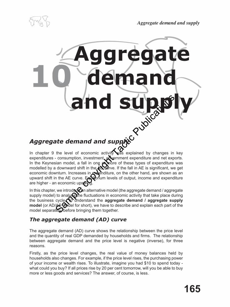
Refer again to figure 10.1. If the price level rose from P3 to P2, households and firms would reduce their aggregate demand for goods and services to a lower level, for the three reasons just described. This is a movement along the AD curve following from a change in the price level.

As we saw in chapter 9, there are a number of factors which could change the willingness of households and firms to spend. Some examples are:• changes in interest rates• changes in taxation levels by government• expectations and confidence levels

If any one of these events happens, assuming there is no change in the price level at the same time, then the whole AD curve would shift, either inwards to the left (bringing about a fall in real output) or outwards to the right (bringing about an increase in real output) Figure 10.2 illustrates some examples of the impact of various events on the AD curve. In the top panels, there is a reduction in aggregate demand as interest rates rise (because the cost of borrowing rises) or because expectations about the future worsen..

A rise in interest rates would .... raise the cost of borrowing for households and firms, so C and I would fall ... hence AD shifts to the left.AD1AD2

Price level

Real output

A fall in business expectations would .... reduce the willingness of businesses to invest ... hence AD shifts to the left.

AD1AD2

Price level

Real output

A depreciation in the exchange rate would .... make exports more competitive and reducethe competitiveness of imports ... hence AD shifts to the right.

AD2AD1

Price level

Real output

The factors identified in figure 9.3 are relevant here as well. Aggregate demand is the total of consumption, investment, government spending and net exports. Aggregate consumption is influenced by disposable income, stock of wealth, interest rates and expectations. Aggregate investment is influenced by levels of retained profit, interest rates, and expectations. Net exports are influenced by domestic and overseas economic activity, tariffs, quotas, exchange rates, terms of trade. The diagrams at left provide three examples of how changes in these factors influence aggregate demand.

Secondly, higher price levels means households and firms need to hold more funds to finance their transactions. They could do this by withdrawing money from banks, borrowing, or selling financial assets such as bonds. The rising demand for money drives interest rates upwards, increasing the cost of borrowing, and acting as a disincentive to spending.

Thirdly, if the domestic price level rises relative to other countries, domestic goods and services become less

competitive in those countries. Other things being equal, this means there will be an increase in imports and a fall in exports.

The three reasons above are often referred to as:• the ‘wealth effect” - the price level affects the real spending power of households

and firms.• the “interest rate effect” - the price level affects interest rates, which impacts

on the cost of borrowing for households and firms.• the “trade effect” or the “international effect” - the price level affects the

competitiveness of domestic goods with their international counterparts.

The AD/price level relationship is illustrated in figure 10.1. Total spending on real output (aggregate demand) is dependent on the price level. The AD/AS model is more powerful than the Keynesian model developed in the last chapter - the AD/AS model brings in changes in the price level (inflation) which the Keynesian model did not include. Note that a change in the price level in the economy will result in a movement along the AD curve. A change in any of the elements of aggregate expenditure (C,I,G,X or M) will bring about a shift of the entire aggregate demand curve .

AE1

AE2

AE 45o

AE3

e1

e2

e3

Real output

e1

e2

e3

AD

P1

P2

P3

Price level

Real output

AE1

AE2

AE3

The aggregate demand curve shows the amount of goods and services that domestic consumers, domestic producers, the government and foreign buyers will collectively want to buy at each price level.

Aggregate purchasing power shifts if the price level changes. An increase in prices would mean that real purchasing power would fall from AE1 to AE2, to AE3. Falling real purchasing power represents reduced demand on the aggregate demand curve in the lower portion of the diagram. Any change in the price level in the economy will result in a movement along the AD curve.

Note that the AD/AS model still labels the x-axis as ‘real output’ - the potential amount of goods and services the economy can produce using available resources. The label on the y-axis is ‘price level’. This could be interpreted as ‘the rate of change in the price level’ - the inflation rate.

Deriving the aggregate demand curve10.1

Shifts in aggregate demand10.2

Sample

copy

right

Tactic

Pub

licati

ons

168 169


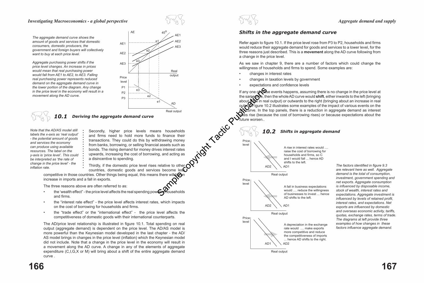
shows the short run relationship between the price level and the quantity of goods and services that firms are willing to offer for sale. In the short run, producers respond to higher demand (and prices) by bringing more inputs into the production process and increasing the utilization of their existing inputs. Aggregate supply responds to changes in price in the short run. In the long run, however, changes in the price level do not affect the level of real GDP. Thus the long run aggregate supply curve (LRAS) shown in panel b of figure 10.4 is vertical.

Shifts in the SRAS curve are caused by unexpected changes in the prices of producer inputs. If real wage levels fell, for example, we would show the whole AS curve shifting to the right. Firms would be willing to produce more output, because their costs have fallen relative to price levels. On the other hand, higher fuel prices, or higher taxation levels, would cause a leftward shift of the whole SRAS curve. Figure 10.4 illustrates some causes of shifts in the aggregate supply curve.

Long run aggregate supply (LRAS) is driven by improvements in productivity and by an expansion of available factor inputs (more firms, a bigger capital stock, an expanding active labour force etc), and the productivity of those inputs. Over time, we would expect an outward shift in the long run supply curve, as the quantity and productivity of productive factors increases.

Explaining equilibrium using the AD/AS modelIn figure 10.5, we bring together the AD, SRAS and LRAS curves. The intersection of the three curves describes long run macroeconomic equilibrium for the economy. Qp indicates the potential output of the economy, given current levels of resources and technology. The price level (Pc) means there is no upward pressure on prices (P constant). At this point, everyone who wants a job can find one, and the economy is operating at normal capacity.

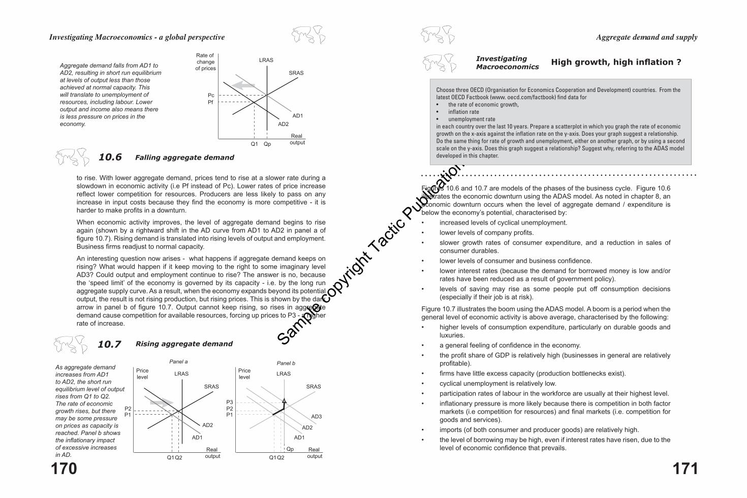
In periods of low economic activity, aggregate demand is less than that which would be required to fully employ resources. This is illustrated in figure 10.6. Aggregate demand falls from AD1 to AD2. Output falls from Qp to Q1. The rate of economic growth is lower than the long run average. Lower output is translated to less demand for the factors of production such as labour and capital equipment, so we would expect levels of investment in new equipment to fall, and we would expect unemployment

Even if everyone who wants a job can find one (i.e. no cyclical unemployment), there would still be frictional (job search) and structural unemployment.

Rate of changeof prices

Real output

SRAS

AD

Pc

Qp

LRAS The intersection of the AD, SRAS and LRAS curves describes long run macroeconomic equilibrium. The level of output (Qp) is at the economy’s potential, given current levels of resources and technology. The price level (Pc) means there is no upward pressure on prices. The model shows an economy operating at its normal capacity.

The aggregate supply curve

The aggregate supply curve shows the level of real domestic output that will be produced at each price level, assuming other influences on production plans remain the same. As illustrated in figure 10.3, the aggregate supply curve is upward sloping because firms are willing to produce more output at higher price levels. Note that the curve in figure 10.3 is the short run aggregate supply curve (SRAS). The SRAS

SRAS and LRAS10.3

A rise in the price of an important input such as oil would .... raise the cost of producing output, so AS shifts to the left.

Price level

Real output

Price level

Real outputPrice level

Real output

An increase in labour productivity would .... reduce the cost of producing output, so AS shifts to the right.

SRAS1SRAS2

A major resource find would .... increase potential output, so AS shifts to the right.

SRAS1SRAS2

SRAS1SRAS2

The short run aggregate supply curve in panel a is upward sloping because firms are willing to employ more resources and produce more output at higher prices. The long run aggregate supply curve in panel b is vertical (not affected by the price level). Over time, we would expect it to shift to the right given more resources (e.g. labour, rising productivity and improved technology).

Price level

Real output

SRAS Price level

Real output

LRAS1 LRAS2

Panel a - short run Panel b - long run

Shifts in short run aggregate supply10.4

Shifts in the SRAS curve are caused by unexpected changes in the prices of producer inputs, and (in common with the LRAS) changes in resource stocks, capital equipment stocks, technology and productivity. If real wage levels fell, for example, we would show the whole AS curve shifting to the right. Firms would be willing to produce more output, because their costs have fallen relative to price levels. On the other hand, higher fuel prices, or higher taxation levels, would cause a leftward shift of the whole SRAS curve.

Macroeconomic equilibrium10.5

Sample

copy

right

Tactic

Pub

licati

ons

170 171


Figures 10.6 and 10.7 are models of the phases of the business cycle. Figure 10.6 illustrates the economic downturn using the ADAS model. As noted in chapter 8, an economic downturn occurs when the level of aggregate demand / expenditure is below the economy’s potential, characterised by:• increased levels of cyclical unemployment.• lower levels of company profits.• slower growth rates of consumer expenditure, and a reduction in sales of

consumer durables. • lower levels of consumer and business confidence. • lower interest rates (because the demand for borrowed money is low and/or

rates have been reduced as a result of government policy).• levels of saving may rise as some people put off consumption decisions

(especially if their job is at risk).

Figure 10.7 illustrates the boom using the ADAS model. A boom is a period when the general level of economic activity is above average, characterised by the following:• higher levels of consumption expenditure, particularly on durable goods and

luxuries.• a general feeling of confidence in the economy.• the profit share of GDP is relatively high (businesses in general are relatively

profitable).• firms have little excess capacity (production bottlenecks exist).• cyclical unemployment is relatively low.• participation rates of labour in the workforce are usually at their highest level.• inflationary pressure is more likely because there is competition in both factor

markets (i.e competition for resources) and final markets (i.e. competition for goods and services).

• imports (of both consumer and producer goods) are relatively high.• the level of borrowing may be high, even if interest rates have risen, due to the

level of economic confidence that prevails.

Choose three OECD (Organisation for Economics Cooperation and Development) countries. From the latest OECD Factbook (www. oecd.com/factbook) find data for • the rate of economic growth,• inflation rate • unemployment rate in each country over the last 10 years. Prepare a scatterplot in which you graph the rate of economic growth on the x-axis against the inflation rate on the y-axis. Does your graph suggest a relationship. Do the same thing for rate of growth and unemployment, either on another graph, or by using a second scale on the y-axis. Does this graph suggest a relationship? Suggest why, referring to the ADAS model developed in this chapter.

High growth, high inflation ?Investigating Macroeconomics

to rise. With lower aggregate demand, prices tend to rise at a slower rate during a slowdown in economic activity (i.e Pf instead of Pc). Lower rates of price increase reflect lower competition for resources. Producers are less likely to pass on any increase in input costs because they find the economy is more competitive - it is harder to make profits in a downturn.

When economic activity improves, the level of aggregate demand begins to rise again (shown by a rightward shift in the AD curve from AD1 to AD2 in panel a of figure 10.7). Rising demand is translated into rising levels of output and employment. Business firms readjust to normal capacity.

An interesting question now arises - what happens if aggregate demand keeps on rising? What would happen if it keep moving to the right to some imaginary level AD3? Could output and employment continue to rise? The answer is no, because the ‘speed limit’ of the economy is governed by its capacity - i.e. by the long run aggregate supply curve. As a result, when the economy expands beyond its potential output, the result is not rising production, but rising prices. This is shown by the dark arrow in panel b of figure 10.7. Output cannot keep rising, so rises in aggregate demand cause competition for available resources, forcing up prices to P3 - a higher rate of increase.


Real output

SRAS

AD1

Pc

Qp

LRAS

Q1

Pf

AD2

Aggregate demand falls from AD1 to AD2, resulting in short run equilibrium at levels of output less than those achieved at normal capacity. This will translate to unemployment of resources, including labour. Lower output and income also means there is less pressure on prices in the economy.

As aggregate demand increases from AD1 to AD2, the short run equilibrium level of output rises from Q1 to Q2. The rate of economic growth rises, but there may be some pressure on prices as capacity is reached. Panel b shows the inflationary impact of excessive increases in AD.

Pricelevel

Real output

SRAS

AD1

P1

Q1

LRAS

Q2

P2

AD2

P3

Qp

AD3

Real output

SRAS

AD1

P1

Q1

LRAS

Q2

P2

AD2

Pricelevel

Panel bPanel a

Rising aggregate demand10.7

Falling aggregate demand10.6

Sample

copy

right

Tactic

Pub

licati

ons

172 173


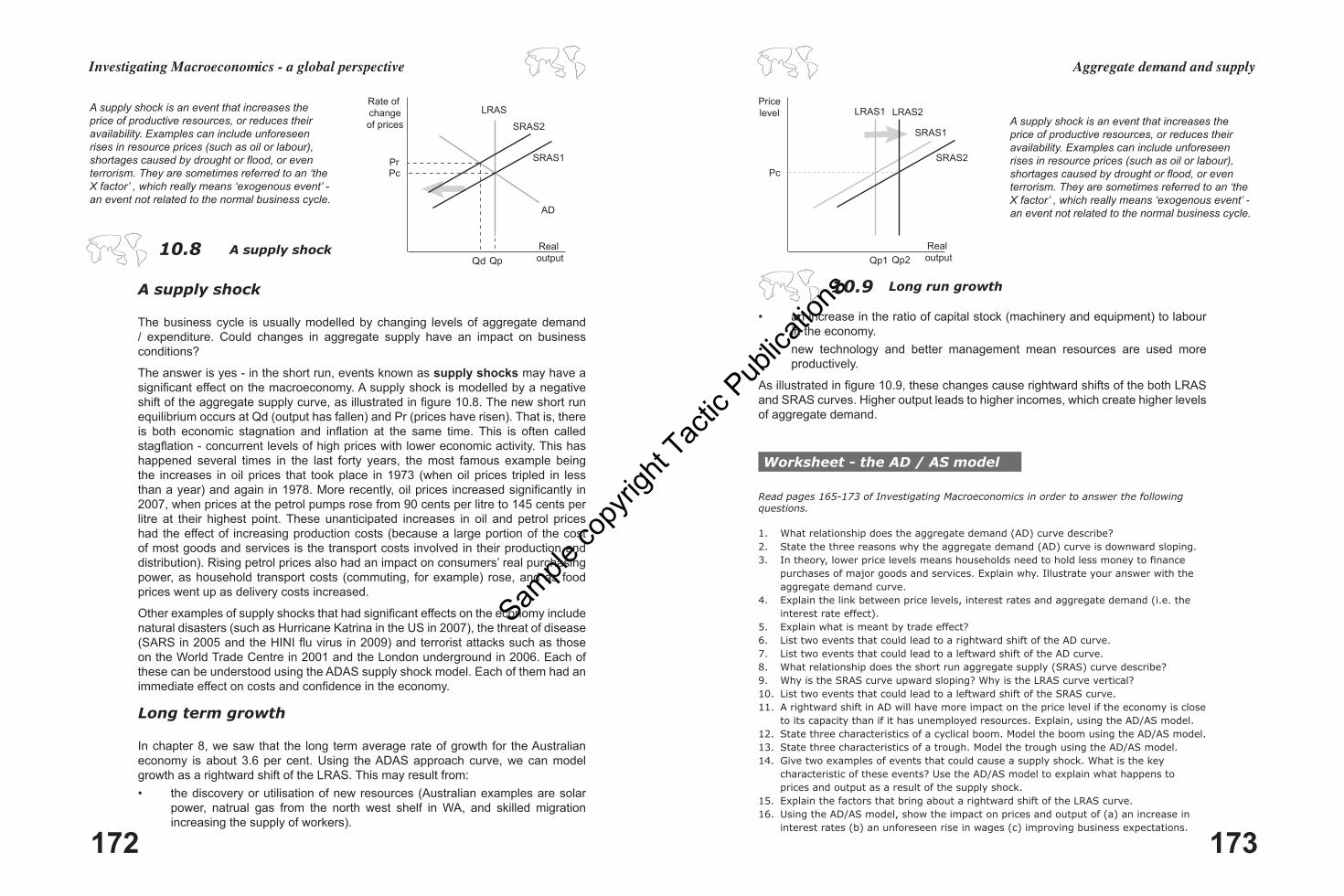
• an increase in the ratio of capital stock (machinery and equipment) to labour in the economy.

• new technology and better management mean resources are used more productively.

As illustrated in figure 10.9, these changes cause rightward shifts of the both LRAS and SRAS curves. Higher output leads to higher incomes, which create higher levels of aggregate demand.

Worksheet - the AD / AS model

Read pages 165-173 of Investigating Macroeconomics in order to answer the following questions.

1. What relationship does the aggregate demand (AD) curve describe?2. State the three reasons why the aggregate demand (AD) curve is downward sloping.3. In theory, lower price levels means households need to hold less money to finance

purchases of major goods and services. Explain why. Illustrate your answer with the aggregate demand curve.

4. Explain the link between price levels, interest rates and aggregate demand (i.e. the interest rate effect).

5. Explain what is meant by trade effect?6. List two events that could lead to a rightward shift of the AD curve. 7. List two events that could lead to a leftward shift of the AD curve. 8. What relationship does the short run aggregate supply (SRAS) curve describe?9. Why is the SRAS curve upward sloping? Why is the LRAS curve vertical?10. List two events that could lead to a leftward shift of the SRAS curve. 11. A rightward shift in AD will have more impact on the price level if the economy is close

to its capacity than if it has unemployed resources. Explain, using the AD/AS model.12. State three characteristics of a cyclical boom. Model the boom using the AD/AS model.13. State three characteristics of a trough. Model the trough using the AD/AS model.14. Give two examples of events that could cause a supply shock. What is the key

characteristic of these events? Use the AD/AS model to explain what happens to prices and output as a result of the supply shock.

15. Explain the factors that bring about a rightward shift of the LRAS curve.16. Using the AD/AS model, show the impact on prices and output of (a) an increase in

interest rates (b) an unforeseen rise in wages (c) improving business expectations.

Pricelevel

Real output

SRAS1

Pc

Qp1

LRAS1

Qp2

LRAS2

SRAS2

A supply shock is an event that increases the price of productive resources, or reduces their availability. Examples can include unforeseen rises in resource prices (such as oil or labour), shortages caused by drought or flood, or even terrorism. They are sometimes referred to an ‘the X factor’ , which really means ‘exogenous event’ - an event not related to the normal business cycle.

A supply shock

The business cycle is usually modelled by changing levels of aggregate demand / expenditure. Could changes in aggregate supply have an impact on business conditions?

The answer is yes - in the short run, events known as supply shocks may have a significant effect on the macroeconomy. A supply shock is modelled by a negative shift of the aggregate supply curve, as illustrated in figure 10.8. The new short run equilibrium occurs at Qd (output has fallen) and Pr (prices have risen). That is, there is both economic stagnation and inflation at the same time. This is often called stagflation - concurrent levels of high prices with lower economic activity. This has happened several times in the last forty years, the most famous example being the increases in oil prices that took place in 1973 (when oil prices tripled in less than a year) and again in 1978. More recently, oil prices increased significantly in 2007, when prices at the petrol pumps rose from 90 cents per litre to 145 cents per litre at their highest point. These unanticipated increases in oil and petrol prices had the effect of increasing production costs (because a large portion of the cost of most goods and services is the transport costs involved in their production and distribution). Rising petrol prices also had an impact on consumers’ real purchasing power, as household transport costs (commuting, for example) rose, and as food prices went up as delivery costs increased.

Other examples of supply shocks that had significant effects on the economy include natural disasters (such as Hurricane Katrina in the US in 2007), the threat of disease (SARS in 2005 and the HINI flu virus in 2009) and terrorist attacks such as those on the World Trade Centre in 2001 and the London underground in 2006. Each of these can be understood using the ADAS supply shock model. Each of them had an immediate effect on costs and confidence in the economy.

Long term growth

In chapter 8, we saw that the long term average rate of growth for the Australian economy is about 3.6 per cent. Using the ADAS approach curve, we can model growth as a rightward shift of the LRAS. This may result from:• the discovery or utilisation of new resources (Australian examples are solar

power, natrual gas from the north west shelf in WA, and skilled migration increasing the supply of workers).


Real output

SRAS1

AD

Pc

Qp

LRAS

SRAS2

Qd

Pr

A supply shock is an event that increases the price of productive resources, or reduces their availability. Examples can include unforeseen rises in resource prices (such as oil or labour), shortages caused by drought or flood, or even terrorism. They are sometimes referred to an ‘the X factor’ , which really means ‘exogenous event’ - an event not related to the normal business cycle.

A supply shock10.8

Long run growth10.9

Sample

copy

right

Tactic

Pub

licati

ons

174 175


3. insurance premiums for operators of passenger aircraft rise.4. retail trade workers win a nine per cent pay rise over three years, subject to

improving their productivity by a similar amount.

Multiple choice questions

Choose the best alternative in the following questions.

1. Which if the following alternatives does NOT explain why the aggregate demand curve is downward sloping?

a. falling price levels reduce real interest rates. b. rising price levels increase real interest rates. c. falling prices increase purchasing power. d. currency depreciation increases overseas purchasing power for Australian goods.

2. Which if the following alternatives does NOT explain why the short run aggregate supply curve (SRAS) is upward sloping?

a. prices rise due to increasing aggregate demand, but the prices of inputs such as wages remain constant.

b. firms being slow to adjust wages. c. prices rise due to increasing aggregate demand, but the prices of inputs such as

wages increase. d. firms may not increase their prices in the short run because the costs of doing so

are high e.g. changing price labels on shelves..

3. A rise in net exports shifts the aggregate a. demand curve to the right. b. demand curve to the left. c. supply curve to the right. d. supply curve to the left.

4. An increase in the value of the Australian dollar relative to the Japanese yen will a. increase aggregate demand in Australia. b. decrease aggregate supply in Australia. c. increase aggregate demand in Japan. d. increase aggregate supply in Japan.

5. A recession overseas would a. increase Australian net exports and increase aggregate supply. b. increase Australian net exports and increase aggregate demand. c. reduce Australian net exports and reduce aggregate demand. d. reduce Australian net exports and increase aggregate demand.

6. Which of the following would NOT cause the AD curve to shift? a. a change in government spending. b. a change in tax rates. c. a change in investment spending. d. a change in the price level.

7. Which of the following would NOT cause an increase (shift to the right) in SRAS? a. an increase in the expected inflation rate. b. a fall in the price of resources, such as wages. c. good weather conditions. d. a reduction in the expected inflation rate.

8. The point where the economy’s LRAS curve, SRAS curve, and AD curves intersect at a single point represents a point where:

a. economic growth is at the long run average level. b. real GDP is equal to its full-employment level. c. the conditions of short-run equilibrium are fulfilled. d. the conditions of long-run equilibrium are fulfilled.

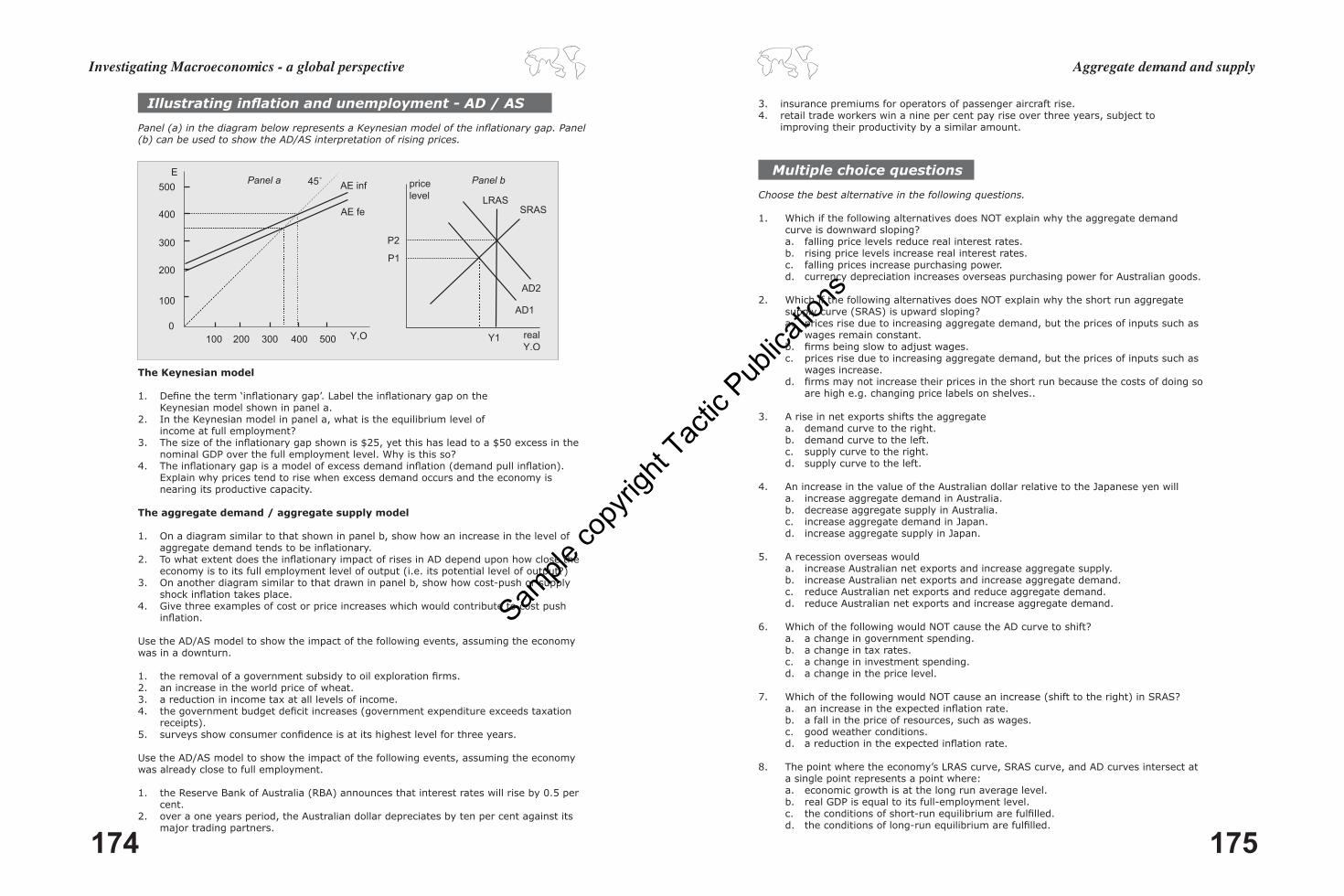
Illustrating inflation and unemployment - AD / AS

Panel (a) in the diagram below represents a Keynesian model of the inflationary gap. Panel (b) can be used to show the AD/AS interpretation of rising prices.

The Keynesian model

1. Define the term ‘inflationary gap’. Label the inflationary gap on the Keynesian model shown in panel a.

2. In the Keynesian model in panel a, what is the equilibrium level of income at full employment?

3. The size of the inflationary gap shown is $25, yet this has lead to a $50 excess in the nominal GDP over the full employment level. Why is this so?

4. The inflationary gap is a model of excess demand inflation (demand pull inflation). Explain why prices tend to rise when excess demand occurs and the economy is nearing its productive capacity.

The aggregate demand / aggregate supply model

1. On a diagram similar to that shown in panel b, show how an increase in the level of aggregate demand tends to be inflationary.

2. To what extent does the inflationary impact of rises in AD depend upon how close the economy is to its full employment level of output (i.e. its potential level of output?)

3. On another diagram similar to that drawn in panel b, show how cost-push or supply shock inflation takes place.

4. Give three examples of cost or price increases which would contribute to cost push inflation.

Use the AD/AS model to show the impact of the following events, assuming the economy was in a downturn.

1. the removal of a government subsidy to oil exploration firms.2. an increase in the world price of wheat.3. a reduction in income tax at all levels of income.4. the government budget deficit increases (government expenditure exceeds taxation

receipts).5. surveys show consumer confidence is at its highest level for three years.

Use the AD/AS model to show the impact of the following events, assuming the economy was already close to full employment.

1. the Reserve Bank of Australia (RBA) announces that interest rates will rise by 0.5 per cent.

2. over a one years period, the Australian dollar depreciates by ten per cent against its major trading partners.

45˚E

Y,O100 200 300 400 500

100

200

300

400

500

0

AE fe

AE inf pricelevel

real Y,O

AD1

SRAS

Y1

P1

Panel a Panel b

P2

AD2

LRAS

Sample

copy

right

Tactic

Pub

licati

ons

176 177


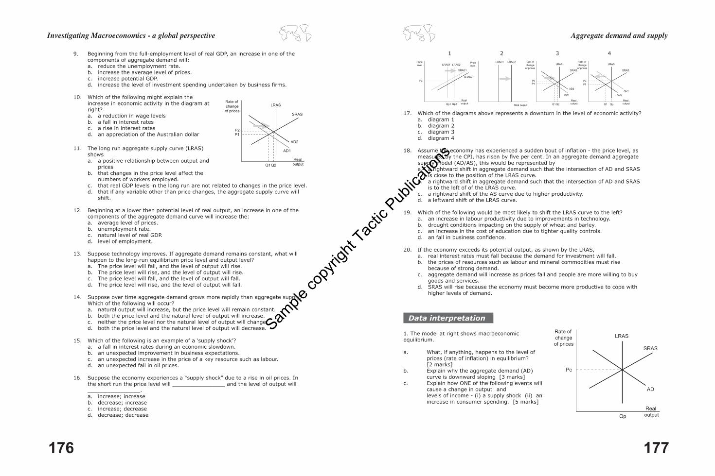
17. Which of the diagrams above represents a downturn in the level of economic activity? a. diagram 1 b. diagram 2 c. diagram 3 d. diagram 4

18. Assume the economy has experienced a sudden bout of inflation - the price level, as measured by the CPI, has risen by five per cent. In an aggregate demand aggregate supply model (AD/AS), this would be represented by

a. a rightward shift in aggregate demand such that the intersection of AD and SRAS is close to the position of the LRAS curve.

b. a rightward shift in aggregate demand such that the intersection of AD and SRAS is to the left of of the LRAS curve.

c. a rightward shift of the AS curve due to higher productivity. d. a leftward shift of the LRAS curve.

19. Which of the following would be most likely to shift the LRAS curve to the left? a. an increase in labour productivity due to improvements in technology. b. drought conditions impacting on the supply of wheat and barley. c. an increase in the cost of education due to tighter quality controls. d. an fall in business confidence.

20. If the economy exceeds its potential output, as shown by the LRAS, a. real interest rates must fall because the demand for investment will fall. b. the prices of resources such as labour and mineral commodities must rise

because of strong demand. c. aggregate demand will increase as prices fall and people are more willing to buy

goods and services. d. SRAS will rise because the economy must become more productive to cope with

higher levels of demand.

Data interpretation

1. The model at right shows macroeconomic equilibrium.

a. What, if anything, happens to the level of prices (rate of inflation) in equilibrium? [2 marks]b. Explain why the aggregate demand (AD) curve is downward sloping [3 marks]c. Explain how ONE of the following events will cause a change in output and levels of income - (i) a supply shock (ii) an increase in consumer spending. [5 marks]

Pricelevel

Real output

SRAS1

Pc

Qp1

LRAS1

Qp2

LRAS2

SRAS2

Price level

Real output

LRAS1 LRAS2 Rate of changeof prices

Real output

SRAS

AD1

Pc

Qp

LRAS

Q1

Pf

AD2


Real output

SRAS

AD1

P1

Q1

LRAS

Q2

P2

AD2

1 2 3 4


Real output

SRAS

AD

Pc

Qp

LRAS

9. Beginning from the full-employment level of real GDP, an increase in one of the components of aggregate demand will:

a. reduce the unemployment rate. b. increase the average level of prices. c. increase potential GDP. d. increase the level of investment spending undertaken by business firms.

10. Which of the following might explain the increase in economic activity in the diagram at right?

a. a reduction in wage levels b. a fall in interest rates c. a rise in interest rates d. an appreciation of the Australian dollar 11. The long run aggregate supply curve (LRAS)

shows a. a positive relationship between output and

prices b. that changes in the price level affect the

numbers of workers employed. c. that real GDP levels in the long run are not related to changes in the price level. d. that if any variable other than price changes, the aggregate supply curve will

shift.

12. Beginning at a lower then potential level of real output, an increase in one of the components of the aggregate demand curve will increase the:

a. average level of prices. b. unemployment rate. c. natural level of real GDP. d. level of employment.

13. Suppose technology improves. If aggregate demand remains constant, what will happen to the long-run equilibrium price level and output level?

a. The price level will fall, and the level of output will rise. b. The price level will rise, and the level of output will rise. c. The price level will fall, and the level of output will fall. d. The price level will rise, and the level of output will fall.

14. Suppose over time aggregate demand grows more rapidly than aggregate supply. Which of the following will occur?

a. natural output will increase, but the price level will remain constant. b. both the price level and the natural level of output will increase. c. neither the price level nor the natural level of output will change. d. both the price level and the natural level of output will decrease.

15. Which of the following is an example of a ‘supply shock’? a. a fall in interest rates during an economic slowdown. b. an unexpected improvement in business expectations. c. an unexpected increase in the price of a key resource such as labour. d. an unexpected fall in oil prices.

16. Suppose the economy experiences a “supply shock” due to a rise in oil prices. In the short run the price level will ________________ and the level of output will ________________.

a. increase; increase b. decrease; increase c. increase; decrease d. decrease; decrease


Real output

SRAS

AD1

P1

Q1

LRAS

Q2

P2

AD2

Sample

copy

right

Tactic

Pub

licati

ons

178

Investigating Macroeconomics - a global perspective

2. This questions refers to the following news extract.

a. Explain what is meant by the term “Australia’s capital stock” [2 marks]b. Explain how the events discussed in the extract would impact of Australia’s long term aggregate supply. [3 marks]c. Explain how the events discussed in the extract would impact on levels of output, income and employment in the Australian economy [5 marks]

Extended writing

Answer each of the following questions in about 2-3 pages of normal writing. Use economic models and examples where appropriate. Pay attention to the specified allocation of marks.

1. (a) Distinguish between the causes of a movement along the aggregate demand curve and a shift of the curve [7 marks]

(b) Explain how an increase in aggregate demand would impact of macroeconomioc equilibrium, assuming the economy was in a trough. [8 marks]

2. (a) Using the aggregate demand/aggregate supply model, explain how changes in injections and leakages impact upon levels of output, income and employment in the economy. [8 marks]

(b) Show how the impact of the following events can be modelled using and aggregate demand aggregate supply framework:

(i) a rise in interest rates.

(ii) a significant unexpected rise in wages.

(iii) a rise in productivity. [12 marks]

3. Using the aggregate demand / aggregate supply (AD/AS) framework, explain how changes in aggregate demand are responsible for (i) rising price levels in an economic upswing and boom and (ii) unemployment of labour in an economic downturn / trough. [20 marks].

4. (a) During 2008 there was a sharp rise in the price of oil and a decrease in house prices in the United States. Using the ADAS model, explain how these events would have influenced the equilibrium level of out in the US economy. [9 marks]

(b) Explain how the large economic stimulus packages used in many parts of the world would impact on levels of spending and output. [6 marks]

5. Explain why the SRAS curve id upward sloping, yet the LRAS curve is vertical. What factors could bring about a rightward shift in either of these curves? [20 marks]

“Huge investment in the resources sector and high migration should allow the Australian economy to grow much faster than its normal trend over the next few years. The reserve Bank of Australia’s quarterly statement on monetary policy says Australia’s capital stock is growing at about 5 per cent a year (faster than its average rate of growth in the 91990’s) and immigration equal to to 2 per cent of population a years is increasing the stock of labour.” (Geoff Winestock, Australian Financial Review, November 7-8, 2009).