Aggregate Demand and Aggregate Supply

Shows the amount of Real GDP that the private, public and foreign sector collectively desire to purchase at each possible price level

The relationship between the price level and the level of Real GDP is inverse See graph

PL

GDPR

AD

Aggregate Demand Curve

Real-Balances Effect When the price-level is high households and

businesses cannot afford to purchase as much output.

When the price-level is low households and businesses can afford to purchase more output.

Interest-Rate Effect A higher price-level increases the interest rate

which tends to discourage investment A lower price-level decreases the interest rate which

tends to encourage investment Foreign Purchases Effect

A higher price-level increases the demand for relatively cheaper imports

A lower price-level increases the foreign demand for relatively cheaper U.S. exports

There are two parts to a shift in AD: A change in C, IG, G and/or XN

A multiplier effect that produces a greater change than the original change in the 4 components

Increases in AD = AD Decreases in AD = AD

PL

GDPR

AD AD1

Increase in Aggregate Demand

PL

GDPR

AD1 AD

Decrease in Aggregate Demand

Consumption (C) Gross Private Investment (IG) Government Spending (G) Net Exports (XN) = Exports - Imports (X – M)

Household spending is affected by: Consumer wealth

More wealth = more spending (AD shifts ) Less wealth = less spending (AD shifts )

Consumer expectations Positive expectations = more spending (AD shifts ) Negative expectations = less spending (AD shifts )

Household indebtedness Less debt = more spending (AD shifts ) More debt = less spending (AD shifts )

Taxes Less taxes = more spending (AD shifts ) More taxes = less spending (AD shifts )

Investment Spending is sensitive to: The Real Interest Rate

Lower Real Interest Rate = More Investment (AD) Higher Real Interest Rate = Less Investment (AD)

Expected Returns Higher Expected Returns = More Investment (AD) Lower Expected Returns = Less Investment (AD) Expected Returns are influenced by

Expectations of future profitability Technology Degree of Excess Capacity (Existing Stock of Capital) Business Taxes

Hyperlink to InvestmentDemand.pps

More Government Spending (AD) Less Government Spending (AD)

Net Exports are sensitive to: Exchange Rates (International value of $)

Strong $ = More Imports and Fewer Exports = (AD ) Weak $ = Fewer Imports and More Exports = (AD )

Relative Income Strong Foreign Economies = More Exports = (AD ) Weak Foreign Economies = Less Exports = (AD )

AD reflects an inverse relationship between PL and GDPR

Δ in PL creates real-balance, interest-rate, and foreign purchase effects that explain AD’s downward slope

Δ in C, IG, G, and/or XN cause Δ in GDPR because they Δ AD.

Increase in AD = AD Decrease in AD = AD

The level of Real GDP (GDPR) that firms will produce at each Price Level (PL)

Long-Run Period of time where

input prices are completely flexible and adjust to changes in the price-level

In the long-run, the level of Real GDP supplied is independent of the price-level

Short-Run Period of time where

input prices are sticky and do not adjust to changes in the price-level

In the short-run, the level of Real GDP supplied is directly related to the price level

The Long-Run Aggregate Supply or LRAS marks the level of full employment in the economy (analogous to PPC)

Because input prices are completely flexible in the long-run, changes in price-level do not change firms’ real profits and therefore do not change firms’ level of output. This means that the LRAS is vertical at the economy’s level of full employment

PL

GDPR

LRAS

Yf

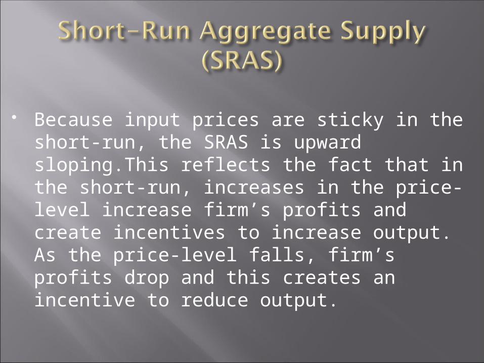
Because input prices are sticky in the short-run, the SRAS is upward sloping.This reflects the fact that in the short-run, increases in the price-level increase firm’s profits and create incentives to increase output. As the price-level falls, firm’s profits drop and this creates an incentive to reduce output.

PL

GDPR

SRAS

An increase in SRAS is seen as a shift to the right. SRAS

A decrease in SRAS is seen as a shift to the left. SRAS

The key to understanding shifts in SRAS is per unit cost of production

Per-unit production cost = total input cost/total output

PL

GDPR

SRAS SRAS1

PL

GDPR

SRASSRAS1

Input Prices

Productivity

Legal-Institutional Environment

Domestic Resource Prices Wages (75% of all business costs) Cost of capital Raw Materials (commodity prices)

Foreign Resource Prices Strong $ = lower foreign resource prices Weak $ = higher foreign resource prices

Market Power Monopolies and cartels that control resources

control the price of those resources Increases in Resource Prices = SRAS Decreases in Resource Prices = SRAS

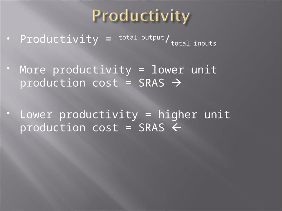
Productivity = total output/total inputs

More productivity = lower unit production cost = SRAS

Lower productivity = higher unit production cost = SRAS

Taxes and Subsidies Taxes ($ to gov’t) on business increase per unit

production cost = SRAS Subsidies ($ from gov’t) to business reduce per unit

production cost = SRAS Government Regulation

Government regulation creates a cost of compliance = SRAS

Deregulation reduces compliance costs = SRAS

The equilibrium of AS & AD determines current output (GDPR) and the price level (PL)

GDPR

PL

AD

SRASLRAS

YF

P

Full Employment equilibrium exists where AD intersects SRAS & LRAS at the same point.

GDPR

PL

AD

SRASLRAS

YF

P

A recessionary gap exists when equilibrium occurs below full employment output.

GDPR

PL

AD

SRASLRAS

YF

P

Y

An inflationary gap exists when equilibrium occurs beyond full employment output.

GDPR

PL

AD

SRASLRAS

YF

P

Y

Δ Consumption (C) C↑ .: AD .: GDPR↑ & PL↑ .: u%↓ & π%↑ C↓ .: AD .: GDPR↓ & PL↓ .: u%↑ & π%↓

Δ Gross Private Investment (IG) IG↑ .: AD .: GDPR↑ & PL↑ .: u%↓ & π%↑ IG↓ .: AD .: GDPR↓ & PL↓ .: u%↑ & π%↓

Δ Government Spending (G) G↑ .: AD .: GDPR↑ & PL↑ .: u%↓ & π%↑ G↓ .: AD .: GDPR↓ & PL↓ .: u%↑ & π%↓

Δ Net Exports (XN) XN↑ .: AD .: GDPR↑ & PL↑ .: u%↓ & π%↑ XN↓ .: AD .: GDPR↓ & PL↓ .: u%↑ & π%↓

C↑, IG↑, G↑ and/or XN↑ .: AD .: GDPR↑ & PL↑ .: u%↓ & π%↑

GDPR

PL

AD

SRASLRAS

YF

P

Y

AD1

P1

C↓, IG↓, G↓ and/or XN↓ .: AD .: GDPR↓ & PL↓ .: u%↑ & π%↓

GDPR

PL

AD

SRAS

LRAS

YF

P

Y

AD1

P1

Δ Input Prices Input Prices↓ .: SRAS .: GDPR↑ & PL↓ .: u%↓ & π%↓

Input Prices↑ .: SRAS .: GDPR↓ & PL ↑ .: u%↑ & π%↑

Δ Productivity Productivity↑ .: SRAS .: GDPR↑ & PL↓ .: u%↓ & π%↓

Productivity↓ .: SRAS .: GDPR↓ & PL ↑ .: u%↑ & π%↑

Δ Legal-Institutional Environment Deregulation .: SRAS .: GDPR↑ & PL↓ .: u%↓ & π%↓

Regulation .: SRAS .: GDPR↓ & PL ↑ .: u%↑ & π%↑

Input Prices↓, Productivity↑, and/or Deregulation .: SRAS .: GDPR↑ & PL↓ .: u%↓ & π%↓

GDPR

PL

AD

SRASLRAS

YF

P

Y

SRAS1

P1

Input Prices↑, Productivity↓, and/or Regulation .: SRAS .: GDPR↓ & PL↑ .: u%↑ & π%↑

GDPR

PL

AD

SRAS

LRAS

YF

P

Y1

SRAS1

P1

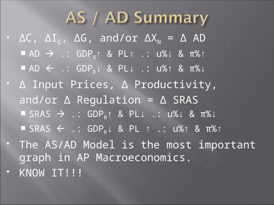
ΔC, ΔIG, ΔG, and/or ΔXN = Δ AD AD .: GDPR↑ & PL↑ .: u%↓ & π%↑

AD .: GDPR↓ & PL↓ .: u%↑ & π%↓

Δ Input Prices, Δ Productivity, and/or Δ Regulation = Δ SRAS SRAS .: GDPR↑ & PL↓ .: u%↓ & π%↓

SRAS .: GDPR↓ & PL ↑ .: u%↑ & π%↑

The AS/AD Model is the most important graph in AP Macroeconomics.

KNOW IT!!!