AFRL-RX-TY-TR-2013-0005
ADVANCED COMPUTATION DYNAMICS SIMULATION OF PROTECTIVE STRUCTURES RESEARCH
Daniel G. Brannon and James S. Davidson Department of Civil Engineering Auburn University 238 Harbert Engineering Center Auburn, AL 36849
For Universal Technology Corporation 1270 North Fairfield Road Dayton, OH 45432-2600
Contract No. FA8650-07-D-5800-0044 February 2013
DISTRIBUTION A. Approved for public release; distribution unlimited. 88ABW-2013-2703, 6 June 2013.
AIR FORCE RESEARCH LABORATORY MATERIALS AND MANUFACTURING DIRECTORATE
Air Force Materiel Command United States Air Force Tyndall Air Force Base, FL 32403-5323
DISCLAIMER
Reference herein to any specific commercial product, process, or service by trade name,
trademark, manufacturer, or otherwise does not constitute or imply its endorsement,
recommendation, or approval by the United States Air Force. The views and opinions of
authors expressed herein do not necessarily state or reflect those of the United States Air
Force.
This report was prepared as an account of work sponsored by the United States Air Force.
Neither the United States Air Force, nor any of its employees, makes any warranty,
expressed or implied, or assumes any legal liability or responsibility for the accuracy,
completeness, or usefulness of any information, apparatus, product, or process disclosed, or
represents that its use would not infringe privately owned rights.

NOTICE AND SIGNATURE PAGE Using Government drawings, specifications, or other data included in this document for any purpose other than Government procurement does not in any way obligate the U.S. Government. The fact that the Government formulated or supplied the drawings, specifications, or other data does not license the holder or any other person or corporation; or convey any rights or permission to manufacture, use, or sell any patented invention that may relate to them. This report was cleared for public release by the and is aa and is nationals. Copies may be obtained from the Defense Technical Information Center (DTIC) (http://www.dtic.mil). HAS BEEN REVIEWED AND IS APPROVED FOR PUBLICATION IN ACCORDANCE WITH ASSIGNED DISTRIBUTION STATEMENT. ______________________________________ ______________________________________ This report is published in the interest of scientific and technical information exchange, and its publication does not constitute the Government’s approval or disapproval of its ideas or findings.
88th Air Base Wing Public Affairs Office atWright Patterson Air Force Base, Ohio available to the general public, including foreign
AFRL-RX-TY-TR-2013-0005
Chief, Airbase Technologies Division
ALBERT N. RHODES, PhD
Work Unit Manager
DEBRA L. RICHLIN, DR-III
///SIGNED///
///SIGNED///
Standard Form 298 (Rev. 8/98)
REPORT DOCUMENTATION PAGE
Prescribed by ANSI Std. Z39.18
Form Approved OMB No. 0704-0188
The public reporting burden for this collection of information is estimated to average 1 hour per response, including the time for reviewing instructions, searching existing data sources, gathering and maintaining the data needed, and completing and reviewing the collection of information. Send comments regarding this burden estimate or any other aspect of this collection of information, including suggestions for reducing the burden, to Department of Defense, Washington Headquarters Services, Directorate for Information Operations and Reports (0704-0188), 1215 Jefferson Davis Highway, Suite 1204, Arlington, VA 22202-4302. Respondents should be aware that notwithstanding any other provision of law, no person shall be subject to any penalty for failing to comply with a collection of information if it does not display a currently valid OMB control number. PLEASE DO NOT RETURN YOUR FORM TO THE ABOVE ADDRESS. 1. REPORT DATE (DD-MM-YYYY) 2. REPORT TYPE 3. DATES COVERED (From - To)
4. TITLE AND SUBTITLE 5a. CONTRACT NUMBER
5b. GRANT NUMBER
5c. PROGRAM ELEMENT NUMBER
5d. PROJECT NUMBER
5e. TASK NUMBER
5f. WORK UNIT NUMBER
6. AUTHOR(S)
7. PERFORMING ORGANIZATION NAME(S) AND ADDRESS(ES) 8. PERFORMING ORGANIZATION REPORT NUMBER
9. SPONSORING/MONITORING AGENCY NAME(S) AND ADDRESS(ES) 10. SPONSOR/MONITOR'S ACRONYM(S)
11. SPONSOR/MONITOR'S REPORT NUMBER(S)
12. DISTRIBUTION/AVAILABILITY STATEMENT
13. SUPPLEMENTARY NOTES
14. ABSTRACT
15. SUBJECT TERMS
16. SECURITY CLASSIFICATION OF: a. REPORT b. ABSTRACT c. THIS PAGE
17. LIMITATION OF ABSTRACT
18. NUMBER OF PAGES
19a. NAME OF RESPONSIBLE PERSON
19b. TELEPHONE NUMBER (Include area code)
01-FEB-2013 Final Technical Report 08-JAN-2009 -- 31-JAN-2013
Advanced Computation Dynamics Simulation of Protective Structures Research
FA8650-07-D-5800-0044
0909999F
GOVT
F0
X00H (QF101007)
Brannon, Daniel G.; Davidson, James S.
Conducted by: Auburn University, Department of Civil Engineering, 238 Harbert Engineering Center, Auburn, AL 36849 Conducted for: Universal Technology Corporation, 1270 North Fairfield Road. Dayton, OH 45432-2600
Air Force Research Laboratory Materials and Manufacturing Directorate Airbase Technologies Division 139 Barnes Drive, Suite 2 Tyndall Air Force Base, FL 32403-5323
AFRL/RXQ
AFRL-RX-TY-TR-2013-0005
DISTTRIBUTION A: Approved for public release; distribution unlimited.
Ref Public Affairs Case # 88ABW-2013-2703, 6 June 2013. Document contains color images.
This report presents the results of an investigation involving finite element simulation of partially grouted concrete masonry walls subjected to blast loading and the development of an engineering design equation to address the potential for breaching between grouted cells. Tests performed by the Air Force Research Laboratory were used to verify finite element modeling approach. Input parameter studies were carried out to understand the mechanisms and causes of the breaching shear in concrete masonry walls. Based upon the mechanism findings, a design shear equation was formulated, and a maximum pressure for partially grouted construction was defined.
concrete masonry units, masonry construction, direct shear, partially grouted, finite element modeling, breaching, quasi-static
U U U UU 95
Jason P. Lowery
Reset
i DISTRIBUTION STATEMENT A. Approved for public release; distribution unlimited.
88ABW-2013-2703 6 Jun 2013.
TABLE OF CONTENTS
LIST OF FIGURES ....................................................................................................................... iii LIST OF TABLES ...........................................................................................................................v 1. SUMMARY .........................................................................................................................1 2. INTRODUCTION ...............................................................................................................2 2.1. Overview ..............................................................................................................................2 2.2. Objective ..............................................................................................................................2 2.3. Scope and Methodology ......................................................................................................3 2.4. Report Organization .............................................................................................................3 2.5. Literature Overview .............................................................................................................3 2.6. Concrete Masonry Units ......................................................................................................4 2.6.1. Flexural Behavior.................................................................................................................4 2.6.2. Shear Behavior .....................................................................................................................5 2.7. Mortar Properties .................................................................................................................6 2.8. Blast Loading .......................................................................................................................7 2.9. Finite Element Modeling .....................................................................................................8 2.9.1. Constitutive Models for CMU .............................................................................................8 2.9.2. CMU Models .......................................................................................................................9 3. METHODS, ASSUMPTIONS, AND PROCEDURES .....................................................11 3.1. Overview ............................................................................................................................11 3.2. Dynamic Testing Overview ...............................................................................................11 3.2.1. Test Set-up .........................................................................................................................11 3.2.2. Test Results ........................................................................................................................15 3.3. Unit System ........................................................................................................................17 3.4. Geometry and Meshing ......................................................................................................18 3.4.1. Concrete Masonry Units ....................................................................................................18 3.4.2. Mortar and Grout ...............................................................................................................20 3.4.3. Steel Reinforcing ...............................................................................................................22 3.5. Material Modeling .............................................................................................................23 3.5.1. Cementitious Material Model ............................................................................................23 3.5.2. Reinforcement Material Model ..........................................................................................25 3.5.3. Boundary Material Model ..................................................................................................26 3.6. Element Modeling ..............................................................................................................26 3.7. Load Modeling ...................................................................................................................27 3.7.1. Gravity Preloading .............................................................................................................27 3.7.2. Blast Loading .....................................................................................................................28 3.8. Boundary Modeling ...........................................................................................................28 3.9. Contact Modeling...............................................................................................................29 3.9.1. Mortar-Block Interface ......................................................................................................29 3.9.2. Block-Boundary Interface ..................................................................................................31 3.10. FEM Validation .................................................................................................................32 3.11. FEM Results and Parametric Study of Breaching .............................................................42 4. RESULTS AND DISCUSSIONS ......................................................................................66 4.1. Introduction ........................................................................................................................66 4.2. Structural Dynamics...........................................................................................................66 4.2.1. SDOF Model ......................................................................................................................66
ii DISTRIBUTION STATEMENT A. Approved for public release; distribution unlimited.
88ABW-2013-2703 6 Jun 2013.
4.2.2. Pressure-Impulse Simplifications ......................................................................................69 4.3. Modeling of Breaching Response ......................................................................................72 4.3.1. Dynamics of the Face Shell Beam Model ..........................................................................72 4.3.2. Dynamics of Between Grout Cells Beam ..........................................................................75 4.3.3. Direct Shear Modeling .......................................................................................................79 4.4. Resistance Equation Derivation .........................................................................................80 4.4.1. Development of Resistance Equation ................................................................................80 4.5. Comparison between FEM Stress and Analytical Stress ...................................................81 4.5.1. Face Shell Beam Comparison ............................................................................................81 4.5.2. Between Grout Cells Beam Comparison ...........................................................................82 4.5.3. Differences between FEM and Analytical Shear Stress ....................................................84 4.6. Breaching Shear Design Equation .....................................................................................85 5. CONCLUSIONS AND RECOMMENDATIONS ............................................................87 5.1. Conclusions ........................................................................................................................87 5.2. Recommendations ..............................................................................................................87 6. REFERENCES ..................................................................................................................88 LIST OF SYMBOLS, ABBREVIATIONS, AND ACRONYMS ................................................90
iii DISTRIBUTION STATEMENT A. Approved for public release; distribution unlimited.
88ABW-2013-2703 6 Jun 2013.
LIST OF FIGURES
Page Figure 1. Pressure Loading Profile ................................................................................................. 8 Figure 2. Front View of 8-in CMU Panel ..................................................................................... 12 Figure 3. Design Details of the 8-in CMU Panel .......................................................................... 13 Figure 4. Panels in Reaction Structure Prior to Testing ............................................................... 14 Figure 5. Video Captures of Breaching of 8-in CMU Wall During Test 2 .................................. 16 Figure 6. Breached 8-in CMU Wall after Test 2 .......................................................................... 17 Figure 7. FEM CMU Mesh and Dimensions ................................................................................ 19 Figure 8. 3-D View of CMU Mesh ............................................................................................... 19 Figure 10. Half-High Block Mesh ................................................................................................ 20 Figure 12. Grout Columns ............................................................................................................ 22 Figure 13. Bond Beam and Blocks ............................................................................................... 22 Figure 15. Qualitative Base Reaction Forces under Gravity Loading .......................................... 28 Figure 16. Boundary Set-Up ......................................................................................................... 29 Figure 17. Mortar-Black Interface ................................................................................................ 31 Figure 18. Boundary-Block Interface ........................................................................................... 32 Figure 19. Test Set-Up and Instrumentation Position ................................................................... 32 Figure 20. Normalized Reflected Pressure from Dynamic Testing .............................................. 33 Figure 21. Normalized Impulse from Dynamic Testing ............................................................... 33 Figure 22. Video Captures of Panel 2 During Test 1 at a) 10 ms, b) 21 ms, c) 41 ms, and d) 84 ms after Loading Starts ................................................................................................................. 34 Figure 23. Deformation of Panel 2 Test 1 at a) 10 ms, b) 21 ms, c) 41 ms, and d) 84 ms after Loading Starts ............................................................................................................................... 35 Figure 24. Deflection Comparison of Panel 2 and FEM from Test 1 ........................................... 36 Figure 25. Video Captures of Panel 2 During Test 2 at a) 10 ms, b) 19 ms, c) 43 ms, and d) 76 ms after Loading Starts ................................................................................................................. 37 Figure 26. Deformation of Panel 2 Test 2 at a) 10 ms, b) 19 ms, c) 43 ms, and d) 76 ms after Loading Starts ............................................................................................................................... 38 Figure 27. Cross-Section Deformation from FEM Results .......................................................... 39 Figure 28. Stress Contours 1 ms after Loading: a) Effective Stress, b) XY-Shear Stress, c) XZ-Shear Stress, and d) Plastic Strain................................................................................................. 40 Figure 29. Deflection Comparison of Panel 2 and FEM from Test 2 ........................................... 41 Figure 30. Deflection Comparison of Panel 2 and FEM from Test 3 ........................................... 41 Figure 31. Contour Plots of Out-of-Plane Shear Stress ................................................................ 43 Figure 35. Contour Plots of Out-of-Plane Shear Stress ................................................................ 47 Figure 36. Contour Plots of Out-of-Plane Shear Stress ................................................................ 48 Figure 37. Contour Plots of Effective Stress at Various Times to 2 ms ....................................... 49 Figure 38. Contour Plots of Effective Stress at Various Times to 5 ms ....................................... 50 Figure 39. Contour Plots of Effective Stress at Various Times to 20 ms ..................................... 51 Figure 40. Out-of-Plane Shear Stress vs. Time............................................................................. 52 Figure 41. Effective Stress vs. Time ............................................................................................. 52 Figure 42. Geometry vs. Shear Stress ........................................................................................... 54 Figure 43. Geometry vs. Effective Stress ..................................................................................... 55 Figure 44. Out-of-Plane Shear Stress vs. Compressive Strength.................................................. 56 Figure 45. Effective Stress vs. Compressive Strength .................................................................. 57
iv DISTRIBUTION STATEMENT A. Approved for public release; distribution unlimited.
88ABW-2013-2703 6 Jun 2013.
Figure 46. Out-of-Plane Shear Stress vs. Unit Weight ................................................................. 58 Figure 47. Effective Stress vs. Unit Weight ................................................................................. 59 Figure 48. Normalized Loading Distribution................................................................................ 60 Figure 50. Effective Stress vs. Peak Pressure ............................................................................... 63 Figure 51. Out-of-Plane Shear Stresses for Grouted and Non-Grouted Walls ............................. 65 Figure 52. Effective Stresses for Grouted and Non-Grouted Walls ............................................. 65 Figure 53. SDOF Idealization ....................................................................................................... 66 Figure 56. Face Shell Beam and Cross Section ............................................................................ 72 Figure 58. BGC Beam and Cross Section A-A............................................................................. 75 Figure 59. Qualitative Effects: Minimum Load Duration vs. Modulus of Elasticity ................... 77 Figure 60. Qualitative Effects: Minimum Load Duration vs. Thickness of Face Shell................ 77 Figure 61. Qualitative Effects: Minimum Load Duration vs. Width of Block ............................. 78 Figure 62. Qualitative Effects: Minimum Load Duration vs. Unit Weight .................................. 78 Figure 63. Minimum Load Duration vs. Length between Grout Cells ......................................... 79 Figure 64. Comparison between FEM and Calculated Shear Stress for Face Shell Beam ........... 82 Figure 65. FEM vs. Calculated Shear Stress for BGC Beam ....................................................... 84 Figure 66. Ratio of FEM to Calculated Shear Stress vs. Length .................................................. 84
v DISTRIBUTION STATEMENT A. Approved for public release; distribution unlimited.
88ABW-2013-2703 6 Jun 2013.
LIST OF TABLES
Page Table 1. Modulus of Rupture Values from ACI 530-11 ................................................................. 7 Table 2. Scaled Standoff ............................................................................................................... 11 Table 3. Test Wall Construction ................................................................................................... 12 Table 4. Materials Properties ........................................................................................................ 15 Table 5. Unit System..................................................................................................................... 17 Table 6. CMU Material Model Selection ..................................................................................... 24 Table 8. Maximum Out-of-Plane Shear Stresses of Various Wall Geometries ............................ 53 Table 9. Maximum Effective Stresses of Various Wall Geometries ............................................ 54 Table 10. Stresses for Compressive Strength Parametric Study ................................................... 55 Table 11. Stresses for Compressive Strength Parametric Study ................................................... 58 Table 12. Stresses from Loading Shape Parametric Study ........................................................... 60 Table 13. Statistical Data from the Loading Shape Parametric Study .......................................... 61 Table 14. Stresses from the 5 × 5 Wall from the Peak Pressure Parametric Study ...................... 61 Table 15. Stresses from the 10 × 3 Wall from the Peak Pressure Parametric Study .................... 62 Table 16. Stresses from the 3 × 10 Wall of the Peak Pressure Parametric Study ......................... 62 Table 17. Grouted vs. Non-Grouted Maximum Stresses .............................................................. 64 Table 18. Representative Numbers for 8-in CMU ........................................................................ 74 Table 19. Loading Regime Ranges ............................................................................................... 74 Table 21. Shear Stress Comparison for Face Shell Beam ............................................................ 82 Table 22. Shear Stress Comparison for BGC Beam ..................................................................... 83 Table 23. Maximum Pressure for Single Block Beam ................................................................. 86 Table 24. Maximum Pressure for BGC Beams ............................................................................ 86
1 DISTRIBUTION STATEMENT A. Approved for public release; distribution unlimited.
88ABW-2013-2703 6 Jun 2013.
1. SUMMARY
This report presents the results of an investigation involving finite element simulation of partially grouted concrete masonry walls subjected to blast loading and the development of an engineering design equation to address the potential for breaching between grouted cells. Tests performed by the Air Force Research Laboratory (AFRL) were used to verify a finite element modeling approach. Input parameter studies were carried out to understand the mechanisms and causes of the breaching shear in concrete masonry walls. Based upon the mechanism findings, a design shear equation was formulated, and a maximum pressure for partially grouted construction was defined.
2 DISTRIBUTION STATEMENT A. Approved for public release; distribution unlimited.
88ABW-2013-2703 6 Jun 2013.
2. INTRODUCTION
2.1. Overview
Starting in World War II, researchers began to look into ways to mitigate the forces caused by blast. During the Cold War, the threat of large scale nuclear threats lead to research in whole system structural response to blasts. However, the Oklahoma City Bombing and World Trade Center Bombing in the 1990s demonstrated the damaging effects of more localized blasts. The use of improvised explosive devices following “9/11” gave greater importance to research on localized response and local phenomenon. High order explosions cause a time-varying load that can result in extreme deflections and high accelerations. However, unlike forces resulting from typical design loads such as wind and earthquakes, blast loading cannot be readily transformed into equivalent static forces. Blast analysis requires that the structure be analyzed as a dynamic system. Blast loading, like earthquake response, is not typically expected to be endured without damage. Also, although potentially catastrophic, an explosion load event is considered to be rare and random. Therefore, the primary objective of blast design criteria focuses on the preservation of life, rather than the prevention of damage. One of the primary concerns is that the loading can produce breaching of the cladding leading to high velocity fragmentation or allowing the blast wave to enter into the structure. Both can cause injuries and loss of life. Masonry is one of the most common types of building material, and has been used for millennia. The first buildings were crude stacks of natural stone; this eventually transitioned into manufactured stone with mortar and into brick and mortar. Starting in the 1800s, concrete masonry units (CMU) began to be used for a wide range of building applications. In modern society, CMU is commonly used as shear walls to resist lateral loads and as cladding on the exterior of structures. This is because masonry is relatively inexpensive, is easily and quickly constructed, and provides insulation for the structure. However, unreinforced CMU walls are weak in flexure and must be grouted and reinforced to handle significant transverse loading. Since grouting every cell of the CMU can be costly, owners and contractors often only grout reinforced cells (partially grouted). Due to the brittleness of unreinforced masonry, the DoD Antiterrorism/Force Protection Construction Standards (DoD 2007) prohibits the use of unreinforced CMU exterior walls for new military construction. However, partially grouted CMU walls are allowed as long as the system is designed to meet the flexural demand (UFC, 2008). A recent experimental study (Davidson et al., 2011) on partially grouted walls has shown that blast loading can cause localized fracturing at relatively low impulse loads. Therefore, partially grouted walls can fragment in dangerous brittle modes under blast impulse loading similar to unreinforced masonry walls. 2.2. Objective
The overall objectives of the research represented by this report were (1) to develop an understanding of the causes of breaching of partially grouted CMU walls subjected to blast loading by using advanced finite element modeling and (2) to develop an engineering-level
3 DISTRIBUTION STATEMENT A. Approved for public release; distribution unlimited.
88ABW-2013-2703 6 Jun 2013.
analytical methodology that can be used to predict direct shear and breaching in partially grouted CMU walls. 2.3. Scope and Methodology
In order to achieve the objectives, tasks included a literature review, development of finite element models, a parametric study, and development of an engineering resistance definition. The finite element models were created and visualized in LS-PrePost and analyzed using the LS-DYNA finite element solver. Full-scale static and dynamic testing results were used to verify the modeling approach. The testing data used for validation was from a prior study by the AFRL (Davidson et al., 2011) whose objectives were to evaluate the behavior of minimally reinforced partially grouted walls subjected to blast loading. The engineering resistance methodology was derived by examining the behavior of the finite element models, and structural dynamic and quasi-static models of CMU were created to approximate the breaching behavior. 2.4. Report Organization
This report is divided into five sections in addition to the summary. Section 2 consists of an introduction, objectives, scope and methodology, and organization of the report. Section 2 also provides a literature review including a brief look at the literature on blast loading, concrete masonry units, mortar, and finite element modeling. Section 3 provides a summary of the finite element methodology, a verification of the finite element modeling, and a parametric study of the breaching phenomenon. Section 4 discusses the breaching and shearing behavior of CMU due to blast loading and presents the development of the design methodology. Section 5 summarizes the results and provides recommendations for designers and researchers. 2.5. Literature Overview
With the increase in terrorist activity across the world, there has arisen a focus on designing and constructing structures to be more resistant to blast loading. Many researchers have investigated the blast resistance of a vast array of construction materials including steel, reinforced concrete, and masonry. Since concrete masonry is a very common type of building material used for exteriors walls, many researchers have looked into improving the performance of masonry subjected to blast loading. Since masonry has very low tensile strength, the wall performs poorly in flexure unless a ductile reinforcement is added into the system. In order to do this, reinforcing steel is added into the hollow cells of the CMU. To provide composite action between the steel and CMU, grout, a flowable concrete mixture, is placed into the reinforced cells. If grout is placed into every cell (including cells without reinforcing steel), the wall is said to be fully grouted. To minimize costs, it is common to add grout only to cells that are reinforced with steel. If this is done, the wall is said to be partially grouted. Over the years, a great deal of work has gone into modeling masonry walls that are unreinforced, reinforced, or fully grouted; several researches have also looked at catcher systems and energy absorption systems. However, there is a general lack of research into partially grouted reinforced masonry wall systems and the difference in their failure mechanics. This report focuses on the
4 DISTRIBUTION STATEMENT A. Approved for public release; distribution unlimited.
88ABW-2013-2703 6 Jun 2013.
phenomenon where there is a direct shear breaching that occurs between the grout columns. The direct shear or breaching shear causes shear cracks to form in the block. 2.6. Concrete Masonry Units
2.6.1. Flexural Behavior The static flexural behavior of CMU has been researched thoroughly. The masonry section of Unified Facilities Criteria (UFC) 3-340-02 (UFC, 2008) states that the method of calculating ultimate moment of combined joint and cell reinforced masonry is the same as that presented in the chapter on concrete. UFC 3-340-02 gives the ultimate moment capacity, Mn, for a concrete beam or non-load bearing wall as
( - )n s dsM A f d a/2= (1) where As = area of the reinforcement, fds = dynamic yield strength of the steel reinforcement, d = distance between the centroid of the tension reinforcement and extreme compression fiber, and a = the depth of the equivalent rectangular compressive block. UFC 3-340-02 makes no distinction between fully grouted and partially grouted walls. This is because research has shown that both types of grouting perform as reinforced concrete if the wall is designed properly. UFC 3-340-02 also establishes rules and guidelines for damage levels from “lightly damaged” to “collapse” and presents design methodology for one-way and two-way action slabs. Davidson et al. (2011) tested several partially grouted CMU walls under uniform static pressure in vacuum chambers. These walls were made of 8-in and 6-in CMU with minimum reinforcing and only the reinforced cells grouted. The walls were loaded by pressure and self-weight; the pressure was uniform over the entire wall surface and increased until the wall collapsed. The walls first cracked along the bed joint at the course nearest to mid-height of the wall, and were able to carry additional load with increased cracking and deflection. Eventually, the walls failed in flexure due to self-weight and did not indicate any signs of shear failure. Plots of midheight deflection versus applied pressure were created, which showed that the resistance of the wall can be described by three behavioral regions. The first is linear-elastic resistance until cracking, followed by a nonlinear resistance caused by changing progression of cracking and straining of steel, and finally ductile displacement under a constant load until collapse. In a related study, Davidson et al. (2011) tested three identically constructed panels under blast loading. In several of the walls, the failure mechanism changed from a ductile failure in flexure to a brittle failure in breaching. The breaching occurred between the grouted cells, typically occurring at the interface between grouted and ungrouted blocks. Davidson et al. (2011) was used as the primary driver for the present work and data from the report was used to validate models used herein. Burrett et al. (2007) tested many full scale CMU walls under impact loading. In their research, they developed finite element models to simulate the impact and resulting damage and derived analytical resistance models of unreinforced, ungrouted walls. In their analytical modeling, they performed a parametric study to define the key components of the resistance functions.
5 DISTRIBUTION STATEMENT A. Approved for public release; distribution unlimited.
88ABW-2013-2703 6 Jun 2013.
Gilbert et al. (2002) developed a rigid-body mechanism analysis of unreinforced masonry walls. In this analysis, rocking, sliding, and a combination of rocking and sliding were analyzed for impact. Five wall-failure mechanisms were found as analysis tools for the prediction of failure and displacement. The analysis allows for the prediction of the peak displacement within a ten percent upper and lower bound. Analyses correlated well with the displacement for all failure modes except one. Sudame (2004) developed a finite element modeling approach that predicts the overall resistance of ungrouted walls subjected to blast loading. Moradi (2008) expanded upon Sudame’s work by modeling of retrofit unreinforced masonry wall systems. Resistance functions were developed for three different retrofits, which were compared to data of walls subjected to blast load testing. 2.6.2. Shear Behavior In Masonry Structures Behavior and Design (Drysdale and Hamid, 2008), the nominal shear strength, Vn, is generalized by
n m sV V V= + (2) where Vm = strength provided by the masonry, and Vs = strength provided by the steel reinforcement. The strength provided by the masonry also takes into account the effects of frictional forces caused by the axial load on the wall. In American Concrete Institute (ACI) 530-11 (ACI, 2011), the nominal shear capacity provided by the masonry, Vm, of a reinforced masonry wall using strength design provisions is given by
4.0 1.75 0.25u
m nv m uu v
MV A f' PV d
= − +
(3) where Mu = the ultimate factored bending moment on the section, Vu = the ultimate factored shear on the section, Anv = net area in shear, f’m = masonry compressive strength, dv = the depth of the member in the shear direction, and Pu = the ultimate factored axial load on the section. The nominal shear capacity provided by the transverse steel, Vs, for a reinforced masonry wall using strength design provisions is
0.5 v
s y vAV f ds
= (4)
where Av = the area of the transverse steel, fy = the yield stress of the steel, and s = the spacing between layers of transverse steel. Since most walls do not provide transverse steel for out-of-plane bending, the shear contribution attributed to the steel is zero. UFC 3-340-02 states, “Cell reinforced masonry walls essentially consist of solid concrete elements….Shear reinforcement for cell reinforced walls may only be added to the horizontal
6 DISTRIBUTION STATEMENT A. Approved for public release; distribution unlimited.
88ABW-2013-2703 6 Jun 2013.
joint similar to joint reinforced masonry walls.” The shear capacity for joint reinforced masonry, Vu, is
y v n
uf A A
Vbs
φ=
(5) where φ = strength reduction factor equal to 0.85, An = the net area of the section, and b = the width of the wall. For walls without joint reinforcement, the shear capacity is zero according to UFC 3-340-02. UCF 3-340-02 provides no additional details in the masonry section on direct or breaching shear. However, in the concrete section, it gives a minimum area of steel to be provided at supports, Ad, for a beam as
sin( )s d
dds
V b VAf
−=
α (6) where Vs = the shear at the support of width b, Vd = the direct shear capacity of the concrete, b = the width of the member, fds = the dynamic design stress of the steel, and α = the angle formed by the plane of the diagonal reinforcement and the longitudinal reinforcement. Psilla and Tassios (2009) evaluated several design shear strengths and several other research shear equations. They then developed shear strength equations using “tensile strength and compression strength of masonry, masonry to masonry friction, and pullout force.” The equations predicted three failure modes, (1) diagonal cracking, (2) disintegration of web, and (3) diagonal compression failure and were calibrated using experimental data on the ultimate shear load. The shear equations were compared to several design equations and found to better match experimental data than design equations given in American Concrete Institute, New Zealand Standard, and Canadian Standard Association. 2.7. Mortar Properties
Since the mortar bond to CMU is inherently weak, it is a major contributor to the failure limits of CMU walls in bending and shear. Therefore, the mortar’s properties and bond strength must be defined. Drysdale states “bond is perhaps the most critical factor because it influences both the long term strength and the serviceability of the finished masonry.” He later says “mortar should have sufficient bond for water tightness and to resist tensile stress due to external loads” (Drysdale and Hamid, 2008). The bond contributes to both the tensile and shear strength of the mortar. The bond strength is affected by properties of the masonry block, mortar type, workmanship, water-cement ratio, and curing conditions. Most of these parameters are not fixed and are determined in the field by the mason. Also, bond usually has no fixed limits. Therefore, bond strength of the mortar can have a wide range with few known values. In order to quantify mortar bond properties, researchers have looked into the tensile bond strength. Hamid and Drysdale (1988) looked into the tensile block arrangements. The modulus of
7 DISTRIBUTION STATEMENT A. Approved for public release; distribution unlimited.
88ABW-2013-2703 6 Jun 2013.
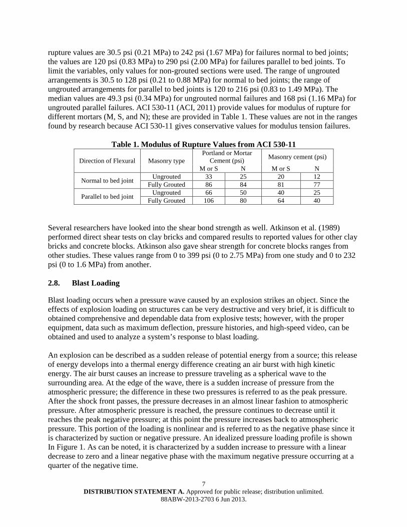
rupture values are 30.5 psi (0.21 MPa) to 242 psi (1.67 MPa) for failures normal to bed joints; the values are 120 psi (0.83 MPa) to 290 psi (2.00 MPa) for failures parallel to bed joints. To limit the variables, only values for non-grouted sections were used. The range of ungrouted arrangements is 30.5 to 128 psi (0.21 to 0.88 MPa) for normal to bed joints; the range of ungrouted arrangements for parallel to bed joints is 120 to 216 psi (0.83 to 1.49 MPa). The median values are 49.3 psi (0.34 MPa) for ungrouted normal failures and 168 psi (1.16 MPa) for ungrouted parallel failures. ACI 530-11 (ACI, 2011) provide values for modulus of rupture for different mortars (M, S, and N); these are provided in Table 1. These values are not in the ranges found by research because ACI 530-11 gives conservative values for modulus tension failures.
Table 1. Modulus of Rupture Values from ACI 530-11
Direction of Flexural Masonry type Portland or Mortar
Cement (psi) Masonry cement (psi)
M or S N M or S N
Normal to bed joint Ungrouted 33 25 20 12 Fully Grouted 86 84 81 77
Parallel to bed joint Ungrouted 66 50 40 25 Fully Grouted 106 80 64 40
Several researchers have looked into the shear bond strength as well. Atkinson et al. (1989) performed direct shear tests on clay bricks and compared results to reported values for other clay bricks and concrete blocks. Atkinson also gave shear strength for concrete blocks ranges from other studies. These values range from 0 to 399 psi (0 to 2.75 MPa) from one study and 0 to 232 psi (0 to 1.6 MPa) from another. 2.8. Blast Loading
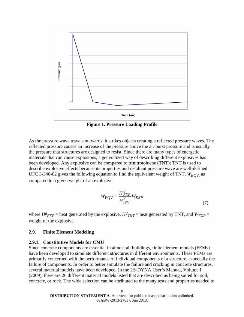
Blast loading occurs when a pressure wave caused by an explosion strikes an object. Since the effects of explosion loading on structures can be very destructive and very brief, it is difficult to obtained comprehensive and dependable data from explosive tests; however, with the proper equipment, data such as maximum deflection, pressure histories, and high-speed video, can be obtained and used to analyze a system’s response to blast loading. An explosion can be described as a sudden release of potential energy from a source; this release of energy develops into a thermal energy difference creating an air burst with high kinetic energy. The air burst causes an increase to pressure traveling as a spherical wave to the surrounding area. At the edge of the wave, there is a sudden increase of pressure from the atmospheric pressure; the difference in these two pressures is referred to as the peak pressure. After the shock front passes, the pressure decreases in an almost linear fashion to atmospheric pressure. After atmospheric pressure is reached, the pressure continues to decrease until it reaches the peak negative pressure; at this point the pressure increases back to atmospheric pressure. This portion of the loading is nonlinear and is referred to as the negative phase since it is characterized by suction or negative pressure. An idealized pressure loading profile is shown In Figure 1. As can be noted, it is characterized by a sudden increase to pressure with a linear decrease to zero and a linear negative phase with the maximum negative pressure occurring at a quarter of the negative time.
8 DISTRIBUTION STATEMENT A. Approved for public release; distribution unlimited.
88ABW-2013-2703 6 Jun 2013.
-25
0
25
50
75
100
125
150
175
200
225
0 10 20 30 40 50 60 70 80 90 100
Time (ms)
Pres
sure
(psi)
Figure 1. Pressure Loading Profile
As the pressure wave travels outwards, it strikes objects creating a reflected pressure waves. The reflected pressure causes an increase of the pressure above the air burst pressure and is usually the pressure that structures are designed to resist. Since there are many types of energetic materials that can cause explosions, a generalized way of describing different explosives has been developed. Any explosive can be compared to trinitrotoluene (TNT); TNT is used to describe explosive effects because its properties and resultant pressure wave are well-defined. UFC 3-340-02 gives the following equation to find the equivalent weight of TNT, WEQV, as compared to a given weight of an explosive.
dEXP
EQV EXPdTNT
HW WH
= (7)
where HdEXP = heat generated by the explosive, HdTNT = heat generated by TNT, and WEXP = weight of the explosive. 2.9. Finite Element Modeling
2.9.1. Constitutive Models for CMU Since concrete components are essential in almost all buildings, finite element models (FEMs) have been developed to simulate different structures in different environments. These FEMs are primarily concerned with the performance of individual components of a structure, especially the failure of components. In order to better simulate the failure and cracking in concrete structures, several material models have been developed. In the LS-DYNA User’s Manual, Volume I (2009), there are 26 different material models listed that are described as being suited for soil, concrete, or rock. The wide selection can be attributed to the many tests and properties needed to
9 DISTRIBUTION STATEMENT A. Approved for public release; distribution unlimited.
88ABW-2013-2703 6 Jun 2013.
define the behavior of concrete. Also, several models have been developed to help modelers by providing simple inputs and parameter generation algorithms. Davidson and Moradi (2008) looked at five material models (Soil and Foam, Soil and Foam with Failure, Brittle Damage, Pseudo Tensor, and Winfrith Concrete) in order to find the best model for CMU subjected to blast. In order to evaluate these models, a blast test was set up with single blocks at various standoff distances. The results were compared to finite element simulations ran in LS-DYNA. It was concluded that the Soil and Foam model best matched the test. Magallanes et al. (2010) mentioned that CMU acts like lightweight concrete and stated that the LS-DYNA material model Concrete Damage Release 3 “can provide excellent results if properly calibrated for these materials.” Very few others have looked directly at modeling and determining the best model for CMU. 2.9.2. CMU Models While there is little information on constitutive models for CMU, there is significantly more information on performing finite element modeling of CMU. Most of the work focuses exclusively on modeling walls. Martini (1997) developed a one-way masonry wall model to help in the investigation of rebuilding of Pompeii following an earthquake in 62 A.D. He proposed a block-interface model where the mortar is not modeled, but the interface between blocks retains the failure condition of the mortar. This model matched well with works published on static tests of one-way walls. Martini (1998) used the same block-interface model to simulate two-way bending of masonry walls. The results showed that as wall deflection increases, the reaction changes from the base carrying almost all the reactions to the base only carrying vertical reactions and the side supports carrying lateral reactions. He also observed that the blocks created moment couples along the edges. Finally, he noted that the failure pattern matched well with yield line pattern of the reinforced concrete slabs and created a method to apply the yield line analysis for masonry walls. Dennis et al. (2002) developed a CMU model of a single strip of blocks in the vertical direction. He used both quasi-static pressure test and dynamic blast test to verify the model taking into account maximum out-of-plane deflection and failure analysis; the results were slightly conservative and were unable to accurately predict all failures. Eamon et al. (2004) developed a model similar to the one by Dennis et al.; however, his was able to accurately predict the failure modes. Their work showed that there were three different failure modes for out-of-plane bending, (1) two-segment arching with the block remaining intact at low pressures, (2) two-segment arching with increased deflection and boundary block rotation leading to failure at medium pressures; and (3) multiple segments being expelled from the wall at various velocities at high pressure. The model also showed sensitivity to the material parameters; however, a change in failure type and a change in explosion loading velocity were relatively insensitive to material parameters. Burnett et al. (2006) performed finite element modeling on CMU walls subjected to low-velocity impacts. They described the creation of a discrete-crack model that employed tied interface
10 DISTRIBUTION STATEMENT A. Approved for public release; distribution unlimited.
88ABW-2013-2703 6 Jun 2013.
contact definition with normal and shear interface failure stresses, dilatant friction, gravity loads, and viscous hourglass control. They used a Mohr-Coulomb failure surface in the compression zone and a hemispherical cap in the tension zone. The investigation looked at impacts of a steel plate on CMU and brick walls and was used to determine wall failure modes, maximum displacement, and the influence of bonding pattern. Browning (2008) modeled multi-wythe walls that were fully grouted and had a brick veneer filled with a foam insulated cavity. He simulated the grout and CMU with a single smeared property based on the ratio of the area of grout to CMU. The brick veneer was not modeled discretely, but its mass was included in the model. Using the model, he developed engineering-level equations for out-of-plane bending using single degree-of-freedom (SDOF) and multiple degree-of-freedom (MDOF) methods. In addition to conventional CMU modeling, there has been research into modeling CMU retrofits. Sudame (2004) developed a model for a CMU wall with a spray-on polymer retrofit attached to the interior side of the wall. In modeling the polymer, he used a hyperelastic material model, a tied contact definition with tension and shear failures stresses, and a rupture failure definition. He also used a tied interface for the mortar joint with failure stresses. His research included a parametric study. Moradi’s (2008) work is an extension of Sudame, however his main focus was the development of a resistance equation for flexure which takes into account the effects of the retrofit.
11 DISTRIBUTION STATEMENT A. Approved for public release; distribution unlimited.
88ABW-2013-2703 6 Jun 2013.
3. METHODS, ASSUMPTIONS, AND PROCEDURES
3.1. Overview
Since concrete masonry walls are nonlinear both in their geometry and their material properties, finite element modeling is a valuable tool for understanding the behavior of these structures. Finite element model development can be complicated; however, once the model has been validated, it can be used to efficiently perform a large number of virtual tests. Livermore Software Technology Corporation’s LS-DYNA was used for this research because it is an advanced, general-purpose solver with the ability to run nonlinear, dynamic analyses. In order to do the preprocessing and post-processing, LS-PrePost, also produced by Livermore Software Technology Corporation, was used because of its compatibility with LS-DYNA. Any specifics in the following sections are given for input into LS-DYNA; these can be modified to simulate CMU for any appropriate finite element program, but these details should be viewed only as input for this specific investigation and not as general instructions on how to model CMU walls subjected to blast loading. 3.2. Dynamic Testing Overview
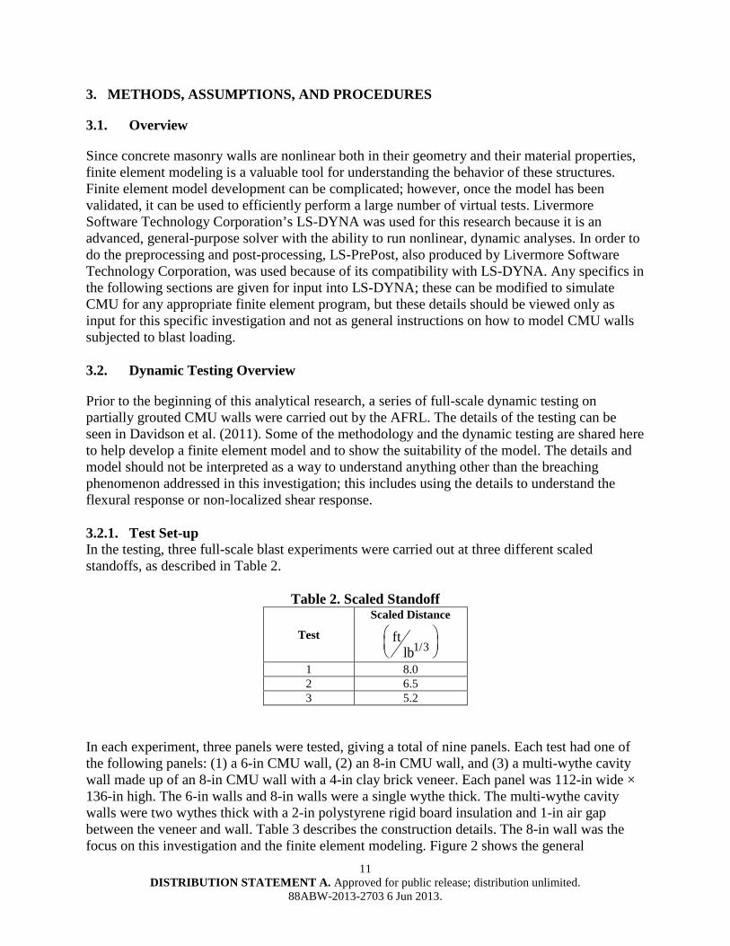
Prior to the beginning of this analytical research, a series of full-scale dynamic testing on partially grouted CMU walls were carried out by the AFRL. The details of the testing can be seen in Davidson et al. (2011). Some of the methodology and the dynamic testing are shared here to help develop a finite element model and to show the suitability of the model. The details and model should not be interpreted as a way to understand anything other than the breaching phenomenon addressed in this investigation; this includes using the details to understand the flexural response or non-localized shear response. 3.2.1. Test Set-up In the testing, three full-scale blast experiments were carried out at three different scaled standoffs, as described in Table 2.
Table 2. Scaled Standoff
Test
Scaled Distance
1/3ft
lb
1 8.0 2 6.5 3 5.2
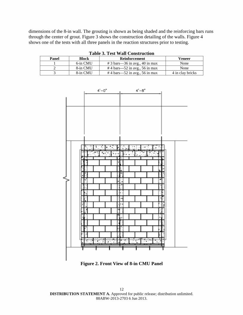
In each experiment, three panels were tested, giving a total of nine panels. Each test had one of the following panels: (1) a 6-in CMU wall, (2) an 8-in CMU wall, and (3) a multi-wythe cavity wall made up of an 8-in CMU wall with a 4-in clay brick veneer. Each panel was 112-in wide × 136-in high. The 6-in walls and 8-in walls were a single wythe thick. The multi-wythe cavity walls were two wythes thick with a 2-in polystyrene rigid board insulation and 1-in air gap between the veneer and wall. Table 3 describes the construction details. The 8-in wall was the focus on this investigation and the finite element modeling. Figure 2 shows the general
12 DISTRIBUTION STATEMENT A. Approved for public release; distribution unlimited.
88ABW-2013-2703 6 Jun 2013.
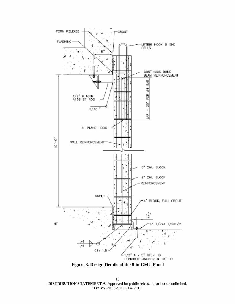
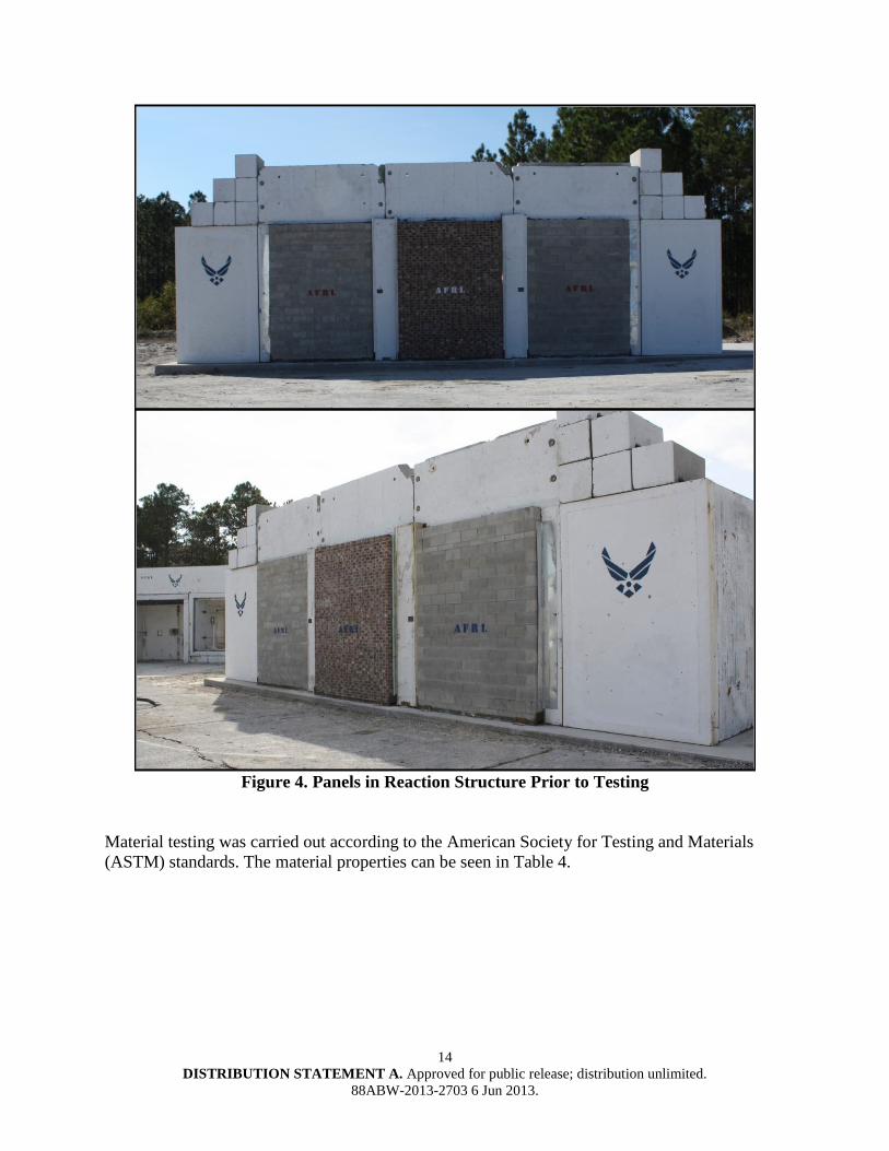
dimensions of the 8-in wall. The grouting is shown as being shaded and the reinforcing bars runs through the center of grout. Figure 3 shows the construction detailing of the walls. Figure 4 shows one of the tests with all three panels in the reaction structures prior to testing.
Table 3. Test Wall Construction Panel Block Reinforcement Veneer
1 6-in CMU # 3 bars—36 in avg., 40 in max None 2 8-in CMU # 4 bars—52 in avg., 56 in max None 3 8-in CMU # 4 bars—52 in avg., 56 in max 4 in clay bricks
Figure 2. Front View of 8-in CMU Panel
13 DISTRIBUTION STATEMENT A. Approved for public release; distribution unlimited.
88ABW-2013-2703 6 Jun 2013.
Figure 3. Design Details of the 8-in CMU Panel
14 DISTRIBUTION STATEMENT A. Approved for public release; distribution unlimited.
88ABW-2013-2703 6 Jun 2013.
Figure 4. Panels in Reaction Structure Prior to Testing
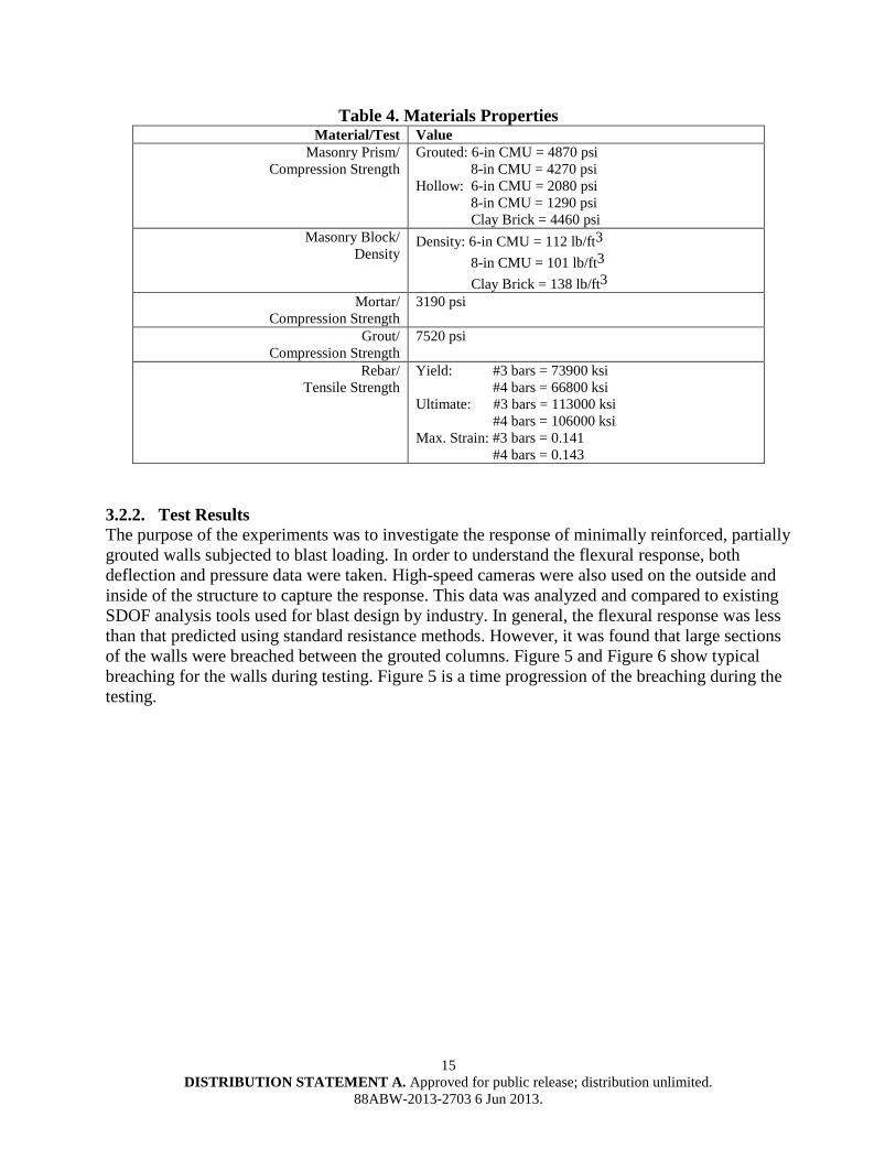
Material testing was carried out according to the American Society for Testing and Materials (ASTM) standards. The material properties can be seen in Table 4.
15 DISTRIBUTION STATEMENT A. Approved for public release; distribution unlimited.
88ABW-2013-2703 6 Jun 2013.
Table 4. Materials Properties Material/Test Value
Masonry Prism/ Compression Strength
Grouted: 6-in CMU = 4870 psi 8-in CMU = 4270 psi Hollow: 6-in CMU = 2080 psi 8-in CMU = 1290 psi Clay Brick = 4460 psi
Masonry Block/ Density
Density: 6-in CMU = 112 lb/ft3 8-in CMU = 101 lb/ft3 Clay Brick = 138 lb/ft3
Mortar/ Compression Strength
3190 psi
Grout/ Compression Strength
7520 psi
Rebar/ Tensile Strength
Yield: #3 bars = 73900 ksi #4 bars = 66800 ksi Ultimate: #3 bars = 113000 ksi #4 bars = 106000 ksi Max. Strain: #3 bars = 0.141 #4 bars = 0.143
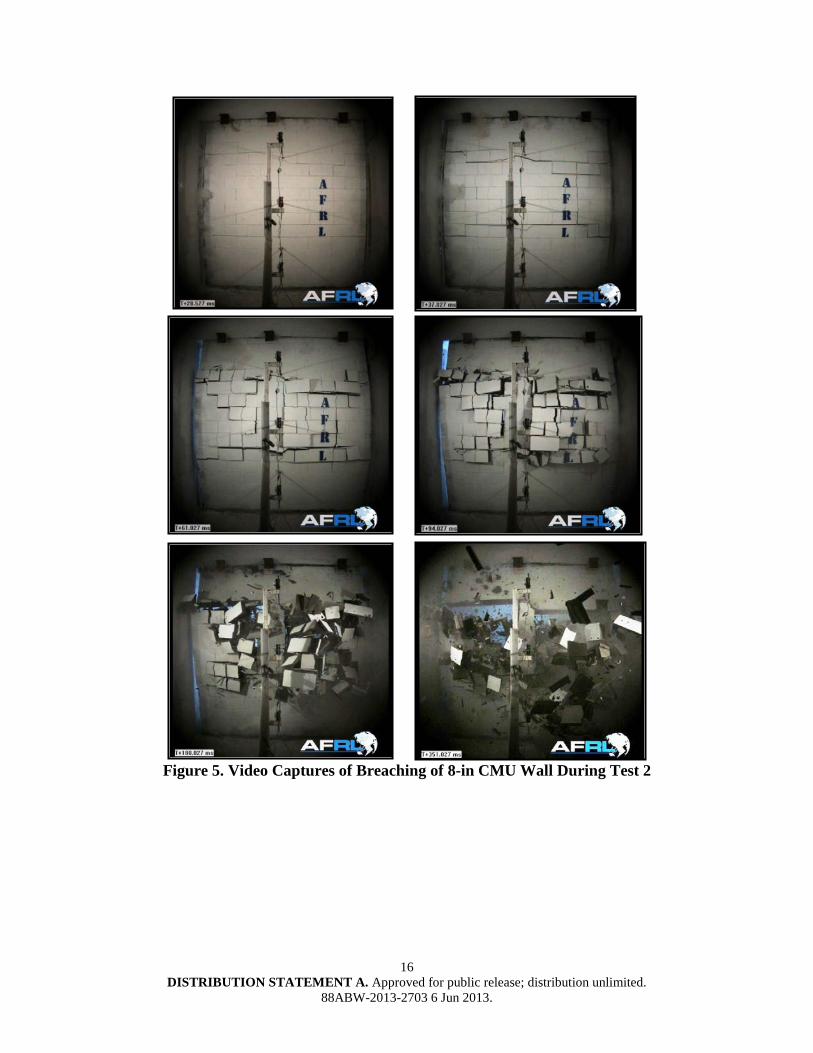
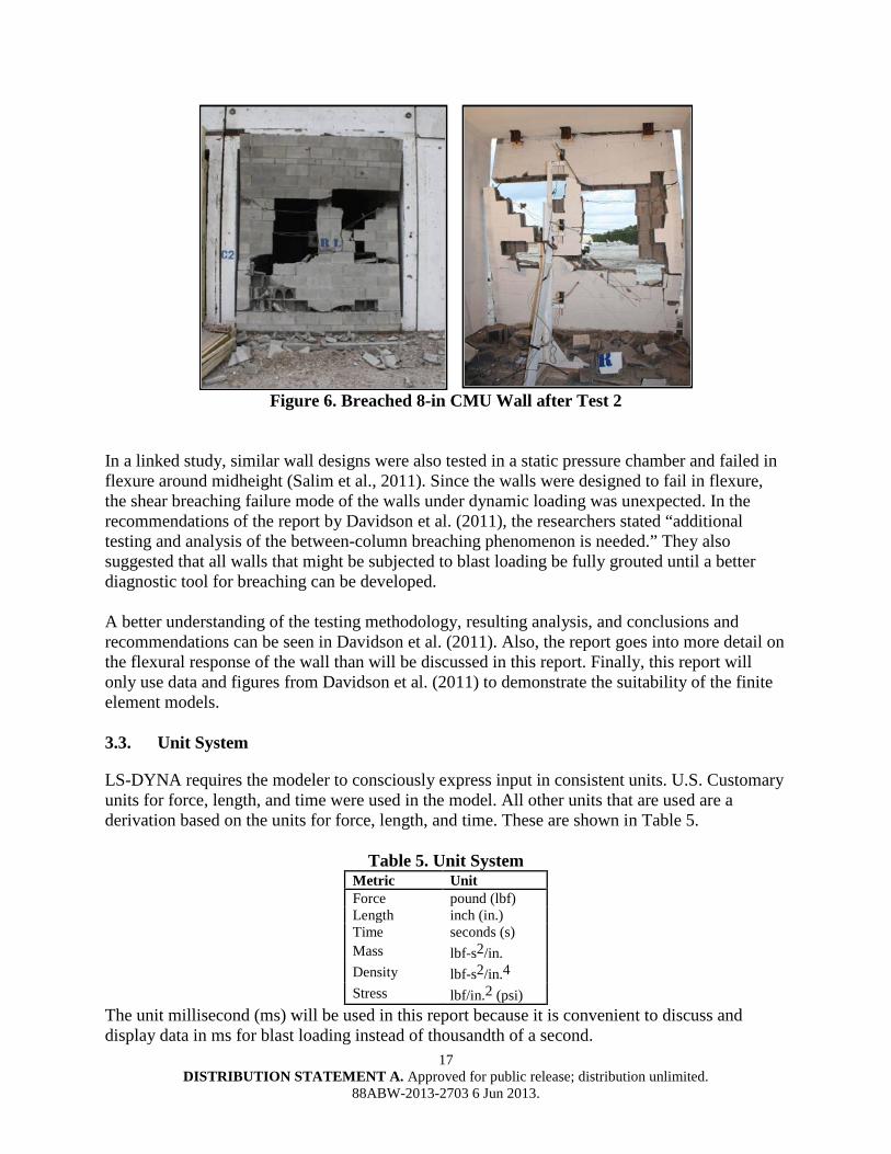
3.2.2. Test Results The purpose of the experiments was to investigate the response of minimally reinforced, partially grouted walls subjected to blast loading. In order to understand the flexural response, both deflection and pressure data were taken. High-speed cameras were also used on the outside and inside of the structure to capture the response. This data was analyzed and compared to existing SDOF analysis tools used for blast design by industry. In general, the flexural response was less than that predicted using standard resistance methods. However, it was found that large sections of the walls were breached between the grouted columns. Figure 5 and Figure 6 show typical breaching for the walls during testing. Figure 5 is a time progression of the breaching during the testing.
16 DISTRIBUTION STATEMENT A. Approved for public release; distribution unlimited.
88ABW-2013-2703 6 Jun 2013.
Figure 5. Video Captures of Breaching of 8-in CMU Wall During Test 2
17 DISTRIBUTION STATEMENT A. Approved for public release; distribution unlimited.
88ABW-2013-2703 6 Jun 2013.
Figure 6. Breached 8-in CMU Wall after Test 2
In a linked study, similar wall designs were also tested in a static pressure chamber and failed in flexure around midheight (Salim et al., 2011). Since the walls were designed to fail in flexure, the shear breaching failure mode of the walls under dynamic loading was unexpected. In the recommendations of the report by Davidson et al. (2011), the researchers stated “additional testing and analysis of the between-column breaching phenomenon is needed.” They also suggested that all walls that might be subjected to blast loading be fully grouted until a better diagnostic tool for breaching can be developed. A better understanding of the testing methodology, resulting analysis, and conclusions and recommendations can be seen in Davidson et al. (2011). Also, the report goes into more detail on the flexural response of the wall than will be discussed in this report. Finally, this report will only use data and figures from Davidson et al. (2011) to demonstrate the suitability of the finite element models. 3.3. Unit System
LS-DYNA requires the modeler to consciously express input in consistent units. U.S. Customary units for force, length, and time were used in the model. All other units that are used are a derivation based on the units for force, length, and time. These are shown in Table 5.
Table 5. Unit System Metric Unit Force pound (lbf) Length inch (in.) Time seconds (s) Mass lbf-s2/in. Density lbf-s2/in.4 Stress lbf/in.2 (psi)
The unit millisecond (ms) will be used in this report because it is convenient to discuss and display data in ms for blast loading instead of thousandth of a second.
18 DISTRIBUTION STATEMENT A. Approved for public release; distribution unlimited.
88ABW-2013-2703 6 Jun 2013.
3.4. Geometry and Meshing
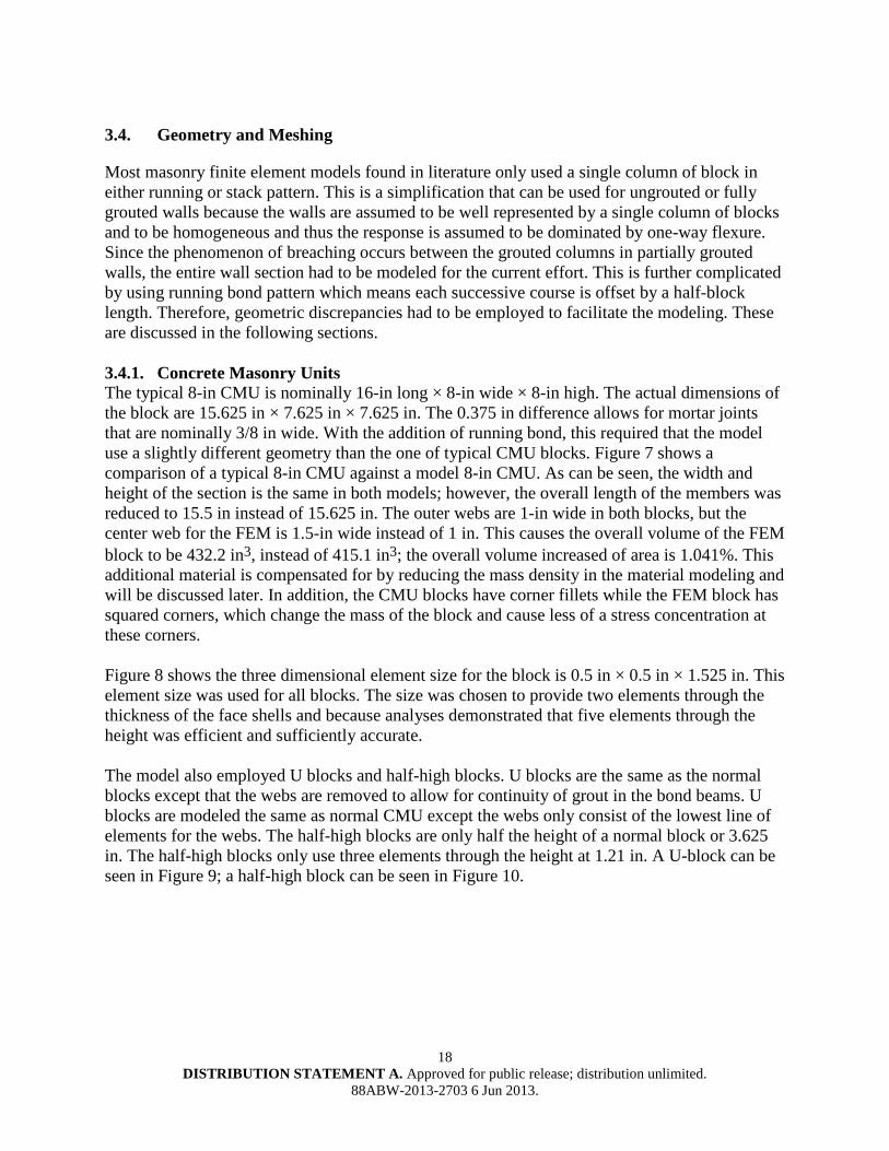
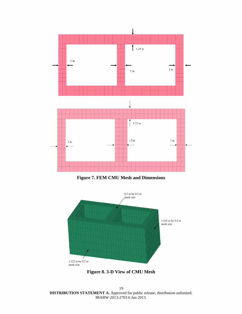
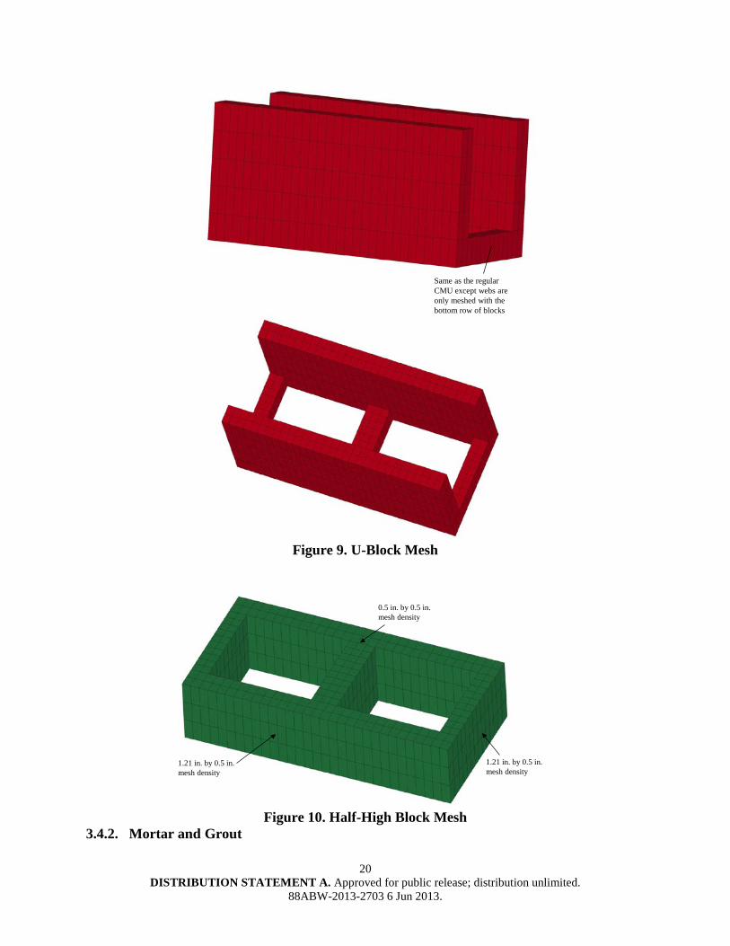
Most masonry finite element models found in literature only used a single column of block in either running or stack pattern. This is a simplification that can be used for ungrouted or fully grouted walls because the walls are assumed to be well represented by a single column of blocks and to be homogeneous and thus the response is assumed to be dominated by one-way flexure. Since the phenomenon of breaching occurs between the grouted columns in partially grouted walls, the entire wall section had to be modeled for the current effort. This is further complicated by using running bond pattern which means each successive course is offset by a half-block length. Therefore, geometric discrepancies had to be employed to facilitate the modeling. These are discussed in the following sections. 3.4.1. Concrete Masonry Units The typical 8-in CMU is nominally 16-in long × 8-in wide × 8-in high. The actual dimensions of the block are 15.625 in × 7.625 in × 7.625 in. The 0.375 in difference allows for mortar joints that are nominally 3/8 in wide. With the addition of running bond, this required that the model use a slightly different geometry than the one of typical CMU blocks. Figure 7 shows a comparison of a typical 8-in CMU against a model 8-in CMU. As can be seen, the width and height of the section is the same in both models; however, the overall length of the members was reduced to 15.5 in instead of 15.625 in. The outer webs are 1-in wide in both blocks, but the center web for the FEM is 1.5-in wide instead of 1 in. This causes the overall volume of the FEM block to be 432.2 in3, instead of 415.1 in3; the overall volume increased of area is 1.041%. This additional material is compensated for by reducing the mass density in the material modeling and will be discussed later. In addition, the CMU blocks have corner fillets while the FEM block has squared corners, which change the mass of the block and cause less of a stress concentration at these corners. Figure 8 shows the three dimensional element size for the block is 0.5 in × 0.5 in × 1.525 in. This element size was used for all blocks. The size was chosen to provide two elements through the thickness of the face shells and because analyses demonstrated that five elements through the height was efficient and sufficiently accurate. The model also employed U blocks and half-high blocks. U blocks are the same as the normal blocks except that the webs are removed to allow for continuity of grout in the bond beams. U blocks are modeled the same as normal CMU except the webs only consist of the lowest line of elements for the webs. The half-high blocks are only half the height of a normal block or 3.625 in. The half-high blocks only use three elements through the height at 1.21 in. A U-block can be seen in Figure 9; a half-high block can be seen in Figure 10.
19 DISTRIBUTION STATEMENT A. Approved for public release; distribution unlimited.
88ABW-2013-2703 6 Jun 2013.
Figure 7. FEM CMU Mesh and Dimensions
0.5 in by 0.5 in mesh size
1.525 in by 0.5 in mesh size
1.525 in by 0.5 in mesh size
Figure 8. 3-D View of CMU Mesh
20 DISTRIBUTION STATEMENT A. Approved for public release; distribution unlimited.
88ABW-2013-2703 6 Jun 2013.
Same as the regular CMU except webs are only meshed with the bottom row of blocks
Figure 9. U-Block Mesh
0.5 in. by 0.5 in. mesh density
1.21 in. by 0.5 in. mesh density
1.21 in. by 0.5 in. mesh density
Figure 10. Half-High Block Mesh
3.4.2. Mortar and Grout
21 DISTRIBUTION STATEMENT A. Approved for public release; distribution unlimited.
88ABW-2013-2703 6 Jun 2013.
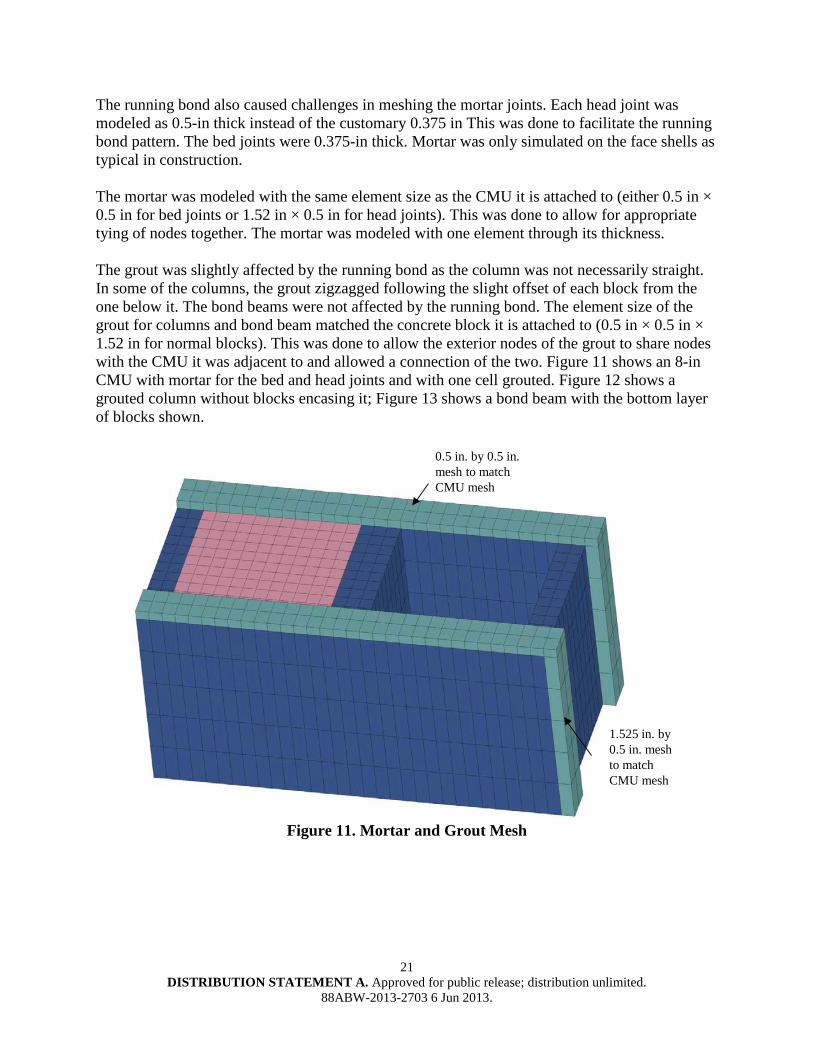
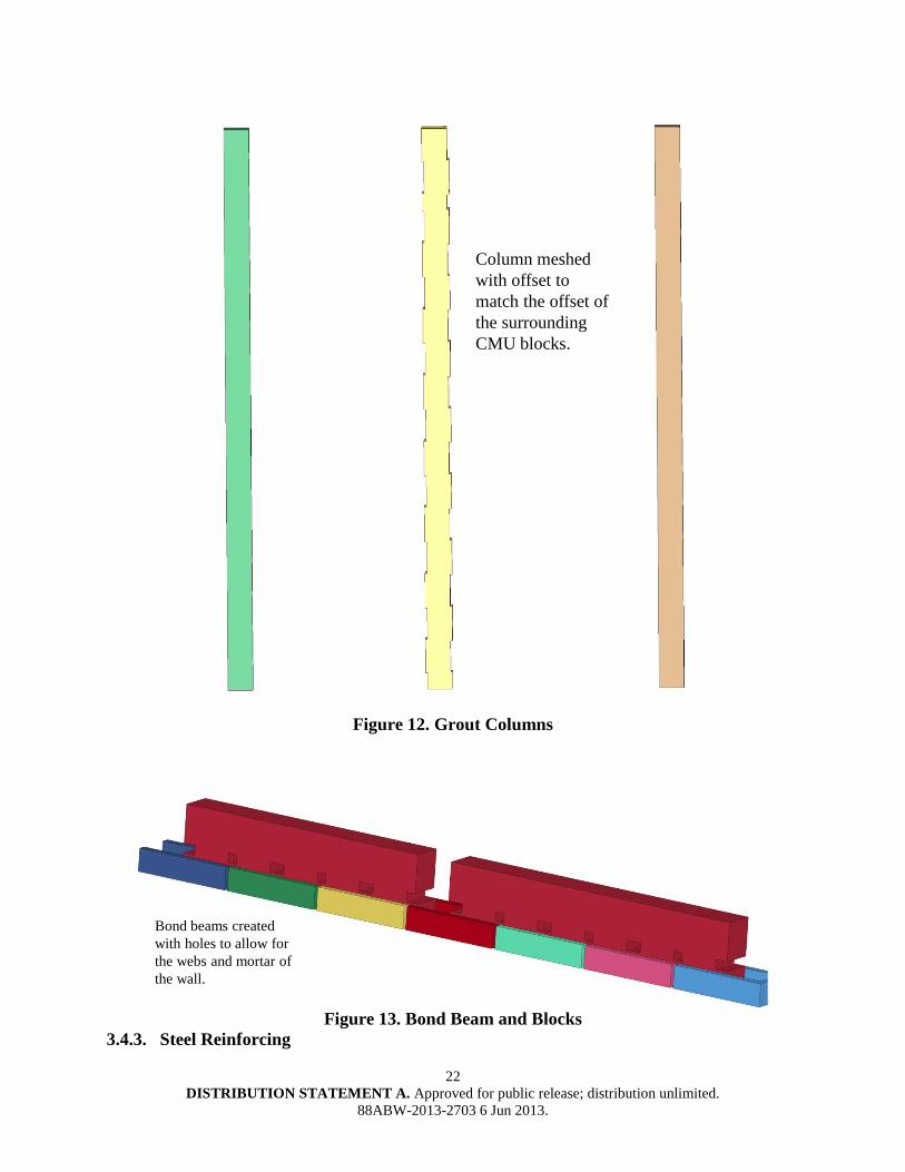
The running bond also caused challenges in meshing the mortar joints. Each head joint was modeled as 0.5-in thick instead of the customary 0.375 in This was done to facilitate the running bond pattern. The bed joints were 0.375-in thick. Mortar was only simulated on the face shells as typical in construction. The mortar was modeled with the same element size as the CMU it is attached to (either 0.5 in × 0.5 in for bed joints or 1.52 in × 0.5 in for head joints). This was done to allow for appropriate tying of nodes together. The mortar was modeled with one element through its thickness. The grout was slightly affected by the running bond as the column was not necessarily straight. In some of the columns, the grout zigzagged following the slight offset of each block from the one below it. The bond beams were not affected by the running bond. The element size of the grout for columns and bond beam matched the concrete block it is attached to (0.5 in × 0.5 in × 1.52 in for normal blocks). This was done to allow the exterior nodes of the grout to share nodes with the CMU it was adjacent to and allowed a connection of the two. Figure 11 shows an 8-in CMU with mortar for the bed and head joints and with one cell grouted. Figure 12 shows a grouted column without blocks encasing it; Figure 13 shows a bond beam with the bottom layer of blocks shown.
0.5 in. by 0.5 in. mesh to match CMU mesh
1.525 in. by 0.5 in. mesh to match CMU mesh
Figure 11. Mortar and Grout Mesh
22 DISTRIBUTION STATEMENT A. Approved for public release; distribution unlimited.
88ABW-2013-2703 6 Jun 2013.
Column meshed with offset to match the offset of the surrounding CMU blocks.
Figure 12. Grout Columns
Bond beams created with holes to allow for the webs and mortar of the wall.
Figure 13. Bond Beam and Blocks
3.4.3. Steel Reinforcing
23 DISTRIBUTION STATEMENT A. Approved for public release; distribution unlimited.
88ABW-2013-2703 6 Jun 2013.
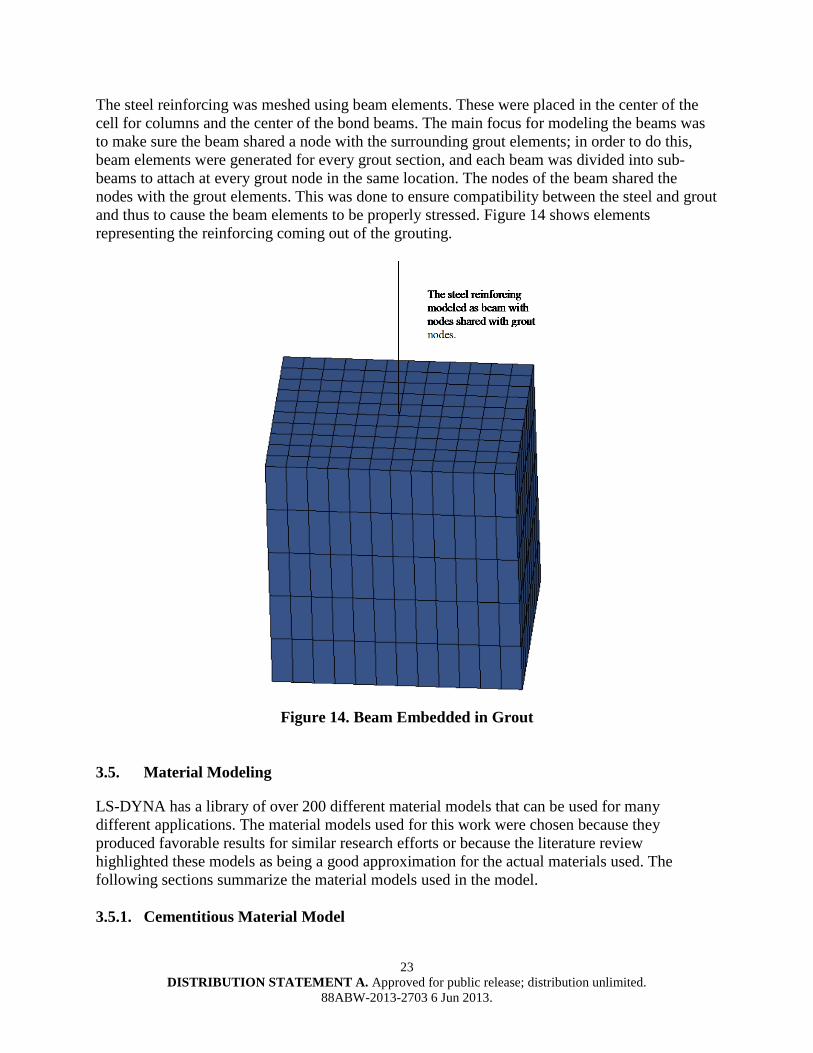
The steel reinforcing was meshed using beam elements. These were placed in the center of the cell for columns and the center of the bond beams. The main focus for modeling the beams was to make sure the beam shared a node with the surrounding grout elements; in order to do this, beam elements were generated for every grout section, and each beam was divided into sub-beams to attach at every grout node in the same location. The nodes of the beam shared the nodes with the grout elements. This was done to ensure compatibility between the steel and grout and thus to cause the beam elements to be properly stressed. Figure 14 shows elements representing the reinforcing coming out of the grouting.
Figure 14. Beam Embedded in Grout
3.5. Material Modeling
LS-DYNA has a library of over 200 different material models that can be used for many different applications. The material models used for this work were chosen because they produced favorable results for similar research efforts or because the literature review highlighted these models as being a good approximation for the actual materials used. The following sections summarize the material models used in the model. 3.5.1. Cementitious Material Model
24 DISTRIBUTION STATEMENT A. Approved for public release; distribution unlimited.
88ABW-2013-2703 6 Jun 2013.
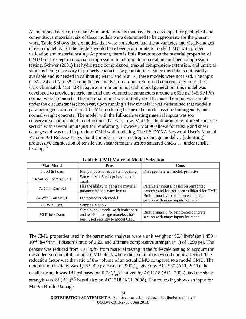
As mentioned earlier, there are 26 material models that have been developed for geological and cementitious materials; six of these models were determined to be appropriate for the present work. Table 6 shows the six models that were considered and the advantages and disadvantages of each model. All of the models would have been appropriate to model CMU with proper validation and material testing. At present, there is little literature on the material properties of CMU block except in uniaxial compression. In addition to uniaxial, unconfined compression testing, Schwer (2001) list hydrostatic compression, triaxial compression/extension, and uniaxial strain as being necessary to properly characterize geomaterials. Since this data is not readily available and is needed in calibrating Mat 5 and Mat 14, these models were not used. The input of Mat 84 and Mat 85 is complicated and is built around reinforced concrete; therefore, these were eliminated. Mat 72R3 requires minimum input with model generation; this model was developed to provide generic material and volumetric parameters around a 6610 psi (45.6 MPa) normal weight concrete. This material model was initially used because the input was simple under the circumstances; however, upon running a few models it was determined that model’s parameter generation did not fit CMU modeling because the model assume homogeneity and normal weight concrete. The model with the full-scale testing material inputs was too conservative and resulted in deflections that were low. Mat 96 is built around reinforced concrete section with several inputs just for reinforcing. However, Mat 96 allows for tensile and shear damage and was used in previous CMU wall modeling. The LS-DYNA Keyword User’s Manual Version 971 Release 4 says that the model is “an anisotropic damage model … [admitting] progressive degradation of tensile and shear strengths across smeared cracks … under tensile loadings.”
Table 6. CMU Material Model Selection Mat. Model Pros Cons
5 Soil & Foam Many inputs for accurate modeling First geomaterial model; primitive
14 Soil & Foam w/ Fail. Same as Mat 5 except has tension cutoff
72 Con. Dam R3 Has the ability to generate material parameters; has many inputs
Parameter input is based on reinforced concrete and has not been validated for CMU
84 Win. Con w/ RE Is smeared crack model Built primarily for reinforced concrete section with many inputs for rebar
85 Win. Con. Same as Mat 85
96 Brittle Dam. Simple input model with both shear and tension damage modeled; has been used recently to model CMU.
Built primarily for reinforced concrete section with many inputs for rebar
The CMU properties used in the parametric analyses were a unit weight of 96.8 lb/ft3 (or 1.450 × 10⁻⁴ lb-s2/in4), Poisson’s ratio of 0.20, and ultimate compressive strength (f’m) of 1290 psi. The density was reduced from 101 lb/ft3 from material testing in the full-scale testing to account for the added volume of the model CMU block where the overall mass would not be affected. The reduction factor was the ratio of the volume of an actual CMU compared to a model CMU. The modulus of elasticity was 1,163,000 psi based on 900 f’m given by ACI 530 (ACI, 2011), the tensile strength was 181 psi based on 6.7λ(f’m)0.5 given by ACI 318 (ACI, 2008), and the shear strength was 2λ ( f’m)0.5 based also on ACI 318 (ACI, 2008). The following shows an input for Mat 96 Brittle Damage.
25 DISTRIBUTION STATEMENT A. Approved for public release; distribution unlimited.
88ABW-2013-2703 6 Jun 2013.
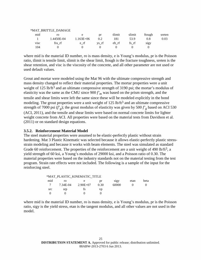
*MAT_BRITTLE_DAMAGE mid ro e pr tlimit slimit ftough sreten 1 1.4450E-04 1.163E+06 0.2 181 53.9 0.8 0.03 visc fra_rf e_rf ys_rf eh_rf fs_rf sigy 104 0 0 0 0 0 0
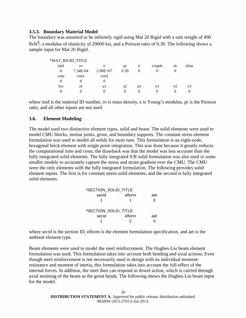
where mid is the material ID number, ro is mass density, e is Young’s modulus, pr is the Poisson ratio, tlimit is tensile limit, slimit is the shear limit, ftough is the fracture toughness, sreten is the shear retention, and visc is the viscosity of the concrete, and all other parameter are not used or used default values. Grout and mortar were modeled using the Mat 96 with the ultimate compressive strength and mass density changed to reflect their material properties. The mortar properties were a unit weight of 125 lb/ft3 and an ultimate compressive strength of 3190 psi; the mortar’s modulus of elasticity was the same as the CMU since 900 f’m was based on the prism strength, and the tensile and shear limits were left the same since these will be modeled explicitly in the bond modeling. The grout properties were a unit weight of 125 lb/ft3 and an ultimate compressive strength of 7000 psi (f’g); the grout modulus of elasticity was given by 500 f’g based on ACI 530 (ACI, 2011), and the tensile and shear limits were based on normal concrete limits for lighter weight concrete from ACI. All properties were based on the material tests from Davidson et al. (2011) or on standard design equations. 3.5.2. Reinforcement Material Model The steel material properties were assumed to be elastic-perfectly plastic without strain hardening. Mat 3 Plastic Kinematic was selected because it allows elastic-perfectly plastic stress-strain modeling and because it works with beam elements. The steel was simulated as standard Grade 60 reinforcement. The properties of the reinforcement are a unit weight of 490 lb/ft3, a yield strength of 60 ksi, a Young’s modulus of 29000 ksi, and a Poisson ratio of 0.30. The material properties were based on the industry standards not on the material testing from the test program. Strain rate effects were not included. The following is a sample of the input for the reinforcing steel.
*MAT_PLASTIC_KINEMATIC_TITLE mid ro e pr sigy etan beta
7 7.34E-04 2.90E+07 0.30 60000 0 0 src srp fs vp 0 0 0 0
where mid is the material ID number, ro is mass density, e is Young’s modulus, pr is the Poisson ratio, sigy is the yield stress, etan is the tangent modulus, and all other values are not used in the model.
26 DISTRIBUTION STATEMENT A. Approved for public release; distribution unlimited.
88ABW-2013-2703 6 Jun 2013.
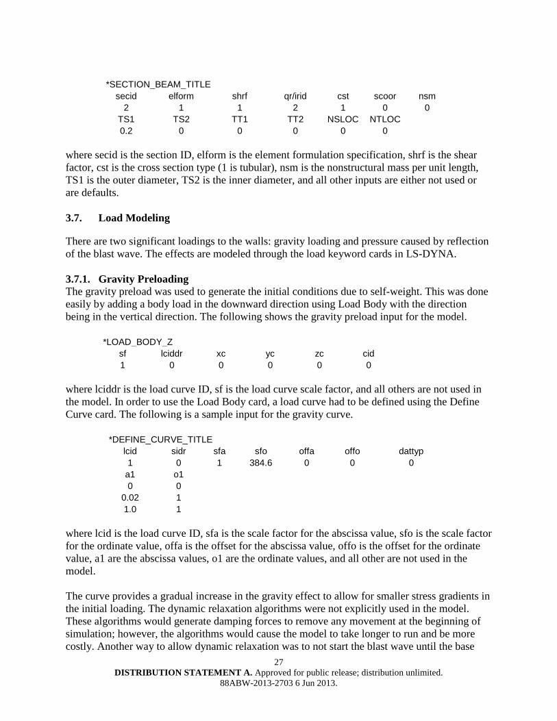
3.5.3. Boundary Material Model The boundary was assumed to be infinitely rigid using Mat 20 Rigid with a unit weight of 490 lb/ft3, a modulus of elasticity of 29000 ksi, and a Poisson ratio of 0.30. The following shows a sample input for Mat 20 Rigid.
*MAT_RIGID_TITLE mid ro e pr n couple m alias 6 7.34E-04 2.90E+07 0.30 0 0 0 cmo con1 con2 0 0 0 lco or a1 a2 a3 v1 v2 v3 0 0 0 0 0 0 0 0
where mid is the material ID number, ro is mass density, e is Young’s modulus, pr is the Poisson ratio, and all other inputs are not used. 3.6. Element Modeling
The model used two distinctive element types, solid and beam. The solid elements were used to model CMU blocks, mortar joints, grout, and boundary supports. The constant stress element formulation was used to model all solids for most runs. This formulation is an eight-node, hexagonal brick element with single point integration. This was done because it greatly reduces the computational time and costs; the drawback was that the model was less accurate than the fully integrated solid elements. The fully integrated S/R solid formulation was also used in some smaller models to accurately capture the stress and strain gradient over the CMU. The CMU were the only elements with the fully integrated formulation. The following provides solid element inputs. The first is for constant stress solid elements, and the second is fully integrated solid elements.
*SECTION_SOLID_TITLE secid elform aet 1 1 0
*SECTION_SOLID_TITLE secid elform aet 1 2 0
where secid is the section ID, elform is the element formulation specification, and aet is the ambient element type. Beam elements were used to model the steel reinforcement. The Hughes-Liu beam element formulation was used. This formulation takes into account both bending and axial actions. Even though steel reinforcement is not necessarily used in design with its individual moment-resistance and moment of inertia, this formulation takes into account the full-effect of the internal forces. In addition, the steel then can respond in dowel action, which is carried through axial straining of the beam as the grout bends. The following shows the Hughes-Liu beam input for the model.
27 DISTRIBUTION STATEMENT A. Approved for public release; distribution unlimited.
88ABW-2013-2703 6 Jun 2013.
*SECTION_BEAM_TITLE
secid elform shrf qr/irid cst scoor nsm 2 1 1 2 1 0 0
TS1 TS2 TT1 TT2 NSLOC NTLOC 0.2 0 0 0 0 0
where secid is the section ID, elform is the element formulation specification, shrf is the shear factor, cst is the cross section type (1 is tubular), nsm is the nonstructural mass per unit length, TS1 is the outer diameter, TS2 is the inner diameter, and all other inputs are either not used or are defaults. 3.7. Load Modeling
There are two significant loadings to the walls: gravity loading and pressure caused by reflection of the blast wave. The effects are modeled through the load keyword cards in LS-DYNA. 3.7.1. Gravity Preloading The gravity preload was used to generate the initial conditions due to self-weight. This was done easily by adding a body load in the downward direction using Load Body with the direction being in the vertical direction. The following shows the gravity preload input for the model.
*LOAD_BODY_Z sf lciddr xc yc zc cid 1 0 0 0 0 0
where lciddr is the load curve ID, sf is the load curve scale factor, and all others are not used in the model. In order to use the Load Body card, a load curve had to be defined using the Define Curve card. The following is a sample input for the gravity curve.
*DEFINE_CURVE_TITLE lcid sidr sfa sfo offa offo dattyp 1 0 1 384.6 0 0 0
a1 o1 0 0
0.02 1 1.0 1
where lcid is the load curve ID, sfa is the scale factor for the abscissa value, sfo is the scale factor for the ordinate value, offa is the offset for the abscissa value, offo is the offset for the ordinate value, a1 are the abscissa values, o1 are the ordinate values, and all other are not used in the model. The curve provides a gradual increase in the gravity effect to allow for smaller stress gradients in the initial loading. The dynamic relaxation algorithms were not explicitly used in the model. These algorithms would generate damping forces to remove any movement at the beginning of simulation; however, the algorithms would cause the model to take longer to run and be more costly. Another way to allow dynamic relaxation was to not start the blast wave until the base
28 DISTRIBUTION STATEMENT A. Approved for public release; distribution unlimited.
88ABW-2013-2703 6 Jun 2013.
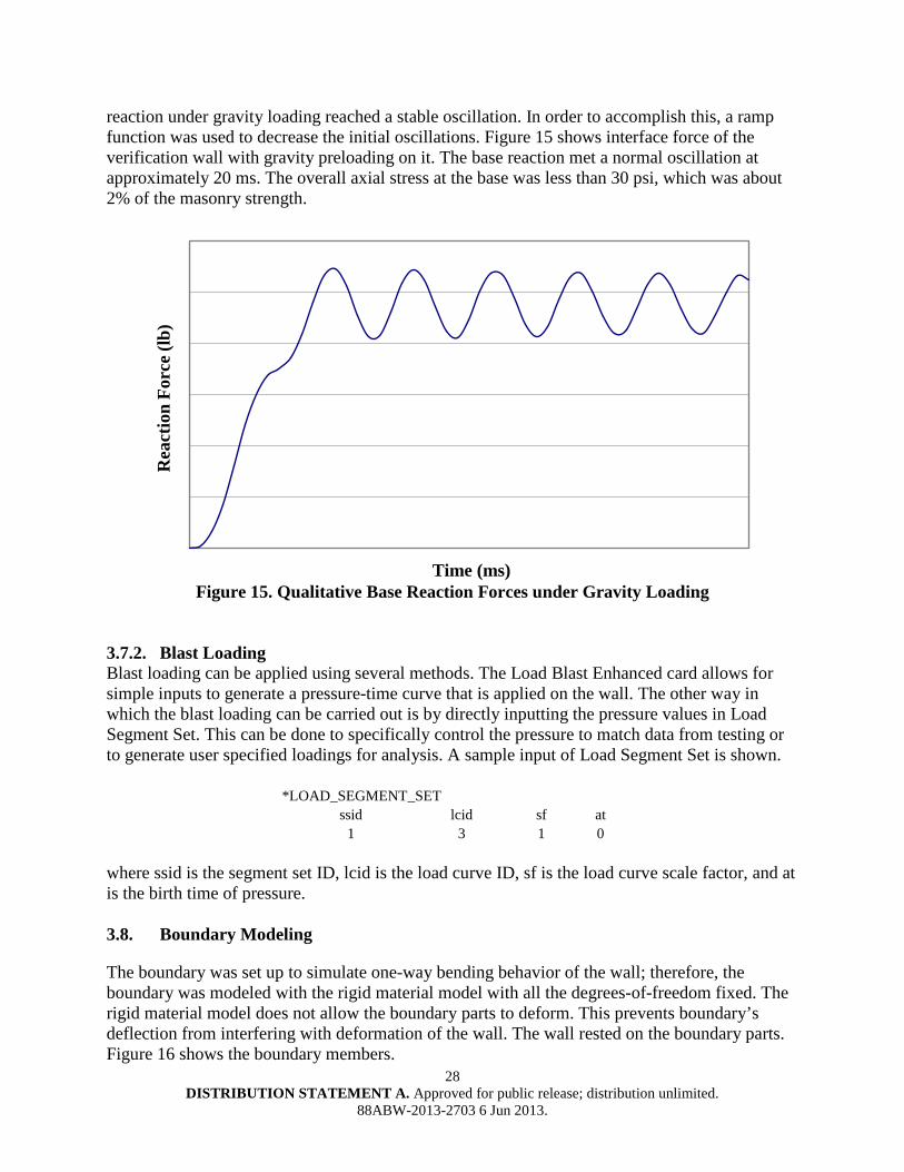
reaction under gravity loading reached a stable oscillation. In order to accomplish this, a ramp function was used to decrease the initial oscillations. Figure 15 shows interface force of the verification wall with gravity preloading on it. The base reaction met a normal oscillation at approximately 20 ms. The overall axial stress at the base was less than 30 psi, which was about 2% of the masonry strength.
Rea
ctio
n Fo
rce
(lb)
Time (ms) Figure 15. Qualitative Base Reaction Forces under Gravity Loading
3.7.2. Blast Loading Blast loading can be applied using several methods. The Load Blast Enhanced card allows for simple inputs to generate a pressure-time curve that is applied on the wall. The other way in which the blast loading can be carried out is by directly inputting the pressure values in Load Segment Set. This can be done to specifically control the pressure to match data from testing or to generate user specified loadings for analysis. A sample input of Load Segment Set is shown.
*LOAD_SEGMENT_SET ssid lcid sf at 1 3 1 0
where ssid is the segment set ID, lcid is the load curve ID, sf is the load curve scale factor, and at is the birth time of pressure. 3.8. Boundary Modeling
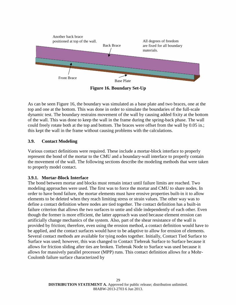
The boundary was set up to simulate one-way bending behavior of the wall; therefore, the boundary was modeled with the rigid material model with all the degrees-of-freedom fixed. The rigid material model does not allow the boundary parts to deform. This prevents boundary’s deflection from interfering with deformation of the wall. The wall rested on the boundary parts. Figure 16 shows the boundary members.
29 DISTRIBUTION STATEMENT A. Approved for public release; distribution unlimited.
88ABW-2013-2703 6 Jun 2013.
Front Brace
Back Brace
Base Plate
Another back brace positioned at top of the wall. All degrees of freedom
are fixed for all boundary materials.
Figure 16. Boundary Set-Up
As can be seen Figure 16, the boundary was simulated as a base plate and two braces, one at the top and one at the bottom. This was done in order to simulate the boundaries of the full-scale dynamic test. The boundary restrains movement of the wall by causing added fixity at the bottom of the wall. This was done to keep the wall in the frame during the spring-back phase. The wall could freely rotate both at the top and bottom. The braces were offset from the wall by 0.05 in.; this kept the wall in the frame without causing problems with the calculations. 3.9. Contact Modeling
Various contact definitions were required. These include a mortar-block interface to properly represent the bond of the mortar to the CMU and a boundary-wall interface to properly contain the movement of the wall. The following sections describe the modeling methods that were taken to properly model contact. 3.9.1. Mortar-Block Interface The bond between mortar and blocks must remain intact until failure limits are reached. Two modeling approaches were used. The first was to force the mortar and CMU to share nodes. In order to have bond failure, the mortar elements must have erosive properties built-in it to allow elements to be deleted when they reach limiting stress or strain values. The other way was to define a contact definition where nodes are tied together. The contact definition has a built-in failure criterion that allows the two surfaces to untie and slide independently of each other. Even though the former is more efficient, the latter approach was used because element erosion can artificially change mechanics of the system. Also, part of the shear resistance of the wall is provided by friction; therefore, even using the erosion method, a contact definition would have to be applied, and the contact surfaces would have to be adaptive to allow for erosion of elements. Several contact methods are available for tying nodes together. Initially, Contact Tied Surface to Surface was used; however, this was changed to Contact Tiebreak Surface to Surface because it allows for friction sliding after ties are broken. Tiebreak Node to Surface was used because it allows for massively parallel processor (MPP) runs. This contact definition allows for a Mohr-Coulomb failure surface characterized by
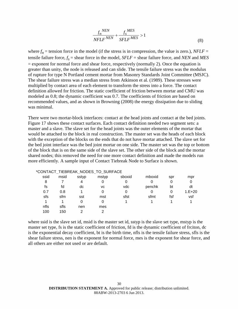
30 DISTRIBUTION STATEMENT A. Approved for public release; distribution unlimited.
88ABW-2013-2703 6 Jun 2013.
1
NEN MESn s
NEN MESf f
NFLF SFLF+ >
(8) where fn = tension force in the model (if the stress is in compression, the value is zero.), NFLF = tensile failure force, fs = shear force in the model, SFLF = shear failure force, and NEN and MES = exponent for normal force and shear force, respectively (normally 2). Once the equation is greater than unity, the node is released and can slide. The tensile failure stress was the modulus of rupture for type N Portland cement mortar from Masonry Standards Joint Committee (MSJC). The shear failure stress was a median stress from Atkinson et al. (1989). These stresses were multiplied by contact area of each element to transform the stress into a force. The contact definition allowed for friction. The static coefficient of friction between mortar and CMU was modeled as 0.8; the dynamic coefficient was 0.7. The coefficients of friction are based on recommended values, and as shown in Browning (2008) the energy dissipation due to sliding was minimal. There were two mortar-block interfaces: contact at the head joints and contact at the bed joints. Figure 17 shows these contact surfaces. Each contact definition needed two segment sets: a master and a slave. The slave set for the head joints was the outer elements of the mortar that would be attached to the block in real construction. The master set was the heads of each block with the exception of the blocks on the ends that do not have mortar attached. The slave set for the bed joint interface was the bed joint mortar on one side. The master set was the top or bottom of the block that is on the same side of the slave set. The other side of the block and the mortar shared nodes; this removed the need for one more contact definition and made the models run more efficiently. A sample input of Contact Tiebreak Node to Surface is shown.
*CONTACT_TIEBREAK_NODES_TO_SURFACE ssid msid sstyp mstyp sboxid mboxid spr mpr 8 7 4 0 0 0 0 0 fs fd dc vc vdc penchk bt dt 0.7 0.8 1 0 0 0 0 1.E+20 sfs sfm sst mst sfst sfmt fsf vsf 1 1 0 0 1 1 1 1 nfls sfls nen mes 100 150 2 2
where ssid is the slave set id, msid is the master set id, sstyp is the slave set type, mstyp is the master set type, fs is the static coefficient of friction, fd is the dynamic coefficient of frciton, dc is the exponential decay coefficient, bt is the birth time, nfls is the tensile failure stress, sfls is the shear failure stress, nen is the exponent for normal force, mes is the exponent for shear force, and all others are either not used or are default.
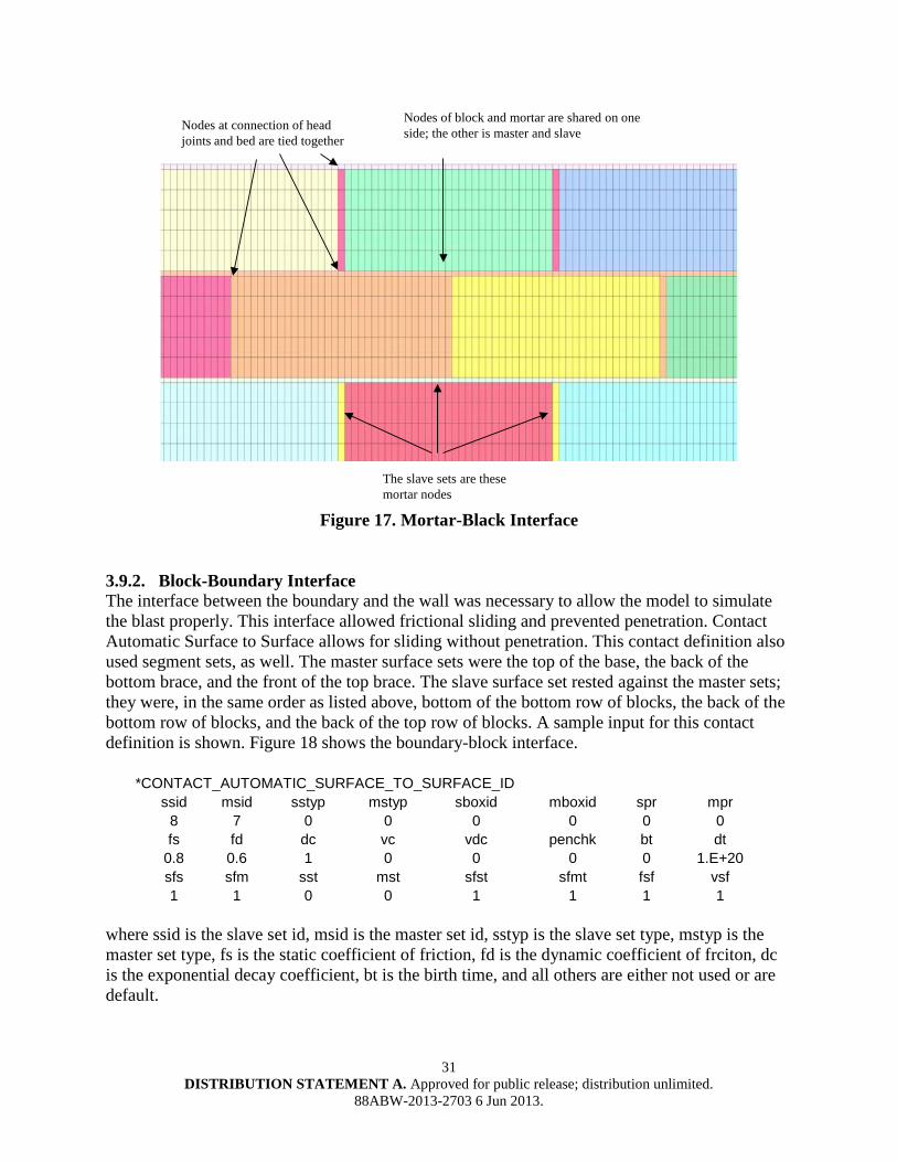
31 DISTRIBUTION STATEMENT A. Approved for public release; distribution unlimited.
88ABW-2013-2703 6 Jun 2013.
Nodes at connection of head joints and bed are tied together
Nodes of block and mortar are shared on one side; the other is master and slave
The slave sets are these mortar nodes
Figure 17. Mortar-Black Interface 3.9.2. Block-Boundary Interface The interface between the boundary and the wall was necessary to allow the model to simulate the blast properly. This interface allowed frictional sliding and prevented penetration. Contact Automatic Surface to Surface allows for sliding without penetration. This contact definition also used segment sets, as well. The master surface sets were the top of the base, the back of the bottom brace, and the front of the top brace. The slave surface set rested against the master sets; they were, in the same order as listed above, bottom of the bottom row of blocks, the back of the bottom row of blocks, and the back of the top row of blocks. A sample input for this contact definition is shown. Figure 18 shows the boundary-block interface.
*CONTACT_AUTOMATIC_SURFACE_TO_SURFACE_ID ssid msid sstyp mstyp sboxid mboxid spr mpr 8 7 0 0 0 0 0 0 fs fd dc vc vdc penchk bt dt 0.8 0.6 1 0 0 0 0 1.E+20 sfs sfm sst mst sfst sfmt fsf vsf 1 1 0 0 1 1 1 1
where ssid is the slave set id, msid is the master set id, sstyp is the slave set type, mstyp is the master set type, fs is the static coefficient of friction, fd is the dynamic coefficient of frciton, dc is the exponential decay coefficient, bt is the birth time, and all others are either not used or are default.
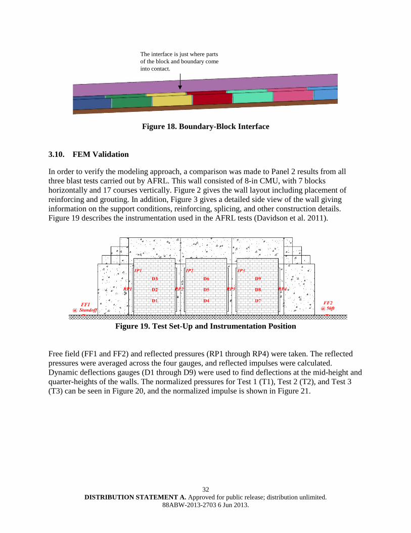
32 DISTRIBUTION STATEMENT A. Approved for public release; distribution unlimited.
88ABW-2013-2703 6 Jun 2013.
The interface is just where parts of the block and boundary come into contact.
Figure 18. Boundary-Block Interface
3.10. FEM Validation
In order to verify the modeling approach, a comparison was made to Panel 2 results from all three blast tests carried out by AFRL. This wall consisted of 8-in CMU, with 7 blocks horizontally and 17 courses vertically. Figure 2 gives the wall layout including placement of reinforcing and grouting. In addition, Figure 3 gives a detailed side view of the wall giving information on the support conditions, reinforcing, splicing, and other construction details. Figure 19 describes the instrumentation used in the AFRL tests (Davidson et al. 2011).
Figure 19. Test Set-Up and Instrumentation Position
Free field (FF1 and FF2) and reflected pressures (RP1 through RP4) were taken. The reflected pressures were averaged across the four gauges, and reflected impulses were calculated. Dynamic deflections gauges (D1 through D9) were used to find deflections at the mid-height and quarter-heights of the walls. The normalized pressures for Test 1 (T1), Test 2 (T2), and Test 3 (T3) can be seen in Figure 20, and the normalized impulse is shown in Figure 21.
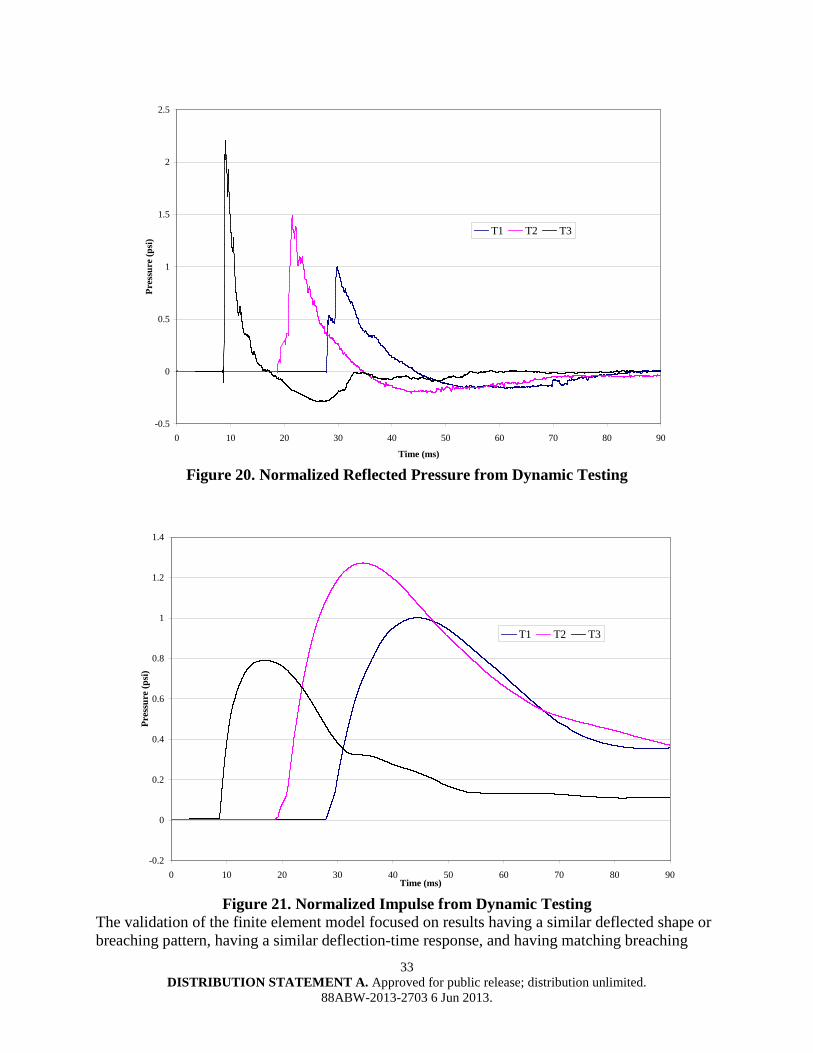
33 DISTRIBUTION STATEMENT A. Approved for public release; distribution unlimited.
88ABW-2013-2703 6 Jun 2013.
-0.5
0
0.5
1
1.5
2
2.5
0 10 20 30 40 50 60 70 80 90
Time (ms)
Pres
sure
(psi
)
T1 T2 T3
Figure 20. Normalized Reflected Pressure from Dynamic Testing
-0.2
0
0.2
0.4
0.6
0.8
1
1.2
1.4
0 10 20 30 40 50 60 70 80 90Time (ms)
Pres
sure
(psi
)
T1 T2 T3
Figure 21. Normalized Impulse from Dynamic Testing
The validation of the finite element model focused on results having a similar deflected shape or breaching pattern, having a similar deflection-time response, and having matching breaching
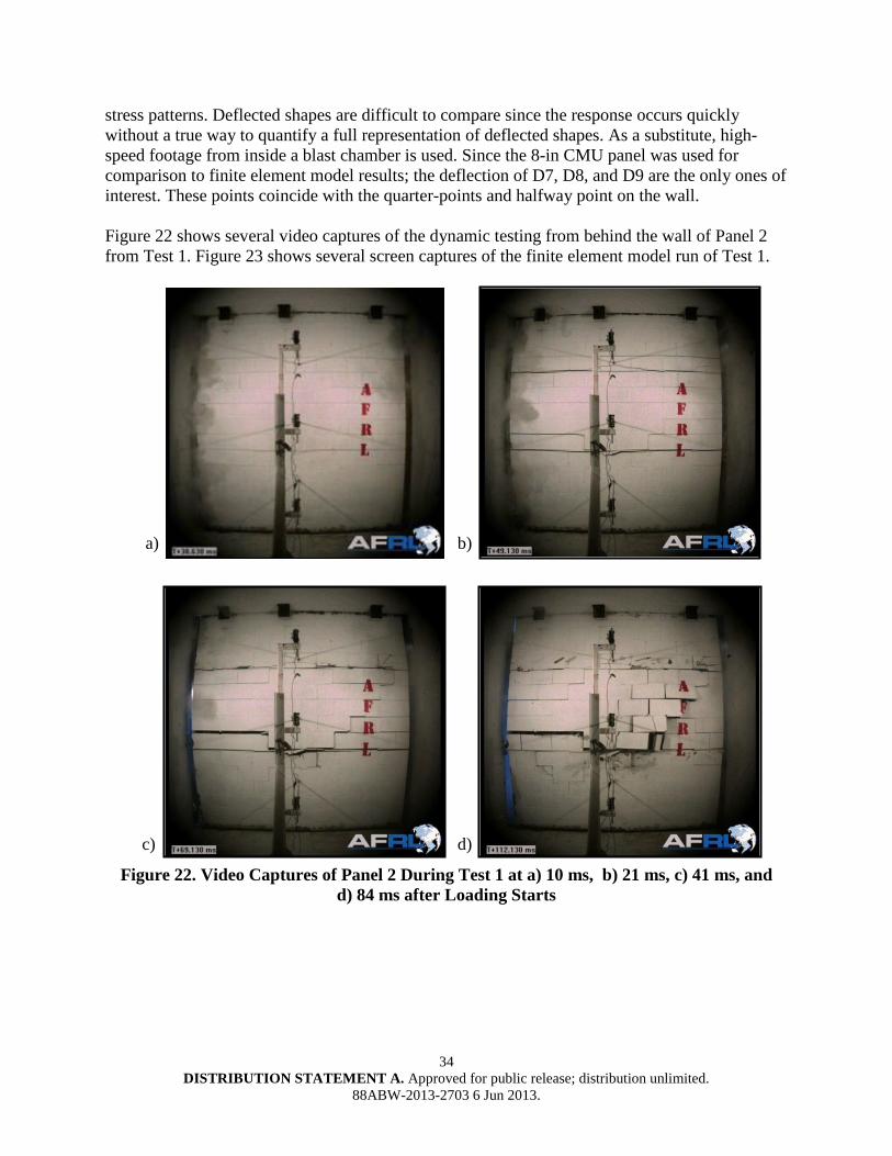
34 DISTRIBUTION STATEMENT A. Approved for public release; distribution unlimited.
88ABW-2013-2703 6 Jun 2013.
stress patterns. Deflected shapes are difficult to compare since the response occurs quickly without a true way to quantify a full representation of deflected shapes. As a substitute, high-speed footage from inside a blast chamber is used. Since the 8-in CMU panel was used for comparison to finite element model results; the deflection of D7, D8, and D9 are the only ones of interest. These points coincide with the quarter-points and halfway point on the wall. Figure 22 shows several video captures of the dynamic testing from behind the wall of Panel 2 from Test 1. Figure 23 shows several screen captures of the finite element model run of Test 1.
a)
c)
b)
d)
Figure 22. Video Captures of Panel 2 During Test 1 at a) 10 ms, b) 21 ms, c) 41 ms, and d) 84 ms after Loading Starts
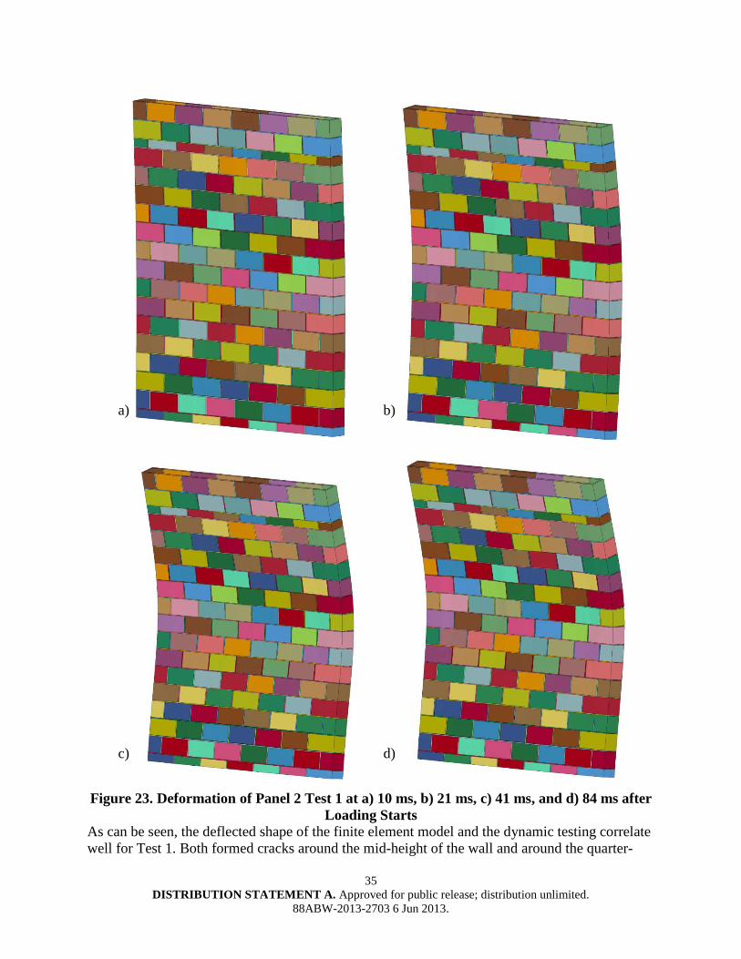
35 DISTRIBUTION STATEMENT A. Approved for public release; distribution unlimited.
88ABW-2013-2703 6 Jun 2013.
a)
c)
b)
d)
Figure 23. Deformation of Panel 2 Test 1 at a) 10 ms, b) 21 ms, c) 41 ms, and d) 84 ms after
Loading Starts As can be seen, the deflected shape of the finite element model and the dynamic testing correlate well for Test 1. Both formed cracks around the mid-height of the wall and around the quarter-
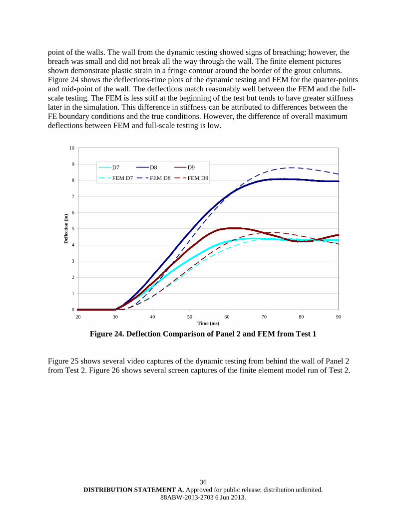
36 DISTRIBUTION STATEMENT A. Approved for public release; distribution unlimited.
88ABW-2013-2703 6 Jun 2013.
point of the walls. The wall from the dynamic testing showed signs of breaching; however, the breach was small and did not break all the way through the wall. The finite element pictures shown demonstrate plastic strain in a fringe contour around the border of the grout columns. Figure 24 shows the deflections-time plots of the dynamic testing and FEM for the quarter-points and mid-point of the wall. The deflections match reasonably well between the FEM and the full-scale testing. The FEM is less stiff at the beginning of the test but tends to have greater stiffness later in the simulation. This difference in stiffness can be attributed to differences between the FE boundary conditions and the true conditions. However, the difference of overall maximum deflections between FEM and full-scale testing is low.
0
1
2
3
4
5
6
7
8
9
10
20 30 40 50 60 70 80 90Time (ms)
Def
lect
ion
(in)
D7 D8 D9
FEM D7 FEM D8 FEM D9
Figure 24. Deflection Comparison of Panel 2 and FEM from Test 1
Figure 25 shows several video captures of the dynamic testing from behind the wall of Panel 2 from Test 2. Figure 26 shows several screen captures of the finite element model run of Test 2.
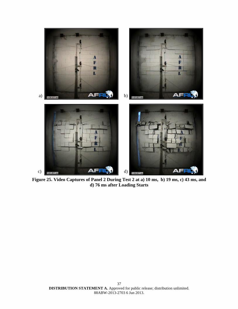
37 DISTRIBUTION STATEMENT A. Approved for public release; distribution unlimited.
88ABW-2013-2703 6 Jun 2013.
a)
c)
b)
d)
Figure 25. Video Captures of Panel 2 During Test 2 at a) 10 ms, b) 19 ms, c) 43 ms, and d) 76 ms after Loading Starts
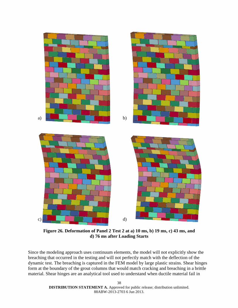
38 DISTRIBUTION STATEMENT A. Approved for public release; distribution unlimited.
88ABW-2013-2703 6 Jun 2013.
a)
c)
b)
d)
Figure 26. Deformation of Panel 2 Test 2 at a) 10 ms, b) 19 ms, c) 43 ms, and d) 76 ms after Loading Starts
Since the modeling approach uses continuum elements, the model will not explicitly show the breaching that occurred in the testing and will not perfectly match with the deflection of the dynamic test. The breaching is captured in the FEM model by large plastic strains. Shear hinges form at the boundary of the grout columns that would match cracking and breaching in a brittle material. Shear hinges are an analytical tool used to understand when ductile material fail in
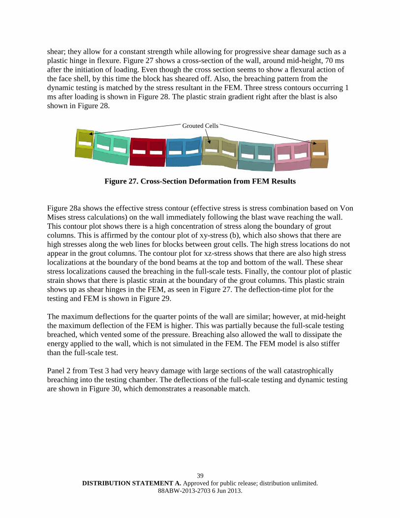
39 DISTRIBUTION STATEMENT A. Approved for public release; distribution unlimited.
88ABW-2013-2703 6 Jun 2013.
shear; they allow for a constant strength while allowing for progressive shear damage such as a plastic hinge in flexure. Figure 27 shows a cross-section of the wall, around mid-height, 70 ms after the initiation of loading. Even though the cross section seems to show a flexural action of the face shell, by this time the block has sheared off. Also, the breaching pattern from the dynamic testing is matched by the stress resultant in the FEM. Three stress contours occurring 1 ms after loading is shown in Figure 28. The plastic strain gradient right after the blast is also shown in Figure 28.
Grouted Cells
Figure 27. Cross-Section Deformation from FEM Results
Figure 28a shows the effective stress contour (effective stress is stress combination based on Von Mises stress calculations) on the wall immediately following the blast wave reaching the wall. This contour plot shows there is a high concentration of stress along the boundary of grout columns. This is affirmed by the contour plot of xy-stress (b), which also shows that there are high stresses along the web lines for blocks between grout cells. The high stress locations do not appear in the grout columns. The contour plot for xz-stress shows that there are also high stress localizations at the boundary of the bond beams at the top and bottom of the wall. These shear stress localizations caused the breaching in the full-scale tests. Finally, the contour plot of plastic strain shows that there is plastic strain at the boundary of the grout columns. This plastic strain shows up as shear hinges in the FEM, as seen in Figure 27. The deflection-time plot for the testing and FEM is shown in Figure 29. The maximum deflections for the quarter points of the wall are similar; however, at mid-height the maximum deflection of the FEM is higher. This was partially because the full-scale testing breached, which vented some of the pressure. Breaching also allowed the wall to dissipate the energy applied to the wall, which is not simulated in the FEM. The FEM model is also stiffer than the full-scale test. Panel 2 from Test 3 had very heavy damage with large sections of the wall catastrophically breaching into the testing chamber. The deflections of the full-scale testing and dynamic testing are shown in Figure 30, which demonstrates a reasonable match.
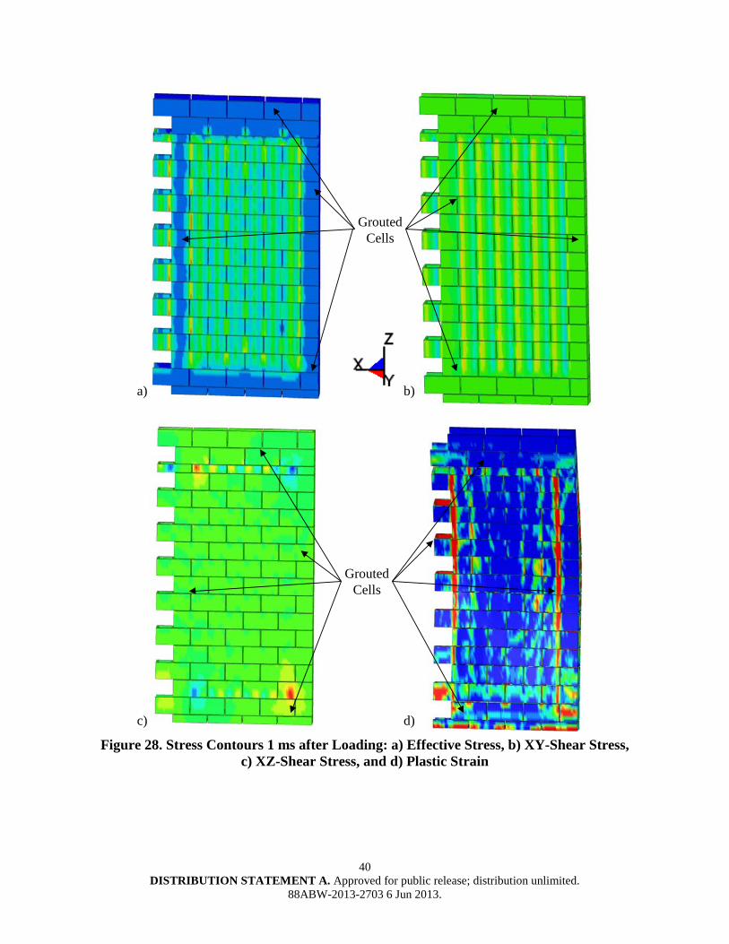
40 DISTRIBUTION STATEMENT A. Approved for public release; distribution unlimited.
88ABW-2013-2703 6 Jun 2013.
Grouted Cells
Grouted Cells
a)
c)
b)
d)
Figure 28. Stress Contours 1 ms after Loading: a) Effective Stress, b) XY-Shear Stress, c) XZ-Shear Stress, and d) Plastic Strain
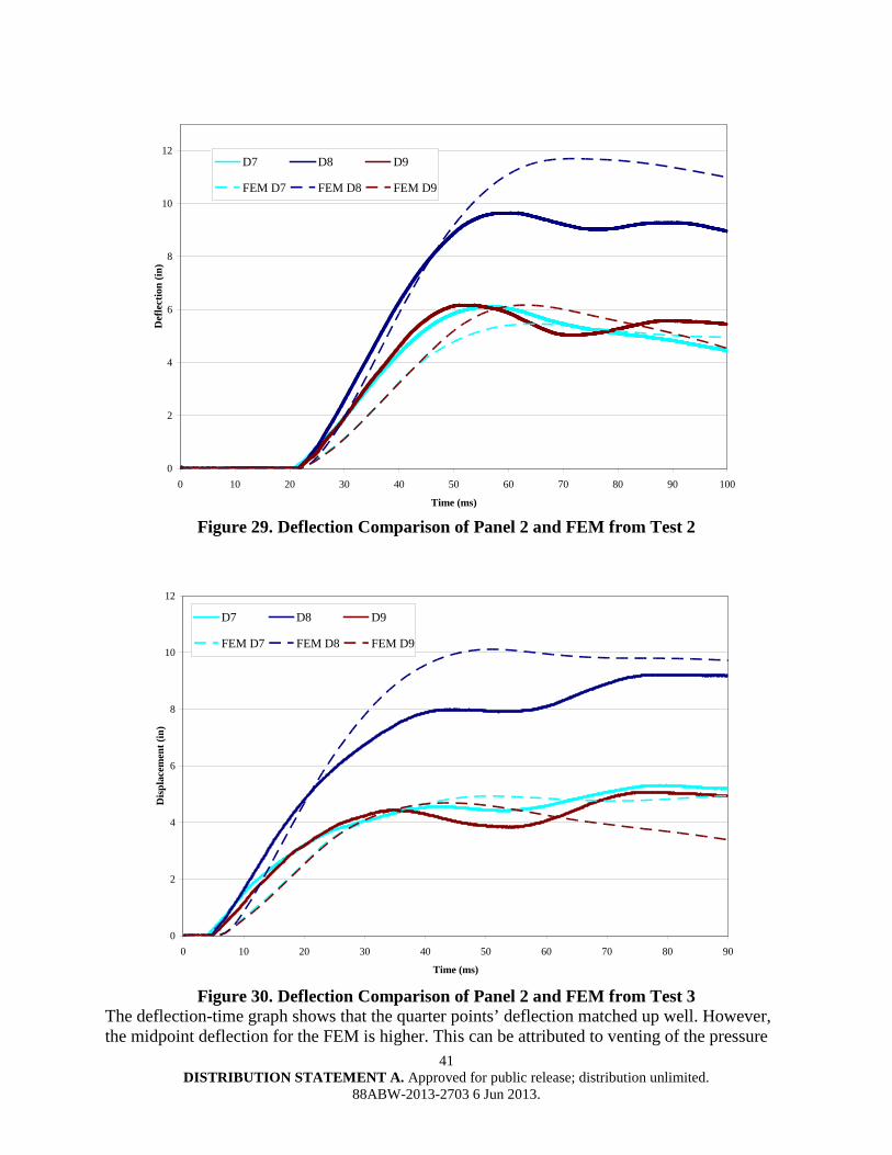
41 DISTRIBUTION STATEMENT A. Approved for public release; distribution unlimited.
88ABW-2013-2703 6 Jun 2013.
0
2
4
6
8
10
12
0 10 20 30 40 50 60 70 80 90 100
Time (ms)
Def
lect
ion
(in)
D7 D8 D9
FEM D7 FEM D8 FEM D9
Figure 29. Deflection Comparison of Panel 2 and FEM from Test 2
0
2
4
6
8
10
12
0 10 20 30 40 50 60 70 80 90
Time (ms)
Dis
plac
emen
t (in
)
D7 D8 D9
FEM D7 FEM D8 FEM D9
Figure 30. Deflection Comparison of Panel 2 and FEM from Test 3
The deflection-time graph shows that the quarter points’ deflection matched up well. However, the midpoint deflection for the FEM is higher. This can be attributed to venting of the pressure
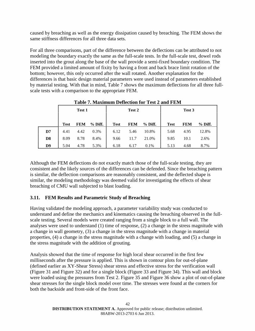
42 DISTRIBUTION STATEMENT A. Approved for public release; distribution unlimited.
88ABW-2013-2703 6 Jun 2013.
caused by breaching as well as the energy dissipation caused by breaching. The FEM shows the same stiffness differences for all three data sets. For all three comparisons, part of the difference between the deflections can be attributed to not modeling the boundary exactly the same as the full-scale tests. In the full-scale test, dowel rods inserted into the grout along the base of the wall provide a semi-fixed boundary condition. The FEM provided a limited amount of fixity by having a front and back brace limit rotation of the bottom; however, this only occurred after the wall rotated. Another explanation for the differences is that basic design material parameters were used instead of parameters established by material testing. With that in mind, Table 7 shows the maximum deflections for all three full-scale tests with a comparison to the appropriate FEM.
Table 7. Maximum Deflection for Test 2 and FEM Test 1 Test 2 Test 3
Test FEM % Diff. Test FEM % Diff. Test FEM % Diff.
D7 4.41 4.42 0.3% 6.12 5.46 10.8% 5.68 4.95 12.8%
D8 8.09 8.78 8.4% 9.66 11.7 21.0% 9.85 10.1 2.6%
D9 5.04 4.78 5.3% 6.18 6.17 0.1% 5.13 4.68 8.7% Although the FEM deflections do not exactly match those of the full-scale testing, they are consistent and the likely sources of the differences can be defended. Since the breaching pattern is similar, the deflection comparisons are reasonably consistent, and the deflected shape is similar, the modeling methodology was deemed valid for investigating the effects of shear breaching of CMU wall subjected to blast loading. 3.11. FEM Results and Parametric Study of Breaching
Having validated the modeling approach, a parameter variability study was conducted to understand and define the mechanics and kinematics causing the breaching observed in the full-scale testing. Several models were created ranging from a single block to a full wall. The analyses were used to understand (1) time of response, (2) a change in the stress magnitude with a change in wall geometry, (3) a change in the stress magnitude with a change in material properties, (4) a change in the stress magnitude with a change with loading, and (5) a change in the stress magnitude with the addition of grouting. Analysis showed that the time of response for high local shear occurred in the first few milliseconds after the pressure is applied. This is shown in contour plots for out-of-plane (defined earlier as XY-Shear Stress) shear stress and effective stress for the verification wall (Figure 31 and Figure 32) and for a single block (Figure 33 and Figure 34). This wall and block were loaded using the pressures from Test 2. Figure 35 and Figure 36 show a plot of out-of-plane shear stresses for the single block model over time. The stresses were found at the corners for both the backside and front-side of the front face.
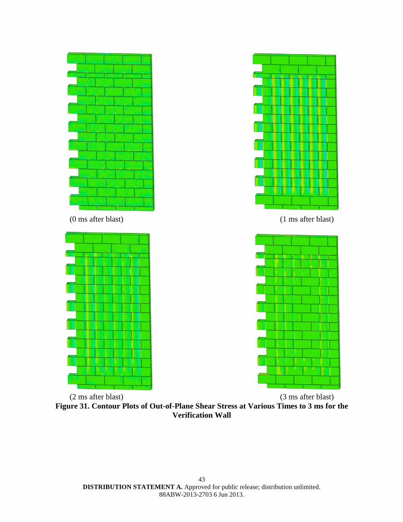
43 DISTRIBUTION STATEMENT A. Approved for public release; distribution unlimited.
88ABW-2013-2703 6 Jun 2013.
(0 ms after blast) (1 ms after blast)
(2 ms after blast) (3 ms after blast)
Figure 31. Contour Plots of Out-of-Plane Shear Stress at Various Times to 3 ms for the Verification Wall
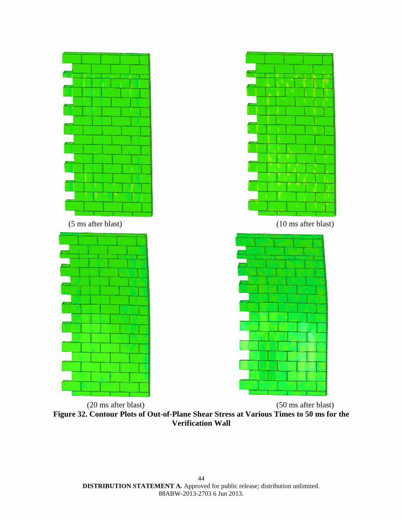
44 DISTRIBUTION STATEMENT A. Approved for public release; distribution unlimited.
88ABW-2013-2703 6 Jun 2013.
(5 ms after blast) (10 ms after blast)
(20 ms after blast) (50 ms after blast)
Figure 32. Contour Plots of Out-of-Plane Shear Stress at Various Times to 50 ms for the Verification Wall
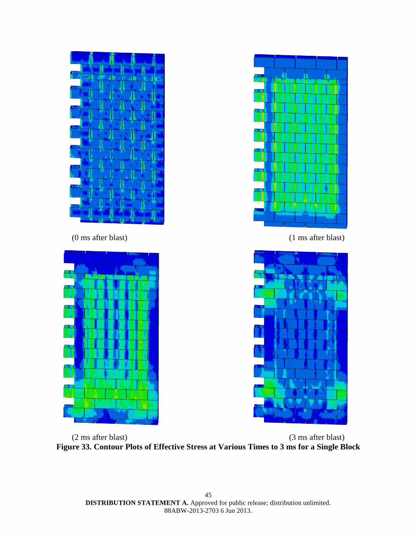
45 DISTRIBUTION STATEMENT A. Approved for public release; distribution unlimited.
88ABW-2013-2703 6 Jun 2013.
(0 ms after blast) (1 ms after blast)
(2 ms after blast) (3 ms after blast)
Figure 33. Contour Plots of Effective Stress at Various Times to 3 ms for a Single Block
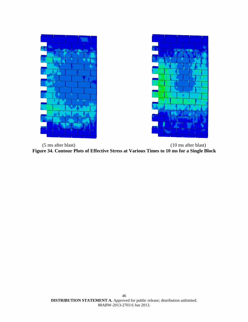
46 DISTRIBUTION STATEMENT A. Approved for public release; distribution unlimited.
88ABW-2013-2703 6 Jun 2013.
(5 ms after blast) (10 ms after blast)
Figure 34. Contour Plots of Effective Stress at Various Times to 10 ms for a Single Block
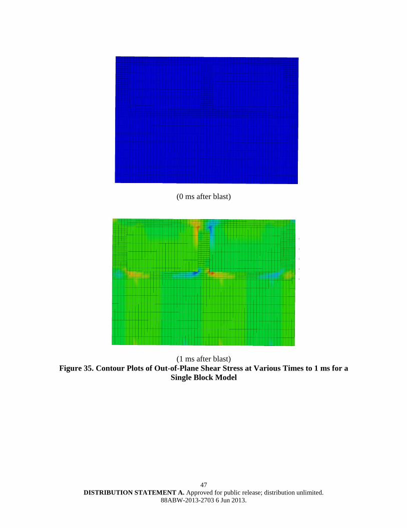
47 DISTRIBUTION STATEMENT A. Approved for public release; distribution unlimited.
88ABW-2013-2703 6 Jun 2013.
(0 ms after blast)
(1 ms after blast)
Figure 35. Contour Plots of Out-of-Plane Shear Stress at Various Times to 1 ms for a Single Block Model
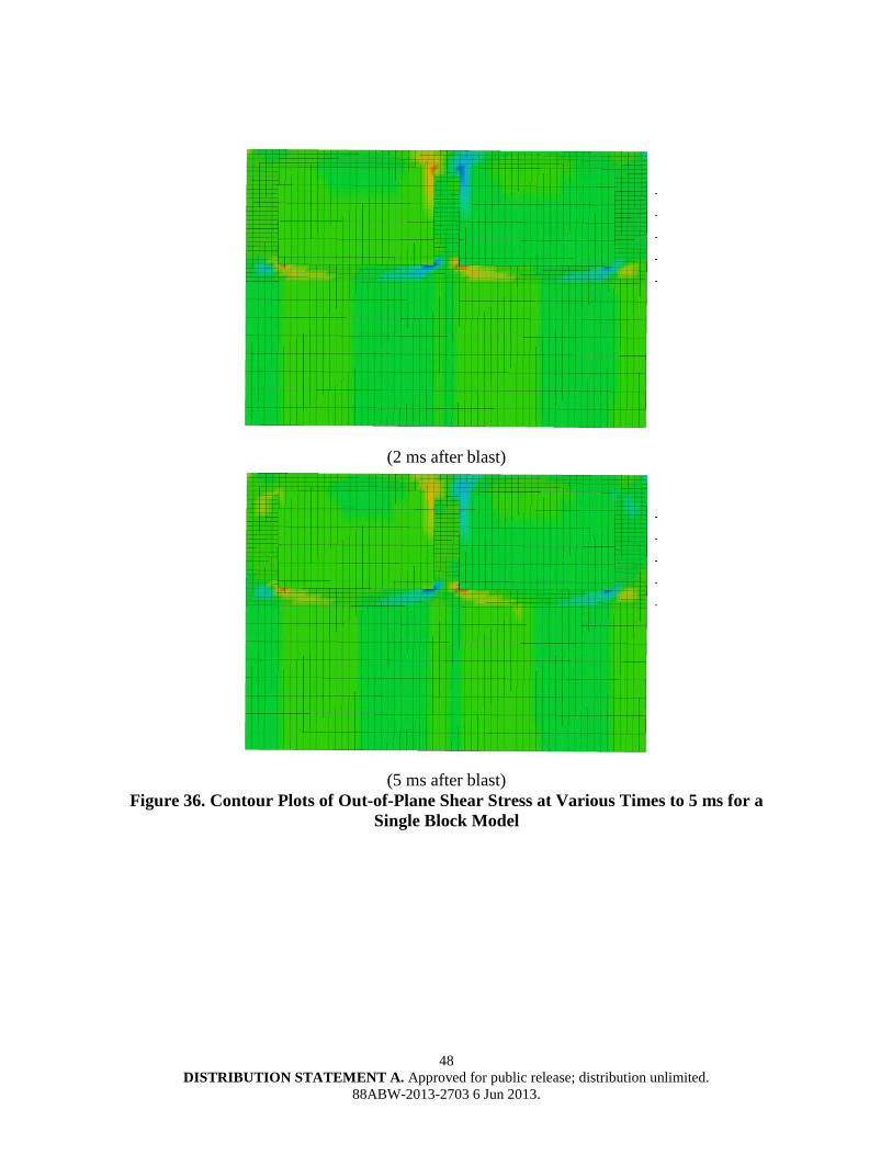
48 DISTRIBUTION STATEMENT A. Approved for public release; distribution unlimited.
88ABW-2013-2703 6 Jun 2013.
(2 ms after blast)
(5 ms after blast)
Figure 36. Contour Plots of Out-of-Plane Shear Stress at Various Times to 5 ms for a Single Block Model

49 DISTRIBUTION STATEMENT A. Approved for public release; distribution unlimited.
88ABW-2013-2703 6 Jun 2013.
(1 ms after blast)
(2 ms after blast)
Figure 37. Contour Plots of Effective Stress at Various Times to 2 ms
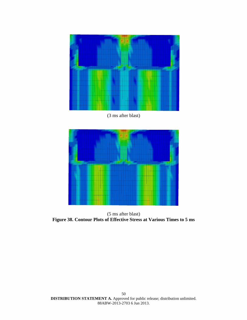
50 DISTRIBUTION STATEMENT A. Approved for public release; distribution unlimited.
88ABW-2013-2703 6 Jun 2013.
(3 ms after blast)
(5 ms after blast)
Figure 38. Contour Plots of Effective Stress at Various Times to 5 ms
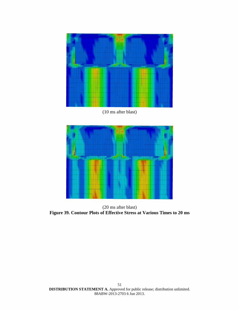
51 DISTRIBUTION STATEMENT A. Approved for public release; distribution unlimited.
88ABW-2013-2703 6 Jun 2013.
(10 ms after blast)
(20 ms after blast)
Figure 39. Contour Plots of Effective Stress at Various Times to 20 ms
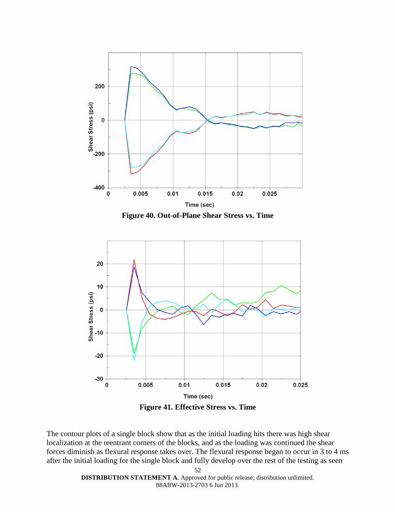
52 DISTRIBUTION STATEMENT A. Approved for public release; distribution unlimited.
88ABW-2013-2703 6 Jun 2013.
Figure 40. Out-of-Plane Shear Stress vs. Time
Figure 41. Effective Stress vs. Time
The contour plots of a single block show that as the initial loading hits there was high shear localization at the reentrant corners of the blocks, and as the loading was continued the shear forces diminish as flexural response takes over. The flexural response began to occur in 3 to 4 ms after the initial loading for the single block and fully develop over the rest of the testing as seen
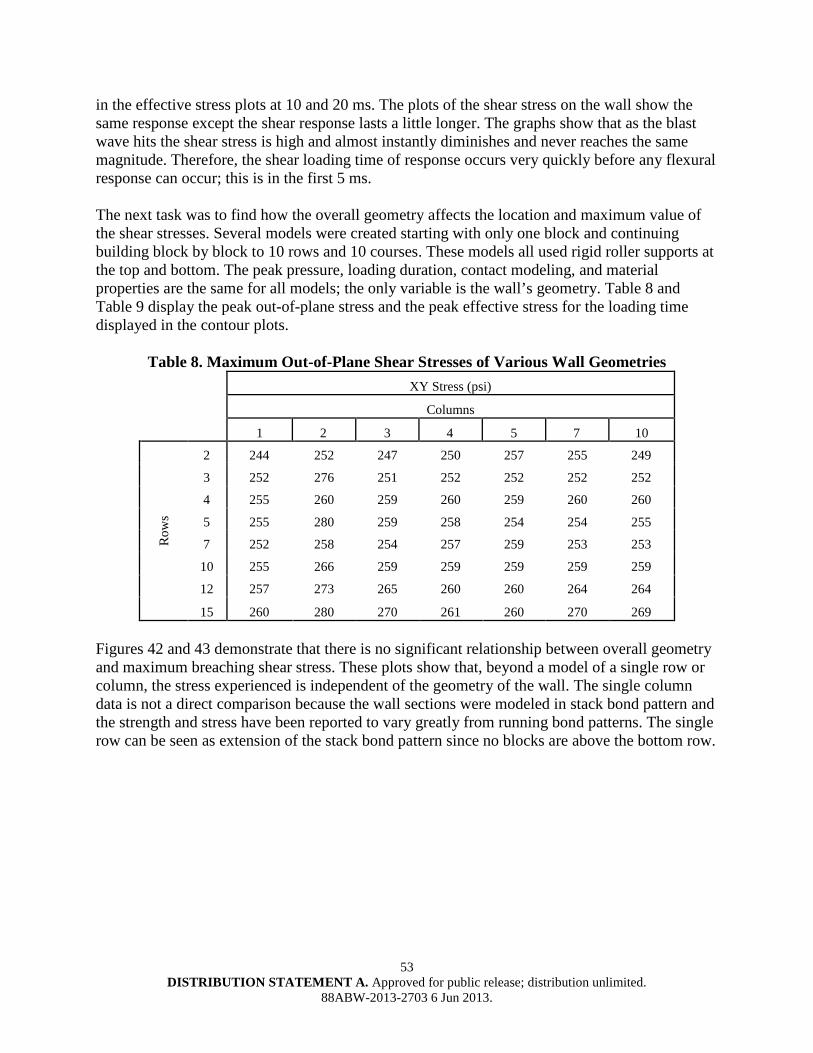
53 DISTRIBUTION STATEMENT A. Approved for public release; distribution unlimited.
88ABW-2013-2703 6 Jun 2013.
in the effective stress plots at 10 and 20 ms. The plots of the shear stress on the wall show the same response except the shear response lasts a little longer. The graphs show that as the blast wave hits the shear stress is high and almost instantly diminishes and never reaches the same magnitude. Therefore, the shear loading time of response occurs very quickly before any flexural response can occur; this is in the first 5 ms. The next task was to find how the overall geometry affects the location and maximum value of the shear stresses. Several models were created starting with only one block and continuing building block by block to 10 rows and 10 courses. These models all used rigid roller supports at the top and bottom. The peak pressure, loading duration, contact modeling, and material properties are the same for all models; the only variable is the wall’s geometry. Table 8 and Table 9 display the peak out-of-plane stress and the peak effective stress for the loading time displayed in the contour plots.
Table 8. Maximum Out-of-Plane Shear Stresses of Various Wall Geometries
XY Stress (psi)
Columns
1 2 3 4 5 7 10
Row
s
2 244 252 247 250 257 255 249
3 252 276 251 252 252 252 252
4 255 260 259 260 259 260 260
5 255 280 259 258 254 254 255
7 252 258 254 257 259 253 253
10 255 266 259 259 259 259 259
12 257 273 265 260 260 264 264
15 260 280 270 261 260 270 269 Figures 42 and 43 demonstrate that there is no significant relationship between overall geometry and maximum breaching shear stress. These plots show that, beyond a model of a single row or column, the stress experienced is independent of the geometry of the wall. The single column data is not a direct comparison because the wall sections were modeled in stack bond pattern and the strength and stress have been reported to vary greatly from running bond patterns. The single row can be seen as extension of the stack bond pattern since no blocks are above the bottom row.
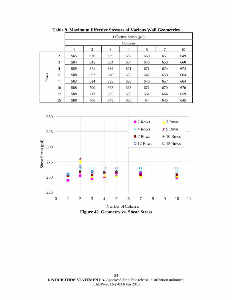
54 DISTRIBUTION STATEMENT A. Approved for public release; distribution unlimited.
88ABW-2013-2703 6 Jun 2013.
Table 9. Maximum Effective Stresses of Various Wall Geometries
Effective Stress (psi)
Columns
1 2 3 4 5 7 10 R
ows
2 565 676 639 652 660 651 649
3 584 645 634 634 646 653 660
4 589 671 666 671 671 674 674
5 588 662 640 638 647 658 664
7 583 614 635 636 646 657 664
10 588 700 668 668 671 670 670
12 588 713 669 659 661 664 659
15 588 706 645 636 64 645 645
225
250
275
300
325
350
0 1 2 3 4 5 6 7 8 9 10 11
Number of Columns
Shea
r Stre
ss (p
si)
2 Rows 3 Rows
4 Rows 5 Rows
7 Rows 10 Rows
12 Rows 15 Rows
Figure 42. Geometry vs. Shear Stress
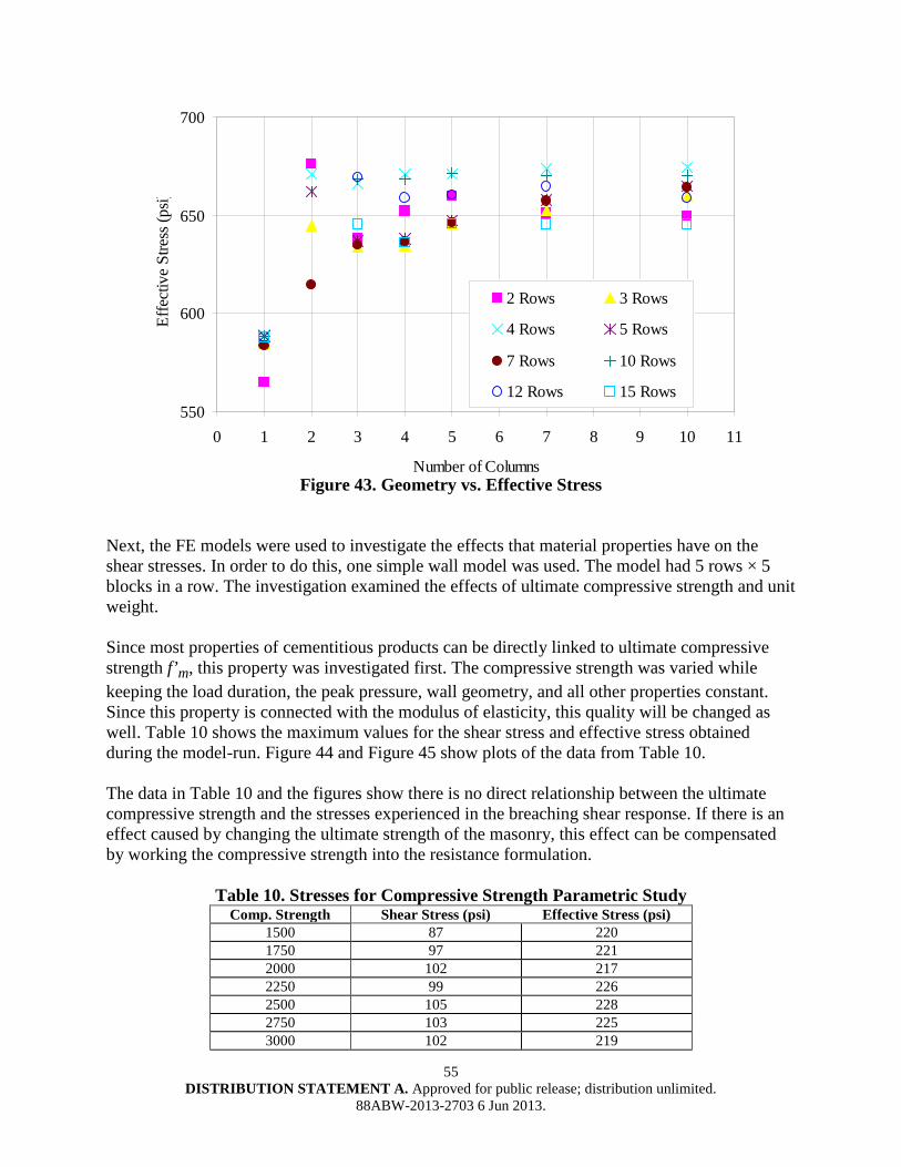
55 DISTRIBUTION STATEMENT A. Approved for public release; distribution unlimited.
88ABW-2013-2703 6 Jun 2013.
550
600
650
700
0 1 2 3 4 5 6 7 8 9 10 11
Number of Columns
Effe
ctiv
e St
ress
(psi)
2 Rows 3 Rows
4 Rows 5 Rows
7 Rows 10 Rows
12 Rows 15 Rows
Figure 43. Geometry vs. Effective Stress
Next, the FE models were used to investigate the effects that material properties have on the shear stresses. In order to do this, one simple wall model was used. The model had 5 rows × 5 blocks in a row. The investigation examined the effects of ultimate compressive strength and unit weight. Since most properties of cementitious products can be directly linked to ultimate compressive strength f’m, this property was investigated first. The compressive strength was varied while keeping the load duration, the peak pressure, wall geometry, and all other properties constant. Since this property is connected with the modulus of elasticity, this quality will be changed as well. Table 10 shows the maximum values for the shear stress and effective stress obtained during the model-run. Figure 44 and Figure 45 show plots of the data from Table 10. The data in Table 10 and the figures show there is no direct relationship between the ultimate compressive strength and the stresses experienced in the breaching shear response. If there is an effect caused by changing the ultimate strength of the masonry, this effect can be compensated by working the compressive strength into the resistance formulation.
Table 10. Stresses for Compressive Strength Parametric Study Comp. Strength Shear Stress (psi) Effective Stress (psi)
1500 87 220 1750 97 221 2000 102 217 2250 99 226 2500 105 228 2750 103 225 3000 102 219
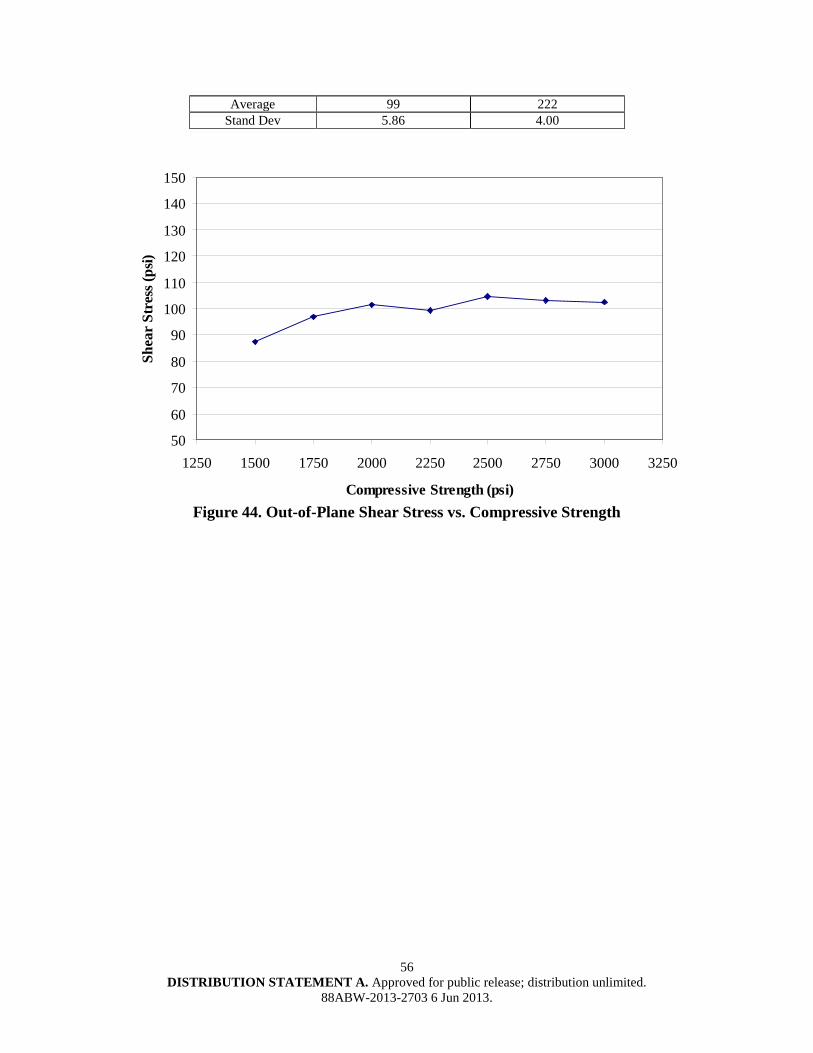
56 DISTRIBUTION STATEMENT A. Approved for public release; distribution unlimited.
88ABW-2013-2703 6 Jun 2013.
Average 99 222 Stand Dev 5.86 4.00
50
60
70
80
90
100
110
120
130
140
150
1250 1500 1750 2000 2250 2500 2750 3000 3250
Compressive Strength (psi)
Shea
r St
ress
(psi)
Figure 44. Out-of-Plane Shear Stress vs. Compressive Strength
57 DISTRIBUTION STATEMENT A. Approved for public release; distribution unlimited.
88ABW-2013-2703 6 Jun 2013.
200
210
220
230
240
250
1250 1500 1750 2000 2250 2500 2750 3000 3250
Compressive Strength (psi)
Effe
ctiv
e St
ress
(psi)
Figure 45. Effective Stress vs. Compressive Strength
The next parameter was the unit weight of the CMU. Since the loading is dynamic, a change in the overall mass or weight of the system should cause a change in the stress of the response. In order to do this, the same wall as used for the compressive strength parametric study was used and the unit weight was changed from light weight concrete to middle weight concrete. Even though the modulus of elasticity is connected with the unit weight, the modulus of elasticity remained constant for these analyses. Table 11 shows the maximum values for the shear stress and effective stress of the parametric study over the run-time of the model. Figure 46 and Figure 47 show plots of the data in Table 11. The effective stress plot demonstrates a downward trend of stress as the unit weight goes up. This is to be expected as an increase in unit weight gives an increase in mass of the system. However, the decrease is relatively minor over the range of unit weights. The other figures show that there is a uniform stress value for the same loading for all unit weights and that there is no direct relationship between breaching shear stress and unit weight.
58 DISTRIBUTION STATEMENT A. Approved for public release; distribution unlimited.
88ABW-2013-2703 6 Jun 2013.
Table 11. Stresses for Compressive Strength Parametric Study Unit Weight
(lb/ft3) Shear Stress (psi) Effective Stress (psi)
85 103 221 90 100 222 95 102 222
100 99.1 221 105 100 220 110 100 220 115 101 219 120 103 218 125 102 217 130 104 217 135 104 216 140 102 216 145 100 216
150 100 216
80
90
100
110
120
130
140
150
80 90 100 110 120 130 140 150
Unit Weight (lb/ft3)
Shea
r St
ress
(psi)
Figure 46. Out-of-Plane Shear Stress vs. Unit Weight
59 DISTRIBUTION STATEMENT A. Approved for public release; distribution unlimited.
88ABW-2013-2703 6 Jun 2013.
200
210
220
230
240
250
80 90 100 110 120 130 140 150
Unit Weight (lb/ft3)
Effe
ctiv
e St
ress
(psi)
Figure 47. Effective Stress vs. Unit Weight
Next, the effects of loading were investigated. The first investigation into loading was whether a change in impulse affected the magnitude of the shear stress. The loading shapes were the simplified triangular pulse load and rectangular load. The maximum loading pressure and loading duration were held constant, and only the shape was changed; therefore, the applied impulse for the rectangular loading was twice the impulse as the triangular loading. These loading shapes are seen in Figure 48. Various FEMs, from geometry testing, were modified in order to analyze the loading shape’s influence on the breaching phenomenon. Table 12 shows the out-of-plane shear stress and effective stress for the triangular and rectangular pulse shapes. Table 13 shows that there is a difference between the rectangular and triangular load in all stresses. The shear stress difference is as high as 40.8 psi. However, for the most part, the difference in shear stress is less than 30 psi. There is an average percent difference of less than 10% and a standard deviation of less than 10 psi. Therefore, the data shows that the shear stress is not greatly affected by increasing the impulse, such as doubling the impulse.
60 DISTRIBUTION STATEMENT A. Approved for public release; distribution unlimited.
88ABW-2013-2703 6 Jun 2013.
Figure 48. Normalized Loading Distribution
Table 12. Stresses from Loading Shape Parametric Study Wall
Geometry Shear Stress (psi) Effective Stress (psi)
Tri. Rect. Tri. Rect. 3x3 267 290 646 695 3x5 284 307 668 715 3x7 267 290 647 694
3x10 252 290 660 694 5x3 265 288 646 693 5x5 282 306 671 718 5x7 265 306 646 718
5x10 282 306 671 719 10x3 265 288 657 713 10x5 265 288 659 717 10x7 265 288 665 715 10x10 265 288 659 716
Po
Td Normalized Time
Nor
mal
ized
Pre
ssur
e
61 DISTRIBUTION STATEMENT A. Approved for public release; distribution unlimited.
88ABW-2013-2703 6 Jun 2013.
Table 13. Statistical Data from the Loading Shape Parametric Study
Wall Geometry
Shear Stress (psi) Effective Stress (psi)
Difference % Diff. Difference % Diff. 3x3 23 8.5% 49 7.6% 3x5 22 7.8% 47 7.1%
3x7 23 8.6% 47 7.3%
3x10 38 15% 34 5.2% 5x3 23 8.7% 48 7.4% 5x5 23 8.3% 48 7.1% 5x7 41 15.4% 72 11%
5x10 24 8.4% 47 7.1% 10x3 23 8.8% 56 8.6% 10x5 23 8.7% 58 8.8% 10x7 23 8.7% 51 7.6% 10x10 23 8.7% 58 8.7%
Aver. 26 9.7% 51 7.8%
The differences in peak pressure were examined to see if it caused any difference in magnitude of the shear stresses. Only three FEM’s were used, and only the peak pressure in both triangular and rectangular loading shape was varied. Table 14–Table 16 show the data from the peak pressure parametric study for three different walls. Figure 49 and Figure 50 show plots of the data from Table 14–Table 16. The data show that there is a relationship between peak pressure and breaching stress values. The relationship is approximately linear. The R-squared values are all above 0.95 indicating a good fit for linear regression. Therefore, there is approximately a linear relationship between applied pressure and stress values.
Table 14. Stresses from the 5 × 5 Wall from the Peak Pressure Parametric Study Peak
Pressure (psi)
Triangular Rectangular Shear
Stress (psi) Effect.
Stress (psi) Shear
Stress (psi) Effect.
Stress (psi) 5 54 133 61 152
10 102 217 112 244 15 122 321 135 344 20 140 359 151 384 25 149 374 162 411 30 163 421 178 458 35 190 485 208 520 40 223 546 243 589 45 254 616 273 658 50 282 671 306 718
62 DISTRIBUTION STATEMENT A. Approved for public release; distribution unlimited.
88ABW-2013-2703 6 Jun 2013.
Table 15. Stresses from the 10 × 3 Wall from the Peak Pressure Parametric Study Peak
Pressure (psi)
Triangular Rectangular Shear Stress
(psi) Effect. Stress
(psi) Shear Stress
(psi) Effect. Stress
(psi) 5 54.1 135.9 60.4 155
10 86.9 214 98.0 244 15 120 302.4 135 330 20 138 334.5 149 363 25 151 373.4 166 423 30 169 426.8 187 475 35 187 487.8 208 537 40 215 558.8 237 611 45 238 611.8 259 658 50 265 658.7 288 713
Table 16. Stresses from the 3 × 10 Wall of the Peak Pressure Parametric Study Peak
Pressure (psi)
Triangular Rectangular Shear
Stress (psi) Effect.
Stress (psi) Shear
Stress (psi) Effect.
Stress (psi) 5 54.2 134 54.2 134
10 94.7 209 94.7 209 15 122 320 122 320 20 137 370 137 370 25 159 388 159 388 30 196 407 196 407 35 201 477 201 477 40 218 536 218 536 45 240 599 240 599 50 252 660 290 694
63 DISTRIBUTION STATEMENT A. Approved for public release; distribution unlimited.
88ABW-2013-2703 6 Jun 2013.
0
50
100
150
200
250
300
0 10 20 30 40 50 60Load (psi)
Shea
r St
ress
(psi
)
T 5x5 T 10x3 T 3x10
Figure 49. Out-of-Plane Shear Stress vs. Peak Pressure
0
200
400
600
800
1000
1200
0 10 20 30 40 50 60Peak Pressure (psi)
Effe
ctiv
e St
ress
(psi
)
T 5x5 T 10x3 T 3x10
Figure 50. Effective Stress vs. Peak Pressure
64 DISTRIBUTION STATEMENT A. Approved for public release; distribution unlimited.
88ABW-2013-2703 6 Jun 2013.
The final investigation looks at the effects of grouting. In order to do this, several wall models were created that include grout. All models using grout were partially grouted. Table 17 shows values for the maximum out-of-plane shear stresses for both grouted and non-grouted models occurring immediately after the blast wave hits the wall. Figure 51 and Figure 52 show graphical representations of the data in Table 17. As can be seen from the figures, the grouted sections resulted in higher shear stresses, which can be attributed to the fact that the wall sections around the grouted columns are stiffer and would attract a higher percentage of the internal forces. The models were only grouted in the end cells of the models, so an increase in the number of blocks would increase the distance between grouted cells. There is however no correlation between the distances between grouted columns and the shear stress values. This indicates that for the breaching shear effect, the maximum shear stress is independent of where the grout is placed.
Table 17. Grouted vs. Non-Grouted Maximum Stresses Shear Stress (psi) Effective Stress (psi)
Non-Grouted Grouted Difference Non-
Grouted Grouted Difference
5x3 265 266 0.9 646 780 135 5x5 282 280 2.2 671 870 199 5x7 265 289 24 646 833 187
5x10 282 294 12 671 839 168 7x3 254 280 27 635 799 164 7x5 259 284 25 646 717 71.2 7x7 253 289 36 657 717 59.5
7x10 253 282 29 664 726 62.1 10x3 265 268 3.8 657 897 240 10x5 265 277 13 659 827 168 10x7 265 281 17 665 751 86.6 10x10 265 277 13 659 783 124 12x3 259 266 7.0 669 847 177 12x5 265 276 11 661 823 162 12x7 265 276 12 664 788 124 12x10 265 277 12 659 774 115 15x3 265 267 2.2 645 702 56.8 15x5 265 293 28 636 720 84.5 15x7 265 277 12 645 714 68.2 15x10 265 299 34 645 726 80.5
65 DISTRIBUTION STATEMENT A. Approved for public release; distribution unlimited.
88ABW-2013-2703 6 Jun 2013.
250255
260265
270275
280285
290295
300305
2 4 6 8 10 12Number Blocks along Length
Shea
r St
ress
(psi)
Non-Grouted Grouted
Figure 51. Out-of-Plane Shear Stresses for Grouted and Non-Grouted Walls
600
650
700
750
800
850
900
950
2 4 6 8 10 12Number of Blocks along Length
Effe
ctiv
e St
ress
(psi)
Non-Grouted Grouted
Figure 52. Effective Stresses for Grouted and Non-Grouted Walls

66 DISTRIBUTION STATEMENT A. Approved for public release; distribution unlimited.
88ABW-2013-2703 6 Jun 2013.
4. RESULTS AND DISCUSSIONS
4.1. Introduction
This chapter presents the development of engineering-level design equations for direct shear in CMU walls subjected to blast loading. These design equations must provide an adequate prediction of the resistance of the system without being overly conservative. Since the system is dynamic, an overview of structural dynamics is given with a focus on approximate modeling towards understanding the breaching phenomenon of CMU walls. The properties of the wall are determined, allowing a single block or a group of blocks to be modeled as quasi-static, which allows the wall to be conceptualized as a static beam. Finally, the structural analysis will allow for the development of a nominal shear force according to the maximum pressure and the development of a shear resistance equation. 4.2. Structural Dynamics
In order to better understand the breaching phenomenon, a dynamic analysis of the wall was carried out. Complex multiple DOF systems are too complicated for most practicing design engineers; therefore, the complex system must be idealized as a simplified one-way system whenever possible. The following section gives an overview of SDOF systems plus the added simplifications that can be used for special cases. 4.2.1. SDOF Model A SDOF system involves only one way for the system to move, hence a single degree-of-freedom. This is extended to a multiple DOF system where predominant motion can be described by a single motion variable and all other motions can be described by this motion. This DOF can be a displacement or a rotation. Figure 53 shows free body diagram of a lumped-mass, SDOF system.
Figure 53. SDOF Idealization
The system has four forces acting on it. These forces are inertia-induced force, stiffness-induced force, damping-induced force, and the applied force. Putting the above system in equilibrium produces
m k cF F F F(t)+ + = (9)
67 DISTRIBUTION STATEMENT A. Approved for public release; distribution unlimited.
88ABW-2013-2703 6 Jun 2013.
where Fm = mass-induced force, Fk = stiffness-induced force, Fc = damping-induced force, and F(t) = forcing function or applied force according to time. Using Newton’s law of motion, mass-induced force is equal to mass times the acceleration given by
mF ma my= = (10) where m = mass of the system and a = y = acceleration of the system. The acceleration is defined as the second derivative of the displacement with respect to time. The resistance-induced force is provided by a resistance of the system. This resistance can be conceptualized as a simple spring that has a constant stiffness per unit displacement. This then gives the resistance-induced force as
kF kδ ky= = (11) where k = stiffness of the system per unit displacement and δ = y = displacement. The damping-induced force is provided by friction, cracking, or other energy-absorption mechanism. All the damping effects can be approximated by a viscous damper that requires a constant force to move a body through a viscous liquid at a certain speed. The damping-induced force is given by
cF cv cy= = (12) where c = damping coefficient of the system and v = y = velocity of the system. The velocity is defined as the first derivative of the displacement with respect to time. Substituting Equation 10, 11, and 12 into Equation 9 gives my cy ky F(t)+ + = (13) which is the governing equation for a SDOF system. This equation can be solved to find the solution for a lumped-mass system. With the full dynamic equation known, other properties of the dynamic system can be obtained. In general, the natural frequency ωn of a SDOF system is given by
ω =n
km (14)
68 DISTRIBUTION STATEMENT A. Approved for public release; distribution unlimited.
88ABW-2013-2703 6 Jun 2013.
The natural period of the system Tn is given by
2πω
=nn
T (15)
The natural period is the amount of time that the system takes to complete a full cycle. Unlike in the above lumped-mass idealization, the mass of real structures is distributed over a volume. Equation 13 can still be used, but the analysis becomes difficult for systems with continuous–mass distribution. An approximate method then must be carried out to ease computation. The approximate system is represented by
e e em y k y F (t)+ = (16) where me, ke, and Fe(t) = effective mass, effective resistance, and effective forcing function of the system, respectively. The damping forces are negligible in the blast analyses since damping has a relatively small impact on the peak deflection, so this force is omitted. Equation 14 can be expressed in terms of the real system by
m L LK my K ky K F(t)+ = (17) where Km and KL = mass and load factors, respectively. The damping-induced force is assumed to be zero in the equivalent system. The approximation idealizes that all response will occur in a mode close to the first mode. The idealized system assumes the displacement of the system Φ(x) to be the same as that produced in static loading and the maximum deflection of the system is normalized to unity. This is done to give a better approximation of the effective forces. The equivalent mass, me, resistance, ke, and force, Fe, of a distributed mass system is given by
2deL
m mΦ(x) x= ∫ (18)
eF F(t)Φ(x)= ∫ (19)
e ek F= (20) The mass factor Km and load factors KL are given by
2de L
m
mΦ(x) xmKm m
∫= =
(21)
69 DISTRIBUTION STATEMENT A. Approved for public release; distribution unlimited.
88ABW-2013-2703 6 Jun 2013.
de L
L
FΦ(x) xFKF F
∫= =
(22) Finally, if Equation 14 is divided through by KL, the equation is given by
LmK my ky F(t)+ = (23) where KLm = the load mass factor (ratio of Km to KL). Solution of Equation 23 represents the idealized SDOF response of a system; the displacement can be related to the internal forces and other mechanical characteristics of the system response. The natural frequency of the equivalent system is given by
ω = =e
nee Lm
k km K m (24)
4.2.2. Pressure-Impulse Simplifications A SDOF system can be a convenient simplification for design use. Another approach is to use pressure-impulse (P-I) diagrams to predict the extent to which the member will be damaged under a given loading. A normal response spectrum highlights the influence of structure properties on the response, which can be duration of loading, natural period, natural frequency, or other like properties. P-I diagrams use the load and impulse for a given response. Figure 54a shows the response of an undamped, perfectly elastic SDOF system. Figure 54b shows an equivalent system in a P-I diagram format where Po is the peak pressure, K is the stiffness, M is the mass, xmax is the maximum displacement, I is the impulse, td is the loading duration, and T is the natural frequency. There exist three loading regimes: impulsive, dynamic, and quasi-static. P-I diagrams clearly show all three loading regimes and transfer points between the three regimes. The vertical asymptote is the impulsive regime, the horizontal asymptote is the quasi-static regime, and the line that connects these two is the dynamic regime. These are shown on the response spectrum, but the transfer points are not clearly determined because the curve does not have asymptotic properties in the impulsive regime.
70 DISTRIBUTION STATEMENT A. Approved for public release; distribution unlimited.
88ABW-2013-2703 6 Jun 2013.
a) td/T
xmax
/(Po/K
)
Quasi-Static RegimeImpulsive Regime Dynamic Regime
b) I/(KMxmax)0.5
Po/(
xmax
K)
Quasi-Static Asymtope
Implusive Asymtope
Dynamic Region
Impulsive Asymptote
Quasi-Static Asymptote
I/(KMxmax)0.5
Po/(
xmax
K)
Quasi-Static Asymtope
Implusive Asymtope
Dynamic Region
Impulsive Asymptote
Quasi-Static Asymptote
Figure 54. Response Regimes: a) Response Spectrum and b) P-I Diagram
Some systems can be even further simplified. Figure 55 displays the quasi-static and impulsive regimes emphasizing the duration of loading, td, and time of response, tm.
71 DISTRIBUTION STATEMENT A. Approved for public release; distribution unlimited.
88ABW-2013-2703 6 Jun 2013.
a) Time
Forc
e
tm td
Load FunctionResistance History
b) Figure 55. Loading Regimes: a) Quasi-Static and b) Impulse
Figure 55a is a quasi-static loading case, characterized by the period T being much shorter than the duration of loading td. In quasi-static loading regime, the peak resistance is reached before the loading value has had time to dissipate. Therefore, the resistance of a quasi-static system depends on the peak pressure and not on the loading duration. The regime shown in Figure 55b is an impulsive loading case, characterized by the period of the system being much longer than the duration of loading. In the impulsive loading regime, the load
72 DISTRIBUTION STATEMENT A. Approved for public release; distribution unlimited.
88ABW-2013-2703 6 Jun 2013.
is applied and dissipated before any significant system response has occurred. Therefore, the loading duration has very little impact on the system. A third regime is the dynamic loading regime. The dynamic loading regime is characterized by the loading duration being of the same order as the period of the system. In this regime, the loading duration cannot be uncoupled from the maximum response of the system, and the response is more complex to determine. 4.3. Modeling of Breaching Response
In analyzing the finite element models, there are two structural modeling approaches that could simulate the breaching response. The first is single-block beam analogy; the other is a beam that runs between grout cells. Both models were investigated to determine the best basis for the resistance equation. 4.3.1. Dynamics of the Face Shell Beam Model The finite element analysis showed that there are high shear stresses near the webs of each block for 2 to 3 ms after the pressure reaches the wall. High stresses existed near the webs even when there was grout present in the model. This indicated that each individual block carries only the shear developed on its face with the mortar not facilitating transfer of shear. In addition, the geometry of the wall had no significant influence on the maximum value of shear stress in the non-grouted geometry investigation. Since breaching will not occur at the webs, the beam analogy was modeled with only one cell of the block with the face shell connections to the webs acting as perfectly fixed. Figure 56 shows a single cell of a block represented as a beam and a cross section of the representative beam. Figure 57 illustrates the idealization of the beam as fixed-fixed beam. From this model, the natural period can be obtained.
Figure 56. Face Shell Beam and Cross Section
73 DISTRIBUTION STATEMENT A. Approved for public release; distribution unlimited.
88ABW-2013-2703 6 Jun 2013.
Figure 57. Single Block Beam Representation
The beam has a span length L of one cell, a width h of the full height of the wall, and a thickness t of one face shell. The representative beam has a moment of inertia of
3
12htI =
(25) The mass and the stiffness of the beam are
gγM Lht=
(26)
3384EIk
L=
(27) where γ is the unit weight of the block and g is the acceleration due to gravity. For a fixed-fixed beam under a uniformly distributed load, the assumed displacement equation is
2 2 3 4
416 ( - 2 )Φ(x) L x Lx xL
= + (28)
With this equation, the equivalent mass factor, equivalent load factor, and equivalent load-mass factor are
0.4064MK =
0.5333LK =
0.7619LMK = This gives the equivalent SDOF response equation as
33840.7619 EIMy y F(t)
L+ =
(29)
Po
74 DISTRIBUTION STATEMENT A. Approved for public release; distribution unlimited.
88ABW-2013-2703 6 Jun 2013.
Finally, the natural frequency is given by
3 233 4
384384E g 16,230
0.7619 12 0.7619n
LM
EIk ht EtLω
K M M L γLht γL= = = =
× × (30) Table 18 shows representative numbers of an 8-in CMU. E is Young’s modulus, and f’m is the ultimate compressive strength of the masonry assemblage.
Table 18. Representative Numbers for 8-in CMU f’m 1500 psi
E 1400 ksi
t 1.25 in
γ 125 lb/ft3
L 6.06 in
Substituting the values from Table 18, the natural frequency and natural period are
19000 / s 19 kHznω = =
-43.4 10 s 0.34 msnT = × =
Table 19 gives the following ranges for loading regimes from Blast Effects on Buildings (Smith and Cormie, 2009) and from Modern Protective Structures (Krauthammer, 2008).
Table 19. Loading Regime Ranges Regime Cormie Krauthammer
Impulsive td/Tn < 0.1 td/Tn < 0.0637
Dynamic 0.1 < td/Tn < 10 0.637 < td/Tn < 6.37
Quasi-Static td/Tn > 10 td/Tn > 6.37
The loading duration td is assumed to be 0.01 s or 10 ms at its shortest duration (the shortest duration of the dynamic testing discussed in Section 3 was approximately 14 ms). The natural period gives loading duration to natural period ratio of approximately 30, which corresponds to the quasi-static regimes from both sources. The quasi-static loading can be assumed for loading duration of 3.4 ms or more. Therefore, the breaching of the walls can be assumed to behave as if quasi-static loading is applied and can be modeled by applying a static pressure over the whole wall. This matches well with the FEM results found in the parametric study presented in Section 3, as the shape of the loading did not influence the shear stress but the peak pressure did.
75 DISTRIBUTION STATEMENT A. Approved for public release; distribution unlimited.
88ABW-2013-2703 6 Jun 2013.
4.3.2. Dynamics of Between Grout Cells Beam The finite element analyses demonstrated high shear stresses at the interface between grouted and non-grouted cells in the models with grout present, which indicates that there could be a beam analog that runs between grout cells with the columns idealized as fixed supports. Figure 58 shows the representative beam and cross section of the between grout cell beam (BGC beam). The same approach as used for the single block beam was used with the exception that the beam had a length L of the distance between grout cells, a thickness t of one face shell, width w of the block, and a height h of the height of one block. This model used only the face shells because the breaching will occur in the face shell, not at the web. In addition, the webs have sufficient stiffness to ensure that the face shells have composite action.
Figure 58. BGC Beam and Cross Section A-A
The moment of inertia contributing to stiffness of the section was only the two face shells of the sections assuming composite action; it is represented by
3 22(1/12 ( / 2 / 2) )I ht th w t= + − (31)
76 DISTRIBUTION STATEMENT A. Approved for public release; distribution unlimited.
88ABW-2013-2703 6 Jun 2013.
All other properties are the same for BGC breaching; the effects of reinforcing in the grout cells were assumed to be negligible because the shearing happens between columns. Then, the natural frequency is
2 23n 4
384389,500 (1/12 / 4)
0.7619
EIE t wL
M γLω +
= = (32)
These values are given for CMU ranging from 6-in to 16-in in Table 20 with corresponding natural frequencies, and natural periods. In addition, the table shows the minimum loading duration in which quasi-static analysis can be used. The length is based on maximum bar spacing of 6 times the block’s width subtracting the grouted parts of the length.
Table 20. Quasi-Static Details for between Grouted Cells Beam Size of CMU
w (in)
L (in)
ωn
(103/s) Tn
(ms) Td,min (ms)
6-in 5.625 27.69 11.5 0.547 5.47 8-in 7.625 39.69 83.2 0.832 8.32
10-in 9.625 51.69 5.62 1.12 11.2 12-in 11.625 63.69 4.47 1.41 14.1 14-in 13.625 75.69 3.71 1.70 17.0 16-in 15.625 87.69 3.17 1.99 19.9
Since the blasts considered in this study are at least 15 ms long, 6-in to 12-in CMU can be analyzed using quasi-static for almost all cases. When wider blocks are being used, the loading duration must be found and checked against values determined for natural period. Figure 59–Figure 63 show the effect that different parameters can have on the minimum load duration. The data was generated using inputs for an 8-in CMU block with a unit weight of 125 lb/ft3 only varying the parameter of interest. These graphs cannot be used to determine the minimum load duration; they are only used to show the general effects the parameters have on the minimum load duration.
77 DISTRIBUTION STATEMENT A. Approved for public release; distribution unlimited.
88ABW-2013-2703 6 Jun 2013.
Figure 59. Qualitative Effects: Minimum Load Duration vs. Modulus of Elasticity
Figure 60. Qualitative Effects: Minimum Load Duration vs. Thickness of Face Shell
78 DISTRIBUTION STATEMENT A. Approved for public release; distribution unlimited.
88ABW-2013-2703 6 Jun 2013.
Figure 61. Qualitative Effects: Minimum Load Duration vs. Width of Block
Figure 62. Qualitative Effects: Minimum Load Duration vs. Unit Weight
79 DISTRIBUTION STATEMENT A. Approved for public release; distribution unlimited.
88ABW-2013-2703 6 Jun 2013.
0
10
20
30
40
50
60
70
25 35 45 55 65 75 85 95
Lenght between Shear Surfaces (in)
Loa
d D
urat
ion
Figure 63. Minimum Load Duration vs. Length between Grout Cells
The figures above show that the minimum load duration will change less than 5 ms for the variable ranges considered. This is especially true for the thickness of the face shells, t, which caused less than a 1 ms difference over its range of values. For modulus of elasticity, E, and the unit weight, γ, the variation was small as well. The width did change more rapidly with a variation of 10 ms over the data; however, the width of block would change along with the distance between grouted columns giving a lower variation. This leaves only the distance between shear planes as a major variable; the graph shows that the minimum duration load changes rapidly with length. Therefore, if a load duration is too small to assume quasi-static response for a given wall geometry, the length between grouted columns could be reduced until the quasi-static analysis can be used. 4.3.3. Direct Shear Modeling Since both beam approximations are quasi-static, the complex wall can be analyzed as a one-way beam with fixed supports at both ends. Because of similarities between the models, the beams can be modeled the same with slight variations. The loading area of the beams AL are given by
LA hL= (33) where h = the full height of a single block and L = the length of the member. The total force of the pressure loading FP is given by
PF PhL= (34)
80 DISTRIBUTION STATEMENT A. Approved for public release; distribution unlimited.
88ABW-2013-2703 6 Jun 2013.
where P = the peak pressure resulting from the blast loading. When the pressure is applied to the loading area, the shear force at the supports Vu become
2 2L
uPAPhLV = =
(35) The reaction can quickly be determined to be the shear forces acting at the supports. Therefore, the shear force on the each beam model depends on the height of the wall, the length of the wall, and the peak pressure on the wall. 4.4. Resistance Equation Derivation
The next step is to develop each beam’s nominal resistance. These resistance equations will be based on mechanics and design standards. 4.4.1. Development of Resistance Equation There are three components of shear resistance: strength attributed to masonry, the strength attributed to gravity loading, and the strength attributed to steel. Therefore, the nominal shear Vn resistance is given by
n m p sV V V V= + + (36)
where Vm = the shear resistance of the masonry, Vp = the shear resistance of the overburden, and Vs = the shear resistance of the steel. Since breaching will occur at sections of lowest resistance, the wall will breach at cells without grout. Therefore, the breaching shear is not affected by the steel reinforcement and is negligible giving 0Vs = (37) Also, the effects of axial overburden may contribute to the breaching shear. However, the resistance mechanism does not occur where there is any significant frictional force because the breaching occurs on a vertical axis, and the nominal shear resistance of the axial loading is
0pV =
(38) This leaves only the shear resistance contributed by the masonry. In the masonry design codes, the masonry shear resistance is given by
n m n vmV V CA f= = (39) where C = coefficient to account for safety factors or dynamic increase factors or to fit data, An = the nominal resisting area, and fvm = the ultimate shear stress of masonry. The equation can be further simplified to

81 DISTRIBUTION STATEMENT A. Approved for public release; distribution unlimited.
88ABW-2013-2703 6 Jun 2013.
n vmV Chtf= (40) This equation reflects the shear resistance of the face shell beam. The equation for the between grout cells beam is
2n vmV Chtf= (41) 4.5. Comparison between FEM Stress and Analytical Stress
In order to account for the differences between the actual breaching shear stress and the FEM shear stress, an equation for the shear stress on the face shell of the CMU needs to be found. For rectangular sections, the stress caused by shear loading τ is
VτA
= (42)
where A = cross section area and V = shear force at the section of interest. 4.5.1. Face Shell Beam Comparison Even though the model assumes beam action, the breaching shear develops in a punching shear pattern. Therefore, the shear stress is given by
2 2PhL PLτ
ht t= =
(43) The shear stress resulting from this equation is compared to shear stresses collected on a single block subjected to varying peak pressure with 0.25 in × 0.25 in × 0.25 in element size with fully-integrated element formulation. Table 21 gives a comparison of finite element results compared to calculated value only for a face shell beam. In this table, there are also values for the finite element stresses divided by the calculated values. Figure 64 shows the last three columns of Table 21 versus the peak pressure.
82 DISTRIBUTION STATEMENT A. Approved for public release; distribution unlimited.
88ABW-2013-2703 6 Jun 2013.
Table 21. Shear Stress Comparison for Face Shell Beam Pressure
(psi) FEM Stress
(psi) Calc. Stress
(psi) FEM/Calc.
5 42 13 3.3 10 83 25 3.3 15 127 38 3.4 20 173 51 3.4 25 220 63 3.5 30 267 76 3.5 35 314 88 3.6 40 361 101 3.6 45 403 114 3.5
50 439 126 3.5
2.5
2.8
3.0
3.3
3.5
3.8
4.0
4.3
4.5
0 10 20 30 40 50 60
Peak Pressure (psi)
FEM
/Cal
c.
Figure 64. Comparison between FEM and Calculated Shear Stress for Face Shell Beam
In looking at the data, the comparison shows that the ratio of FEM to calculated stress has some variation; however, the variation is small with a standard deviation of 0.11 and an average of 3.5. There are several reasons the FEM and analytical model do not match more closely, which are discussed in a later section. 4.5.2. Between Grout Cells Beam Comparison
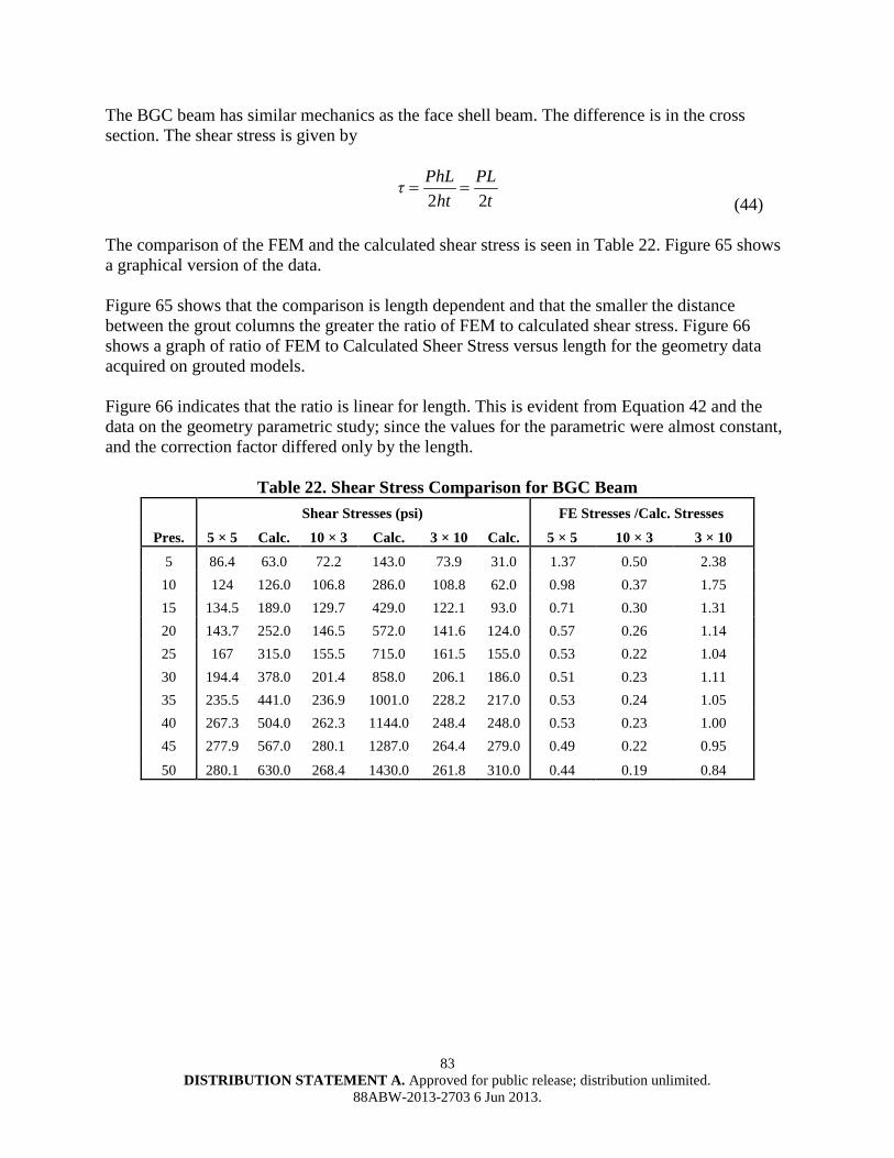
83 DISTRIBUTION STATEMENT A. Approved for public release; distribution unlimited.
88ABW-2013-2703 6 Jun 2013.
The BGC beam has similar mechanics as the face shell beam. The difference is in the cross section. The shear stress is given by
2 2PhL PLτ
ht t= =
(44) The comparison of the FEM and the calculated shear stress is seen in Table 22. Figure 65 shows a graphical version of the data. Figure 65 shows that the comparison is length dependent and that the smaller the distance between the grout columns the greater the ratio of FEM to calculated shear stress. Figure 66 shows a graph of ratio of FEM to Calculated Sheer Stress versus length for the geometry data acquired on grouted models. Figure 66 indicates that the ratio is linear for length. This is evident from Equation 42 and the data on the geometry parametric study; since the values for the parametric were almost constant, and the correction factor differed only by the length.
Table 22. Shear Stress Comparison for BGC Beam Shear Stresses (psi) FE Stresses /Calc. Stresses
Pres. 5 × 5 Calc. 10 × 3 Calc. 3 × 10 Calc. 5 × 5 10 × 3 3 × 10 5 86.4 63.0 72.2 143.0 73.9 31.0 1.37 0.50 2.38
10 124 126.0 106.8 286.0 108.8 62.0 0.98 0.37 1.75 15 134.5 189.0 129.7 429.0 122.1 93.0 0.71 0.30 1.31 20 143.7 252.0 146.5 572.0 141.6 124.0 0.57 0.26 1.14 25 167 315.0 155.5 715.0 161.5 155.0 0.53 0.22 1.04 30 194.4 378.0 201.4 858.0 206.1 186.0 0.51 0.23 1.11 35 235.5 441.0 236.9 1001.0 228.2 217.0 0.53 0.24 1.05 40 267.3 504.0 262.3 1144.0 248.4 248.0 0.53 0.23 1.00 45 277.9 567.0 280.1 1287.0 264.4 279.0 0.49 0.22 0.95
50 280.1 630.0 268.4 1430.0 261.8 310.0 0.44 0.19 0.84
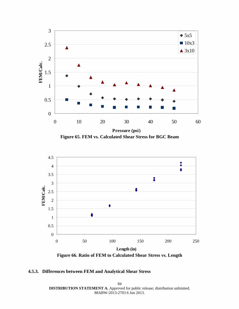
84 DISTRIBUTION STATEMENT A. Approved for public release; distribution unlimited.
88ABW-2013-2703 6 Jun 2013.
0
0.5
1
1.5
2
2.5
3
0 10 20 30 40 50 60
Pressure (psi)
FEM
/Cal
c.5x510x33x10
Figure 65. FEM vs. Calculated Shear Stress for BGC Beam
0
0.5
1
1.5
2
2.5
3
3.5
4
4.5
0 50 100 150 200 250
Length (in)
FEM
/Cal
c.
Figure 66. Ratio of FEM to Calculated Shear Stress vs. Length
4.5.3. Differences between FEM and Analytical Shear Stress
85 DISTRIBUTION STATEMENT A. Approved for public release; distribution unlimited.
88ABW-2013-2703 6 Jun 2013.
In both models, there are major differences between the shear stress calculated by FEM and calculated using beam models. The differences exist for a few different reasons. These reasons are (1) a lack of testing data on shear stresses in full-scale blast testing, (2) a lack of understanding of the mechanics in the breaching, (3) a lack of understanding of the concrete model used in FEM, (4) a lack of understanding in how to properly model mortar-block bond in highly dynamic loading, and (5) a lack of static testing to validate FEM modeling. More research is needed to understand most of the reasons the FEM and analytical models are not the same. However, there is a lack of testing data on shear stresses during blast loading, which is almost impossible to obtain. The rest can be found using static testing or dynamic testing. 4.6. Breaching Shear Design Equation
Finally, the shear strength, Vu, required by both models is
2
=uPLV (45)
The shear resistance, Vn, is given by
=n vmV Ctf (46) In order to prevent breaching, the nominal strength needs to be equal to or greater than the ultimate shear demand; this is given by
n≤uV V (47) or
2≤ vm
PL Ctf (48)
Solving for pressure results in
2
≤ vmCtfPL (49)
Using ACI 530.1 (ACI, 2011) and assuming that most building use type N mortar, the minimum compressive strength of the concrete block f’b is 2150 psi for a masonry assemblage with a compressive strength f’m of 1500 psi with Type N mortar. ACI 318 (ACI, 2011) gives the ultimate shear stress of concrete by
4 / 3 46 psivm bf = λ f' = (50) where λ = a correction factor for lightweight concrete (0.75). The shear stress strength is for plain concrete instead of masonry; this is because the masonry shear stress is built around
86 DISTRIBUTION STATEMENT A. Approved for public release; distribution unlimited.
88ABW-2013-2703 6 Jun 2013.
masonry-mortar bond and frictional sliding, not on the shear strength of concrete. Plugging Equation 50 into Equation 49 and solving for pressure gives
2 46 psiCtP
L× ×
≤ (51)
With Equation 51, a maximum pressure can be found for each block or section. Error! Reference source not found. shows the maximum pressure for a single block beam. Error! Reference source not found. shows the maximum for the BGC beams with length being based on maximum steel reinforcement spacing. For now, since the stress gradient in the FEM has not been calibrated with data from full-scale testing stress data, the correction factor is taken as 1 for now.
Table 23. Maximum Pressure for Single Block Beam
Single Block Beam L (in) t (in) P (psi)
6.0625 1.25 19
Table 24. Maximum Pressure for BGC Beams Between Grout Cells Beam
Nominal Block Size L (in) t (in) P (psi)
6-in 28 2.5 8.3 8-in 40 2.5 5.8
10-in 52 2.5 4.4 12-in 64 2.5 3.6 14-in 76 2.5 3.0
16-in 88 2.5 2.6
Only the single block beam provides a pressure that is independent of length between grout cells, geometry of the wall, and material properties of the blocks which is seen in the parametric study; the BGC beam is not independent of these. In addition, using the full-scale tests, the single block beam pressure matches closer to the results in the tests. Test 1 did breach, but not extensively, indicating that the pressure was around the cutoff between breaching and flexure. Test 2 and Test 3 had a more severe breaching response and the peak pressure was much higher than the single block beam and BGC beam pressures. Therefore, all masonry walls must be fully grouted if a pressure exceeding 28 psi is expected. Using UFC 3-340-02’s Figure 2-7, a minimum scaled standoff for a free air blast at sea level was obtained. This cutoff scaled standoff is 8.2 lb/ft1/3.
87 DISTRIBUTION STATEMENT A. Approved for public release; distribution unlimited.
88ABW-2013-2703 6 Jun 2013.
5. CONCLUSIONS AND RECOMMENDATIONS
5.1. Conclusions
Finite element models were developed to investigate the breaching phenomena of partially grouted concrete masonry walls that have been observed in recent blast load testing by the AFRL. The finite element model development methodology involved several steps: (1) creation of a FEM representing a partially grouted, reinforced CMU wall, (2) validation of the FEM against the full-scale dynamic test data, and (3) an input parameter study. The breaching behavior was found to be in the quasi-static regime, and therefore predominately a function of the peak reflected pressure. The parametric study showed that the shear stresses were largely independent of wall geometry, material properties, grouting geometry, and loading shape. It was demonstrated that the shear stresses were only dependent on the peak pressure applied to the face shell across a single cell. Engineering-level design equations were then derived that define the breach shear resistance provided. This resistance was found to be independent of wall geometry and only dependent on the clear span distance between webs, face shell thickness, peak pressure, and the shear strength of the masonry. For typical concrete masonry wall construction in the U.S., the peak pressure that would correlate to face shell shear breaching is approximately 20 psi. 5.2. Recommendations
Based on these findings, it is recommended that exterior CMU walls with a design peak pressure greater than 20 psi or a scaled standoff less than 10 lb/ft1/3 be fully grouted to preclude the potential for dangerous shear breaching failure modes. However, the results should be considered preliminary. This analytical investigation provided great insight into the causation of the shear breaching phenomena, but additional full-scale static and dynamic testing, combined with advanced modeling approaches illustrated in this investigation, is recommended to better understand CMU response and resistance to blast loading, with a focus on establishing a better understanding of breaching.

88 DISTRIBUTION STATEMENT A. Approved for public release; distribution unlimited.
88ABW-2013-2703 6 Jun 2013.
6. REFERENCES
1. American Concrete Institute (ACI) (2008). Building Code Requirements for Structural Concrete and Commentary, ACI 318-08, Farmington Hills, MI.
2. ACI (2011). Building Code Requirements and Specification for Masonry Structures, ACI 530-11, Farmington Hills, MI.
3. Atkinson R. H., Amadei, B. P., Saeb, S., and Sture, S. (1989). “Response of masonry bed joints in direct shear.” Journal of Structural Engineering, vol. 115 no. 9, pp. 2276-2296.
4. Biggs, J. M. (1964). “Introduction to Structural Dynamics,” McGraw-Hill, New York.
5. Browning IV, R. S. (2008). Resistance of multi-wythe insulated masonry subjected to impulse loads.” M.S. thesis, Auburn University, Auburn, AL.
6. Burnett, S., Gilbert, M., Molyneaus, T., Beattie, G., and Hobbs, B. (2006). “The performance of unreinforced masonry walls subjected to low velocity: finite element analysis.” International Journal of Impact Engineering, vol. 34, pp. 1433-1450.
7. Davidson, J. S., Moradi, L., and Dinan, R. J. (2006). “Selection of a material model for simulating concrete masonry walls subjected to blast.” AFRL-ML-TY-TR-2006-4521.
8. Davidson, J. S., Hoemann, J. M., Salim, H. H., and Shull, J. S. (2011). “Full-scale experimental evaluation of partially grouted, minimally reinforced CMU walls against blast demands.” AFRL-RX-TY-TR-2011-0025.
9. Dennis, S. T., Baylot, J. T., and Woodson, S. C. (2002). “Response of 1/4-scale concrete masonry unit walls to blast.” Journal of Engineering Mechanics, vol. 128, no. 2, pp. 134-142.
10. Department of Defense (2007), “DoD Minimum Antiterrorism Standards for Buildings,” UFC 4-010-01.
11. Department of Defense (2008). “Structures to Resist the Effects of Accidental Explosions,” UFC 3-340-02, Whole Building Design Guide, http://dod.wbdg.org/ (accessed Feb. 2011).
12. Drysdale, R. G., and Hamid, A. A. (2008). Masonry Structures Behavior and Design, 2nd Ed., The Masonry Society, Boulder, CO.
13. Eamon, C. D., Baylot, J. T., and O’Daniel, J. L. (2004). “Modeling concrete masonry walls subjected to explosive load.” Journal of Engineering Mechanics, vol. 130, no. 9, pp. 1098-1106.
14. Gilbert, M., Hobbs, B., and Molyneaux, T. C. K. (2002). “The performance of unreinforced masonry walls subjected to low-velocity impacts: mechanism analysis.” International Journal of Impact Engineering, vol. 27, pp. 253-275.
15. Hamid, A. A. and Drysdale, R. G. (1988). “Flexural tensile strength of concrete block masonry.” Journal of Structural Engineering. vol. 114, no. 1, pp. 50-66.
16. Krauthammer, T. (2008). “Pressure-impulse diagrams and their applications.” Modern Protective Structures. CRC Press, Boca Raton, FL, pp. 325-371.
17. Livermore Software Technology Corporation (LSTC) (2009). LS-DYNA Keyword User’s Manual.
89 DISTRIBUTION STATEMENT A. Approved for public release; distribution unlimited.
88ABW-2013-2703 6 Jun 2013.
18. Magallanes, J. M., Wu, Y., Malvar, L. J., and Crawford, J. E. (2010). “Recent Improvements to release III of the K&C concrete model.” 11th International LS-DYNA Users Conference. Livermore Software Technology Corporation, Livermore, CA, 3-37 - 3-48.
19. Martini, K. (1996). “Research in the out-of-plane behavior of unreinforced masonry.” Ancient Reconstruction of the Pompeii Forum, School of Architecture, University of Virginia.
20. Martini, K. (1998). “Finite element studies in the two-way out-of-plane failure of unreinforced masonry.” Ancient Reconstruction of the Pompeii Forum, School of Architecture, University of Virginia.
21. Moradi, L. G., Davidson, J. S., and Dinan, R. J. ( 2008). “Resistance of membrane retrofit concrete masonry walls to lateral pressure.” Journal of Performance of Constructed Facilities, vol. 22, no. 3, pp. 131-142.
22. Psilla, N. and Tassios, T. (2009). “Design of reinforced masonry walls under monotonic and cyclic loading.” Engineering Structures, vol. 31, pp. 935-945.
23. Salim H., Saucier A., Bell B, Hoemann J., Bewick B, Davidson J., Shull J. “Experimental Evaluation of Full-Scale NCMA Walls Under Uniform Pressure Using Vacuum,” draft report submitted to the Air Force Research Laboratory, July 2011.
24. Schwer, L. (2001) Draft, “Laboratory Tests for Characterizing Geomaterials” Livermore Software Technology Corporation, Livermore, California.
25. Schwer, L. (2005). “Simplified concrete modeling with Mat_Concrete_Damage_Rel3.” JRI LS-DYNA User Week. LSTC, Livermore, CA.
26. Smith, P. and Cormie, D. (2009) “Structural response to blast loading.” Blast Effects on Buildings. D. Cormie, G. Mays, and P. Smith, eds., Thomas Telford Limited, London, UK, pp. 80-102
27. Sudame, S. (2004). “Development of computational models and input sensitive study of polymer reinforced concrete masonry walls subjected to blast.” M.S. thesis, University of Alabama at Birmingham, Birmingham, AL
90 DISTRIBUTION STATEMENT A. Approved for public release; distribution unlimited.
88ABW-2013-2703 6 Jun 2013.
LIST OF SYMBOLS, ABBREVIATIONS, AND ACRONYMS
ACI American Concrete Institute AFRL Air Force Research Laboratory ASTM American Society for Testing and Materials BGC between grout cell CMU concrete masonry units D deflection gauge DoD Department of Defense DOF degree-of-freedom FEM finite element model FF free field gauge ft foot; feet in inch(es) IP incident pressure gauge ksi kips per square inch MDOF multiple degree-of-freedom MPa megapascal MPP massively parallel processor ms millisecond(s) MSJC Masonry Standards Joint Committee P-I pressure-impulse RP reflected pressure gauge SDOF single degree-of-freedom TNT trinitriotoluene UFC Unified Facility Criteria
Recommended