1

A Tutorial on Graph-Based SLAMGiorgio Grisetti Rainer Kummerle Cyrill Stachniss Wolfram Burgard

Department of Computer Science, University of Freiburg, 79110 Freiburg, Germany

Abstract—Being able to build a map of the environment andto simultaneously localize within this map is an essential skill formobile robots navigating in unknown environments in absenceof external referencing systems such as GPS. This so-calledsimultaneous localization and mapping (SLAM) problem hasbeen one of the most popular research topics in mobile roboticsfor the last two decades and efficient approaches for solving thistask have been proposed. One intuitive way of formulating SLAMis to use a graph whose nodes correspond to the poses of the robotat different points in time and whose edges represent constraintsbetween the poses. The latter are obtained from observationsof the environment or from movement actions carried out bythe robot. Once such a graph is constructed, the map can becomputed by finding the spatial configuration of the nodes thatis mostly consistent with the measurements modeled by theedges. In this paper, we provide an introductory descriptionto the graph-based SLAM problem. Furthermore, we discussa state-of-the-art solution that is based on least-squares errorminimization and exploits the structure of the SLAM problemsduring optimization. The goal of this tutorial is to enable thereader to implement the proposed methods from scratch.

I. I NTRODUCTION

To efficiently solve many tasks envisioned to be carried outby mobile robots including transportation, search and rescue,or automated vacuum cleaning robots need a map of theenvironment. The availability of an accurate map allows forthedesign of systems that can operate in complex environmentsonly based on their on-board sensors and without relyingon external reference system like, e.g., GPS. The acquisitionof maps of indoor environments, where typically no GPS isavailable, has been a major research focus in the roboticscommunity over the last decades. Learning maps under poseuncertainty is often referred to as the simultaneous localizationand mapping (SLAM) problem. In the literature, a large varietyof solutions to this problem is available. These approachescan be classified either as filtering or smoothing. Filteringapproaches model the problem as an on-line state estimationwhere the state of the system consists in thecurrent robot po-sition and the map. The estimate is augmented and refined byincorporating the new measurements as they become available.Popular techniques like Kalman and information filters [28],[3], particle filters [22], [12], [9], or information filters[7],[31] fall into this category. To highlight their incrementalnature, the filtering approaches are usually referred to ason-line SLAM methods. Conversely, smoothing approachesestimate the full trajectory of the robot from the full set ofmeasurements [21], [5], [27]. These approaches address theso-called full SLAM problem, and they typically rely on least-square error minimization techniques.

Figure 1 shows three examples of real robotic systemsthat use SLAM technology: an autonomous car, a tour-guide

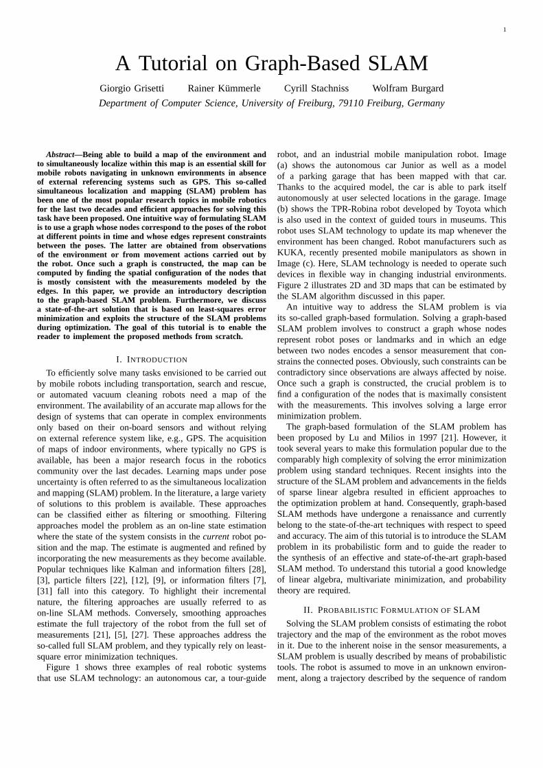
robot, and an industrial mobile manipulation robot. Image(a) shows the autonomous car Junior as well as a modelof a parking garage that has been mapped with that car.Thanks to the acquired model, the car is able to park itselfautonomously at user selected locations in the garage. Image(b) shows the TPR-Robina robot developed by Toyota whichis also used in the context of guided tours in museums. Thisrobot uses SLAM technology to update its map whenever theenvironment has been changed. Robot manufacturers such asKUKA, recently presented mobile manipulators as shown inImage (c). Here, SLAM technology is needed to operate suchdevices in flexible way in changing industrial environments.Figure 2 illustrates 2D and 3D maps that can be estimated bythe SLAM algorithm discussed in this paper.

An intuitive way to address the SLAM problem is viaits so-called graph-based formulation. Solving a graph-basedSLAM problem involves to construct a graph whose nodesrepresent robot poses or landmarks and in which an edgebetween two nodes encodes a sensor measurement that con-strains the connected poses. Obviously, such constraints can becontradictory since observations are always affected by noise.Once such a graph is constructed, the crucial problem is tofind a configuration of the nodes that is maximally consistentwith the measurements. This involves solving a large errorminimization problem.

The graph-based formulation of the SLAM problem hasbeen proposed by Lu and Milios in 1997 [21]. However, ittook several years to make this formulation popular due to thecomparably high complexity of solving the error minimizationproblem using standard techniques. Recent insights into thestructure of the SLAM problem and advancements in the fieldsof sparse linear algebra resulted in efficient approaches tothe optimization problem at hand. Consequently, graph-basedSLAM methods have undergone a renaissance and currentlybelong to the state-of-the-art techniques with respect to speedand accuracy. The aim of this tutorial is to introduce the SLAMproblem in its probabilistic form and to guide the reader tothe synthesis of an effective and state-of-the-art graph-basedSLAM method. To understand this tutorial a good knowledgeof linear algebra, multivariate minimization, and probabilitytheory are required.

II. PROBABILISTIC FORMULATION OF SLAM

Solving the SLAM problem consists of estimating the robottrajectory and the map of the environment as the robot movesin it. Due to the inherent noise in the sensor measurements, aSLAM problem is usually described by means of probabilistictools. The robot is assumed to move in an unknown environ-ment, along a trajectory described by the sequence of random

2

(a) (b) (c)

Fig. 1. Applications of SLAM technology. (a) An autonomous instrumented car developed at Stanford. This car can acquire maps by utilizing only itson-board sensors. These maps can be subsequently used for autonomous navigation. (b) The museum guide robot TPR-Robina developed by Toyota (picturecourtesy of Toyota Motor Company). This robot acquires a new map every time the museum is reconfigured. (c) The KUKA Concept robot “Omnirob”, amobile manipulator designed autonomously navigate and operate in the environment with the sole use of its on-board sensors (picture courtesy of KUKARoboter GmbH).

variablesx1:T = x1, . . . ,xT . While moving, it acquires asequence of odometry measurementsu1:T = u1, . . . ,uT and perceptions of the environmentz1:T = z1, . . . , zT .Solving the full SLAM problem consists of estimating theposterior probability of the robot’s trajectoryx1:T and themapm of the environment given all the measurements plusan initial positionx0:

p(x1:T ,m | z1:T ,u1:T ,x0). (1)

The initial positionx0 defines the position of the map andcan be chosen arbitrarily. For convenience of notation, in theremainder of this document we will omitx0. The posesx1:T

and the odometryu1:T are usually represented as 2D or 3Dtransformations inSE(2) or in SE(3), while the map can berepresented in different ways. Maps can be parametrized asa set of spatially located landmarks, by dense representationslike occupancy grids, surface maps, or by raw sensor measure-ments. The choice of a particular map representation dependson the sensors used, on the characteristics of the environment,and on the estimation algorithm. Landmark maps [28], [22] areoften preferred in environments where locally distinguishablefeatures can be identified and especially when cameras areused. In contrast, dense representations [33], [12], [9] areusually used in conjunction with range sensors. Independentlyof the type of the representation, the map is defined by themeasurements and the locations where these measurementshave been acquired [17], [18]. Figure 2 illustrates three typicaldense map representations for 3D and 2D: multilevel surfacemaps, point clouds and occupancy grids. Figure 3 shows atypical 2D landmark based map.

Estimating the posterior given in (1) involves operating inhigh dimensional state spaces. This would not be tractable ifthe SLAM problem would not have a well defined structure.This structure arises from certain and commonly done assump-tions, namely the static world assumption and the Markovassumption. A convenient way to describe this structure is viathe dynamic Bayesian network (DBN) depicted in Figure 4.A Bayesian network is a graphical model that describes astochastic process as a directed graph. The graph has one nodefor each random variable in the process, and a directed edge (or

-20

-10

0

10

20

30

-50 -40 -30 -20 -10 0 10 20

landmarkstrajectory

Fig. 3. Landmark based maps acquired at the German Aerospace Center. Inthis setup the landmarks consist in white circles painted on the ground thatare detected by the robot through vision, as shown in the leftimage. The rightimage illustrates the trajectory of the robot and the estimated positions of thelandmarks. These images are courtesy of Udo Frese and Christoph Hertzberg.

x0 x1 xt−1 xt xT

u1 ut−1 ut uT

z1 zt−1 zt zT

m

Fig. 4. Dynamic Bayesian Network of the SLAM process.

arrow) between two nodes models a conditional dependencebetween them.

In Figure 4, one can distinguish blue/gray nodes indicatingthe observed variables (herez1:T andu1:T ) and white nodeswhich are the hidden variables. The hidden variablesx1:T

and m model the robot’s trajectory and the map of theenvironment. The connectivity of the DBN follows a recurrent

3

(a) (b) (c)

Fig. 2. (a) A 3D map of the Stanford parking garage acquired with an instrumented car (bottom), and the corresponding satellite view (top). This map hasbeen subsequently used to realize an autonomous parking behavior. (b) Point cloud map acquired at the university of Freiburg (courtesy of Kai. M. Wurm)and relative satellite image. (c) Occupancy grid map acquiredat the hospital of Freiburg. Top: a bird’s eye view of the area, bottom: the occupancy gridrepresentation. The gray areas represent unobserved regions, the white part represents traversable space while the black points indicate occupied regions.

pattern characterized by the state transition model and by theobservation model. The transition modelp(xt | xt−1,ut) isrepresented by the two edges leading toxt and represents theprobability that the robot at timet is in xt given that at timet − 1 it was in xt and it acquired an odometry measurementut.

The observation modelp(zt | xt,mt) models the probabil-ity of performing the observationzt given that the robot is atlocationxt in the map. It is represented by the arrows enteringin zt. The exteroceptive observationzt depends only on thecurrent locationxt of the robot and on the (static) mapm.Expressing SLAM as a DBN highlights its temporal structure,and therefore this formalism is well suited to describe filteringprocesses that can be used to tackle the SLAM problem.

An alternative representation to the DBN is via the so-called“graph-based” or “network-based” formulation of the SLAMproblem, that highlights the underlying spatial structure. Ingraph-based SLAM, the poses of the robot are modeled bynodes in a graph and labeled with their position in theenvironment [21], [18]. Spatial constraints between posesthatresult from observationszt or from odometry measurementsut are encoded in the edges between the nodes. More indetail, a graph-based SLAM algorithm constructs a graph outof the raw sensor measurements. Each node in the graphrepresents a robot position and a measurement acquired atthat position. An edge between two nodes represents a spatialconstraint relating the two robot poses. A constraint consistsin a probability distribution over the relative transformationsbetween the two poses. These transformations are either odom-etry measurements between sequential robot positions or aredetermined by aligning the observations acquired at the tworobot locations. Once the graph is constructed one seeks tofind the configuration of the robot poses that best satisfiesthe constraints. Thus, in graph-based SLAM the problemis decoupled in two tasks: constructing the graph from theraw measurements (graph construction), determining the mostlikely configuration of the poses given the edges of the graph(graph optimization). The graph construction is usually called

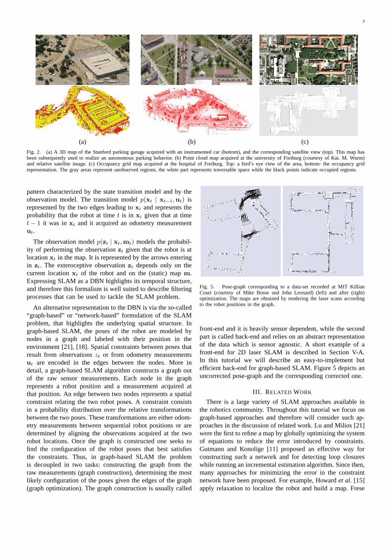
Fig. 5. Pose-graph corresponding to a data-set recorded at MIT KillianCourt (courtesy of Mike Bosse and John Leonard) (left) and after (right)optimization. The maps are obtained by rendering the laser scans accordingto the robot positions in the graph.

front-end and it is heavily sensor dependent, while the secondpart is called back-end and relies on an abstract representationof the data which is sensor agnostic. A short example of afront-end for 2D laser SLAM is described in Section V-A.In this tutorial we will describe an easy-to-implement butefficient back-end for graph-based SLAM. Figure 5 depicts anuncorrected pose-graph and the corresponding corrected one.

III. R ELATED WORK

There is a large variety of SLAM approaches available inthe robotics community. Throughout this tutorial we focus ongraph-based approaches and therefore will consider such ap-proaches in the discussion of related work. Lu and Milios [21]were the first to refine a map by globally optimizing the systemof equations to reduce the error introduced by constraints.Gutmann and Konolige [11] proposed an effective way forconstructing such a network and for detecting loop closureswhile running an incremental estimation algorithm. Since then,many approaches for minimizing the error in the constraintnetwork have been proposed. For example, Howardet al. [15]apply relaxation to localize the robot and build a map. Frese

4

et al. [8] propose a variant of Gauss-Seidel relaxation calledmulti-level relaxation (MLR). It applies relaxation at differentresolutions. Dellaert and Kaess [5] were the first to exploitsparse matrix factorizations to solve the linearized problemin off-line SLAM. Subsequently Kaesset al. [16] presentediSAM, an on-line version that exploits partial reorderingstocompute the sparse factorization.

Recently, Konoligeet al. [19] proposed an open-sourceimplementation of a pose-graph method that constructs thelinearized system in an efficient way. Olsonet al. [27] pre-sented an efficient optimization approach which is based onthe stochastic gradient descent and can efficiently correctevenlarge pose-graphs. Grisettiet al. proposed an extension ofOlson’s approach that uses a tree parametrization of the nodesin 2D and 3D. In this way, they increase the convergencespeed [10].

GraphSLAM [32] applies variable elimination techniques toreduce the dimensionality of the optimization problem. TheATLAS framework [2] constructs a two-level hierarchy ofgraphs and employs a Kalman filter to construct the bottomlevel. Then, a global optimization approach aligns the localmaps at the second level. Similar to ATLAS, Estradaet al.proposed Hierarchical SLAM [6] as a technique for usingindependent local maps.

Most optimization techniques focus on computing the bestmap given the constraints and are called SLAM back-ends.In contrast to that, SLAM front-ends seek to interpret thesensor data to obtain the constraints that are the basis forthe optimization approaches. Olson [25], for example, pre-sented a front-end with outlier rejection based on spectralclustering. For making data associations in the SLAM front-ends statistical tests such as theχ2 test or joint compatibilitytest [23] are often applied. The work of Nuchter et al. [24]aims at building an integrated SLAM system for 3D mapping.The main focus lies on the SLAM front-end for findingconstraints. For optimization, a variant of the approach ofLu and Milios [21] for 3D settings is applied. The methodsproposed in this paper can be effectively applied to all thesefront-ends.

IV. GRAPH-BASED SLAM

A graph-based SLAM approach constructs a simplified esti-mation problem by abstracting the raw sensor measurements.These raw measurements are replaced by the edges in thegraph which can then be seen as “virtual measurements”.More in detail an edge between two nodes is labeled witha probability distribution over the relative locations of the twoposes, conditioned to their mutual measurements. In general,the observation modelp(zt | xt,mt) is multi-modal andtherefore the Gaussian assumption does not hold. This meansthat a single observationzt might result in multiple potentialedges connecting different poses in the graph and the graphconnectivity needs itself to be described as a probabilitydistribution. Directly dealing with this multi-modality in theestimation process would lead to a combinatorial explosionofthe complexity. As a result of that, most practical approachesrestrict the estimate to the most likely topology. Thus, one

x1

x2 x3

xixj

xt−1xt

xT

〈eij ,Ωij〉

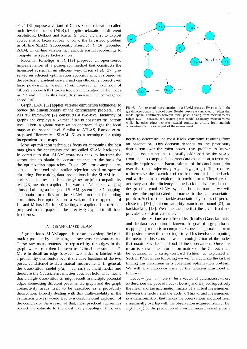
Fig. 6. A pose-graph representation of a SLAM process. Everynode in thegraph corresponds to a robot pose. Nearby poses are connected by edges thatmodel spatial constraints between robot poses arising from measurements.Edgeset−1 t between consecutive poses model odometry measurements,while the other edges represent spatial constraints arising from multipleobservations of the same part of the environment.

needs to determine the most likely constraint resulting froman observation. This decision depends on the probabilitydistribution over the robot poses. This problem is knownas data association and is usually addressed by the SLAMfront-end. To compute the correct data-association, a front-endusually requires a consistent estimate of the conditional priorover the robot trajectoryp(x1:T | z1:T ,u1:T ). This requiresto interleave the execution of the front-end and of the back-end while the robot explores the environment. Therefore, theaccuracy and the efficiency of the back-end is crucial to thedesign of a good SLAM system. In this tutorial, we willnot describe sophisticated approaches to the data associationproblem. Such methods tackle association by means of spectralclustering [27], joint compatibility branch and bound [23], orbacktracking [13]. We rather assume that the given front-endprovides consistent estimates.

If the observations are affected by (locally) Gaussian noiseand the data association is known, the goal of a graph-basedmapping algorithm is to compute a Gaussian approximation ofthe posterior over the robot trajectory. This involves computingthe mean of this Gaussian as the configuration of the nodesthat maximizes the likelihood of the observations. Once thismean is known the information matrix of the Gaussian canbe obtained in a straightforward fashion, as explained inSection IV-B. In the following we will characterize the taskoffinding this maximum as a constraint optimization problem.We will also introduce parts of the notation illustrated inFigure 6.

Let x = (x1, . . . ,xT )T be a vector of parameters, where

xi describes the pose of nodei. Let zij andΩij be respectivelythe mean and the information matrix of a virtual measurementbetween the nodei and the nodej. This virtual measurementis a transformation that makes the observations acquired fromi maximally overlap with the observation acquired fromj. Letzij(xi,xj) be the prediction of a virtual measurement given a

5

xi

xj

zij

zij

Ωij

eij(xi,xj)

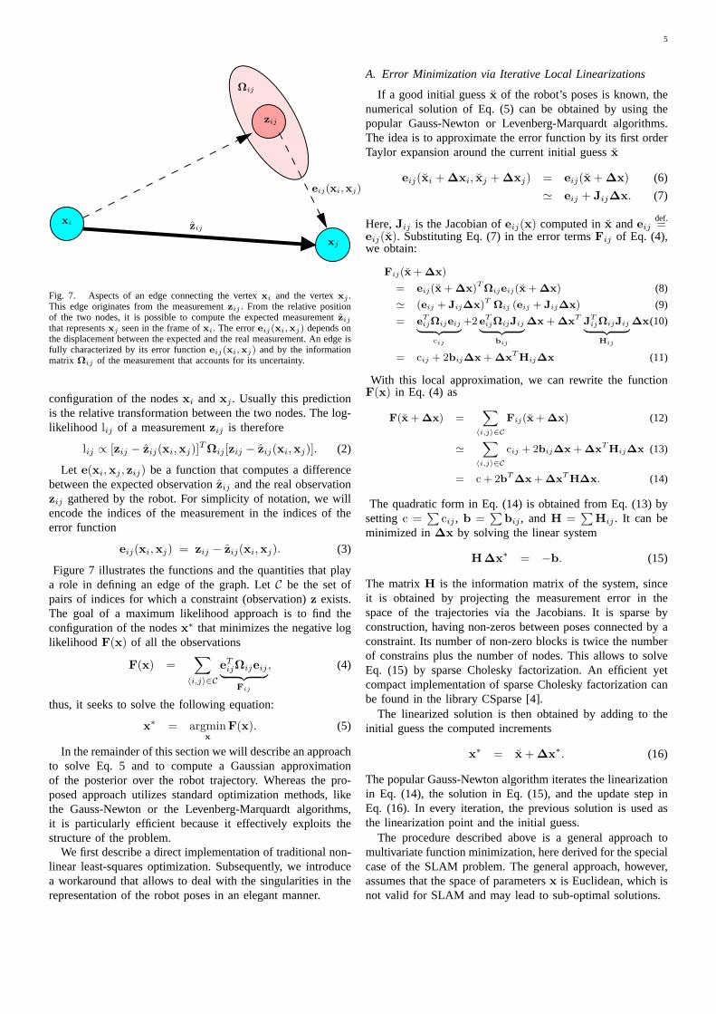
Fig. 7. Aspects of an edge connecting the vertexxi and the vertexxj .This edge originates from the measurementzij . From the relative positionof the two nodes, it is possible to compute the expected measurement zijthat representsxj seen in the frame ofxi. The erroreij(xi,xj) depends onthe displacement between the expected and the real measurement. An edge isfully characterized by its error functioneij(xi,xj) and by the informationmatrix Ωij of the measurement that accounts for its uncertainty.

configuration of the nodesxi andxj . Usually this predictionis the relative transformation between the two nodes. The log-likelihood lij of a measurementzij is therefore

lij ∝ [zij − zij(xi,xj)]TΩij [zij − zij(xi,xj)]. (2)

Let e(xi,xj , zij) be a function that computes a differencebetween the expected observationzij and the real observationzij gathered by the robot. For simplicity of notation, we willencode the indices of the measurement in the indices of theerror function

eij(xi,xj) = zij − zij(xi,xj). (3)

Figure 7 illustrates the functions and the quantities that playa role in defining an edge of the graph. LetC be the set ofpairs of indices for which a constraint (observation)z exists.The goal of a maximum likelihood approach is to find theconfiguration of the nodesx∗ that minimizes the negative loglikelihood F(x) of all the observations

F(x) =∑

〈i,j〉∈C

eTijΩijeij︸ ︷︷ ︸

Fij

, (4)

thus, it seeks to solve the following equation:

x∗ = argminx

F(x). (5)

In the remainder of this section we will describe an approachto solve Eq. 5 and to compute a Gaussian approximationof the posterior over the robot trajectory. Whereas the pro-posed approach utilizes standard optimization methods, likethe Gauss-Newton or the Levenberg-Marquardt algorithms,it is particularly efficient because it effectively exploits thestructure of the problem.

We first describe a direct implementation of traditional non-linear least-squares optimization. Subsequently, we introducea workaround that allows to deal with the singularities in therepresentation of the robot poses in an elegant manner.

A. Error Minimization via Iterative Local Linearizations

If a good initial guessx of the robot’s poses is known, thenumerical solution of Eq. (5) can be obtained by using thepopular Gauss-Newton or Levenberg-Marquardt algorithms.The idea is to approximate the error function by its first orderTaylor expansion around the current initial guessx

eij(xi +∆xi, xj +∆xj) = eij(x+∆x) (6)

≃ eij + Jij∆x. (7)

Here,Jij is the Jacobian ofeij(x) computed inx andeijdef.=

eij(x). Substituting Eq. (7) in the error termsFij of Eq. (4),we obtain:

Fij(x+∆x)

= eij(x+∆x)TΩijeij(x+∆x) (8)

≃ (eij + Jij∆x)T Ωij (eij + Jij∆x) (9)

= eTijΩijeij

︸ ︷︷ ︸

cij

+2 eTijΩijJij

︸ ︷︷ ︸

bij

∆x+∆xTJTijΩijJij

︸ ︷︷ ︸

Hij

∆x(10)

= cij + 2bij∆x+∆xTHij∆x (11)

With this local approximation, we can rewrite the functionF(x) in Eq. (4) as

F(x+∆x) =∑

〈i,j〉∈C

Fij(x+∆x) (12)

≃∑

〈i,j〉∈C

cij + 2bij∆x+∆xTHij∆x (13)

= c + 2bT∆x+∆x

TH∆x. (14)

The quadratic form in Eq. (14) is obtained from Eq. (13) bysetting c =

∑cij , b =

∑bij , andH =

∑Hij . It can be

minimized in∆x by solving the linear system

H∆x∗ = −b. (15)

The matrixH is the information matrix of the system, sinceit is obtained by projecting the measurement error in thespace of the trajectories via the Jacobians. It is sparse byconstruction, having non-zeros between poses connected byaconstraint. Its number of non-zero blocks is twice the numberof constrains plus the number of nodes. This allows to solveEq. (15) by sparse Cholesky factorization. An efficient yetcompact implementation of sparse Cholesky factorization canbe found in the library CSparse [4].

The linearized solution is then obtained by adding to theinitial guess the computed increments

x∗ = x+∆x∗. (16)

The popular Gauss-Newton algorithm iterates the linearizationin Eq. (14), the solution in Eq. (15), and the update step inEq. (16). In every iteration, the previous solution is used asthe linearization point and the initial guess.

The procedure described above is a general approach tomultivariate function minimization, here derived for the specialcase of the SLAM problem. The general approach, however,assumes that the space of parametersx is Euclidean, which isnot valid for SLAM and may lead to sub-optimal solutions.

6

B. Considerations about the Structure of the Linearized Sys-tem

According to Eq. (14), the matrixH and the vectorb areobtained by summing up a set of matrices and vectors, one forevery constraint. Every constraint will contribute to the systemwith an addend term. Thestructureof this addend depends onthe Jacobian of the error function. Since the error functionof a constraint depends only on the values of two nodes, theJacobian in Eq. (7) has the following form:

Jij =

0 · · ·0 Aij

︸︷︷︸

node i

0 · · ·0 Bij︸︷︷︸

node j

0 · · ·0

. (17)

HereAij andBij are the derivatives of the error function withrespect toxi andxj . From Eq. (10) we obtain the followingstructure for the block matrixHij :

Hij =

. . .AT

ijΩijAij · · · ATijΩijBij

.... . .

...BT

ijΩijAij · · · BTijΩijBij

. ..

(18)

bij =

...AT

ijΩijeij...

BTijΩijeij

...

(19)

For simplicity of notation we omitted the zero blocks.Algorithm 1 summarizes an iterative Gauss-Newton proce-

dure to determine both the mean and the information matrixof the posterior over the robot poses. Since most of thestructures in the system are sparse, we recommend to usememory efficient representations to store the HessianH ofthe system. Since the structure of the Hessian is known inadvance from the connectivity of the graph, we recommend topre-allocate the Hessian once at the beginning of the iterationsand to update it in place by looping over all edges whenevera new linearization is required. Each edge contributes to theblocks H[ii], H[ij], H[ji], and H[jj] and to the blocksb[i]

andb[j] of the coefficient vector. An additional optimizationis to compute only the upper triangular part ofH, since itis symmetric. Note that the error of a constrainteij dependsonly on the relative position of the connected posesxi andxj . Accordingly, the errorF(x) of a particular configurationof the posesx is invariant under a rigid transformation of allthe poses. This results in Eq. 15 being under determined. Tonumerically solve this system it is therefore common practiceto constrain one of the increments∆xk to be zero. This can bedone by adding the identity matrix to thekth diagonal blockH[kk]. Without loss of generality in Algorithm 1 we fix thefirst nodex1. An alternative way to fix a particular node ofthe pose-graph consists in suppressing thekth block row andthe kth block column of the linear system in Eq. 15.

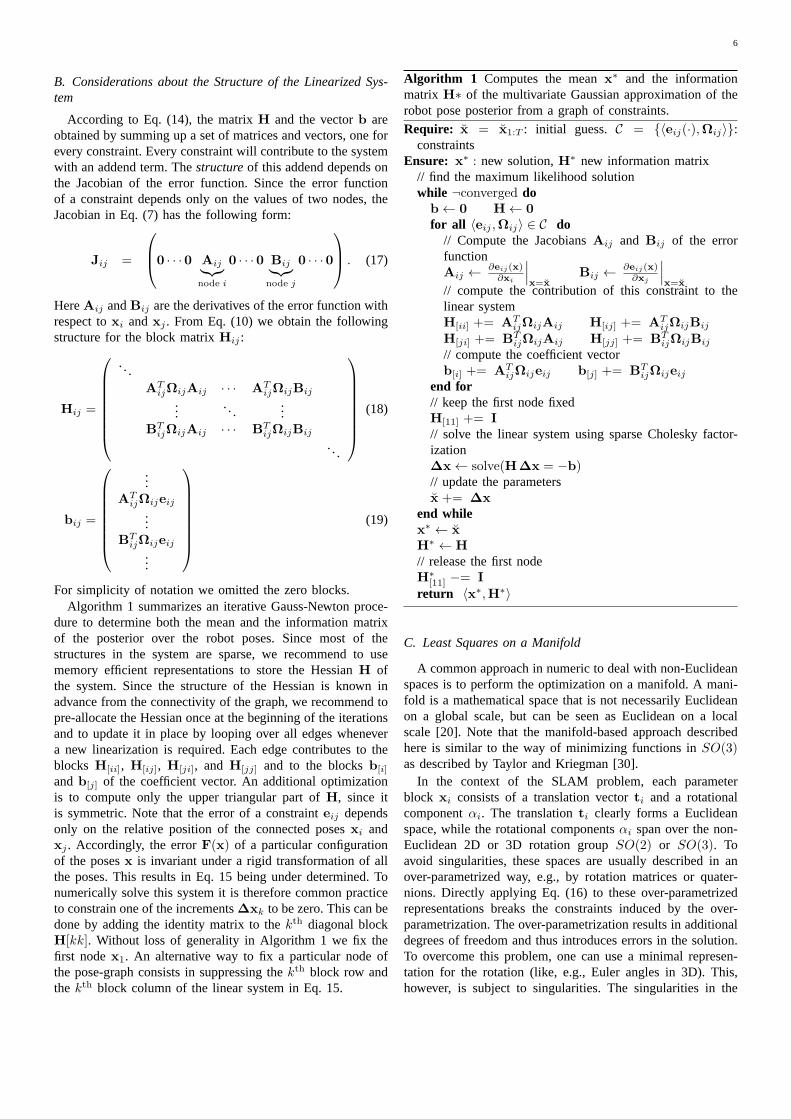
Algorithm 1 Computes the meanx∗ and the informationmatrix H∗ of the multivariate Gaussian approximation of therobot pose posterior from a graph of constraints.

Require: x = x1:T : initial guess. C = 〈eij(·),Ωij〉:constraints

Ensure: x∗ : new solution,H∗ new information matrix// find the maximum likelihood solutionwhile ¬converged dob← 0 H← 0

for all 〈eij ,Ωij〉 ∈ C do// Compute the JacobiansAij and Bij of the errorfunctionAij ←

∂eij(x)∂xi

∣∣∣x=x

Bij ←∂eij(x)∂xj

∣∣∣x=x

// compute the contribution of this constraint to thelinear systemH[ii] += AT

ijΩijAij H[ij] += ATijΩijBij

H[ji] += BTijΩijAij H[jj] += BT

ijΩijBij

// compute the coefficient vectorb[i] += AT

ijΩijeij b[j] += BTijΩijeij

end for// keep the first node fixedH[11] += I

// solve the linear system using sparse Cholesky factor-ization∆x← solve(H∆x = −b)// update the parametersx += ∆x

end whilex∗ ← x

H∗ ← H

// release the first nodeH∗

[11] −= I

return 〈x∗,H∗〉

C. Least Squares on a Manifold

A common approach in numeric to deal with non-Euclideanspaces is to perform the optimization on a manifold. A mani-fold is a mathematical space that is not necessarily Euclideanon a global scale, but can be seen as Euclidean on a localscale [20]. Note that the manifold-based approach describedhere is similar to the way of minimizing functions inSO(3)as described by Taylor and Kriegman [30].

In the context of the SLAM problem, each parameterblock xi consists of a translation vectorti and a rotationalcomponentαi. The translationti clearly forms a Euclideanspace, while the rotational componentsαi span over the non-Euclidean 2D or 3D rotation groupSO(2) or SO(3). Toavoid singularities, these spaces are usually described inanover-parametrized way, e.g., by rotation matrices or quater-nions. Directly applying Eq. (16) to these over-parametrizedrepresentations breaks the constraints induced by the over-parametrization. The over-parametrization results in additionaldegrees of freedom and thus introduces errors in the solution.To overcome this problem, one can use a minimal represen-tation for the rotation (like, e.g., Euler angles in 3D). This,however, is subject to singularities. The singularities inthe

7

2D case can be easily recovered by normalizing the angle,however in 3D this procedure is not straightforward.

An alternative idea is to consider the underlying space asa manifold and to define an operator⊞ that maps a localvariation ∆x in the Euclidean space to a variation on themanifold,∆x 7→ x⊞∆x. We refer the reader to the work ofHertzberg [14] for the mathematical details. With this operator,a new error function can be defined as

eij(∆xi,∆xj)def.= eij(xi ⊞∆xi, xj ⊞∆xj) (20)

= eij(x⊞∆x) ≃ eij + Jij∆x,(21)

where x spans over the original over-parametrized space,for instance quaternions. The term∆x is a small incrementaround the original positionx and is expressed in a minimalrepresentation.

As an example, in 3D SLAM a good choice of theparametrization of the rotations is thevector partof the unitquaternion. In more detail, one can represent the increments∆x as 6D vectors∆x

T = (∆tTqT ), where∆t denotes

the translation andqT = (∆qx ∆qy ∆qz)T is the vector

part of the unit quaternion representing the 3D rotation.Conversely,xT = (tT qT ) uses a quaternionq to encode therotational part. Thus, the operator⊞ can be expressed by firstconverting∆q to a full quaternion∆q and then applying thetransformation∆xT = (∆tT ∆qT ) to x. In the equationsdescribing the error minimization, these operations can nicelybe encapsulated by the⊞ operator. The JacobianJij can beexpressed by

Jij =∂eij(x⊞∆x)

∂∆x

∣∣∣∣∆x=0

. (22)

Since in the previous equatione depends only on∆xi and∆xj we can further expand it as follows:

Jij (23)

=

· · ·∂eij(x⊞∆x)

∂∆xi

∣∣∣∣∆x=0

︸ ︷︷ ︸

Aij

· · ·∂eij(x⊞∆x)

∂∆xj

∣∣∣∣∆x=0

︸ ︷︷ ︸

Bij

· · ·

Using the rule for the partial derivatives and exploiting thefact that the Jacobian is evaluated in∆x = 0, the non-zeroblocks become:

∂eij(x⊞∆xi)

∂∆xi

=∂eij(x)

∂xi︸ ︷︷ ︸

Aij

·xi ⊞∆xi

∂∆xi

∣∣∣∣∆x=0

︸ ︷︷ ︸

Mi

(24)

∂eij(x⊞∆xj)

∂∆xj

=∂eij(x)

∂xj︸ ︷︷ ︸

Bij

·xj ⊞∆xj

∂∆xj

∣∣∣∣∆x=0

︸ ︷︷ ︸

Mj

(25)

Accordingly, one can easily derive from the Jacobian notdefined on a manifold of Eq. 17 a Jacobian on a manifoldjust by multiplying its non-zero blocks with the derivativeofthe⊞ operator computed inxi and xj .

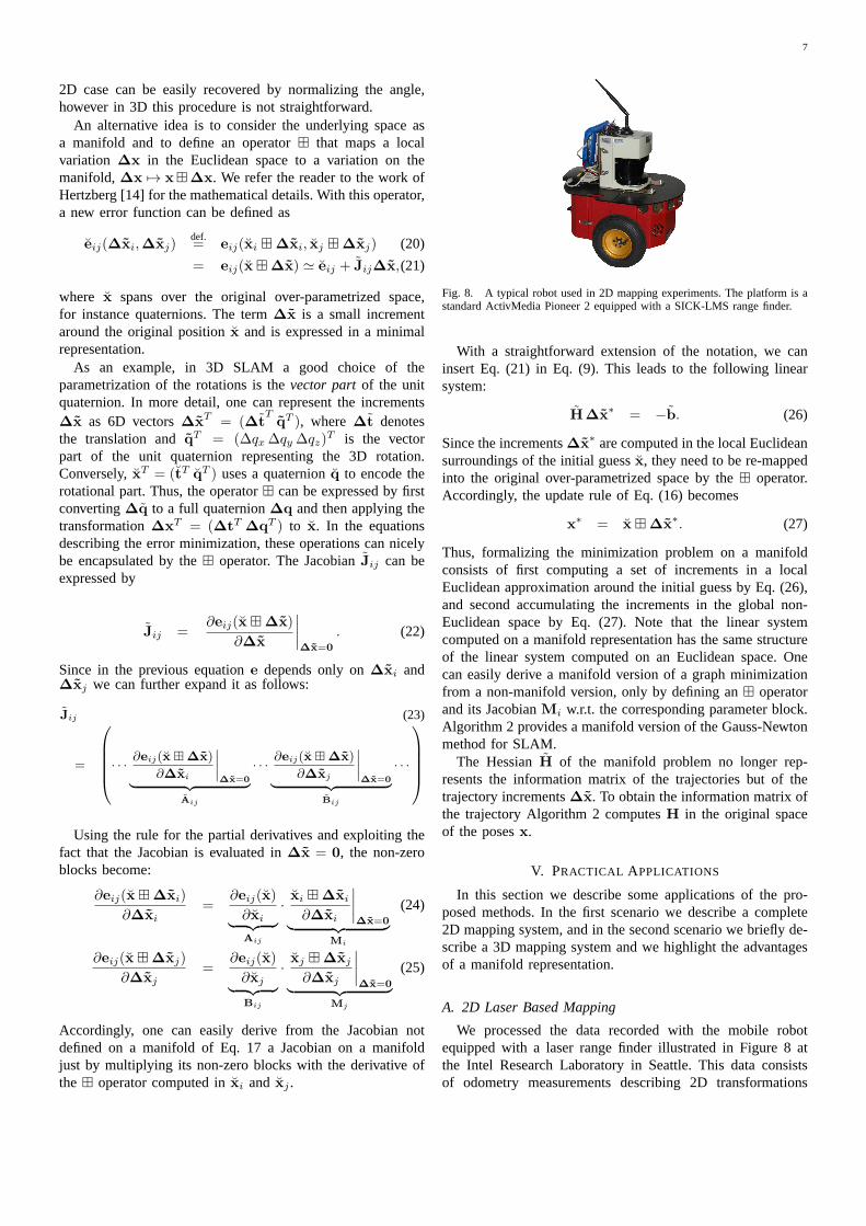
Fig. 8. A typical robot used in 2D mapping experiments. The platform is astandard ActivMedia Pioneer 2 equipped with a SICK-LMS range finder.

With a straightforward extension of the notation, we caninsert Eq. (21) in Eq. (9). This leads to the following linearsystem:

H∆x∗ = −b. (26)

Since the increments∆x∗ are computed in the local Euclidean

surroundings of the initial guessx, they need to be re-mappedinto the original over-parametrized space by the⊞ operator.Accordingly, the update rule of Eq. (16) becomes

x∗ = x⊞∆x∗. (27)

Thus, formalizing the minimization problem on a manifoldconsists of first computing a set of increments in a localEuclidean approximation around the initial guess by Eq. (26),and second accumulating the increments in the global non-Euclidean space by Eq. (27). Note that the linear systemcomputed on a manifold representation has the same structureof the linear system computed on an Euclidean space. Onecan easily derive a manifold version of a graph minimizationfrom a non-manifold version, only by defining an⊞ operatorand its JacobianMi w.r.t. the corresponding parameter block.Algorithm 2 provides a manifold version of the Gauss-Newtonmethod for SLAM.

The HessianH of the manifold problem no longer rep-resents the information matrix of the trajectories but of thetrajectory increments∆x. To obtain the information matrix ofthe trajectory Algorithm 2 computesH in the original spaceof the posesx.

V. PRACTICAL APPLICATIONS

In this section we describe some applications of the pro-posed methods. In the first scenario we describe a complete2D mapping system, and in the second scenario we briefly de-scribe a 3D mapping system and we highlight the advantagesof a manifold representation.

A. 2D Laser Based Mapping

We processed the data recorded with the mobile robotequipped with a laser range finder illustrated in Figure 8 atthe Intel Research Laboratory in Seattle. This data consistsof odometry measurements describing 2D transformations

8

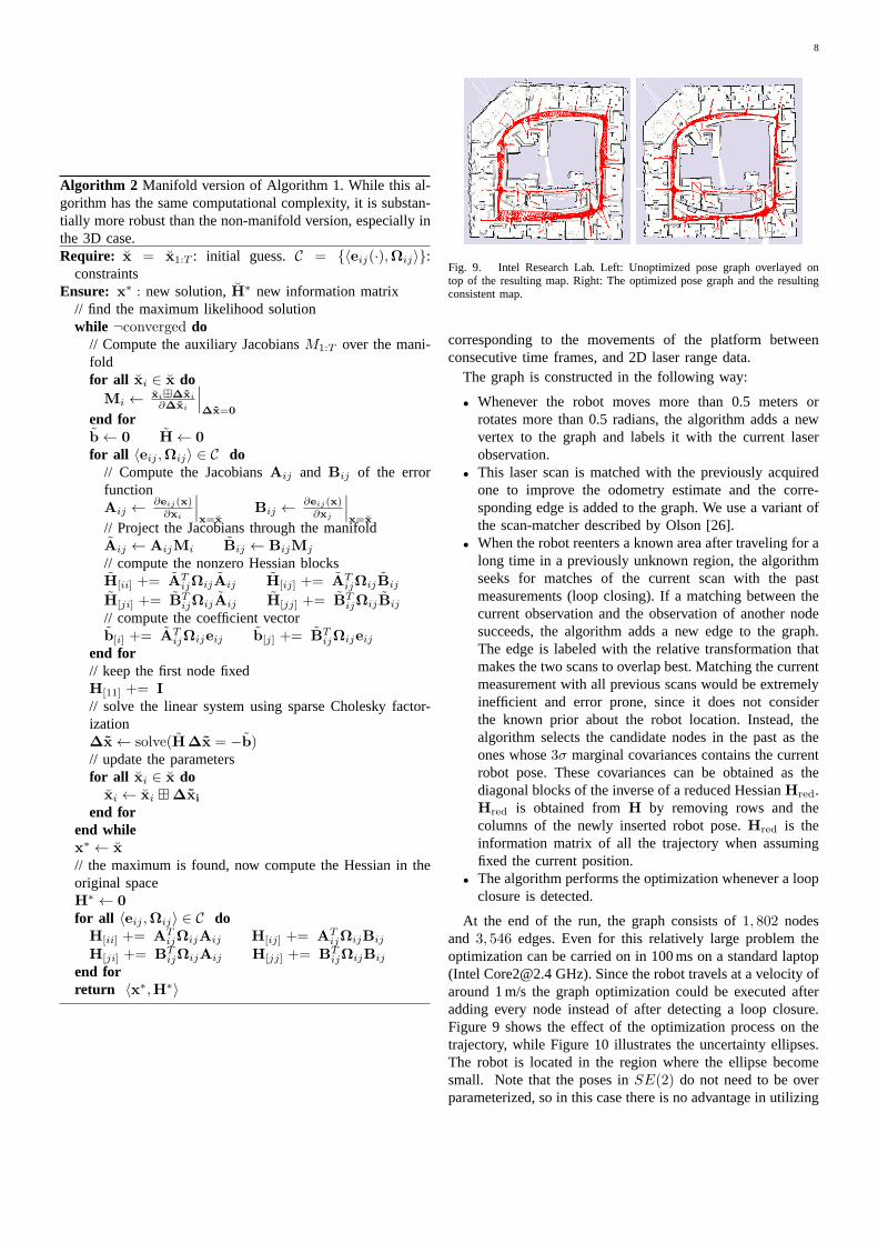
Algorithm 2 Manifold version of Algorithm 1. While this al-gorithm has the same computational complexity, it is substan-tially more robust than the non-manifold version, especially inthe 3D case.Require: x = x1:T : initial guess. C = 〈eij(·),Ωij〉:

constraintsEnsure: x∗ : new solution,H∗ new information matrix

// find the maximum likelihood solutionwhile ¬converged do

// Compute the auxiliary JacobiansM1:T over the mani-foldfor all xi ∈ x doMi ←

xi⊞∆xi

∂∆xi

∣∣∣∆x=0

end forb← 0 H← 0

for all 〈eij ,Ωij〉 ∈ C do// Compute the JacobiansAij and Bij of the errorfunctionAij ←

∂eij(x)∂xi

∣∣∣x=x

Bij ←∂eij(x)∂xj

∣∣∣x=x

// Project the Jacobians through the manifoldAij ← AijMi Bij ← BijMj

// compute the nonzero Hessian blocksH[ii] += AT

ijΩijAij H[ij] += ATijΩijBij

H[ji] += BTijΩijAij H[jj] += BT

ijΩijBij

// compute the coefficient vectorb[i] += AT

ijΩijeij b[j] += BTijΩijeij

end for// keep the first node fixedH[11] += I

// solve the linear system using sparse Cholesky factor-ization∆x← solve(H∆x = −b)// update the parametersfor all xi ∈ x doxi ← xi ⊞∆xi

end forend whilex∗ ← x

// the maximum is found, now compute the Hessian in theoriginal spaceH∗ ← 0

for all 〈eij ,Ωij〉 ∈ C doH[ii] += AT

ijΩijAij H[ij] += ATijΩijBij

H[ji] += BTijΩijAij H[jj] += BT

ijΩijBij

end forreturn 〈x∗,H∗〉

Fig. 9. Intel Research Lab. Left: Unoptimized pose graph overlayed ontop of the resulting map. Right: The optimized pose graph and the resultingconsistent map.

corresponding to the movements of the platform betweenconsecutive time frames, and 2D laser range data.

The graph is constructed in the following way:

• Whenever the robot moves more than 0.5 meters orrotates more than 0.5 radians, the algorithm adds a newvertex to the graph and labels it with the current laserobservation.

• This laser scan is matched with the previously acquiredone to improve the odometry estimate and the corre-sponding edge is added to the graph. We use a variant ofthe scan-matcher described by Olson [26].

• When the robot reenters a known area after traveling for along time in a previously unknown region, the algorithmseeks for matches of the current scan with the pastmeasurements (loop closing). If a matching between thecurrent observation and the observation of another nodesucceeds, the algorithm adds a new edge to the graph.The edge is labeled with the relative transformation thatmakes the two scans to overlap best. Matching the currentmeasurement with all previous scans would be extremelyinefficient and error prone, since it does not considerthe known prior about the robot location. Instead, thealgorithm selects the candidate nodes in the past as theones whose3σ marginal covariances contains the currentrobot pose. These covariances can be obtained as thediagonal blocks of the inverse of a reduced HessianHred.Hred is obtained fromH by removing rows and thecolumns of the newly inserted robot pose.Hred is theinformation matrix of all the trajectory when assumingfixed the current position.

• The algorithm performs the optimization whenever a loopclosure is detected.

At the end of the run, the graph consists of1, 802 nodesand 3, 546 edges. Even for this relatively large problem theoptimization can be carried on in 100 ms on a standard laptop(Intel Core2@2.4 GHz). Since the robot travels at a velocityofaround 1 m/s the graph optimization could be executed afteradding every node instead of after detecting a loop closure.Figure 9 shows the effect of the optimization process on thetrajectory, while Figure 10 illustrates the uncertainty ellipses.The robot is located in the region where the ellipse becomesmall. Note that the poses inSE(2) do not need to be overparameterized, so in this case there is no advantage in utilizing

9

Fig. 10. Pose uncertainty estimate for a real-world data set.

manifolds.

B. 3D Laser Based Mapping

Extending to 3D the SLAM algorithm presented in theprevious section is rather straightforward. One has only toreplace the 2D scan matching and loop closure detectionwith their 3D counterparts that operate on 3D point cloudsinstead than on single laser scans. In our implementation weutilize the popular ICP algorithm [1] and for determining theloop closures we use the algorithm by Stederet al. [29].Additionally, each node of the graph and each constraint livesin SE(3). Typical outputs of this algorithm are illustrated inFigures 2(a) and (b).

The minimum number of parameters required to representan element ofSE(3) is 6, a possible choice consists in a 3Dtranslation vector plus the three Euler angles. Utilizing thisparametrization leads to Algorithm 1. However, this minimalrepresentation is subject to singularities that can be avoidedby utilizing an over-parametrized state space. Alternatively,one can describe the relative perturbations of the optimizationproblem∆x in a minimal representation while leaving theposes in the original over-parametrized space. This leads toAlgorithm 2. In this section we compare these two variantsof the optimization algorithm on a pose-graph obtained by asimulated robot. Note that the sparsity pattern of the Hessianis the same in both cases. Furthermore, the time to computethe linear system is negligible compared to the time to solveit.Accordingly, the choice of the parametrization mainly affectsthe convergence speed, not the time required to perform oneiteration. To highlight this effect we show the evolution oftheerror per iteration during one optimization run by using thetwo algorithms.

We use a simulated 3D dataset of a robot traveling onthe surface of a sphere. The measurements were affectedby a significant error, and initializing the system by usingthe odometry information resulted in the graph illustratedinthe left part of Figure 11. Starting from this initial guesswe executed the Gauss-Newton Algorithm with and withoutthe manifold linearization, i.e., here by using Euler angles.

Fig. 11. Pose-graph obtained by simulating a robot moving on a sphere.Left: Initial configuration. Right: After optimizing the pose graph the spherehas accurately been recovered by Algorithm 2.

102103104105106107108

0 2 4 6 8 10 12

Iteration

Gauss-Newton (Euler)Gauss-Newton (Manifold)

F(x)

Fig. 12. Evolution of the errorF(x) for Gauss-Newton optimization withEuler angles and with manifold linearization to the 3D spheredataset.

Figure 12 shows the evolution of the error during the iterationsof the two approaches. First both approaches are able todecrease the error. However, not appropriately consideringthe singularities leads to a divergence of Algorithm 1 whileAlgorithm 2 converges to the right solution.

VI. CONCLUSIONS

In this paper we presented a tutorial on graph-based SLAM.Our aim was to provide the reader with sufficient details andinsights to allow for an easy implementation of the proposedmethods. The algorithms presented in this paper can be usedas a building blocks of more sophisticated methods, howeveroptimized implementations of these algorithms can deal withsurprisingly large problems.

REFERENCES

[1] Paul J. Besl and Neil D. McKay. A method for registration of3-d shapes. IEEE Transactions on Pattern Analysis and MachineIntelligence, 14(2):239–256, 1992.

[2] M. Bosse, P. M. Newman, J. J. Leonard, and S. Teller. An ATLASframework for scalable mapping. InProc. of the IEEE Int. Conf. onRobotics & Automation (ICRA), pages 1899–1906, 2003.

[3] J.A. Castellanos, J.M.M. Montiel, J. Neira, and J.D. Tardos. The SPmap:A probabilistic framework for simultaneous localization andmap build-ing. IEEE Transactions on Robotics and Automation, 15(5):948–953,1999.

[4] T. A. Davis. Direct Methods for Sparse Linear Systems. SIAM,Philadelphia, 2006. Part of the SIAM Book Series on the Fundamentalsof Algorithms.

[5] F. Dellaert and M. Kaess. Square root SAM: Simultaneous location andmapping via square root information smoothing.Int. Journal of RoboticsResearch, 2006.

[6] C. Estrada, J. Neira, and J.D. Tardos. Hierachical SLAM: Real-time accurate mapping of large environments.IEEE Transactions onRobotics, 21(4):588–596, 2005.

10

[7] R. Eustice, H. Singh, and J.J. Leonard. Exactly sparse delayed-statefilters. InProc. of the IEEE Int. Conf. on Robotics & Automation (ICRA),pages 2428–2435, Barcelona, Spain, 2005.

[8] U. Frese, P. Larsson, and T. Duckett. A multilevel relaxation algorithmfor simultaneous localisation and mapping.IEEE Transactions onRobotics, 21(2):1–12, 2005.

[9] G. Grisetti, C. Stachniss, and W. Burgard. Improved techniques for gridmapping with rao-blackwellized particle filters.IEEE Transactions onRobotics, 23(1):34–46, 2007.

[10] G. Grisetti, C. Stachniss, and W. Burgard. Non-linear constraint networkoptimization for efficient map learning.IEEE Transactions on IntelligentTransportation Systems, 2009.

[11] J.-S. Gutmann and K. Konolige. Incremental mapping of large cyclicenvironments. InProc. of the IEEE Int. Symposium on ComputationalIntelligence in Robotics and Automation (CIRA), 1999.

[12] D. Hahnel, W. Burgard, D. Fox, and S. Thrun. An efficient FastSLAMalgorithm for generating maps of large-scale cyclic environments fromraw laser range measurements. InProc. of the IEEE/RSJ Int. Conf. onIntelligent Robots and Systems (IROS), pages 206–211, Las Vegas, NV,USA, 2003.

[13] D. Hahnel, W. Burgard, B. Wegbreit, and S. Thrun. Towards lazy dataassociation in slam. InProc. of the Int. Symposium of Robotics Research(ISRR), pages 421–431, Siena, Italy, 2003.

[14] C. Hertzberg. A framework for sparse, non-linear least squares problemson manifolds. Master’s thesis, Univ. Bremen, 2008.

[15] A. Howard, M.J. Mataric, and G. Sukhatme. Relaxation on a mesh:a formalism for generalized localization. InProc. of the IEEE/RSJInt. Conf. on Intelligent Robots and Systems (IROS), 2001.

[16] M. Kaess, A. Ranganathan, and F. Dellaert. iSAM: Fast incrementalsmoothing and mapping with efficient data association. InProc. of theIEEE Int. Conf. on Robotics & Automation (ICRA), Rome, Italy, 2007.

[17] K. Konolige. A gradient method for realtime robot control. In Proc. ofthe IEEE/RSJ Int. Conf. on Intelligent Robots and Systems (IROS), 2000.

[18] K. Konolige, J. Bowman, J. D. Chen, P. Mihelich, M. Calonder,V. Lepetit, and P. Fua. View-based maps.International Journal ofRobotics Research (IJRR), 29(10), 2010.

[19] K. Konolige, G. Grisetti, R. Kummerle, W. Burgard, B. Limketkai, andR. Vincent. Sparse pose adjustment for 2d mapping. InProc. of theIEEE/RSJ Int. Conf. on Intelligent Robots and Systems (IROS), 2010.

[20] J.M. Lee. Introduction to Smooth Manifolds, volume 218 ofGraduateTexts in Mathematics. Springer Verlag, 2003.

[21] F. Lu and E. Milios. Globally consistent range scan alignment forenvironment mapping.Autonomous Robots, 4:333–349, 1997.

[22] M. Montemerlo, S. Thrun, D. Koller, and B. Wegbreit. FastSLAM: Afactored solution to simultaneous localization and mapping.In Proc. ofthe National Conference on Artificial Intelligence (AAAI), pages 593–598, Edmonton, Canada, 2002.

[23] J. Neira and J.D. Tardos. Data association in stochastic mappingusing the joint compatibility test.IEEE Transactions on Robotics andAutomation, 17(6):890–897, 2001.

[24] A. Nuchter, K. Lingemann, J. Hertzberg, and H. Surmann. 6D SLAMwith approximate data association. InProc. of the Int. Conference onAdvanced Robotics (ICAR), pages 242–249, 2005.

[25] E. Olson. Robust and Efficient Robotic Mapping. PhD thesis, MIT,Cambridge, MA, USA, June 2008.

[26] E. Olson. Real-time correlative scan matching. InProc. of the IEEEInt. Conf. on Robotics & Automation (ICRA), 2009.

[27] E. Olson, J. Leonard, and S. Teller. Fast iterative optimization of posegraphs with poor initial estimates. InProc. of the IEEE Int. Conf. onRobotics & Automation (ICRA), pages 2262–2269, 2006.

[28] R. Smith, M. Self, and P. Cheeseman. Estimating uncertain spatialrealtionships in robotics. In I. Cox and G. Wilfong, editors, AutonomousRobot Vehicles, pages 167–193. Springer Verlag, 1990.

[29] B. Steder, G. Grisetti, and W. Burgard. Robust place recognition for 3Drange data based on point features. InProc. of the IEEE Int. Conf. onRobotics & Automation (ICRA), 2010.

[30] C.J. Taylor and D.J. Kriegman. Minimization on the Lie group SO(3)and related manifolds. Technical Report 9405, Yale University, 1994.

[31] S. Thrun, Y. Liu, D. Koller, A.Y. Ng, Z. Ghahramani, and H.Durrant-Whyte. Simultaneous localization and mapping with sparse extendedinformation filters.Int. Journal of Robotics Research, 23(7/8):693–716,2004.

[32] S. Thrun and M. Montemerlo. The graph SLAM algorithm withapplications to large-scale mapping of urban structures.Int. Journalof Robotics Research, 25(5-6):403, 2006.

[33] R. Triebel, P. Pfaff, and W. Burgard. Multi-level surface maps foroutdoor terrain mapping and loop closing. InProc. of the IEEE/RSJInt. Conf. on Intelligent Robots and Systems (IROS), 2006.

APPENDIX

In the following we will provide the definitions and thederivations for the Jacobians to implement the suggestedalgorithm. Due to space limitations we do not expand theJacobians in the 3D case. However, these Jacobians can eitherbe computed numerically or by using a computer algebrasystem.

Error Functions and Jacobians for the 2D case

The basic entities in the 2D case are defined as

x⊤i = (t⊤i , θi) (28)

z⊤ij = (t⊤ij , θij) (29)

whereti and tij are 2D vectors andθi and θij are rotationangles which are normalized to[−π, π). The error function is

eij(x) =

(R⊤

ij(R⊤i (tj − ti)− tij)

θj − θi − θij

)

, (30)

whereRi andRij are the2 × 2 rotation matrices ofθi andθij with the following structure

Ri =

(cos(θi) − sin(θi)sin(θi) cos(θi)

)

. (31)

The Jacobians of the error function are

Aij =∂eij(x)

∂xi

=

(

−R⊤ijR

⊤i R⊤

ij∂R⊤

i

∂θi(tj − ti)

0⊤ −1

)

(32)

Bij =∂eij(x)

∂xj

=

(R⊤

ijR⊤i 0

0⊤ 1

)

. (33)

The⊞ operator is defined as

x⊞∆x = x+∆x (34)

The angles are normalized to[−π, π) after applying theincrements. The Jacobians of the manifold in the 2D caseevaluate to the identity matrix:

Mi =xi ⊞∆xi

∂∆xi

∣∣∣∣∆x=0

= I3 (35)

Mj =xj ⊞∆xj

∂∆xj

∣∣∣∣∆x=0

= I3 (36)

.

Error Functions for the 3D case

The basic entities in the 3D case are defined as

x⊤i = (t⊤i ,q

⊤i ) (37)

z⊤ij = (t⊤ij ,q⊤ij), (38)

whereq denotes the unit quaternionq⊤ = (qx, qy, qz, qw)⊤,

i.e., ‖q‖ = 1. The error function is

eij(x) =(z−1ij ⊕ (x−1

i ⊕ xj))

[1:6], (39)

11

where⊕ is the motion composition operator

xi ⊕ xj =

(qi(tj)qi · qj

)

(40)

and the operator(·)[1:6] selects the first 6 elements of its vectorargument.The Jacobians of the error function are:

Aij =∂eij(x)

∂xi

(41)

Bij =∂eij(x)

∂xj

. (42)

The ⊞ operator maps∆x⊤i = (∆t

⊤

i ,∆q⊤i ) to the original

space

xi ⊞∆xi = xi ⊕

∆ti∆qi√

1− ‖∆qi‖2

, (43)

where ∆ti denotes the translation and∆q⊤ =(∆qx,∆qy,∆qz)

⊤ is the vector part of the unit quaternionrepresenting the 3D rotation and thus‖∆qi‖ ≤ 1. TheJacobians of the manifold in the 3D case are given by

Mi =xi ⊞∆xi

∂∆xi

∣∣∣∣∆x=0

(44)

Mj =xj ⊞∆xj

∂∆xj

∣∣∣∣∆x=0

. (45)