Download pdf - A Survey on Lifting-based Discrete Wavelet Transform ...chaitali/jourpapers/lifting_vlsi.pdf · A Survey on Lifting-based Discrete Wavelet Transform ... this has become an area of

Journal of VLSI Signal Processing 42, 321–339, 2006c© 2006 Springer Science + Business Media, Inc. Manufactured in The Netherlands.

DOI: 10.1007/s11266-006-4191-3

A Survey on Lifting-based Discrete Wavelet Transform Architectures

TINKU ACHARYA AND CHAITALI CHAKRABARTIDepartment of Electrical Engineering, Arizona State University, Tempe, Arizona 85287-5706

Received July 29, 2004; Revised June 14, 2005; Accepted August 4, 2005

Published online: 13 February 2006

Abstract. In this paper, we review recent developments in VLSI architectures and algorithms for efficient imple-mentation of lifting based Discrete Wavelet Transform (DWT). The basic principle behind the lifting based schemeis to decompose the finite impulse response (FIR) filters in wavelet transform into a finite sequence of simplefiltering steps. Lifting based DWT implementations have many advantages, and have recently been proposed for theJPEG2000 standard for image compression. Consequently, this has become an area of active research and severalarchitectures have been proposed in recent years. In this paper, we provide a survey of these architectures for both1-dimensional and 2-dimensional DWT. The architectures are representative of many design styles and range fromhighly parallel architectures to DSP-based architectures to folded architectures. We provide a systematic derivationof these architectures along with an analysis of their hardware and timing complexities.

Keywords: architecture, Discrete Wavelet Transform, lifting, VLSI

1. Introduction

The Discrete Wavelet Transform (DWT) has becomea very versatile signal processing tool over the lastdecade. In fact, it has been effectively used in signaland image processing applications ever since Mallat[1] proposed the multiresolution representation of sig-nals based on wavelet decomposition. The advantageof DWT over other traditional transformations is that itperforms multiresolution analysis of signals with local-ization both in time and frequency. The DWT is beingincreasingly used for image compression today since itsupports features like progressive image transmission(by quality, by resolution), ease of compressed imagemanipulation, region of interest coding, etc. In fact,it is the basis of the new JPEG2000 image compres-sion standard which has been shown to have superiorperformance compared to the current JPEG standard[2].

DWT has traditionally been implemented by con-volution or FIR filter bank structures. Such imple-mentations require both a large number of arithmeticcomputations and a large storage—features that are

not desirable for either high speed or low powerimage/video processing applications. Recently, a newmathematical formulation for wavelet transformationhas been proposed by Swelden [3] based on spatial con-struction of the wavelets and a very versatile schemefor its factorization has been suggested in [4]. This newapproach is called the lifting-based wavelet transformor simply lifting. The main feature of the lifting-basedDWT scheme is to break up the high-pass and low-passwavelet filters into a sequence of upper and lower tri-angular matrices, and convert the filter implementationinto banded matrix multiplications [4]. This schemeoften requires far fewer computations compared to theconvolution based DWT [3, 4] and offers many otheradvantages, as described later in Section 2.

The popularity of lifting-based DWT has trig-gered the development of several architectures in re-cent years. These architectures range from highlyparallel architectures to programmable DSP-basedarchitectures to folded architectures. In this paper wepresent a survey of these architectures. We provide asystematic derivation of these architectures and com-ment on their hardware and timing requirements.

322 Acharya and Chakrabarti

The rest of the paper is organized as follows. InSection 2, we briefly explain the mathematical for-mulation and principles behind the lifting scheme. InSection 3, we present a number of one-dimensionallifting-based DWT architectures suitable for VLSI im-plementation. Specifically, we describe direct mappingof the data dependency diagram of the lifting scheme ina pipelined architecture, its variants for improved per-formance, programmable architectures and implemen-tation of lifting in DSP and recursive architectures. Wealso present a comparison of the hardware and timingcomplexities of all the architectures. In Section 4, wepresent the memory configuration for 2-dimensionalDWT architectures, followed by descriptions of a fewrepresentative architectures and a comparison of theirhardware and timing complexities. We conclude thispaper in Section 5.

2. DWT and Lifting Implementation

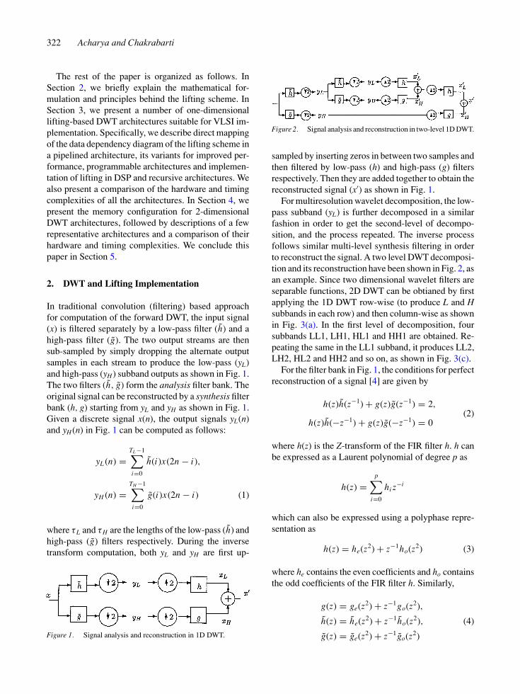
In traditional convolution (filtering) based approachfor computation of the forward DWT, the input signal(x) is filtered separately by a low-pass filter (h̃) and ahigh-pass filter (g̃). The two output streams are thensub-sampled by simply dropping the alternate outputsamples in each stream to produce the low-pass (yL)and high-pass (yH) subband outputs as shown in Fig. 1.The two filters (h̃, g̃) form the analysis filter bank. Theoriginal signal can be reconstructed by a synthesis filterbank (h, g) starting from yL and yH as shown in Fig. 1.Given a discrete signal x(n), the output signals yL(n)and yH(n) in Fig. 1 can be computed as follows:

yL (n) =TL−1∑

i=0

h̃(i)x(2n − i),

yH (n) =TH −1∑

i=0

g̃(i)x(2n − i) (1)

where τ L and τH are the lengths of the low-pass (h̃) andhigh-pass (g̃) filters respectively. During the inversetransform computation, both yL and yH are first up-

Figure 1. Signal analysis and reconstruction in 1D DWT.

Figure 2. Signal analysis and reconstruction in two-level 1D DWT.

sampled by inserting zeros in between two samples andthen filtered by low-pass (h) and high-pass (g) filtersrespectively. Then they are added together to obtain thereconstructed signal (x′) as shown in Fig. 1.

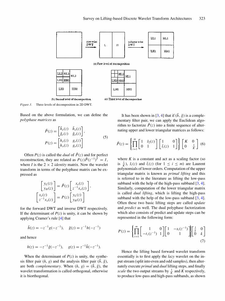
For multiresolution wavelet decomposition, the low-pass subband (yL) is further decomposed in a similarfashion in order to get the second-level of decompo-sition, and the process repeated. The inverse processfollows similar multi-level synthesis filtering in orderto reconstruct the signal. A two level DWT decomposi-tion and its reconstruction have been shown in Fig. 2, asan example. Since two dimensional wavelet filters areseparable functions, 2D DWT can be obtianed by firstapplying the 1D DWT row-wise (to produce L and Hsubbands in each row) and then column-wise as shownin Fig. 3(a). In the first level of decomposition, foursubbands LL1, LH1, HL1 and HH1 are obtained. Re-peating the same in the LL1 subband, it produces LL2,LH2, HL2 and HH2 and so on, as shown in Fig. 3(c).

For the filter bank in Fig. 1, the conditions for perfectreconstruction of a signal [4] are given by

h(z)h̃(z−1) + g(z)g̃(z−1) = 2,(2)

h(z)h̃(−z−1) + g(z)g̃(−z−1) = 0

where h(z) is the Z-transform of the FIR filter h. h canbe expressed as a Laurent polynomial of degree p as

h(z) =p∑

i=0

hi z−i

which can also be expressed using a polyphase repre-sentation as

h(z) = he(z2) + z−1ho(z2) (3)

where he contains the even coefficients and ho containsthe odd coefficients of the FIR filter h. Similarly,

g(z) = ge(z2) + z−1go(z2),

h̃(z) = h̃e(z2) + z−1h̃o(z2), (4)

g̃(z) = g̃e(z2) + z−1g̃o(z2)

Survey on Lifting-based Discrete Wavelet Transform Architectures 323

Figure 3. Three levels of decomposition in 2D DWT.

Based on the above formulation, we can define thepolyphase matrices as

P̃(z) =[

h̃e(z) h̃o(z)g̃e(z) g̃o(z)

],

(5)

P(z) =[

he(z) ge(z)ho(z) go(z)

]

Often P(z) is called the dual of P̃(z) and for perfectreconstruction, they are related as P(z)P̃(z−1)T = I ,where I is the 2 × 2 identity matrix. Now the wavelettransform in terms of the polyphase matrix can be ex-pressed as

[yL (z)yH (z)

]= P̃(z)

[xe(z)

z−1xo(z)

],

[xe(z)z−1xo(z)

]= P(z)

[yL (z)yH (z)

]

for the forward DWT and inverse DWT respectively.If the determinant of P(z) is unity, it can be shown byapplying Cramer’s rule [4] that

h̃(z) = −z−1g(−z−1), g̃(z) = z−1h(−z−1)

and hence

h(z) = −z−1g̃(−z−1), g(z) = z−1h̃(−z−1).

When the determinant of P(z) is unity, the synthe-sis filter pair (h, g) and the analysis filter pair (h̃, g̃),are both complementary. When (h, g) = (h̃, g̃), thewavelet transformation is called orthogonal, otherwiseit is biorthogonal.

It has been shown in [3, 4] that if (h̃, g̃) is a comple-mentary filter pair, we can apply the Euclidean algo-rithm to factorize P̃(z) into a finite sequence of alter-nating upper and lower triangular matrices as follows:

P̃(z) ={

m∏

i=1

[1 s̃2(z)0 1

] [1 0t̃i (z) 1

]} [K 00 1

K

](6)

where K is a constant and act as a scaling factor (sois 1

K ), s̃i (z) and t̃i (z) (for 1 ≤ i ≤ m) are Laurentpolynomials of lower orders. Computation of the uppertriangular matrix is known as primal lifting and thisis referred to in the literature as lifting the low-passsubband with the help of the high-pass subband [3, 4].Similarly, computation of the lower triangular matrixis called dual lifting, which is lifting the high-passsubband with the help of the low-pass subband [3, 4].Often these two basic lifting steps are called updateand predict as well. The dual polyphase factorizationwhich also consists of predict and update steps can berepresented in the following form:

P(z) ={

m∏

i=1

[1 0

−t i (z−1) 1

][1 −si (z−1)0 1

]}[1k 00 k

]

(7)

Hence the lifting based forward wavelet transformessentially is to first apply the lazy wavelet on the in-put stream (split into even and odd samples), then alter-nately execute primal and dual lifting steps, and finallyscale the two output streams by 1

K and K respectively,to produce low-pass and high-pass subbands, as shown


Figure 4. Lifting based forward and inverse DWT.

in Fig. 4(a). The inverse DWT can be derived bytraversing above steps in the reverse direction, firstscaling the low-pass and high-pass subband inputs byK and 1

K respectively, and then applying the dual andprimal lifting steps after reversing the signs of coef-ficients in t̃(z) and s̃(z) and finally the inverse lazytransform by up-scaling the output before mergingthem into a single reconstructed stream as shown inFig. 4(b).

Due to the linearity of the lifting scheme, if the inputdata is in integer format, it is possible to maintain datato be in integer format throughout the transform byintroducing a rounding function in the filtering opera-tion. Due to this property, the transform is reversible(i.e. lossless) and is called Integer Wavelet Transform(IWT) [5]. It should be noted that filter coefficientsneed not be integers for IWT. However, if a scaling stepis present in the factorization, IWT cannot be achieved.It has been proposed in [5] to split the scaling step intoadditional lifting steps to achieve IWT.

Example. Consider the (5, 3) filter that has been usedin JPEG2000 standard, with h̃ = (− 1

8 , 14 , 3

4 , 14 ,− 1

8 )and g̃ = (− 1

2 , 1,− 12 ).

h̃(z) = −1

8z−2 + 1

4z−1 + 3

4z0 + 1

4z − 1

8z2,

g̃(z) = −1

2z−2 + z−1 − 1

2z0

From above equations, we can easily derive that

h̃e(z2) = −1

8z−2 + 3

4− 1

8z2, h̃o(z2) = 1

4+ 1

4(z2),

g̃e(z2) = −1

2z−2 − 1

2, g̃o(z2) = 1.

As a result, polyphase matrix of this filter bank is

P̃(z) =[

h̃e(z) h̃o(z)g̃e(z) g̃o(z)

]

=[− 1

8 z−1 + 34 − 1

8 z 14 + 12

4 z− 1

2 z−1 − 12 1

]

Also based on conditions of perfect reconstructionsof the complementary filters as described in Eq. (2),we can derive the corresponding synthesis filters asfollows:

h(z) = −z−1g̃(−z−1) = 1

2z−1 + 1 + 1

2z,

g(z) = z−1h̃(−z−1)

= −1

8z−3 − 1

4z−2 + 3

4z−1 − 1

4− 1

8z.

Thus h = ( 12 , 1, 1

2 ) and g = (− 18 ,− 1

4 , 34 ,− 1

4 ,− 18 ).

Now based on the lifting scheme for factorization ofthe polyphase matrix, the possible factorization of P̃(z)that leads to a band matrix multiplication is

P̃(z) =[

1 14 (1 + z)

0 1

] [1 0

− 12 (1 + z−1) 1

]

If the samples are numbered starting from 0, we canconsider the even terms of the output stream as thesamples of lowpass subband and the odd terms as thesamples of highpass subband. Accordingly, we can in-terpret the above matrices in the time domain as y2i+1

= b(x2i + x2i+2) + x2i+1 and y2i = a(y2i+1 + y2i+3) +x2i, where 0 ≤ i ≤ N/2 for an input stream x and outputstream y both of length N, a = − 1

2 and b = 14 . Note

that the odd samples are calculated from even samplesand even samples are calculated from the updated oddsamples.

The other wavelet filter bank that has been proposedin JPEG2000 Part I standard is the (9,7) filter. The mostefficient factorization of the polyphase matrix for (9,7)filter is as follows [4]:

P̃(z) =[

1 a(1 + z−1)0 1

] [1 0

b(1 + z) 1

]

×[

1 c(1 + z−1)0 1

] [1 0

d(1 + z) 1

] [K 00 1

K

]

where a = −1.586134342, b = −0.05298011854,c = 0.8829110762, d = −0.4435068522, K =1.149604398.

In terms of banded matrix operation, the forwardtransform for (5,3) and (9,7) filters can be represented


as Y(5,3) = XM1M2 and Y(9,7) = XM1M2M3M4 re-spectively, while the corresponding inverse trans-form are represented as X = Y(5,3)M2M1 and X =Y(9,7)M4M3M2M1, where

M1 =

1 a 0 . . . . . .

0 1 0 0 . . . . .

0 a 1 a 0 . . . .

. 0 0 1 0 0 . . .

. . 0 a 1 a 0 . .

. . . 0 0 1 0 0 .

. . . . 0 a 1 a 0

. . . . . 0 0 1 0

0 . . . . . 0 a 1

,

M2 =

1 0 0 . . . . . .

0 1 b 0 . . . . .

0 0 1 0 0 . . . .

. 0 b 1 b 0 . . .

. . 0 0 1 0 0 . .

. . . 0 b 1 b 0 .

. . . . 0 0 1 0 0

. . . . . 0 b 1 0

0 . . . . . 0 0 1

M3 =

1 c 0 . . . . . .

0 1 0 0 . . . . .

0 c 1 c 0 . . . .

. 0 0 1 0 0 . . .

. . 0 c 1 c 0 . .

. . . 0 0 1 0 0 .

. . . . 0 c 1 c 0

. . . . . 0 0 1 0

0 . . . . . 0 c 1

,

M4 =

1 0 0 . . . . . .

0 1 d 0 . . . . .

0 0 1 0 0 . . . .

. 0 d 1 d 0 . . .

. . 0 0 0 1 0 . .

. . . 0 d 1 d 0 .

. . . . 0 0 1 0 0

. . . . . 0 d 1 0

0 . . . . . 0 0 1

In fact, most of the popular wavelet filters are de-composed either into 2 or 4 matrices (primal and dual).For example, the wavelet filters C(13, 7), S(13, 7), (2,6), (2, 10) can be decomposed into 2 matrices and (6,10) can be decomposed in 4 matrices as have beendescribed in detail in [12].

The lifting-based DWT has many advantages overthe convolution based approach. Some of them are asfollows.

• Lifting-based DWT typically requires less computa-tion (up to 50%) compared to the convolution basedapproach. However the savings depends upon thelength of the filters.

• During the lifting implementation, no extra memorybuffer is required because of the in-place computa-tion feature of lifting. This is particularly suitablefor hardware implementation with limited on-chipmemory.

• The lifting based approach offers integer to integertransformation suitable for lossless image compres-sion.

• In lossless transformation mode, the boundary ex-tension of the input data can be avoided becausethe original input can be exactly reconstructed byinteger to integer lifting transformation.

3. Lifting Architectures for 1D DWT

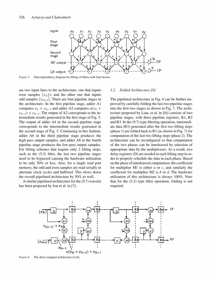
The data dependencies in the lifting scheme can beexplained with the help of an example of DWT filteringwith four factors (or four lifting steps). The four liftingsteps correspond to four stages as shown in Fig. 5. Theintermediate results generated in the first two stages forthe first two lifting steps are subsequently processed toproduce the high-pass (HP) outputs in the third stage,followed by the low-pass (LP) outputs in the fourthstage. (9,7) filter is an example of a filter that requiresfour lifting steps. For the DWT filters requiring onlytwo factors, such as the (5,3) filter, the intermediatetwo stages can simply be bypassed.

3.1. Direct Mapped Architecture [6]

A direct mapping of the data dependency diagram intoa pipelined architecture was proposed by Liu et al. in[6] and described in Fig. 6. The architecture is designedwith 8 adders (A1–A8), 4 multipliers (M1–M4), 6delay elements (D) and 8 pipeline registers (R). There


Figure 5. Data dependency diagram for lifting of filters with four factors.

are two input lines to the architecture: one that inputseven samples {x2i}), and the other one that inputsodd samples {x2i+1}. There are four pipeline stages inthe architecture. In the first pipeline stage, adder A1computes x2i + x2i−2 and adder A2 computes a(x2i +x2i−2) + x2i−1. The output of A2 corresponds to the in-termediate results generated in the first stage of Fig. 5.The output of adder A4 in the second pipeline stagecorresponds to the intermediate results generated inthe second stage of Fig. 5. Continuing in this fashion,adder A6 in the third pipeline stage produces thehigh-pass output samples, and adder A8 in the fourthpipeline stage produces the low-pass output samples.For lifting schemes that require only 2 lifting steps,such as the (5,3) filter, the last two pipeline stagesneed to be bypassed causing the hardware utilizationto be only 50% or less. Also, for a single read portmemory, the odd and even samples are read serially inalternate clock cycles and buffered. This slows downthe overall pipelined architecture by 50% as well.

A similar pipelined architecture for the (9,7) wavelethas been proposed by Jou et al. in [7].

3.2. Folded Architecture [8]

The pipelined architecture in Fig. 6 can be further im-proved by carefully folding the last two pipeline stagesinto the first two stages as shown in Fig. 7. The archi-tecture proposed by Lian, et al. in [8)] consists of twopipeline stages, with three pipeline registers, R1, R2and R3. In the (9,7) type filtering operation, intermedi-ate data (R3) generated after the first two lifting steps(phase 1) are folded back to R1 (as shown in Fig. 7) forcomputation of the last two lifting steps (phase 2). Thearchitecture can be reconfigured so that computationof the two phases can be interleaved by selection ofappropriate data by the multiplexors. As a result, twodelay registers (D) are needed in each lifting step in or-der to properly schedule the data in each phase. Basedon the phase of interleaved computation, the coefficientfor multiplier M1 is either a or c, and similarly thecoefficient for multiplier M2 is b or d. The hardwareutilization of this architecture is always 100%. Notethat for the (5,3) type filter operation, folding is notrequired.

Figure 6. The direct mapped architecture in [6].


Figure 7. The folded architecture in [8].

3.3. MAC Based Programmable Architecture [10]

A programmable architecture that implements the datadependencies represented in Fig. 5 using four MACs(Multiply and Accumulate) and nine registers has beenproposed by Chang et al. in [10]. The algorithm is ex-ecuted in two phases as shown in Fig. 8. The data-flowof the proposed architecture can be explained in termsof the register allocation of the nodes. The computationand allocation of the registers in phase 1 are done inthe following order

R0 ← x2i−1; R2 ← x2i ;R3 ← R0 + a(R1 + R2);R4 ← R1 + b(R5 + R3);R8 ← R5 + c(R6 + R4);OutputL P ← R6 + d(R7 + R8); OutputH P ← R8

Similarly, the computation and register allocation inphase 2 are done in the following order

R0 ← x2i+1; R1 ← x2i+2;R5 ← R0 + a(R2 + R1);

R6 ← R2 + b(R3 + R5);R7 ← R3 + c(R4 + R6);OutputL P ← R4 + d(R8 + R7); OutputH P ← R7

As a result, two samples are input per phase andtwo samples (LP and HP) are output at the end ofevery phase. For 2D DWT implementation, the outputsamples are also stored into a temporary buffer forfiltering in the vertical dimension.

3.4. Flipping Architecture [11]

While conventional lifting-based architectures requirefewer arithmetic operations, they sometimes have longcritical paths. For instance, the critical path of thelifting-based architecture for the (9,7) filter is 4Tm +8Ta while that of the convolution implementation isTm + 4Ta. One way of improving this is by pipeliningwhich results in a significant increase in the numberof registers. For instance, to pipeline the lifting-based

Figure 8. Data-flow and register allocation of the MAC based architecture in [10].


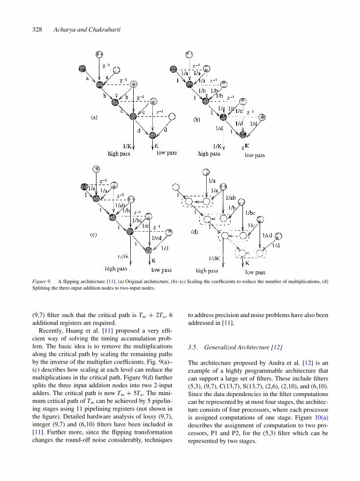
Figure 9. A flipping architecture [11]. (a) Original architecture, (b)–(c) Scaling the coefficients to reduce the number of multiplications, (d)Splitting the three-input addition nodes to two-input nodes.

(9,7) filter such that the critical path is Tm + 2Ta, 6additional registers are required.

Recently, Huang et al. [11] proposed a very effi-cient way of solving the timing accumulation prob-lem. The basic idea is to remove the multiplicationsalong the critical path by scaling the remaining pathsby the inverse of the multiplier coefficients. Fig. 9(a)–(c) describes how scaling at each level can reduce themultiplications in the critical path. Figure 9(d) furthersplits the three input addition nodes into two 2-inputadders. The critical path is now Tm + 5Ta. The mini-mum critical path of Tm can be achieved by 5 pipelin-ing stages using 11 pipelining registers (not shown inthe figure). Detailed hardware analysis of lossy (9,7),integer (9,7) and (6,10) filters have been included in[11]. Further more, since the flipping transformationchanges the round-off noise considerably, techniques

to address precision and noise problems have also beenaddressed in [11].

3.5. Generalized Architecture [12]

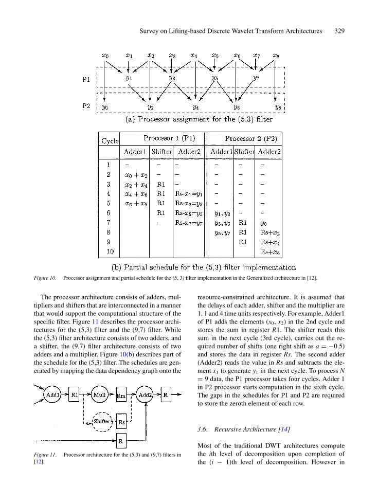
The architecture proposed by Andra et al. [12] is anexample of a highly programmable architecture thatcan support a large set of filters. These include filters(5,3), (9,7), C(13,7), S(13,7), (2,6), (2,10), and (6,10).Since the data dependencies in the filter computationscan be represented by at most four stages, the architec-ture consists of four processors, where each processoris assigned computations of one stage. Figure 10(a)describes the assignment of computation to two pro-cessors, P1 and P2, for the (5,3) filter which can berepresented by two stages.


Figure 10. Processor assignment and partial schedule for the (5, 3) filter implementation in the Generalized architecture in [12].

The processor architecture consists of adders, mul-tipliers and shifters that are interconnected in a mannerthat would support the computational structure of thespecific filter. Figure 11 describes the processor archi-tectures for the (5,3) filter and the (9,7) filter. Whilethe (5,3) filter architecture consists of two adders, anda shifter, the (9,7) filter architecture consists of twoadders and a multiplier. Figure 10(b) describes part ofthe schedule for the (5,3) filter. The schedules are gen-erated by mapping the data dependency graph onto the

Figure 11. Processor architecture for the (5,3) and (9,7) filters in[12].

resource-constrained architecture. It is assumed thatthe delays of each adder, shifter and the multiplier are1, 1 and 4 time units respectively. For example, Adder1of P1 adds the elements (x0, x2) in the 2nd cycle andstores the sum in register R1. The shifter reads thissum in the next cycle (3rd cycle), carries out the re-quired number of shifts (one right shift as a = −0.5)and stores the data in register Rs. The second adder(Adder2) reads the value in Rs and subtracts the ele-ment x1 to generate y1 in the next cycle. To process N= 9 data, the P1 processor takes four cycles. Adder 1in P2 processor starts computation in the sixth cycle.The gaps in the schedules for P1 and P2 are requiredto store the zeroth element of each row.

3.6. Recursive Architecture [14]

Most of the traditional DWT architectures computethe ith level of decomposition upon completion ofthe (i − 1)th level of decomposition. However in


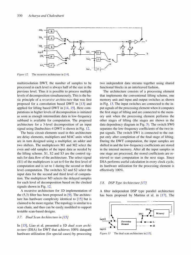
Figure 12. The recursive architecture in [14].

multiresolution DWT, the number of samples to beprocessed in each level is always half of the size in theprevious level. Thus it is possible to process multiplelevels of decomposition simultaneously. This is the ba-sic principle of a recursive architecture that was firstproposed for a convolution based DWT in [13] andapplied for lifting based DWT in [14, 15]. Here com-putations in higher levels of decomposition is initiatedas soon as enough intermediate data in low-frequencysubband is available for computation. The proposedarchitecture for a 3-level decomposition of an inputsignal using Daubechies-4 DWT is shown in Fig. 12.

The basic circuit elements used in this architectureare delay elements, multipliers and MAC units whichare in turn designed using a multiplier, an adder andtwo shifters. The multiplexors M1 and M2 select theeven and odd samples of the input data as needed bythe lifting scheme. S1, S2 and S3 are the control sig-nals for data flow of the architecture. The select signal(S1) of the multiplexors is set to 0 for the first level ofcomputation and is set to 1 during the second or thirdlevel computation. The switches S2 and S2 select theinput data for the second and third level of computa-tion. The multiplexor M3 selects the delayed samplesfor each level of decomposition based on the clockedsignals shown in Fig. 12.

A recursive architecture for 1D implementation ofthe (5,3) filter has been proposed in [9]. The architec-ture has hardware complexity identical to [15] but isclaimed to be more regular. The topology is similar to ascan chain, and thus can be easily modified to supporttestable scan-based designs.

3.7. Dual Scan Architecture in [15]

In [15], Liao et al. presented a 1D dual scan archi-tecture (DSA) for DWT that achieves 100% datapathhardware utilization (for special cases) by processing

two independent data streams together using sharedfunctional blocks in an interleaved fashion.

The architecture consists of a processing elementthat implements the conventional lifting scheme, onememory unit and input and output switches as shownin Fig. 13. The input switches are connected to the in-put signals of the processing element when it computesthe first stage of lifting and are connected to the mem-ory unit when the processing element performs theother stages of lifting (the stages are shown in thedata dependency diagram in Fig. 5). The switch SW0separates the low-frequency coefficients of the two in-put signals. The switch SW1 is connected to the out-put only after completion of the final stage of lifting.During the DWT computation, the input samples areshifted in and the low-frequency coefficients are storedin the internal memory. After all the input samples inone stage are processed, the stored coefficients are re-trieved to start computation in the next stage. SinceDSA performs useful calculation in every clock cycle,its hardware utilization for the processing element iseffectively 100%.

3.8. DSP Type Architecture [17]

A filter independent DSP type parallel architecturehas been proposed by Martina et al. in [17]. The

Figure 13 The dual scan architecture in [15].


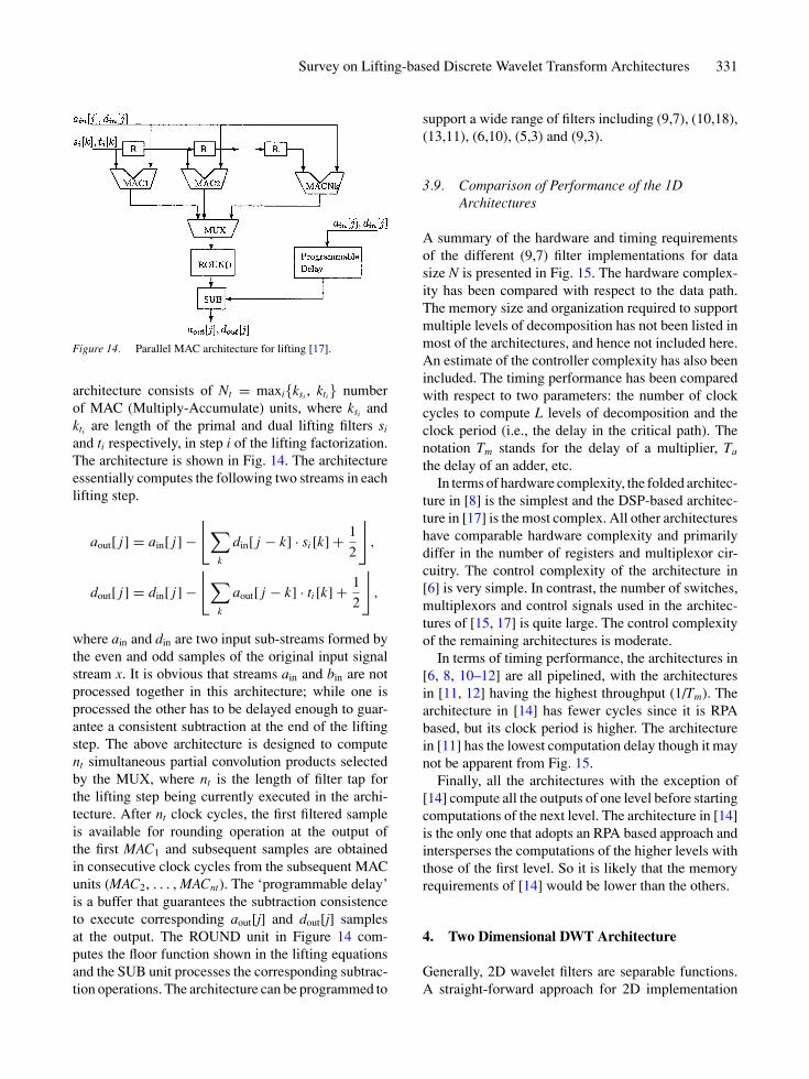
Figure 14. Parallel MAC architecture for lifting [17].

architecture consists of Nt = maxi{ksi , kti} numberof MAC (Multiply-Accumulate) units, where ksi andkti are length of the primal and dual lifting filters si

and ti respectively, in step i of the lifting factorization.The architecture is shown in Fig. 14. The architectureessentially computes the following two streams in eachlifting step.

aout[ j] = ain[ j] −⌊

∑

k

din[ j − k] · si [k] + 1

2

⌋,

dout[ j] = din[ j] −⌊

∑

k

aout[ j − k] · ti [k] + 1

2

⌋,

where ain and din are two input sub-streams formed bythe even and odd samples of the original input signalstream x. It is obvious that streams ain and bin are notprocessed together in this architecture; while one isprocessed the other has to be delayed enough to guar-antee a consistent subtraction at the end of the liftingstep. The above architecture is designed to computent simultaneous partial convolution products selectedby the MUX, where nt is the length of filter tap forthe lifting step being currently executed in the archi-tecture. After nt clock cycles, the first filtered sampleis available for rounding operation at the output ofthe first MAC1 and subsequent samples are obtainedin consecutive clock cycles from the subsequent MACunits (MAC2, . . . , MACnt). The ‘programmable delay’is a buffer that guarantees the subtraction consistenceto execute corresponding aout[j] and dout[j] samplesat the output. The ROUND unit in Figure 14 com-putes the floor function shown in the lifting equationsand the SUB unit processes the corresponding subtrac-tion operations. The architecture can be programmed to

support a wide range of filters including (9,7), (10,18),(13,11), (6,10), (5,3) and (9,3).

3.9. Comparison of Performance of the 1DArchitectures

A summary of the hardware and timing requirementsof the different (9,7) filter implementations for datasize N is presented in Fig. 15. The hardware complex-ity has been compared with respect to the data path.The memory size and organization required to supportmultiple levels of decomposition has not been listed inmost of the architectures, and hence not included here.An estimate of the controller complexity has also beenincluded. The timing performance has been comparedwith respect to two parameters: the number of clockcycles to compute L levels of decomposition and theclock period (i.e., the delay in the critical path). Thenotation Tm stands for the delay of a multiplier, Ta

the delay of an adder, etc.In terms of hardware complexity, the folded architec-

ture in [8] is the simplest and the DSP-based architec-ture in [17] is the most complex. All other architectureshave comparable hardware complexity and primarilydiffer in the number of registers and multiplexor cir-cuitry. The control complexity of the architecture in[6] is very simple. In contrast, the number of switches,multiplexors and control signals used in the architec-tures of [15, 17] is quite large. The control complexityof the remaining architectures is moderate.

In terms of timing performance, the architectures in[6, 8, 10–12] are all pipelined, with the architecturesin [11, 12] having the highest throughput (1/Tm). Thearchitecture in [14] has fewer cycles since it is RPAbased, but its clock period is higher. The architecturein [11] has the lowest computation delay though it maynot be apparent from Fig. 15.

Finally, all the architectures with the exception of[14] compute all the outputs of one level before startingcomputations of the next level. The architecture in [14]is the only one that adopts an RPA based approach andintersperses the computations of the higher levels withthose of the first level. So it is likely that the memoryrequirements of [14] would be lower than the others.

4. Two Dimensional DWT Architecture

Generally, 2D wavelet filters are separable functions.A straight-forward approach for 2D implementation


Figure 15. Hardware and timing comparison of the 1D DWT architectures for the (9, 7) filter computation on an input size N with L levels ofdecomposition.

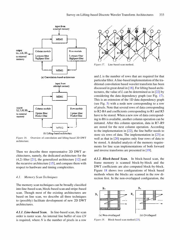
is to first apply the 1D DWT row-wise (to produceL and H subbands) and then column-wise to producefour subbands LL, LH, HL and HH as shown in Fig. 3in each level of decomposition. Obviously, the pro-cessor utilization is a concern in direct implementa-tion of this approach because it requires all the rowsbe filtered before the columnwise filtering can beginand thus it requires a size of memory buffer of theorder of the image size. The alternative approach isto begin the column-processing as soon as sufficientnumber of rows have been filtered. The column-wiseprocessing is now performed on these available lines toproduce wavelet coefficients row-wise. The overviewof the two-dimensional architecture for convolutionbased DWT is shown in Fig. 16(a). The row modulereads the data from MEM1, performs DWT along therows and writes the data into MEM2. The column mod-ule reads the data from MEM2, performs DWT alongthe columns and writes ‘LL’ data to MEM1 and ‘LH’,‘HL’, ‘HH’ data to external memory.

A similar approach can be implemented for the lift-ing scheme as well. The basic idea of lifting basedapproach for DWT implementation is to replace theparallel low-pass and high-pass filtering of traditional

approach by a sequence of alternating smaller filters.The computations in each filter can be partitioned intoprediction (dual lifting) and update (primal lifting)stages as shown in Fig. 16(b). Here the row modulereads the data from MEM1, performs the DWT alongthe rows (‘H’ and ‘L’) and writes the data into MEM2.The prediction filter of the column module reads thedata from MEM2, performs column-wise DWT alongalternate rows (‘HH’ and ‘LH’) and writes the datainto MEM2 in [12] (and into MEM1 in [21]); the up-date filter of the column module reads the data fromMEM2 in [12] (and MEM1 in [21]), performs column-wise DWT along the remaining rows, and writes the‘LL’ data into MEM1 for higher octave computationsand ‘HL’ data to external memory. Note that this is ageneric architectural flow and is the backbone of theexisting 2D architectures.

An important consideration in the design of 2D ar-chitectures is the memory configuration. A trade-offexists between the size of the internal memory and theframe memory access bandwidth. The size of the in-ternal memory is again a function of the way the framememory is scanned. In Section 4.1, we describe the ex-isting scanning techniques along the lines of [23, 22].


Figure 16. Overview of convolution and lifting-based 2D DWTarchitecture.

Then we describe three representative 2D DWT ar-chitectures, namely, the dedicated architecture for the(4,2) filter [21], the generalized architecture [12] andthe recursive architecture [15], and compare them withrespect to hardware and timing complexities.

4.1. Memory Scan Techniques

The memory scan techniques can be broadly classifiedinto line-based scan, block-based scan and stripe-basedscan. Though most of the existing architectures arebased on line scan, we describe all three techniquesto (possibly) facilitate development of new 2D DWTarchitectures.

4.1.1. Line-based Scan. In line-based scan, the scanorder is raster scan. An internal line buffer of size LNis required, where N is the number of pixels in a row

Figure 17. Line-based scan method.

and L is the number of rows that are required for thatparticular filter. A line-based implementation of the tra-ditional convolution based wavelet transform has beendiscussed in great detail in [18]. For lifting based archi-tectures, the value of L can be determined as in [22] byconsidering the data dependency graph (see Fig. 17).This is an extension of the 1D data dependency graph(see Fig. 5) with a node now corresponding to a rowof pixels. Note that several rows of data correspondingto R2-R4 and coefficients corresponding to R1 and R5have to be stored. When a new row of data correspond-ing to R6 is available, another column operation can beinitiated. After this column operation, data in R7–R9are stored for the next column operation. Accordingto the implementation in [22], the line buffer needs tostore six rows of data. The implementation in [23] aswell as that in [20] requires only four rows of data tobe stored. A detailed analysis of the memory require-ments for line scan implementations of both forwardand inverse transforms are presented in [19].

4.1.2. Block-based Scan. In block-based scan, theframe memory is scanned block-by-block and theDWT coefficients are also computed block-by-block.Figure 18 shows two configurations of block basedmethods where the blocks are scanned in the row di-rection first. In the non-overlapped configuration, the

Figure 18. Block-based scan method [23].


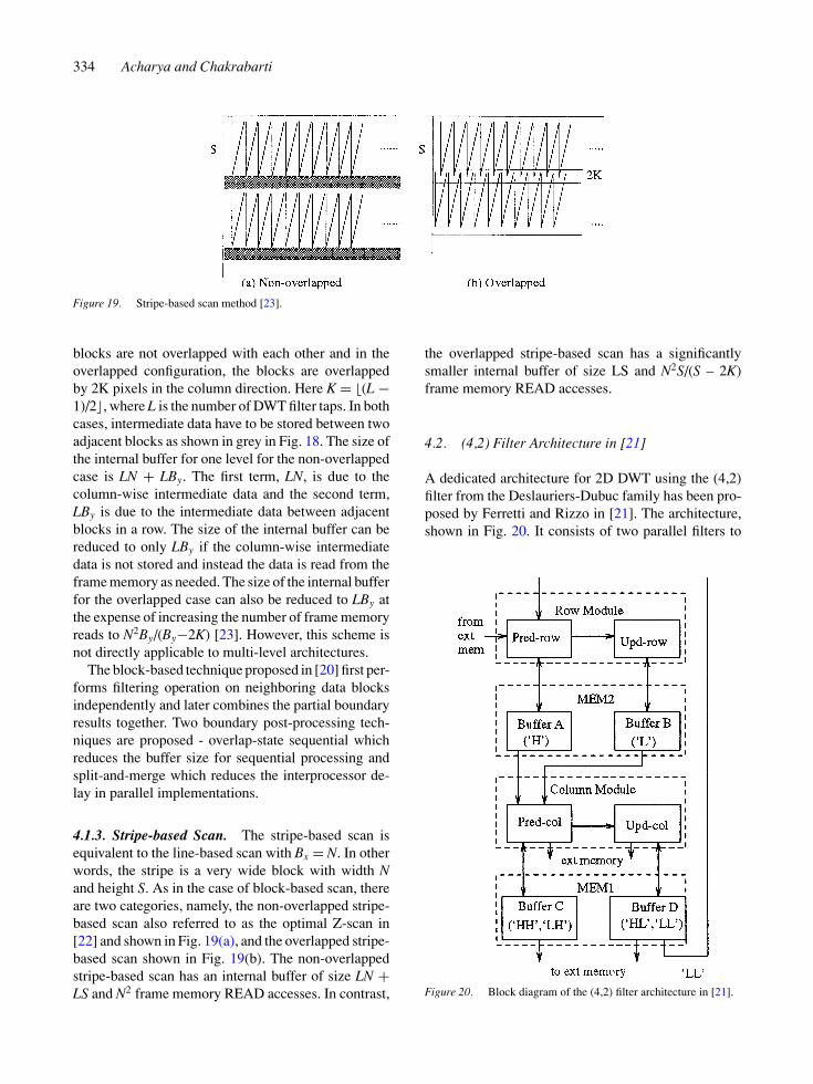
Figure 19. Stripe-based scan method [23].

blocks are not overlapped with each other and in theoverlapped configuration, the blocks are overlappedby 2K pixels in the column direction. Here K = �(L −1)/2�, where L is the number of DWT filter taps. In bothcases, intermediate data have to be stored between twoadjacent blocks as shown in grey in Fig. 18. The size ofthe internal buffer for one level for the non-overlappedcase is LN + LBy. The first term, LN, is due to thecolumn-wise intermediate data and the second term,LBy is due to the intermediate data between adjacentblocks in a row. The size of the internal buffer can bereduced to only LBy if the column-wise intermediatedata is not stored and instead the data is read from theframe memory as needed. The size of the internal bufferfor the overlapped case can also be reduced to LBy atthe expense of increasing the number of frame memoryreads to N2By/(By−2K) [23]. However, this scheme isnot directly applicable to multi-level architectures.

The block-based technique proposed in [20] first per-forms filtering operation on neighboring data blocksindependently and later combines the partial boundaryresults together. Two boundary post-processing tech-niques are proposed - overlap-state sequential whichreduces the buffer size for sequential processing andsplit-and-merge which reduces the interprocessor de-lay in parallel implementations.

4.1.3. Stripe-based Scan. The stripe-based scan isequivalent to the line-based scan with Bx = N. In otherwords, the stripe is a very wide block with width Nand height S. As in the case of block-based scan, thereare two categories, namely, the non-overlapped stripe-based scan also referred to as the optimal Z-scan in[22] and shown in Fig. 19(a), and the overlapped stripe-based scan shown in Fig. 19(b). The non-overlappedstripe-based scan has an internal buffer of size LN +LS and N2 frame memory READ accesses. In contrast,

the overlapped stripe-based scan has a significantlysmaller internal buffer of size LS and N2S/(S – 2K)frame memory READ accesses.

4.2. (4,2) Filter Architecture in [21]

A dedicated architecture for 2D DWT using the (4,2)filter from the Deslauriers-Dubuc family has been pro-posed by Ferretti and Rizzo in [21]. The architecture,shown in Fig. 20. It consists of two parallel filters to

Figure 20. Block diagram of the (4,2) filter architecture in [21].


compute the predict and update values along the rows(Pred-row, Upd-row), two parallel filters to computethe predict and update values along the columns (Pred-col, Upd-col), and four buffers A, B, C, D, to holdthe intermediate data to support the pipelined compu-tations. The buffers are dual-ported and are organizedsuch that 4 words can be accessed simultaneously. Eachfilter consists of multipliers (Lg = 4 for predict filtersand Lh = 2 for update filters), adders, shifters and in-ternal buffers (proportional to lg and Lh) to streamlinethe computations.

Pred-row computes on Lg = 4 data, Lg − 1 of whichare stored in its internal buffer. It computes the ‘H’values. The Upd-row requires Lh = 2 ‘H’ values tocompute a ‘L’ value. It obtains these by reading thelast value produced by Pred-row and storing the otherLh − 1 in internal registers. It picks up the primaryinput value from the internal buffer in Pred-row.

Pred-col performs the same basic operations asPred-row, though working on columns. It reads Lg

even position ‘H’ values along the columns. It pro-duces a new row of wavelet coefficients for every tworows produces by Pred-row. During the time Pred-rowproduces ‘H’ values for odd-indexed rows, Pred-colcomputes on the ‘L’ values generated by Upd-row.

The architecture utilization is only 50% if we onlyconsider the computations in the first level. The higherlevel computations can thus be easily interspersed withthe first level computations using a RPA-based ap-proach. In fact, once the unit delay for any level isdetermined, the schedule can be easily obtained. Pleaserefer to [21] for details of the schedules, memory sizes,number of read/write accesses, etc.

4.3. Generalized 2D DWT Architecture in [12]

The architecture proposed by Andra et al. [12] is moregeneralized and can compute a large set of filters forboth the 2D forward and inverse transforms. It sup-ports two classes of architectures based on whetherlifting is implemented by one or two lifting steps. TheM2 architecture corresponds to implementation usingone lifting step or two factorization matrices, and theM4 architecture corresponds to implementation by twolifting steps or four factorization matrices.

The dataflow of the M2 architecture that is used toimplement the wavelet filters (5,3), C(13,7), S(13,7),(2,6), (2,10) is similar to that in Fig. 16(b). A blockdiagram of the M2 architecture is shown in Fig. 21.

Figure 21. Block diagram of the generalized M2 architecture in[12].

It consists of the row and column computation mod-ules and two memory units, MEM1 and MEM2. Therow module consists of two processors RP1 and RP2along with a register file REG1, and the column mod-ule consists of two processors CP1 and CP2 along witha register file REG2. All the four processors RP1, RP2,CP1, CP2 in the proposed architecture consists of 2adders, 1 multiplier and 1 shifter as shown in Fig. 11.

Figure 22. Data access patterns for the row and column modulesfor the (5,3) filter with N = 5 in the 2D DWT architecture in [12].


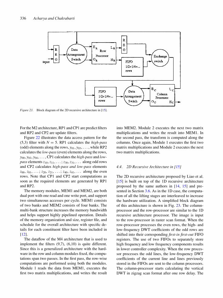
Figure 23. Block diagram of the 2D recursive architecture in [15].

For the M2 architecture, RP1 and CP1 are predict filtersand RP2 and CP2 are update filters.

Figure 22 illustrates the data access pattern for the(5,3) filter with N = 5. RP1 calculates the high-pass(odd) elements along the rows, y01, y03, . . . , while RP2calculates the low-pass (even) elements along the rows,y00, y02, y04, . . . , CP1 calculates the high-pass and low-pass elements z10, z11, . . . ; z30, z31, . . . along odd rowsand CP2 calculates high-pass and low-pass elementsz00, z01, . . . ; z20, z21, . . . ; z40, z41, . . . along the evenrows. Note that CP1 and CP2 start computations assoon as the required elements are generated by RP1and RP2.

The memory modules, MEM1 and MEM2, are bothdual port with one read and one write port, and supporttwo simultaneous accesses per cycle. MEM1 consistsof two banks and MEM2 consists of four banks. Themulti-bank structure increases the memory bandwidthand helps support highly pipelined operation. Detailsof the memory organization and size, register file, andschedule for the overall architecture with specific de-tails for each constituent filter have been included in[12].

The dataflow of the M4 architecture that is used toimplement the filters (9,7), (6,10) is quite different.Since this is a generalized architecture with the hard-ware in the row and column modules fixed, the compu-tations span two passes. In the first pass, the row-wisecomputations are performed using both the modules.Module 1 reads the data from MEM1, executes thefirst two matrix multiplications, and writes the result

into MEM2. Module 2 executes the next two matrixmultiplications and writes the result into MEM1. Inthe second pass, the transform is computed along thecolumns. Once again, Module 1 executes the first twomatrix multiplications and Module 2 executes the nexttwo matrix multiplications.

4.4. 2D Recursive Architecture in [15]

The 2D recursive architecture proposed by Liao et al.[15] is built on top of the 1D recursive architectureproposed by the same authors in [14, 15] and pre-sented in Section 3.6. As in the 1D case, the computa-tion of all the lifting stages are interleaved to increasethe hardware utilization. A simplified block diagramof this architecture is shown in Fig. 23. The column-processor and the row-processor are similar to the 1Drecursive architecture processor. The image is inputto the row-processor in raster scan format. When therow-processor processes the even rows, the high- andlow-frequency DWT coefficients of the odd rows areshifted into their corresponding first-in first-out FIFOregisters. The use of two FIFOs to separately storehigh frequency and low frequency components resultsin lower controller complexity. When the row proces-sor processes the odd lines, the low-frequency DWTcoefficients of the current line and lines previouslystored in the FIFOs are sent to the column processors.The column-processor starts calculating the verticalDWT in zigzag scan format after one row delay. The


Figure 24. Hardware and timing comparison of the 2D DWT Architectures on an input of size N × N with L levels of decomposition.

computations are arranged in a way that the DWT co-efficients of the first stage are interleaved with the otherstages. The arrangement is done with the help of thedata arrangement switches at the input to the row andcolumn processors, and the exchange switch.

A mix of the principles of recursive pyramid al-gorithm (RPA) [13] and folded architecture has beenadopted by Jung et al. to design a 2D architecturefor lifting based DWT in [16]. The row-processor isa 1D folded architecture and does row-wise compu-tations in the usual fashion. The column processoris responsible for filtering along the columns at thefirst level and filtering along both the rows and thecolumns at the higher levels. It does this by employ-ing RPA scheduling and achieves very high utiliza-tion. The utilization of the row processor is 100%,and that of the column processor is 83% for 5-leveldecomposition.

4.5. Other 2D DWT Architectures

Several of the 1D DWT architectures proposed in Sec-tion 3 can be extended to compute 2D DWT usingthe row-column method. If a frame memory based ap-proach is used where the original samples are replacedby the calculated coefficients, no additional memoryis required. However, an address generator is neededto provide the proper access addresses in order to readsamples for the next level computation and then writethem back as in [8]. If a frame memory is not allowed,then most architectures implement some form of theline scan method. The architecture in [8] uses an in-

ternal buffer of size BN, where B is the height of thecode block in a JPEG2000 architecture. The line-basedimplementation in [10] organizes the line buffer intotwo parts: the signal memory which stores both thelow pass and the high pass outputs corresponding tothe row-wise computations and the temporary memorywhich stores the temporary results for the column-wisecomputations. Details of the size of the memory as wellas nature of memory accesses are described. A genericline-based implementation of an RPA-based approachhas been presented in [24]. The important feature hereis the efficient use of 2-port RAMs to implement theline buffers.

The 2D extension of the dual scan architecture(DSA) (see Section 3.7 for the 1D DSA) is also aline based implementation. Here two consecutiverows are scanned simultaneously in line scan orderand the column processor computes on the row DWTcoefficients. The row-processor in 2D DSA is identicalto the 1D DSA presented in Section 3.7; registers areused to hold the even and odd pixels of each row and tointerleave the input pairs of two consecutive rows. Theinternals of the column processor is the same as the rowprocessor. However the 1 pixel registers in the row pro-cessors are replaced by 1-row delay units. Comparedto conventional architectures, DSA needs roughly halfof the time to compute lifting based 2-D DWT.

4.6. Comparison of Performances

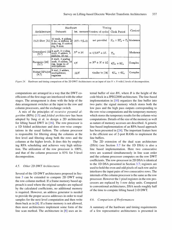
A summary of the hardware and timing requirementsof a few representative architectures is presented in


Fig. 24. The hardware complexity has been describedin terms of datapath components and internal memorysize. We list only the internal memory size since all thearchitectures require an external memory of size N2

for input data of size N × N. The timing performancehas been compared with respect to the number of clockcycles to compute L levels of decomposition and theclock period.

Of the four architectures, the architecture in [15] hasthe smallest internal memory. This is because [15] is anRPA based approach that intersperses the computationsat the higher levels with those of the lower levels. Thearchitecture in [12], on the other hand, computes all theoutputs of one level before starting the computationsat the next level and has an internal memory of sizeO(N2). The datapath complexity of the architecture in[12] is by far the lowest.

The control complexity of the architecture in [15] issignificantly higher than the others. This is because ofthe large number of control signals and switches thatare used to organize the data before sending to the rowand column computation units.

In terms of the timing performance, the architecturein [12] is pipelined and has the highest throughput(1/Tm). The architecture in [15, 16] requires the fewestnumber of cycles since they are RPA based, though theclock periods are significantly higher.

The architecture in [21] is specific to the (4,2) filterswhile the RPA concept that is applied to the architec-tures in [15, 16] can be applied to a large set of filters(not just (3,5), (9,7), Daub-4). The architecture in [12]is essentially a programmable architecture which sup-ports implementation of a large set of filters on thesame hardware platform.

5. Conclusions

In this paper, we presented a survey of the existinglifting based implementations of 1-dimensional and 2-dimensional Discrete Wavelet Transform. We brieflydescribed the principles behind the lifting scheme inorder to better understand the different implementationstyles and structures. We have presented several archi-tectures of different flavors ranging from highly paral-lel ones to highly folded ones to programmable ones.We provided a systematic derivation of each architec-ture and evaluated them with respect to their hardwareand timing requirements.

References

1. S. Mallat, “A Theory for Multiresolution Signal Decomposition:The Wavelet Representation,” IEEE Trans. Pattern Analysis AndMachine Intelligence, vol. 11, no. 7, 1989, pp. 674–693.

2. T. Acharya and P. S. Tsai, JPEG2000 Standard for Image Com-pression: Concepts, Algorithms and VLSI Architectures. JohnWiley & Sons, Hoboken, New Jersey, 2004.

3. W. Sweldens, “The Lifting Scheme: A Custom-Design Con-struction of Biorthogonal Wavelets,” Applied and Computa-tional Harmonic Analysis, vol. 3, no. 15, 1996, pp. 186–200.

4. I. Daubechies and W. Sweldens, “Factoring Wavelet Transformsinto Lifting Schemes,” The J. of Fourier Analysis and Applica-tions, vol. 4, 1998, pp. 247–269.

5. M.D. Adams and F. Kossentini, “Reversible Integer-to-IntegerWavelet Transforms for Image Compression: Performance Eval-uation and Analysis,” IEEE Trans. on Image Processing, vol. 9,2000, pp. 1010–1024.

6. C.C. Liu, Y.H. Shiau, and J.M. Jou, “Design and Implementationof a Progressive Image Coding Chip Based on the Lifted WaveletTransform,” in Proc. of the 11th VLSI Design/CAD Symposium,Taiwan, 2000.

7. J.M. Jou, Y.H. Shiau, and C.C. Liu, “Efficient VLSI Architec-tures for the Biorthogonal Wavelet Transform by Filter Bank andLifting Scheme,” in IEEE International Symposium on Circuitsand Systems, Sydney, Australia, 2001, pp. 529–533.

8. C.J Lian, K.F. Chen, H.H. Chen, and L.G. Chen, “Lifting BasedDiscrete Wavelet Transform Architecture for JPEG2000,” inIEEE International Symposium on Circuits and Systems, Syd-ney, Australia, 2001, pp. 445–448.

9. P.-Y. Chen, “VLSI Implementation for One-Dimensional Multi-level Lifting-Based Wavelet Transform,” IEEE Transactions onComputers, vol. 53, no. 4, 2004.

10. W.H. Chang, Y.S. Lee, W.S. Peng, and C.Y. Lee, “A Line-Based,Memory Efficient and Programmable Architecture for 2D DWTUsing Lifting Scheme,” in IEEE International Symposium onCircuits and Systems, Sydney, Australia, 2001, pp. 330–333.

11. C.T. Huang, P.C. Tseng, and L.G. Chen, “Flipping Structure: AnEfficient VLSI Architecture for Lifting-Based Discrete WaveletTransform,” in IEEE Transactions on Signal Processing, 2004,pp. 1080–1089.

12. K. Andra, C. Chakrabarti, and T. Acharya, “A VLSI Architec-ture for Lifting-Based Forward and Inverse Wavelet Transform,”IEEE Trans. of Signal Processing, vol. 50, no. 4, 2002, pp. 966–977.

13. M. Vishwanath, “The Recursive Pyramid Algorithm for the Dis-crete Wavelet Transform,” in IEEE Transactions on Signal Pro-cessing, vol. 42, 1994, pp. 673–676.

14. H. Liao, M.K. Mandal, and B.F. Cockburn, “NovelArchitectures for Lifting-Based Discrete Wavelet Trans-form,” in Electronics Letters, vol. 38, no. 18, 2002,pp. 1010–1012.

15. H. Liao, M.K. Mandal, and B.F. Cockburn, “Efficient Architec-tures for 1-D and 2-D Lifting-Based Wavelet Transform,” IEEETransactions on Signal Processing, vol. 52, no. 5, 2004, pp.1315–1326.

16. G.C. Jung, D.Y. Jin, and S.M. Park, “An Efficient Line BasedVLSI Architecture for 2-D Lifting DWT,” in The 47th IEEE In-ternational Midwest Symposium on Circuits and Systems, 2004.


17. M. Martina, G. Masera, G. Piccinini, and M. Zamboni, “NovelJPEG 2000 Compliant DWT and IWT VLSI Implementations,”Journal of VLSI Signal Processing, vol. 34, 2003, pp. 137–153.

18. C. Chrysafis and A. Ortega, “Line-Based, Reduced Memory,Wavelet Image Compression,” IEEE Trans. on Image Process-ing, vol. 9, no. 3, 2000, pp. 378–389.

19. J. Reichel, M. Nadenau, and M. Kunt, “Row-Based WaveletDecomposition Using the Lifting Scheme,” Proceedings of theWorkshop on Wavelet Transforms and Filter Banks, Branden-burg an der Havel, Germany, March 5–7, 1999.

20. W. Jiang and A. Ortega, “Lifting Factorization-Based DiscreteWavelet Transform Architecture Design,” IEEE Trans, on Cir-cuits and Systems for Video Technology, vol. 11, 2001, pp. 651–657.

21. M. Ferretti and D. Rizzo, “A Parallel Architecture for the 2-D Discrete Wavelet Transform with Integer Lifting Scheme,”Journal of VLSI Signal Processing, vol. 28, 2001, pp. 165–185.

22. M.Y. Chiu, K.-B. Lee, and C.-W. Jen, “Optimal Data Transferand Buffering Schemes for JPEG 20000 Encoder,” in Proceed-ings of the IEEE Workshop on Design and Implementation ofSignal Processing Systems, 2003, pp. 177–182.

23. C.-T. Huang, P.-C. Tseng, and L.-G. Chen, “Memory Anal-ysis and Architecture for Two-Dimensional Discrete WaveletTransform,” in Proceedings of the IEEE Int. Conf. onAcoustics, Speech and Signal Processing, 2004, pp. V13–V16.

24. P.-C. Tseng, C.-T. Huang, and L.-G. Chen, “Generic RAM-Based Architecture for Two-Dimensional Discrete WaveletTransform with Line-Based Method,” in Proceedings of theAsia-Pacific Conference on Circuits and Systems, 2002, pp. 363–366.

Tinku Acharya received his B.Sc. (Honors) in Physics, B.Tech. andM.Tech. in Computer Science from University of Calcutta, India, andthe Ph.D. in Computer Science from University of Central Florida,USA, in 1984, 1987, 1989, and 1994, respectively. He is currently theChief Technology Officer of Avisere Inc., Tucson, Arizona, USA.Dr. Acharya is also an Adjunct Professor in the Department of Elec-trical Engineering, Arizona State University, Tempe, USA.

Before joining Avisere, Dr. Acharya served in Intel Corporation(1996–2002), where he led several R&D teams toward develop-ment of algorithms and architectures in image and video processing,multimedia computing, PC-based digital camera, reprographics ar-chitecture for color photo-copiers, 3G cellular telephony, analysisof next-generation microprocessor architecture, etc. Before Intel,

Dr. Acharya was a consulting engineer at AT&T Bell Laboratories(1995–1996), a research faculty at the Institute of Systems Research,Institute of Advanced Computer Studies, University of Maryland atCollege Park (1994–1995), and held visiting faculty positions atIndian Institute of Technology, Kharagpur. He served as SystemsAnalyst in National Informatics Center, Planning Commission, Gov-ernment of India (1988–1990). He collaborated in research and de-velopment with Xerox Palo Alto Research Center (PARC), EastmanKodak Corporation, and many other institutions worldwide.

Dr. Acharya is inventor of 88 US patents and 14 European patents.He authored over 80 technical papers and four books—Image Pro-cessing: Principles and Applications (Wiley, New Jersey, 2005),JPEG2000 Standard for Image Compression: Concepts, Algorithms,and VLSI Architectures (Wiley, 2004), Information Technology:Principles and Applications (Prentice-Hall India, 2004), and DataMining: Multimedia, Soft Computing and Bioinformatics (Wiley,2003).

Dr. Acharya is a Fellow of the National Academy of Engineers(India), Life Fellow of the Institution of Electronics and Telecom-munication Engineers (FIETE), and Senior Member of IEEE. Hiscurrent research interests are in computer vision, image processing,multimedia data mining, bioinformatics, and VLSI architectures andalgorithms.tinku [email protected]

Chaitali Chakrabarti received the B.Tech. degree in electronicsand electrical communication engineering from the Indian Instituteof Technology, Kharagpur, India in 1984, and the M.S. and Ph.Ddegrees in electrical engineering from the University of Marylandat College Park, USA, in 1986 and 1990 respectively. Since August1990, she has been with the Department of Electrical Engineering,Arizona State University, Tempe, where she is now a Professor.Her research interests are in the areas of low power embedded sys-tems design including memory optimization, high level synthesisand compilation, and VLSI architectures and algorithms for signalprocessing, image processing and communications.

Dr. Chakrabarti is a member of the Center for Low Power Elec-tronics, the Consortium for Embedded Systems and Connection One.She received the Research Initiation Award from the National Sci-ence Foundation in 1993, a Best Teacher Award from the College ofEngineering and Applied Sciences, ASU, in 1994, and the Outstand-ing Educator Award from the IEEE Phoenix section in 2001. Shehas served on the program committees of ICASSP, ISCAS, SIPS,ISLPED and DAC. She is currently an Associate Editor of the IEEETransactions on Signal Processing and the Journal of VLSI SignalProcessing Systems. She is also the TC Chair of the sub-committeeon Design and Implementation of Signal Processing Systems, IEEESignal Processing [email protected]