Parallel Computing 59 (2016) 43–59

Contents lists available at ScienceDirect

Parallel Computing

journal homepage: www.elsevier.com/locate/parco

A parallel min-cut algorithm using iteratively reweighted least

squares targeting at problems with floating-point edge

weights

Yao Zhu

∗, David F. Gleich

Department of Computer Science, Purdue University, 305 N. University Street, West Lafayette, IN 47907, USA

a r t i c l e i n f o

Article history:

Received 30 March 2015

Revised 21 November 2015

Accepted 22 February 2016

Available online 3 March 2016

Keywords:

Undirected graphs

s –t min-cut

Iteratively reweighted least squares

Laplacian systems

Parallel linear system solvers

a b s t r a c t

We present a parallel algorithm for the undirected s –t min-cut problem with floating-

point valued edge weights. Our overarching algorithm uses an iteratively reweighted least

squares framework. Specifically, this algorithm generates a sequence of Laplacian linear

systems, which are solved in parallel. The iterative nature of our algorithm enables us

to trade off solution quality for execution time, which is distinguished from those purely

combinatorial algorithms that only produce solutions at optimum. We also propose a novel

two-level rounding procedure that helps to enhance the quality of the approximate min-

cut solution output by our algorithm. Our overall implementation, including the round-

ing procedure, demonstrates significant speed improvement over a state-of-the-art serial

solver, where it could be up to 200 times faster on commodity platforms.

© 2016 Elsevier B.V. All rights reserved.

1. Introduction

We consider the undirected s –t min-cut problem. Our goal is a practical, scalable, parallel algorithm for problems with

hundreds of millions or billions of edges and with floating point weights on the edges. Additionally, we expect there to be

a sequence of such s –t min-cut computations where the difference between successive problems is small. The motivation

for such problems arises from a few recent applications including the FlowImprove method to improve a graph partition [1]

and the GraphCut method to segment high-resolution images and MRI scans [2,3] . Both of these applications are limited by

the speed of current s –t min-cut solvers, and the fact that most of them cannot handle problems with floating point edge

weights. We seek to accelerate such s –t min-cut computations, especially on floating point valued instances.

For the undirected s –t min-cut problem, we present a Parallel Iteratively Reweighted least squares Min-Cut solver, which

we call PIRMCut for convenience. This algorithm draws its inspiration from the recent theoretical work on using Laplacians

and electrical flows to solve max-flow/min-cut in undirected graphs [4–6] . However, our exposition and derivation is entirely

self-contained. In contrast to traditional combinatorial solvers for this problem, our method produces an approximate min-

cut solution, just like many of the recent theory papers [4–6] .

There are three essential ingredients to our approach. The first essential ingredient is a variational representation of the

� 1 -minimization formulation of the undirected s –t min-cut ( Section 2.1 ). This representation allows us to use the iteratively

reweighted least squares (IRLS) method to generate a sequence of symmetric diagonally dominant linear systems whose

∗ Corresponding author. Tel.: +1 7654305239.

E-mail addresses: yaozhu@purdue.edu (Y. Zhu), dgleich@purdue.edu (D.F. Gleich).

http://dx.doi.org/10.1016/j.parco.2016.02.003

0167-8191/© 2016 Elsevier B.V. All rights reserved.

44 Y. Zhu, D.F. Gleich / Parallel Computing 59 (2016) 43–59

solutions converge to an approximate solution ( Theorem 2.6 ). We show that these systems are equivalent to electrical flows

computation ( Proposition 2.3 ). We also prove a Cheeger-type inequality that relates an undirected s –t min-cut to a general-

ized eigenvalue problem ( Theorem 2.7 ). The second essential ingredient is a parallel implementation of the IRLS algorithm

using a parallel linear system solver. The third essential ingredient is a two-level rounding procedure that uses information

from the electrical flow solution to generate a much smaller s –t min-cut problem suitable for serial s –t min-cut solvers.

The current state-of-the-art combinatorial s –t max-flow/min-cut solvers [7–10] are all based on operating the residual

graph. The residual graph and associated algorithms are usually associated with complex data structures and updating pro-

cedures. Thus, the operations on it would result in irregular memory access patterns. Moreover, the directed edges of the

residual graph come and go frequently during algorithm execution. This dynamically changing structure of the residual

graph further exacerbates the irregularity of the s –t min-cut computation if the combinatorial solvers are used. In contrast,

PIRMCut reduces the s –t min-cut problem to solving a sequence of Laplacian systems all with the same fixed nonzero struc-

ture. Because then only matrix computations are used, such a reduction also gets rid of the need for complex updating

procedures. Although it does not necessarily wipe out the irregularity of the application, it does significantly diminishes

the degree of irregularity. In fact, it has been demonstrated that irregular applications rich in parallel sparse matrix com-

putations can obtain significant speedups on multithreaded platforms [11] . In a broader sense, the algorithmic paradigm

embodied by PIRMCut, i.e., reducing irregular graph applications to more regular matrix computations, could facilitate the

adoption of modern high performance computing systems and architectures, especially those specifically designed for irreg-

ular applications [12–14] .

We have designed and implemented an MPI based implementation of PIRMCut and evaluated its performance on both

distributed and shared memory machines using a set of test problems consisting of different kinds of graphs. Our solver,

PIRMCut, is 200 times faster (using 32 cores) than a state-of-the-art serial s –t min-cut solver on a test graph with no

essential difference in quality. In the experimental results, we also demonstrate the benefit of using warm starts when

solving a sequence of related linear systems. We further show the advantage of the proposed two-level rounding procedure

over the standard sweep cut in producing better approximate solutions.

At the moment, we do not have a precise and graph-size based runtime bound on PIRMCut. We also acknowledge that,

like most numerical solvers, it is only up to δ-accurate. The focus of this paper is investigating and documenting a set of

techniques that are principled and could lead to practically fast solutions on real world s –t min-cut problems. We com-

pare our approach with those of others and discuss some further opportunities of our approach in the related work and

discussions ( Sections 4 and 6 ).

2. An IRLS algorithm for undirected s –t min-cut

In this section, we describe the derivation of the IRLS algorithm for the undirected s –t min-cut problem. We first in-

troduce our notations. Let G = (V, E ) be a weighted, undirected graph. In the derivation that follows, the term weight will

be reserved to denote the set of weights that result from the IRLS algorithm. Thus, at this point, we wish to refer to the

edge weights as capacities following the terminology in network flow problems. Let n = |V| , and m = |E| . We require for each

undirected edge { u, v } ∈ E, its capacity c({ u, v } ) > 0 . Let s and t be two distinguished nodes in G, and we call s the source

node and t the sink node . The problem of undirected s –t min-cut is to find a partition of V = S ∪ S̄ with s ∈ S and t ∈ S̄ such

that the cut value

cut (S, S̄ ) =

∑

{ u, v }∈E u ∈S, v ∈ ̄S

c({ u, v } )

is minimized. In the interest of solving the undirected s –t min-cut problem, we assume G to be connected. We call the

subgraph of G induced on V\{ s, t} the non-terminal graph , and denote it by ˜ G = ( ̃ V , ̃ E ) . We call the edges incident to s or t

the terminal edges , and denote them by E T . The undirected s –t min-cut problem can be formulated as an � 1 -minimization problem. Let B ∈ {−1 , 0 , 1 } m ×n be the

edge-node incidence matrix corresponding to an arbitrary orientation of G’s edges, and C be the m × m diagonal matrix

with c({ u, v } ) on the main diagonal. Further let f = [1 0] T , and �

T = [ e s e t ] where e s ( e t ) is the s th ( t th) standard basis,

then the undirected s –t min-cut problem is

minimize x

|| CBx || 1 subject to �x = f , x ∈ [0 , 1] n .

(1)

Note that in (1) we adopt the constraint x ∈ [0, 1] n instead of the integral constraint x ∈ {0, 1} n . This change is justified

because once the st min-cut problem is converted into a linear program in standard form, the matrix B appears in the

constraints. The incidence matrix B is a standard example of totally unimodular [15] . Thus, such a relaxation does not

change the set of integral optimal solutions.

Y. Zhu, D.F. Gleich / Parallel Computing 59 (2016) 43–59 45

˜

2.1. The IRLS algorithm

The IRLS algorithm for solving the � 1 -minimization problem (1) is motivated by the variational representation of the � 1norm

‖ z ‖ 1 = min w ≥0 1 2

∑

i

(z 2

i

w i + w i

).

Using this variational representation, we can rewrite the � 1 -minimization problem (1) as the following joint minimization

problem:

minimize x , w ≥0

H(x , w ) =

1

2

∑

i

((CBx ) 2

i

w i

+ w i

)(2)

subject to �x = f , x ∈ [0 , 1] n (3)

The IRLS algorithm for (1) can be derived by applying alternating minimization to (2) [16] . Given an IRLS iterate x (l−1)

satisfying constraint (3) , the next IRLS iterate x ( l ) is defined according to the following two alternating steps:

• Step 1: Compute the reweighting vector w

( l ) , of which each component is defined by

w

(l) i

=

√

(CBx

(l−1) ) 2 i

+ ε2 (4)

where ε > 0 is a smoothing parameter that guards against the case of (CBx (l−1) ) i = 0 . • Step 2: Let W

(l) = diag (w

(l) ) , update x ( l ) by solving the weighted least squares (WLS) problem

minimize x

1

2

x

T

B

T

C (W

(l) ) −1 CBx subject to �x = f . (5)

We prove that the sequence of iterates from the IRLS algorithm is well-defined, that is, each iterate x ( l ) exists and satisfies

x ( l ) ∈ [0, 1] n . Solving (5) leads to solving the saddle point problem [L (l) �

T

� O

][x

λ

]=

[0

f

](6)

where λ is the Lagrange multiplier corresponding to the constraint �x = f , and L ( l ) is defined as follows:

L (l) = B

T

C (W

(l) ) −1 CB (7)

We note that L ( l ) is a reweighted Laplacian of G, where the edge capacities C are reweighted by the diagonal matrix

(W

(l) ) −1 . For a recent survey on graph Laplacians, we refer to [17] . Regarding the nonsingularity of the linear system (6) ,

we have the following proposition.

Proposition 2.1. A sufficient and necessary condition for the linear system (6) to be nonsingular is that G is connected.

Proof. When G is connected, ker (L (l) ) = span { e } , where e is the all-one vector. From the definition of �, we know e �∈ker (�) , i.e., ker (L (l) ) ∩ ker (�) = { 0 } . With � being full rank, we apply Theorem 3.2 from [18] to prove the proposition. �

We now prove that the solution x ( l ) to (6) automatically satisfies the interval constraint.

Proposition 2.2. If G is connected, then for each IRLS update we have x ( l ) ∈ [0, 1] n .

Proof. According to proposition 2.1 , the linear system (6) is nonsingular when G is connected. We apply the null space

method [18] to solve it. Let Z be the matrix from deleting the s , t columns of the identity matrix I n , then Z is a null basis

of �. Because �e s = f , using Z and e s we reduce (6) to the following linear system:

(Z

T

L (l) Z ) v = −Z

T

L (l) e s (8)

where v is the vector by deleting the s and t components from x . Note b

(l) = −Z

T L (l) e s ≥ 0 because L ( l ) is a Laplacian. We call

L (l) = Z

T L (l) Z the reduced Laplacian , and ( ̃ L (l) ) −1 ≥ 0 because it’s a Stieltjes matrix (see Corollary 3.24 of [19] ). Thus v (l) =

( ̃ L (l) ) −1 b

(l) ≥ 0 . Also note that ̃ L (l) e ≥ b

(l) , thus ̃ L (l) (e − v (l) ) = ̃

L (l) e − b

(l) ≥ 0 . Using ( ̃ L (l) ) −1 ≥ 0 again, we have e − v (l) ≥ 0 .

In summary, we have 0 ≤ v ( l ) ≤ e . �

In applying the IRLS algorithm to solve the undirected s –t min-cut problem, we start with an initial vector x (0) satisfying

(3) . We take x (0) to be the solution to (5) with W

(0) = C . Then we generate the IRLS iterates x ( l ) for l = 1 , . . . , T using (4) and

(5) alternatingly. Finally we apply a rounding procedure on x ( T ) to get a binary cut indicator vector. We discuss the details of

the rounding procedure in Section 3.4 . The majority of the work the IRLS algorithm does is in solving a sequence of reduced

Laplacian systems for l = 1 , . . . , T . It is already known that undirected max-flow/min-cut can be approximated by solving

a sequence of electrical flow problems [4] . We make the connection between the IRLS and the electrical flow explicit by

46 Y. Zhu, D.F. Gleich / Parallel Computing 59 (2016) 43–59

Proposition 2.3 . Because of this connection between IRLS and the electrical flow, we also call x ( l ) the voltage vector in the

following.

Proposition 2.3. The WLS (5) solves an electrical flow problem. Its flow value is (x (l) ) T L (l) x (l) .

Proof. Let x ( l ) be the solution to (5) and z (l) = C (W

(l) ) −1 CBx (l) . From

1 2 (x (l) )

T L (l) x (l) =

1 2 (z (l) )

T C

−1 W

(l) C

−1 z (l) , z ( l ) minimizes

the energy function E(z ) =

1 2 z

T C

−1 W

(l) C

−1 z . We now prove that z ( l ) satisfies the flow conservation constraint,

B

T

z (l) = B

T

C (W

(l) ) −1 CBx

(l) = L (l) x

(l)

= −�T

λ

where the last equality is by the first equation in (6) . From �T = [ e s e t ] , we have (B

T z (l) ) u = 0 when u � = s, t . Also note that

e T B

T z (l) = 0 . Thus z ( l ) is an electrical flow. From x (l)

s = 1 and x (l) t = 0 , the flow value of z ( l ) is given by

μ(z (l) ) = (x

(l) ) T

B

T

z (l) = (x

(l) ) T

B

T

C (W

(l) ) −1 CBx

(l)

= (x

(l) ) T

L (l) x

(l) .

�

2.2. Convergence of the IRLS algorithm

We now apply a general proof of convergence from Beck [16] to our case. Because of the smoothing parameter ε intro-

duced in defining the reweighting vector w

( l ) as in (4) , the IRLS algorithm is effectively minimizing a smoothed version of

the � 1 -minimization problem (1) defined by

minimize x

S ε (x ) =

∑ m

i =1

√

(CBx ) 2 i

+ ε2

subject to �x = f , x ∈ [0 , 1] n . (9)

Using results from Beck [16] , we have the nonasymptotic and asymptotic convergence rates of the IRLS algorithm.

Theorem 2.4 predicts that the IRLS sequence starts with a linear rate of convergence when the term

(1 2

) T−1 2 ( S ε (x (0) ) − S ε

∗)is dominating, and then it switches to a sublinear rate of convergence. The asymptotic result Theorem 2.5 removes the de-

pendence on the largest eigenvalue of B

T C

2 B and is thus data independent. The formal statements of these theorems depend

on a number of parameters, such as the parameter R , from Beck’s paper that we do not explicitly define due to its intricacy.

Theorem 2.4 (Theorem 4.2 of [16] ) . Let { x ( l ) } l ≥ 0 be the sequence generated by the IRLS method with smoothing parameter ε.

Then for any T ≥ 2

S ε (x

(T ) ) − S ε∗ ≤ max

{(1

2

) T−1 2

( S ε (x

(0) ) − S ε∗) ,

8 λmax (B

T C

2 B ) R

2

ε(T − 1)

}where S ε

∗ is the optimal value of (9) , and R is the diameter of the level set of (2) (see (3.8) in [16] ).

Theorem 2.5 (Theorem 4.8 of [16] ) . Let { x ( l ) } l ≥ 0 be the sequence generated by the IRLS method with smoothing parameter ε.

Then there exists K > 0 such that for all T ≥ K + 1

S ε (x

(T ) ) − S ε∗ ≤ 48 R

2

ε(T − K)

Regarding the convergence property of the iterates { x ( l ) } l ≥ 0 , we have the following theorem.

Theorem 2.6 (Lemma 4.5 of [16] ) . Let { x ( l ) } l ≥ 0 be the sequence generated by the IRLS method with smoothing parameter ε.

Then

(i) any accumulation point of { x ( l ) } l ≥ 0 is an optimal solution of (9) ,

(ii) for any i ∈ { 1 , . . . , m } , the sequence {|( CBx ( l ) ) i |} l ≥ 0 converges.

We denote by N (s ) the neighborhood of the source node s , and N (t) the neighborhood of the sink node t . Then from

Theorem 2.6 (ii), we can infer that the sequence { x (l) u } l≥0 converges for any u ∈ N (s ) ∪ N (t) . This is because C is diagonal,

and 0 = x (l) t ≤ x (l)

u ≤ x (l) s = 1 according to Proposition 2.2 .

2.3. A Cheeger-type inequality

In Section 2.1 we have shown that the IRLS algorithm relates the undirected s –t min-cut problem to solving a sequence

of reduced Laplacian systems. Here we prove a Cheeger-type inequality that characterizes the undirected s –t min-cut by the

second finite generalized eigenvalue of a particular matrix pencil. The following theorem plays no role in our derivation

Y. Zhu, D.F. Gleich / Parallel Computing 59 (2016) 43–59 47

˜

and can easily be skipped. However, we proved it while seeking more rigorous stopping criteria for the numerical iterations

essential to our procedure. We believe it may play a role in that capacity in the future. We start with some notations and

definitions. Let C = 2 ∑

{ u, v }∈E c({ u, v } ) i.e., twice the total edge capacities of G. We define a node-volume function d ( · ) on

V to be

d (u ) =

{C u = s or u = t 0 otherwise

(10)

The volume of a subset S ⊂ V is defined by vol (S) =

∑

u ∈S d (u ) . As usual we define φ(S) =

cut (S, ̄S ) min { vol (S) , vol ( ̄S ) } , and the

expansion parameter to be φ = min S⊂V φ(S) . We have φ( S ) < ∞ if and only if (S, S̄ ) is an s –t cut. And φ(S) = φ if and only

if (S, S̄ ) is an s –t min-cut. Let D be the n × n matrix with its main diagonal being d , and let L be the Laplacian of G. We

consider the generalized eigenvalue problem of the matrix pencil ( L , D )

Lx = λDx . (11)

Because D is of rank 2, the pencil ( L , D ) has only two finite generalized eigenvalues (see Definition 3.3.1 in [20] ). We

denote them by λ1 ≤ λ2 . We state a Cheeger-type inequality for undirected s –t min-cut as follows.

Theorem 2.7. Let φ be the min-cut and let λ2 be the non-zero eigenvalue of (11) , then φ2

2 ≤ λ2 ≤ 2 φ.

We defer this proof to the Appendix because it is a straightforward generalization of the proof of Theorem 1 in [21] . It

also follows from a recent generalized Cheeger inequality by [22] .

3. Parallel implementation of the IRLS algorithm

In this section, we describe our parallel implementation of the IRLS algorithm. In addition, we also detail the rounding

procedure we use to obtain an approximate s –t min-cut from the voltage vector x ( T ) output from the IRLS iterations.

3.1. A parallel iterative solver for the sequence of reduced Laplacian systems

The main focus of the IRLS algorithm is to solve a sequence of reduced Laplacian systems for l = 1 , . . . , T . We keep L (l) = Z

T L (l) Z and set b

(l) = −Z

T L (l) e s in the following; note that the system ̃

L (l) v = b

(l) is equivalent to (5) as explained in

the proof to Proposition 2.2 . Because ̃ L (l) is symmetric positive definite, we can use the preconditioned conjugate gradient

(PCG) algorithm to solve it in parallel [23] . For preconditioning, we choose to use the block Jacobi preconditioner because

of its high parallelism. Specifically, we extract from ̃

L (l) a p × p block diagonal matrix ˜ M

(l) = diag ( ̃ M

(l) 1

, . . . , ̃ M

(l) p ) , where p

is the number of processes. We use ˜ M

(l) to precondition solving the linear system of ̃ L (l) . In each preconditioning step of

the PCG iteration, we need to solve a linear system involving ˜ M

(l) . Because of the block diagonal structure of ˜ M

(l) , the p

independent subsystems

˜ M

(l) j

y j = r j j = 1 , . . . , p (12)

can be solved in parallel. We consider two strategies to solve the subsystems (12) : (I) LU factorization to exactly solve (12) ;

and (II) incomplete LU factorization with zero fill-in (ILU(0)) to approximately solve (12) . Given that the nonzero structure

of ̃ L (l) never changes (it is fully determined by the non-terminal graph

˜ G ), the symbolic factorization of LU and ILU(0) needs

to be done only once. As we will demonstrate in Section 5 , applying (I) or (II) highly depends on the application. Given that

we are solving a sequence of related linear systems, where the solution v ( l ) is used to define ̃ L (l+1) and b

(l+1) , we adopt a

warm start heuristic. Specifically, we let v ( l ) be the initial guess to the parallel PCG iterations for solving the (l + 1) th linear

system. In contrast, cold start involves always using the zero initial guess.

3.2. Parallel graph partitioning

Given a fixed number of processes p , we consider the problem of extracting from

˜ L (l) an effective and efficient block

Jacobi preconditioner ˜ M

(l) . For this purpose, we impose the following two objectives:

(i) The Frobenius norm ratio ‖ ̃ M

(l) ‖ F / ‖ ̃ L (l) ‖ F is as large as possible.

(ii) The sizes and number of nonzeros in

˜ M

(l) j

, j = 1 , . . . , p are well balanced.

The above two objectives can be formulated as a k -way graph partitioning problem [24,25] . Let ˜ G (l) be the reweighted

non-terminal graph whose edge capacities are determined by the off-diagonal entries of ̃ L (l) . Ideally we need to apply the

k -way graph partitioning to ˜ G (l) for each l = 1 , . . . , T . However, according to (7) we observe that large edge capacities tend

to be large after reweighting because of the C

2 in (7) . This motivates us to reuse graph partitioning. Specifically, we use

the parallel graph partitioning package ParMETIS 1 [24] to partition the non-terminal graph

˜ G into p components with the

1 http://glaros.dtc.umn.edu/gkhome/metis/parmetis/overview .

48 Y. Zhu, D.F. Gleich / Parallel Computing 59 (2016) 43–59

objective of minimizing the capacitated edge cut, while balancing the volumes of different components. We then use this

graph partitioning result for all the following IRLS iterations. The graph partitioning result implies a reordering of the nodes

in V\{ s, t} such that nodes belonging to the same component are numbered continuously. Let the permutation matrix of

this reordering be P . We then extract ˜ M

(l) as the block diagonal submatrix of the reordered matrix P ̃

L (l) P

T .

3.3. Graph distribution and parallel graph reweighting

The input graph G consists of the non-terminal graph

˜ G and the terminal edges E T . Let ̃ L be the graph Laplacian of ˜ G . For

distributing ˜ G among p processes, we partition the reordered matrix P ̃

L P

T into p block rows and assign each block row to

one process. The graph partitioning also induces a partition of the terminal edges as E T =

p ⋃

j=1

E T j , and each E T

j is assigned

to one process. Accordingly we also partition and distribute the permuted vectors Px ( l ) and Pb

( l ) among p processes. At the

l th IRLS iteration, we need to form the reweighted Laplacian (7) using the voltage vector Px (l−1) . After the p processes have

communicated to acquire their needed components of Px (l−1) , they can form their local block row of P ̃

L (l) P

T and Pb

( l ) in

parallel. Thus the cost of one parallel graph reweighting is equivalent to that of one parallel matrix–vector multiplication.

Note that the k -way graph partitioning usually results in a small number of edges between different components. This

characteristic helps to reduce the process communication cost.

3.4. A two-level rounding procedure

Let x ( T ) be the voltage vector output from running the IRLS algorithm for T iterations. We consider the problem of con-

verting x ( T ) to a binary cut indicator vector. A standard technique for this purpose is sweep cut [17] , which is based on

sorting the nodes according to x ( T ) . Here we propose a heuristic rounding procedure, which we refer to as the two-level

rounding procedure . Empirically we observe the components of x ( l ) tend to converge to {0, 1} as l gets larger. We call this

effect the node voltage polarization . This observation motivates the idea of coarsening the graph G using x ( T ) . Given x ( T ) and

another two parameters γ 0 and γ 1 , we partition V = S 0 ∪ S 1 ∪ S c as follows:

u ∈

⎧ ⎪ ⎨

⎪ ⎩

S 0 , if x

(T ) u ≤ γ0

S 1 , if x

(T ) u ≥ γ1

S c , if γ0 < x

(T ) u < γ1

(13)

Intuitively, we coalesce node u with the sink (source) node if x (T ) u is small (large) enough, and otherwise we leave it

alone. Contracting S 0 ( S 1 ) to a single node t c ( s c ), we define a coarsened graph G c = (V c , E c ) with node set V c = { s c , t c } ∪ S c . The capacitated edge set E c of the coarsened graph is defined according to the following cases:

• { u, v } ∈ E c with capacity c ({ i , j }) if u, v ∈ S c such that { u, v } ∈ E . • { s c , u } ∈ E c with capacity

∑

v ∈S 1 c({ u, v } ) . • { t c , u } ∈ E c with capacity

∑

v ∈S 0 c({ u, v } ) . • { s c , t c } ∈ E c with capacity

∑

u ∈S 1 ∑

v ∈S 0 c({ u, v } ) . An s –t cut on G c induces an s –t cut on G. The idea of the two-level rounding procedure is to solve the undirected s –

t min-cut problem on the coarsened graph G c using a combinatorial max-flow/min-cut solver, e.g., [7] ; and then get the

corresponding s –t cut on G. Regarding the quality of such an acquired s –t cut on G, we have the following proposition.

Proposition 3.1. Let V = S 0 ∪ S 1 ∪ S c be the partition generated by coarsening using x ( T ) and parameters γ 0 , γ 1 . If there is an

s –t min-cut on G such that S 1 is contained in the source side, and S 0 is contained in the sink side, then an s –t min-cut on G c induces an s –t min-cut on G.

Choosing the values of γ 0 and γ 1 is critical to the success of the two-level rounding procedure. On the one hand, we

want to set their values conservatively so that not many nodes in S 0 and S 1 are coalesced to the wrong side. On the other

hand, we want to set their values aggressively so that the size of G c is much smaller than G. We find a good trade-off is

achieved by clustering the components of x ( T ) . Let the two centers returned from K -means on x ( T ) (with initial guesses 0.1

and 0.9) be c 0 and c 1 , then we let γ0 = c 0 + 0 . 05 and γ1 = c 1 − 0 . 05 .

We summarize the algorithm PIRMCut in Algorithm 1 . Note the main sequential part of PIRMCut is the rounding proce-

dure (either sweep cut or our two-level rounding).

4. Related work

Approaches to s –t min-cut based on � 1 -minimization are common. Bhusnurmath and Taylor [26] , for example, trans-

form the � 1 -minimization problem to its linear programming (LP) formulation, and then solve the LP using an interior point

method with logarithmic barrier functions. Similar to our IRLS approach, their interior point method also leads to solving

a sequence of Laplacian systems. In that vein, [4] develops the then theoretically fastest approximation algorithms for s –t

Y. Zhu, D.F. Gleich / Parallel Computing 59 (2016) 43–59 49

Algorithm 1 PIRMCut (G, s, t, p, T ) .

Require: A capacitated and undirected graph G = (V, E ) , the source node s , the sink node t , the number of processes p, and

the number of IRLS iterations T .

Ensure: An approximate s - t min - cut on G.

1: Let ˜ G be the non-terminal graph and E T be the terminal edges. Use ParMETIS to partition

˜ G into p components. Reorder

and distribute ˜ G and E T to p processes accordingly.

2: Initialize x (0) to be the solution to (5) with W

(0) = C using the parallel PCG solver.

3: for l = 1 , . . . , T do

4: Execute the parallel IRLS algorithm by alternating between parallel graph reweighting and solving the reduced Lapla-

cian system ̃

L (l) v = b

(l) using the parallel PCG solver.

5: end for

6: Gather the voltage vector x (T ) to the root process.

7: The root process applies a rounding procedure on x (T ) to get an approximate s - t min - cut on G.

max-flow/min-cut problems in undirected graphs. Their algorithm involved a sequence of electrical flow problems defined

via a multiplicative weight update. We are still trying to formalize the relation between our IRLS update and the multiplica-

tive weight update used in [4] . More recent progress of employing electrical flows to approximately solve the undirected

s –t max-flow/min-cut problems to achieve better complexity bounds include [5,6] . In contrast, the main purpose of this

paper is to implement a parallel s –t min-cut solver using this Laplacian paradigm, and evaluate its performance on parallel

computing platforms. Beyond the electrical flow paradigm, which always satisfies the flow conservation constraint but re-

laxes the capacity constraint, the fastest combinatorial algorithms, like push-relabel and its variants [8,27] and pseudoflow

[10] , relaxes the flow conservation constraint but satisfying the capacity constraint. However, parallelizing these methods is

difficult.

Recent advances on nearly linear time solver for Laplacian and symmetric diagonally dominant linear systems are [28–

30] . We do not incorporate the current available implementations of [29] and [30] into PIRMCut because they are sequential.

Instead we choose the block Jacobi preconditioned PCG because of its high parallelism. We notice an idea similar to our

two-level rounding procedure that is called flow-based rounding has been proposed in [31] . This idea was later rigorously

formalized as the FlowImprove algorithm [1] .

5. Experimental results

In this section, we describe experiments with PIRMCut on several real world graphs as well as synthetic graphs. These

experiments serve to empirically demonstrate the properties of PIRMCut, and also evaluate its performance on different

undirected s –t min-cut problems. Given the focus of this paper, we only consider undirected s –t min-cut problems with

floating-point edge capacities in the following experiments. In fact most interesting applications of undirected s –t min-

cut produce floating-point valued problems, e.g., FlowImprove [1] , image segmentation [2] , MRI analysis [3] , and energy

minimization in MRF [32] . Thus, we do not include those state-of-the-art serial max-flow/min-cut solvers for integer valued

problems in the following experiments, like hipr-v3.4 2 [8] , ibfs 3 [9] , and pseudo-max-3.23 4 [10] . For the parallel

max-flow/min-cut solvers that we know to be available online, we checked that either they did not work for floating-

point valued instances like d_maxflow_ar-1.1 5 [33] ; or they only work for graphs with repeated regular structures like

regionpushrelabel-v1.08 6 [34] or graphs with nodes’ coordinates information like mpimaxflow 7 [35] . To the best

of our knowledge, besides our PIRMCut, the Boykov–Kolmogorov solver 8 [7] is the only max-flow/min-cut solver that can

handle both floating-point edge capacities and undirected graphs with arbitrary structures. We refer to it as the B–K Solver

in the following and use it as a baseline solver with which to compare our PIRMCut solver.

5.1. Data sets

The graphs we use to evaluate PIRMCut are shown in Table 1 . The road networks are from the University of Florida

Sparse Matrix collection [36] . From these road networks, we generate their undirected s –t min-cut instances using the

FlowImprove algorithm [1] starting from a geometric bisection. The N-D grid graphs are the segmentation problem in-

stances from the University of Western Ontario max-flow datasets 9 [2] . The ALE graphs [37] are downloaded from

2 http://www.igsystems.com/hipr/download.html . 3 http://www.cs.tau.ac.il/ ∼sagihed/ibfs/ . 4 http://riot.ieor.berkeley.edu/Applications/Pseudoflow . 5 http://cmp.felk.cvut.cz/ ∼shekhovt/d _ maxflow/ . 6 http://vision.csd.uwo.ca/code/ . 7 http://www.maths.lth.se/matematiklth/personal/petter/cppmaxflow.php . 8 http://pub.ist.ac.at/ ∼vnk/software.html . 9 http://vision.csd.uwo.ca/maxflow-data .

50 Y. Zhu, D.F. Gleich / Parallel Computing 59 (2016) 43–59

Table 1

All graphs are undirected and we report the size of the non-terminal graph.

Graph | ̃ V | | ̃ E | Kind

usroads-48 126,146 161,950

asia_osm 11,950,757 12,711,603 Road networks

euro_osm 50,912,018 54,054,660

adhead.n26c100 12,582,912 163,577,856

bone.n26c100 7,798,784 101,384,192 N-D grid graphs

liver.n26c100 4,161,600 54,10 0,80 0

graph_2007_000123_5 191,438 3,109,801

graph_2007_000123_12 191,582 3,498,515 Automatic Labeling Environment (ALE)

graph_2007_000123_33 190,483 3,096,823

wash-rlg-long.n2048.1163 131,074 393,024

wash-rlg-long.n4096.1163 262,146 786,240 Wash-Long

wash-rlg-long.n8192.1163 524,290 1,572,672

wash-rlg-wide.n2048.1163 131,074 387,072

wash-rlg-wide.n4096.1163 262,146 774,144 Wash-Wide

wash-rlg-wide.n8192.1163 524,290 1,548,288

Fig. 1. The error rates of the solutions produced by IRLS with sweep cut, for a sequence of ε values.

http://ttic.uchicago.edu/ ∼dbatra/research/mfcomp/#data . The Wash-Long and Wash-Wide graphs are synthetic graphs in the

DIMACS families [38] and they are available on http://www.cs.tau.ac.il/ ∼sagihed/ibfs/benchmark.html . For those integer val-

ued s –t min-cut instances, we convert the edge capacities to be floating-point valued by adding uniform random numbers

in [0, 1]. All directed graphs are converted to undirected graphs.

5.2. The effect of ε

The smoothed objective function S ε ( x ) in (9) is continuous in ε. Thus, when ε → 0, in theory an optimal solution to (9)

would converge to an optimal solution to the � 1 -minimization problem (1) . Experimentally we demonstrate the effect of

the smoothing parameter ε on the solution produced by the IRLS algorithm using the graph of usroads-48 . We choose

the sequence of ε values to be 1 , 10 −1 , . . . , 10 −10 . For each value of ε, we run the IRLS algorithm for T = 500 iterations on a

single MPI process (note that the reduced Laplacian systems are all solved directly in this case). Then we apply sweep cut

as the rounding procedure to generate the integral solution, which is denoted as x ε . We denote the solution output by the

B–K Solver on the same graph as x ∗, which is an integral optimal solution to (1) . As a measure of the difference between

x ε and x ∗, we define the following error rate of partitioning the nodes:

Error rate =

| { u : x

εu � = x

∗u } |

n

In Fig. 1 , we plot the error rates (in percentage) for the sequence of ε values. We can see that when ε = 10 −3 , x ε is

already very close to x ∗ (with an error rate of 0.07%). And from ε = 10 −4 on, IRLS with sweep cut always produces the

optimal min-cut solution. We also note that the error rate increases when ε decreases from 10 −1 to 10 −2 , although we have

checked that the corresponding cut value does decreases.

5.3. The effect of warm starts

On the graph of usroads-48 , we demonstrate the benefit of the warm start heuristic described in Section 3.1 . We set

the smoothing parameter ε = 10 −6 and run the IRLS algorithm for 50 iterations on 4 MPI processes. For each IRLS iterate,

Y. Zhu, D.F. Gleich / Parallel Computing 59 (2016) 43–59 51

0 10 20 30 40 50

50

100

150

200

250

IRLS iterates

PC

G ite

rati

on

s

cold start

warm start

Fig. 2. The number of PCG iterations to reach a residual of 10 −3 is reduced by roughly 20% by using warm starts for this sequence of Laplacian systems.

Fig. 3. Node voltage polarization. Each row is a sorted voltage vector x ( l ) .

we set the maximum number of PCG iterations to be 300, and the stopping criterion in relative residual to be 10 −3 . In Fig. 2

we plot the number of PCG iterations of using warm starts and cold starts. It is apparent that for most IRLS iterates, warm

starts help to reduce the number of needed PCG iterations significantly, especially for later IRLS iterates. Another interesting

phenomenon we observe from Fig. 2 is that the difficulty of solving the reduced Laplacian system increases dramatically

during the first several IRLS iterates, and then decreases later on. A possible explanation is that the IRLS algorithm makes

faster progress during the early iterates.

5.4. Effect of node voltage polarization

Continuing with usroads-48 as an example, we demonstrate node voltage polarization, which motivates the idea of

two-level rounding procedure (see Section 3.4 ). We plot a heatmap of x ( l ) (after sorting its components) for l = 0 , . . . , 50 in

Fig. 3 . It is apparent that the polarization gets emphasized as l becomes larger. We also see from Fig. 3 that the values of

x ( l ) change quickly for l ≤ 10, which reinforces the observation of the IRLS algorithm making faster progress early.

5.5. Performance evaluation of PIRMCut

Our parallel implementation of PIRMCut is written in C++, and it is purely based on MPI, no multi-threading is exploited.

In particular, the parallel PCG solver with block Jacobi preconditioner is implemented using the PETSc 10 package [39] . For

implementing the two-level rounding procedure in PIRMCut we use the B–K Solver. All the results reported in the following

are generated using: smoothing parameter ε = 10 −6 , number of IRLS iterations T = 50 , warm start heuristic, and 50 PCG

iterations at maximum. For solving the subsystems (12) we use exact LU factorization by UMFPACK [40] with the only

exception that on the N-D grid graphs in Table 1 we use ILU(0) in PETSc [39] . We evaluate the empirical performance of

PIRMCut on all the graphs in Table 1 except usroads-48 . We use the output of the B–K Solver to evaluate the quality of the approximate s –t min-cut achieved by PIRMCut. Specif-

ically, we denote by μ∗ the s –t min-cut value output from B–K Solver, and μ the s –t min-cut value output from PIRMCut.

Then we compute the relative approximation ratio

δ = | μ − μ∗| /μ∗ (14)

According to Algorithm 1 of PIRMCut, the IRLS algorithm is followed by a rounding procedure that is serial in na-

ture. Thus, for studying parallel scalability, we focus on the IRLS iterations. We conduct experiments on both a distributed

10 http://www.mcs.anl.gov/petsc/ .

52 Y. Zhu, D.F. Gleich / Parallel Computing 59 (2016) 43–59

8 16 32 64 12810

0

101

102

103

104

105

Wa

ll c

loc

k t

ime

(s

ec

on

ds

)

Number of cores8 16 32 64 128

100

101

102

Number of cores

Sp

eed

up

Fig. 4. Parallel scalability of the IRLS iterations of PIRMCut on road networks on the distributed memory platform.

8 16 32 64 12810

0

101

102

103

104

Wa

ll c

loc

k t

ime

(s

ec

on

ds

)

Number of cores8 16 32 64 128

100

101

102

Number of cores

Sp

eed

up

Fig. 5. Parallel scalability of the IRLS iterations of PIRMCut on N-D grid graphs on the distributed memory platform.

memory platform and a shared memory platform, with the results reported in Sections 5.5.1 and 5.5.2 respectively. Our

purpose is not to compare the pros and cons of different architectures for PIRMCut, but to get a complete picture of PIRM-

Cut empirical performance. It is known that when the number of MPI processes p increases, the quality of the iterates x ( l ) ,

l = 1 , . . . , T , generated by the IRLS iterations could decrease because the block Jacobi preconditioner becomes weaker with

an increasing p . However, we find that the quality of the approximate solution produced by the entire PIRMCut pipeline is

quite insensitive to the number of MPI processes. In fact on both the distributed memory and the shared memory platforms,

for each of the graphs reported in Sections 5.5.1 and 5.5.2 , the relative approximation ratio δ achieved by PIRMCut using

the two-level rounding procedure under different number of MPI processes are of almost the same order of magnitude. It

is possible that the adoption of warm start diminishes the effect of the block Jacobi preconditioner becoming weaker when

p increases. Another possibility is that the two-level rounding procedure is not very sensitive to the accuracy of x ( T ) . In

essence, x ( T ) just need to be enough accurate for S 0 and S 1 in (13) to be identified.

5.5.1. Scalability results on a distributed memory platform

We first study the parallel scalability of the IRLS iterations on a distributed memory machine consists of 8 nodes with

each node having 24 cores (Intel Xeon E5-4617 processor) and 64 GB memory. When executing PIRMCut, we utilize all the

nodes with each node running the same number of MPI processes. The timing and speedup results on different kinds of

graphs are shown in Figs. 4–8 .

In Fig. 4 , we see on the road networks the speedup is superlinear until p = 128 . This happens because, as p gets large, the

total work of applying the block Jacobi preconditioner decreases dramatically. In Fig. 5 , on two of three N-D grid graphs the

linear speedup stops after p = 64 . One reason is that the N-D grid graphs are denser than the road networks (see Table 1 ),

which would incur high communication cost when p is large. Another reason is that the use of ILU(0) on N-D grid graphs

makes the work reduction not that critical after p is large enough. In contrast to the large road networks and N-D grid

graphs, on the ALE, Wash-Long and Wash-Wide graphs, the speedups stagnate or even decrease immediately after p = 16

Y. Zhu, D.F. Gleich / Parallel Computing 59 (2016) 43–59 53

8 16 32 6410

0

101

102

Wa

ll c

loc

k t

ime

(s

ec

on

ds

)

Number of cores8 16 32 64

100

Number of cores

Sp

eed

up

Fig. 6. Parallel scalability of the IRLS iterations of PIRMCut on ALE graphs on the distributed memory platform.

8 16 32 6410

0

101

102

Wa

ll c

loc

k t

ime

(s

ec

on

ds

)

Number of cores8 16 32 64

100

Number of cores

Sp

eed

up

Fig. 7. Parallel scalability of the IRLS iterations of PIRMCut on Wash-Long graphs on the distributed memory platform.

8 16 32 6410

0

101

102

Wa

ll c

loc

k t

ime

(s

ec

on

ds

)

Number of cores8 16 32 64

100

Number of cores

Sp

eed

up

Fig. 8. Parallel scalability of the IRLS iterations of PIRMCut on Wash-Wide graphs on the distributed memory platform.

as shown in Figs. 6 –8 . This is understandable given the much smaller sizes of these graphs (see Table 1 ) and relatively

small amount of work per process. Thus, over-partitioning them leads to excessively high communication cost that quickly

prohibits speedup.

54 Y. Zhu, D.F. Gleich / Parallel Computing 59 (2016) 43–59

8 16 32 6410

0

101

102

103

104

105

Wall c

lock t

ime (

seco

nd

s)

Number of cores8 16 32 64

100

101

102

Number of cores

Sp

eed

up

Fig. 9. Parallel scalability of the IRLS iterations of PIRMCut on road networks on the shared memory platform.

8 16 32 6410

0

101

102

103

104

Wall c

lock t

ime (

seco

nd

s)

Number of cores8 16 32 64

100

Number of cores

Sp

eed

up

Fig. 10. Parallel scalability of the IRLS iterations of PIRMCut on N-D grid graphs on the shared memory platform.

5.5.2. Scalability results on a shared memory platform

We then study the parallel scalability of the IRLS iterations on a shared memory machine having 80 cores (Intel

Xeon E7-8870 processor) and 128GB memory. The timing and speedup results on different kinds of graphs are shown in

Figs. 9–13 .

In Fig. 9 , we see on the road networks the speedup is superlinear until p = 64 . This again indicates that on the road

networks the computation cost from applying the block Jacobi preconditioner is pretty dominating the communication cost.

In Fig. 10 , the speedup on the N-D grid graphs is almost linear until p = 32 . One possible reason for the loss of linear

speedup when doubling p = 32 to p = 64 is that at most 40 cores are directly connected through the Intel QPI links on our

shared memory machine. Similar to the cases on the distributed memory machine, the speedups on the ALE, Wash-Long

and Wash-Wide graphs stagnate after p = 16 as shown in Figs. 11 –13 . However, the slowdown of speedups on these graphs

is less severe on the shared memory machine.

5.5.3. Comparison with the B–K Solver

We compare the performance of PIRMCut with that of B–K Solver. The B–K Solver is a serial code, and we run it on one

core on both the distributed and shared memory machines.

In Table 2 , we report the total time taken by PIRMCut ( T PC ), the total time taken by B–K Solver ( T B-K ), the speed im-

provement of PIRMCut over B–K Solver ( T B-K / T PC ), and the relative approximation ratio of PIRMCut from using the two-level

rounding procedure ( δ). For PIRMCut, its total time in T PC contains the time of the two-level rounding procedure except

on the graph wash-rlg-wide.n8192.1163 . It is because on wash-rlg-wide.n8192.1163 , the two-level rounding

procedure did not terminate due to the non-termination of the B–K Solver on the coarsened graph within our time limit of

4 h of wall clock time.

From the column of T B-K / T PC in Table 2 , we see that PIRMCut achieves significant speed improvement over B–K Solver

on most of the graphs. Specifically, on graph_2007_000123_5 PIRMCut is 200 times faster than the B–K Solver on

Y. Zhu, D.F. Gleich / Parallel Computing 59 (2016) 43–59 55

8 16 32 6410

0

101

102

Wall c

lock t

ime (

seco

nd

s)

Number of cores8 16 32 64

100

Number of cores

Sp

eed

up

Fig. 11. Parallel scalability of the IRLS iterations of PIRMCut on ALE graphs on the shared memory platform.

8 16 32 6410

0

101

102

Wall c

lock t

ime (

seco

nd

s)

Number of cores8 16 32 64

100

Number of cores

Sp

eed

up

Fig. 12. Parallel scalability of the IRLS iterations of PIRMCut on Wash-Long graphs on the shared memory platform.

8 16 32 6410

0

101

102

Wall c

lock t

ime (

seco

nd

s)

Number of cores8 16 32 64

100

Number of cores

Sp

eed

up

Fig. 13. Parallel scalability of the IRLS iterations of PIRMCut on Wash-Wide graphs on the shared memory platform.

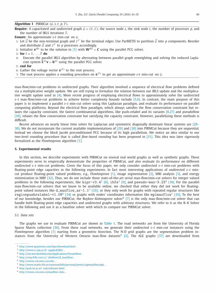
56 Y. Zhu, D.F. Gleich / Parallel Computing 59 (2016) 43–59

Table 2

Performance comparison between PIRMCut and B–K Solver. All the times are in seconds (rounded to integers). For

PIRMCut, we report the best total time and the number of cores p used.

Graph Platform p T PC T B-K T B-K / T PC δ

asia_osm Distributed memory 128 49 1465 29.8 3 . 4 × 10 −5

Shared memory 64 176 2158 12.3 3 . 0 × 10 −5

euro_osm Distributed memory 128 301 3102 10.3 6 . 8 × 10 −5

Shared memory 64 1248 4715 3.8 7 . 4 × 10 −5

adhead.n26c100 Distributed memory 128 167 555 3.3 7 . 0 × 10 −14

Shared memory 64 332 668 2 7 . 7 × 10 −14

bone.n26c100 Distributed memory 64 101 215 2.1 2 . 7 × 10 −14

Shared memory 64 200 248 1.2 2 . 7 × 10 −14

liver.n26c100 Distributed memory 128 88 294 3.3 9 . 0 × 10 −4

Shared memory 64 197 325 1.6 8 . 8 × 10 −4

graph_2007_000123_5 Distributed memory 32 22 4404 200 4 . 6 × 10 −3

Shared memory 32 28 2175 77.7 4 . 5 × 10 −3

graph_2007_000123_12 Distributed memory 32 73 202 2.8 2 . 3 × 10 −3

Shared memory 16 74 197 2.7 1 . 8 × 10 −3

graph_2007_000123_33 Distributed memory 32 16 68 4.3 2 . 0 × 10 −16

Shared memory 32 20 83 4.2 2 . 0 × 10 −16

wash-rlg-long.n2048.1163 Distributed memory 32 3 50 16.7 7 . 0 × 10 −2

Shared memory 64 2 84 42 7 . 0 × 10 −2

wash-rlg-long.n4096.1163 Distributed memory 32 6 199 33.2 7 . 0 × 10 −2

Shared memory 64 4 340 85 7 . 0 × 10 −2

wash-rlg-long.n8192.1163 Distributed memory 32 11 764 69.5 7 . 0 × 10 −2

Shared memory 32 9 1303 145 7 . 0 × 10 −2

wash-rlg-wide.n2048.1163 Distributed memory 32 29 457 15.8 1 . 4 × 10 −2

Shared memory 64 32 571 17.8 1 . 4 × 10 −2

wash-rlg-wide.n4096.1163 Distributed memory 64 255 – – –

Shared memory 64 334 – – –

wash-rlg-wide.n8192.1163 Distributed memory 32 10 – – –

Shared memory 32 9 – – –

the distributed memory machine. It’s interesting to observe that although the three graphs graph_2007_000123_5 ,graph_2007_000123_12 , and graph_2007_000123_33 are from the same sequence of related s –t min-cut prob-

lems, the times of the B–K Solver on them are dramatically different and unpredictable. In contrast, the times of PIRM-

Cut on these related problems are much more stable and predictable. On the two road networks, PIRMCut also achieves

desirable speed improvement over the B–K Solver. Notice that on the shared memory machine, if we extrapolate according

to the parallel speedup plot in Fig. 9 , the speed improvement of PIRMCut over the B–K Solver could be further continued

if we have more cores to utilize. For the DIMACS synthetic graphs Wash-Long and Wash-Wide, although they are of mod-

erate sizes, their floating point valued instances turn out to be very hard for the B–K Solver. It even did not terminate on

wash-rlg-wide.n4096.1163 and wash-rlg-wide.n8192.1163 after 4 hours on both the distributed and shared

memory machines. In comparison, PIRMCut could solve the Wash-Long and Wash-Wide problems very efficiently. The only

family of graphs on which we do not see a significant speed improvement using PIRMCut are the N-D grid graphs. This is

understood because the design and implementation of the B–K Solver is highly optimized for vision applications [7] . Ac-

cording to Table 2 , PIRMCut enables us to gain significant speed improvement by finding δ-accurate solutions. Moreover, for

some graphs PIRMCut could be the only feasible choice given the unpredictable and probably very high execution times of

B–K Solver.

For comparing the effectiveness of sweep cut and the two-level rounding procedure, we report their respective relative

approximation ratios on different graphs in Table 3 . It is shown that for each graph the sweep cut already produces a

reasonable approximate solution. In addition, on both the road networks and the N-D grid graphs, the two-level rounding

procedure consistently produces much better approximate solutions.

6. Discussion

The PIRMCut algorithm is a step towards our goal of a scalable, parallel s –t min-cut solver for problems with hundreds of

millions or billions of edges of which the capacities are floating-point valued. It has much to offer, and demonstrates good

scalability and speed improvement over an expertly crafted serial solver.

We have not yet discussed how to take advantage from solving a sequence of related s –t min-cut problems because we

have not yet completed our investigation into that setting. That said, we have designed our framework such that solving a

sequence of problems is reasonably straightforward. Note that all of the set up overhead of PIRMCut can be amortized when

solving a sequence of problems if the graph structure and edge capacities do not change dramatically. The larger issue with a

sequence of problems, however, is that our solver only produces δ-accurate solutions. For the applications where a sequence

is desired, we need to revisit the underlying methods and see if they can adapt to this type of approximate solutions. This

Y. Zhu, D.F. Gleich / Parallel Computing 59 (2016) 43–59 57

Table 3

Solution quality of sweep cut and the two-level rounding procedure. This table is based on the result on the dis-

tributed memory machine. The result on the shared memory machine is similar.

Graph Sweep cut Two-level

asia_osm 2 . 1 × 10 −3 3 . 4 × 10 −5

euro_osm 3 . 2 × 10 −2 6 . 8 × 10 −5

adhead.n26c100 1 . 0 × 10 −4 7 . 0 × 10 −14

bone.n26c100 9 . 7 × 10 −4 2 . 4 × 10 −14

liver.n26c100 4 . 9 × 10 −2 8 . 8 × 10 −4

graph_2007_000123_5 2 . 1 × 10 −2 4 . 6 × 10 −3

graph_2007_000123_12 2 . 4 × 10 −4 2 . 3 × 10 −3

graph_2007_000123_33 2 . 8 × 10 −11 5 . 2 × 10 −13

wash-rlg-long.n2048.1163 5 . 4 × 10 −2 7 . 0 × 10 −2

wash-rlg-long.n4096.1163 5 . 4 × 10 −2 7 . 0 × 10 −2

wash-rlg-long.n8192.1163 5 . 4 × 10 −2 7 . 0 × 10 −2

wash-rlg-wide.n2048.1163 4 . 4 × 10 −3 1 . 4 × 10 −2

setting also offers an opportunity to study the accuracy required for solving a sequence of problems. It is possible that by

solving each individual problem to a lower accuracy, it may generate a sequence with a superior final objective value for

application purposes. Alternatively, the method may be able to solve the cut problems to a fairly coarse accuracy much more

rapidly than existing exact solvers, and these approximations may suffice for many applications. Thus, the goal of our future

investigation on a sequence of problems will attempt to solve the sequence faster and better through carefully engineered

approximations.

There are also a few further investigations we plan to conduct regarding our framework. First, currently we used a pure

MPI based parallel PCG solver for the diagonally dominant Laplacians. Recent work on the nearly linear time solvers for such

systems shows the potential for fast runtime, but the parallelization potential is not yet evident in the literature. We wish to

explore the possibility of parallelizing these nearly linear time solvers as well as incorporating them into our framework. It is

also worthy to pursue a multithreaded implementation of PIRMCut. Given the recent advances in systems and architectures

targeted at irregular applications [12–14] , a multithreaded implementation of PIRMCut could obtain superior speedups on

these platforms.

Second, we wish to make our two-level rounding procedure more rigorous. As we have mentioned, this method is similar

to Lang’s flow-based rounding for the spectral method [31] that was later formalized in [1] . We hypothesize that a similar

formalization will hold here based on which we will be able to create a more principled approach. Furthermore, we suspect

that a multi-level extension of this will also be necessary as we continue to work on even larger problems.

Finally, we plan to continue working on improving the analysis of our PIRMCut algorithm in an attempt to formally bound

its runtime. This will involve designing more principled stopping criteria based on tighter diagnostics, e.g., from applying

our Cheeger-type inequality.

Acknowledgments

This work was partially supported by NSF CAREER award CCF-1149756 and ARO Award 1111691-CNS .

Appendix

We first prove the following characterization of λ2 .

Proposition A.1. λ2 is the optimal value of the constrained WLS problem

min

x

1

2 C x

T

Lx (A.1)

s.t. x s = 1 , x t = −1

Proof. By inspection, λ1 = 0 with x = e . Thus, λ2 can be represented by

λ2 = min

e T Dx =0

x

T Lx

x

T Dx

(A.2)

The constraint e T Dx = 0 is equivalent to x s + x t = 0 . Because the representation (A.2) is invariant to scaling of x , we can

constrain x s = 1 and x t = −1 , which results in x T Dx = 2 C. �

Note that (A.1) has a form similar to (5) , where the main difference is that we use { 1 , −1 } to encode the boundary

condition. We now prove the Cheeger-type inequality.

Theorem A.2. φ2 ≤ λ2 ≤ 2 φ

2

58 Y. Zhu, D.F. Gleich / Parallel Computing 59 (2016) 43–59

Proof. We first prove the direction of λ2 ≤ 2 φ. Let (S, S̄ ) be an s –t min-cut such that s ∈ S and t ∈ S̄ . Then φ(S) = φ. We

define the { 1 , −1 } encoded cut indicator vector

x u =

{1 if u ∈ S −1 if u ∈ S̄

This vector satisfies e T Dx = 0 . Then by representation (A.2)

λ2 ≤ x

T Lx

x

T Dx

=

4 cut(S, S̄ ) 2 C

= 2 φ(S) = 2 φ

We then prove the direction of φ2

2 ≤ λ2 . We follow the proof technique and notations used in Theorem 1 of [21] . Let g

denote the solution to (A.1) . Using an argument similar to Proposition 2.2 , we can show −1 ≤ g (u ) ≤ 1 . We sort the nodes

according to g such that

1 = g (s ) = g (v 1 ) ≥ · · · ≥ g (v n ) = g (t) = −1 (A.3)

Let S i = { v 1 , . . . , v i } for i = 1 , . . . , n − 1 and we denote by ˜ vol (S i ) = min { vol (S i ) , vol ( ̄S i ) } = C. We let α = min

n −1 i =1 φ(S i ) .

Generalizing the proof to Theorem 1 in [21] we can show

λ2 ≥(∑

u ∼v c({ u, v } )(g + (u ) 2 − g + (v ) 2 ) )2 (∑

u g + (u ) 2 d (u ) )(∑

u ∼v c({ u, v } )(g + (u ) + g + (v )) 2 )

To bound the denominator, we have ∑

u ∼v c({ u, v } )(g + (u ) + g + (v )) 2

≤2

∑

u ∼v c({ u, v } )(g + (u ) 2 + g + (v ) 2 ) ≤ 2 g + (s ) 2 d (s )

where the last inequality follows from g + (u ) ≤ g + (s ) and d (s ) = C = 2 ∑

u ∼v c({ u, v } ) . Because g + (t) = 0 and according to

the definition of (10) we have ∑

u g + (u ) 2 d (u ) = g + (s ) 2 d (s ) . By telescoping the term g + (u ) 2 − g + (v ) 2 using the ordering

(A.3) , we then have

λ2 ≥(∑ n −1

i =1 (g + (v i ) 2 − g + (v i +1 ) 2 ) cut(S i , S̄ i )

)2

2(g + (s ) 2 d (s )) 2

≥ α2

2

(∑ n −1 i =1 (g + (v i ) 2 − g + (v i +1 )

2 ) ̃ vol (S i ) )2

(g + (s ) 2 d (s )) 2 =

α2

2

where the last equality follows from

∑ n −1 i =1 (g + (v i ) 2 − g + (v i +1 )

2 ) ̃ vol (S i ) = g + (s ) 2 d (s ) because ˜ vol (S i ) = C = d (s ) for i =1 , . . . , n − 1 . From α ≥ φ we have λ2 ≥ φ2

2 . �

References

[1] R. Andersen , K.J. Lang , An algorithm for improving graph partitions, in: S.-H. Teng (Ed.), Proceedings of ACM-SIAM Symposium on Discrete Algorithms,

SIAM, 2008, pp. 651–660 . [2] Y. Boykov , G. Funka-Lea , Graph cuts and efficient N-D image segmentation, Int. J. Comput. Vis. 70 (2) (2006) 109–131 .

[3] D. Hernando , P. Kellman , J. Haldar , Z. Liang , Robust water/fat separation in the presence of large field inhomogeneities using a graph cut algorithm,

Magn. Reson. Med. 63 (1) (2010) 79–90 . [4] P. Christiano , J.A. Kelner , A. Madry , D.A. Spielman , S. Teng , Electrical flows, Laplacian systems, and faster approximation of maximum flow in undirected

graphs, in: Proceedings of Symposium on Theory of Computing, STOC, ACM, 2011, pp. 273–282 . [5] J.A. Kelner , Y.T. Lee , L. Orecchia , A. Sidford , An almost-linear-time algorithm for approximate max flow in undirected graphs, and its multicommodity

generalizations, in: Proceedings of ACM-SIAM Symposium on Discrete Algorithms, SIAM, 2014, pp. 217–226 . [6] Y.T. Lee , S. Rao , N. Srivastava , A new approach to computing maximum flows using electrical flows., in: Proceedings of Symposium on Theory of

Computing, STOC, ACM, 2013, pp. 755–764 .

[7] Y. Boykov , V. Kolmogorov , An experimental comparison of min-cut/max-flow algorithms for energy minimization in vision, IEEE Trans. Pattern Anal.Mach. Intell. 26 (9) (2004) 1124–1137 .

[8] B.V. Cherkassky , A.V. Goldberg , On implementing the push-relabel method for the maximum flow problem, Algorithmica 19 (4) (1997) 390–410 . [9] A.V. Goldberg , S. Hed , H. Kaplan , R.E. Tarjan , R.F. Werneck , Maximum flows by incremental breadth-first search, in: Proceedings of the 19th European

Conference on Algorithms, ESA’11, Springer-Verlag, 2011, pp. 457–468 . [10] D.S. Hochbaum , The pseudoflow algorithm: a new algorithm for the maximum flow problem, Oper. Res. 58 (4) (20 08) 992–10 09 .

[11] J. Nieplocha , A. Marquez , J. Feo , D.G. ChavarrÃa-Miranda , G. Chin , C. Scherrer , N. Beagley , Evaluating the potential of multithreaded platforms for

irregular scientific computations, in: U. Banerjee, J. Moreira, M. Dubois, P. Stenstrom (Eds.), Proceedings of International Conference on ComputingFrontiers, ACM, 2007, pp. 47–58 .

[12] J. Feo , D. Harper , S. Kahan , P. Konecny , Eldorado., in: N. Bagherzadeh, M. Valero, A. Ramirez (Eds.), Proceedings of International Conference on Com-puting Frontiers, ACM, 2005, pp. 28–34 .

[13] A. Tumeo , S. Secchi , O. Villa , Designing next-generation massively multithreaded architectures for irregular applications, IEEE Comput. 45 (8) (2012)53–61 .

Y. Zhu, D.F. Gleich / Parallel Computing 59 (2016) 43–59 59

[14] A . Morari , A . Tumeo , D.G. Chavarría-Miranda , O. Villa , M. Valero , Scaling irregular applications through data aggregation and software multithreading,in: Proceedings of the 28th IEEE International Parallel and Distributed Processing Symposium, IEEE, 2014, pp. 1126–1135 .

[15] A. Schrijver , Combinatorial Optimization – Polyhedra and Efficiency, Springer, 2003 . [16] A. Beck , On the convergence of alternating minimization for convex programming with applications to iteratively reweighted least squares and de-

composition schemes, SIAM J. Optim. 25 (1) (2015) 185–209 . [17] N. Vishnoi , Lx = b . Laplacian solvers and their algorithmic applications, Found. Trends Theor. Comput. Sci. 8 (1–2) (2012) 1–141 .

[18] M. Benzi , G.H. Golub , J. Liesen , Numerical solution of saddle point problems, Acta Numer. 14 (2005) 1–137 .

[19] R.S. Varga , Matrix Iterative Analysis, Second edition, Springer, 20 0 0 . [20] S. Toledo , H. Avron , Combinatorial preconditioners, in: U. Naumann, O. Schenk (Eds.), Combinatorial Scientific Computing, Chapman & Hall/CRC, 2012 .

[21] F. Chung , Four Cheeger-type inequalities for graph partitioning algorithms, in: Proceedings of International Conference on Cognitive Modeling, ICCM,2007 .

[22] I. Koutis, G. Miller, R. Peng, A generalized Cheeger inequality, 2014(Personal communication and public presentation). [23] Y. Saad , Iterative Methods for Sparse Linear Systems, SIAM, 2003 .

[24] G. Karypis , V. Kumar , A parallel algorithm for multilevel graph partitioning and sparse matrix ordering, J. Parallel Distrib. Comput. 48 (1) (1998) 71–95 .[25] G. Karypis , V. Kumar , Parallel multilevel k-way partitioning scheme for irregular graphs, SIAM Rev. 41 (2) (1999) 278–300 .

[26] A. Bhusnurmath , C.J. Taylor , Graph cuts via � 1 norm minimization, IEEE Trans. Pattern Anal. Mach. Intell. 30 (10) (2008) 1866–1871 .

[27] A.V. Goldberg , Two-level push-relabel algorithm for the maximum flow problem., in: A.V. Goldberg, Y. Zhou (Eds.), Proceedings of Conference onAlgorithmic Aspects in Information and Management, AAIM, Volume 5564 of Lecture Notes in Computer Science, Springer, 2009, pp. 212–225 .

[28] J.A. Kelner , L. Orecchia , A. Sidford , Z. Zhu , A simple, combinatorial algorithm for solving SDD systems in nearly-linear time, in: Proceedings of theForty-fifth Annual ACM symposium on Theory of computing, ACM, 2013, pp. 911–920 .

[29] I. Koutis , G.L. Miller , D. Tolliver , Combinatorial preconditioners and multilevel solvers for problems in computer vision and image processing, Comput.Vis. Image Underst. 115 (12) (2011) 1638–1646 .

[30] O.E. Livne , A. Brandt , Lean Algebraic Multigrid (LAMG): fast graph Laplacian solver, SIAM J. Sci. Comput. 34 (4) (2012) B499–B522 .

[31] K. Lang , Fixing two weaknesses of the spectral method., in: Proceedings of Neural Information Processing Systems, NIPS, 2005 . [32] V. Kolmogorov , R. Zabih , What energy functions can be minimized via graph cuts? IEEE Trans. Pattern Anal. Mach. Intell. 26 (2) (2004) 147–159 .

[33] A. Shekhovtsov , V. Hlavac , A distributed mincut/maxflow algorithm combining path augmentation and push-relabel, Int. J. Comput. Vis. 104 (3) (2013)315–342 .

[34] A. Delong , Y. Boykov , A scalable graph-cut algorithm for N-D grids, in: Proceedings of IEEE Conference on Computer Vision and Pattern Recognition,IEEE Computer Society, 2008 .

[35] P. Strandmark , F. Kahl , Parallel and distributed graph cuts by dual decomposition, in: Proceedings of IEEE Conference on Computer Vision and Pattern

Recognition, IEEE, 2010, pp. 2085–2092 . [36] T.A. Davis , Y. Hu , The University of Florida sparse matrix collection, ACM Trans. Math. Softw. 38 (1) (2011) 1 .

[37] C. Russell , L. Ladicky , P. Kohli , P.H.S. Torr , Exact and approximate inference in associative hierarchical networks using graph cuts, in: P. Grunwald,P. Spirtes (Eds.), Proceedings of Conference on Uncertainty in Artificial Intelligence, UAI, AUAI Press, 2010, pp. 501–508 .

[38] D.S. Johnson, C.C. McGeoch (Eds.), Network Flows and Matching: First DIMACS Implementation Challenge, American Mathematical Society, 1993 . [39] B. Smith , PETSc (portable, extensible toolkit for scientific computation), in: D.A. Padua (Ed.), Encyclopedia of Parallel Computing, Springer, 2011,

pp. 1530–1539 .

[40] T.A. Davis , Algorithm 832: UMFPACK V4.3—an unsymmetric-pattern multifrontal method, ACM Trans. Math. Softw. 30 (2) (2004) 196–199 .