A MIXED FINITE ELEMENT APPROXIMATION OF
STOKES-BRINKMAN AND NS-BRINKMAN EQUATION FOR
NON-DARCIAN FLOWS
INGRAM, R.N∗
Abstract.
We propose a finite element discretization of the Brinkman equation for modeling non-Darcianfluid flow by allowing the Brinkman viscosity ν → ∞ and permeability K → 0 in solid obstacles, andK → ∞ in fluid domain. In this context, the Brinkman parameters are generally highly discontinuous.Furthermore, we consider non-generic constraints: non-homogeneous Dirichlet boundary conditionsu|∂Ω = φ 6= 0 and non-solenoidal velocity ∇ · u = g 6= 0 (to model sources/sinks). Couplingbetween these two conditions makes even existence of solutions subtle. We establish well-posednessof the continuous and discrete problem, a priori stability estimates, and convergence as ν → ∞and K → 0 in solid obstacles, as K → ∞ in fluid region, and as the mesh width h → 0. Fornon-solenoidal Brinkman flows, we include a small data condition to ensure existence of solutions(idea applies directly to the steady Navier-Stokes equations). In addition, we propose a pseudo-skew-symmetrization of the discrete convective term
R
Ωu · ∇v · w required for analysis of discrete
non-solenoidal Brinkman problem.
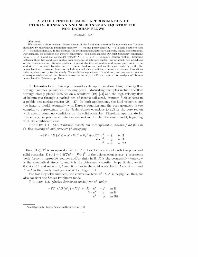
1. Introduction. This report considers the approximation of high velocity flowthrough complex geometries involving pores. Motivating examples include the flowthrough closely placed turbines on a windfarm [12], [24] and the high velocity flowof helium gas through a packed bed of (tennis-ball sized, uranium fuel) spheres ina pebble bed nuclear reactor [28], [27]. In both applications, the fluid velocities aretoo large to model accurately with Darcy’s equation and the pore geometry is toocomplex to approximate by the Navier-Stokes equations (NSE) in the pore regionwith no-slip boundary conditions on the solid obstacles. Therefore, appropriate forthis setting, we propose a finite element method for the Brinkman model, beginningwith the equilibrium case.
Problem 1.1. (NS-Brinkman model) For incompressible, viscous fluid flow inΩ, find velocity uδ and pressure pδ satisfying
−2∇ · (νD(uδ)) + uδ · ∇uδ + ∇pδ + νK−1uδ = f, in Ω
∇ · uδ = g, in Ωuδ = φ, in ∂Ω
Here, Ω ⊂ Rd is an open domain for d = 2 or 3 consisting of both the pores and
solid obstacles, D(uδ)
= 0.5(∇uδ +(∇uδ
)t) is the deformation tensor, f represents
body forces, g represents sources and/or sinks in Ω, K is the permeability tensor, νis the kinematical viscosity, and ν is the Brinkman viscosity. In particular, we fix0 < δ << 1 and set ν = 1/δ and K = 1/δ in the solid obstacles in Ω and ν = ν andK = δ in the purely fluid parts of Ω. See Figure 1.1.
For low Reynolds numbers, the convective term uδ · ∇uδ is negligible; thus, wealso consider the Stokes-Brinkman model.
Problem 1.2. (Stokes-Brinkman model) for uδ and pδ
−2∇ · (νD(uδ)) + ∇pδ + νK−1uδ = f, in Ω
∇ · uδ = g, in Ωuδ = φ, in ∂Ω
∗[email protected], http://www.math.pitt.edu/˜rni1
1
Ωf - The Fluid Domain
ν = νf
K = kf
SampleDomain − Ω = Ωf ∪ Ωp ∪ Ωs
Ωs
ν = νs
K = ks
K = kp
ν = νp
Ωp
Ωp
Ωs
Ωp
Ωp
Ωf
Ωfp = Ωf ∪ Ωp
Ωf
Ωs
Ωs
Ωfs = Ωf ∪ Ωs
Ωp
Ωp
Ωs
Ωs
Ωps = Ωp ∪ Ωs
Fig. 1.1. Sample subdomains Ω∗ ⊂ Ω with parameters ν∗, k∗, black regions not part of indicatedΩ∗. (top-left) Problem domain Ωfps = Ω, (top-right) Fluid-Porous domain Ωfp, (bottom-left) Fluid-Solid domain Ωfs, (bottom-right) Porous-Solid domain Ωps
For model parameters ν and K of order O(1), the numerical analysis of theBrinkman model fits within the framework for the abstract error analysis of the NSE,e.g. [11], [32]. However, the targeted applications of the Brinkman model are oftenhighly non-generic flows involving
• complex geometries, i.e. dense swarm of porous and solid obstacles• highly discontinuous parameters ν and K• non-homogeneous boundary conditions, i.e. uδ|∂Ω = φ 6= 0• general divergence conditions on velocity, i.e. ∇ · uδ = g 6= 0
Thus, we consider herein the numerical analysis associated with the asymptotic limitsand rates of convergence as the discretization parameter h δ tend to 0. The last twoconditions uδ|∂Ω 6= 0 and ∇·uδ 6= 0 in Ω are necessary for many natural and industrialflows in porous media.
We derive a weak formulation of Stokes and NS-Brinkman models in Section 2.Note that Hopf proved in [15] that solutions to the steady NSE exist for generalboundary data under certain restrictions on ∂Ω for the case ∇·u = 0. In Section 2.2,we note coupling between uδ|∂Ω = φ and ∇·uδ = g 6= 0 preventing a general existenceresult for nonzero boundary conditions and nonzero divergence. Our analysis is basedon the construction of an extension operator u of boundary data φ satisfying theconstraint ∇ · u = g. We show that for g ∈ L2 (Ω) and φ ∈ H1/2 (∂Ω) satisfying
• g ≡ 0, or• g has compact support in Ω,
∫
Ωg = 0, and g small enough, or
• g has compact support in Ω, and g and φ is small enough
2
there exists a solution(uδ, pδ
)∈ H1 (Ω) × L2 (Ω) to the NS-Brinkman Problem 1.1.
Furthermore, we show that the continuous (Section 2.3) and discrete (Section 3.1)Stokes- and NS-Brinkman models are well-posed (with small data for the nonlinearproblem). We derive a priori estimates for uδ with explicit dependence on ν, ν, andK. For δ > 0, both the continuous and discrete velocities for both Stokes-Brinkmanand NSE-Brinkman are of order O(
√δ/ν) in H1 in the solid obstacles embedded in Ω
and O(1/ν) in H1 in all Ω; hence, for fixed ν > 0, uδ is uniformly stable with respectto δ with respect to δ → 0.
For the numerical scheme, we provide a condition for interpolating non-smoothboundary data used in the analysis of the finite element discretization of the Brinkmanmodel. We also propose an innovative (explicitly pseudo-skew symmetrized, definedin Section 3, for general g) discrete form for the convective term u · ∇u . In Section3.1, we show that the proposed conforming finite element discretization provides aconvergent approximation uδ,h of uδ as h → 0 uniformly with respect to the penaltyparameter δ. In Section 3.2, letting u be a solution to the Stokes problem in thepurely fluid domain Ωf ⊂ Ω with no-slip boundary conditions on the solid obstacles,we show that the the discrete Brinkman velocity uδ,h converges to u as h, δ → 0 suchthat
∥∥uδ,h − u
∥∥
H1(Ω)≤ C
(δ
ν+∥∥uδ − uδ,h
∥∥
H1(Ω)
)
Finally, we provide numerical validations of our theory in Section 4.
1.1. Overview of Brinkman flow model. Whereas Darcy’s law assumes thatvelocity is proportional to the pressure gradient for a particular porous medium,Brinkman noted that, in general, the viscous effects must also be taken into accountto model flow accurately through porous media, see [6], [7]. Heuristic generalizationsof Darcy’s law have been considered to model non-Darcy flows in porous media (e.g.[14], [18], [26], [5]). Along with heuristic developments, theoretical justifications existfor the Brinkman model as an asymptotic approximation to the NSE, e.g. see [1], [16]and references therein. Straughan presents several of the most popular non-Darcymodels for flow in porous media in [30] (a well-cited compilation of his and others’contributions to this theory).
The Brinkman model has been applied to approximate non-Darcian flows in avariety of contexts; e.g. it is used to model oil filtration flows [17], groundwater flows[8], forced convective flows in metal foam-filled pipes (used in the cooling of electronicequipment) [23], gas diffusion through fuel cell membranes [13], Casson fluid flow inporous media (e.g. blood flow in vessels obstructed by fatty plaques and clots) [9],and interstitial fluid flow through muscle cells [31] with good accuracy. The Brinkmanequation is also used to model turbulence in porous media in the macroscopic scales[19] (for a discussion concerning turbulence modeling at the macroscopic versus themicroscopic pore level see [25]).
Numerical analysis of a discretization of the Stokes and NS-Brinkman flow modelis limited. In [33], Xie et.al. provide an innovative numerical analysis of the Stokes-Brinkman equations with a condition that ensures stable finite element spaces forthe discrete Stokes-Brinkman equation in the limiting condition for high Reynold’snumber. In [2], Angot provides a beautifully detailed error analysis for the continuousStokes-Brinkman fluid velocity in fluid-porous and fluid-solid domains compared toDarcy-Stokes velocities.
3
1.2. Approximating Brinkman flow in Ω. Solving the NSE in the pores of Ωwith no-slip boundary conditions at solid interfaces or non-stationary and/or complexdomain boundaries is cumbersome at best and most often simply not feasible [2], [3].Furthermore, the coupling condition between Stokes flow domains and Darcy flowdomains (used for flow in porous media) is physically unresolved even though theBeavers-Joseph-Saffman (BJS) interface condition is widely accepted and generallyused in practice [4], [29], [21]. Furthermore, Layton et.al show in [21] that coupledStokes-Darcy flow using the BJS interface condition is well-posed, but such a conclu-sion has not been verified for the nonlinear NS-Darcy coupling. In addition, furthercomplications arise because Stokes velocity has meaning of a ”pointwise” velocityand Darcy velocity has meaning of an ”averaged” velocity providing an unresolvedcompatability issue between these two velocities, see e.g. [18], [26], [5].
It is exactly these shortcomings in coupling Stokes or NSE with Darcy’s equa-tions that are the strengths of the Brinkman flow model. To this end, we considerthe penalized Brinkman problem formulated and described in [20] with convergenceanalysis in [2]. In particular, when approximating flows in Ω, we want uδ be as smallas possible inside all solid obstacles Ωs ⊂ Ω and recover the no-slip condition on eachsolid interface ∂Ωs. This is attained by imposing a large Brinkman viscosity ν andsmall permeability k in Ωs. In addition, in the purely fluid region Ωf ∈ Ω, there areno medium obstacles impeding the flow; thus, the permeability k in Ωf should belarge. Consider a small, parameter 0 < δ << 1 and set
ν|Ωs =ν
δ, k|Ωs = δ, k|Ωf
=1
δ
We are interested in the asymptotic behavior of solutions uδ to Problems 1.1 and 1.2 asδ → 0 and the double asymptotic of approximate solutions uδ,h as δ → 0, h→ 0. Thisfictitious domain approach has been analyzed in various contexts for the continuousBrinkman velocity uδ, see e.g. [2], [3], [19], [22]. The Brinkman approach eliminatesthe mathematical and physical problems with the interface couplings. Moreover, it issimple in implementation and easily adapted to existing computing platforms.
2. Problem formulation. We are interested in fluid flow through a porousmedium Ω, an open and connected domain in R
2 or R3, refer to Figure 1.1 for an
illustration. Decompose Ω into a purely fluid domain Ωf (no flow obstruction), porousdomain Ωp (some flow obstruction) and purely solid domain Ωs (complete flow ob-struction)
Ω = Ωf ∪ Ωp ∪ Ωs
where ∂Ωf , ∂Ωp, and ∂Ωs represent the corresponding boundaries of the indicatedsubdomains. We allow ∂Ω to be the union of distinct, connected segments. We assumethat ∂Ωp and ∂Ωs do not intersect with the problem domain boundary ∂Ω, thatΩp
and Ωs consist of open and connected subsets of Ω, and Ωp and Ωs are disjoint andbounded away from ∂Ω
Ωp ∩ Ωs = ∅,(Ωp ∪ Ωs
)∩ ∂Ω = ∅
Lastly, we require that Ωf is necessarily connected such that
∂Ωf = ∂Ω ∪ ∂Ωp ∪ ∂Ωs
4
We write Ω∗ for ∗ = f , p, s, fp, fs, ps, and fps such that
Ωfp := Ωf ∪ Ωp
Ωfs := Ωf ∪ Ωs
Ωps := Ωp ∪ Ωs
Ωfps := Ω
See Figure 1.1 for an illustration.
We assume that ν > 0 is constant in Ω. Also, ν > 0 is piecewise constant andconstant in each subdomain Ωf , Ωp, and Ωs such that ν|Ωf
= ν and ν|Ωp = ν. Wewrite
νf := ν|Ωf= ν, νp := ν|Ωp = ν, νs := ν|Ωs
See Figure 1.1 for an illustration. Moreover, we write
νfp (x) :=
νf , x ∈ Ωf
νp, x ∈ Ωp, νfs (x) :=
νf , x ∈ Ωf
νs, x ∈ Ωs, νps (x) :=
νp, x ∈ Ωp
νs, x ∈ Ωs
and identify ν = νfps (recall, Ωfps = Ω). The permeability tensor K ∈ L∞ (Ω)d×d
isgenerally symmetric and positive definite. We assume that K is a constant scalar oneach subdomain Ωf , Ωp, and Ωs and write
k∗ := K|Ω∗, ∗ = f , p, s, fp, fs, ps, and fps
and identify K = kfps. Lastly, for ∗ = f , p, s, fp, fs, ps, and fps write
ν∗max := maxx∈Ω∗
ν (x) , ν∗min := minx∈Ω∗
ν (x)
k∗max := maxx∈Ω∗
K (x) , k∗min := minx∈Ω∗
K (x)
and identify νmax := νfpsmax, νmin := νfps
min, kmax := kfpsmax, and kmax := kfps
max.
In porous regions Ωp, the Brinkman viscosity kp and νp should have moderatevalues. We suppose that kp depends on the domain geometry (e.g. see [5]). It is notwell understood how to select the Brinkman viscosity ν in Ωp. We set νfp = ν whichis a common choice in both engineering practice and analytical theory. See, e.g., [5]and [18] for more on this subject.
Lastly, assume that f ∈ H−1 (Ω)d
(the dual space of H10 (Ω)
dconsisting of H1-
functions vanishing on ∂Ω), φ ∈ H1/2 (∂Ω)d, and g ∈ L2 (Ω). We suppose that g is
localized satisfying
g ≡ 0 in Ωf ∪ Ωs
and compatible with the boundary data so that ∇ · uδ = g and thus
∫
Ω
g =
∫
∂Ω
φ · n (2.1)
In this context, we consider(uδ, pδ
)satisfying the nonlinear or linear system of equa-
tions, Problem 1.1, 1.2.
5
2.1. Weak formulation. Let V ′ denote the dual of any linear space V . Let∗ = f , p, s, fp, fs, ps, or fps. We write (·, ·)∗ to represent the L2 (Ω∗) inner productand (·, ·) when ∗ = fps (recall Ωfps = Ω). Let ‖·‖1,∗ represent standard norm for
H1 (Ω∗) and write ‖·‖∗ for the standard L2 (Ω∗)-norm, ‖·‖1 for the standard H1 (Ω)-norm (∗ = fps), and ‖·‖ for the standard L2 (Ω)-norm. Lastly, let 〈·, ·〉V ′×V representthe duality pairing for linear space V .
Definition 2.1. Let Ω∗ ⊂ Rd be an open set.
L20 (Ω∗) :=
q ∈ L2 (Ω∗) :∫
Ω∗
q = 0
, H10 (Ω∗) :=
v ∈ H1 (Ω∗) : v|∂Ω∗
= 0
Write Q := L20 (Ω) and X := H1
0 (Ω). For g ∈ L2 (Ω), φ ∈ H1/2 (∂Ω)
Xφ :=v ∈ H1 (Ω) : v|∂Ω = φ
Vφ (g) :=v ∈ Xφ :
∫
Ω q (∇ · v) =∫
Ω gq, ∀q ∈ L20 (Ω)
V ∗ :=
f ∈ X ′ : 〈f, v〉X′×H1
0
= 0, ∀v ∈ V0 (0)
V ⊥ :=v⊥ ∈ X :
∫
Ω v⊥ · v = 0, ∀v ∈ V0 (0)
and We write V = V0 (0), Vφ = Vφ (0), and V (g) = V0 (g). Moreover, X ′ =
H−1 (Ω) :=(H1
0 (Ω))′
is equipped with the following norm
‖f‖−1 = supv∈X,v 6=0
〈f, v〉X′×X
‖v‖1
Lastly, we note that Q′ = Q.If f ∈ L2 (Ω∗) and v ∈ H1 (Ω∗), we abuse notation and identify 〈f, v〉∗ = (f, v)∗
even though H−1 (Ω∗) is not the dual of H1 (Ω∗) (rather, it is the dual of H10 (Ω∗)).
Next, we define several (bi/tri)linear functionals:Definition 2.2. Let ∗ = f , p, s, fp, fs, or fsp. Let u, v, w ∈ H1 (Ω), and
q ∈ L2 (Ω). Define the bilinear and linear forms a∗ (·, ·), b∗ (·, ·), l2 (·) by
a∗ (·, ·) : H1 (Ω) ×H1 (Ω) → R, a∗ (u, v) :=∫
Ω∗
ν∇u : ∇v +∫
Ω∗
νK−1u · vb∗ (·, ·) : H1 (Ω) × L2 (Ω) → R, b∗ (v, q) := −
∫
Ω∗
q (∇ · v)l2,∗ (·) : L2
0 (Ω) → R, l2,∗ (q) := −∫
Ω∗
gq
Further, define the linear form l1,∗ (·) : H10 (Ω) → R,
l1,∗ (v) := 〈f, v〉H−1(Ω∗)×H1
0(Ω∗) −
∫
Ω∗νg∇ · v
and trilinear form c∗ (·, ·, ·) : H1 (Ω) ×H1 (Ω) ×H1 (Ω) → R,
c∗ (u, v, w) :=
∫
Ω∗
u · ∇v · w
To derive the variational formulation of Problems 1.1 and 1.2, we notice note that∇ · ∇ut = ∇(∇ · u). Consequently,
∇ ·(D(uδ))
=1
2
(∆uδ + ∇∇ · uδ
)=
1
2∆uδ +
1
2∇g
The term ∇g is data and included in l1 (·)). Thus, we have the following weak formu-lation of the NS-Brinkman equations, Problem 1.1.
6
Problem 2.3. (Weak NS-Brinkman) Given f ∈ X ′ and g ∈ L2 (Ω). Finduδ ∈ Xφ, pδ ∈ Q such that
∀v ∈ X, a(uδ, v
)+ b
(v, pδ
)+ c
(uδ, uδ, v
)= l1 (v)
∀q ∈ Q, b(uδ, q
)= l2 (q)
Similarly, the following variational formulation of Stokes-Brinkman equations, Prob-lem 1.2, follows by setting the convective term c (·, ·, ·) = 0 in Problem 2.3.
Problem 2.4. (Weak Stokes-Brinkman) Given f ∈ X ′ and g ∈ L2 (Ω). Finduδ ∈ Xφ, pδ ∈ Q such that
∀v ∈ X, a(uδ, v
)+ b
(v, pδ
)= l1 (v)
∀q ∈ Q, b(uδ, q
)= l2 (q)
Alternatively, we can formulate the variational Brinkman problem in operatornotation.
Definition 2.5. For any u, v ∈ H1 (Ω), w ∈ X, and q ∈ Q, define A ∈L (X ;X ′), B ∈ L (X ;Q), and C (u) ∈ L (X ;X ′) such that
〈Au,w〉X′×X := a (u, v)〈Bw, q〉Q×Q := b (w, q) =: 〈B′q, w〉X′×X
〈C (u) v, w〉X′×X := c (u, v, w)
Thus, we can rewrite Problem (2.3): find u ∈ Xφ, p ∈ Q satisfying
Au+B′p+ C (u)u = f (in X ′), Bu = g (in Q)
We can also rewrite Problem (2.4): find u ∈ Xφand p ∈ Q satisfying
Au+B′p = f (in X ′), Bu = g (in Q)
2.2. Calculus on subdomains Ω∗. We often decompose Ω into its physicalcomponents the purely fluid region Ωf , the porous region Ωp, and solid region Ωs. Indoing so, we must be careful in applying Poincare’s Inequality (since we require thatfunctions vanish on a set of positive measure on the domain boundary) and dualitypairing (since H−1 (Ω∗) is dual to H1
0 (Ω∗) and not toH1 (Ω∗)). We state these resultsin the context of our problem.
Theorem 2.6. (Poincare’s Inequality) For any w ∈ H10 (Ω), there exists C∗
p > 0such that
‖w‖Ω∗
≤ C∗p ‖∇w‖Ω∗
, for ∗ = f, fp, fs, fps
We generically write Cp = C∗p for all ∗.
Note that this result is not applicable in Ωs or Ωp since boundary data is generallynot provided on ∂Ωp or ∂Ωs. Additionally, the functional f ∈ H−1 (Ω∗) acts onelements from its dual space v ∈ H1
0 (Ω∗). Again, since boundary data is generallynot provided on ∂Ωp or ∂Ωs and
‖f‖−1,∗ = supv∈X(Ω∗),v 6=0
〈f, v〉X′×X
‖v‖1,∗
then 〈f, v〉H−1(Ω∗)×H1
0(Ω∗) ≤ ‖f‖−1,∗ ‖v‖1,∗ only applies when ∗ = fps.
7
Next, we collect some basic properties of the divergence operator.Lemma 2.7. For Ω ⊂ R
d open and connected the divergence operator is anisomorphism between V ⊥ and L2
0 (Ω). Therefore, there exists β > 0 such that theinf-sup condition holds:
infq∈L2
0(Ω)
supv∈H1
0(Ω)
〈∇q, v〉‖q‖ ‖v‖1
≥ β > 0. (2.2)
As a consequence, for any q ∈ L20 (Ω) there exists a unique v ∈ V ⊥ ⊂ H1
0 (Ω) satisfying
‖v‖1 ≤ β−1 ‖q‖ (2.3)
Proof. See, for example, page 24, Corollary 2.4 in [11] .
2.3. Decoupling ∇ · u = g and u|Ω = φ. It is necessary to rewrite the generaldivergence, nonhomogeneous Brinkman problems 1.2 and 1.1 in terms of a divergence-free velocity vanishing on the boundary ∂Ω. We compile several well-known results,e.g. see [11]. Recall that φ ∈ H1/2 (Ω), f ∈ X ′, and g ∈ L2 (Ω) satisfies the compati-bility condition Eq. (2.1). From from the trace theorem, there exists an extension
∃uφ ∈ H1 (Ω) satisfying uφ|∂Ω = φ (2.4)
and ∃γ > 0 such that ‖uφ‖1 ≤ γ ‖φ‖1/2,∂Ω (2.5)
Furthermore, from the compatibility condition Eq. (2.1) along with application of thedivergence theorem, we have that
∫
Ω(g −∇ · uφ) = 0. Hence, g−∇·uφ ∈ Q. Lemma
2.6 ensures that ∇ · : V ⊥ → Q defines an isomorphism so that
∃!u0 ∈ V ⊥ ⊂ X satisfying ∇ · u0 = g −∇ · uφ (2.6)
Hence, we consider looking for w ∈ V rather than uδ ∈ Vφ (g) solving Problems2.3 or 2.4.
Proposition 2.8. Given φ ∈ H1/2 (∂Ω) and g ∈ L2 (Ω) satisfying the compati-bility condition (2.1), suppose that uφ and u0 are defined as above in Eq.’s (2.4) and(2.6) respectively. Then writing u := uφ + u0,
‖u‖1 = ‖uφ + u0‖1 ≤(
γ +√dβ−1
)
‖φ‖1/2,∂Ω + β−1 ‖g‖ (2.7)
Moreover, solving Problems 2.3 and 2.4 for uδ ∈ Vφ (g) is equivalent to solving thesame equations for w ∈ V where
uδ = w + uφ + u0, ∇ · w = 0 in Ω, w|∂Ω = 0 (2.8)
Proof. The proof of the first bound follows by applying bound (2.3) and Lemma2.6. The problem equivalency is obvious.
Unfortunately, this bound is unsatisfying . In particular, similar to the NSE, wemust control the problematic term
∫
Ωw · ∇u · w, where w ∈ V is as in Eq. (2.8) and
u satisfies u|∂Ω = φ and ∇ · u = g in Ω as in Eq. (2.4). Noting that
∫
Ω
w · ∇u · w = −∫
Ω
w · ∇w · u ≤ C ‖∇w‖2 ‖u‖L4(Ω) (2.9)
8
must be absorbed from the right-hand side to left-hand side (details follow in the nextsection), the following proposition is necessary in establishing existence of solutionsto NS-Brinkman, Problem 2.3 for arbitrary data φ ∈ H1/2 (∂Ω). This result buildsupon the subtle and technical work of Leray rigorously compiled by Hopf in [15] andelegantly presented by Raviart and Girault in [11] and Galdi in [10] and specificallyconcerns nonhomogeneous boundary data for the steady Navier-Stokes equations withdivergence-free constraint ∇ · u = 0. Particular care must be taken in a domain withholes when
∫
∂Ωi
uδ · n = 0 (2.10)
is not required on each connected component of the boundary ∂Ωi ⊂ ∂Ω, i = 1, . . . , l.We consider another interesting case when sources and sinks are present inside thecomputational domain itself, i.e. when ∇ · uδ = g 6= 0.
Proposition 2.9. Let Ω be an open, connected domain with piecewise Lipschitzboundary ∂Ω and suppose that ∂Ω satisfies the Hopf condition (2.10). Suppose thatφ ∈ H1/2 (∂Ω) and g ∈ L2 (Ω) satisfy the compatibility condition Eq. (2.1) and thatg = 0 in Ωs and Ωf and g 6= 0 in Ωp. Fix ε > 0. (1) There an extension uε
φ ∈ Xφ such
that uεφ = 0 in Ωp and Ωs. There also exists u0 ∈ H1
0 (Ωfp) with extension u0 = 0 in
Ωs such that ∇ · u0 = g −∇ · uεφ in Ω. In particular,
u = uεφ + u0 =
uεφ + u0 in Ωf
u0 in Ωp
0 in Ωs
and
‖u0‖1 ≤ ‖g‖p +∥∥∇ · uε
φ
∥∥
f
(2)If in addition∫
Ω g = 0, then there exists an extension uεφ ∈ Vφ such that uε
φ = 0
in Ωp and Ωs. There also exists u0 ∈ H10 (Ωfp) with extension u0 = 0 in Ωs such that
∇ · u0 = g. In particular,
u = uεφ + u0 =
uεφ in Ωf
u0 in Ωp
0 in Ωs
and
‖u0‖1 ≤ ‖g‖p
In both cases, for any ε0 > 0, there exists an ε > 0 such that
∥∥uε
φ
∥∥
L4(Ω)< ε0
Proof. Our proof follows the work of Raviart and Girault for divergence-free ve-locities and non-homogeneous Dirichlet boundary conditions in [11], page 287, Lemma2.3 (also see [10]). From Eq. (2.4), there exists an extension uφ of φ ∈ H1/2 (∂Ω)satisfying ‖uφ‖1 ≤ γ ‖φ‖1/2,∂Ω. In order to localize contributions of problem data, we
consider the cut-off function ψε ∈ C∞ (Ω)
described in [11]. Briefly, ψε is identically
9
zero for all points in Ω a certain ε-dependent distance away from ∂Ω and identically1 a certain ε-dependent distance close to ∂Ω and smoothly connected in between.Moreover, ‖ψεv‖1 < ∞ for all v ∈ H1 (Ω). For (1), take uε
φ := γεuφ. We can takeε > 0 small enough to ensure that uε
φ = 0 in Ωp and Ωs. In addition
∫
Ωfp
∇ · uεφ =
∫
∂Ω
φ · n =
∫
Ωfp
g
and hence g − ∇ · uεφ ∈ L2
0 (Ωfp). Thus, by Lemma 2.6, there exists a unique u0 ∈V ⊥ (Ωfp) ⊂ H1
0 (Ωfp) such that ∇ · u0 = g −∇ · uεφ. We extend u0 = 0 on Ωs. The
bound ‖u0‖1 ≤ β−1||g−∇·uεφ||fp follows from Lemma 2.6. For (2) refer again to [11]
for the existence of a particular extension u∗φ, such that for any ε > 0,
uεφ = ∇×
(ψεu
∗φ
)
defines another extension of φ satisfying ∇ · uεφ = 0. Now since g ∈ L2
0 (Ωp), as a
consequence of Lemma 2.6, there exists a unique u0 ∈ V ⊥ (Ωp) satisfying ∇ · u0 = g.Extend u0 = 0 on Ωf and Ωs. We can take ε > 0 small enough to ensure that uε
φ = 0on Ωp and Ωs. Let u = uε
φ +u0. The bound for u0 follows from Lemma 2.6. The finalresult follows from the specially constructed property of γε.
Note that for g ≡ 0 in Ω, the L4-norm of u can be made arbitrarily small. However,for general g ∈ L2 (Ω), then g and φ are coupled via the necessary compatibilitycondition Eq. (2.1); hence, there is no obvious way to control the size of ‖u‖L4(Ω)
which is required to control the size of the bound in (2.9).Note that for the Hopf extension, ‖u‖L4(Ω) → 0 as ε→ 0, but the bound on ‖u‖1
grows exponentially as ε→ 0.
2.4. Continuity and coercivity. We now proceed with some important boundson the previously defined functionals required in our proceeding stability and erroranalysis.
Lemma 2.10. The linear functionals l1 (·) and l2 (·) are continuous. In particular,for any v ∈ H1 (Ω) and q ∈ L2 (Ω),
l1 (v) ≤ ‖f‖−1 ‖v‖1 + νmax
√d ‖g‖ ‖∇v‖ , if v ∈ X
l2,∗ (q) ≤ ‖g‖∗ ‖q‖∗ , for ∗ = f , p, s, fp, fs, ps, or fps
Moreover, for ∗ = f , p, s, fp, fs, ps, or fps, if f ∈ L2 (Ω∗), and v = 0 on Γ∗ ⊂ ∂Ω∗that has positive measure with respect to boundary, then
l1,∗ (v) ≤ ‖f‖∗ ‖v‖∗ + ν∗max
√d ‖g‖∗ ‖∇v‖∗ ≤
(
Cp ‖f‖∗ + ν∗max
√d ‖g‖∗
)
‖∇v‖∗
Proof. Linearity for the functionals is obvious. Continuity follows by a directapplication of the duality for ‖·‖−1-norm result and Cauchy-Schwarz for the others
along with Poincare and the fact that ‖∇ · v‖ ≤√d ‖∇v‖ to obtain ‖·‖1.
Lemma 2.11. The bilinear functional b (·, ·) is continuous. In particular, for∗ = f , p, s, fp, fs, ps, or fps and for any v ∈ H1 (Ω), q ∈ L2 (Ω)
b∗ (v, q) ≤√d ‖∇v‖∗ ‖q‖∗ (2.11)
10
Proof. Bilinearity is obvious. Continuity follows by a direct application of Cauchy-Schwarz inequality and the fact that ‖∇ · v‖ ≤
√d ‖∇v‖.
Lemma 2.12. The bilinear functional a (·, ·) is continuous and coercive. In par-ticular, for ∗ = f , p, s, fp, fs, ps, or fps and for any u, v ∈ H1 (Ω)
a∗ (u, v) ≤ ν∗max ‖∇u‖∗ ‖∇v‖∗ + ν (k∗min)−1 ‖u‖∗ ‖v‖∗ ≤ α∗
1 ‖u‖1,∗ ‖v‖1,∗ (2.12)
and
a∗ (v, v) ≥ ν∗min
∫
∗ |∇v|2 + νmin (k∗max)−1 ∫
∗ |v|2 ≥ α∗
0 ‖v‖21,∗ , or
a∗ (v, v) ≥ ν∗
min
2Cp‖v‖2
1,∗ , if v = 0 on Γ∗(2.13)
where Γ∗ ⊂ ∂Ω∗ has positive measure with respect to boundary and
α∗1 = max ν∗max, νmax/k
∗min , α∗
0 = min ν∗min, ν/k∗max (2.14)
Proof. Bilinearity is obvious. Continuity follows by bounding problem parametersν, ν, and K and applying the Cauchy-Schwarz inequality. The coercivity conditionfollows once again by bounding the problem parameters and, for the second form,applying the Poincare inequality.
Lemma 2.13. The trilinear functional c (·, ·, ·) is continuous. In particular, for∗ = f , p, s, fp, fs, ps, or fps and for any u, v, w in H1 (Ω)
c∗ (u, v, w) ≤ C∗L ‖u‖1,∗ ‖∇v‖∗ ‖w‖1,∗ (2.15)
where C∗L > 0 only depends on Ω∗. Moreover,
c∗ (u, v, w) ≤ C∗L ‖∇u‖∗ ‖∇v‖∗ ‖∇w‖∗ , if u|Γ∗
1, w|Γ∗
2= 0 (2.16)
where Γ∗1, Γ∗
2 ⊂ ∂Ω∗ have positive measure with respect to the boundary. We writeCL = C∗
L for all ∗.Separately, if ∇ · u = g in Ω∗ and (u · n (v · w)) |∂Ω∗
= 0, then
c∗ (u, v, w) = −c∗ (u,w, v) −∫
Ω∗
g (v · w) , and hence (2.17)
c∗ (u, v, v) = −1
2
∫
Ω∗
g |v|2 (2.18)
We call c∗ (·, ·, ·) pseudo-skew symmetric. Moreover, if ∇ ·u = 0 in Ω∗, then c∗ (·, ·, ·)is actually skew-symmetric.
Proof. Trilinearity is obvious. The two continuity bounds are classical results.To prove the first identity, we make use of Einstein’s tensor notation for indices andvector/tensor operations: u ·∇v ·w = uivj,iwj . Apply the divergence theorem and thefact that (u · n (v · w)) |∂Ω∗
vanishes on ∂Ω∗. Skew-symmetry for div-free functionsthen follows easily.
We call c∗ (·, ·, ·) pseudo-skew symmetric because the function
(u, v, w) 7→ c∗ (u, v, w) +1
2
∫
Ω∗
g (v · w)
is skew-symmetric.Remark 2.14. Note that, b (·, ·) is uniformly continuous; a (·, ·) is uniformly
continuous when, for some C > 0 we restrict ν, ν and ‖K‖L∞(Ω) < C1 < ∞; a (·, ·)is uniformly coercive when, for some C0 > 0 we restrict ν, ν ≥ C0 > 0. Hence, forturbulent flows there is a question concerning stability as ν → 0. Xie et.al. in [33]discuss the numerical aspects of properly selecting stable finite element spaces.
11
2.5. Well-posedness of Stokes-Brinkman. First, we establish existence anduniqueness along with a priori estimates for the weak Stokes-Brinkman equationbefore proceeding with the NS-Brinkman equation. We suppose that f ∈ L2 (Ω),φ ∈ H1/2 (Ω), and that g ∈ L2 (Ω) (g 6= 0 in Ωp and g = 0 in Ωf , Ωs) satisfiesthe compatability condition Eq. (2.1) throughout. We are particularly interested inrigorously tracking the dependence of solutions uδ to Stokes-Brinkman on ν, K andν. In the next theorem we prove that
∥∥∇uδ
∥∥ ≤ O
(1ν
),
∥∥uδ∥∥
1,s≤ O
(√δ
ν
)
Theorem 2.15. (Well-posedness Stokes-Brinkman) There exists a unique(uδ, pδ
)∈
(Xφ, Q) satisfying Stokes-Brinkman, Problem 2.4. Let u be an extension of boundarydata φ ∈ H1/2 (Ω) satisfying ∇ · u = g ∈ L2 (Ω), e.g. see Proposition 2.8. Then(uδ, pδ
)satisfy
∥∥∇uδ
∥∥ ≤ 1
ν
√
Cδ ,∥∥uδ∥∥
1,s≤
√δ
ν
√
Cδ
where
Cδ := Cδ (f, u) := C
(
‖f‖2fp + δ ‖f‖2
s +ν2
kp‖u‖2
1,fp
)
where the constant C is independent of parameters ν, ν, and K.Proof. Restrict v ∈ V . Then l1 (v) = 〈f, v〉 and we have a (w, v) = 〈f, v〉−a (u, v).
By the (bi)linearity and continuity of l1 (·), a (·, ·) along with coercivity of a (·, ·) onΩ established in Lemmas 2.9 and 2.11 we apply Lax-Milgram theorem to establishexistence and uniqueness of w ∈ V ⊂ X . For such a w, we now note that a (w, v) +a (u, v) − 〈f, v〉 = 0 for any v ∈ V . Thus, Aw +Au− f ∈ V ∗. Eq. (2.6) implies thatB = ∇ : Q → V ∗ defines an isomorphism. This establishes existences of a uniquepδ ∈ Q such that Bpδ = Aw + Au− L1. Finally, to show that uδ = w + u is uniquesolution is an easily follows from the coercivity of a (·, ·) on Ω. For the estimates,since w ∈ V , apply bounds from Lemmas 2.9 and 2.11 and bound on u in Eq. (2.7)and (2.3)
α0 ‖w‖21 ≤ a (w,w) = 〈f, w〉 − a (u, w)
≤ ‖f‖−1 ‖w‖1 + α1 ‖u‖1 ‖w‖1
Divide by ‖w‖1 and α0. To obtain estimate for uδ, apply triangle inequality∥∥uδ∥∥
1≤
‖w‖1 + ‖u‖1. Finally, to bound pδ, take v ∈ X and solve for pδ
b(pδ, v
)= l1 (v) − a
(uδ, v
)≤(
‖f‖−1 +√dνmax ‖g‖
)
‖v‖1 + α1
∥∥uδ∥∥
1‖v‖1
To finish, apply the inf-sup condition, Eq. (2.2), to obtain∥∥pδ∥∥ ≤ β−1 sup
(b(pδ , v
)/ ‖v‖1
).
Fix small δ > 0 and set ν/νs, 1/kf , and ks = δ. Then to summarize, we havepreliminary bounds on uδ and pδ
∥∥uδ∥∥
1≤ 1
ν ‖f‖−1 +(
1νδ + 1
)‖u‖1
∥∥pδ∥∥ ≤ 1
β
(
‖f‖−1 +√dν ‖g‖p
)
+ νβ
∥∥uδ∥∥
1
12
The bound for uδ is unsatisfying since it is not uniform as δ → 0. For sharperbounds, require f ∈ L2 (Ω) and decompose Ω to its components Ω∗. Recall that‖w‖∗ ≤ Cp ‖∇w‖∗ for ∗ = f , fp and u = 0 in Ωs. Applications of Cauchy-Schwarzand Young’s inequalities provide,
ν ‖∇w‖2fp + νs ‖∇w‖2
s +∑
∗=f,p,s
ν
k∗‖w‖2
∗ = a (w,w) = 〈f, w〉 − a (u, w)
≤∑
∗=f,p,s
(‖f‖∗ ‖w‖∗) +∑
∗=f,p
(
ν∗ ‖∇u‖∗ ‖∇w‖∗ +ν
k∗‖u‖∗ ‖w‖Ω∗
)
≤ C2P
ν‖f‖2
fp +ν
4‖∇w‖2
fp +ks
ν‖f‖2
s +ν
4ks‖w‖2
s
+ ν ‖∇u‖2fp +
ν
4‖∇w‖2
fp +∑
∗=f,p
ν
k∗
(
‖u‖2∗ +
1
4‖w‖2
∗
)
Combining terms, and simplifying we have
ν ‖∇w‖2fp + αs
0 ‖w‖21,s ≤
2C2p
ν‖f‖2
fp +2ks
ν‖f‖2
s + 4αfp1 ‖u‖2
1,fp
Recall ν/νs, 1/kf , and ks = δ. Also, recall that ν < αs0 = ν/δ and kp < kf = 1/δ
such that
αfp1 = maxx∈Ωfp
ν, ν/k (x) ≤ ν/kp
Then
‖w‖21,s ≤ C
(δν2 ‖f‖2
fp + δ2
ν2 ‖f‖2s + δ
kp ‖u‖21,fp
)
‖w‖21 ≤ C
(1ν2 ‖f‖2
fp + δν2 ‖f‖2
s + 1kp ‖u‖2
1,fp
)
Applying the triangle inequality
‖u‖1,s ≤ ‖w‖1,s + ‖u‖1,s
recalling that u ≡ 0 in Ωs (for the bound in Ωs) and assuming that kp ≤ 1 (for thebound in Ω) proves the claim.
2.6. Well-posedness of NS-Brinkman. We shall prove existence using theLeray-Schauder fixed point theorem. This requires some preliminary notation andestimates for NS-Brinkman (2.3).
Definition 2.16. Let u ∈ H1 (Ω) be an extension of boundary data φ ∈ H1/2 (Ω)preserving ∇ · u = g ∈ L2 (Ω); e.g. consider (1) or (2), Proposition 2.8. Then, wedefine(1) T : X ′ → V such that T (f) := w where w ∈ V solves
∀v ∈ V, a (w, v) = l1 (v) − a (u, v)
(2) N : V → X ′ such that N (w) := f + ∇(νg) − u · ∇u− u · ∇w − w · ∇u− w · ∇w(3) F : V → V such that F := T N .
13
In order to apply Leray Schauder’s fixed point theorem, we show that F is acompact linear operator with a fixed point that satisfies NS-Brinkman, Problem 2.3.We prove this through the proceeding lemmas.
Lemma 2.17. T is a well-defined linear, continuous operator.Proof. T is clearly linear. Well-posedness and boundedness of T follows from The-
orem 2.14. Since T is a linear and bounded operator, it follows that T is continuous.
Lemma 2.18. For any w ∈ V , then N (w) ∈ H−d/4 (Ω) and N maps V → X ′
continuously.Proof. The Ladyzhenskaya inequalities imply that there exists
√CL > 0 such
that ‖w‖L4 ≤ √CL ‖w‖1. By the Sobolev embedding theorem, Hd/4 (Ω) → L4 (Ω);
hence, there exists C4,d > 0 satisfying ‖v‖L4 ≤ C4,d ‖v‖Hd/4 for any v ∈ Hd/4 (Ω).Now fixing v ∈ Hd/4 (Ω) it is straightforward to bound
∫
Ω w · ∇w · v,∫
Ω u · ∇w · v,∫
Ωw · ∇u · v,
∫
Ωu · ∇u · v by
(√CLC4,d
)‖w‖1 ‖w‖1 ‖v‖d/4. Dividing each of the
resulting inequalities by ‖v‖d/4 and taking the supremum over all v ∈ Hd/4 (Ω), we
get the desired conclusion. Continuity follows by expanding ‖N (u1) −N (u2)‖−d/4
and successively applying Cauchy-Schwarz, the definition of the negative, fractionalSobolev norm, and the fact that N is bounded.
Proposition 2.19. F is a compact operator.Proof. By the Rellich Lemma, H−d/4 (Ω) is compactly imbedded in H−1 (Ω).
Hence, we summarize,
H1 7−→N , cont.
H−d/4 →compact
H−1 7−→T , cont.
H1
Hence, F is compact as a continuous composition of a compact operator.Before concluding existence, we require the following technical result necessary to
control the size of of the troublesome term arising in proving existence and derivationof the a priori estimate for uδ.
Proposition 2.20. F is a compact operator.Proof. By the Rellich Lemma, H−d/4 (Ω) is compactly embedded in H−1 (Ω).
Hence, we summarize,
H1 7−→N , cont.
H−d/4 →compact
H−1 7−→T , cont.
H1
Hence, F is compact as a continuous composition of a compact operator.Before concluding existence, we require the following technical result necessary to
control the size of of the troublesome term arising in proving existence and derivationof the a priori estimate for uδ.
Lemma 2.21. Fix ε0 > 0. Consider boundary data φ ∈ H1/2 (∂Ω) and g ∈ L2 (Ω)satisfying the compatibility condition Eq. (2.1). For u defined by (1), Proposition 2.8,we have that for ε > 0 small enough
‖u‖L4(Ω∗) ≤√
CL
(
‖g‖p + 2√d ‖φ‖H1/2(∂Ω)
)
, ∗ = f , p (2.19)
Suppose further that∫
∂Ωφ · n = 0 and hence, g ∈ L2
0 (Ω). Then choosing u as in (2),Proposition 2.8, we have that for ε > 0 small enough
‖u‖L4(Ωf ) ≤ ε0 +√
CL ‖g‖p , ‖u‖L4(Ωp) ≤√
CL ‖g‖p
14
Proof. Apply Proposition 2.8 and Lemma 2.6.
Based on the definitions and lemmas above, we can conclude the following theo-rem.
Theorem 2.22. (Well-posedness NS-Brinkman) Suppose that the small datacondition is satisfied
2√
CL ‖u‖L4(Ωfp) ≤ν
2(2.20)
where u is an extension of boundary data φ ∈ H1/2 (Ω) satisfying ∇ · u = g ∈ L2 (Ω);e.g. consider (1) or (2), Proposition 2.8 with bounds provided in Lemma 2.20. Thenthere is at least one pair
(uδ, pδ
)∈ (Xφ, Q) satisfying NS-Brinkman, Problem 2.3 and
∥∥uδ∥∥
2
1,s≤ ν−2δCδ,NSE, or
∥∥uδ∥∥
1,s≤ O(ν−1
√δ)
∥∥∇uδ
∥∥
2 ≤ ν−2Cδ,NSE, or∥∥∇uδ
∥∥ ≤ O(ν−1)
where
Cδ,NSE := Cδ,NSE (u, f) := C
(
δ ‖f‖2s + ‖f‖2
fp +
(
ν2 +ν2
kp+ ‖u‖2
1,fp
)
‖u‖21,fp
)
and the constant C is independent of parameters ν, ν, and K. Furthermore, there is atmost one such solution
(uδ, pδ
)when the additional small data condition is satisfied:
12CL ‖g‖p +
√CL ‖u‖L4(Ωp) + ν−1CL
√Cδ,NSE ≤ 1
2αp0√
CL ‖u‖L4(Ωf ) + ν−1CL
√Cδ,NSE ≤ 1
2ν
ν−1CL
√Cδ,NSE ≤ 1
2νδ−3/2
(2.21)
Proof. We prove existence via the Leray-Schauder fixed point theorem. Fix v ∈ V .Then l1 (v) = 〈f, v〉 and Problem 2.3 becomes
a (w, v) + c (w,w, v) + c (w, u, v) + c (u, w, v) = 〈f, v〉 − a (u, v) + c (u, u, v)
It is easy to see that a fixed point of the nonlinear, compact operator F is a solutionof this variational problem. Thus, consider the family of fixed point problems: for any0 < λ ≤ 1, find uλ ∈ X0 satisfying uλ = λF (uλ). Noting that u ≡ 0 in Ωs and thepseudo-skew symmetry of c∗ (·, ·, ·) (Eq. (2.18)), applications of Holder’s and Young’s
15
inequalities provide
ν ‖∇uλ‖2fp + νs ‖∇uλ‖2
s +∑
∗=f,p,s
ν
k∗‖uλ‖2
∗
= λ
∑
∗=f,p,s
l1,∗ (uλ) − c∗ (uλ, uλ, uλ)︸ ︷︷ ︸
=0
+∑
∗=f,p
(−a∗ (u, uλ) − c∗ (u, u, uλ) − c∗ (uλ, u, uλ) − c∗ (u, uλ, uλ))
≤∑
∗=f,p,s
‖f‖∗ ‖uλ‖∗ +∑
∗=f,p
(
ν∗ ‖∇u‖∗ ‖∇uλ‖∗ +ν
k∗‖u‖∗ ‖uλ‖∗
)
+ CL ‖u‖21,fp ‖∇uλ‖fp + 2
√
CL ‖u‖L4(Ωfp) ‖∇uλ‖2fp
≤ ks
2ν‖f‖2
s +ν
2ks‖uλ‖s +
3C2p
ν‖f‖2
fp +ν
12‖∇uλ‖2
fp
+ 3ν ‖∇u‖2fp +
ν
12‖∇uλ‖2
fp +∑
∗=f,p
ν
2k∗
(
‖u‖2∗ + ‖uλ‖2
∗
)
+3C2
L
ν‖u‖4
1,fp +ν
12‖∇uλ‖2
fp + 2√
CL ‖u‖L4(Ωfp) ‖∇uλ‖2fp
Let u be one of the extensions in Proposition 2.8 so that we have bounds in Lemma2.20 and the first small data condition Eq. (2.20) satisfied. Absorbing terms andsimplifying, we obtain
ν ‖∇uλ‖2fp + αs
0 ‖uλ‖21,s
≤ ks
ν‖f‖2
s +6C2
p
ν‖f‖2
fp +
(
6ν +ν
kp+
6C2L
ν‖u‖2
1,fp
)
‖u‖21,fp
Recall ν/νs, 1/kf , and ks = δ and that ν < αs0 = ν/δ. Then,
‖∇uλ‖2fp ≤ C
(δν2 ‖f‖2
s + 1ν2 ‖f‖2
fp +(
1 + 1kp + 1
ν2 ‖u‖21,fp
)
‖u‖21,fp
)
‖uλ‖21,s ≤ C
(δ2
ν2 ‖f‖2s + δ
ν2 ‖f‖2fp +
(
δ + δkp + δ
ν2 ‖u‖21,fp
)
‖u‖21,fp
)
Thus, we have the necessary bound uniform in λ to conclude existence of w ∈ Vto homogeneous, NS-Brinkman via Leray-Schauder. Hence, there exists uδ = w + usatisfying Problem 2.3.
The stability bound for any solution w ∈ V to homogeneous NS-Brinkman issimilar and leads to the same result as for uλ. We recall that uδ = w + u. Thus,the stability bound for uδ follows by application of the triangle inequality,
∥∥uδ∥∥
1,∗ ≤‖w‖1,∗ + ‖u‖1,∗. Noting that u ≡ 0 in Ωs we prove the a priori estimate.
To establish uniqueness, suppose w1, w2 are two such solutions. Then subtractingthe corresponding equations for fixed v ∈ V , we get
0 = a (w1 − w2, v) + c (w1, w1, v) − c (w2, w2, v)
= a (w1 − w2, v) + c (w1 − w2, u, v) + c (u, w1 − w2, v)
16
Write w = w1 − w2 and take v = w (indeed, w ∈ V ). Recall that u ≡ 0 in Ωs andg ≡ 0 in Ωf . By rearranging the above equality, decomposing the domains, noting thepseudo-skew symmetry of c∗ (·, ·, ·) (Eq. (2.18)), and applying Holder’s and Young’sinequalities, we obtain
∑
∗=f,p,s
ν∗ ‖∇w‖2∗ +
ν
k∗‖w‖2
∗
=∑
∗=f,p,s
−c∗ (w,w2, w) +∑
∗=f,p
−c∗ (w, u, w) − c∗ (u, w, w)
=∑
∗=f,p,s
(−c∗ (w,w2, w)) +∑
∗=f,p
(−c∗ (w, u, w)) − 1
2
∫
Ωp
g |w|2
≤ CL
2‖g‖p ‖w‖
21,p +
∑
∗=f,p
√
CL ‖u‖L4(Ω∗) ‖w‖21,∗ +
∑
∗=f,p,s
CL ‖w2‖∗ ‖w‖21,∗
Thus, requiring
CL
2 ‖g‖p +√CL ‖u‖L4(Ωp) + 1
νCL
√Cδ,NSE < αp
0√CL ‖u‖L4(Ωf ) + 1
νCL
√Cδ,NSE < ν
√δ
ν CL
√Cδ,NSE < αs
0
is a sufficient condition to ensure w ≡ 0. Note that αs0 = ν/δ. Now set uδ = w + u.
Then uδ ∈ Vφ (g) satisfies the nonhomogeneous, NS-Brinkman. Suppose that thereare two such solutions u1 and u2. Then subtracting the corresponding equations forfixed v ∈ V , we get a (u1 − u2, v) + c (u1, u1, v) + c (u2, u2, v) = 0. Add/subtractc (u1, u2, v). Set v = u1 − u2 (indeed, (u1 − u2) |∂Ω = 0 and ∇ · (u1 − u2) = 0).Write w = u1 − u2. Recall again that g ≡ 0 in Ωfs. Then rearranging, noting thepseudo-skew symmetry of c∗ (·, ·, ·) (Eq. (2.18)), and applying Holder’s and Young’sinequalities, we obtain
∑
∗=f,p,s
ν∗ ‖∇w‖2∗ +
ν
k∗‖w‖2
∗ =∑
∗=f,p,s
c∗ (w, u1, w) + c∗ (u2, w, w)
=∑
∗=f,p,s
(c∗ (w, u1, w)) −∫
Ωp
g |w|2
≤ CL ‖g‖p
∥∥uδ∥∥
2
1,p+ CL ‖∇u1‖f ‖∇w‖2
f +∑
∗=p,s
(
CL ‖u1‖1,∗ ‖w‖21,∗
)
Thus, the following is a sufficient condition to ensure w ≡ 0
1νCL
√Cδ,NSE + ‖g‖p < αp
0,1νCL
√Cδ,NSE < ν, δ
νCL
√Cδ,NSE < αs
0
Hence, the second small data condition Eq. (2.21) is sufficient to ensure uniqueness.Establishing existence/uniqueness of pδ ∈ Q follows by applying usual techniquesderived from the inf-sup condition.
Note that in the case g ≡ 0, u0 ≡ 0 and thus ‖u‖L4(Ω) = ||uεφ||L4(Ω) can be taken
arbitrarily small. Returning to the application of Leray-Schauder fixed point theoremin the previous proof, we can apply this result to conclude existence for any data.
Remark 2.23. The question of existence for large data g ∈ L2 (Ω) is an openproblem. The difficulty is that there is an irrevocable coupling between the divergence
17
condition ∇ · uδ = g and the boundary data uδ|∂Ω = φ via the compatibility condition(2.1). By this compatibility condition and Lemma 2.6, we have that for any extensionuφ ∈ Xφ, there exists a unique u0 ∈ V ⊥ ∈ X satisfying ∇ · u0 = g − ∇ · uφ withonly a bound ‖u0‖1 available. In other words, even though through the Hopf extensionwe can control the size of ‖uφ‖L4(Ω), we have no obvious way to control the size of
‖u0‖L4(Ω) to an arbitrary degree as required in applying the first small data condition
(2.20) in the proof for existence in Theorem 2.21.
3. Convergence and consistency analysis. To derive a mixed finite elementformulation of continuous Brinkman, 2.4 and 2.3, assume that Ω is polygonal withpolygonal subdomains Ω∗ for ∗ = p, s. Let Th be a triangulation of Ω with Eh ∈ Th
triangles for d = 2 or tetrahedra for d = 3. Moreover, we require that any Eh ∈ Th
be such that interior(Eh) is completely contained in Ωf , Ωp, or Ωs.For non-homogeneous boundary data φ ∈ H1/2 (∂Ω), we consider associated in-
terpolant of this problem data φh satisfying∫
∂Ω
φ · n =
∫
∂Ω
φh · n (3.1)
which is required in this analysis, explicitly used in proving Lemma 3.7. Accordingly,we define the following general finite element spaces for our analysis
Xhφh :=
v ∈ C0 (Ω)d
: ∀Eh, v|Eh∈ (Pv)
d ∈ Th and v|∂Eh∩∂Ω = φh
Qh :=q ∈ L2
0 (Ω) : ∀Eh ∈ Th, q|Eh∈ Pq
for some finite dimensional spaces polynomial spaces Pv and Pq so that Xhφh ⊂ H1 (Ω)
and Qh ⊂ Q be conforming, finite element subspaces. We write Xh = Xh0 ⊂ X . For
example, let Xhφh and Qh be spaces of piecewise polynomials on each element of Th
that satisfy the discrete inf-sup condition
infq∈Qh
supv∈Xh
b (v, q)
‖v‖1 ‖q‖≥ βh > 0 (3.2)
The well-known Taylor-Hood mixed finite elements are one such example where Xh
consists of piecewise quadratic elements and Qh piecewise linears. We also define thediscrete analogue to Vφ (g).
V hφh (g) =
v ∈ Xhφh :
∫
Ω
(∇ · v) q =
∫
Ω
gq ∀q ∈ Qh
Write V hφh for g ≡ 0, V h (g) when φ ≡ 0, and V h with g and φ are 0. We consider the
general case V hφh (g) /∈ Vφ (g) (which is true for Taylor-Hood elements). We will also
need the following discrete analogue of the convective term.Definition 3.1. Fix g ∈ L2 (Ω) and u, v, w ∈ H1 (Ω) such that
∫
Ω(∇ · u) qh =
∫
Ω gqh for all qh ∈ Qh. Let ch∗ : H1 (Ω) ×H1 (Ω) ×H1 (Ω) → R be such that
ch∗ (u, v, w) :=1
2(c∗ (u, v, w) − c∗ (u,w, v)) − 1
2
∫
Ω∗
g (v · w)
By construction, ch∗ (·, ·, ·) is continuous, (explicitly) pseudo-skew symmetric, andconsistent with c∗ (·, ·, ·) in the sense stated in the following lemma.
18
Lemma 3.2. Fix g ∈ L2 (Ω). The trilinear functional ch (·, ·, ·) is continuous; inparticular, for u, v, w in H1 (Ω) such that
∫
Ω (∇ · u) qh =∫
Ω gqh for all qh ∈ Qh,
ch∗ (u, v, w) ≤ ChL ‖u‖1,∗ ‖v‖1,∗ ‖w‖1,∗
where ChL = CL
(
1 +√d/2)
. Write generically ChL := CL. Moreover,
ch∗ (u, v, v) = −1
2
∫
Ω∗
g |v|2 , ∇ · u = g ⇒ ch (u, v, w) = c (u, v, w)
Proof. Trilinearity of ch (·, ·, ·) is obvious. For continuity, first note that it is clearthat ‖g‖ ≤
√d ‖u‖1 (indeed, consider ‖g‖ = supq∈Qh ((∇ · u, q) / ‖q‖)). Then,
ch∗ (u, v, w) =1
2(c∗ (u, v, w) − c∗ (u,w, v)) − 1
2
∫
Ω∗
g (v · w)
≤ CL ‖u‖1,∗ ‖v‖1,∗ ‖w‖1,∗ +CL
2
(√d ‖u‖1,∗
)
‖v‖1,∗ ‖w‖1,∗
The other results are obvious applications of the definition of c∗ (·, ·, ·).We can now state the discrete NS-Brinkman problem:Problem 3.3. (Discrete NS-Brinkman) Fix f ∈ X ′ and g ∈ L2 (Ω) satisfying
the compatibility condition Eq. (2.1). Find uδ,h ∈ V hφh (g), pδ,h ∈ Qh satisfying
∀v ∈ Xh, a(uδ,h, v
)+ b
(v, pδ,h
)+ ch
(uδ,h, uδ,h, v
)= l1 (v)
∀q ∈ Qh, b(uδ,h, q
)= l2 (q)
Existence of solutions to the discrete NS-Brinkman, Problem 3.3, closely followsthe proof of for the continuous case. We conclude without further proof:
Theorem 3.4. (Well-posedness of Discrete NS-Brinkman) Under small dataconditions of Theorem 2.21, there exists a uniqe solution (uδ,h, pδ,h) ∈ (V h
φh (g) , Qh)of the Discrete NS-Brinkman, Problem 3.3 that satisfies the same stability bound asTheorem 2.14 with uδ, pδ, β, and CL replaced by uδ,h, pδ,h, βh, and Ch
L respectively.Write generically βh = β and Ch
L = CL.For low Reynold’s numbers, the convective term in NS-Brinkman is negligible.
Hence, taking ch (·, ·, ·) = 0, we consider the discrete analogue of Stokes-Brinkman.Problem 3.5. (Discrete Stokes-Brinkman) Fix f ∈ X ′ and g ∈ L2 (Ω) satisfying
the compatibility condition Eq. (2.1). Find uδ,h ∈ V hφh (g), pδ,h ∈ Qh satisfying
∀v ∈ Xh, a(uδ,h, v
)+ b
(v, pδ,h
)= l1 (v)
∀q ∈ Qh, b(uδ,h, q
)= l2 (q)
Existence of solutions to discrete Stokes-Brinkman, Problem 3.5, closely followsthe proof of for the continuous case. We conclude without further proof:
Theorem 3.6. (Well-posedness of Discrete NS-Brinkman) There exists a unique(uδ,h, pδ,h) ∈ (V h
φh (g) , Qh) satisfying discrete Stokes-Brinkman, Problem 3.5. More-over, any such solution satisfies the same stability bound as the continuous problemshown in Theorem 2.14 with uδ, pδ, β and CL replaced by uδ,h, pδ,h, βh, and Ch
L
respectively. Write generically βh = β and ChL = CL.
19
3.1. Convergence analysis of discrete Brinkman. We now derive errorestimates uδ,h obtained from both Problems 3.5 and (3.3). For what follows, let(uδ, pδ
)∈ (Vφ (g), Q) and
(uδ,h, pδ,h
)∈(
V hφh (g), Qh
)
represent solutions of the con-
tinuous NS-Brinkman (or Stokes-Brinkman) and discrete NS-Brinkman (or Stokes-Brinkman) problems respectively. We show that these error estimates for the discreteBrinkman velocity uδ,h relative to the continuous Brinkman velocity uδ are uniformwith respect to penalty parameter δ → 0.
The following lemma is a technical result required in proving the error estimate.Lemma 3.7.
infvh∈V h
φh (g)
∥∥uδ − vh
∥∥
1≤(
1 +
√d
βh
)
infvh∈Xh
φh
∥∥uδ − vh
∥∥
1
Proof. Fix vh ∈ Xhφh . By choosing a good approximation φh of boundary data
φ ∈ H1/2 (Ω) via Eq. (3.1), we ensure that ∇ ·(uδ − vh
)∈ L2
0 (Ω). Hence, as adiscrete analogue of Lemma 2.6 implied by the discrete inf-sup condition, there exists
wh ∈(V h)⊥
satisfying ∇ · wh = ∇ ·(uδ − vh
). Moreover,
∥∥wh
∥∥
1≤ 1
βhsup
q∈Qh
b(wh, q
)
‖q‖ =1
βhsup
q∈Qh
b((uδ − vh
), q)
‖q‖ ≤√d
βh
∥∥uδ − vh
∥∥
1
Since ∇ ·(wh + vh
)= ∇ · uδ = g, it follows that v∗h :=
(wh + vh
)∈ V h (g). Hence,
∥∥uδ − v∗h
∥∥
1≤∥∥uδ − vh
∥∥
1+∥∥wh
∥∥
1≤(
1 +
√d
βh
)
∥∥uδ − vh
∥∥
1
This inequality holds for arbitrary vh ∈ Xhφh , the conclusion follows.
We state the following error estimate for Stokes-Brinkman velocities.Theorem 3.8. (Stokes-Brinkman error estimate) Suppose that
(uδ, pδ
)∈ (Xφ, Q)
solves Stokes-Brinkman, Problem 2.4, and uδ,h ∈ Xhφh solves discrete Stokes-Brinkman,
Problem 3.5. Then,
∥∥∇(uδ − uδ,h
)∥∥
2 ≤ C
[
infqh∈Qh
(1ν2
∥∥pδ − qh
∥∥
2
fp+ δ
ν
∥∥pδ − qh
∥∥
2
s
)
+ infvh∈Xh
φh
((1 + 1
kp
) ∥∥uδ − vh
∥∥
2
1,fp+ 1
δ
∥∥uδ − vh
∥∥
2
1,s
)
∥∥uδ − uδ,h
∥∥
2
1,s≤ C
[
infqh∈Qh
((δν2
∥∥pδ − qh
∥∥
2
fp+ δ2
ν
∥∥pδ − qh
∥∥
2
s
))
+ infvh∈Xh
φh
δ((
1 + 1kp
) ∥∥uδ − vh
∥∥
2
1,fp+∥∥uδ − vh
∥∥
2
1,s
)
where C is independent of ν, K, ν.Proof. Fix vh ∈ V h. Note that
(q,∇ · vh
)= 0 for any q ∈ Qh. Then,
a(uδ, vh
)+ b
(pδ, vh
)= l1
(vh), and a
(uδ,h, vh
)= l1
(vh)
20
Fix uh ∈ V hφh (g). Let η := uδ − uh, φh := uh−uδ,h. Subtracting the above equations,
we get
a(φh, vh
)= −b
(pδ, vh
)− a
(η, vh
)
Take vh = φh (indeed, φh = uh −uδ,h ∈ V h). Applying Cauchy-Schwarz and Young’sinequalities, we obtain
∑
∗=f,p,s
ν∗∥∥∇φh
∥∥
2
∗ +ν
k∗∥∥φh
∥∥
2
∗ = −b(pδ, φh
)− a
(η, φh
)
≤∑
∗=f,p,s
√d∥∥pδ − ph
∥∥∗
∥∥∇φh
∥∥∗ + ν∗ ‖∇η‖∗
∥∥∇φh
∥∥∗ +
ν
k∗‖η‖∗
∥∥φh
∥∥∗
≤∑
∗=f,p,s
3d
2ν∗
∥∥∥∥pδ − pδ
h∥∥∥∥
2
∗+ν∗
6
∥∥∇φh
∥∥
2
∗ +3ν∗
2‖∇η‖2
∗ +ν∗
6
∥∥∇φh
∥∥
2
∗
+3C2
P ν
2(kf )2‖η‖2
f +ν
6
∥∥∇φh
∥∥
2
f+∑
∗=p,s
ν
2k∗
(
‖η‖2∗ +
∥∥φh
∥∥
2
∗
)
Recall ν/νs, 1/kf , and ks = δ.
ν∥∥∇φh
∥∥
2
fp+ αs
0
∥∥φh
∥∥
2
1,s
≤ 3d
ν
∥∥pδ − ph
∥∥
2
fp+ 3dδ
∥∥pδ − ph
∥∥
2
s+ 3ν
(
1 + C4pδ +
C2p
kp
)
‖∇η‖2fp +
4ν
δ‖∇η‖2
1,s
Also, recall that ν < αs0 = minx∈Ωs 1/δ, ν/δ. Then,
∥∥∇φh
∥∥
2 ≤ C[
1ν2
∥∥pδ − ph
∥∥
2
fp+ δ
ν
∥∥pδ − ph
∥∥
2
s
+(1 + δ + 1
kp
)‖∇η‖2
fp + 1δ ‖∇η‖2
1,s
]
∥∥φh
∥∥
2
1,s≤ C
[δν2
∥∥pδ − ph
∥∥
2
fp+ δ2
ν
∥∥pδ − ph
∥∥
2
s
+(δ + δ2 + δ
kp
)‖∇η‖2
fp + ‖∇η‖21,s
]
Applying the triangle inequality∥∥uδ − uδ,h
∥∥
1≤∥∥φh
∥∥
1+‖η‖1 nearly proves the claim.
However, since this holds for any ph ∈ Qh but only for uh ∈ V hφh (g), we still must
show that this holds for any uh ∈ Xhφh . This follows from Lemma 3.7.
We notice that the only problematic term remaining is the term
1
δ
∥∥uδ − vh
∥∥
2
1,s
We show that this is bounded with respect to δ → 0.Theorem 3.9. For a suitable approximation vh ∈ Xh
φh of uδ ∈ Xφ,
1
δ
∥∥uδ − vh
∥∥
2
1,s≤ C <∞
where, C is a generic constant independent of δ.Proof. From approximation theory we have that
∥∥uδ − vh
∥∥
1,s≤ C
∥∥uδ∥∥
1,s. From
Theorem 2.14 we have the stability bound∥∥uδ∥∥
2
1,s≤ Cδ which proves the claim
21
We can also conclude the following error estimate for NS-Brinkman, Problem 3.3.Theorem 3.10. (NS-Brinkman error estimate) Suppose that the small data con-
dition Eq. (2.21) is satisfied. Then,
∥∥uδ − uδ,h
∥∥
2
1,s≤ C inf
qh∈Qh
(δ
ν2
∥∥pδ − qh
∥∥
2
fp+δ2
ν
∥∥pδ − qh
∥∥
2
s
)
+ infvh∈Xh
φh
[
δ
(
1 +1
kp+Cδ,NSE
ν4δ
)∥∥uδ − vh
∥∥
2
1,fp+
(
1 +Cδ,NSE
ν4δ3)∥∥uδ − vh
∥∥
2
1,s
]
and
∥∥∇(uδ − uδ,h
)∥∥
2 ≤ C infqh∈Qh
(1
ν2
∥∥pδ − qh
∥∥
2
fp+δ
ν
∥∥pδ − qh
∥∥
2
s
)
+ infvh∈Xh
φh
[(
1 +1
kp+Cδ,NSE
ν4δ
)∥∥uδ − vh
∥∥
2
1,fp+
1
δ
(
1 +Cδ,NSE
ν4δ3)∥∥uδ − vh
∥∥
2
1,s
]
where C > 0 is independent of ν, ν, and K.Proof. Fix vh ∈ V h. Note that
(q,∇ · vh
)= 0 for any q ∈ Qh. Then,
a(uδ, vh
)+ b
(pδ, vh
)+ ch
(uδ, uδ, vh
)= l1
(vh)
a(uδ,h, vh
)+ ch
(uδ,h, uδ,h, vh
)= l1
(vh)
Fix uh ∈ V hφh (g). Define η := uδ − uh, φh := uh−uδ,h. Expanding the nonlinear term
we obtain:
−ch(uδ, uδ, vh
)+ ch
(uδ, uδ, vh
)
= −ch(η, uδ, vh
)− ch
(φh, uδ, vh
)− ch
(uδ,h, η, vh
)− ch
(uδ,h, φh, vh
)
Subtracting the above equations, we get
a(φh, vh
)= −b
(pδ , vh
)− a
(η, vh
)
− ch(η, uδ, vh
)− ch
(φh, uδ, vh
)− ch
(uδ,h, η, vh
)− ch
(uδ,h, φh, vh
)
Take vh = φh (indeed, φh = uh − uδ,h ∈ V h). Then, applying Holder’s and Young’sinequalities and the explicit skew-symmetry of ch∗ (·, ·, ·), we obtain
∑
∗=f,p,s
ν∗∥∥∇φh
∥∥
2
∗ +ν
k∗
∥∥φh
∥∥
2
∗
=∑
∗=f,p,s
−b∗(pδ − ph, φh
)− a∗
(η, φh
)
+∑
∗=f,p,s
−ch∗(η, uδ, φh
)− ch∗
(φh, uδ, φh
)− ch∗
(uδ,h, η, φh
)− ch∗
(uδ,h, φh, φh
)
≤∑
∗=f,p,s
√d∥∥pδ − ph
∥∥∗
∥∥∇φh
∥∥∗ + ν∗ ‖∇η‖∗
∥∥∇φh
∥∥∗ +
ν
k∗‖η‖∗
∥∥φh
∥∥∗
+∑
∗=f,p,s
CL
(∥∥uδ∥∥
1,∗ +∥∥uδ,h
∥∥
1,∗
)
‖η‖1,∗∥∥φh
∥∥
1,∗ + CL
∥∥uδ∥∥
1,∗
∥∥φh
∥∥
2
1,∗
+1
2‖g‖p
(
CL
∥∥∇φh
∥∥
2
fp
)
22
We have shown previously that uδ and uδ,h are bounded in H1 in Ω and Ωs (Theorem2.21) and denoted
∥∥uδ∥∥
1,s≤
√δ
ν
√Cδ,NSE ,
∥∥∇uδ
∥∥ ≤ 1
ν
√Cδ,NSE
Recall ν/νs, 1/kf , and ks = δ. Then,
∑
∗=f,p,s
ν∗∥∥∇φh
∥∥
2
∗ +ν
k∗∥∥φh
∥∥
2
∗
≤∑
∗=f,p,s
4d
ν∗
∥∥pδ − ph
∥∥
2
∗ +ν∗
16
∥∥∇φh
∥∥
2
∗ + 4ν∗ ‖∇η‖2∗ +
ν∗
16
∥∥∇φh
∥∥
2
∗
+∑
∗=f,p,s
(2ν
k∗‖η‖2
∗ +ν
8k∗
∥∥φh
∥∥
2
∗
)
+C2
LCδ,NSE
ν2
6
ν‖∇η‖2
fp +ν
12
(∥∥∇φh
∥∥
2
f+∥∥∇φh
∥∥
2
p
)
+C2
LCδ,NSEδ2
ν2
8
ν‖η‖2
1,s +ν
8δ
∥∥φh
∥∥
2
1,s+CL
2‖g‖p
∥∥φh
∥∥
2
1,p
+ CL1
ν
√
Cδ,NSE
(∥∥∇φh
∥∥
2
f+∥∥∇φh
∥∥
2
p
)
+ CL
√δ
ν
√
Cδ,NSE
∥∥φh
∥∥
2
1,s
Also, recall that ν < αs0 = ν/δ and kp < kf = 1/δ such that
αfp1 = maxx∈Ωfp
ν, ν/k (x) ≤ ν/kp
Applying the small data condition (sufficient condition for uniqueness of solutions toNS-Brinkman), Eq. (2.21), absorbing terms, and simplifying we obtain
αfp0 ‖φ‖1,fp + αs
0 ‖φ‖1,s
≤ 16dδ∥∥pδ − ph
∥∥
2
s+
(
16δ
ν+ 8
ν
δ+ 32C2
LCδ,NSEδ2
ν3
)
‖η‖21,s
+16d
ν
∥∥pδ − ph
∥∥
2
fp+
(
32ν + 16C2L
ν
kp+ 24C2
LCδ,NSE1
ν3
)
‖∇η‖2fp
Apply the triangle inequality to obtain estimate for uδ − uδ,h (e.g.∥∥uδ − uδ,h
∥∥ ≤
∥∥φh
∥∥+‖η‖). This nearly proves the claim. However, since this holds for any ph ∈ Qh
but only for uh ∈ V hφh (g), we still must show that this holds for any uh ∈ Xh
φh . Thisfollows easily from Lemma 3.7.
3.2. Approximating slow, viscous flow around solid obstacles. We as-sume that the Stokes equation for fluid flow in Ωf be the true flow velocity:
Problem 3.11. (Stokes) Find (u, p) ∈ Xf,φ ×Q where
Xf,φ :=v ∈ H1 (Ωf ) : v|∂Ω = φ and v|∂Ωs = 0
with boundary data u|∂Ω = φ ∈ H1/2 (∂Ω) and u|∂Ωs = 0 such that τ (u, p) ∈ L2 (∂Ωs)satisfying
∀v ∈ H1 (Ω) ,∫
Ωfν∇u : ∇v −
∫
Ωfp∇ · v +
∫
∂Ωs(τ (u, p) · n) · v = 〈f, v〉
∀q ∈ L20 (Ω) ,
∫
Ωfq∇ · u = 0
23
where
τ (u, p) · n := ν∇u · n− pn
Note that g ≡ 0 here. Also, we only require velocity test functions to vanish on ∂Ωand not on ∂Ωs. Hence, we require the inclusion of the boundary integral to properlymodel Stokes flow around solid obstacles.
In order to establish well-posedness of solutions to this variational Stokes problem,we insist that solutions satisfy (u, p) ∈ H2 (Ωf ) ×H1 (Ωf ) and with extension u ≡ 0,p ≡ 0 on Ωs, that (u, p) ∈ H1
0 (Ω) × L2 (Ω). This will be guaranteed for polygonalboundaries ∂Ω, ∂Ωs and f ∈ L2 (Ω).
Consider approximations to this flow given by the discrete Stokes-Brinkman equa-tion,
(uδ,h, pδ,h
)∈ H1
0 (Ω) × L20 (Ω) solving Problem 3.5. First, we construct a priori
estimates for u in Ωf and uδ,h in Ωs.
Lemma 3.12. For f ∈ L2 (Ω), any solution u of the variational Stokes problemsuch that σ (u, p) ∈ L2 (∂Ωs) satisfies
‖∇u‖Ωf≤ C
1
ν‖f‖f
Here, C > 0 is a constant depending solely on the domain geometry.
Proof. Taking v = u in the variational Stokes equation, the result follows easily.
Proposition 3.13. Fix 0 < δ << 1. Assume ksmin, ks
max = δ and νs = ν/δ.Any solution uδ,h of the discrete Stokes-Brinkman problem satisfies
1
δ
∥∥∇uδ,h
∥∥
2
s+ν
δ
∥∥uδ,h
∥∥
2
s≤ C
(1
ν2‖f‖2
f +δ
ν2‖f‖2
s +1
νγ ‖φ‖H1/2(∂Ω)
)
Proof. Follows from work in previous section.
We want to exploit the relationship between approximations uδ,h to Stokes-Brinkman in Ω and solutions to the Stokes equations u in Ωf with extension u|Ωs ≡ 0.To this end, we reference Angot’s fundamental paper [2] in which he provides a cleverproof to establish a sharp estimate for
∥∥uδ − u
∥∥
1where uδ is the solution to continu-
ous Stokes-Brinkman in Ω. We state the theorem here in a slightly modified form toextract exact dependency of estimate on problem data.
Theorem 3.14. (Angot) Fix 0 < δ << 1. Assume ksmin, ks
max = δ and νs = ν/δ.Let (u, p) be a solution of the Stokes problem.
∥∥uδ − u
∥∥
1≤ C
δ
ν
(
‖f‖+ ‖τ‖H1/2(∂Ωs)
)
where we write τ := τ (u, p) and C > 0 is a constant independent of problem data ν,ν, K, f , φ.
Proof. Fix 0 < δ < 1. Let νf = ν, νs = ν/δ, kf = 1/δ, and ks = δ. Start withthe variational Brinkman problem: find uδ ∈ V satisfying a
(uδ, v
)= 〈f, v〉 for all
v ∈ V . Subtracting the variational Stokes problem from this, writing w = uδ − u we
24
have∫
Ωf
|∇w|2 +1
δ
∫
Ωs
|∇w|2 + δ
∫
Ωf
|w|2 +1
δ
∫
Ωs
|w|2
=1
ν
∫
Ωs
f · w − 1
ν
∫
∂Ωs
(τ (u, p) · n) · w − δ
∫
Ωf
u · w
≤ 1
ν2
δ
2‖f‖2
s +1
2δ‖w‖2 +
C
ν2
δ
2‖τ (u, p)‖2
H1/2(∂Ωs)
+1
2δ‖∇w‖2
s +δ
2‖u‖2
f +δ
2‖w‖2
f
Here, we bounded the right-hand side by successive applications of the Cauchy-Schwarz and Young inequalities. Absorbing terms right to left sides we obtain
∥∥∇(uδ − u
)∥∥
2
1≤ Cδ
(1ν2 ‖f‖2
+ 1ν2 ‖τ‖2
H1/2(∂Ωs)
)
∥∥uδ − u
∥∥
1,s≤ Cδ2
(1ν2 ‖f‖2
+ 1ν2 ‖τ‖2
H1/2(∂Ωs)
)
To recover optimal convergence in H1 (Ω) (i.e. to match the O (δ) convergencerate obtained in H1 (Ωs)), the idea is to avoid Young’s inequality and hence boundthe left-hand side by a factor of ‖w‖1. To this end, Angot considers the followingauxiliary problem: Find (ω, θ), where we write ωs := ω|Ωs , ωf := ω|Ωf
, θs := p∗|Ωs ,and θf := p∗|Ωf
, satisfying
− ν∆ωs + ∇θs + νωs = fs, ∇ · ωs = 0, in Ωs
τ (ωs, θs) · n|∂Ωs = τ (u, p) · n|∂Ωs
and
− ν∆ωf + ∇θf = 0, ∇ · ωf = 0, in Ωf
ωf |∂Ω = 0, ωf |∂Ωs = ωs|∂Ωs
The problem in Ωf is obviously well-posed from classical Stokes theory. The well-posedness of problem in Ωs is more subtle due to the boundary conditions on ∂Ωs.Considering the variational problem for ωs and ωf and the decomposition uδ = u+δω− z, a weak formulation for z can be established and through usual techniques, wecan recover an energy equation for z
‖∇z‖2f +
1
δ‖∇z‖2
s + δ ‖z‖2f +
1
δ‖z‖2
s
= δ
∫
Ωf
∇ω : ∇z + δ
∫
Ωf
u · z + δ2∫
Ωf
ω · z
≤(
δ ‖∇ω‖f + δ ‖u‖f + δ2 ‖ω‖f
)
‖∇z‖1,f
We note in addition to Angot’s work, that
‖∇ω‖f ≤ C ‖ωs‖1 ≤ 1
ν‖f‖s +
1
ν‖τ (u, p)‖H1/2(∂Ωs)
So, it follows that, with an application of Poincare-Friedrich’s inequality,
∥∥uδ − u
∥∥
1≤ δ ‖ω‖1 + ‖z‖1 ≤ C
δ
ν
(
‖f‖ + ‖τ‖H1/2(∂Ωs)
)
25
h∥∥uδ,h − uδ
∥∥
∣∣uδ,h − uδ
∣∣1
Rate (H1)
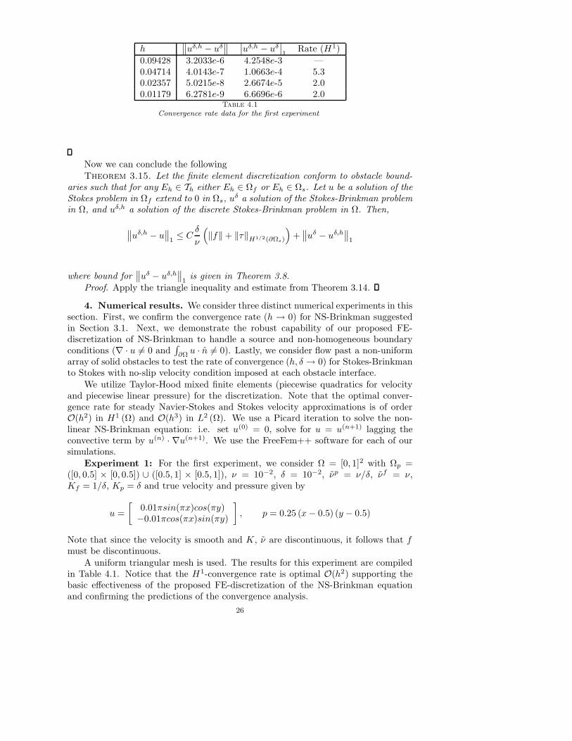
0.09428 3.2033e-6 4.2548e-3 —0.04714 4.0143e-7 1.0663e-4 5.30.02357 5.0215e-8 2.6674e-5 2.00.01179 6.2781e-9 6.6696e-6 2.0
Table 4.1
Convergence rate data for the first experiment
Now we can conclude the following
Theorem 3.15. Let the finite element discretization conform to obstacle bound-aries such that for any Eh ∈ Th either Eh ∈ Ωf or Eh ∈ Ωs. Let u be a solution of theStokes problem in Ωf extend to 0 in Ωs, u
δ a solution of the Stokes-Brinkman problemin Ω, and uδ,h a solution of the discrete Stokes-Brinkman problem in Ω. Then,
∥∥uδ,h − u
∥∥
1≤ C
δ
ν
(
‖f‖ + ‖τ‖H1/2(∂Ωs)
)
+∥∥uδ − uδ,h
∥∥
1
where bound for∥∥uδ − uδ,h
∥∥
1is given in Theorem 3.8.
Proof. Apply the triangle inequality and estimate from Theorem 3.14.
4. Numerical results. We consider three distinct numerical experiments in thissection. First, we confirm the convergence rate (h → 0) for NS-Brinkman suggestedin Section 3.1. Next, we demonstrate the robust capability of our proposed FE-discretization of NS-Brinkman to handle a source and non-homogeneous boundaryconditions (∇ · u 6= 0 and
∫
∂Ω u · n 6= 0). Lastly, we consider flow past a non-uniformarray of solid obstacles to test the rate of convergence (h, δ → 0) for Stokes-Brinkmanto Stokes with no-slip velocity condition imposed at each obstacle interface.
We utilize Taylor-Hood mixed finite elements (piecewise quadratics for velocityand piecewise linear pressure) for the discretization. Note that the optimal conver-gence rate for steady Navier-Stokes and Stokes velocity approximations is of orderO(h2) in H1 (Ω) and O(h3) in L2 (Ω). We use a Picard iteration to solve the non-linear NS-Brinkman equation: i.e. set u(0) = 0, solve for u = u(n+1) lagging theconvective term by u(n) · ∇u(n+1). We use the FreeFem++ software for each of oursimulations.
Experiment 1: For the first experiment, we consider Ω = [0, 1]2 with Ωp =([0, 0.5] × [0, 0.5]) ∪ ([0.5, 1] × [0.5, 1]), ν = 10−2, δ = 10−2, νp = ν/δ, νf = ν,Kf = 1/δ, Kp = δ and true velocity and pressure given by
u =
[0.01πsin(πx)cos(πy)−0.01πcos(πx)sin(πy)
]
, p = 0.25 (x− 0.5) (y − 0.5)
Note that since the velocity is smooth and K, ν are discontinuous, it follows that fmust be discontinuous.
A uniform triangular mesh is used. The results for this experiment are compiledin Table 4.1. Notice that the H1-convergence rate is optimal O(h2) supporting thebasic effectiveness of the proposed FE-discretization of the NS-Brinkman equationand confirming the predictions of the convergence analysis.
26
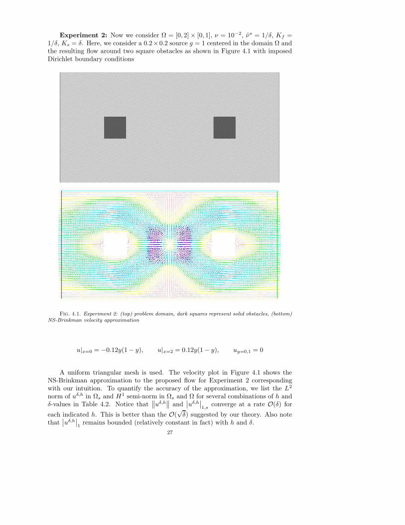
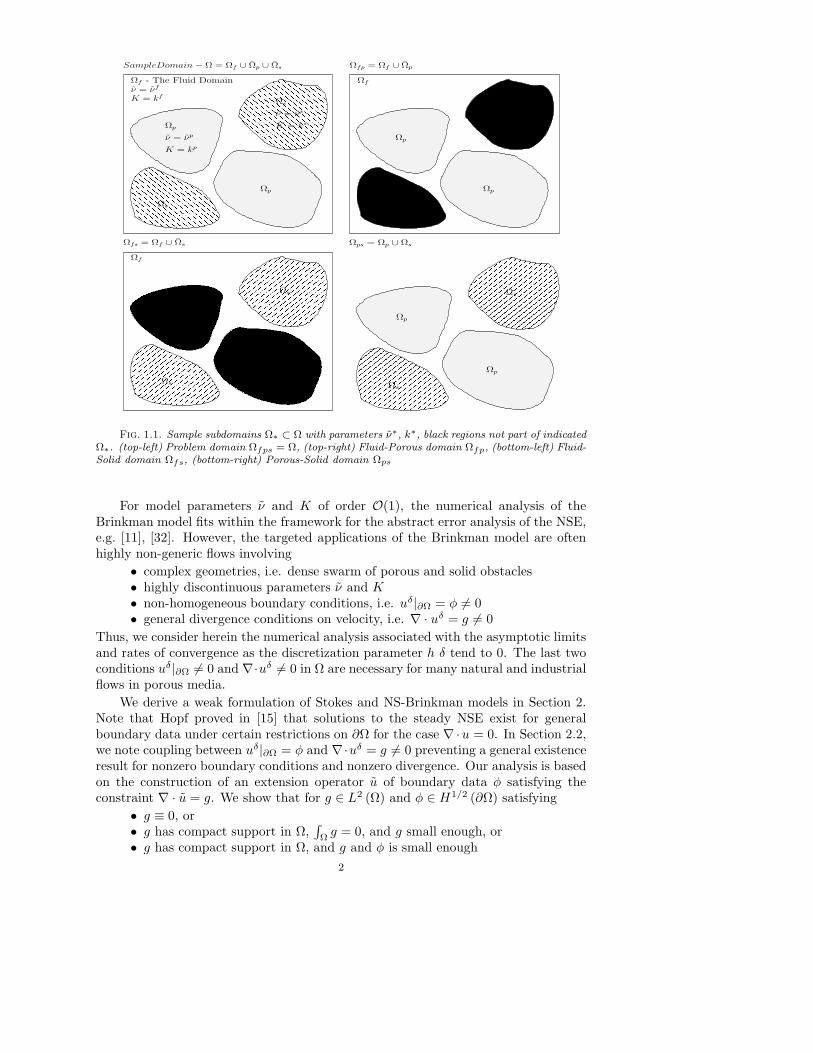
Experiment 2: Now we consider Ω = [0, 2] × [0, 1], ν = 10−2, νs = 1/δ, Kf =1/δ, Ks = δ. Here, we consider a 0.2×0.2 source g = 1 centered in the domain Ω andthe resulting flow around two square obstacles as shown in Figure 4.1 with imposedDirichlet boundary conditions
Fig. 4.1. Experiment 2: (top) problem domain, dark squares represent solid obstacles, (bottom)NS-Brinkman velocity approximation
u|x=0 = −0.12y(1− y), u|x=2 = 0.12y(1− y), uy=0,1 = 0
A uniform triangular mesh is used. The velocity plot in Figure 4.1 shows theNS-Brinkman approximation to the proposed flow for Experiment 2 correspondingwith our intuition. To quantify the accuracy of the approximation, we list the L2
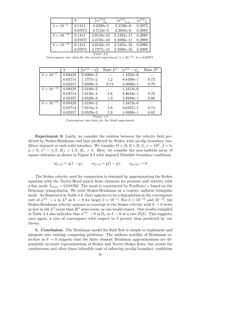
norm of uδ,h in Ωs and H1 semi-norm in Ωs and Ω for several combinations of h andδ-values in Table 4.2. Notice that
∥∥uδ,h
∥∥ and
∣∣uδ,h
∣∣1,s
converge at a rate O(δ) for
each indicated h. This is better than the O(√δ) suggested by our theory. Also note
that∣∣uδ,h
∣∣1
remains bounded (relatively constant in fact) with h and δ.
27
h∥∥uδ,h
∥∥
s
∣∣uδ,h
∣∣1,s
∣∣uδ,h
∣∣1
δ = 10−5 0.1414 4.6299e-5 2.1236e-6 0.29730.07071 4.7124e-5 2.3095e-6 0.2992
δ = 10−10 0.1414 4.6543e-10 2.1334e-11 0.29800.07071 4.4738e-10 2.3206e-11 0.2999
δ = 10−15 0.1414 4.6543e-15 2.1335e-16 0.29800.07071 4.7377e-15 2.3296e-16 0.2999
Table 4.2
Convergence rate data for the second experiment; δ = 10−15, h = 0.07071
h∥∥uδ,h − u
∥∥ Rate L2
∣∣uδ,h − u
∣∣1
Rate H1
δ = 10−5 0.09428 2.6968e-2 — 1.4324e-0 —0.04714 1.1757e-2 1.2 8.6499e-1 0.730.02357 7.0509e-3 0.74 4.9880e-1 0.79
δ = 10−10 0.09428 2.4180e-2 — 1.4413e-0 —0.04714 7.9136e-3 1.6 8.8644e-1 0.700.02357 2.0529e-3 1.9 4.8989e-1 0.86
δ = 10−15 0.09428 2.4180e-2 — 1.4413e-0 —0.04714 7.9154e-3 1.6 8.6437e-1 0.740.02357 2.0529e-3 1.9 4.8989e-1 0.82
Table 4.3
Convergence rate data for the third experiment
Experiment 3: Lastly, we consider the relation between the velocity field pre-dicted by Stokes-Brinkman and that predicted by Stokes with no-slip boundary con-dition imposed at each solid interface. We consider Ω = [0, 2]× [0, 1], ν = 102, f = 0,g = 0, νs = 1/δ, Kf = 1/δ, Ks = δ. Here, we consider the non-uniform array ofsquare obstacles as shown in Figure 4.2 with imposed Dirichlet boundary conditions
u|x=0 = y(1 − y), u|x=2 = y(1 − y), uy=0,1 = 0
The Stokes velocity used for comparison is obtained by approximating the Stokesequation with the Taylor-Hood mixed finite elements for pressure and velocity witha fine mesh, hmax = 0.018760. The mesh is constructed by FreeFem++ based on theDelaunay triangulation. We solve Stokes-Brinkman on a coarser, uniform triangularmesh. As illustrated in Table 4.3, there appears to be a degradation in the convergencerate of uδ,h → u in L2 as h → 0 for larger δ = 10−5. For δ = 10−10 and 10−15, theStokes-Brinkman velocity appears to converge to the Stokes velocity with h→ 0 twiceas fast in the L2 norm than H1 semi-norm, as one would expect. Our results compiledin Table 4.4 also indicates that uδ,h → 0 in Ωs as δ → 0 at a rate O(δ). This suggests,once again, a rate of convergence with respect to δ greater than predicted by ourtheory.
5. Conclusion. The Brinkman model for fluid flow is simple to implement andintegrate into existing computing platforms. The uniform stability of Brinkman ve-locities as δ → 0 suggests that the finite element Brinkman approximations are de-pendably accurate representations of Stokes and Navier-Stokes flows, but avoids thecumbersome and often times infeasible task of enforcing no-slip boundary conditions
28
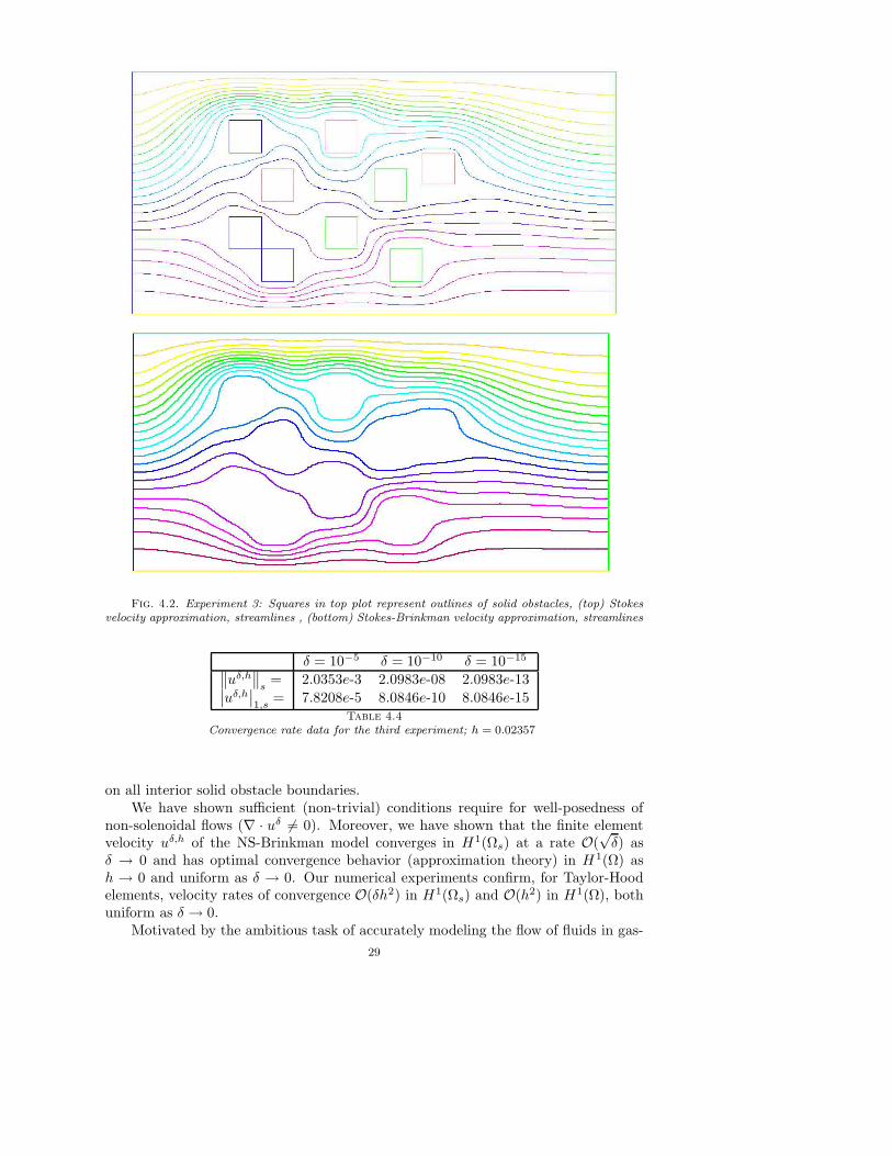
Fig. 4.2. Experiment 3: Squares in top plot represent outlines of solid obstacles, (top) Stokesvelocity approximation, streamlines , (bottom) Stokes-Brinkman velocity approximation, streamlines
δ = 10−5 δ = 10−10 δ = 10−15∥∥uδ,h
∥∥
s= 2.0353e-3 2.0983e-08 2.0983e-13
∣∣uδ,h
∣∣1,s
= 7.8208e-5 8.0846e-10 8.0846e-15Table 4.4
Convergence rate data for the third experiment; h = 0.02357
on all interior solid obstacle boundaries.We have shown sufficient (non-trivial) conditions require for well-posedness of
non-solenoidal flows (∇ · uδ 6= 0). Moreover, we have shown that the finite elementvelocity uδ,h of the NS-Brinkman model converges in H1(Ωs) at a rate O(
√δ) as
δ → 0 and has optimal convergence behavior (approximation theory) in H1(Ω) ash → 0 and uniform as δ → 0. Our numerical experiments confirm, for Taylor-Hoodelements, velocity rates of convergence O(δh2) in H1(Ωs) and O(h2) in H1(Ω), bothuniform as δ → 0.
Motivated by the ambitious task of accurately modeling the flow of fluids in gas-
29
cooled, pebble-bed nuclear reactors, we are interested in extending the Brinkmanmodel to the case of compressible fluids and coupling Brinkman flow with the equa-tions of convective and radiative heat transfer. Our preliminary finite element analysisfor the steady NS-Brinkman provides encouragement for these advances.
Acknowledgment Thank you, Prof. William Layton, for providing endlessideas, discussions, and encouragement.
REFERENCES
[1] G. Allaire, Homogenization of the navier-stokes equations in open sets perforated with tinyholes i. abstract framework, a volume distribution of holes, Arch. Ration. Mech. Anal., 113(1991), pp. 209–259.
[2] P. Angot, Analysis of singular perturbations on the brinkman problem for fictious domainmodels of viscous flows, Math. Methods Appl. Sci., 22 (1999), pp. 1395–1412.
[3] P. Angot, C.H. Bruneau, and P. Fabrie, A penalization method to take into account obsta-cles in incompressible viscous flows, Numer. Math., 81 (1999), pp. 497–520.
[4] G.S. Beavers and D.D. Joseph, Boundary conditions at a naturally permeable wall, J. FluidMech., 30 (1967), pp. 197–207.
[5] A. Bejan and D.A. Nield, Convection in Porous Media, no. 4, Springer, New York, third ed.,2006.
[6] H.C. Brinkman, A calculation of the viscous force exerted by a flowing fluid on a dense swarmof particles, Appl. Sci. Res., A1 (1947), pp. 27–34.
[7] , On the permeability of media consisting of closely packed porous particles, Appl. Sci.Res., A1 (1947), pp. 81–86.
[8] D.B. Das, Hydrodynamic modelling for groundwater flow through permeable reactive barriers,Hydrological Processes, 16 (2002), pp. 3393–3418.
[9] R.K. Dash, K.N. Mehta, and G. Jayaraman, Casson fluid flow in a pipe filled with a homo-geneous porous medium, Int. J. Engng. Sci., 34 (1996), pp. 1145–1156.
[10] G.P. Galdi, An Introduction to the Mathematical Theory of the Navier-Stokes Equations,vol. II, Springer-Verlag, New York, 1994.
[11] V. Girault and P.A. Raviart, Finite Element Methods for Navier-Stokes Equations,Springer-Verlag, Berlin, 1986.
[12] S. A. Grady, M. Y. Hussaini, and M. M Abdullah, Placement of wind turbines using geneticalgorithms, Renewable Energy, 30 (2005), pp. 259–270.
[13] V. Gurau, Hongtan Liu, and S. Kakac, Two-dimensional model for proton exchange mem-brane fuel cells, AIChE Journal, 44 (1988), pp. 2410–2422.
[14] M.H Hamdan, Single-phase flow through porous channels a review of flow models and channelentry conditions, Appl. Math. Comput., 62 (1994), pp. 203–222.
[15] E. Hopf, On non-linear partial differential equations, Lecture Series of the Symposium onPartial Differential Equations, (1955).
[16] U. Hornung, ed., Homogenization and Porous Media, vol. 6, Springer, Berlin, 1997.[17] O. Iliev and V. Laptev, On numerical simulation of flow through oil filters, Comput. Vis.
Sci., 6 (2004), pp. 139–146.[18] M. Kaviany, Principles of heat transfer in porous media, Springer-Verlag, New York, 1991.[19] N.K.-R. Kevlahan and J.M. Ghidaglia, Computation of turbulent flow past an array of
cylinders using a spectral method with brinkman penalization, Eur. J. Mech. B Fluids, 20(2001), pp. 333– 350.
[20] K. Khadra, S. Parneix, P. Angot, and J.-P. Caltagirone, Fictitious domain approach fornumerical modelling of navier-stokes equations, Internat. J. Numer. Methods Fluids, 34(2000), pp. 651–684.
[21] W.J. Layton, F. Schieweck, and I. Yotov, Coupling fluid flow with porous media flow,SIAM J. Numer. Anal., 40 (2003), pp. 2195–2218.
[22] Q. Liu Liu and O.V. Vasilyev, A brinkman penalization method for compressible flows incomplex geometries, Journal of Computational Physics, 227 (2007), pp. 946–966.
[23] W. Lu, C.Y. Zhao, and S.A. Tassou, Thermal analysis on metal-foam filled heat exchangers.part i: Metal-foam filled pipes, Int. J. Heat Mass Transfer, 49 (2006), pp. 2751–2761.
[24] G. Marmidis, S. Lazarou, and E. Pyrgioti, Optimal placement of wind turbines in a windpark using monte carlo simulation, Renewable Energy, 33 (2008), pp. 1455–1460.
[25] D.A. Nield, Alternative models of turbulence in a porous medium, and related matters, Journalof Fluids Engineering, 123 (2001), pp. 928–931.
30
[26] I. Pop and B. Derek, Convective Heat Transfer: Mathematical and Computational Modellingof Viscous Fluids and Porous Media, Pergamon, New York, first ed., 2001.
[27] C.H. Rycroft, G.S. Grest, Landry.. J.W., and M.Z. Bazant, Dynamics of random packingsin granular flow, Phys. Rev. E (3), 73 (2006), p. 051306.
[28] C.H. Rycroft, G.S. Grest, J.W. Landry, and M.Z. Bazant, Analysis of granular flow ina pebble-bed nuclear reactor, Phys. Rev. E (3), 74 (2006), p. 021306.
[29] P.G. Saffman, On the boundary condition at the surface of a porous medium, Stud. Appl.Math., L (1971), pp. 93–101.
[30] B. Straughan, Stability and Wave Motion in Porous Media: Applied Mathematical Sciences,Springer, New York, first ed., 2008.
[31] Shigeru Tada and J.M. Tarbell, Interstitial flow through the internal elastic lamina affectsshear stress on arterial smooth muscle cells, Am. J. Physiol Heart Circ. Physiol, 278 (2000),pp. H1589–H1597.
[32] R. Temam, Navier-Stokes Equations; Theory and Numerical Analysis, AMS, New York,fourth ed., 2001.
[33] X. Xie, J. Xu, and G. Xue, Uniformly-stable finite element methods for darcy-stokes-brinkmanmodels, J. Comp. Math., 26 (2008), pp. 437–455.
31
Recommended