Download pdf - A hierarchical clustering-based routing protocol for ... · PDF fileA hierarchical clustering-based routing ... hierarchical clustering-based routing protocol for wireless sensor

Int. J. Sensor Networks, Vol. 4, Nos. 1/2, 2008 79

Copyright © 2008 Inderscience Enterprises Ltd.

A hierarchical clustering-based routing protocol for wireless sensor networks supporting multiple data aggregation qualities

Yongyu Jia, Lian Zhao* and Bobby Ma Department of Electrical and Computer Engineering, Ryerson University, Toronto, Ontario, Canada E-mail: [email protected] E-mail: [email protected] E-mail: [email protected] *Corresponding author

Abstract: Wireless Sensor Networks (WSNs) consist of a large number of energy-limited sensor nodes that are densely deployed in a large geographical region. For WSNs, energy efficiency is always a key design issue to improve the life span of the network. In this paper, we propose a routing protocol, called the Clustering-Based Expanding–Ring Routing Protocol (CBERRP), which mainly focuses on the network layer while integrating factors from other layers to gain the preferred performance. CBERRP is a centralised scheme which is controlled by the Base Station (BS) and utilises the two-level hierarchical structure of clusters and chains to route the sensed data to the BS. In addition, CBERRP can be fine-tuned to support multiple Data Aggregation Qualities. The performance of CBERRP is compared to Low-Energy Adaptive Clustering Hierarchy (LEACH) and LEACH-Centralised (LEACH-C). Simulation results show that CBERRP presents significant improvement on power consumption, throughput and the network lifetime.

Keywords: energy balancing algorithm; hierarchical routing protocol; Wireless Sensor Networks; WSNs; simulation; Reference Point; RP.

Reference to this paper should be made as follows: Jia, Y., Zhao, L. and Ma, B. (2008) ‘A hierarchical clustering-based routing protocol for wireless sensor networks supporting multiple data aggregation qualities’, Int. J. Sensor Networks, Vol. 4, Nos. 1/2, pp.79–91.

Biographical notes: Yongyu Jia completed his BSc and MASc degrees at North-eastern University, China, in 1997 and at Ryerson University, Canada, in 2006, respectively. He has been working with BCSGlobal as a Senior Network Engineer since his graduation. His research interests are IP network and wireless network.

Dr. Lian Zhao is an Associate Professor at the Department of Electrical and Computer Engineering at Ryerson University, Toronto, Canada.

Dr. Bobby Ma is a Professor at the Department of Electrical and Computer Engineering at Ryerson University, Toronto, Canada.

1 Introduction

Owing to the advances in sensor technology, low-power electronics and wireless communication, Wireless Sensor Networks (WSNs) have become an indispensable and necessary tool to carry out many applications impossible for other types of networks (Akyildiz et al., 2002). Examples of these applications include tracking contamination in hazardous environments, habitat monitoring in the nature preserves, enemy tracking in battlefield environments, traffic monitoring, surveillance of buildings, etc. A typical sensor network has a great number of nodes, which are scattered over a region of interest. All the sensor nodes sense and gather information in a coordinated manner, and then pass the sensed information to the Base Station (BS)

over the path determined by the routing protocol. Since the sensor nodes are equipped with small, often irreplaceable batteries with limited power capacity, it is essential that the network be energy efficient in order to maximise the life span of the network (Akyildiz et al., 2002; Heinzelman et al., 2002).

Recently, power-aware WSNs design has attracted great research attention across different layers of the communication stack. For example, in Raghunathan et al. (2002), several factors affecting the power consumption in terms of characteristics of the radio, including the type of modulation scheme, data rate, transmit power (determined by the transmission distance) and the operational duty cycle are investigated. A Medium Access Control (MAC) protocol designed for WSNs, called S-MAC, is proposed in

80 Y. Jia, L. Zhao and B. Ma

Ye et al. (2002). S-MAC uses three novel techniques to reduce energy consumption and support self-configuration. First, to reduce energy consumption in listening to an idle channel, nodes periodically sleep. Second, neighbouring nodes form virtual clusters to auto-synchronise on sleep schedules. Third, S-MAC applies message passing to reduce contention latency for sensor-network applications that require store-and-forward processing as data move through the network. The characteristics of the power dissipation in MAC layer are also examined in Shih et al. (2001) and El-Hoiydi and Decotignie (2004). Although a few potential researches introduced in Akyildiz et al. (2002) are ongoing, the power-efficient protocols in transport and application layers remain a largely unexplored region. In contrast, the research of power-aware protocol in network layer shows a significant difference due to the close connection between power consumption and the routing scheme when the ‘power metric’ is taken into account to select the best path in the network, for example, the Energy Efficient Routing in Schurgers and Srivastava (2001).

A comprehensive survey of the routing protocols for WSNs can be found in Jiang and Manivannan (2004). In general, these protocols can be categorised into two classes according to the node’s participating style: flat protocols and clustering protocols. Those in Hedetniemi and Liestman (1988), Heinzelman et al. (1999), Sohrabi et al. (2002) and Intanagonwiwat et al. (2000) belong to the first class, whereas the protocol in Heinzelman et al. (2002) belongs to the second class, i.e. Low-Energy Adaptive Clustering Hierarchy (LEACH), which is one of the most fundamental and elegant protocol frameworks in the literature. LEACH is a clustering-based protocol architecture utilises randomised rotation of the Cluster-Heads (CHs) to uniformly distribute the energy budget across the network. The sensor nodes are grouped into several clusters and in each cluster, one of the sensor nodes is selected to be CH. Each node will transmit its data to its own CH which forwards the sensed data to the BS finally. Both the communication between sensor nodes and CH and that between CHs and the BS are direct, single-hop transmission. Based on the framework of LEACH, several protocols are proposed in the open literature. In Lindsey et al. (2002), a scheme called Power-Efficient GAthering in Sensor Information System (PEGASIS) is proposed. In this system, each node communicates only with a close neighbour and takes turns transmitting to the BS, thus reducing the amount of energy spent per round. The greedy algorithm is used by sensor nodes to form a single chain in the WSN; the sensed data from each sensor is forwarded along with the chain to a designated node which in turn forwards the collected data to the BS. The designated node is called chain-leader which is chosen rotationally among all the sensor nodes in order to evenly dissipate power. It is obvious in PEGASIS that long latency and sophisticated synchronisation are still challenges to be addressed. Moreover, due to the rotation of chain-leaders, the scenario of data going back and forth before arriving at the BS cannot be avoided, and therefore, it is not power efficient. In Muruganathan et al. (2005), Base Station Controlled Dynamic Clustering Protocol (BCDCP)

utilises the BS to set up the clusters and routing paths. The key idea of BCDCP is in the setting-up phase, a cluster split algorithm is applied to make each CH serves an approximately equal number of member nodes to avoid CH overload. It also applies Cluster-Head-to-Cluster-Head (CH-to-CH) routing to transfer the data to the BS. One shortcoming is that it cannot achieve the optimal number of clusters given the size of the network. Another shortcoming is that BCDCP cannot avoid the over utilisation of the near-to-BS sensor nodes when CH-to-CH routing protocol is used; thus power consumption on these nodes is more than that on those far-to-BS nodes, resulting an uneven power dissipation throughout the whole network. In Zhao et al. (2005), multi-hop routing is utilised for inter-cluster communication between CHs and the BS, instead of direct transmission, in order to minimise transmission energy. The shortcoming is that the closer-to-BS nodes will drain their power earlier than the further away nodes due to increased forwarding to the remote BS. The complexity of the global iterative algorithm to find the minimum sum square distance path is not encouraging.

In this paper, we also focus on the design of power efficient network layer solutions. Our work is inspired by the previous approaches, but it differs by designing the protocol with the integration of the cross-layer design principle which is proven to be a pertinent method to meet the challenges of power-constrained WSNs or Mobile Ad hoc NETworks (MANETs) (Goldsmith and Wicker, 2002). A novel clustering-based routing protocol called Clustering-Based Expanding–Ring Routing Protocol (CBERRP) is proposed in this paper to improve the effective lifetime of the WSNs with a limited energy supply. The salient feature of the proposed algorithm over previous LEACH-based algorithms include: (i) the node that is closer to the centre of a cluster has a higher priority to become the CH of the cluster, making the power consumption within Level-I cluster minimum. This is based on the fact (proof provided in Section 3.1) that for a uniformly distributed sensor cluster, the expected sum of the energy consumption is minimised when the CH locates at the centre of the cluster; (ii) unlike in Muruganathan et al. (2005), the number of clusters in CBERRP is able to follow the optimal solution for the number of clusters provided in Heinzelman et al. (2002); (iii) CBERRP is a two-level-hierarchy clustering-based routing protocol. The proposed CBERRP runs in the high-energy BS to set up clusters and chain-like paths among the CHs to deliver the sensed data to the BS. After the formation of the clusters, CBERRP groups the CHs into Level-II clusters based on the rings that are concentric circles with the BS as the centre. These rings look like a rainbow from the viewpoint of BS. Within each ring (a colour arch in the rainbow), the CHs form a chain, and then one of the CHs in the chain will be predetermined as the chain-leader which is designated to transmit the aggregated data to the BS on behalf of the entire chain. The CH chain, which is a new and upper level cluster introduced in CBERRP, is composed of a set of CHs, instead of normal sensor nodes. The chain is formed based on the distance

A hierarchical clustering-based routing protocol for WSNs 81

from CH to the BS, i.e. the formation of the chains is in accordance with the rings that are concentric circles to the BS. Thus, compared with Lindsey et al. (2002), CBERRP alleviates ‘round trip’ data path from a closer-to-BS CH to a further-away CH when the chain-leader is rotated to the further-away CH.

The remainder of this paper is organised as follows. Section 2 presents the network and radio models adopted in CBERRP. A detailed description of CBERRP is then presented in Section 3. Sections 4 and 5 give our analysis of CBERRP and the simulation results, respectively. Finally, Section 6 concludes the paper.

2 System model

2.1 Network model and architecture

One typical application of the WSNs is the monitoring of a remote environment. Since the data sensed by one node is often highly correlated with that from other nearby nodes, the BS does not require all the (redundant) data; rather, the BS needs a high-level function of the data that describes the events occurring in the monitoring environment (Heinzelman et al., 2002). The clustering infrastructure takes advantage of this data aggregation (or data fusion) of the correlated data into a smaller set of messages that maintains the effective information for transmission. In the following, we describe the assumed properties of the wireless sensor node and the underlying network model studied in this work.

The studied WSN is homogenous, where all sensor nodes are identical in terms of functionality and structure. The BS is located far away from the sensor nodes. The sensor nodes are energy constrained with the same initial energy allocation. The nodes are equipped with power control capabilities to vary their transmitting power. Each node senses the environment at a fixed rate and always has data sent to the BS. All sensor nodes are dual-stack in modulation, supporting both Time Division Multiple Access (TDMA) and Code Division Multiple Access (CDMA). The location information of the nodes is known at the BS. The transmission of MAC layer is reliable.

It is clear that there are two key components in the underlying WSN model: the sensor node and the BS. The sensor nodes are geographically grouped into clusters and capable of operating in two basic modes: the CH mode and the sensor mode. In the sensor mode, the nodes perform sensing tasks and transmit the sensed data to the CH. In CH mode, a node gathers data from other sensing nodes within its cluster, performs data fusion and routes the data to the BS directly or through other CH nodes, if needed. The BS finally processes the received data and passes them to the end user through other means of communications, for example, the wired networks or satellite communication. In addition to data processing and transmission, the BS in CBERRP also serves as a central controller to perform the key tasks of CBERRP including cluster formation,

randomised CH selection and chains formation among all the CHs.

2.2 Radio model

A typical sensor node consists of four major components: (i) a data processor unit; (ii) a micro-sensor; (iii) a radio communication subsystem that consists of transmitter/ receiver electronics, antenna and an amplifier; and (iv) a power supply unit. Although energy is dissipated in all of the first three components of a sensor node, we mainly consider the energy dissipations associated with the radio component since the core objective of this paper is to develop an energy-efficient network layer protocol to improve the power conservation of the whole WSN occurring in data transmission. In addition, energy dissipated during data aggregation in the CH nodes is also taken into account.

In order to evaluate the energy dissipation, we accept the same radio model used in Heinzelman et al. (2002) and Muruganathan et al. (2005). The transmit and receive energy costs for the transfer of a k-bit data message between two nodes separated by r metres are given by

amp( , ) ( )T TxE k r E k E r k= + (1)

( )R RxE k E k= (2)

where ( , )TE k r in equation (1) denotes the total energy dissipated in the transmitter of the source node, and ( )RE k in equation (2) represents the energy cost incurred in the receiver. The parameters ETx and ERx in equation (1) and equation (2) are the per bit energy dissipations for transmission and reception, respectively. Eamp(r) is the energy required by the transmit amplifier to maintain an acceptable Signal-to-Interference-Noise Ratio (SINR) in order to transfer data messages reliably. Similarly in Heinzelman et al. (2002) and Muruganathan et al. (2005), we use both the free-space propagation model and the two-ray ground propagation model to approximate the path loss occurred in data transmission. Given a threshold transmission distance of r0, the free-space model is employed when 0 ,r r≤ and the multi-path model is applied when 0r r> . Using these two models, the energy required by the transmit amplifier amp ( )E r is given by

2FS 0

4ampMP 0

( ) r r rE r r r rεε⎧ ≤= ⎨ >⎩

(3)

where FS MPandε ε denote transmit amplifier parameters corresponding to the free-space and the multi-path models, respectively, and r0 is the threshold distance given by

FS0

MP

.rεε

= (4)

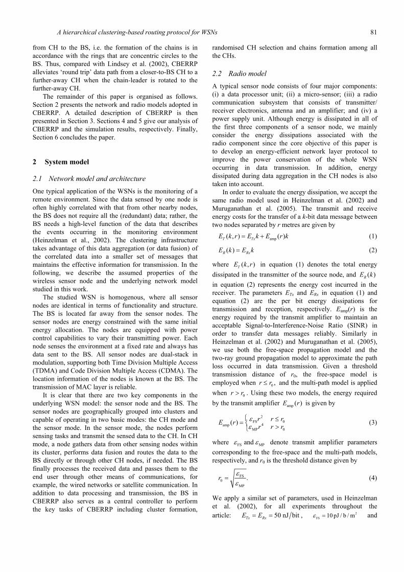
We apply a similar set of parameters, used in Heinzelman et al. (2002), for all experiments throughout the article: 50 nJ bitTx RxE E= = , 2

FS 10 pJ / b / mε = and


4MP 0.0013 pJ / b / mε = . Moreover, the energy cost for data

aggregation is set as DA 5 nJ / b / messageE = and all sensor nodes are deployed with an initial energy of 2J.

Furthermore, CBERRP classifies the communications in the WSN into three classes: (i) Level-I cluster communication is between sensor nodes and CH; (ii) Level-II cluster communication is between CHs in the same chain. These two classes of communications can also be referred to as short- and medium-distance communications; and (iii) long-distance communication is between the chain-leader and the BS. Note that data communications in the Level-I clusters are direct, while data communications in the Level-II clusters are hop-by-hop among the CHs with the chain-leader as the destination. Unlike other approaches, the integration of single-hop and multi-hop routing in CBERRP reaps the benefits from the two mechanisms. Single-hop routing is used for short-distance communication in the Level-I cluster to avoid the collision and the long latency; while multi-hop routing is suited to the medium-distance communication where power consumption is significant if the single-hop routing is used.

Communication utilising the CDMA modulation technique in a cluster needs to address the radio interference caused by the transmission in the neighbouring clusters (Heinzelman et al., 2002). In CBERRP, each cluster is assigned a spreading code to distinguish the data transmissions inside the home cluster from the transmission in other clusters. Furthermore, once the data gathering process is complete, the CH uses another spreading code dedicated to the chain to forward data to the chain-leader or the BS. In addition, TDMA is incorporated with CDMA to avoid transmission collision within a cluster and the chain. The schedules of the time slots in TDMA are determined at the BS.

3 Clustering-based expanding–ring routing protocol

The CBERRP is a hierarchical WSN routing protocol which utilises BS as a central controller to perform most of the control tasks. Therefore, there is no need for sensor nodes to exchange the fancy routing protocol messages, making CBERRP very less workload and energy efficient. CBERRP operates in two major phases: initialisation phase and data transmission phase. The second phase is further divided into the set-up subphase and the data delivery subphase. In this section, we describe the details of these phases.

Before going into the details of CBERRP, we introduce some terms used in the operation of CBERRP as listed below.

1 Cluster: In general, a cluster is a group of objects with similar attributes. The cluster in this work is a group of sensor nodes classified into the same category with respect to the geography, that is, the distance of the sensor node away from the CHs.

2 Cluster head: It is a sensor node which not only senses the phenomena, but also collects the data from other

members of its home cluster and performs data aggregation. Note that each sensor node takes turn to be CH in order to evenly distribute power dissipation throughout the whole sensor network.

3 Ring: It is a term which describes the virtual topology of sensor field. Each ring is an arch strip which is the part, covering the sensor field, of the concentric circle with BS as centre.

4 Chain: It is used to describe the topology formed by the CHs. All the CHs within the same ring will form a chain, thus, the number of rings determines the number of chains in CBERRP. Chain can be considered as the second level cluster.

5 Chain-leader: It is a designated CH responsible for delivering the data back to the BS on behalf of the entire chain. Thus, the chain-leader collects the data not only from its home cluster, but also from other CHs of its home chain. Similar to the fact that each sensor node has chance to be a CH, each CH has chance to be a chain-leader.

6 Data fusion: This term and data aggregation are interchangeably used in this work. The techniques of data aggregation are used to combine several correlated data signals into a smaller set of information that maintains the effective data (i.e. the information content) of the original signals (Pham et al., 2004). For example, K data packets generated from K sensor nodes in one cluster will be aggregated into one packet by the appropriate CH.

7 Round: The whole lifetime of WSN in CBERRP is divided into rounds, and one round is equivalent to a period of time. The duration of one round is determined by the end user, for example, it is 20 s in our work. In this sense, the number of rounds the WSN lasts indicates the lifetime of the WSN. Meanwhile, it is exactly the round operation that makes the rotation of the CHs and chain-leaders possible since each time a round finishes, a new set of CHs and a new set of chain-leaders will be selected for the upcoming new round. Therefore, the power dissipation in the whole life of the WSN is distributed evenly among all the sensor nodes.

8 Frame: This term describes the format in the time domain of the data that is transferred in the wireless channel. Frame is composed of TDMA slots and is the basic component of the Round. The TDMA time slots are assigned for communications for each sensor node in the cluster and each CH in the chain. Within each frame, a sensor node has a designated slot for transmitting data to its CH. In addition, each CH in the chain is also assigned one time slot for transmitting the aggregated data of its cluster to the chain-leader. Thus, at the end of one frame, the BS will receive an aggregated packet from each of the CH. The number of frames that can be transmitted in one round, Nf, is


determined by three factors: the number of bits in a frame (Bf), the duration of the round (Tr) and the wireless channel bandwidth (BW), and is given by the following equation:

rf

f

BW.

TN

B⋅

= (5)

Note that the number of bits in a frame is the product of the length of the packet (Lp) and the number of time slots in the frame (Ns). Equation (5) can be rewritten as

rf

p s

BW.

TN

L N⋅

=⋅

(6)

Figure 1 shows the frame structure in the operation of CBERRP corresponding to the time line.

9 Wireless channel bandwidth: This term can also be called the fundamental capacity of a wireless channel. It dictates the maximum data rate that can be transmitted over the channel with arbitrarily small probability of error.

Figure 1 Frame structure in CBERRP

3.1 Initialisation phase

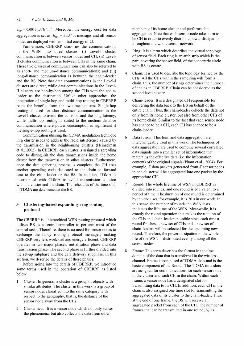
The initialisation phase accomplishes three activities. The first step in this phase is to partition the sensing area of WSN into a number of rings which are concentric circles with the BS as the centre. These rings are the basis where the chains are constructed. The second activity is to calculate the optimal number of the Level-I clusters, given both the region and the number of sensor nodes in the WSN. In Heinzelman et al. (2002), a formula is derived to calculate the optimum number of the clusters, given that N sensor nodes are randomly distributed in a K × K region, to minimise the energy dissipation. CBERRP will form a hierarchical topology of the WSN resulting from the combination of clusters and chains. After this, the whole sensor region obtains a logical grid view of the network topology, each grid is a cluster. For example, Figure 2 illustrates a WSN’s topology with six clusters and two rings.

The CBERRP will then calculate the location of the centre point for each grid. This location is referred to as a Reference Point (RP). The RP will be used in the data transmission phase for CH selection. It is always a challenge issue for the clustering-based algorithm to find an optimal

subset of nodes to be CHs in terms of power conservation. Many schemes proposed in the literature so far have tried to address this problem. In Heinzelman et al. (2002), the simulated annealing algorithm to solve the NP-hard problem of finding k optimal clusters is used. Other schemes choose the CHs or chain-leaders based on other considerations rather than the power consumption such as the random probability in Lindsey et al. (2002) and load-balance in Muruganathan et al. (2005). However, these schemes are either too complicated or suboptimal in terms of power consumption. By using the clustering architecture, CBERRP can utilise the cluster formation to minimise the power dissipation in the WSN. Thus, how to form the cluster becomes a key issue. Ideally, we hope that the shape of the clusters is as regular as possible, the distribution of the CHs is as even as possible and the sum of power consumption during the data communications is as small as possible. It is encouraging that the schemes with the help of the RP can meet these challenges desirably with very little computation.

Figure 2 An example of ring topology in CBERRP

By choosing the centre of each grid as the RP, we gain two advantages. First, it is obvious that using RPs can make the distribution of the CHs as uniform as possible throughout the whole WSN. Second, taking the centre of the grid as the RP makes the expectation of the sum of the square distance between sensor nodes and CH minimum. Since this sum is approximately proportional to the energy consumption required for the communications among sensing nodes and the CH (Heinzelman et al., 2002), the power consumption during the communication of the Level-I cluster will reach the minimum value. We prove this as following.

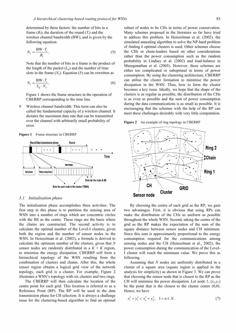
Assuming that N nodes are uniformly distributed in a cluster of a square area (square region is applied in the analysis for simplicity) as shown in Figure 3. We can prove that choosing the sensor node that is closest to the RP as the CH will minimise the power dissipation. Let node 1, (x1,y1) be the point that is the closest to the cluster centre (0,0). Hence, we have

2 2 2 21 1 , 1 .n nx y x y n N+ < + < ≤ (7)


Figure 3 A generic cluster (see online version for colours)

The expectation of the sum square distance between the ith nodes (i = 2,…,N) and the 1st node is:

( ) ( )2 21 1 1

2.

N

i ii

S E x x y y=

⎡ ⎤⎡ ⎤= − + −⎢ ⎥⎣ ⎦⎣ ⎦∑ (8)

Now we randomly choose a node besides the 1st node, namely node n (n ≠ 1), with coordinates ( , )n nx y , as the CH. The expectation of the sum square distance is given as

2 2

1,( ) ( ) .

N

n i n i ni i n

S E x x y y= ≠

⎡ ⎤= − + −⎢ ⎥

⎣ ⎦∑ (9)

By manipulating equation (8) and equation (9) with the fact E[X] = 0 and E[Y] = 0, we have following two equations, respectively:

( ) ( ) ( )2 2 2 21 1 1

21 ,

N

i ii

S E x y N E x y=

= + + − +∑ (10)

( ) ( ) ( )2 2 2 2

1,

1 .N

n i i n ni i n

S E x y N E x y= ≠

= + + − +∑ (11)

And then one step further:

( ) ( ) ( )2 2 2 21 1 1

12 ,

N

i ii

S E x y N E x y=

= + + − +∑ (12)

( ) ( ) ( )2 2 2 2

12 .

N

n i i n ni

S E x y N E x y=

= + + − +∑ (13)

Based on the prerequisite of equation (7), we can readily have

1 , 1 .nS S n N< < ≤ (14)

As a result, the RP can be thought as the preferred location of the CH for each cluster. This approach is also applied to the case that the sensor node is exactly located at the RP. Thus, the centre point of the grid is always an ideal RP for the CH. Moreover, the formation of the clusters is determined by the locations of the RPs by using this method, resulting in another important feature of the cross-layer design in CBERRP: the integration of the physical topology and cluster formation. This feature enhances

the performance of CBERRP when the topology is well engineered (more analysis will be given in ‘Simulation Results’ section).

With these necessary topology information, CBERRP is able to assign each sensor node in WSN into appropriate cluster and data communication schedules, which is done in data transmission phase.

3.2 Data transmission phase

The operation of data transmission phase in CBERRP is divided into rounds. Each round begins with a set-up subphase where the clusters and chains are organised and the schedules for data transmissions are created, followed by a data delivery subphase where data are transferred from the sensor nodes to the CH, then hopped to the chain-leader and to the BS.

3.2.1 Set-up subphase

The main tasks in the set-up subphase are CH selection, chain formation and schedule creation. At the beginning of the set-up subphase, the BS receives information on the current energy status and location information from all the nodes in the WSN. At the very beginning, since the energy level of each node is at the initial value, there is no need for sensor nodes to send energy information. From the first round on, the sensor nodes will send energy information to the BS by piggyback the energy information in the last packet of each round. Only nodes with the energy high enough to communicate directly with the BS and have not been CH in the previous rounds can be the candidate for the CH selection of this round. In order to ensure that all sensor nodes are CHs the same number of times, a flag is given to each sensor node to mark whether it has been CH once before. When all the sensor nodes have been the CHs once, these flags will be reset and the process of CH selection continues. This strategy keeps the random rotation of the CHs throughout the WSN to achieve even power dissipation among all the sensor nodes.

The CH selection in CBERRP is based on the following sorting and searching algorithm. The BS sorts all the sensor nodes based on the distance from each sensor node to those RPs obtained in the initialisation phase. The sensor node nearest to each RP of a cluster is preferred as the CH in the cluster. If the nearest sensor node either has been the CH in the previous rounds or without sufficient power, then the second nearest one to the RP in the same cluster is selected. The procedure continues on until a qualified sensor node is found. Based on the above description, it is clear that as the time passes by, the CHs change round by round. Consequently, the formation of Level-I clusters also changes. Hence, the cluster associations which indicate the membership between a certain CH and a certain sensor node change as well. Meanwhile, as the CH moves away from the nearest node to the RP, the power consumption within the cluster will no longer be minimal. However, this more energy cost trades off the fairness of the power dissipation among all sensor nodes in the cluster. As a result, the


power is evenly distributed throughout the whole network to prolong the lifetime of the WSN in the long run. Apparently, CBERRP has such a character as following. The RPs and rings are fixed for a certain initialisation setup. As the time passes by, the CHs change round by round. Consequently, the Level-I clusters also change the cluster associations, which are the membership between a certain CH and a certain sensor node.

After the selection of the CHs, the BS forms the chains following the rule that the CHs in the same chain must fall in the same ring. The selection of the chain-leader is based on the locations of the CHs. Specifically, the CH with the smallest distance to the BS is selected as the chain-leader. This chain-leader selection achieves the minimum power consumption in data delivery subphase without the loss of the feature of the random rotation of chain-leaders. It is clear that taking the CH closest to the BS in the chain as the chain-leader makes the sum of the squared distance minimal in the Level-II cluster. Meanwhile, the location of this CH is random, either. In other words, each CH may be closer to the BS than others in the same chain, which guarantees the randomness of the chain-leaders’ selection. This randomness achieves the evenly power dissipation among the clusters. It is this feature that makes CBERRP attractive since many other proposed routing protocols in the literature are not able to make a great balance between the rotation of the chain-leaders and the optimum of power dissipation.

The BS will advertise the resulting topology information including clusters’ formation, CHs and chains to all sensor nodes through broadcast. Thus, by letting the BS carry on most of the control tasks of the routing protocol, CBERRP minimises the energy consumption of running the routing protocol on all the sensor nodes. Along with the topology information broadcasted to the sensor nodes are the TDMA time slot schedules, one schedule for one cluster and the associated chain. Hence, each schedule specifies the slots used within each cluster and between CHs and the chain-leader. The sensor nodes deliver the sensed data to the BS in the data delivery subphase according to these schedules.

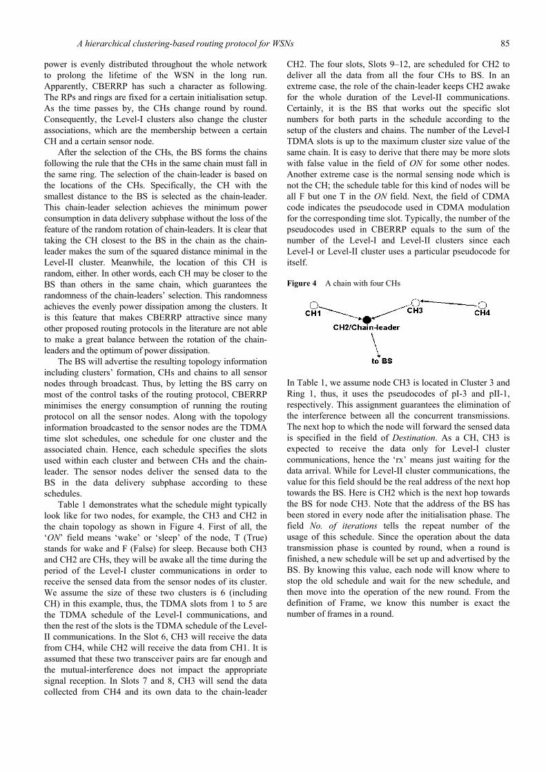
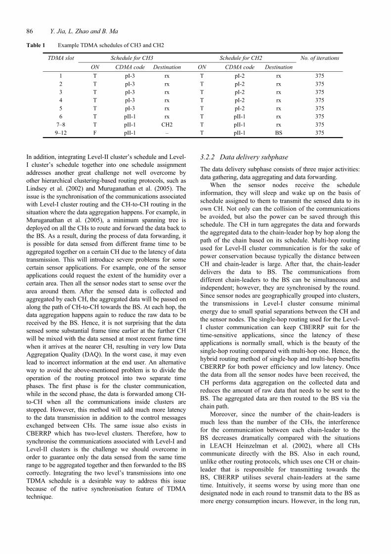
Table 1 demonstrates what the schedule might typically look like for two nodes, for example, the CH3 and CH2 in the chain topology as shown in Figure 4. First of all, the ‘ON’ field means ‘wake’ or ‘sleep’ of the node, T (True) stands for wake and F (False) for sleep. Because both CH3 and CH2 are CHs, they will be awake all the time during the period of the Level-I cluster communications in order to receive the sensed data from the sensor nodes of its cluster. We assume the size of these two clusters is 6 (including CH) in this example, thus, the TDMA slots from 1 to 5 are the TDMA schedule of the Level-I communications, and then the rest of the slots is the TDMA schedule of the Level-II communications. In the Slot 6, CH3 will receive the data from CH4, while CH2 will receive the data from CH1. It is assumed that these two transceiver pairs are far enough and the mutual-interference does not impact the appropriate signal reception. In Slots 7 and 8, CH3 will send the data collected from CH4 and its own data to the chain-leader

CH2. The four slots, Slots 9–12, are scheduled for CH2 to deliver all the data from all the four CHs to BS. In an extreme case, the role of the chain-leader keeps CH2 awake for the whole duration of the Level-II communications. Certainly, it is the BS that works out the specific slot numbers for both parts in the schedule according to the setup of the clusters and chains. The number of the Level-I TDMA slots is up to the maximum cluster size value of the same chain. It is easy to derive that there may be more slots with false value in the field of ON for some other nodes. Another extreme case is the normal sensing node which is not the CH; the schedule table for this kind of nodes will be all F but one T in the ON field. Next, the field of CDMA code indicates the pseudocode used in CDMA modulation for the corresponding time slot. Typically, the number of the pseudocodes used in CBERRP equals to the sum of the number of the Level-I and Level-II clusters since each Level-I or Level-II cluster uses a particular pseudocode for itself.

Figure 4 A chain with four CHs

In Table 1, we assume node CH3 is located in Cluster 3 and Ring 1, thus, it uses the pseudocodes of pI-3 and pII-1, respectively. This assignment guarantees the elimination of the interference between all the concurrent transmissions. The next hop to which the node will forward the sensed data is specified in the field of Destination. As a CH, CH3 is expected to receive the data only for Level-I cluster communications, hence the ‘rx’ means just waiting for the data arrival. While for Level-II cluster communications, the value for this field should be the real address of the next hop towards the BS. Here is CH2 which is the next hop towards the BS for node CH3. Note that the address of the BS has been stored in every node after the initialisation phase. The field No. of iterations tells the repeat number of the usage of this schedule. Since the operation about the data transmission phase is counted by round, when a round is finished, a new schedule will be set up and advertised by the BS. By knowing this value, each node will know where to stop the old schedule and wait for the new schedule, and then move into the operation of the new round. From the definition of Frame, we know this number is exact the number of frames in a round.


Table 1 Example TDMA schedules of CH3 and CH2

TDMA slot Schedule for CH3 Schedule for CH2 No. of iterations ON CDMA code Destination ON CDMA code Destination

1 T pI-3 rx T pI-2 rx 375 2 T pI-3 rx T pI-2 rx 375 3 T pI-3 rx T pI-2 rx 375 4 T pI-3 rx T pI-2 rx 375 5 T pI-3 rx T pI-2 rx 375 6 T pII-1 rx T pII-1 rx 375

7–8 T pII-1 CH2 T pII-1 rx 375 9–12 F pII-1 – T pII-1 BS 375

In addition, integrating Level-II cluster’s schedule and Level-I cluster’s schedule together into one schedule assignment addresses another great challenge not well overcome by other hierarchical clustering-based routing protocols, such as Lindsey et al. (2002) and Muruganathan et al. (2005). The issue is the synchronisation of the communications associated with Level-I cluster routing and the CH-to-CH routing in the situation where the data aggregation happens. For example, in Muruganathan et al. (2005), a minimum spanning tree is deployed on all the CHs to route and forward the data back to the BS. As a result, during the process of data forwarding, it is possible for data sensed from different frame time to be aggregated together on a certain CH due to the latency of data transmission. This will introduce severe problems for some certain sensor applications. For example, one of the sensor applications could request the extent of the humidity over a certain area. Then all the sensor nodes start to sense over the area around them. After the sensed data is collected and aggregated by each CH, the aggregated data will be passed on along the path of CH-to-CH towards the BS. At each hop, the data aggregation happens again to reduce the raw data to be received by the BS. Hence, it is not surprising that the data sensed some substantial frame time earlier at the further CH will be mixed with the data sensed at most recent frame time when it arrives at the nearer CH, resulting in very low Data Aggregation Quality (DAQ). In the worst case, it may even lead to incorrect information at the end user. An alternative way to avoid the above-mentioned problem is to divide the operation of the routing protocol into two separate time phases. The first phase is for the cluster communication, while in the second phase, the data is forwarded among CH-to-CH when all the communications inside clusters are stopped. However, this method will add much more latency to the data transmission in addition to the control messages exchanged between CHs. The same issue also exists in CBERRP which has two-level clusters. Therefore, how to synchronise the communications associated with Level-I and Level-II clusters is the challenge we should overcome in order to guarantee only the data sensed from the same time range to be aggregated together and then forwarded to the BS correctly. Integrating the two level’s transmissions into one TDMA schedule is a desirable way to address this issue because of the native synchronisation feature of TDMA technique.

3.2.2 Data delivery subphase

The data delivery subphase consists of three major activities: data gathering, data aggregating and data forwarding.

When the sensor nodes receive the schedule information, they will sleep and wake up on the basis of schedule assigned to them to transmit the sensed data to its own CH. Not only can the collision of the communications be avoided, but also the power can be saved through this schedule. The CH in turn aggregates the data and forwards the aggregated data to the chain-leader hop by hop along the path of the chain based on its schedule. Multi-hop routing used for Level-II cluster communication is for the sake of power conservation because typically the distance between CH and chain-leader is large. After that, the chain-leader delivers the data to BS. The communications from different chain-leaders to the BS can be simultaneous and independent; however, they are synchronised by the round. Since sensor nodes are geographically grouped into clusters, the transmissions in Level-I cluster consume minimal energy due to small spatial separations between the CH and the sensor nodes. The single-hop routing used for the Level-I cluster communication can keep CBERRP suit for the time-sensitive applications, since the latency of these applications is normally small, which is the beauty of the single-hop routing compared with multi-hop one. Hence, the hybrid routing method of single-hop and multi-hop benefits CBERRP for both power efficiency and low latency. Once the data from all the sensor nodes have been received, the CH performs data aggregation on the collected data and reduces the amount of raw data that needs to be sent to the BS. The aggregated data are then routed to the BS via the chain path.

Moreover, since the number of the chain-leaders is much less than the number of the CHs, the interference for the communication between each chain-leader to the BS decreases dramatically compared with the situations in LEACH Heinzelman et al. (2002), where all CHs communicate directly with the BS. Also in each round, unlike other routing protocols, which uses one CH or chain-leader that is responsible for transmitting towards the BS, CBERRP utilises several chain-leaders at the same time. Intuitively, it seems worse by using more than one designated node in each round to transmit data to the BS as more energy consumption incurs. However, in the long run,


the performance of the whole network will be improved by preventing all data load from converging at a single node in each round. Meanwhile, the latency can be decreased significantly by utilising multiple designated nodes compared with only one node utilised in each round, especially in a large scale WSN.

4 Discussion and analysis

Adopting the clustering architecture in the WSN provides many desirable properties. For example, with the clustering technology, the WSN is able to do the data aggregation and localised control. Clustering also provides a great scalability and self-configuration ability. However, only having clustering architecture is still not enough, many issues must be explored further to achieve the desired goals about the WSNs. Power efficiency is one of the most important aspects in the WSNs needed to be addressed. CBERRP is a scheme trying to meet some critical challenges arising from the WSN, such as limited energy consumption, routing issue and the quality of data aggregation, by following a cross-layer design concept at the very beginning. Typically, the cross-layer design indicates that information must be exchanged across all layers in the protocol stack. This information exchange allows the protocols to adapt in a global manner to the application requirements and underlying network conditions. In addition, all protocol layers must be jointly optimised with respect to global system constraints and characteristics. However, the way to fulfil the cross-layer design in traditional networks is not well suited for the WSN since a great deal of overhead will be generated by cross-layer mechanism and this overhead will degrade dramatically the performance of the WSN due to the limited resources of computation, memory and power on the tiny sensor. As a result, an alternative to a cross-layer design protocol is incorporating the factors from different layers into the operation of the proposed protocol. This method can eliminate the fancy overhead involved in the cross-layer design while retaining the benefits of it. Next, we would like to explore some properties, which have already been described in previous sections, in CBERRP in details.

The two-phase operation in CBERRP allows it to adapt to the change of DAQ introduced in Pham et al. (2004). Since DAQ varies proportionally with the number of clusters and inversely with the number of sensor nodes in each cluster, CBERRP can strike a balance between the optimal power consumption and the specific level of DAQ by manipulating the number of the rings. For example, DAQ of 12 clusters with four rings will be better than that of the same number of clusters with two rings, while in general, this benefit is obtained with the price of higher power consumption. Thus, CBERRP adapts to different DAQ requirements by setting up the appropriate number of rings in the initialisation phase in the following way: When the DAQ for the sensed data changes, a new initialisation phase is triggered after the current running round is finished. Furthermore, when the sensed data are passed along within

the chain, whether it is aggregated further or not can also be fine tuned, while without significantly affecting the power consumption.

It is clear that the requirement from the application layer such as DAQ can be met by manipulating the parameters in CBERRP, which shows the cross-layer design concept. The great scalability of CBERRP is also enhanced through the ring topology due to the fact that when the number of the rings is equal to or greater than the optimal number of the clusters, CBERRP in fact treats the WSN as a kind of topology like LEACH-C where each CH communicates directly to the BS; when the number of the rings decreases to 1, CBERRP converts the WSN to a kind of topology like C-PEGASIS in Pham et al. (2004) where all the CHs form a single chain, then only one of them as the chain-leader delivers the data signals to the BS. Thus, CBERRP can also be viewed as a general case for the above-mentioned two algorithms.

5 Simulation results

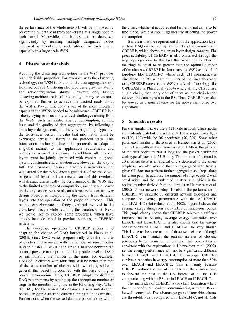
For our simulations, we use a 121-node network where nodes are randomly distributed in a 100 m × 100 m region from (0, 0) to (100, 100) with the BS coordinate (50, 200). Some other parameters similar to those used in Heinzelman et al. (2002) are the bandwidth of the channel is set to 1 Mbps, the payload of the data packet is 500 B long and the packet header for each type of packet is 25 B long. The duration of a round is 20 s, where there is an interval of 2 s dedicated to the set-up subphase. We also assume that the aggregated data from a given CH does not perform further aggregation as it hops along the chain path. In addition, the number of rings equals 2 with equal width and the number of clusters is 6 which is the optimal number derived from the formula in Heinzelman et al. (2002) for our network setup. To obtain the performance of CBERRP, we simulate 30 different network topologies and compare the average performance with that of LEACH and LEACH-C (Heinzelman et al., 2002). Figure 5 shows the average energy dissipation vs. number of simulation rounds. This graph clearly shows that CBERRP achieves significant improvement in reducing average energy dissipation over LEACH and LEACH-C. It is also shown that the energy consumptions of LEACH and LEACH-C are very similar. This is due to the same nature of these two schemes although LEACH-C can maintain the optimal number of clusters, producing better formation of clusters. This observation is consistent with the explanations in Heinzelman et al. (2002), i.e. the energy performance will not be significantly different between LEACH and LEACH-C. On average, CBERRP exhibits a reduction in energy consumption of more than 50% over LEACH and LEACH-C. This is mainly because CBERRP utilises a subset of the CHs, i.e. the chain-leaders, to forward the data to the BS, instead of all the CHs communicating with the BS like in LEACH and LEACH-C.

The main idea of CBERRP is the chain formation where the number of chain leaders communicating with the BS can be well controlled. The advantages gained from this scheme are threefold. First, compared with LEACH-C, not all CHs


communicate directly to the BS in each round resulting in less power consumption in the data delivery phase due to both fewer number of long distance (from CHs to the BS) transmissions and less interference coming from simultaneous communications between multiple CHs and the BS. Second, CBERRP decreases the average number of hops the data has to undergo before it arrives at the BS, compared to the algorithm which runs multi-hop routing protocol over all the CHs, such as, the algorithm in Zhao et al. (2005). Third, it is not surprising to see such a scenario in the WSN that the sensed data goes back and forth along the path in the course of delivering to the BS from the original sensing node. This is due to the suboptimal shortest path decision made by most of the WSN routing protocol, in which the power conservation is the single highest priority metric of interest. Moreover, the necessity of the rotation of CHs among all the sensor nodes does not allow us to always utilise the nearest node to the BS as the CHs, thus more power is ‘wasted’ on the way delivering the data to the BS, as the algorithms proposed in Lindsey et al. (2002) and Muruganathan et al. (2005). CBERRP remedies this in some extent by the ring architecture where the BS is the centre of each ring. That is, the maximum range that the sensed data can go back and forth is limited by the width of the ring; hence, the energy will be saved since the data coming from CH other than the chain-leader will not suffer a long round trip before it is forwarded to the BS through the chain-leader. This is exactly another beauty of the architecture of the rings. Therefore, in CBERRP, a perfect balance can be achieved for minimising the power consumption and keeping chain-leaders randomly rotating among all the CHs.

Figure 5 Energy dissipation

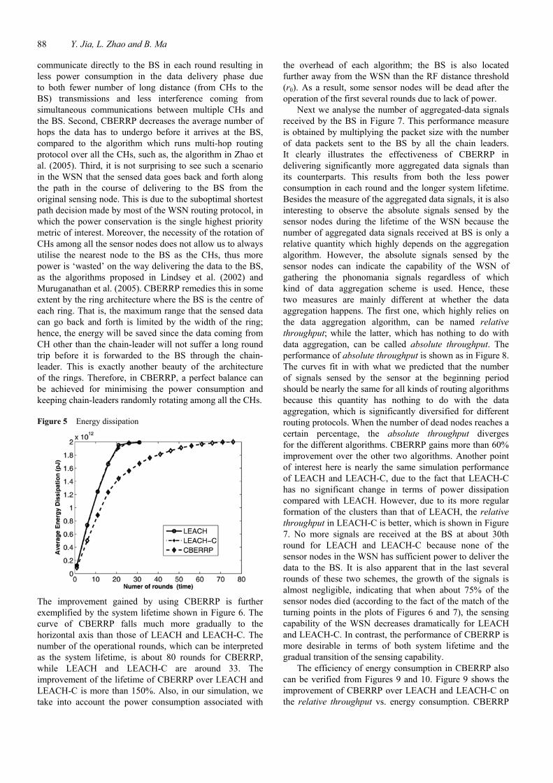
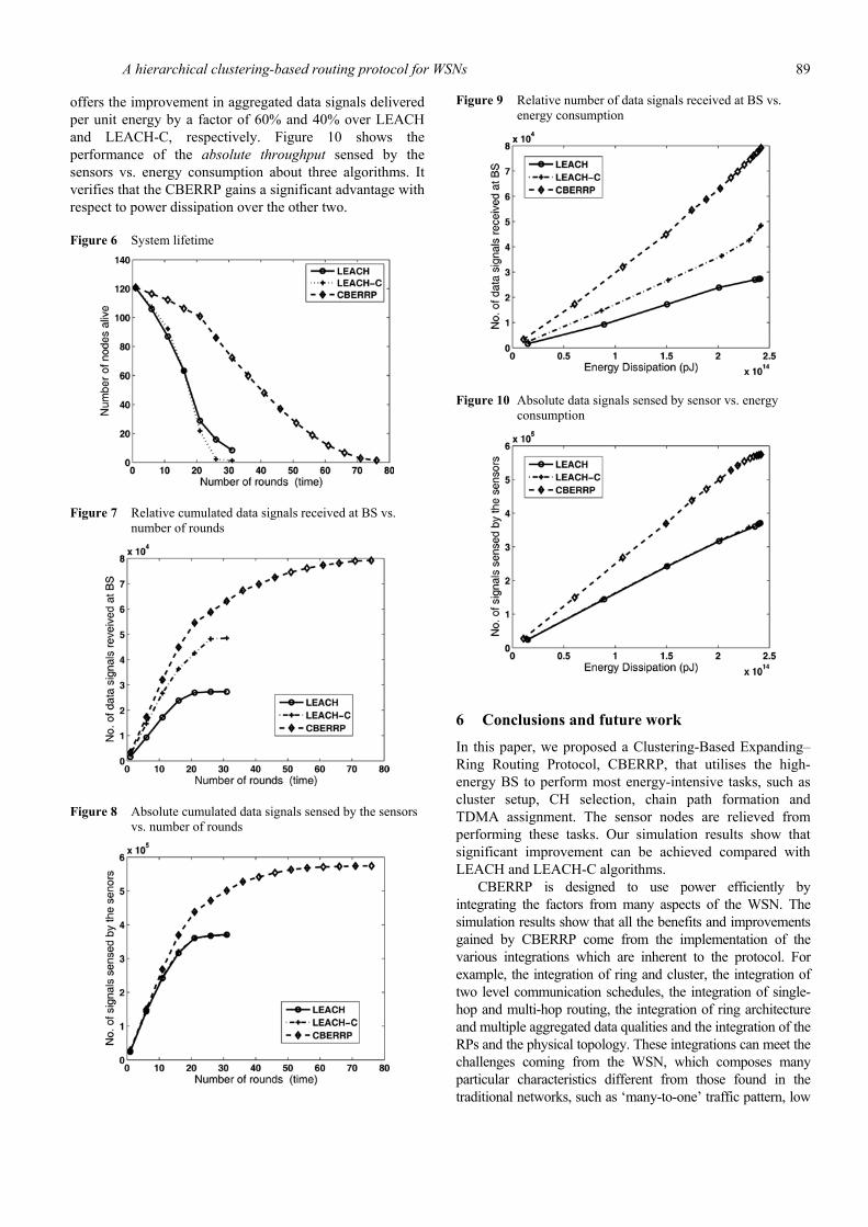
The improvement gained by using CBERRP is further exemplified by the system lifetime shown in Figure 6. The curve of CBERRP falls much more gradually to the horizontal axis than those of LEACH and LEACH-C. The number of the operational rounds, which can be interpreted as the system lifetime, is about 80 rounds for CBERRP, while LEACH and LEACH-C are around 33. The improvement of the lifetime of CBERRP over LEACH and LEACH-C is more than 150%. Also, in our simulation, we take into account the power consumption associated with

the overhead of each algorithm; the BS is also located further away from the WSN than the RF distance threshold (r0). As a result, some sensor nodes will be dead after the operation of the first several rounds due to lack of power.

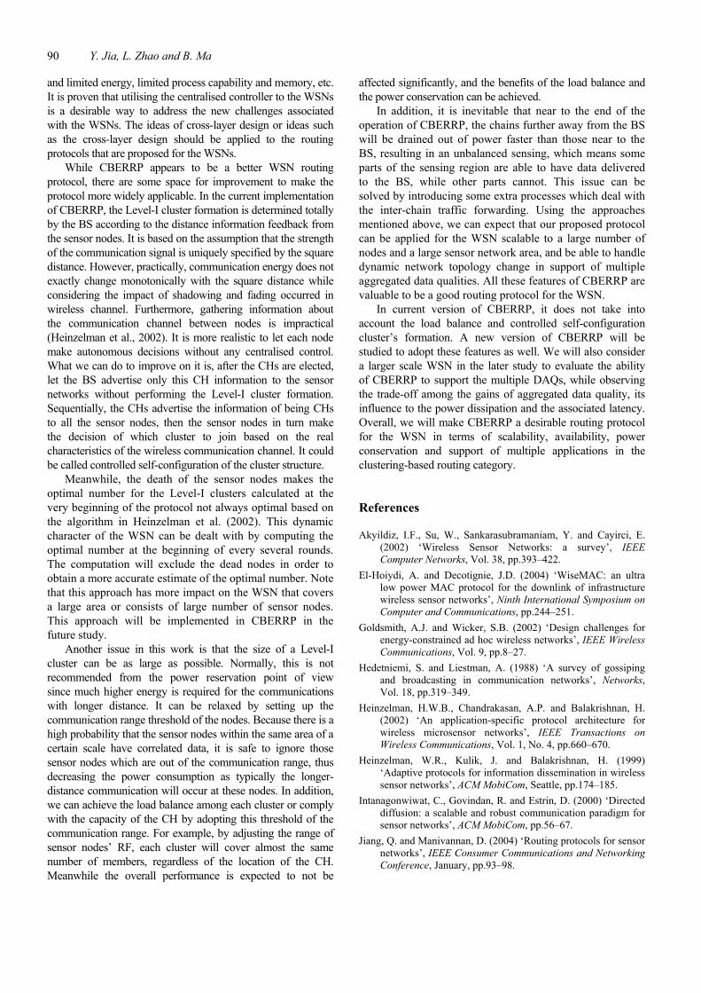
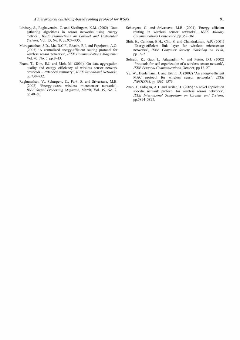
Next we analyse the number of aggregated-data signals received by the BS in Figure 7. This performance measure is obtained by multiplying the packet size with the number of data packets sent to the BS by all the chain leaders. It clearly illustrates the effectiveness of CBERRP in delivering significantly more aggregated data signals than its counterparts. This results from both the less power consumption in each round and the longer system lifetime. Besides the measure of the aggregated data signals, it is also interesting to observe the absolute signals sensed by the sensor nodes during the lifetime of the WSN because the number of aggregated data signals received at BS is only a relative quantity which highly depends on the aggregation algorithm. However, the absolute signals sensed by the sensor nodes can indicate the capability of the WSN of gathering the phonomania signals regardless of which kind of data aggregation scheme is used. Hence, these two measures are mainly different at whether the data aggregation happens. The first one, which highly relies on the data aggregation algorithm, can be named relative throughput; while the latter, which has nothing to do with data aggregation, can be called absolute throughput. The performance of absolute throughput is shown as in Figure 8. The curves fit in with what we predicted that the number of signals sensed by the sensor at the beginning period should be nearly the same for all kinds of routing algorithms because this quantity has nothing to do with the data aggregation, which is significantly diversified for different routing protocols. When the number of dead nodes reaches a certain percentage, the absolute throughput diverges for the different algorithms. CBERRP gains more than 60% improvement over the other two algorithms. Another point of interest here is nearly the same simulation performance of LEACH and LEACH-C, due to the fact that LEACH-C has no significant change in terms of power dissipation compared with LEACH. However, due to its more regular formation of the clusters than that of LEACH, the relative throughput in LEACH-C is better, which is shown in Figure 7. No more signals are received at the BS at about 30th round for LEACH and LEACH-C because none of the sensor nodes in the WSN has sufficient power to deliver the data to the BS. It is also apparent that in the last several rounds of these two schemes, the growth of the signals is almost negligible, indicating that when about 75% of the sensor nodes died (according to the fact of the match of the turning points in the plots of Figures 6 and 7), the sensing capability of the WSN decreases dramatically for LEACH and LEACH-C. In contrast, the performance of CBERRP is more desirable in terms of both system lifetime and the gradual transition of the sensing capability.

The efficiency of energy consumption in CBERRP also can be verified from Figures 9 and 10. Figure 9 shows the improvement of CBERRP over LEACH and LEACH-C on the relative throughput vs. energy consumption. CBERRP


offers the improvement in aggregated data signals delivered per unit energy by a factor of 60% and 40% over LEACH and LEACH-C, respectively. Figure 10 shows the performance of the absolute throughput sensed by the sensors vs. energy consumption about three algorithms. It verifies that the CBERRP gains a significant advantage with respect to power dissipation over the other two.

Figure 6 System lifetime

Figure 7 Relative cumulated data signals received at BS vs. number of rounds

Figure 8 Absolute cumulated data signals sensed by the sensors vs. number of rounds

Figure 9 Relative number of data signals received at BS vs. energy consumption

Figure 10 Absolute data signals sensed by sensor vs. energy consumption

6 Conclusions and future work

In this paper, we proposed a Clustering-Based Expanding–Ring Routing Protocol, CBERRP, that utilises the high-energy BS to perform most energy-intensive tasks, such as cluster setup, CH selection, chain path formation and TDMA assignment. The sensor nodes are relieved from performing these tasks. Our simulation results show that significant improvement can be achieved compared with LEACH and LEACH-C algorithms.

CBERRP is designed to use power efficiently by integrating the factors from many aspects of the WSN. The simulation results show that all the benefits and improvements gained by CBERRP come from the implementation of the various integrations which are inherent to the protocol. For example, the integration of ring and cluster, the integration of two level communication schedules, the integration of single-hop and multi-hop routing, the integration of ring architecture and multiple aggregated data qualities and the integration of the RPs and the physical topology. These integrations can meet the challenges coming from the WSN, which composes many particular characteristics different from those found in the traditional networks, such as ‘many-to-one’ traffic pattern, low


and limited energy, limited process capability and memory, etc. It is proven that utilising the centralised controller to the WSNs is a desirable way to address the new challenges associated with the WSNs. The ideas of cross-layer design or ideas such as the cross-layer design should be applied to the routing protocols that are proposed for the WSNs.

While CBERRP appears to be a better WSN routing protocol, there are some space for improvement to make the protocol more widely applicable. In the current implementation of CBERRP, the Level-I cluster formation is determined totally by the BS according to the distance information feedback from the sensor nodes. It is based on the assumption that the strength of the communication signal is uniquely specified by the square distance. However, practically, communication energy does not exactly change monotonically with the square distance while considering the impact of shadowing and fading occurred in wireless channel. Furthermore, gathering information about the communication channel between nodes is impractical (Heinzelman et al., 2002). It is more realistic to let each node make autonomous decisions without any centralised control. What we can do to improve on it is, after the CHs are elected, let the BS advertise only this CH information to the sensor networks without performing the Level-I cluster formation. Sequentially, the CHs advertise the information of being CHs to all the sensor nodes, then the sensor nodes in turn make the decision of which cluster to join based on the real characteristics of the wireless communication channel. It could be called controlled self-configuration of the cluster structure.

Meanwhile, the death of the sensor nodes makes the optimal number for the Level-I clusters calculated at the very beginning of the protocol not always optimal based on the algorithm in Heinzelman et al. (2002). This dynamic character of the WSN can be dealt with by computing the optimal number at the beginning of every several rounds. The computation will exclude the dead nodes in order to obtain a more accurate estimate of the optimal number. Note that this approach has more impact on the WSN that covers a large area or consists of large number of sensor nodes. This approach will be implemented in CBERRP in the future study.

Another issue in this work is that the size of a Level-I cluster can be as large as possible. Normally, this is not recommended from the power reservation point of view since much higher energy is required for the communications with longer distance. It can be relaxed by setting up the communication range threshold of the nodes. Because there is a high probability that the sensor nodes within the same area of a certain scale have correlated data, it is safe to ignore those sensor nodes which are out of the communication range, thus decreasing the power consumption as typically the longer-distance communication will occur at these nodes. In addition, we can achieve the load balance among each cluster or comply with the capacity of the CH by adopting this threshold of the communication range. For example, by adjusting the range of sensor nodes’ RF, each cluster will cover almost the same number of members, regardless of the location of the CH. Meanwhile the overall performance is expected to not be

affected significantly, and the benefits of the load balance and the power conservation can be achieved.

In addition, it is inevitable that near to the end of the operation of CBERRP, the chains further away from the BS will be drained out of power faster than those near to the BS, resulting in an unbalanced sensing, which means some parts of the sensing region are able to have data delivered to the BS, while other parts cannot. This issue can be solved by introducing some extra processes which deal with the inter-chain traffic forwarding. Using the approaches mentioned above, we can expect that our proposed protocol can be applied for the WSN scalable to a large number of nodes and a large sensor network area, and be able to handle dynamic network topology change in support of multiple aggregated data qualities. All these features of CBERRP are valuable to be a good routing protocol for the WSN.

In current version of CBERRP, it does not take into account the load balance and controlled self-configuration cluster’s formation. A new version of CBERRP will be studied to adopt these features as well. We will also consider a larger scale WSN in the later study to evaluate the ability of CBERRP to support the multiple DAQs, while observing the trade-off among the gains of aggregated data quality, its influence to the power dissipation and the associated latency. Overall, we will make CBERRP a desirable routing protocol for the WSN in terms of scalability, availability, power conservation and support of multiple applications in the clustering-based routing category.

References

Akyildiz, I.F., Su, W., Sankarasubramaniam, Y. and Cayirci, E. (2002) ‘Wireless Sensor Networks: a survey’, IEEE Computer Networks, Vol. 38, pp.393–422.

El-Hoiydi, A. and Decotignie, J.D. (2004) ‘WiseMAC: an ultra low power MAC protocol for the downlink of infrastructure wireless sensor networks’, Ninth International Symposium on Computer and Communications, pp.244–251.

Goldsmith, A.J. and Wicker, S.B. (2002) ‘Design challenges for energy-constrained ad hoc wireless networks’, IEEE Wireless Communications, Vol. 9, pp.8–27.

Hedetniemi, S. and Liestman, A. (1988) ‘A survey of gossiping and broadcasting in communication networks’, Networks, Vol. 18, pp.319–349.

Heinzelman, H.W.B., Chandrakasan, A.P. and Balakrishnan, H. (2002) ‘An application-specific protocol architecture for wireless microsensor networks’, IEEE Transactions on Wireless Communications, Vol. 1, No. 4, pp.660–670.

Heinzelman, W.R., Kulik, J. and Balakrishnan, H. (1999) ‘Adaptive protocols for information dissemination in wireless sensor networks’, ACM MobiCom, Seattle, pp.174–185.

Intanagonwiwat, C., Govindan, R. and Estrin, D. (2000) ‘Directed diffusion: a scalable and robust communication paradigm for sensor networks’, ACM MobiCom, pp.56–67.

Jiang, Q. and Manivannan, D. (2004) ‘Routing protocols for sensor networks’, IEEE Consumer Communications and Networking Conference, January, pp.93–98.


Lindsey, S., Raghavendra, C. and Sivalingam, K.M. (2002) ‘Data gathering algorithms in sensor networks using energy metrics’, IEEE Transactions on Parallel and Distributed Systems, Vol. 13, No. 9, pp.924–935.

Muruganathan, S.D., Ma, D.C.F., Bhasin, R.I. and Fapojuwo, A.O. (2005) ‘A centralized energy-efficient routing protocol for wireless sensor networks’, IEEE Communications Magazine, Vol. 43, No. 3, pp.8–13.

Pham, T., Kim, E.J. and Moh, M. (2004) ‘On data aggregation quality and energy efficiency of wireless sensor network protocols – extended summary’, IEEE Broadband Networks, pp.730–732.

Raghunathan, V., Schurgers, C., Park, S. and Srivastava, M.B. (2002) ‘Energy-aware wireless microsensor networks’, IEEE Signal Processing Magazine, March, Vol. 19, No. 2, pp.40–50.

Schurgers, C. and Srivastava, M.B. (2001) ‘Energy efficient routing in wireless sensor networks’, IEEE Military Communications Conference, pp.357–361.

Shih, E., Calhoun, B.H., Cho, S. and Chandrakasan, A.P. (2001) ‘Energy-efficient link layer for wireless microsensor networks’, IEEE Computer Society Workshop on VLSI, pp.16–21.

Sohrabi, K., Gao, J., Ailawadhi, V. and Pottie, D.J. (2002) ‘Protocols for self-organization of a wireless sensor network’, IEEE Personal Communications, October, pp.16–27.

Ye, W., Heidemann, J. and Estrin, D. (2002) ‘An energy-efficient MAC protocol for wireless sensor networks’, IEEE INFOCOM, pp.1567–1576.

Zhao, J., Erdogan, A.T. and Arslan, T. (2005) ‘A novel application specific network protocol for wireless sensor networks’, IEEE International Symposium on Circuits and Systems, pp.5894–5897.