379
13
Portfolio Optimization
13.1 Introduction Portfolio models are concerned with investment where there are typically two criteria: expected return
and risk. The investor wants the former to be high and the latter to be low. There is a variety of measures
of risk. The most popular measure of risk has been variance in return. Even though there are some
problems with it, we will first look at it very closely.
13.2 The Markowitz Mean/Variance Portfolio Model The portfolio model introduced by Markowitz (1959), see also Roy (1952), assumes an investor has
two considerations when constructing an investment portfolio: expected return and variance in return
(i.e., risk). Variance measures the variability in realized return around the expected return, giving equal
weight to realizations below the expected and above the expected return. The Markowitz model might
be mildly criticized in this regard because the typical investor is probably concerned only with
variability below the expected return, so-called downside risk. The Markowitz model requires two
major kinds of information: (1) the estimated expected return for each candidate investment and (2) the
covariance matrix of returns. The covariance matrix characterizes not only the individual variability of
the return on each investment, but also how each investment’s return tends to move with other
investments. We assume the reader is familiar with the concepts of variance and covariance as
described in most intermediate statistics texts. Part of the appeal of the Markowitz model is it can be
solved by efficient quadratic programming methods. Quadratic programming is the name applied to the
class of models in which the objective function is a quadratic function and the constraints are linear.
Thus, the objective function is allowed to have terms that are products of two variables such as x2 and
x y.
Quadratic programming is computationally appealing because the algorithms for linear programs can
be applied to quadratic programming with only modest modifications. Loosely speaking, the reason only
modest modification is required is the first derivative of a quadratic function is a linear function. Because
LINGO has a general nonlinear solver, the limitation to quadratic functions is helpful, but not crucial.

380 Chapter 13 Portfolio Optimization
13.2.1 Example We will use some publicly available data from Markowitz (1959). Eppen, Gould and Schmidt (1991)
use the same data. The following table shows the increase in price, including dividends, for three
stocks over a twelve-year period:
Growth in Year S&P500 ATT GMC USX
43 1.259 1.300 1.225 1.149
44 1.198 1.103 1.290 1.260
45 1.364 1.216 1.216 1.419
46 0.919 0.954 0.728 0.922
47 1.057 0.929 1.144 1.169
48 1.055 1.056 1.107 0.965
49 1.188 1.038 1.321 1.133
50 1.317 1.089 1.305 1.732
51 1.240 1.090 1.195 1.021
52 1.184 1.083 1.390 1.131
53 0.990 1.035 0.928 1.006
54 1.526 1.176 1.715 1.908
For reference later, we have also included the change each year in the Standard and Poor’s/S&P
500 stock index. To illustrate, in the first year, ATT appreciated in value by 30%. In the second year,
GMC appreciated in value by 29%. Based on the twelve years of data, we can use any standard
statistical package to calculate a covariance matrix for three stocks: ATT, GMC, and USX. The matrix
is:
ATT GMC USX
ATT 0.01080754 0.01240721 0.01307513
GMC 0.01240721 0.05839170 0.05542639
USX 0.01307513 0.05542639 0.09422681
From the same data, we estimate the expected return per year, including dividends, for ATT, GMC,
and USX as 0.0890833, 0.213667, and 0.234583, respectively.
The correlation matrix makes it more obvious how two random variables move together. The
correlation between two random variables equals the covariance between the two variables, divided by
the product of the standard deviations of the two random variables. For our three investments, the
correlation matrix is as follows:
ATT GMC USX
ATT 1.0
GMC 0.493895589 1.0
USX 0.409727718 0.747229121 1.0
The correlation can be between 1 and +1 with +1 being a high correlation between the two.
Notice GMC and USX are highly correlated. ATT tends to move with GMC and USX, but not nearly so
much as GMC moves with USX.

Portfolio Optimization Chapter 13 381
Let the symbols ATT, GMC, and USX represent the fraction of the portfolio devoted to each of the
three stocks. Suppose, we desire a 15% yearly return. The entire model can be written as:
MODEL:
!Minimize end-of-period variance in portfolio value;
[VAR] MIN = .01080754 * ATT * ATT +.01240721 * ATT * GMC +
.01307513 * ATT * USX +.01240721 * GMC * ATT +.05839170 * GMC *
GMC +.05542639 * GMC * USX +.01307513 * USX * ATT +.05542639 * USX
* GMC +.09422681 * USX * USX;
! Use exactly 100% of the starting budget;
[BUD] ATT + GMC + USX = 1;
! Required wealth at end of period;
[RET] 1.089083 * ATT + 1.213667 * GMC + 1.234583 * USX >= 1.15;
END
Note the two constraints are effectively in the same units. The first constraint is effectively a
“beginning inventory” constraint, while the second constraint is an “ending inventory” constraint. We
could have stated the expected return constraint just as easily as:
.0890833 * ATT + .213667 * GMC + .234583 * USX >= .15
Although perfectly correct, this latter style does not measure end-of-period state in quite the same
way as start-of-period state. Fans of consistency may prefer the former style.
The equivalent sets-based formulation of the model follows:
MODEL:
SETS:
ASSET: AMT, RET;
COVMAT(ASSET, ASSET): VARIANCE;
ENDSETS
DATA:
ASSET = ATT GMC USX;
!Covariance matrix and expected returns;
VARIANCE = .01080754 .01240721 .01307513
.01240721 .05839170 .05542639
.01307513 .05542639 .09422681;
RET = 1.0890833 1.213667 1.234583;
TARGET = 1.15;
ENDDATA
! Minimize the end-of-period variance in portfolio value;
[VAR] MIN = @SUM( COVMAT(I, J): AMT(I) * AMT(J) * VARIANCE(I, J));
! Use exactly 100% of the starting budget;
[BUDGET] @SUM( ASSET: AMT) = 1;
! Required wealth at end of period;
[RETURN] @SUM( ASSET: AMT * RET) >= TARGET;
END

382 Chapter 13 Portfolio Optimization
When we solve the model, we get:
Optimal solution found at step: 4
Objective value: 0.2241375E-01
Variable Value Reduced Cost
TARGET 1.150000 0.0000000
AMT( ATT) 0.5300926 0.0000000
AMT( GMC) 0.3564106 0.0000000
AMT( USX) 0.1134968 0.0000000
RET( ATT) 1.089083 0.0000000
RET( GMC) 1.213667 0.0000000
RET( USX) 1.234583 0.0000000
Row Slack or Surplus Dual Price
VAR 0.2241375E-01 1.000000
BUDGET 0.0000000 0.3621387
RETURN 0.0000000 -0.3538836
The solution recommends about 53% of the portfolio be put in ATT, about 36% in GMC and just
over 11% in USX. The expected return is 15%, with a variance of 0.02241381 or, equivalently, a
standard deviation of about 0.1497123.
We based the model simply on straightforward statistical data based on yearly returns. In practice,
it may be more typical to use monthly rather than yearly data as a basis for calculating a covariance.
Also, rather than use historical data for estimating the expected return of an asset, a decision maker
might base the expected return estimate on more current, proprietary information about expected future
performance of the asset. One may also wish to use considerable care in estimating the covariances and
the expected returns. For example, one could use quite recent data to estimate the standard deviations. A
large set of data extending further back in time could be used to estimate the correlation matrix. Then,
using the relationship between the correlation matrix and the covariance matrix, one could derive a
covariance matrix.

Portfolio Optimization Chapter 13 383
13.3 Dualing Objectives: Efficient Frontier and Parametric Analysis There is no precise way for an investor to determine the “correct” tradeoff between risk and return.
Thus, one is frequently interested in looking at the tradeoff between the two. If an investor wants a
higher expected return, she generally has to “pay for it” with higher risk. In finance terminology, we
would like to trace out the efficient frontier of return and risk. If we solve for the minimum variance
portfolio over a range of values for the expected return, ranging from 0.0890833 to 0.234583, we get
the following plot or tradeoff curve for our little three-asset example:
Figure 13.1 Efficient Frontier
0.1 0.14 0.18 0.22 0.26 0.3 0.12 0.16 0.2 0.24 0.28 0.32
1.25
1.24
1.23
1.22
1.211.2
1.19
1.18
1.17
1.16
1.15
1.14
1.13
1.12
1.11
1.1
1.09
1.08
Notice the “knee” in the curve as the required expected return increases past 1.21894. This is the
point where ATT drops out of the portfolio.
13.3.1 Portfolios with a Risk-Free Asset When one of the investments available is risk free, then the optimal portfolio composition has a
particularly simple form. Suppose the opportunity to invest money risk free (e.g., in government
treasury bills) at 5% per year has just become available. Working with our previous example, we now
have a fourth investment instrument that has zero variance and zero covariance. There is no limit on
how much can be invested at 5%. We ask the question: How does the portfolio composition change as
the desired rate of return changes from 15% to 5%?

384 Chapter 13 Portfolio Optimization
We will use the following slight generalization of the original Markowitz example model. Notice a
fourth instrument, treasury bills (TBILL), has been added:
MODEL:
! Add a riskless asset, TBILL;
! Minimize end-of-period variance in portfolio value;
[VAR] MIN = .01080754 * ATT * ATT +.01240721 * ATT * GMC
+.01307513 * ATT * USX +.01240721 * GMC * ATT +.05839170 * GMC *
GMC +.05542639 * GMC * USX +.01307513 * USX * ATT +.05542639 * USX
* GMC +.09422681 * USX * USX;
! Use exactly 100% of the starting budget;
[BUD] ATT + GMC + USX + TBILL = 1;
! Required wealth at end of period;
[RET] 1.089083 * ATT + 1.213667 * GMC + 1.234583 * USX + 1.05 *
TBILL >= 1.15;
END
Alternatively, this can be also modeled using the sets formulation:
MODEL:
SETS:
ASSET: AMT, RET;
COVMAT(ASSET, ASSET): VARIANCE;
ENDSETS
DATA:
ASSET= ATT, GMC, USX, TBILL;
!Covariance matrix;
VARIANCE = .01080754 .01240721 .01307513 0
.01240721 .05839170 .05542639 0
.01307513 .05542639 .09422681 0
0 0 0 0;
RET = 1.0890833 1.213667 1.234583, 1.05;
TARGET = 1.15;
ENDDATA
! Minimize the end-of-period variance in portfolio value;
[VAR] MIN= @SUM( COVMAT( I, J): AMT( I)* AMT( J) * VARIANCE( I, J));
! Use exactly 100% of the starting budget;
[BUDGET] @SUM(ASSET: AMT) = 1;
! Required wealth at end of period;
[RETURN] @SUM( ASSET: AMT * RET) >= TARGET;
END

Portfolio Optimization Chapter 13 385
When solved, we find:
Optimal solution found at step: 8
Objective value: 0.2080344E-01
Variable Value Reduced Cost
ATT 0.8686550E-01 -0.2093725E-07
GMC 0.4285285 0.0000000
USX 0.1433992 -0.2218303E-07
TBILL 0.3412068 0.0000000
Row Slack or Surplus Dual Price
VAR 0.2080344E-01 1.000000
BUD 0.0000000 0.4368723
RET 0.0000000 -0.4160689
Notice more than 34% of the portfolio was invested in the risk-free investment, even though its
return rate, 5%, is less than the target of 15%. Further, the variance has dropped to about 0.0208 from
about 0.0224.
What happens as we decrease the target return towards 5%? Clearly, at 5%, we would put zero in
ATT, GMC, and USX. A simple form of solution would be to keep the same proportions in ATT, GMC,
and USX, but just change the allocation between the risk-free asset and the risky ones. Let us check an
intermediate point. When we decrease the required return to 10%, we get the following solution:
Optimal solution found at step: 8
Objective value: 0.5200865E-02
Variable Value Reduced Cost
ATT 0.4342898E-01 0.0000000
GMC 0.2142677 0.2857124E-06
USX 0.7169748E-01 0.1232479E-06
TBILL 0.6706058 0.0000000
Row Slack or Surplus Dual Price
VAR 0.5200865E-02 1.000000
BUD 0.0000000 0.2184348
RET 0.2384186E-07 -0.2080331
This solution supports our conjecture:
as we change our required return, the relative proportions devoted to risky
investments do not change. Only the allocation between the risk-free asset and the
risky assets change.
From the above solution, we observe that, except for round-off error, the amount invested in ATT,
GMC, and USX is allocated in the same way for both solutions. Thus, two investors with different risk
preferences would nevertheless both carry the same mix of risky stocks in their portfolio. Their
portfolios would differ only in the proportion devoted to the risk-free asset. Our observation from the
above example in fact holds in general. Thus, the decision of how to allocate funds among stocks,
given the amount to be invested, can be separated from the questions of risk preference. Tobin received
the Nobel Prize in 1981, largely for noticing the above feature, the so-called Separation Theorem. So,
if you noticed it, you must be Nobel Prize caliber.

386 Chapter 13 Portfolio Optimization
13.3.2 The Sharpe Ratio For some portfolio p, of risky assets, excluding the risk-free asset, let:
Rp = its expected return,
sp = its standard deviation in return, and
r0 = the return of the risk-free asset.
A plausible single measure (as opposed to the two measures, risk and return) of attractiveness of
portfolio p is the Sharpe ratio:
(Rp - r0 ) / sp
In words, it measures how much additional return we achieved for the additional risk we took on,
relative to putting all our money in the risk-free asset.
It happens the portfolio that maximizes this ratio has a certain well-defined appeal. Suppose:
t = our desired target return,
wp = fraction of our wealth we place in portfolio p (the rest placed in the risk-free asset).
To meet our return target, we must have:
( 1 - wp ) * r0 + wp * Rp = t.
The standard deviation of our total investment is:
wp * sp.
Solving for wp in the return constraint, we get:
wp = ( t – r0) /( Rp – r0).
Thus, the standard deviation of the portfolio is:
wp * sp = [( t – r0) /( Rp – r0)] * sp.
Minimizing the portfolio standard deviation means:
Min [( t – r0) /( Rp – r0)] * sp
or
Min [( t – r0) * sp /( Rp – r0)].
This is equivalent to:
Max ( Rp – r0) /sp.
So, regardless of our risk/return preference, the money we invest in risky assets should be invested
in the risky portfolio that maximizes the Sharpe ratio.

Portfolio Optimization Chapter 13 387
The following illustrates for when the risk free rate is 5%:
MODEL:
! Maximize the Sharpe ratio;
MAX =
(1.089083*ATT + 1.213667*GMC + 1.234583*USX - 1.05)/
((.01080754 * ATT * ATT + .01240721 * ATT * GMC
+ .01307513 * ATT * USX + .01240721 * GMC * ATT
+ .05839170 * GMC * GMC + .05542639 * GMC * USX
+ .01307513 * USX * ATT + .05542639 * USX * GMC
+ .09422681 * USX * USX)^.5);
! Use exactly 100% of the starting budget;
[BUD] ATT + GMC + USX = 1;
END
The solution is:
Optimal solution found at step: 7
Objective value: 0.6933179
Variable Value Reduced Cost
ATT 0.1319260 0.1263448E-04
GMC 0.6503984 0.0000000
USX 0.2176757 0.1250699E-04
Notice the relative proportions of ATT, GMC, and USX are the same as in the previous model
where we explicitly included a risk free asset with a return of 5%. For example, notice that, except for
round-off error:
.1319262/ .6503983 = 0.08686515/ .4285286.
13.4 Important Variations of the Portfolio Model There are several issues that may concern you when you think about applying the Markowitz model in
its simple form:
a) As we increase the number of assets to consider, the size of the covariance matrix
becomes overwhelming. For example, 1000 assets implies 1,000,000 covariance terms, or
at least 500,000 if symmetry is exploited.
b) If the model were applied every time new data become available (e.g., weekly), we would
“rebalance” the portfolio frequently, making small, possibly unimportant adjustments in
the portfolio.
c) There are no upper bounds on how much can be held of each asset. In practice, there
might be legal or regulatory reasons for restricting the amount of any one asset to no
more than, say, 5% of the total portfolio. Some portfolio managers may set the upper
limit on a stock to one day’s trading volume for the stock. The reasoning being, if the
manager wants to “unload” the stock quickly, the market price would be affected
significantly by selling so much.
Two approaches for simplifying the covariance structure have been proposed: the scenario
approach and the factor approach. For the issue of portfolio “nervousness”, the incorporation of
transaction costs is useful.

388 Chapter 13 Portfolio Optimization
13.4.1 Portfolios with Transaction Costs The models above do not tell us much about how frequently to adjust our portfolio as new information
becomes available (i.e., new estimates of expected return and new estimates of variance). If we applied
the above models every time new information became available, we would be constantly adjusting our
portfolio. This might make our broker happy because of all the commission fees, but that should be a
secondary objective at best. The important observation is that there are costs associated with buying
and selling. There are the obvious commission costs, and the not so obvious bid-ask spread. The
bid-ask spread is effectively a transaction cost for buying and selling.
The method we will describe assumes transaction costs are paid at the beginning of the period. It
is a straightforward exercise to modify the model to handle the case of transaction costs paid at the end
of the period. The major modifications to the basic portfolio model are:
a) We must introduce two additional variables for each asset, an “amount bought” variable
and an “amount sold” variable.
b) The budget constraint must be modified to include money spent on commissions.
c) An additional constraint must be included for each asset to enforce the requirement:
amount invested in asset i = (initial holding of i) + (amount bought of i) (amount
sold of i).
13.4.2 Example Suppose we have to pay a 1% transaction fee on the amount bought or sold of any stock and our
current portfolio is 50% ATT, 35% GMC, and 15% USX. This is pretty close to the optimal mix.
Should we incur the cost of adjusting? The following is the relevant model:
MODEL:
[VAR] MIN = .01080754 * ATT * ATT +.01240721 * ATT * GMC +.01307513
* ATT * USX +.01240721 * GMC * ATT +.05839170 * GMC * GMC
+.05542639 * GMC * USX +.01307513 * USX * ATT +.05542639 * USX *
GMC +.09422681 * USX * USX;
[BUD] ATT + GMC + USX + .01 * ( BA + BG + BU + SA + SG + SU) = 1;
[RET] 1.089083 * ATT + 1.213667 * GMC + 1.234583 * USX >= 1.15;
[NETA] ATT = .50 + BA - SA;
[NETG] GMC = .35 + BG - SG;
[NETU] USX = .15 + BU - SU;
END
The BUD constraint says the total uses of funds must equal 1. Another way of interpreting the
BUD constraint is to subtract each of the NET constraints from it. We then get:
[BUD].01 * (BA + BG + BU + SA + SG + SU) + BA + BG + BU=SA + SG + SU;
It says any purchases plus transaction fees must be funded by selling.

Portfolio Optimization Chapter 13 389
For reference, the following is the sets formulation of the above model:
MODEL:
SETS:
ASSET: AMT, RETURN, BUY, SELL, START;
COVMAT( ASSET, ASSET):VARIANCE;
ENDSETS
DATA:
ASSET = ATT, GMC, USX;
VARIANCE = .0108075 .0124072 .0130751
.0124072 .0583917 .0554264
.0130751 .0554264 .0942268;
RETURN = 1.089083 1.213667 1.234583;
START = .5 .35 .15;
TARGET = 1.15;
ENDDATA
[VAR] MIN = @SUM( COVMAT(I, J): AMT(I) * AMT(J) * VARIANCE(I, J));
[BUD] @SUM( ASSET(I): AMT(I) + .01 * ( BUY(I) + SELL(I))) = 1;
[RET] @SUM( ASSET: AMT * RETURN) >= TARGET;
@FOR( ASSET(I): [NET] AMT(I) = START(I) + BUY(I) - SELL(I););
END
The solution follows:
Optimal solution found at step: 4
Objective value: 0.2261146E-01
Variable Value Reduced Cost
ATT 0.5264748 0.0000000
GMC 0.3500000 0.0000000
USX 0.1229903 0.0000000
BA 0.2647484E-01 0.0000000
BG 0.0000000 0.4824887E-02
BU 0.0000000 0.6370753E-02
SA 0.0000000 0.6370753E-02
SG 0.0000000 0.1545865E-02
SU 0.2700968E-01 0.0000000
Row Slack or Surplus Dual Price
VAR 0.2261146E-01 1.000000
BUD 0.0000000 0.3185376
RET 0.0000000 -0.3167840
NETA 0.0000000 0.3185376E-02
NETG 0.0000000 -0.1639511E-02
NETU 0.0000000 -0.3185376E-02
The solution recommends buying a little bit more ATT, neither buy nor sell any GMC, and sell a
little USX.

390 Chapter 13 Portfolio Optimization
13.4.3 Portfolios with Taxes Taxes are an unpleasant complication of investment analysis that should be considered. The effect of
taxes on a portfolio is illustrated by the following results during one year for two similar
“growth-and-income” portfolios from the Vanguard company. Portfolio S was managed without (Sans)
regard to taxes. Portfolio T was managed with after-tax performance in mind:
Distributions Initial
Portfolio Income Gain-from-sales Share-price Return
S $0.41 $2.31 $19.85 33.65%
T $0.28 $0.00 $13.44 34.68%
The tax managed portfolio, probably just by chance, in fact had a higher before tax return. It looks
even more attractive after taxes. If the tax rate for both dividend income and capital gains is 30%, then
the tax paid at year end per dollar invested in portfolio S is .3 (.41 + 2.31) /19.85 = 4.1 cents;
whereas, the tax per dollar invested in portfolio S is .3 .28/13.44 = 0.6 of a cent.
Below is a generalization of the Markowitz model to take into account taxes. As input, it requires
in particular:
a) number of shares held of each kind of asset,
b) price per share paid for each asset held, and
c) estimated dividends per share for each kind of asset.
The results from this model will differ from a model that does not consider taxes in that this
model, when considering equally attractive assets, will tend to:
i. purchase the asset that does not pay dividends, so as to avoid the immediate tax on
dividends,
ii. sell the asset that pays dividends, and
iii. sell the asset whose purchase cost was higher, so as to avoid more tax on capital gains.
This is all given that two assets are otherwise identical (presuming rates of return are computed
including dividends). For completeness, this model also includes transaction costs and illustrates how a
correlation matrix can be used instead of a covariance matrix to describe how assets move together:
MODEL:
! Generic Markowitz portfolio model that takes into account
bid/ask spread and taxes. (PORTAX)
Keywords: Markowitz, portfolio, taxes, transaction costs;
SETS:
ASSET: RET, START, BUY, SEL, APRICE, BUYAT, SELAT, DVPS, STD, X;
ENDSETS
DATA:
! Data based on original Markowitz example;
ASSET = TBILL ATT GMC USX;
! The expected returns as growth factors;
RET = 1.05 1.089083 1.21367 1.23458;
! S. D. in return for each asset;
STD = 0 .103959 .241644 .306964;
! Starting composition of the portfolio in shares;
START = 10 50 70 350;
! Price per share at acquisition;
APRICE = 1000 80 89 21;

Portfolio Optimization Chapter 13 391
! Current bid/ask price per share;
BUYAT = 1000 87 89 27;
SELAT = 1000 86 88 26;
! Dividends per share(estimated);
DVPS = 0 .5 0 0;
! Tax rate;
TAXR = .32;
! The desired growth factor;
TARGET = 1.15;
ENDDATA
SETS:
TMAT( ASSET, ASSET) | &1 #GE# &2: CORR;
ENDSETS
DATA:
! Correlation matrix;
CORR= 1.0
0 1.000000
0 0.4938961 1.000000
0 0.4097276 0.7472293 1.000000 ;
ENDDATA
!---------------------------------------------------------------;
! Min the var in portfolio return;
[OBJ] MIN =
@SUM( ASSET( I): ( X( I)*SELAT( I)* STD( I))^2) +
2 * @SUM( TMAT( I, J) | I #NE# J:
CORR( I, J) * X( I)* SELAT( I) * STD( I)
* X( J)* SELAT( J) * STD( J)) ;
! Budget constraint, sales must cover purchases + taxes;
[BUDC] @SUM( ASSET( I):
SELAT( I) * SEL( I) - BUYAT( I) * BUY( I)) >= TAXES;
[TAXC] TAXES >= TAXR * @SUM( ASSET( I):
DVPS( I)* X( I) + SEL( I) * ( SELAT( I) - APRICE( I)));
! After tax return requirement. This assumes we do not pay
tax on appreciation until we sell;
[RETC] @SUM( ASSET( I):
RET( I)* X(I)* SELAT( I)) - TAXES >=
TARGET * @SUM( ASSET(I): START( I) * SELAT( I));
! Inventory balance for each asset;
@FOR( ASSET( I):
[BAL] X( I) = START( I) + BUY( I) - SEL( I); );
END

392 Chapter 13 Portfolio Optimization
13.4.4 Factors Model for Simplifying the Covariance Structure Sharpe (1963) introduced a substantial simplification to the modeling of the random behavior of stock
market prices. He proposed that there is a “market factor” that has a significant effect on the movement
of a stock. The market factor might be the Dow-Jones Industrial average, the S&P 500 average, or the
Nikkei index. If we define:
M = the market factor,
m0 = E(M),
s02
= var(M),
ei = random movement specific to stock i,
si2 = var(ei).
Sharpe’s approximation assumes (where E( ) denotes expected value):
E(ei) = 0
E(ei ej) = 0 for i j,
E(ei M) = 0.
Then, according to the Sharpe single factor model, the return of one dollar invested in stock or
asset i is:
ui + bi M + ei.
The parameters ui and bi are obtained by regression (e.g., least squares, of the return of asset i on
the market factor). The parameter bi is known as the “beta” of the asset. Let:
Xi = amount invested in asset i and
define the variance in return of the portfolio as:
var[ Xi(ui + bi M + ei)]
= var( Xi bi M) + var( Xi ei)
= ( Xi bi)2 so
2 + Xi
2si
2.
Thus, our problem can be written:
Minimize Z 2 so
2 + Xi
2 si
2
subject to
Z Xi bi = 0
Xi = 1
Xi ( ui + bi mo) r.
So, at the expense of adding one constraint and one variable, we have reduced a dense covariance
matrix to a diagonal covariance matrix.
In practice, perhaps a half dozen factors might be used to represent the “systematic risk”. That is,
the return of an asset is assumed to be correlated with a number of indices or factors. Typical factors
might be a market index such as the S&P 500, interest rates, inflation, defense spending, energy prices,
gross national product, correlation with the business cycle, various industry indices, etc. For example,
bond prices are very affected by interest rate movements.

Portfolio Optimization Chapter 13 393
13.4.5 Example of the Factor Model The Factor Model represents the variance in return of an asset as the sum of the variances due to the
asset’s movement with one or more factors, plus a factor-independent variance. To illustrate the factor model, we used multiple regression to regress the returns of ATT, GMC,
and USX on the S&P 500 index for the same period. The model with solution is:
MODEL:
! Multi factor portfolio model;
SETS:
ASSET: ALPHA, SIGMA, X;
FACTOR: RETF, SIGFAC, Z;
AXF( ASSET, FACTOR): BETA;
ENDSETS
DATA:
! The factor(s);
FACTOR = SP500;
! Mean and s.d. of factor(s);
RETF = 1.191460;
SIGFAC = .1623019;
! The stocks were multi-regressed on the factors;
! i.e.: Return(i) = Alpha(i) + Beta(i) * SP500 + error(i);
ASSET = ATT GMC USX;
ALPHA = .563976 -.263502 -.580959;
BETA = .4407264 1.23980 1.52384;
SIGMA = .075817 .125070 .173930;
! The desired return;
TARGET = 1.15;
ENDDATA
!----------------------------------------------------;
! Min the var in portfolio return;
[OBJ] MIN
= @SUM( FACTOR( J):( SIGFAC( J) * Z( J))^2)
+ @SUM( ASSET( I): ( SIGMA( I) * X( I))^2) ;
! Compute portfolio betas;
@FOR( FACTOR( J):
Z( J) = @SUM( ASSET( I): BETA( I, J) * X( I));
);
! Budget constraint;
@SUM( ASSET: X) = 1;
! Return requirement;
@SUM( ASSET( I): X( I )* ALPHA( I))
+ @SUM( FACTOR( J): Z( J) * RETF( J)) >= TARGET;
END

394 Chapter 13 Portfolio Optimization
Part of the solution is:
Variable Value Reduced Cost
TARGET 1.150000 0.0000000
X( ATT) 0.5276550 0.0000000
X( GMC) 0.3736851 0.0000000
X( USX) 0.9865990E-01 0.0000000
Z( SP500) 0.8461882 0.0000000
Row Slack or Surplus Dual Price
OBJ 0.0229409 1.000000
2 0.0000000 0.3498846
3 0.0000000 0.3348567
4 0.0000000 -0.3310770
Notice the portfolio makeup is slightly different. However, the estimated variance of the portfolio
is very close to our original portfolio.
13.4.6 Scenario Model for Representing Uncertainty The scenario approach to modeling uncertainty assumes the possible future situations can be
represented by a small number of “scenarios”. The smallest number used is typically three
(e.g., “optimistic,” “most likely,” and “pessimistic”). Some of the original ideas underlying the
scenario approach come from the approach known as stochastic programming; see Madansky (1962),
for example. For a discussion of the scenario approach for large portfolios, see Markowitz and Perold
(1981) and Perold (1984). For a thorough discussion of the general approach of stochastic
programming, see Infanger (1992). Eppen, Martin, and Schrage (1988) use the scenario approach for
capacity planning in the automobile industry.
Let:
Ps = Probability scenario s occurs,
uis = return of asset i if the scenario is s,
Xi = investment in asset i,
Ys = deviation of actual return from the mean if the scenario is s;
= i Xi( uis q Pq uiq ).
Our problem in algebraic form is:
Minimize s Ps Ys2
subject to
Ys i Xi(ui s q Pq uiq) = 0 (deviation from mean of each scenario, s)
i Xi = 1 (budget constraint)
i Xi s Ps uis r (desired return).
If asset i has an inherent variability vi2, the objective generalizes to:
Min i Xi2 vi
2 + s PsYs
2
The key feature is that, even though this formulation has a few more constraints, the covariance
matrix is diagonal and, thus, very sparse.

Portfolio Optimization Chapter 13 395
You will generally also want to put upper limits on what fraction of the portfolio is invested in
each asset. Otherwise, if there are no upper bounds or inherent variabilities specified, the optimization
will tend to invest in only as many assets as there are scenarios.
13.4.7 Example: Scenario Model for Representing Uncertainty We will use the original data from Markowitz once again. We simply treat each of the 12 years as
being a separate scenario, independent of the other 11 years. Because of the amount of data involved, it
is convenient to use the ‘sets’ form of LINGO in the following model:
MODEL:
! Scenario portfolio model;
SETS:
SCENE/1..12/: PRB, R, DVU, DVL;
ASSET/ ATT, GMT, USX/: X;
SXI( SCENE, ASSET): VE;
ENDSETS
DATA:
TARGET = 1.15;
! Data based on original Markowitz example;
VE =
1.300 1.225 1.149
1.103 1.290 1.260
1.216 1.216 1.419
0.954 0.728 0.922
0.929 1.144 1.169
1.056 1.107 0.965
1.038 1.321 1.133
1.089 1.305 1.732
1.090 1.195 1.021
1.083 1.390 1.131
1.035 0.928 1.006
1.176 1.715 1.908;
! All scenarios considered to be equally likely;
PRB= .08333 .08333 .08333 .08333 .08333 .08333
.08333 .08333 .08333 .08333 .08333 .08333;
ENDDATA
! Target ending value;
[RET] AVG >= TARGET;
! Compute expected value of ending position;
AVG = @SUM( SCENE: PRB * R);
@FOR( SCENE( S):
! Measure deviations from average;
DVU( S) - DVL( S) = R(S) - AVG;
! Compute value under each scenario;
R( S) = @SUM( ASSET( J): VE( S, J) * X( J)));

396 Chapter 13 Portfolio Optimization
! Budget;
[BUD] @SUM( ASSET: X) = 1;
[VARI] VAR = @SUM( SCENE: PRB * ( DVU + DVL)^2);
[SEMIVARI] SEMIVAR = @SUM( SCENE: PRB * (DVL) ^2);
[DOWNRISK] DNRISK = @SUM( SCENE: PRB * DVL);
! Set objective to VAR, SEMIVAR, or DNRISK;
[OBJ] MIN = VAR;
END
When solved, (part of) the solution is:
Optimal solution found at step: 4
Objective value: 0.2056007E-01
Variable Value Reduced Cost
X( ATT) 0.5297389 0.0000000
X( GMT) 0.3566688 0.0000000
X( USX) 0.1135923 0.0000000
Row Slack or Surplus Dual Price
RET 0.0000000 -0.3246202
BUD 0.0000000 0.3321931
OBJ 0.2056007E-01 1.000000
The solution should be familiar. The alert reader may have noticed the solution suggests the same
portfolio (except for round-off error) as our original model based on the covariance matrix (based on
the same 12 years of data as in the above scenario model). This, in fact, is a general result. In other
words, if the covariance matrix and expected returns are calculated directly from the original data by
the traditional statistical formulae, then the covariance model and the scenario model, based on the
same data, will recommend exactly the same portfolio.
The careful reader will have noticed the objective function from the scenario model (0.02056) is
slightly less than that of the covariance model (.02241). The exceptionally perceptive reader may have
noticed 12 0.02054597/11 is, except for round-off error, equal to 0.002241. The difference in
objective value is a result simply of the fact that standard statistics packages tend to divide by N 1
rather than N when computing variances and covariances, where N is the number of observations.
Thus, a slightly more general statement is, if the covariance matrix is computed using a divisor of N
rather than N 1, then the covariance model and the scenario model will give the same solution,
including objective value.

Portfolio Optimization Chapter 13 397
13.5 Measures of Risk other than Variance The most common measure of risk is variance (or its square root, the standard deviation). This is a
reasonable measure of risk for assets that have a symmetric distribution and are traded in a so-called
“efficient” market. If these two features do not hold, however, variance has some drawbacks. Consider
the four possible growth distributions in Figure 13.2.
Investments A, B, and C are equivalent according to the variance measure because each has an
expected growth of 1.10 (an expected return of 10%) and a variance of 0.04 (standard deviation around
the mean of 0.20). Risk-averse investors would, however, probably not be indifferent among the three.
Under distribution (A), you would never lose any of your original investment, and there is a 0.2
probability of the investment growing by a factor of 1.5 (i.e., a 50% return). Distribution (C), on the
other hand, has a 0.2 probability of an investment decreasing to 0.7 of its original value (i.e., a negative
30% return). Risk-averse investors would tend to prefer (A) most and to prefer (C) least. This
illustrates variance need not be a good measure of risk if the distribution of returns is not symmetric:
Figure 13.2 Possible Growth Factor Distributions
(A)
(B)
(C)
(D)
Growth Factor
Probability
1.0 1.1 1.5
1.1
1.1
1.11.0
.9 1.3
.7 1.2
Investment (D) is an inefficient investment. It is dominated by (A). Suppose the only investments
available are (A) and (D) and our goal is to have an expected return of at least 5% (i.e., a growth factor
of 1.05) and the lowest possible variance. The solution is to put 50% of our investment in each of (A)
and (D). The resulting variance is 0.01 (standard deviation = 0.1). If we invested 100% in (A), the
standard deviation would be 0.20. Nevertheless, we would prefer to invest 100% in (A). It is true the
return is more random. However, our profits are always at least as high under every outcome. (If the
randomness in profits is an issue, we can always give profits to a worthy educational institution when
our profits are high to reduce the variance.) Thus, the variance objective may cause us to choose
inefficient investments.
In active and efficient markets such as major stock markets, you will tend not to find investments
such as (D) because investors will realize (A) dominates (D). Thus, the market price of (D) will drop
until its return approaches competing investments. In investment decisions regarding new physical
facilities, however, there are no strong market forces making all investment candidates “efficient”, so
the variance risk measure may be less appropriate in such situations.

398 Chapter 13 Portfolio Optimization
13.5.1 Value at Risk(VaR) In 1994, J.P. Morgan popularized the "Value at Risk" (VaR) concept with the introduction of their
RiskMetrics™ system. To use VaR, you must specify two numbers: 1) an interval of time, typically
one day or ten days, over which you are concerned about losing money, and 2) a probability threshold,
typically 5% (or 1%), beyond which you care about harmful outcomes. VaR is then defined as that
amount of loss in one day that has at most a 5% (or 1%) probability of being exceeded. A
comprehensive survey of VaR is Jorion (2001). Some of the popularity of VaR results from the fact
that it is a method recommended as part of the Basel Accord for measuring the risk of the portfolios of
European banks. Banks must hold capital reserves proportional to their risk, e.g., as measured by VaR.
Example
Suppose that one day from now we think that our portfolio will have appreciated in value by $12,000.
The actual value, however, has a Normal distribution with a standard deviation of $10,000. From a
Normal table, we can determine that a left tail probability of 5% corresponds to an outcome that is
1.644853 standard deviations below the mean. Now:
12000 -1.644853 * 10000 = -4448.50.
So, we would say that the value at risk is $4448.50.
13.5.2 Example of VaR Let us apply the VaR approach to our standard example, the ATT/GMC/USC model. Suppose that our
risk tolerance is 5% and we want to minimize the value at risk of our portfolio. This is equivalent to
maximizing that threshold, so the probability our wealth is below this threshold is at most .05.
Analysis:
If the end-of-year portfolio value has a Normal distribution, then a left tail probability of 5%
corresponds to a point that is 1.64485 standard deviations below the mean. Minimizing the value at
risk corresponds to choosing the mean and standard deviation of the portfolio, so the ( mean – 1.64485
* (standard deviation)) is maximized. The following model will do this:
MODEL: ! Markowitz Value at Risk Portfolio Model(PORTVAR);
SETS:
STOCKS: X, RET;
COVMAT(STOCKS, STOCKS): VARIANCE;
ENDSETS
DATA:
STOCKS = ATT GMC USX;
!Covariance matrix and expected returns;
VARIANCE = .01080754 .01240721 .01307513
.01240721 .05839170 .05542639
.01307513 .05542639 .09422681 ;
RET = 1.0890833 1.213667 1.234583 ;
STARTW = 1.0; ! How much we start with;
RHO = .05;! Risk tolerance, must be < .5;
ENDDATA
!----------------------------------------------------------;
! Get the s.d. corresponding to this risk threshold;
RHO = @PSN( Z);
@FREE( Z);

Portfolio Optimization Chapter 13 399
! Maximize value not at risk;
[VAR] Max = ARET + Z * SD;
ARET = @SUM( STOCKS: X * RET) ;
! The variance ( or SD^2) of the portfolio must be this large;
SD^2 >= @SUM( COVMAT(I, J): X(I) * X(J) * VARIANCE(I, J));
! Use exactly 100% of the starting budget;
[BUDGET] @SUM( STOCKS: X) = STARTW;
END
With solution:
Global optimal solution found.
Objective value: 0.9257590
Elapsed runtime seconds: 0.16
Model is a second-order cone
Variable Value Reduced Cost
RHO 0.050000 0.0000000
Z -1.644853 0.0000000
ARET 1.109300 0.0000000
SD 0.111585 0.0000000
X( ATT) 0.843034 0.0000000
X( GMC) 0.125330 0.0000000
X( USX) 0.031636 0.0000000
RET( ATT) 1.089083 0.0000000
RET( GMC) 1.213667 0.0000000
RET( USX) 1.234583 0.0000000
Row Slack or Surplus Dual Price
1 -0.4163336E-16 -1.081707
VAR 0.9257590 1.000000
3 -0.2220446E-15 1.000000
4 0.0000000 -1.644853
BUDGET 0.0000000 0.9257590
Note that, if we invested solely in ATT, the portfolio variance would be .01080754. So, the
standard deviation would be .103959, and the VAR would be
1 - (1.089083 - 1.644853 * .103959) = .0818.
The portfolio is efficient because it is maximizing a weighted combination of the expected return
and (a negatively weighted) standard deviation. Thus, if there is a portfolio that has both higher
expected return and lower standard deviation, then the above solution would not maximize the
objective function above.
Note, if you use a risk tolerance: RHO = .1988, then you get essentially the original portfolio
considered for the ATT/GMC/USX problem.
There are two things to note about the heading of the solution report: 1) The solution is labelled
with the heading “Global optimal solution found” and 2) the model type is described as “second-order
cone. The constraint SD^2 >= @SUM( COVMAT(I, J): X(I) * X(J) * VARIANCE(I, J));
is a form of what is called a second-order cone constraint, or SOC for short. LINGO is able to identify
such constraints, and if all the constraints are either linear or second-order cone constraints, then
LINGO can solve large problems of that type fast and solve them to a global, not just local optimum.

400 Chapter 13 Portfolio Optimization
13.5.3 VaR Anomalies If you want just a single number to describe risk, VaR is a useful, easy to understand metric. You
should not, however, use VaR without considering its anomalous features. The most obvious criticism
of VaR is that it gives attention to only one percentile point of the portfolio return distribution. It does
not pay attention to how really bad a low probability event might be. Two portfolios P1 and P2 may
each have a probability of at most 5% of losing $1M or more, so the VaR is the same for them.
Suppose, however, that P1 has a probability of 5% of losing exactly $1M and no more, whereas P2 has
a probability of 1% of losing exactly $1M and a probability of 4% of losing $10M. Most people would
consider P2 as the riskier one. This “narrow-mindedness” of VaR leads to several questionable
features: a) [Good News anomaly] If we change a parameter of a candidate investment for our
portfolio so that the investment now pays off more, then a VaR objective may suggest that we invest
less in that investment after the change; b) [Diversification is Bad anomaly] If bank 1, with portfolio
X1 takes over bank 2 with its portfolio X2, then we may find that VaR(X1 + X2) > VaR(X1) +
VaR(X2), i.e., diversification may appear to increase risk according to the VaR measure.
We first illustrate anomally (a) above. A very conservative investor might react to risk by
maximizing the minimum return over scenarios. This is equivalent to the VaR approach in which we
set the risk tolerance to arbitrarily close to 0. There are some curious implications from this. Suppose
the only investments available are A and C above and the two scenarios are:
Scenario Probability Payoff from A Payoff from C
1 0.8 1.0 1.2
2 0.2 1.5 0.7
If we wish to maximize the minimum possible wealth, the probability of a scenario does not
matter, as long as the probability is positive. Thus, the following LP is appropriate:
MAX = WMIN; ! Initial budget constraint;
A + C = 1;
! Wealth under scenario 1;
- WMIN + A + 1.2 * C >= 0;
! Wealth under scenario 2;
- WMIN + 1.5 * A + 0.7 * C >= 0;
The solution is:
Objective value: 1.100000
Variable Value Reduced Cost
WMIN 1.100000 0.0000000
A 0.5000000 0.0000000
C 0.5000000 0.0000000
Given that both investments have an expected return of 10%, it is not surprising the expected
growth factor is 1.10. That is, a return of 10%. The possibly surprising thing is there is no risk.
Regardless of which scenario occurs, the $1 initial investment will grow to $1.10 if 50 cents is placed
in each of A and C.
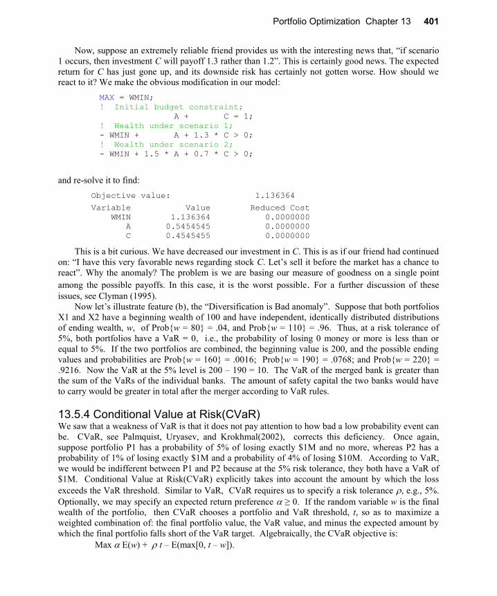
Portfolio Optimization Chapter 13 401
Now, suppose an extremely reliable friend provides us with the interesting news that, “if scenario
1 occurs, then investment C will payoff 1.3 rather than 1.2”. This is certainly good news. The expected
return for C has just gone up, and its downside risk has certainly not gotten worse. How should we
react to it? We make the obvious modification in our model:
MAX = WMIN;
! Initial budget constraint;
A + C = 1;
! Wealth under scenario 1;
- WMIN + A + 1.3 * C > 0;
! Wealth under scenario 2;
- WMIN + 1.5 * A + 0.7 * C > 0;
and re-solve it to find:
Objective value: 1.136364
Variable Value Reduced Cost
WMIN 1.136364 0.0000000
A 0.5454545 0.0000000
C 0.4545455 0.0000000
This is a bit curious. We have decreased our investment in C. This is as if our friend had continued
on: “I have this very favorable news regarding stock C. Let’s sell it before the market has a chance to
react”. Why the anomaly? The problem is we are basing our measure of goodness on a single point
among the possible payoffs. In this case, it is the worst possible. For a further discussion of these
issues, see Clyman (1995).
Now let’s illustrate feature (b), the “Diversification is Bad anomaly”. Suppose that both portfolios
X1 and X2 have a beginning wealth of 100 and have independent, identically distributed distributions
of ending wealth, w, of Prob{w = 80} = .04, and Prob{w = 110} = .96. Thus, at a risk tolerance of
5%, both portfolios have a VaR = 0, i.e., the probability of losing 0 money or more is less than or
equal to 5%. If the two portfolios are combined, the beginning value is 200, and the possible ending
values and probabilities are Prob{w = 160} = .0016; Prob{w = 190} = .0768; and Prob{w = 220} =
.9216. Now the VaR at the 5% level is 200 – 190 = 10. The VaR of the merged bank is greater than
the sum of the VaRs of the individual banks. The amount of safety capital the two banks would have
to carry would be greater in total after the merger according to VaR rules.
13.5.4 Conditional Value at Risk(CVaR) We saw that a weakness of VaR is that it does not pay attention to how bad a low probability event can
be. CVaR, see Palmquist, Uryasev, and Krokhmal(2002), corrects this deficiency. Once again,
suppose portfolio P1 has a probability of 5% of losing exactly $1M and no more, whereas P2 has a
probability of 1% of losing exactly $1M and a probability of 4% of losing $10M. According to VaR,
we would be indifferent between P1 and P2 because at the 5% risk tolerance, they both have a VaR of
$1M. Conditional Value at Risk(CVaR) explicitly takes into account the amount by which the loss
exceeds the VaR threshold. Similar to VaR, CVaR requires us to specify a risk tolerance , e.g., 5%.
Optionally, we may specify an expected return preference ≥ 0. If the random variable w is the final
wealth of the portfolio, then CVaR chooses a portfolio and VaR threshold, t, so as to maximize a
weighted combination of: the final portfolio value, the VaR value, and minus the expected amount by
which the final portfolio falls short of the VaR target. Algebraically, the CVaR objective is:
Max E(w) + t – E(max[0, t – w]).
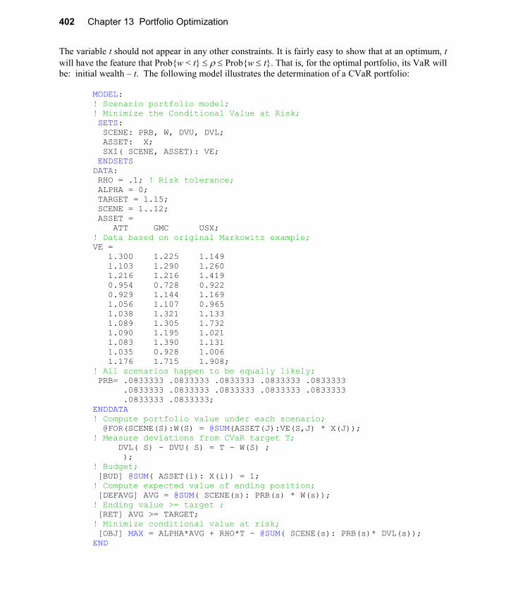
402 Chapter 13 Portfolio Optimization
The variable t should not appear in any other constraints. It is fairly easy to show that at an optimum, t
will have the feature that Prob{w < t} Prob{w t}. That is, for the optimal portfolio, its VaR will
be: initial wealth – t. The following model illustrates the determination of a CVaR portfolio:
MODEL:
! Scenario portfolio model;
! Minimize the Conditional Value at Risk;
SETS:
SCENE: PRB, W, DVU, DVL;
ASSET: X;
SXI( SCENE, ASSET): VE;
ENDSETS
DATA:
RHO = .1; ! Risk tolerance;
ALPHA = 0;
TARGET = 1.15;
SCENE = 1..12;
ASSET =
ATT GMC USX;
! Data based on original Markowitz example;
VE =
1.300 1.225 1.149
1.103 1.290 1.260
1.216 1.216 1.419
0.954 0.728 0.922
0.929 1.144 1.169
1.056 1.107 0.965
1.038 1.321 1.133
1.089 1.305 1.732
1.090 1.195 1.021
1.083 1.390 1.131
1.035 0.928 1.006
1.176 1.715 1.908;
! All scenarios happen to be equally likely;
PRB= .0833333 .0833333 .0833333 .0833333 .0833333
.0833333 .0833333 .0833333 .0833333 .0833333
.0833333 .0833333;
ENDDATA
! Compute portfolio value under each scenario;
@FOR(SCENE(S):W(S) = @SUM(ASSET(J):VE(S,J) * X(J));
! Measure deviations from CVaR target T;
DVL( S) - DVU( S) = T - W(S) ;
);
! Budget;
[BUD] @SUM( ASSET(i): X(i)) = 1;
! Compute expected value of ending position;
[DEFAVG] AVG = @SUM( SCENE(s): PRB(s) * W(s));
! Ending value >= target ;
[RET] AVG >= TARGET;
! Minimize conditional value at risk;
[OBJ] MAX = ALPHA*AVG + RHO*T - @SUM( SCENE(s): PRB(s)* DVL(s));
END

Portfolio Optimization Chapter 13 403
Part of the solution is:
Objective value: 0.09534855
Variable Value
RHO 0.1000000
ALPHA 0.000000
TARGET 1.150000
T 1.017901
AVG 1.150000
W( 1) 1.236780
W( 2) 1.168732
W( 3) 1.300991
W( 4) 0.940602
W( 5) 1.029482
W( 6) 1.017901
W( 7) 1.077774
W( 8) 1.358208
W( 9) 1.061111
W( 10) 1.103096
W( 11) 1.022858
W( 12) 1.482470
X( ATT) 0.581326
X( GMC) 0.000000
X( USX) 0.418674
The initial value of this portfolio was 1, so the VaR of this portfolio is 1 – T = -.017901. There are 12
scenarios. Notice that in only 1 of the 12, scenario 4, is the final wealth less than T = 1.017901. Thus,
in 1 outcome out of 12, or less than 10% of the outcomes, would the final value be less than 1.017901.
13.6 Scenario Model and Minimizing Downside Risk Minimizing the variance in return is appropriate if either:
1) the actual return is Normal-distributed or
2) the portfolio owner has a quadratic utility function.
In practice, it is difficult to show either condition holds. Thus, it may be of interest to use a more
intuitive measure of risk. One such measure is the downside risk, which intuitively is the expected
amount by which the return is less than a specified target return. The approach can be described if we
define:
T = user specified target threshold. When risk is disregarded, this is typically less than the
maximum expected return and greater than the return under the worst scenario.
Ys = amount by which the return under scenario s falls short of target.
= max{0, T Xi uis}

404 Chapter 13 Portfolio Optimization
The model in algebraic form is then:
Min Ps Ys ! Minimize expected downside risk
subject to
(compute deviation below target of each scenario, s):
Ys T + Xi uis 0
Xi = 1 (budget constraint)
Xi Ps uis r (desired return).
Notice this is just a linear program.
13.6.1 Semi-variance and Downside Risk The most common alternative suggested to variance as a measure of risk is some form of downside
risk. One such measure is semi-variance. It is essentially variance, except only deviations below the
mean are counted as risk. The scenario model is well suited to such measures. The previous scenario
model needs only a slight modification to convert it to a semi-variance model. The Y variables are
redefined to measure the deviation below the mean only, zero otherwise. The resulting model is:
MODEL:
! Scenario portfolio model;
! Minimize the semi-variance;
SETS:
SCENE/1..12/: PRB, R, DVU, DVL;
ASSET/ ATT, GMT, USX/: X;
SXI( SCENE, ASSET): VE;
ENDSETS
DATA:
TARGET = 1.15;
! Data based on original Markowitz example;
VE =
1.300 1.225 1.149
1.103 1.290 1.260
1.216 1.216 1.419
0.954 0.728 0.922
0.929 1.144 1.169
1.056 1.107 0.965
1.038 1.321 1.133
1.089 1.305 1.732
1.090 1.195 1.021
1.083 1.390 1.131
1.035 0.928 1.006
1.176 1.715 1.908;
! All scenarios happen to be equally likely;
PRB= .0833333 .0833333 .0833333 .0833333 .0833333
.0833333 .0833333 .0833333 .0833333 .0833333
.0833333 .0833333;
ENDDATA
! Compute value under each scenario;
@FOR(SCENE(S):R(S) = @SUM(ASSET(J):VE(S,J) * X(J));
! Measure deviations from average;
DVU( S) - DVL( S) = R(S) - AVG;);

Portfolio Optimization Chapter 13 405
! Budget;
[BUD] @SUM( ASSET: X) = 1;
! Compute expected value of ending position;
[DEFAVG] AVG = @SUM( SCENE: PRB * R);
! Target ending value;
[RET] AVG > TARGET;
! Minimize the semi-variance;
[OBJ] MIN = @SUM( SCENE: PRB * DVL^2);
END
The resulting solution is:
Optimal solution found at step: 4
Objective value: 0.8917110E-02
Variable Value Reduced Cost
R( 1) 1.238875 0.0000000
R( 2) 1.170760 0.0000000
R( 3) 1.294285 0.0000000
R( 4) 0.9329399 0.0000000
R( 5) 1.029848 0.0000000
R( 6) 1.022875 0.0000000
R( 7) 1.085554 0.0000000
R( 8) 1.345299 0.0000000
R( 9) 1.067442 0.0000000
R( 10) 1.113355 0.0000000
R( 11) 1.019688 0.0000000
R( 12) 1.479083 0.0000000
DVU( 1) 0.8887491E-01 0.0000000
DVU( 2) 0.2076016E-01 0.0000000
DVU( 3) 0.1442846 0.0000000
DVU( 4) 0.0000000 0.3617666E-01
DVU( 5) 0.0000000 0.2002525E-01
DVU( 6) 0.0000000 0.2118756E-01
DVU( 7) 0.0000000 0.1074092E-01
DVU( 8) 0.1952993 0.0000000
DVU( 9) 0.0000000 0.1375965E-01
DVU( 10) 0.0000000 0.6107114E-02
DVU( 11) 0.0000000 0.2171863E-01
DVU( 12) 0.3290833 0.0000000
DVL( 1) 0.0000000 0.8673617E-09
DVL( 2) 0.0000000 0.8673617E-09
DVL( 3) 0.0000000 0.8673617E-09
DVL( 4) 0.2170601 0.0000000
DVL( 5) 0.1201515 0.0000000
X( ATT) 0.5757791 0.0000000
X( GMT) 0.3858243E-01 0.0000000
X( USX) 0.3856385 0.0000000
Row Slack or Surplus Dual Price
BUD 0.0000000 0.1198420
DEFAVG 0.0000000 -0.9997334E-02
RET 0.0000000 -0.1197184
OBJ 0.8917110E-02 1.000000

406 Chapter 13 Portfolio Optimization
Notice the objective value is less than half that of the variance model. We would expect it to be at
most half, because it considers only the down (not the up) deviations. The most noticeable change in
the portfolio is substantial funds have been moved to USX from GMC. This is not surprising if you
look at the original data. In the years in which ATT performs poorly, USX tends to perform better than
GMC.
13.6.2 Downside Risk and MAD If the threshold for determining downside risk is the mean return, then minimizing the downside risk is
equivalent to minimizing the mean absolute deviation (MAD) about the mean. This follows easily
because the sum of deviations (not absolute) about the mean must be zero. Thus, the sum of deviations
above the mean equals the sum of deviations below the mean. Therefore, the sum of absolute
deviations is always twice the sum of the deviations below the mean. Thus, minimizing the downside
risk below the mean gives exactly the same recommendation as minimizing the sum of absolute
deviations below the mean. Konno and Yamazaki (1991) use the MAD measure to construct portfolios
from stocks on the Tokyo stock exchange.
13.6.3 Scenarios Based Directly Upon a Covariance Matrix If only a covariance matrix is available, rather than original data, then, not surprisingly, it is
nevertheless possible to construct scenarios that match the covariance matrix. The following example
uses just four scenarios to represent the possible returns from the three assets: ATT, GMC, and USX.
These scenarios have been constructed, using the methods of section 12.8.2, so they mimic behavior
consistent with the original covariance matrix:
MODEL:
SETS:
! Each asset has a variable value and an average return;
ASSET: X, RET;
! the variance of return at each scenario (which can be negative),
and the probability of it happening;
SCEN: Y, P;
! Return for each asset under each scenario;
COVMAT( SCEN, ASSET):ENTRY;
ENDSETS
DATA:
P = .25 .25 .25 .25; ! Four equi-likely scenarios;
ASSET = ATT GMC USX;
ENTRY = .9851237 1.304437 1.097669
1.193042 1.543131 1.756196
.9851237 .8842088 1.119948
1.193042 1.122902 .9645076;
RET = 1.089083 1.213667 1.234583;
ENDDATA
! Minimize the variance;
MIN = @SUM( SCEN(s): Y(s) * Y(s) * P(s));
! Compute the deviation from mean under each scenario;
@FOR(SCEN(s):Y(s) = @SUM(ASSET(J): ENTRY(s,J)* X(J)) - MEAN
);
! The Budget constraint;
@SUM(ASSET(j): X(j)) = 1;
! Define or compute the mean;

Portfolio Optimization Chapter 13 407
@SUM(ASSET(j): X * RET) = MEAN;
MEAN > 1.15;! Target return;
! The variance of each return can be negative;
@FOR(SCEN: @FREE(Y));
END
When solved, we get the familiar solution:
Optimal solution found at step: 4
Objective value: 0.2241380E-01
Variable Value Reduced Cost
MEAN 1.150000 0.0000000
X( ATT) 0.5300912 0.0000000
X( GMC) 0.3564126 0.0000000
X( USX) 0.1134962 0.0000000
RET( ATT) 1.089083 0.0000000
RET( GMC) 1.213667 0.0000000
RET( USX) 1.234583 0.0000000
Y( 1) -0.3829557E-01 0.0000000
Y( 2) 0.2317340 0.0000000
Y( 3) -0.1855416 0.0000000
Y( 4) -0.7894565E-02 0.0000000
P( 1) 0.2500000 0.0000000
P( 2) 0.2500000 0.0000000
P( 3) 0.2500000 0.0000000
P( 4) 0.2500000 0.0000000
ENTRY( 1, ATT) 0.9851237 0.0000000
ENTRY( 1, GMC) 1.304437 0.0000000
ENTRY( 1, USX) 1.097669 0.0000000
ENTRY( 2, ATT) 1.193042 0.0000000
ENTRY( 2, GMC) 1.543131 0.0000000
ENTRY( 2, USX) 1.756196 0.0000000
ENTRY( 3, ATT) 0.9851237 0.0000000
ENTRY( 3, GMC) 0.8842088 0.0000000
ENTRY( 3, USX) 1.119948 0.0000000
ENTRY( 4, ATT) 1.193042 0.0000000
ENTRY( 4, GMC) 1.122902 0.0000000
ENTRY( 4, USX) 0.9645076 0.0000000
Row Slack or Surplus Dual Price
1 0.2241380E-01 1.000000
2 0.0000000 0.1914778E-01
3 0.0000000 -0.1158670
4 0.0000000 0.9277079E-01
5 0.0000000 0.3947280E-02
6 0.0000000 0.3621391
7 0.0000000 -0.3538852
8 0.0000000 -0.3538841
Notice the objective function value and the allocation of funds over ATT, GMC, and USX are
essentially identical to our original portfolio example.

408 Chapter 13 Portfolio Optimization
13.7 Hedging, Matching and Program Trading
13.7.1 Portfolio Hedging Given a “benchmark” portfolio B, we say we hedge B if we construct another portfolio C such that,
taken together, B and C have essentially the same return as B, but lower risk than B. Typically, our
portfolio B contains certain components that cannot be removed. Thus, we want to buy some
components negatively correlated with the existing ones. Examples are:
a) An airline knows it will have to purchase a lot of fuel in the next three months. It would like
to be insulated from unexpected fuel price increases.
b) A farmer is confident his fields will yield $200,000 worth of corn in the next two months. He
is happy with the current price for corn. Thus, would like to “lock in” the current price.
13.7.2 Portfolio Matching, Tracking, and Program Trading Given a benchmark portfolio B, we say we construct a matching or tracking portfolio if we construct a
new portfolio C that has stochastic behavior very similar to B, but excludes certain instruments in B.
Example situations are:
a) A portfolio manager does not wish to look bad relative to some well-known index of
performance such as the S&P 500, but for various reasons cannot purchase certain
instruments in the index.
b) An arbitrageur with the ability to make fast, low-cost trades wants to exploit market
inefficiencies (i.e., instruments mispriced by the market). If he can construct a portfolio that
perfectly matches the future behavior of the well-defined portfolio, but costs less today, then
he has an arbitrage profit opportunity (if he can act before this “mispricing” disappears).
c) A retired person is concerned mainly about inflation risk. In this case, a portfolio that tracks
inflation is desired.
As an example of (a), a certain so-called “green” mutual fund will not include in its portfolio
companies that derive more than 2% of their gross revenues from the sale of military weapons, own
directly or operate nuclear power plants, or participate in business related to the nuclear fuel cycle.
The following table, for example, compares the performance of six Vanguard portfolios with the
indices the portfolios were designed to track; see Vanguard (1995):
Total Return Six Months Ended June 30, 1995
Vanguard Portfolio Comparative Index Portfolio Name Growth Growth Index Name
500 Portfolio +20.1% +20.2% S&P500
Growth Portfolio +21.1 +21.2 S&P500/BARRA Growth
Value Portfolio +19.1 +19.2 S&P500/BARRA Value
Extended Market Portfolio +17.1% +16.8% Wilshire 4500 Index
SmallCap Portfolio +14.5 +14.4 Russell 2000 Index
Total Stock Market
Portfolio
+19.2% +19.2% Wilshire 5000 Index
Notice, even though there is substantial difference in the performance of the portfolios, each
matches its benchmark index quite well.

Portfolio Optimization Chapter 13 409
13.8 Methods for Constructing Benchmark Portfolios A variety of approaches has been used for constructing hedging and matching portfolios. For matching
portfolios, an intuitive approach has been to generalize the Markowitz model, so the objective is to
minimize the variance in the difference in return between the target portfolio and the tracking portfolio.
A useful way to think about hedging or matching of a benchmark is to think of it as our being
forced to include the benchmark or its negative in our portfolio. Suppose the benchmark is a simple
index such as the S&P500. If our measure of risk is variance, then proceed as follows:
1. Include the benchmark in the covariance matrix just like any other instrument, except do
not include it in the budget constraint. We presume we have a budget of $1 to invest in
the controllable, non-benchmark portion of our portfolio.
2. To get a “matching” portfolio (e.g., one that mimics the S&P 500), set the value of the
benchmark factor to 1. The essential effect is the off diagonal covariance terms are
negated in the row/column of the benchmark factor. Effectively, we have shorted the
factor. If we can get the total variance to zero, we have perfectly matched the randomness
of the benchmark.
3. To get a “hedging” portfolio (e.g., one as negatively correlated with the S&P 500 as
possible), set the value of the benchmark factor to +1. Thus, we will compose the rest of
the portfolio to counteract the effect of the factor we are stuck with having in the
portfolio.
One might even want to drop the budget constraint. The solution will then tell you how much to
invest in the controllable portfolio to get the best possible hedge or match per $ of the benchmark.

410 Chapter 13 Portfolio Optimization
The following model illustrates the extension of the Markowitz approach to the hedging case
where we want to “cancel out” some benchmark. In the case of GMC, it could be that our decision
maker works for GMC and thus has his fortunes unavoidably tied to those of GMC. He might wish to
find a portfolio negatively correlated with GMC:
MODEL:
!Generic Markowitz portfolio Hedging model(PORTHEDG);
! We want to hedge the first or "benchmark" asset
with the remaining ones;
SETS:
ASSET/ GMC ATT USX/: RET, X;
TMAT( ASSET, ASSET) | &1 #GE# &2: COV;
ENDSETS
DATA:
! The expected returns;
RET = 1.21367, 1.089083, 1.23458;
! Covariance matrix;
COV =
.05839170
.01240721 .01080754
.05542639 .01307513 .09422681;
! The desired return;
TARGET = 1.15;
ENDDATA
!-------------------------------------------------;
! Min the var in portfolio return;
[OBJ] MIN= ( @SUM( ASSET( I):
COV( I, I) * X( I)^2) +
2 * @SUM( TMAT( I, J) | I #NE# J:
COV( I, J) * X( I) * X( J))) ;
!We are stuck with the first asset in the portfolio;
X( 1) = 1;
! Budget constraint(applies to remaining assets);
[BUDGET] @SUM( ASSET( I)| I #GT# 1: X( I)) = 1;
! Return requirement(applies to remaining assets);
[RETURN] @SUM( ASSET( I)| I #GT# 1:
RET( I) * X( I)) >= TARGET;
END
The solution is:
Optimal solution found at step: 4
Objective value: 0.1457632
Variable Value Reduced Cost
X( GMC) 1.000000 0.0000000
X( ATT) 0.5813178 0.0000000
X( USX) 0.4186822 0.0000000
Thus, our investor puts more of the portfolio in ATT than in USX (whose fortunes are more closely
tied to those of GMC).

Portfolio Optimization Chapter 13 411
The following model illustrates the extension of the Markowitz approach to the matching case
where we want to construct a portfolio that mimics or matches a benchmark portfolio. In this case, we
want to match the S&P500, but limit ourselves to investing in only ATT, GMC, and USX:
MODEL:
!Gen. Markowitz portfolio Matching model(PORTMTCH);
! We want to match the first or "benchmark" asset
with the remaining ones;
SETS:
ASSET/ SP500 ATT GMC USX/: RET, X;
TMAT( ASSET, ASSET) | &1 #GE# &2: COV;
ENDSETS
DATA:
! The expected returns;
RET = 1.191458 1.089083, 1.21367, 1.23458;
! Covariance matrix;
COV =
.02873661
.01266498 .01080754
.03562763 .01240721 .05839170
.04378880 .01307513 .05542639 .09422681;
! The desired return;
TARGET = 1.191458;
ENDDATA
!-------------------------------------------------;
! Min the var in portfolio return;
[OBJ] MIN = (@SUM( ASSET(I): COV(I, I) * X( I)^2)
+ 2 * @SUM( TMAT( I, J) | I #NE# J:
COV( I, J) * X( I) * X( J))) ;
!Matching is equivalent to being short the benchmark;
X( 1) = -1;
@FREE( X( 1));
! Budget constraint(applies to remaining assets);
[BUDGET] @SUM( ASSET( I)| I #GT# 1: X( I)) = 1;
! Return requirement(applies to remaining assets);
[RETURN] @SUM( ASSET( I)| I #GT# 1:
RET( I) * X( I)) >= TARGET;
END
The solution is:
Optimal solution found at step: 4
Objective value: 0.5245968E-02
Variable Value Reduced Cost
X( SP500) -1.000000 0.0000000
X( ATT) 0.2276635 0.0000000
X( GMC) 0.4781277 0.0000000
X( USX) 0.2942089 -0.1266506E-07

412 Chapter 13 Portfolio Optimization
13.8.1 Scenario Approach to Benchmark Portfolios
If we use the scenario approach, then the hedging model looks as follows:
MODEL: ! (PRTSHDGE);
! Scenario portfolio model, Hedge 1st asset;
! Minimize the variance;
SETS:
SCENE/1..12/: PRB, R, DVU, DVL;
ASSET/ GMT, ATT, USX/: X;
SXA( SCENE, ASSET): VE;
ENDSETS
DATA:
! Data based on original Markowitz example;
VE =
1.225 1.300 1.149
1.290 1.103 1.260
1.216 1.216 1.419
0.728 0.954 0.922
1.144 0.929 1.169
1.107 1.056 0.965
1.321 1.038 1.133
1.305 1.089 1.732
1.195 1.090 1.021
1.390 1.083 1.131
0.928 1.035 1.006
1.715 1.176 1.908;
! All scenarios happen to be equally likely;
PRB= .0833333 .0833333 .0833333 .0833333 .0833333
.0833333 .0833333 .0833333 .0833333 .0833333
.0833333 .0833333;
! The desired return;
TARGET = 1.15;
ENDDATA
! Minimize risk;
[OBJ] MIN = @SUM( SCENE: PRB * ( DVL + DVU) ^ 2);
!We are stuck with having asset 1 in the portfolio;
X( 1) = 1;
!Compute hedging portfolio value under each scenario;
@FOR( SCENE( S):
R( S)=
@SUM( ASSET( J)| J #GT# 1: VE( S, J) * X( J));
! Measure deviations hedge + benchmark from target;
DVU( S) - DVL( S) =
( R(S) + VE( S, 1))/ 2 - TARGET;
);
! Budget constraint(applies to remaining assets);
[BUDGET] @SUM( ASSET( J)| J #GT# 1: X( J)) = 1;
! Compute expected value of ending position;
[DEFAVG] AVG = @SUM( SCENE: PRB * R);
! Target ending value;
[RET] AVG > TARGET;
END

Portfolio Optimization Chapter 13 413
With a solution:
Optimal solution found at step: 4
Objective value: 0.3441714E-01
Variable Value Reduced Cost
X( GMT) 1.000000 0.0000000
X( ATT) 0.5813256 0.0000000
X( USX) 0.4186744 0.0000000
Notice we get the same portfolio as with the Markowitz model.
A scenario model for constructing a portfolio matching the S&P500 looks as follows:
MODEL: ! Scenario model, Match 1st asset(PRTSMTCH);
! Minimize the variance;
SETS:
SCENE/1..12/: PRB, R, DVU, DVL;
ASSET/ SP500 ATT GMT USX/: X;
SXA( SCENE, ASSET): VE;
ENDSETS
DATA:
! Data based on original Markowitz example;
VE =
! S&P500 ATT GMC USX;
1.258997 1.3 1.225 1.149
1.197526 1.103 1.29 1.26
1.364361 1.216 1.216 1.419
0.919287 0.954 0.728 0.922
1.05708 0.929 1.144 1.169
1.055012 1.056 1.107 0.965
1.187925 1.038 1.321 1.133
1.31713 1.089 1.305 1.732
1.240164 1.09 1.195 1.021
1.183675 1.083 1.39 1.131
0.990108 1.035 0.928 1.006
1.526236 1.176 1.715 1.908;
! All scenarios happen to be equally likely;
PRB= .0833333 .0833333 .0833333 .0833333 .0833333
.0833333 .0833333 .0833333 .0833333 .0833333
.0833333 .0833333;
! The desired return;
TARGET = 1.191458;
ENDDATA
! Minimize risk;
[OBJ] MIN = @SUM( SCENE: PRB * ( DVL + DVU) ^ 2);
! Compute portfolio value under each scenario;
@FOR( SCENE( S):
R( S) =
@SUM( ASSET( J)| J #GT# 1: VE( S, J) * X( J));
! Measure deviations of portfolio from benchmark;
DVU( S) - DVL( S) = ( R(S) - VE( S, 1));
);
! Budget constraint(applies to remaining assets);
[BUDGET] @SUM( ASSET( J)| J #GT# 1: X( J)) = 1;

414 Chapter 13 Portfolio Optimization
! Compute expected value of ending position;
[DEFAVG] AVG = @SUM( SCENE: PRB * R);
! Target ending value;
[RET] AVG > TARGET;
END
The solution is:
Optimal solution found at step: 7
Objective value: 0.4808974E-02
Variable Value Reduced Cost
X( SP500) 0.0000000 0.0000000
X( ATT) 0.2276583 0.0000000
X( GMT) 0.4781151 0.0000000
X( USX) 0.2942266 0.0000000
Notice we get the same portfolio as with the Markowitz model.
The two scenario models both used variance for the measure of risk relative to the benchmark. It is
easy to modify them, so more asymmetric risk measures, such as downside risk, could be used.
13.8.2 Efficient Benchmark Portfolios We say a portfolio is on the efficient frontier if there is no other portfolio that has both higher expected
return and lower risk.
Let:
ri = expected return on asset i,
t = an arbitrary target return for the portfolio.
A portfolio, with weight mi on asset i, is efficient if there exists some target t for which the
portfolio is a solution to the problem:
Minimize risk
subject to
i
n
0
mi = 1 (budget constraint)
i
m
0ri mi t (return target constraint).
Portfolio managers are frequently evaluated on their performance relative to some benchmark
portfolio. Let bi = the weight on asset i in the benchmark portfolio. If the benchmark portfolio is not on
the efficient frontier, then an interesting question is: What are the weights of the portfolio on the
efficient frontier that is closest to the benchmark portfolio in the sense that the risk of the efficient
portfolio relative to the benchmark is minimized?

Portfolio Optimization Chapter 13 415
There is a particularly simple answer when the measure of risk is portfolio variance, there is a
risk-free asset, borrowing is allowed at the risk-free rate, and short sales are permitted. Let m0 = the
weight on the risk-free asset. An elegant result, in this case, is that there is a so-called “market”
portfolio with weights mi on asset i, such that effectively only m0 varies as the return target varies.
Specifically, there are constants mi, for i = 1, 2, . . . , n, such that the weight on asset i is simply (1 m0)
mi. Define:
q = 1 m0 = weight to put on the market portfolio,
Ri = random return on asset i.
Then the variance of any efficient portfolio relative to the benchmark portfolio can be written as:
var( i
n
1Ri[qmi bi])
= i
n
1
(qmi bi)2 var (Ri) + 2
j
i
(qmi bi)(qm j bj) Cov(Ri,R j).
Setting the derivative of this expression with respect to q equal to zero gives the result:
q = i
n
1
mi bi var (Ri) + j
i (mi bj mj bi) Cov (Ri, R j)
____________________________________________________________________________________________________________________________
i
n
1
mi2 var (Ri) + 2
j
imi mj Cov (Ri, Rj)
For example, if the benchmark portfolio is on the efficient frontier with weight b0 on the risk-free
asset, then bi = (1 b0)mi and therefore q = 1 b0.
Thus, a manager who is told to outperform the benchmark portfolio {b0, b1, . . ., bn} should
perhaps, in fact, be compensated according to his performance relative to the efficient portfolio given
by q above.
13.8.3 Efficient Formulation of Portfolio Problems The amount of time it takes to solve a mathematical model may depend dramatically on how the model
is formulated. This phenomenon is well known in integer programming circles. Below, we illustrate
the same phenomenon for nonlinear programs. We give several different, but mathematically
equivalent, formulations of a portfolio optimization model.
Formulation 1
Minimize j
n
i
n
11
qij xi xj
subject to
j
n
1xj = 1
j
n
1rj xj = r0

416 Chapter 13 Portfolio Optimization
Formulation 2
We can exploit the fact that the covariance matrix is symmetric to rewrite the objective as:
Min i
n
1
xi (qii xi + 2 j=i+1
n
qij xj )
subject to
j
n
1
xj = 1
j
n
1
rj xj = r0
Formulation 3
We can separately compute the term multiplying xi in the objective to get the formulation:
Minimize i
n
1xi wi
subject to
For each i;
wi = qii xi + 2 j=i+1
n
qij xj, wi a free variable
j
n
1xj = 1
j
n
1rj xj = r0
We solved a specific instance of these formulations for a data set based on the performance of 19
stocks on the New York Stock exchange (IBM, Xerox, ATT, etc.). These models were solved as
general nonlinear programs. The fact they were quadratic programs was not exploited.
The solution time in seconds for each formulation was:
Formulation Time in seconds
1 2.16
2 1.5
3 0.82
Why the dramatic differences in solution time?
The advantage of formulation (2) over (1) is relatively obvious. Each function evaluation of the
objective in (1) requires approximately 2 n n multiplications (2 multiplications for each of
approximately n n terms). For (2), the equivalent figure is about n + n n/2 multiplications.
Formulation (3) has essentially the same number of multiplications as (2). However, about n n/2
of them appear in linear constraints. The number of constraints has dramatically increased. However,
these constraints are linear and the technology for efficiently processing linear constraints is well
developed.

Portfolio Optimization Chapter 13 417
13.9 Cholesky Factorization for Quadratic Programs There is another formulation comparable to formulation (3), but even more compact. Given a
covariance matrix {qij}, one can compute its “square root,” the so-called Cholesky factorization, to
give a lower triangular matrix {Lij}. The new formulation is then:
Minimize j
n
1wj
2
subject to
For each j:
wj = i=j+1
n
Lij xj, wj a free variable
j
n
1xj = 1
j
n
1rj xj = r0
Notice it is approximately identical in structure to formulation (3) except it has only n rather than
2n variables in the objective.
For the reader comfortable with matrix notation, the transformation is easy to explain. Given the
covariance matrix Q and a lower triangular matrix L such that:
L L' = Q, where L' denotes transpose,
our objective is to:
Minimize x Q x' = x L L' x'
If we set w = x L, then our objective is simply:
Minimize w w'
subject to
w = x L.
A LINGO model using Cholesky decomposition and applied to our three-asset example is shown
below:
MODEL:! Cholesky factorization Portfolio model;
SETS:
ASSET: AMT, RET, CW;
COVMAT( ASSET, ASSET): VARIANCE;
MAT(ASSET,ASSET)| &1 #GE# &2: L; !Cholesky factor;
ENDSETS
DATA:
ASSET = ATT GMC USX;
!Covariance matrix and expected returns;
VARIANCE = .01080754 .01240721 .01307513
.01240721 .05839170 .05542639
.01307513 .05542639 .09422681;
RET = .0890833 .213667 .234583;
ENDDATA
! Minimize variance;
[VAR] MIN = @SUM( ASSET( I): CW( I) * CW( I));

418 Chapter 13 Portfolio Optimization
! Use exactly 100% of the starting budget;
[BUDGET] @SUM( ASSET: AMT) = 1;
! Required wealth at end of period;
[RETURN] @SUM( ASSET: AMT * RET) > .15;
! Compute contributions to variance, CW();
@FOR( ASSET( J):
@FREE( CW( J));
CW( J) = @SUM( MAT( I, J): L( I, J) * AMT( I));
);
!Compute the Cholesky factor L, so LL'= VARIANCE;
@FOR( ASSET( I):
@FOR( MAT( I, J)| J #LT# I:
L(I,J) = ( VARIANCE( I, J) - @SUM( MAT( I, K)|
K #LT# J: L( I, K) * L( J, K)))/ L( J, J);
);
L(I,I) = ( VARIANCE( I, I) - @SUM( MAT( I, K)|
K #LT# I: L( I, K) * L( I, K)))^.5;
);
END
Part of the solution report is shown below:
Optimal solution found at step: 4
Objective value: 0.2241375E-01
Variable Value Reduced Cost
AMT( ATT) 0.5300926 0.0000000
AMT( GMC) 0.3564106 0.0000000
AMT( USX) 0.1134968 0.4492217E-08
RET( ATT) 0.8908330E-01 0.0000000
RET( GMC) 0.2136670 0.0000000
RET( USX) 0.2345830 0.0000000
CW( ATT) 0.1119192 0.0000000
CW( GMC) 0.9671834E-01 0.0000000
CW( USX) 0.2309568E-01 0.0000000
VARIANCE( ATT, ATT) 0.1080754E-01 0.0000000
VARIANCE( ATT, GMC) 0.1240721E-01 0.0000000
VARIANCE( ATT, USX) 0.1307513E-01 0.0000000
VARIANCE( GMC, ATT) 0.1240721E-01 0.0000000
VARIANCE( GMC, GMC) 0.5839170E-01 0.0000000
VARIANCE( GMC, USX) 0.5542639E-01 0.0000000
VARIANCE( USX, ATT) 0.1307513E-01 0.0000000
VARIANCE( USX, GMC) 0.5542639E-01 0.0000000
VARIANCE( USX, USX) 0.9422681E-01 0.0000000
L( ATT, ATT) 0.1039593 0.0000000
L( GMC, ATT) 0.1193468 0.0000000
L( GMC, GMC) 0.2101144 0.0000000
L( USX, ATT) 0.1257716 0.0000000
L( USX, GMC) 0.1923522 0.0000000
L( USX, USX) 0.2034919 0.0000000
Row Slack or Surplus Dual Price
VAR 0.2241375E-01 -1.000000
BUDGET 0.0000000 0.8255034E-02
RETURN 0.0000000 -0.3538836

Portfolio Optimization Chapter 13 419
13.10 Positive Definiteness Constraints An important feature of a valid covariance matrix is that it must be positive semi-definite.
Loosely speaking, this means the diagonal of the matrix must be large relative to the off-diagonal
elements. More precisely, if Q is a square matrix, e.g., a covariance matrix, then for any vector x, we
must have, in matrix notation, x’Qx ≥ 0. In terms of portfolio optimization, if the x vector represents
the amount invested in a set of assets, and Q is the covariance matrix, then x’Qx is the variance of the
portfolio and we expect, and in fact require, that this variane be ≥ 0. Now suppose that the Q matrix is
not given in advance, but rather the the elements of Q are decision variables, and we are constraining
these elements of the matrix so that Q is positive semi-definite. A mathematical program in which we
allow such constraints is called a Semi-Definite Program, or SDP for short. LINGO has a simple
constraint type to indicate that a matrix Q must be positive semi-definite, namely, @POSD( Q);.
To illustrate the usefulness of this capability, suppose that we asked three experts to estimate
the three covariances between three stocks and we obtained the following “guesstimate” of the
correlation matrix: 1.000000 0.6938961 -0.1097276
0.6938961 1.000000 0.7972293
-0.1097276 0.7972293 1.000000 ;
Although not immediately obvious, it happens to be the case that this matrix is not quite positive-semi-
definte, so it is not a valid correlation matrix. So a reasonable thing to try to do is to make minimal
adjustments to the off-diagonal elements to convert this matrix to a positive semi-definite matrix. The
following LINGO model witll do this. Notice the following: 1) Because the matrix is symmetric,
LINGO only requires that you enter the lower triangle of the matrix. 2) The last statement in the model
is @POSD( QFIT), i.e., we want the fitted matrix to be positive semi-definite, and 3) Our objective is
to minimize the sum of the squared differences between the original guessed matrix and the fitted
matrix.
SETS:
VEC;
MAT( VEC,VEC) | &1 #GE# &2: QINI, QADJ, QFIT;
ENDSETS
DATA:
VEC = 1..3;
! Our initial estimate of the correlation matrix,
( May not be positive semi-definite);
QINI =
1.000000
0.6938961 1.000000
-0.1097276 0.7972293 1.000000 ;
ENDDATA
! Minimize the amount of adjustments we have
to make to the off-diagonal terms of
our initial estimated matrix...;
MIN = @SUM( MAT(i,j) | i #GT# j: QADJ(i,j)^2);
! Fitted matrix = initial + adjustment;
@FOR( MAT(i,j) | i #GT# j:
QFIT(i,j) = QINI(i,j) + QADJ(i,j);
! Off diagonal adjustments or fitted
might be < 0;

420 Chapter 13 Portfolio Optimization
@FREE( QADJ(i,j));
@FREE( QFIT(i,j));
);
! Diagonal terms stay at 1;
@FOR( VEC(i):
QFIT(i,i) = QINI(i,i);
QADJ(i,i) = 0;
);
! The adusted/fitted matrix must be
Positive semi-definite;
@POSD( QFIT);
When solved, we get the fitted matrix:
1.000000
0.6348391 1.000000
-0.0640226 0.7304152 1.000000
Notice that in the fitted matrix, the off-diagonal elements have been moved closer to 0. There are a
number of other applications of the @POSD( ) or SDP capability. Look at the MODELS library at
www.lindo.com under the keyword of @POSD.
13.11 Problems 1. You are considering three stocks, IBM, GM, and Georgia-Pacific (GP), for your stock portfolio.
The covariance matrix of the yearly percentage returns on these stocks is estimated to be:
IBM GM GP
IBM 10 2.5 1
GM 2.5 4 1.5
GP 1 1.5 9
Thus, if equal amounts were invested in each, the variance would be proportional to 10 + 4 +
9 + 2 (2.5 + 1 + 1.5). The predicted yearly percentage returns for IBM, GM, and GP are 9, 6 and 5,
respectively. Find a minimum variance portfolio of these three stocks for which the yearly return
is at least 7, at most 80% of the portfolio is invested in IBM, and at least 10% is invested in GP.
2. Modify your formulation of problem 1 to incorporate the fact that your current portfolio is 50%
IBM and 50% GP. Further, transaction costs on a buy/sell transaction are 1% of the amount traded.

Portfolio Optimization Chapter 13 421
3. The manager of an investment fund hypothesizes that three different scenarios might characterize
the economy one year hence. These scenarios are denoted Green, Yellow and Red and subjective
probabilities 0.7, 0.1, and 0.2 are associated with them. The manager wishes to decide how a
model portfolio should be allocated among stocks, bonds, real estate and gold in the face of these
possible scenarios. His estimated returns in percent per year as a function of asset and scenario are
given in the table below:
Stocks Bonds Real Estate Gold
Green 9 7 8 -2
Yellow 1 5 10 12
Red 10 4 -1 15
Formulate and solve the asset allocation problem of minimizing the variance in return subject
to having an expected return of at least 6.5.
4. Consider the ATT/GMC/USX portfolio problem discussed earlier. The desired or target rate of
return in the solved model was 15%.
a) Suppose we desire a 16% rate of return. Using just the solution report, what can you
predict about the standard deviation in portfolio return of the new portfolio?
b) We illustrated the situation where the opportunity to invest money risk-free at 5% per
year becomes available. That is, this fourth option has zero variance and zero covariance.
Now, suppose the risk-free rate is 4% per year rather than 5%. As before, there is no limit
on how much can be invested at 4%. Based on only the solution report available for the
original version of the problem (where the desired rate of return is 15% per year), discuss
whether this new option is attractive when the desired return for the portfolio is 15%.
c) You have $100,000 to invest. What modifications would need to be made to the original
ATT/GMC/USX model, so the answers in the solution report would come in the
appropriate units (e.g., no multiplying of the numbers in the solution by 100,000)?
d) What is the estimated standard deviation in the value of your end-of-period portfolio in
(c) if invested as the solution recommends?
Recommended