arX

iv:0

907.

4698

v1 [

stat

.ME

] 27

Jul

200

91

Shrinkage Algorithms for MMSE Covariance

EstimationYilun Chen, Ami Wiesel, Yonina C. Eldar and Alfred O. Hero III

Abstract

We address covariance estimation in the sense of minimum mean-squared error (MMSE) for Gaussian

samples. Specifically, we consider shrinkage methods whichare suitable for high dimensional problems

with a small number of samples (largep smalln). First, we improve on the Ledoit-Wolf (LW) method by

conditioning on a sufficient statistic. By the Rao-Blackwell theorem, this yields a new estimator called

RBLW, whose mean-squared error dominates that of LW for Gaussian variables. Second, to further reduce

the estimation error, we propose an iterative approach which approximates the clairvoyant shrinkage

estimator. Convergence of this iterative method is established and a closed form expression for the limit

is determined, which is referred to as the oracle approximating shrinkage (OAS) estimator. Both RBLW

and OAS estimators have simple expressions and are easily implemented. Although the two methods are

developed from different persepctives, their structure isidentical up to specified constants. The RBLW

estimator provably dominates the LW method. Numerical simulations demonstrate that the OAS approach

can perform even better than RBLW, especially whenn is much less thanp. We also demonstrate the

performance of these techniques in the context of adaptive beamforming.

Index Terms

Covariance estimation, shrinkage, minimum mean-squared error (MMSE), beamforming

Y. Chen, A. Wiesel and A. O. Hero are with the Department of Electrical Engineering and Computer Science, University of

Michigan, Ann Arbor, MI 48109, USA. Tel: (734) 763-0564, Fax: (734) 763-8041. Emails:{yilun,amiw,hero}@umich.edu.

Y. C. Eldar is with the Technion - Israel Institute of Technology, Haifa, Israel 32000. Email: yonina@ee.technion.ac.il.

This research was partially supported by the AFOSR grant FA9550-06-1-0324 and NSF grant CCF 0830490. The work of

A. Wiesel was supported by a Marie Curie Outgoing International Fellowship within the 7th European Community Framework

Programme.

July 27, 2009 DRAFT

2

I. INTRODUCTION

Covariance matrix estimation is a fundamental problem in signal processing and related fields. Many

applications varying from array processing [12] to functional genomics [17] rely on accurately estimated

covariance matrices. In recent years, estimation of high dimensionalp×p covariance matrices under small

sample sizen has attracted considerable interest. Examples include classification on gene expression from

microarray data, financial forecasting, spectroscopic imaging, brain activation mapping from fMRI and

many others. Standard estimation methods perform poorly inthese largep small n settings. This is the

main motivation for this work.

The sample covariance is a common estimate for the unknown covariance matrix. When it is invertible,

the sample covariance coincides with the classical maximumlikelihood estimate. However, while it is

an unbiased estimator, it does not minimize the mean-squared error (MSE). Indeed, Stein demonstrated

that superior performance may be obtained by shrinking the sample covariance [2], [3]. Since then,

many shrinkage estimators have been proposed under different performance measures. For example, Haff

[4] introduced an estimator inspired by the empirical Bayesapproach. Dey and Srinivasan [5] derived

a minimax estimator under Stein’s entropy loss function. Yang and Berger [6] obtained expressions for

Bayesian estimators under a class of priors for the covariance. These works addressed the case of invertible

sample covariance whenn ≥ p. Recently, Ledoit and Wolf (LW) proposed a shrinkage estimator for the

casen < p which asymptotically minimizes the MSE [8]. The LW estimator is well conditioned for small

sample sizes and can thus be applied to high dimensional problems. In contrast to previous approaches,

they show that performance advantages are distribution-free and not restricted to Gaussian assumptions.

In this paper, we show that the LW estimator can be significantly improved when the samples are in fact

Gaussian. Specifically, we develop two new estimation techniques that result from different considerations.

The first follows from the Rao-Blackwell theorem, while the second is an application of the ideas of [11]

to covariance estimation.

We begin by providing a closed form expression for the optimal clairvoyant shrinkage estimator under

an MSE loss criteria. This estimator is an explicit functionof the unknown covariance matrix that can

be used as an oracle performance bound. Our first estimator isobtained by applying the well-known

Rao-Blackwell theorem [31] to the LW method, and is therefore denoted by RBLW. Using several

nontrivial Haar integral computations, we obtain a simple closed form solution which provably dominates

the LW method in terms of MSE. We then introduce an iterative shrinkage estimator which tries to

approximate the oracle. This approach follows the methodology developed in [11] for the case of linear

July 27, 2009 DRAFT

3

regression. Beginning with an initial naive choice, each iteration is defined as the oracle solution when

the unknown covariance is replaced by its estimate obtainedin the previous iteration. Remarkably, a

closed form expression can be determined for the limit of these iterations. We refer to the limit as the

oracle approximating shrinkage (OAS) estimator.

The OAS and RBLW solutions have similar structure that is related to a sphericity test as discussed in

[18]–[20]. Both OAS and RBLW estimators are intuitive, easyto compute and perform well with finite

sample size. The RBLW technique provably dominates LW. Numerical results demonstrate that for small

sample sizes, the OAS estimator is superior to both the RBLW and the LW methods.

To illustrate the proposed covariance estimators we apply them to problems of time series analysis

and array signal processing. Specifically, in the context oftime series analysis we establish performance

advantages of OAS and RBLW to LW for covariance estimation inautoregressive models and in fractional

Brownian motion models, respectively. In the context of beamforming, we show that RBLW and OAS

can be used to significantly improve the Capon beamformer. In[12] a multitude of covariance matrix

estimators were implemented in Capon beamformers, and the authors reported that the LW approach

substantially improves performance as compared to other methods. We show here that even better

performance can be achieved by using the techniques introduced in this paper.

The paper is organized as follows. Section 2 formulates the problem. Section 3 introduces the oracle

estimator together with the RBLW and OAS methods. Section 4 represents numerical simulation results

and applications in adaptive beamforming. Section 5 summarizes our principal conclusions. The proofs

of theorems and lemmas are provided in the Appendix.

Notation: In the following, we depict vectors in lowercase boldface letters and matrices in uppercase

boldface letters.(·)T and (·)H denote the transpose and the conjugate transpose, respectively. Tr (·),

‖·‖F , and det(·) are the trace, the Frobenius norm, and the determinant of a matrix, respectively. Finally,

A ≺ B means that the matrixB − A is positive definite, andA ≻ B means that the matrixA − B is

positive definite.

II. PROBLEM FORMULATION

Let {xi}ni=1 be a sample of independent identical distributed (i.i.d.)p-dimensional Gaussian vectors

with zero mean and covarianceΣ. We do not assumen ≥ p. Our goal is to find an estimatorΣ ({xi}ni=1)

which minimizes the MSE:

E

{∥∥∥Σ ({xi}ni=1) − Σ

∥∥∥2

F

}. (1)

July 27, 2009 DRAFT

4

It is difficult to compute the MSE ofΣ ({xi}ni=1) without additional constraints and therefore we

restrict ourselves to a specific class of estimators that employ shrinkage [1], [7]. The unstructured classical

estimator ofΣ is the sample covarianceS defined as

S =1

n

n∑

i=1

xixTi . (2)

This estimator is unbiasedE{S} = Σ, and is also the maximum likelihood solution ifn ≥ p. However,

it does not necessarily achieve low MSE due to its high variance and is usually ill-posed for largep

problems. On the other hand, we may consider a naive but most well-conditioned estimate forΣ:

F =Tr(S)

pI. (3)

This “structured” estimate will result in reduced variancewith the expense of increasing the bias. A

reasonable tradeoff between low bias and low variance is achieved by shrinkage ofS towardsF, resulting

in the following class of estimators:

Σ = (1 − ρ)S + ρF. (4)

The estimatorΣ is characterized by the shrinkage coefficientρ, which is a parameter between 0 and 1

and can be a function of the observations{xi}ni=1. The matrixF is referred to as the shrinkage target.1

Throughout the paper, we restrict our attention to shrinkage estimates of the form (4). Our goal is

to find a shrinkage coefficientρ that minimizes the MSE (1). As we show in the next section, the

optimal ρ minimizing the MSE depends in general on the unknownΣ and therefore in general cannot

be implemented. Instead, we propose two different approaches to approximate the optimal shrinkage

coefficient.

III. SHRINKAGE ALGORITHMS

A. The Oracle estimator

We begin by deriving a clairvoyant oracle estimator that uses an optimal nonrandom coefficient to

minimize the mean-squared error. In the following subsections we will show how to approximate the

oracle using implementable data-driven methods.

1The convex combination in (4) can be generalized to the linear combination ofbS and bF. The reader is referred to [13] for

further discussion.

July 27, 2009 DRAFT

5

The oracle estimateΣO is the solution to

minρ

E

{∥∥∥ΣO −Σ

∥∥∥2

F

}

s.t. ΣO = (1 − ρ) S + ρF

. (5)

The optimal parameterρO is provided in the following theorem.

Theorem 1. Let S be the sample covariance of a set ofp-dimensional vectors{xi}ni=1. If {xi}

ni=1 are

i.i.d. Gaussian vectors with covarianceΣ, then the solution to (5) is

ρO =E{Tr((

Σ− S)(

F − S))}

E

{∥∥∥S− F

∥∥∥2

F

} (6)

=(1 − 2/p) Tr

(Σ2)

+ Tr2 (Σ)

(n + 1 − 2/p)Tr(Σ2) + (1 − n/p) Tr2(Σ). (7)

Proof: Equation (6) was established in [7] for any distribution of{xi}ni=1. Under the additional

Gaussian assumption, (7) can be obtained from straightforward evaluation of the expectations:

E{

Tr((

Σ − S)(

F − S))}

=Tr (Σ)

pE{Tr(S)}

−E{

Tr2(S)}

p− E

{Tr(ΣS)}

+ E{Tr(S2)}

,

(8)

and

E

{∥∥∥S− F

∥∥∥2

F

}

= E{Tr(S2)}

− 2E{Tr(SF)}

+ E{Tr(F2)}

= E{Tr(S2)}

−E{

Tr2(S)}

p.

(9)

Equation (7) is a result of using the following identities [27]:

E{

Tr(S)}

= Tr (Σ) , (10)

E{Tr(S2)}

=n + 1

nTr(Σ2)

+1

nTr2 (Σ) , (11)

and

E{

Tr2(S)}

= Tr2 (Σ) +2

nTr(Σ2). (12)

Note that (6) specifies the optimal shrinkage coefficient forany sample distribution while(7) only

holds for the Gaussian distribution.

July 27, 2009 DRAFT

6

B. The Rao-Blackwell Ledoit-Wolf (RBLW) estimator

The oracle estimator defined by (5) is optimal but cannot be implemented, since the solution specified

by both (6) and (7) depends on the unknownΣ. Without any knowledge of the sample distribution,

Ledoit and Wolf [7], [8] proposed to approximate the oracle using the following consistent estimate of

(6):

ρLW =

n∑i=1

∥∥∥xixTi − S

∥∥∥2

F

n2[Tr(S2)− Tr2

(S)

/p] . (13)

They then proved that when bothn, p → ∞ and p/n → c, 0 < c < ∞, (13) converges to (6) in

probability regardless of the sample distribution. The LW estimatorΣLW is then defined by plugging

ρLW into (4). In [8] Ledoit and Wolf also showed that the optimalρO (6) is always between 0 and 1.

To further improve the performance, they suggested using a modified shrinkage parameter

ρ∗LW = min (ρLW , 1) (14)

instead ofρLW .

The Rao-Blackwell LW (RBLW) estimator described below provably improves on the LW method

under the Gaussian model. The motivation for the RBLW originates from the fact that under the Gaussian

assumption on{xi}ni=1, a sufficient statistic for estimatingΣ is the sample covarianceS. Intuitively, the

LW estimator is a function of not onlyS but other statistics and therefore, by the Rao-Blackwell theorem,

can be improved. Specifically, the Rao-Blackwell theorem [31] states that ifg(X) is an estimator of a

parameterθ, then the conditional expectation ofg(X) given T (X), whereT is a sufficient statistic, is

never worse than the original estimatorg(X) under any convex loss criterion. Applying the Rao-Blackwell

theorem to the LW estimator yields the following result.

Theorem 2. Let {xi}ni=1 be independentp-dimensional Gaussian vectors with covarianceΣ, and letS

be the sample covariance of{xi}ni=1. The conditioned expectation of the LW covariance estimator is

ΣRBLW = E[ΣLW

∣∣∣S]

(15)

= (1 − ρRBLW )S + ρRBLW F (16)

where

ρRBLW =(n − 2)/n · Tr

(S2)

+ Tr2(S)

(n + 2)[Tr(S2)− Tr2

(S)

/p] . (17)

July 27, 2009 DRAFT

7

This estimator satisfies

E

{∥∥∥ΣRBLW −Σ

∥∥∥2

F

}≤ E

{∥∥∥ΣLW − Σ

∥∥∥2

F

}, (18)

for everyΣ.

The proof of Theorem 2 is given in the Appendix.

Similarly to the LW estimator, we propose the modification

ρ∗RBLW = min (ρRBLW , 1) (19)

instead ofρRBLW .

C. The Oracle-Approximating Shrinkage (OAS) estimator

The basic idea of the LW estimator is to asymptotically approximate the oracle, which is designed for

large sample size. For a large number of samples the LW asymptotically achieves the minimum MSE

with respect to shrinkage estimators. Clearly, the RBLW also inherits this property. However, for very

small n, which is often the case of interest, there is no guarantee that such optimality still holds. To

illustrate this point, consider the extreme example when only one sample is available. Forn = 1 we have

both ρ∗LW = 1 and ρ∗RBLW = 1, which indicates thatΣLW = ΣRBLW = S. This however contradicts

our expectations since if a single sample is available, it ismore reasonable to expect more confidence to

be put on the more parsimoniousF rather thanS.

In this section, we consider an alternative approach to approximate the oracle estimator based on [11].

In (7), we obtained a closed-form formula of the oracle estimator under Gaussian assumptions. The idea

behind the OAS is to approximate this oracle via an iterativeprocedure. We initialize the iterations with

an initial guess ofΣ and iteratively refine it. The initial guessΣ0 might be the sample covariance,

the RBLW estimate or any other symmetric non-negative definite estimator. We replaceΣ in the oracle

solution byΣ0 yielding Σ1, which in turn generatesΣ2 through our proposed iteration. The iteration

process is continued until convergence. The limit, denotedas ΣOAS, is the OAS solution. Specifically,

the proposed iteration is,

ρj+1 =(1 − 2/p)Tr

(ΣjS

)+ Tr2

(Σj

)

(n + 1 − 2/p)Tr(ΣjS

)+ (1 − n/p) Tr2

(Σj

) , (20)

Σj+1 = (1 − ρj+1)S + ρj+1F. (21)

July 27, 2009 DRAFT

8

Comparing with (7), notice that in (20)Tr(Σ) and Tr(Σ2) are replaced byTr(Σj) and Tr(ΣjS),

respectively. HereTr(ΣjS) is used instead ofTr(Σ2j ) since the latter would always forceρj to converge

to 1 while the former leads to a more meaningful limiting value.

Theorem 3. For any initial guessρ0 that is between0 and 1, the iterations specified by (20), (21)

converge asj → ∞ to the following estimate:

ΣOAS = (1 − ρ∗OAS)S + ρ∗OASF, (22)

where

ρ∗OAS = min

(1 − 2/p)Tr

(S2)

+ Tr2(S)

(n + 1 − 2/p)[Tr(S2)− Tr2

(S)

/p] , 1

. (23)

In addition,0 < ρ∗OAS ≤ 1.

Proof: Plugging inΣj from (21) into (20) and simplifying yields

ρj+1 =1 − (1 − 2/p)φρj

1 + nφ− (n + 1 − 2/p)φρj

, (24)

where

φ =Tr(S2)− Tr2

(S)

/p

Tr(S2)

+ Tr2(S) . (25)

SinceTr(S2) ≥ Tr2(S)/p, 0 ≤ φ < 1. Using a simple change of variables

bj =1

1 − (n + 1 − 2/p)φρj

, (26)

(24) is equivalent to the following geometric series

bj+1 =nφ

1 − (1 − 2/p)φbj +

1

1 − (1 − 2/p)φ. (27)

It is easy to see that

limj→∞

bj =

∞,nφ

1 − (1 − 2/p)φ≥ 1

1

1 − (n + 1 − 2/p)φ,

nφ

1 − (1 − 2/p)φ< 1

. (28)

Thereforeρj also converges asj → ∞ and ρ∗OAS is given by

ρ∗OAS = limj→∞

ρj =

1

(n + 1 − 2/p)φ(n + 1 − 2/p)φ > 1

1 (n + 1 − 2/p)φ ≤ 1

. (29)

July 27, 2009 DRAFT

9

We can write (29) equivalently as

ρ∗OAS = min

(1

(n + 1 − 2/p)φ, 1

)

. (30)

Equation (23) is obtained by substituting (25) into (29).

Note that (29)ρ∗OAS is naturally bounded within[0, 1]. This is different fromρ∗LW andρ∗RBLW , where

the [0, 1] constraint is imposed in an ad hoc fashion.

D. Shrinkage and sphericity statistics

We now turn to theoretical comparisons between RBLW and OAS.The only difference is in their

shrinkage coefficients. Although derived from distinct approaches, it is easy to see thatρ∗OAS shares the

same structure asρ∗RBLW . In fact, they can both be expressed as the parameterized function

ρ∗E = min

(α +

β

U, 1

)(31)

with U defined as

U =1

p − 1

p · Tr

(S2)

Tr2(S) − 1

. (32)

For ρ∗E = ρ∗OAS, α andβ of (31) are given by

α = αOAS =1

n + 1 − 2/p

β = βOAS =p + 1

(n + 1 − 2/p)(p − 1)

, (33)

while for ρ∗E = ρ∗RBLW :

α = αRBLW =n − 2

n(n + 2)

β = βRBLW =(p + 1)n − 2

n(n + 2)(p − 1)

. (34)

Thus the only difference betweenρ∗OAS andρ∗RBLW is the choice ofα andβ. The statisticU arises in

tests of sphericity ofΣ [19], [20], i.e., testing whether or notΣ is a scaled identity matrix. In particular,

U is the locally most powerful invariant test statistic for sphericity under orthogonal transformations [18].

The smaller the value ofU , the more likely thatΣ is proportional to an identity matrixI. Similarly, in

our shrinkage algorithms, the smaller the value ofU , the more shrinkage occurs inΣOAS andΣRBLW .

July 27, 2009 DRAFT

10

IV. N UMERICAL SIMULATIONS

In this section we implement and test the proposed covariance estimators. We first compare the

estimated MSE of the RBLW and OAS techniques with the LW method. We then consider their application

to the problem of adaptive beamforming, and show that they lead to improved performance of Capon

beamformers.

A. MSE Comparison

To test the MSE of the covariance estimators we designed two sets of experiments with different

shapes ofΣ. Such covariance matrices have been used to study covariance estimators in [10]. We use

(14), (19) and (23) to calculate the shrinkage coefficients for the LW, the RBLW and the OAS estimators.

For comparison, the oracle estimator (5) uses the trueΣ and is included as a benchmark lower bound on

MSE for comparison. For all simulations, we setp = 100 and letn range from6 to 30. Each simulation

is repeated 5000 times and the MSE and shrinkage coefficientsare plotted as a function ofn. The 95%

confidence intervals of the MSE and shrinkage coefficients were found to be smaller than the marker

size and are omitted in the figures.

In the first experiment, an autoregressive covariance structuredΣ is used. We letΣ be the covariance

matrix of a Gaussian AR(1) process [32],

Σij = r|i−j|, (35)

whereΣij denotes the entry ofΣ in row i and columnj. We taker = 0.1, 0.5 and0.9 for the different

simulations reported below. Figs. 1(a)-3(a) show the MSE ofthe estimators for different values ofr.

Figs. 1(b)-3(b) show the corresponding shrinkage coefficients.

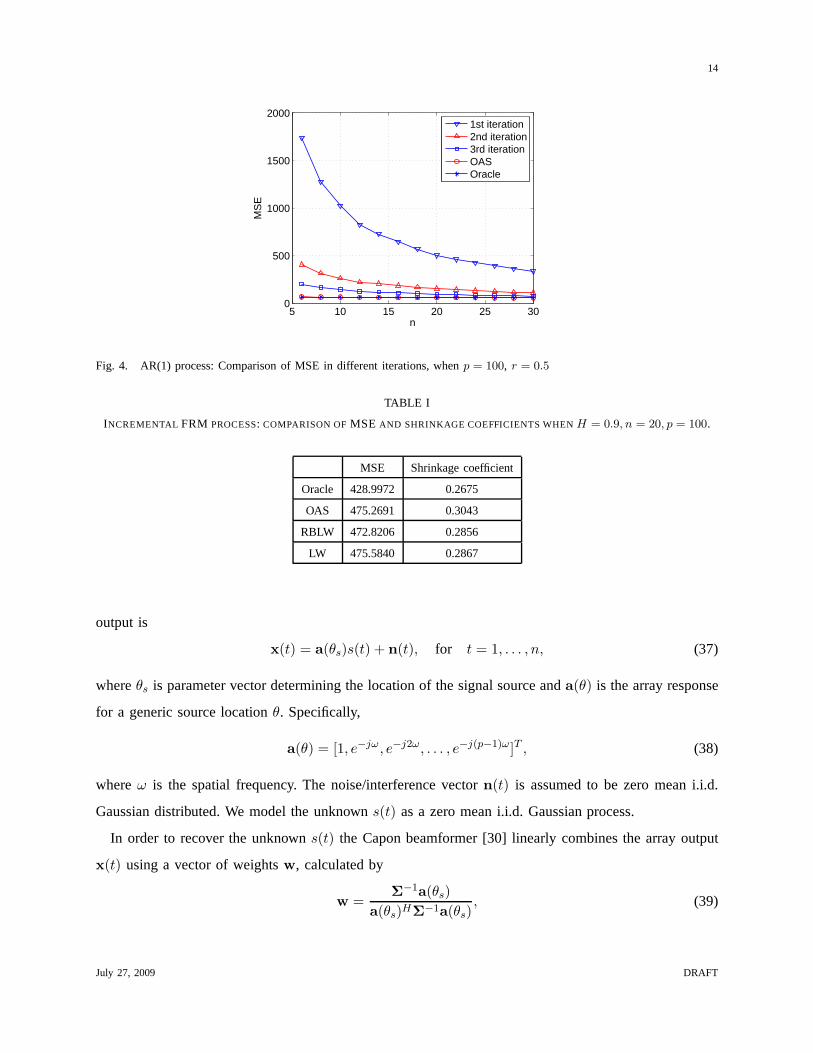
In Fig. 4 we plot the MSE of the first three iterations obtainedby the iterative procedure in (21) and

(20). For comparison we also plot the results of the OAS and the oracle estimator. We setr = 0.5 in

this example and start the iterations with the initial guessΣ0 = S. From Fig. 4 it can be seen that as the

iterations proceed, the MSE gradually decreases towards that of the OAS estimator, which is very close

to that of the oracle.

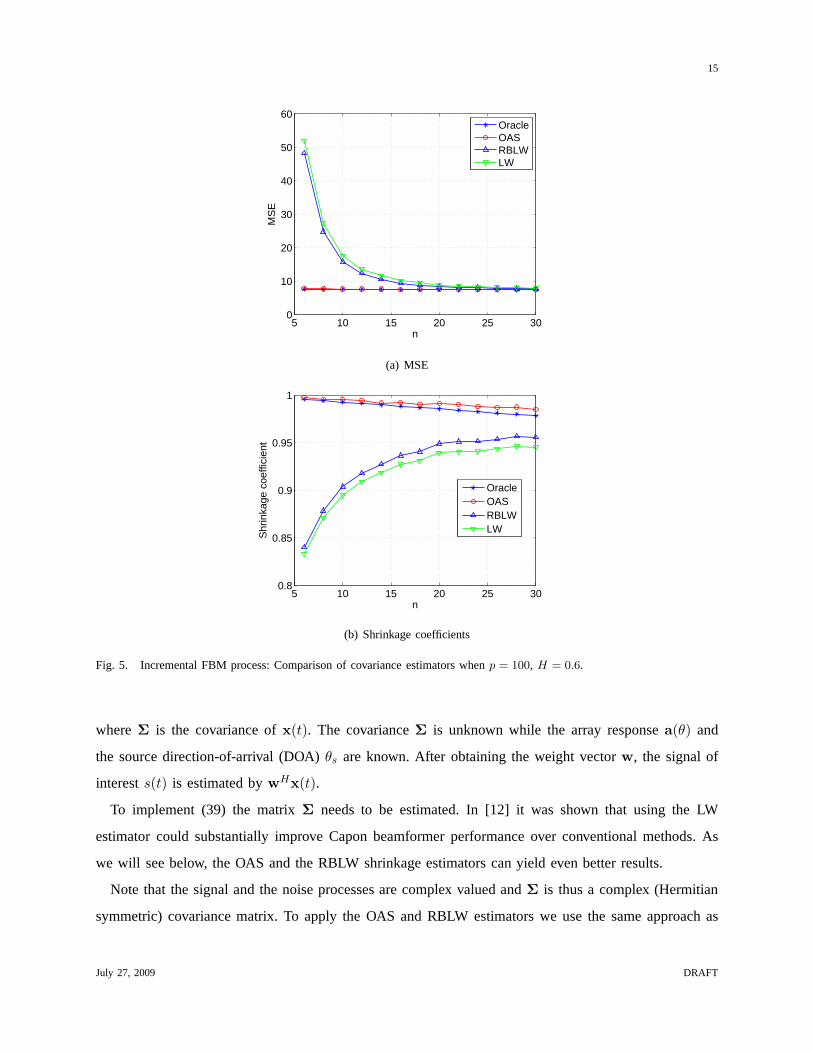
In the second experiment, we setΣ as the covariance matrix associated with the increment process of

fractional Brownian motion (FBM) exhibiting long-range dependence. Such processes are often used to

model internet traffic [29] and other complex phenomena. Theform of the covariance matrix is given by

Σij =1

2

[(|i − j| + 1)2H − 2|i − j|2H + (|i − j| − 1)2H

], (36)

July 27, 2009 DRAFT

11

5 10 15 20 25 300

10

20

30

40

50

n

MS

E

OracleOASRBLWLW

(a) MSE

5 10 15 20 25 300.8

0.85

0.9

0.95

1

n

Shr

inka

ge c

oeffi

cien

t

OracleOASRBLWLW

(b) Shrinkage coefficients

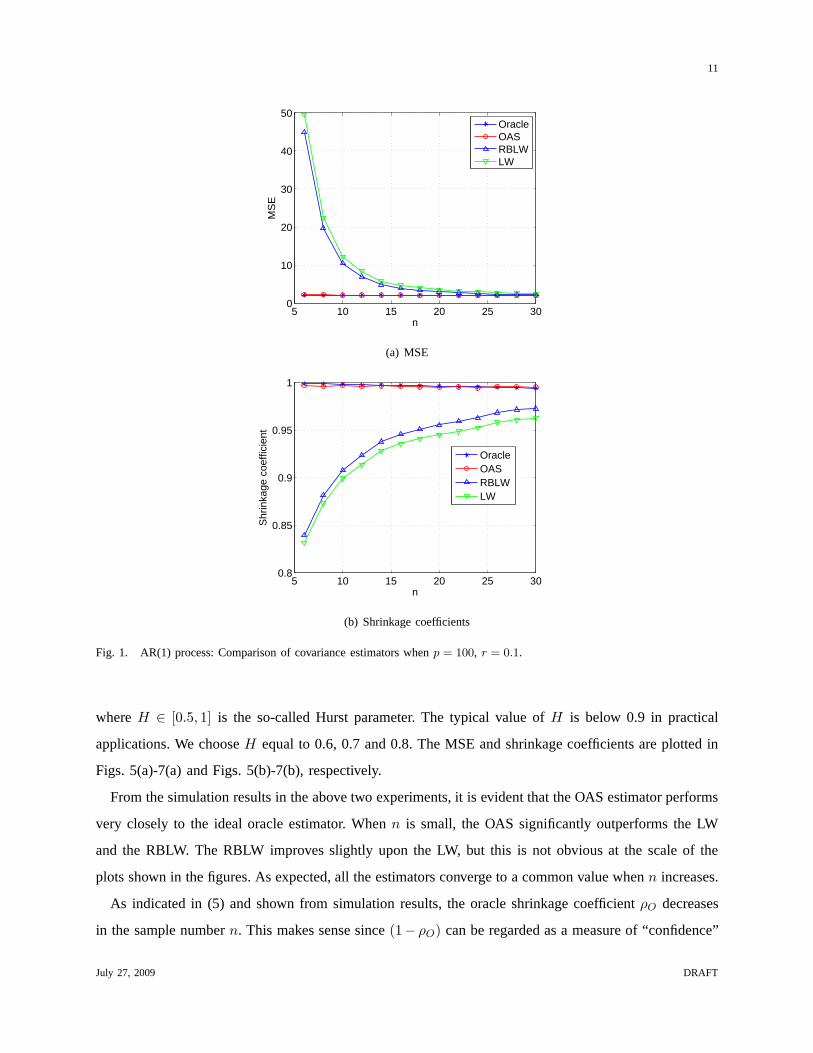
Fig. 1. AR(1) process: Comparison of covariance estimatorswhenp = 100, r = 0.1.

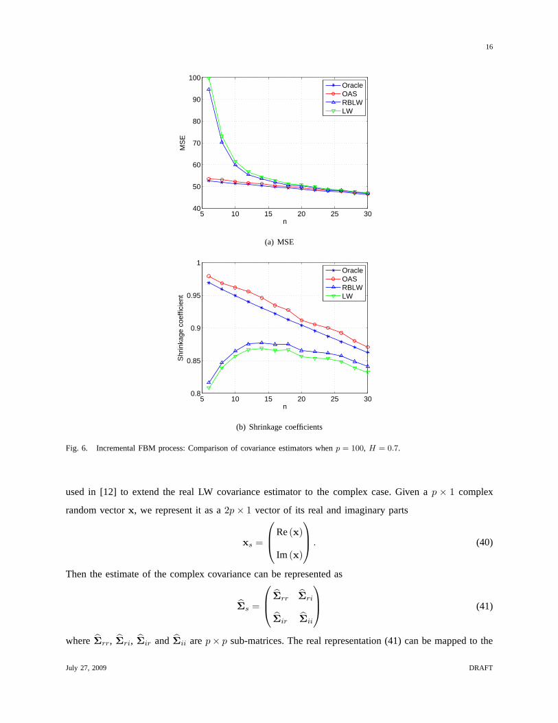
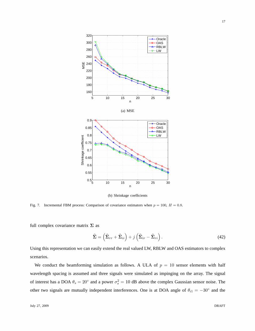
whereH ∈ [0.5, 1] is the so-called Hurst parameter. The typical value ofH is below 0.9 in practical

applications. We chooseH equal to 0.6, 0.7 and 0.8. The MSE and shrinkage coefficients are plotted in

Figs. 5(a)-7(a) and Figs. 5(b)-7(b), respectively.

From the simulation results in the above two experiments, itis evident that the OAS estimator performs

very closely to the ideal oracle estimator. Whenn is small, the OAS significantly outperforms the LW

and the RBLW. The RBLW improves slightly upon the LW, but thisis not obvious at the scale of the

plots shown in the figures. As expected, all the estimators converge to a common value whenn increases.

As indicated in (5) and shown from simulation results, the oracle shrinkage coefficientρO decreases

in the sample numbern. This makes sense since(1− ρO) can be regarded as a measure of “confidence”

July 27, 2009 DRAFT

12

5 10 15 20 25 3050

60

70

80

90

100

110

n

MS

E

OracleOASRBLWLW

(a) MSE

5 10 15 20 25 300.8

0.85

0.9

0.95

1

n

Shr

inka

ge c

oeffi

cien

t

OracleOASRBLWLW

(b) Shrinkage coefficients

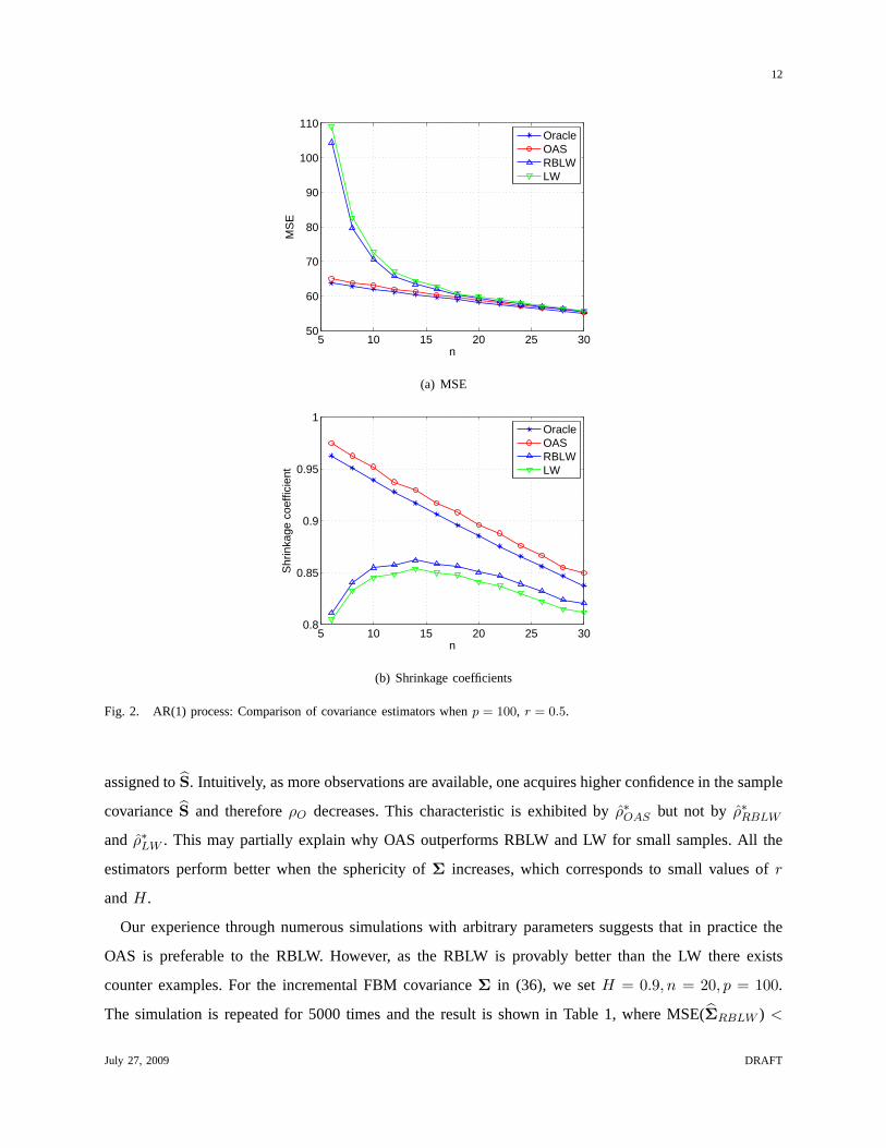
Fig. 2. AR(1) process: Comparison of covariance estimatorswhenp = 100, r = 0.5.

assigned toS. Intuitively, as more observations are available, one acquires higher confidence in the sample

covarianceS and thereforeρO decreases. This characteristic is exhibited byρ∗OAS but not by ρ∗RBLW

and ρ∗LW . This may partially explain why OAS outperforms RBLW and LW for small samples. All the

estimators perform better when the sphericity ofΣ increases, which corresponds to small values ofr

andH.

Our experience through numerous simulations with arbitrary parameters suggests that in practice the

OAS is preferable to the RBLW. However, as the RBLW is provably better than the LW there exists

counter examples. For the incremental FBM covarianceΣ in (36), we setH = 0.9, n = 20, p = 100.

The simulation is repeated for 5000 times and the result is shown in Table 1, where MSE(ΣRBLW ) <

July 27, 2009 DRAFT

13

5 10 15 20 25 30250

300

350

400

450

500

550

600

650

n

MS

E

OracleOASRBLWLW

(a) MSE

5 10 15 20 25 300.2

0.3

0.4

0.5

0.6

0.7

0.8

n

Shr

inka

ge c

oeffi

cien

t

OracleOASRBLWLW

(b) Shrinkage coefficients

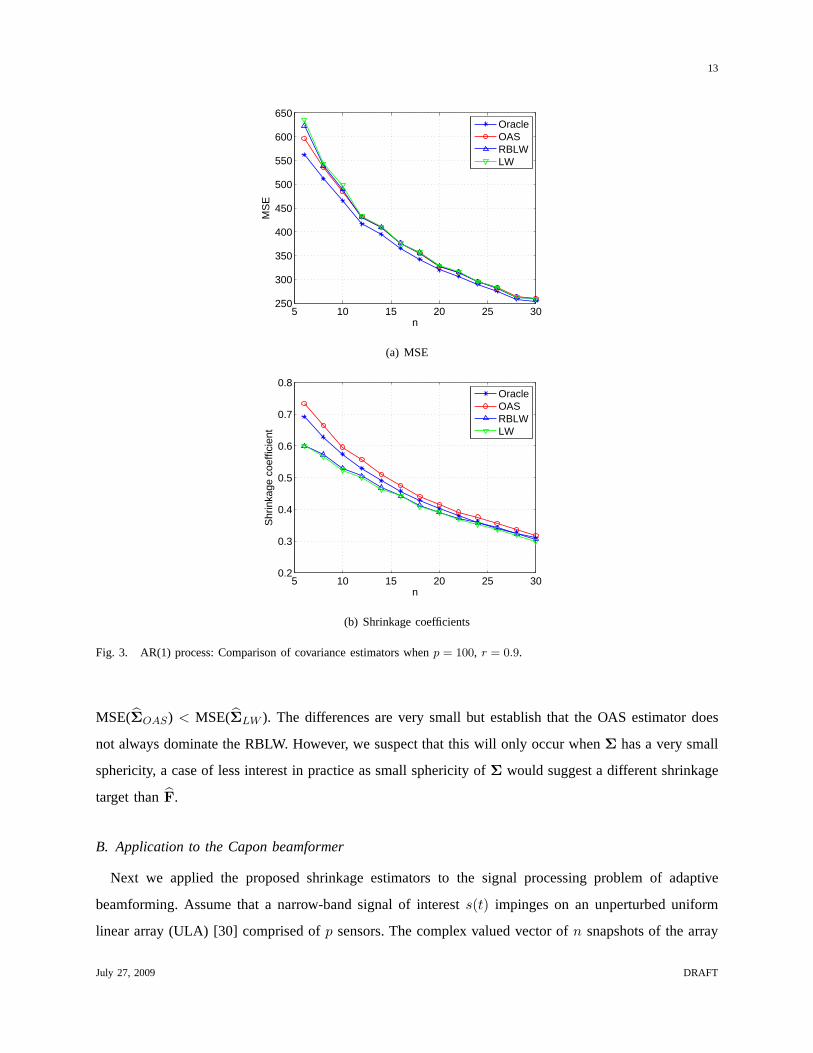
Fig. 3. AR(1) process: Comparison of covariance estimatorswhenp = 100, r = 0.9.

MSE(ΣOAS) < MSE(ΣLW ). The differences are very small but establish that the OAS estimator does

not always dominate the RBLW. However, we suspect that this will only occur whenΣ has a very small

sphericity, a case of less interest in practice as small sphericity of Σ would suggest a different shrinkage

target thanF.

B. Application to the Capon beamformer

Next we applied the proposed shrinkage estimators to the signal processing problem of adaptive

beamforming. Assume that a narrow-band signal of interests(t) impinges on an unperturbed uniform

linear array (ULA) [30] comprised ofp sensors. The complex valued vector ofn snapshots of the array

July 27, 2009 DRAFT

14

5 10 15 20 25 300

500

1000

1500

2000

n

MS

E

1st iteration2nd iteration3rd iterationOASOracle

Fig. 4. AR(1) process: Comparison of MSE in different iterations, whenp = 100, r = 0.5

TABLE I

INCREMENTAL FRM PROCESS: COMPARISON OFMSE AND SHRINKAGE COEFFICIENTS WHENH = 0.9, n = 20, p = 100.

MSE Shrinkage coefficient

Oracle 428.9972 0.2675

OAS 475.2691 0.3043

RBLW 472.8206 0.2856

LW 475.5840 0.2867

output is

x(t) = a(θs)s(t) + n(t), for t = 1, . . . , n, (37)

whereθs is parameter vector determining the location of the signal source anda(θ) is the array response

for a generic source locationθ. Specifically,

a(θ) = [1, e−jω, e−j2ω, . . . , e−j(p−1)ω]T , (38)

whereω is the spatial frequency. The noise/interference vectorn(t) is assumed to be zero mean i.i.d.

Gaussian distributed. We model the unknowns(t) as a zero mean i.i.d. Gaussian process.

In order to recover the unknowns(t) the Capon beamformer [30] linearly combines the array output

x(t) using a vector of weightsw, calculated by

w =Σ−1a(θs)

a(θs)HΣ−1a(θs), (39)

July 27, 2009 DRAFT

15

5 10 15 20 25 300

10

20

30

40

50

60

n

MS

E

OracleOASRBLWLW

(a) MSE

5 10 15 20 25 300.8

0.85

0.9

0.95

1

n

Shr

inka

ge c

oeffi

cien

t

OracleOASRBLWLW

(b) Shrinkage coefficients

Fig. 5. Incremental FBM process: Comparison of covariance estimators whenp = 100, H = 0.6.

whereΣ is the covariance ofx(t). The covarianceΣ is unknown while the array responsea(θ) and

the source direction-of-arrival (DOA)θs are known. After obtaining the weight vectorw, the signal of

interests(t) is estimated bywHx(t).

To implement (39) the matrixΣ needs to be estimated. In [12] it was shown that using the LW

estimator could substantially improve Capon beamformer performance over conventional methods. As

we will see below, the OAS and the RBLW shrinkage estimators can yield even better results.

Note that the signal and the noise processes are complex valued andΣ is thus a complex (Hermitian

symmetric) covariance matrix. To apply the OAS and RBLW estimators we use the same approach as

July 27, 2009 DRAFT

16

5 10 15 20 25 3040

50

60

70

80

90

100

n

MS

E

OracleOASRBLWLW

(a) MSE

5 10 15 20 25 300.8

0.85

0.9

0.95

1

n

Shr

inka

ge c

oeffi

cien

t

OracleOASRBLWLW

(b) Shrinkage coefficients

Fig. 6. Incremental FBM process: Comparison of covariance estimators whenp = 100, H = 0.7.

used in [12] to extend the real LW covariance estimator to thecomplex case. Given ap × 1 complex

random vectorx, we represent it as a2p × 1 vector of its real and imaginary parts

xs =

Re(x)

Im (x)

. (40)

Then the estimate of the complex covariance can be represented as

Σs =

Σrr Σri

Σir Σii

(41)

whereΣrr, Σri, Σir andΣii arep× p sub-matrices. The real representation (41) can be mapped tothe

July 27, 2009 DRAFT

17

5 10 15 20 25 30

160

180

200

220

240

260

280

300

320

n

MS

E

OracleOASRBLWLW

(a) MSE

5 10 15 20 25 300.5

0.55

0.6

0.65

0.7

0.75

0.8

0.85

0.9

n

Shr

inka

ge c

oeffi

cien

t

OracleOASRBLWLW

(b) Shrinkage coefficients

Fig. 7. Incremental FBM process: Comparison of covariance estimators whenp = 100, H = 0.8.

full complex covariance matrixΣ as

Σ =(Σrr + Σii

)+ j

(Σir − Σri

). (42)

Using this representation we can easily extend the real valued LW, RBLW and OAS estimators to complex

scenarios.

We conduct the beamforming simulation as follows. A ULA ofp = 10 sensor elements with half

wavelength spacing is assumed and three signals were simulated as impinging on the array. The signal

of interest has a DOAθs = 20◦ and a powerσ2s = 10 dB above the complex Gaussian sensor noise. The

other two signals are mutually independent interferences.One is at DOA angle ofθi1 = −30◦ and the

July 27, 2009 DRAFT

18

10 20 30 40 50 609

10

11

12

13

14

15

n

SIN

R (

dB)

LWOASRBLW

Fig. 8. Comparison between different covariance shrinkageestimators in the Capon beamformer. SINR is plotted versus number

of snapshotsn. OAS achieves as much as 1 dB improvement over the LW.

other one is close to the source of interest with its angular location corresponding to a spatial frequency

of

ωi2 = π sin(θs) + 2πγ

p

whereγ is set to 0.9. Each signal has power 15 dB above the sensor noise.

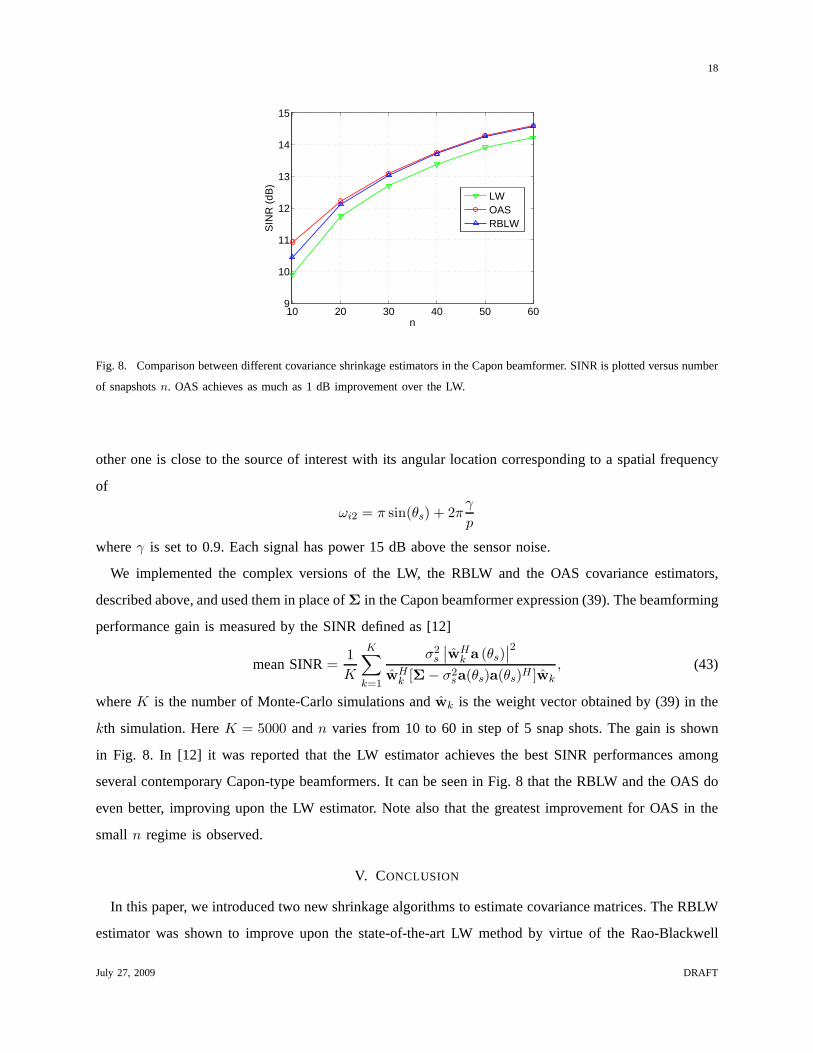
We implemented the complex versions of the LW, the RBLW and the OAS covariance estimators,

described above, and used them in place ofΣ in the Capon beamformer expression (39). The beamforming

performance gain is measured by the SINR defined as [12]

mean SINR=1

K

K∑

k=1

σ2s

∣∣wHk a (θs)

∣∣2

wHk [Σ − σ2

sa(θs)a(θs)H ]wk, (43)

whereK is the number of Monte-Carlo simulations andwk is the weight vector obtained by (39) in the

kth simulation. HereK = 5000 andn varies from 10 to 60 in step of 5 snap shots. The gain is shown

in Fig. 8. In [12] it was reported that the LW estimator achieves the best SINR performances among

several contemporary Capon-type beamformers. It can be seen in Fig. 8 that the RBLW and the OAS do

even better, improving upon the LW estimator. Note also thatthe greatest improvement for OAS in the

small n regime is observed.

V. CONCLUSION

In this paper, we introduced two new shrinkage algorithms toestimate covariance matrices. The RBLW

estimator was shown to improve upon the state-of-the-art LWmethod by virtue of the Rao-Blackwell

July 27, 2009 DRAFT

19

theorem. The OAS estimator was developed by iterating on theoptimal oracle estimate, where the limiting

form was determined analytically. The RBLW provably dominates the LW, and the OAS empirically

outperforms both the RBLW and the LW in most experiments we have conducted. The proposed OAS

and RBLW estimators have simple explicit expressions and are easy to implement. Furthermore, they

share similar structure differing only in the form of the shrinkage coefficients. We applied these estimators

to the Capon beamformer and obtained significant gains in performance as compared to the LW Capon

beamformer implementation.

Through out the paper we set the shrinkage target as the scaled identity matrix. The theory developed

here can be extended to other non-identity shrinkage targets. An interesting question for future research

is how to choose appropriate targets in specific applications.

VI. A PPENDIX

In this appendix we prove Theorem 2. Theorem 2 is non-trivialand requires careful treatment using

results from the theory of Haar measure and singular Wishartdistributions. The proof will require several

intermediate results stated as lemmas. We begin with a definition.

Definition 1. Let {xi}ni=1 be a sample ofp-dimensional i.i.d. Gaussian vectors with mean zero and

covarianceΣ. Define ap × n matrix X as

X = (x1,x2, . . . ,xn) . (44)

Denoter = min(p, n) and define the singular value decomposition onX as

X = HΛQ, (45)

whereH is a p× r matrix such thatHTH = I, Λ is a r× r diagonal matrix in probability 1, comprised

of the singular values ofX, andQ is a r × n matrix such thatQQT = I.

Next we state and prove three lemmas.

Lemma 1. Let (H,Λ,Q) be matrices defined in Definition 1. ThenQ is independent ofH and Λ.

Proof: For the casen ≤ p, H is a p × n matrix, Λ is a n × n square diagonal matrix andQ is a

n × n orthogonal matrix. The pdf ofX is

p (X) =1

(2π)pn/2det(Σ)n/2e−

1

2Tr(XXT Σ−1). (46)

July 27, 2009 DRAFT

20

SinceXXT = HΛΛT HT , the joint pdf of(H,Λ,Q) is

p (H,Λ,Q) =

1

(2π)pn/2det(Σ)n/2e−

1

2Tr(HΛΛT HT Σ−1)J (X → H,Λ,Q) ,

(47)

whereJ (X → H,Λ,Q) is the Jacobian converting fromX to (H,Λ,Q). According to Lemma 2.4 of

[21],

J (X → H,Λ,Q) =

2−ndet(Λ)p−nn∏

j<k

(λ2

j − λ2k

)gn,p (H) gn,n (Q) ,

(48)

whereλj denotes thej-th diagonal element ofΛ and gn,p(H) andgn,n(Q) are functions ofH andQ

defined in [21].

Substituting (48) into (47),p (H,Λ,Q) can be factorized into functions of(H,Λ) andQ. Therefore,

Q is independent ofH andΛ.

Similarly, one can show thatQ is independent ofH andΛ whenn > p.

Lemma 2. Let Q be a matrix defined in Definition 1. Denoteq as an arbitrary column vector ofQ and

qj as thej-th element ofq. Then

E{q4j

}=

3

n(n + 2)(49)

and

E{q2kq

2j

}=

1

n(n + 2), k 6= j. (50)

Proof: The proof is different for the cases thatn ≤ p andn > p, which are treated separately.

(1) Casen ≤ p:

In this case,Q is a real Haar matrix and is isotropically distributed [22],[24], [25], i.e., for any unitary

matricesΦ andΨ which are independent withQ, ΦQ andQΨ have the same pdf ofQ:

p(ΦQ) = p(QΨ) = p(Q). (51)

Following [23] in the complex case, we now use (51) to calculate the fourth order moments of elements

of Q. SinceQ and

cos θ sin θ

− sin θ cos θ

1

. . .

1

Q

July 27, 2009 DRAFT

21

are also identically distributed, we have

E{Q4

11

}

= E{

(Q11 cos θ + Q21 sin θ)4}

= cos4 θE{Q4

11

}+ sin4 θE

{Q4

22

}

+ 6cos2 θ sin2 θE{Q2

11Q221

}

+ 2cos3 θ sin θE{Q3

11Q21

}+ 2cos θ sin3 θE

{Q11Q

321

}

(52)

By taking θ = −θ in (52), it is easy to see that

2 cos3 θ sin θE{Q3

11Q21

}+ 2cos θ sin3 θE

{Q11Q

321

}= 0.

The elements of[Qii] are identically distributed. We thus haveE{Q4

11

}= E

{Q4

22

}, and hence

E{Q4

11

}

=(cos4 θ + sin4 θ

)E{Q4

11

}+ 6cos2 θ sin2 θE

{Q2

11Q221

}.

(53)

By taking θ = π/3,

E{Q4

11

}= 3E

{Q2

11Q221

}. (54)

Now we considerE

{(∑nj=1 Q2

j1

)2}

. SinceQTQ = QQT = I,n∑

j=1Q2

j1 = 1. This implies

1 =n∑

j=1

E{Q4

j1

}+∑

j 6=k

E{Q2

j1Q2k1

}

= nE{Q4

11

}+ n(n − 1)E

{Q2

11Q221

}.

(55)

Substituting (54) into (55), we obtain that

E{Q4

11

}=

3

n(n + 2), (56)

and

E{Q2

11Q221

}=

1

n(n + 2). (57)

It is easy to see thatE{q4j

}= E

{Q4

11

}andE

{q2j q

2k

}= E

{Q2

11Q221

}. Therefore (49) and (50) are

proved for the case ofn ≤ p.

(2) Casen > p:

The pdf ofq can be obtained by Lemma 2.2 of [21]

p(q) = C1det(I− qqT

)(n−p−2)/2I(qqT ≺ I), (58)

July 27, 2009 DRAFT

22

where

C1 =π−p/2Γ{n/2}

Γ{(n − p)/2}, (59)

andI (·) is the indicator function specifying the support ofq. Eq. (58) indicates that the elements ofq

are identically distributed. Therefore,E{

q4j

}= E

[q41

}and E

{q2j q

2k

}= E

{q21q

22

}. By the definition

of expectation,

E{q41

}= C1

∫

qqT≺I

q41det

(I− qqT

)(n−p−2)/2dq, (60)

and

E{q21q

22

}= C1

∫

qqT≺I

q21q

22det

(I − qqT

)(n−p−2)/2dq. (61)

Noting that

qqT ≺ I ⇔ qTq < 1 (62)

and

det(I − qqT

)= 1 − qTq, (63)

we have

E{q41

}= C1

∫

qT q<1q41(1 − qTq)

1

2(n−p−2)dq

= C1

∫p

P

j=1

q2

j <1q41

1 −

p∑

j=1

q2j

1

2(n−p−2)

dq1 . . . dqp.

(64)

By changing variable of integration(q1, q2, · · · , qp) to (r, θ1, θ2, · · · , θp−1) such that

q1 = r cos θ1

q2 = r sin θ1 cos θ2

q3 = r sin θ1 sin θ2 cos θ3

......

qp−1 = r sin θ1 sin θ2 · · · sin θp−2 cos θp−1

qp = r sin θ1 sin θ2 · · · sin θp−2 sin θp−1

, (65)

we obtain

E{q41

}= C1

∫ π

0dθ1

∫ π

0dθ2 · · ·

∫ π

0dθp−2

∫ 2π

0dθp−1

·

∫ 1

0r4 cos4 θ1

(1 − r2

) 1

2(n−p−2)

∣∣∣∣∂ (q1, · · · , qp)

∂ (r, θ1, · · · , θp−1)

∣∣∣∣ dr,

(66)

where ∣∣∣∣∂ (q1, · · · , qp)

∂ (r, θ1, · · · , θp−1)

∣∣∣∣ = rp−1 sinp−2 θ1 sinp−3 θ2 · · · sin θp−2

July 27, 2009 DRAFT

23

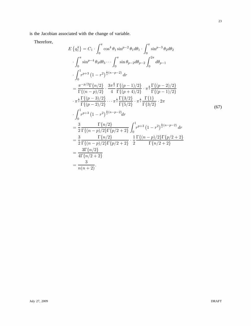
is the Jacobian associated with the change of variable.

Therefore,

E{q41

}= C1 ·

∫ π

0cos4 θ1 sinp−2 θ1dθ1 ·

∫ π

0sinp−3 θ2dθ2

·

∫ π

0sinp−4 θ3dθ3 · · ·

∫ π

0sin θp−2dθp−2

∫ 2π

0dθp−1

·

∫ 1

0rp+3

(1 − r2

) 1

2(n−p−2)

dr

=π−p/2Γ{n/2}

Γ{(n − p)/2}·3π

1

2

4

Γ{(p − 1)/2}

Γ{(p + 4)/2}· π

1

2

Γ{(p − 2)/2}

Γ{(p − 1)/2}

· π1

2

Γ{(p − 3)/2}

Γ{(p − 2)/2}· · · π

1

2

Γ{3/2}

Γ{5/2}· π

1

2

Γ{1}

Γ{3/2}· 2π

·

∫ 1

0rp+3

(1 − r2

) 1

2(n−p−2)

dr

=3

2

Γ{n/2}

Γ{(n − p)/2}Γ{p/2 + 2}

∫ 1

0rp+3

(1 − r2

) 1

2(n−p−2)

dr

=3

2

Γ{n/2}

Γ{(n − p)/2}Γ{p/2 + 2}·1

2

Γ{(n − p)/2}Γ{p/2 + 2}

Γ{n/2 + 2}

=3Γ{n/2}

4Γ{n/2 + 2}

=3

n(n + 2).

(67)

July 27, 2009 DRAFT

24

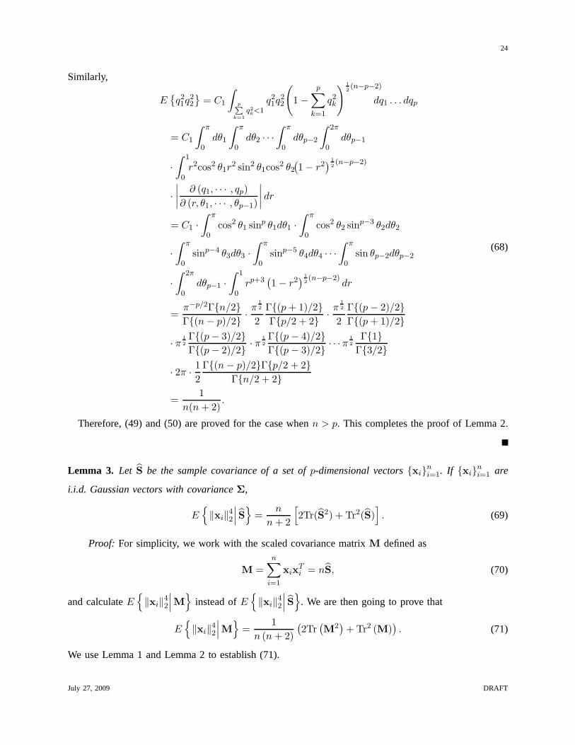
Similarly,

E{q21q

22

}= C1

∫p

P

k=1

q2

k<1q21q

22

(

1 −

p∑

k=1

q2k

) 1

2(n−p−2)

dq1 . . . dqp

= C1

∫ π

0dθ1

∫ π

0dθ2 · · ·

∫ π

0dθp−2

∫ 2π

0dθp−1

·

∫ 1

0r2cos2 θ1r

2 sin2 θ1cos2 θ2

(1 − r2

) 1

2(n−p−2)

·

∣∣∣∣∂ (q1, · · · , qp)

∂ (r, θ1, · · · , θp−1)

∣∣∣∣ dr

= C1 ·

∫ π

0cos2 θ1 sinp θ1dθ1 ·

∫ π

0cos2 θ2 sinp−3 θ2dθ2

·

∫ π

0sinp−4 θ3dθ3 ·

∫ π

0sinp−5 θ4dθ4 · · ·

∫ π

0sin θp−2dθp−2

·

∫ 2π

0dθp−1 ·

∫ 1

0rp+3

(1 − r2

) 1

2(n−p−2)

dr

=π−p/2Γ{n/2}

Γ{(n − p)/2}·π

1

2

2

Γ{(p + 1)/2}

Γ{p/2 + 2}·π

1

2

2

Γ{(p − 2)/2}

Γ{(p + 1)/2}

· π1

2

Γ{(p − 3)/2}

Γ{(p − 2)/2}· π

1

2

Γ{(p − 4)/2}

Γ{(p − 3)/2}· · · π

1

2

Γ{1}

Γ{3/2}

· 2π ·1

2

Γ{(n − p)/2}Γ{p/2 + 2}

Γ{n/2 + 2}

=1

n(n + 2).

(68)

Therefore, (49) and (50) are proved for the case whenn > p. This completes the proof of Lemma 2.

Lemma 3. Let S be the sample covariance of a set ofp-dimensional vectors{xi}ni=1. If {xi}

ni=1 are

i.i.d. Gaussian vectors with covarianceΣ,

E{‖xi‖

42

∣∣∣ S}

=n

n + 2

[2Tr(S2) + Tr2(S)

]. (69)

Proof: For simplicity, we work with the scaled covariance matrixM defined as

M =

n∑

i=1

xixTi = nS, (70)

and calculateE{‖xi‖

42

∣∣∣M}

instead ofE{‖xi‖

42

∣∣∣ S}

. We are then going to prove that

E{‖xi‖

42

∣∣∣M}

=1

n (n + 2)

(2Tr

(M2)

+ Tr2 (M)). (71)

We use Lemma 1 and Lemma 2 to establish (71).

July 27, 2009 DRAFT

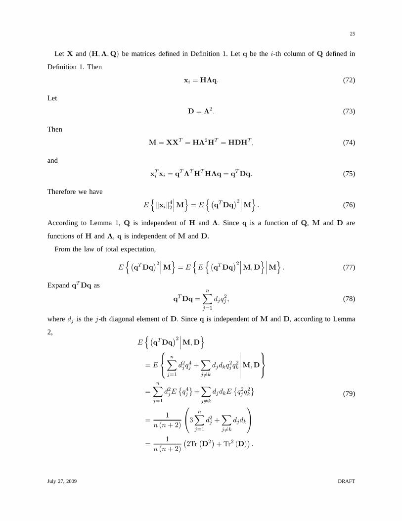
25

Let X and (H,Λ,Q) be matrices defined in Definition 1. Letq be thei-th column ofQ defined in

Definition 1. Then

xi = HΛq. (72)

Let

D = Λ2. (73)

Then

M = XXT = HΛ2HT = HDHT , (74)

and

xTi xi = qTΛTHTHΛq = qT Dq. (75)

Therefore we have

E{‖xi‖

42

∣∣∣M}

= E{(

qTDq)2∣∣∣M

}. (76)

According to Lemma 1,Q is independent ofH and Λ. Sinceq is a function ofQ, M and D are

functions ofH andΛ, q is independent ofM andD.

From the law of total expectation,

E{(

qTDq)2∣∣∣M

}= E

{E{(

qTDq)2∣∣∣M,D

}∣∣∣M}

. (77)

ExpandqTDq as

qTDq =

n∑

j=1

djq2j , (78)

wheredj is thej-th diagonal element ofD. Sinceq is independent ofM andD, according to Lemma

2,

E{(

qTDq)2∣∣∣M,D

}

= E

n∑

j=1

d2jq

4j +

∑

j 6=k

djdkq2j q

2k

∣∣∣∣∣∣M,D

=

n∑

j=1

d2jE{q4j

}+∑

j 6=k

djdkE{q2j q

2k

}

=1

n (n + 2)

3n∑

j=1

d2j +

∑

j 6=k

djdk

=1

n (n + 2)

(2Tr

(D2)

+ Tr2 (D)).

(79)

July 27, 2009 DRAFT

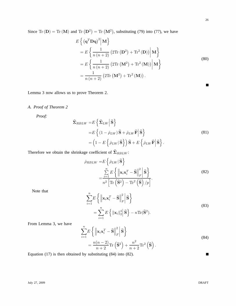
26

SinceTr (D) = Tr (M) andTr(D2)

= Tr(M2), substituting (79) into (77), we have

E{(

qT Dq)2∣∣∣M

}

= E

{1

n (n + 2)

(2Tr

(D2)

+ Tr2 (D))∣∣∣∣M

}

= E

{1

n (n + 2)

(2Tr

(M2)

+ Tr2 (M))∣∣∣∣M

}

=1

n (n + 2)

(2Tr

(M2)

+ Tr2 (M)).

(80)

Lemma 3 now allows us to prove Theorem 2.

A. Proof of Theorem 2

Proof:

ΣRBLW =E{

ΣLW

∣∣∣ S}

=E{

(1 − ρLW ) S + ρLW F

∣∣∣ S}

=(1 − E

{ρLW | S

})S + E

{ρLW F

∣∣∣ S}

.

(81)

Therefore we obtain the shrinkage coefficient ofΣRBLW :

ρRBLW =E{

ρLW | S}

=

n∑i=1

E

{∥∥∥xixTi − S

∥∥∥2

F

∣∣∣∣ S}

n2[Tr(S2)− Tr2

(S)

/p] .

(82)

Note thatn∑

i=1

E

{∥∥∥xixTi − S

∥∥∥2

F

∣∣∣∣ S}

=

n∑

i=1

E{‖xi‖

42

∣∣∣ S}− nTr(S2).

(83)

From Lemma 3, we haven∑

i=1

E

{∥∥∥xixTi − S

∥∥∥2

F

∣∣∣∣ S}

=n(n − 2)

n + 2Tr(S2)

+n2

n + 2Tr2

(S)

.

(84)

Equation (17) is then obtained by substituting (84) into (82).

July 27, 2009 DRAFT

27

REFERENCES

[1] C. Stein, “Inadmissibility of the usual estimator for the mean of a multivariate distribution,”Proc. Third Berkeley Symp.

Math. Statist. Prob. 1, pp. 197-206, 1956.

[2] W. James and C. Stein, “Estimation with quadratic loss,”Proceedings of the 4th Berkeley Symposium on Mathematical

Statistics and Probability, Berkeley, CA, vol. 1, page 361-379, University of California Press, 1961.

[3] C. Stein, “Estimation of a covariance matrix,” InRietz Lecture, 39th Annual Meeting, IMS, Atlanta, GA, 1975.

[4] L. R. Haff, “Empirical Bayes Estimation of the Multivariate Normal Covariance Matrix,”Annals of Statistics, vol. 8, no. 3,

pp. 586-597, 1980.

[5] D. K. Dey and C. Srinivasan, “Estimation of a covariance matrix under Stein’s loss,”Annals of Statistics, vol. 13, pp.

1581-1591, 1985.

[6] R. Yang, J. O. Berger, “Estimation of a covariance matrixusing the reference prior,”Annals of Statistics, vol. 22, pp.

1195-1211, 1994.

[7] O. Ledoit, M. Wolf, “Improved estimation of the covariance matrix of stock returns with an application to portfolio selection,”

Journal of Empirical Finance, vol. 10, no. 5, pp. 603-621, Dec. 2003.

[8] O. Ledoit and M. Wolf, “A well-conditioned estimator forlarge-dimensional covariance matrices,”Journal of Multivariate

Analysis, vol. 88, no. 2, pp. 365-411, Feb. 2004.

[9] O. Ledoit, M. Wolf, “Honey, I Shrunk the Sample Covariance Matrix,” Journal of Portfolio Management, vol. 31, no. 1,

2004.

[10] P. Bickel, E. Levina, “Regularized estimation of largecovariance matrices,”Annals of Statistics, vol. 36, pp. 199-227,

2008.

[11] Y. C. Eldar and J. Chernoi, “A Pre-Test Like Estimator Dominating the Least-Squares Method,”Journal of Statistical

Planning and Inference, vol. 138, no. 10, pp. 3069-3085, 2008.

[12] R. Abrahamsson, Y. Selen and P. Stoica, “Enhanced covariance matrix estimators in adaptive beamforming,”IEEE Proc.

of ICASSP, pp. 969-972, 2007.

[13] P. Stoica, J. Li, X. Zhu and J. Guerci, “On using a priori knowledge in space-time adaptive processing,”IEEE Trans.

Signal Process., vol. 56, pp. 2598-2602, 2008.

[14] J. Li, L. Du and P. Stoica, “Fully automatic computationof diagonal loading levels for robust adaptive beamforming,”

IEEE Proc. of ICASSP, pp. 2325-2328, 2008.

[15] P. Stoica, J. Li, T. Xing, “On Spatial Power Spectrum andSignal Estimation Using the Pisarenko Framework,”IEEE Trans.

Signal Process., vol. 56, pp. 5109-5119, 2008.

[16] Y. I. Abramovich and B. A. Johnson, “GLRT-Based Detection-Estimation for Undersampled Training Conditions,”IEEE

Trans. Signal Process., vol. 56, no. 8, pp. 3600-3612, Aug. 2008.

[17] J. Schafer and K. Strimmer, “A Shrinkage approach to large-scale covariance matrix estimation and implications for

functional genomics,”Statistical Applications in Genetics and Molecular Biology, vol. 4, no. 1, 2005.

[18] S. Johh, “Some optimal multivariate tests,”Biometrika, vol. 58, pp. 123-127, 1971.

[19] M. S. Srivastava and C. G. Khatri,An introduction to multivariate statistics, 1979.

[20] O. Ledoit and M. Wolf, “Some Hypothesis Tests for the Covariance Matrix When the Dimension Is Large Compared to

the Sample Size,”Annals of Statistics, vol. 30, no. 4, pp. 1081-1102, Aug. 2002.

[21] M. S. Srivastava, “Singular Wishart and multivariate beta distributions,”Annals of Statistics, vol. 31, no. 5, pp. 1537-1560,

2003.

July 27, 2009 DRAFT

28

[22] B. Hassibi and T. L. Marzetta,“Multiple-antennas and isotropically random unitary inputs: the received signal density in

closed form,”IEEE Trans. Inf. Theory, vol. 48, no. 6, pp. 1473-1484, Jun. 2002.

[23] F. Hiai and D. Petz, “Asymptotic freeness almost everywhere for random matrices,”Acta Sci. Math. Szeged, vol. 66, pp.

801C826, 2000.

[24] T. L. Marzetta and B. M. Hochwald, “Capacity of a mobile multipleantenna communication link in Rayleigh flat fading,”

IEEE Trans. Inf. Theory, vol. 45, no. 1, pp. 139-157, 1999.

[25] Y. C. Eldar and S. Shamai, “A covariance shaping framework for linear multiuser detection,”IEEE Trans. Inf. Theory, vol.

51, no. 7, pp. 2426-2446, 2005.

[26] R. K. Mallik, “The pseudo-Wishart distribution and itsapplication to MIMO systems,”IEEE Trans. Inf. Theory, vol. 49,

pp. 2761-2769, Oct. 2003.

[27] G. Letac and H. Massam, “All invariant moments of the Wishart distribution,”Scand. J. Statist., vol. 31, no. 2, pp. 285-318,

2004.

[28] T. Bodnar and Y. Okhrin, “Properties of the singular, inverse and generalized inverse partitioned Wishart distributions,”

Journal of Multivariate Analysis, vol. 99, no. 10, pp. 2389-2405, Nov. 2008.

[29] W. E. Leland, M.S. Taqqu, W. Willinger and D.V.,Wilson,“On the self-similar nature of Ethernet traffic,”IEEE Trans.

Networking, vol. 2, pp. 1-15, 1994.

[30] P. Stoica and R. Moses,Spectral Analysis of Signals, Prentice Hall, Upper Saddle River, NJ, 2005.

[31] H. L. Van Trees,Detection, Estimation, and Modulation Theory, Part I, New York, NY: John Wiley & Sons, Inc., 1971.

[32] S. M. Pandit and S. Wu,Time Series and System Analysis with Applications, John Wiley & Sons, Inc., 1983.

July 27, 2009 DRAFT