AO-A097 4b ZOAUV IWACT DVO EUCTOA PCOLGFV/1EXPERIMENTAL STUDIES OF CADA-BASED UTILITY ASSESSMENT PROCEDUEECFEB 81 M R NOVICK, N J TURNER, L R NOVICKE N 501 4_77_C _048

UNCLASSIFIED TR-81- NL

MhEEOMOEEsooEEn

EomhhmhEEmhEEEI I

1326IIHI ,_ -

* 11.25 1=

MICROCOPY RESOLUTION TEST CHARTNATIONAL BUREAU OF STANDARDS-1963-A

" ~ ~TE:c, c.. REecw 81-2 ,

FEW,~ 1981m O2LEVEL

EiiEID Iwe4TAL S IIMES OF CA BA

UTILI1Y ASSE W PROXE

MELVIN R. NoviCK, NANCY J. TuRo, AND LAuRA R. NovICK

THE UtivERsrY oF Iom

S0

REPORT PREPARED UNDER OFFICE OF NAVAL RESEAC

coNPACT A0O1 77-C-(28MELVIN R.. Nticy, PRINCIPAL INVeSIGATO

THE NVSERsiTY OF ImA

IOM CITY., IOW

APPRIEI) FOR PUBLIC RELEASEJ DISTRIBUTION UNLIMITEDREPRDUCTION IN %*OLE OR IN PART IS PERITTED FORANY PURPOSE Or THE UNITED STATES GOVBWteeT, DTIC

S ELECTEAPR8 1981U

:s D

814 7D001

Unclassified49CURITy CLASSIFICATION OF THIS v AC (When Dom Efnion.

REPORT DOCUMENTATION PAGE _________________MOM

1. REPORT NMBERC 2. 'GOVT ACCESSION NO. S. 0*CIP1EN'tS CATAL OI UU69R

Technical Report 81-2 ,' YA W r 1 -6( Exerimental Studies of CADA-Based itt7 Rearch - pt.e4* 't Assessment Proceduresl............ Ja91- ec

Mevi 0 (Novick Nancy J.Turner and I

rPERFORMING ORGANIZATION "AMCK AND ADDRESS Ao AlS NU TS

University of Iowa 6215 31. U 02-04;3R04Division of Edulcational Psychology/ 04-1; 3N; 1504-04;R02Iowa City, Iowa 52242 04-01; NR 150-404______

11. CONTROLLING OFFICE NAME AND ADDRESS -I.15

Personnel and Training Research Program Fb ph8wlOffice of Naval Research (Code 458) 4.MJ911O AU

Arlington, VA 22217 6314. N IHG LACY-M AKLAL A009SS(it differmnt keg. Cerefln Office) 1S. SECURITY CLASS. &WE 1Me apeft)

(~Rq5UnclassifiedR P, 6IS&. IfrICATIOWN5RADING

Approved for public release, distribution unlimited

17. OISTRIISUY)ION STATEMENT (of the abeakact 001ten MOM Sle 81111.R if X40900be R

1S. SUPPLEMENTARY NOTES

19. KEY WORDS (Camntiu on~ l*ee side Ifne6eecceaO ad m.,i* IW Wleek R.emhe)

Utility Assessment Coherence, fixed-state assessment, regional coherence,local coherence, CADA, certainty effect, anchoring effect

P. LITRACT (Centhm an revo aids It 0000000Y M m & &FnN~ ak Ambe)'everal experiments were performed to investigate the degree of incoherenceassociated with, and the extent of biases caused by, the zert&Btyand&flcts for the following utility assessment procedures: staIdagsu1e fstate (wthout and with overfitting and least squares incoherence resolution),regional coherence, and local coherence. Several elicitation formsts were alsocompared. The purpose of these experiments was to assist in the developmet ofa reliable (coherent), bias-free, CAM-based method of utility assessment forgeneral use in educational evaluation.L

DOIF* M EDITION OF I Nov *Sa isSCLTJ\ Unclsiid 1i.D JAN 73 S/W 0102.LF-0401 _14IOIe

SCUONTY MS GIAIM Of0M A

Assaw Vs For January 30, 1981

unanumee . .0EXPERIMENTAL STUDIES OF CADA-IMAED

UTILITY ASSESSMENT PROCEDURES

Distribution/ Melvin R. NovickAvailability Codes

vail and/or Nancy 3. TurnerDist SpecialI

Laura R. Novick

The University of Iowa

Several experiments were performed to investigate thedegree of incoherence associated with, and the extent ofbiases caused by, the certainty and anchorint effects forthe following utility assessment procedures: standardgamble fixed state (without and with overfitting and leastsquares incoherence resolution), regional coherence, andlocal coherence. Several elicitation formats were alsocompared. The purpose of these experiments was to assistin the development of a reliable (coherent), bias-free,CADA-based method of utility assessment for general usein educational evaluation.

Utility assessment can be treated as a topic in the classical

psychometric specialty of scaling (e.g., Torgersen, 1958) or more

formally as part of a theory of measurement (Krantz, Luce, Suppes,

and Tversky, 1971). Novick and Lindley (1978, 1979) have dealt

with the use of uLility functions for applications in education and

have advocated the use of iho standard gamble (von Neumann and

Mlorgenscern, 1953) elicitation procedure with the addition of

coherence checking using overspecification and a least squares fit.

In this procedure utilities are inferred from probability judgments

offered by assessors.

'This research was supported under Contract N100014-77-C-0428

between the Office of Naval Research and The University of lowa.Opinions expressed herein are those of the authors and do not neces-sarily reflect those of the contracting agencies. The computer programdevelopment of David Libby and the consultative assistance of DavidChuang are gratefully acknowledged.

-2-I. w ~ I

Zarlier approaches to utility assessment (Mosteller and Noges,

1951; Schleifer, 1959, 1971; Raiff& and Schleifer, 1961; Keeney and

Raiff&, 1976; and so on) have been based on the use of fixed probe-

bility assessment procedures in which utilities are elicited directly.

It has been suggested (Mosteller and Nogee, 1951) that such pro-

cedures are easier to use because subjects are generally more familiar

with the quantity for which the utility funcion is desired than thy

are with probabilities. Since use of an easier procedure does not necessarily

insure that subject's responses will be coherent, an opportunity for

incoherence resolution is needed. However, the nature of the fixed

probability gambles makes it very difficult to check for coherence of

responses.

Although It was originally thought that utility theory would prove

useful as a descriptive model (Swalm, 1966, etc.), much criticism has

recently been levied against the use of utility theory in that capacity

(Coombs, 1975; Kahneman and Tversky, 1979). As principal critics,

Kahneman and Tversky have proposed an alternative descriptive model.

The ain basis for their criticism is that the phenomenon described by

Tversky (1977) as the certainty effect results in preferences that

violate the substitution axiom or expected utility hypothesis of

utility theory. This axiom (hypothesis) states that preference order is

invariant over probability mixtures and is formally equivalent to the

assumption that there is no positive or negative utility for the act of

gambling itself. Specifically, the certainty effect is the phenomenon

that the utility of an outcome seems greater when it is certain than

when it Is uncertain. This effect can be observed when subjects are

presented with a choice between a for-sure and a chance option, the choice

presented in the standard gamble, regional coherence, aed local

coherence assessment procedures discussed below.

-3-

Although utility theory is considered here as a normative model

-Tather than as a descriptive model, it Is still important to con-

aider the certainty effect. Tversky (1977) has shown that

even when subjects were told that their preferences violated uti-

lity theory, they were not inclined to change them (see also

Kahnemmn and Tversky, 1972). This brings into question the relia-

bility (coherence) and bias-free character of utility assesment

procedures and the value of those procedures in helping decision makers

be more coherent. However, two additional comments msot be made.

Whereas the gambles studied by Kahneman and Tversky involved gains

and losses from some undefined reference point, those studied by

Novick and Lindley considered passage to and from well-defined states.

Furthermore, the latter authors also included incoherence resolu-

tion as a part of their utility assessment procedure.

In another paper, Tversky and Kahneman (1974) described several

heuristics used by persons in assessing probabilities and the biases

to which they could lead. Of particular interest is the anchoring

and adJustment heuristic, whereby

the most readily available piece of information often forms an initial

basis for formulating responses, from which subsequent responses are

then adjusted. Since adjustments from this basis are often insufficient,

a central bias results. According to Slovic (1972), the anchoring and

adjustment heuristic is a natural strategy for easing the strain of

integrating information. The anchor serves as a register in which one

stores first Impressions or the results of earlier calculations. Slavic

-4-

advances two hypotheses to explain why adjustments from the anchor

are usually insufficient. First, people may stop adjusting too soon

because they tire of the mental effort involved in adjusting.

Alternatively, the anchor may take on a special salience,

causing people to feel that there is less risk in making estimates

close to it than in making estimates far from it.

In revieving the role of man-machine systems in decision ana-

lysis, Slovic, Fischhoff. and Lichtenstein (1977) suggested that

human factors such as the ways In which variations in instructions

or informational displays affect people's performance should be

studied in more detail. Some progress has been made in this area

with the finding that questions of complexity and representativeness

of material seem to have substantial effect on assessors' responses

(Fischhoff, Slovic, and LichLcnstein, 1977; Vlek, 1973). The study

of such factors might lead to an assessment procedure that minimizes

the Judgmental biases and heuristics described earlier. This posi-

tion was streughthened by the discussion of Fischhoff. Slovic. and

LichLensteinl (1979).

The purpose of the experiments reported here was to assess the

reliability (coherence) and degree of bias of several proposed

utility assessment procedures. In particular, the influence of the

certainty and anchoring effects identified by Tversky and Kahneman

(1977) was of interest. New response formats and recently

proposed local and regional coherence (Novick, Chusamg ad DeKeyrel,

1981) procedures were considered. The ultimate goal of the experiments

was to assist in the development of a reliable, bias-free, CADA-based

utility assessment procedure for general use in educational evaluation.

Extensive previous work in this area has raised more questions

concerning bias and coherence than it has provided answers. An

apparently pessimistic mood prevails, not inappropriately, given

the importance of the questions that have been raised. Nevertheless,

the very extensiveness of this research must itself imply a high

assessment for the product of the probability for resolving these

difficulties and the value of this outcome. The position taken here

is that bias and incoherence may be reduced if elicitations are care-

fully fashioned in a Computer-Assisted Data Analysis (CADA) environment

(Novick, Hamer, Chen, Woodworth, Libby, saas, Levis, Molensar and

Chuang, 1980) and assessors are aided in resolving incoherence.

The outcomes for which utilities were sought were college

grade point averages (CPAs) at graduation and average graduate record

examination (GRE) scores of first-year graduate students. The following

fixed state utility assessment procedures were compared:

1. Standard fixed state (SFS)2. Regional coherence (INC)3. Local coherence (LC)

S6-

The order of the steps taken by procedure 1 to elicit utilities

(see description below) made possible an evaluation with end without

incoherence resolution. The following formats were studied for ob-

taining indifference probabilities:

1. Direct probability elicitation2. Ends-in method3. Quartering method4. Modified ends-in method with graphic representation

In addition, three sets of gambles were studied with the SFS procedure:

1. Adjacent gambles2. Distant symmetric gambles3. Utility gambles

Experimentation was sequential with conclusions drawn and insights

gained from pilot ,xperiments used to select methods and formats to be

tested in the final experiment.

The three types of gambles refer to how the CPA's (alternrt.vely, GRE

scores)were chosen to construct thooe gambles. Adjacent gambles consisted of

three successive GPAs at 0.5 intervals. That is, the three GPAs used in each

gamble covered an interval e-uivalent to one point on the CPA scale--for

example, (2.0, 2.5, 3.0). Distant symetric gambles used successive GPAS at

1.0, 1.5, or 2.0 Intervals. They were symmetric in the sense that the distances

between the lowest and middle CPAs and between the middle and highest

CPAs were equal--for example, (2.0, 3.0, 4.0) and (0.0, 1.5, 3.0).

Utility gambles derive their name from the fact that the indifference

probabilities elicited for eachl gamble are identical to the utilities

for the for-sure GPAs of those gambles. This is achieved by setting

the lower and tipper CPAs in the chance option of each gamble at 0.0

and 4.0, respectively. The following are examples of utility gambles:

(0.0, 1.0, 4.0) and (0.0, 3.5, 4.0). Experiment 1 was conducted inpart to

-7-

determine which gambles In each set produced particularly large errors

and thus should not be used s~uA*quently.

In the SF5 procedure subjects were given situations consisting

of a for-sure and a chance opt ion and were aked for the chance option

probabilities that would make them Indifferent vith respect to

the two options in each situation (I.*., their indifference probabi-

lities). The indifference probabilities for the fixed state gambles

(situations) could be elicited using any of four methods, corresponding

to four formats for presenting the gambles, and the determination of

the format which elicited the most coherent set of utilities was of

primary concern. Table 1 below describes each format. The gamble used

in the table can be abbreviated as (2.0, 2.5, 3.0) and this notation

will henceforth be used to describe fixed state gambles.

-8-

Format One

FOR SURE OPTION-. CHANCE OPTION

I GPA I I CPA I

I I I 3.5 P% I

I 2.5 I I II 1 1 1.5 100%-P I--------- ---------------------------What value of p makes you indifferent between the for-sure

and the chance options?

Format Two

S---------------------OPTION

I GPA I I CPA I 0 INDIFFERENT

I I I 3.5 P I I FOR SURE

I FOR SURE 2.5 1 1 CHANCE 1 2 CHANCE

I I I 1.5 1-P 1 3 RESTART-- -----------------------

Which option would you prefer if p = .XX?_I

Format Three

FOR SURE OPTION A CHANCE OPTION

I CPA I I CPA OANCE I OPTIONI I I 3.5 752 I 1 FOR SUREI 2.5. FOR SURE I I I 2 CHANCEI I I 1.5 252 I 3 RESTART

Which option do you prefer?___

FOR SURE OPTION B CHANCE OPTION

I GPA I I GPA CHANCE I

I I I 3.5 P II 2.5 FOR SURE I I II I I 1.5 Q I

Choose the set of P and Q values that will make you indifferentbetween the for-sure and the chance options.

P 752 70% 65% 60% 552 502Q 252 30% 352 402 45% 50%

The P value that makes you indifferent is ?

Table 1. Final versions of the formats for eliciting indifference proba-

bilities

-.9-

Format FourA

FOR SURE OPTION CiANCE OPTION

I CPA I ICPA I CPA II I I I I

I 2.5 I 11.5 1 3.5 II I I I I--------------------- - -------------------------------------------------

100% 20% 802

OPT ION0 INDIFFZERT1 FOR SURE2 CHANCE3 RESTART

Which option do you prefer?

BFOR SURE OPTION CHANCE OPTION---- - ---- ---------- ------ ---- --------

I CPA I ICPA CPA II I I I

I 2.5 1 11.5 3.5 II I I I------ ----------------------- ------------------------

100% 1002-P P

Your indifference probability, P, has been determined to be

between 40% and 60%.

Value of P?

co t.

con't . btlittes

i ~bl 1 ia esos ftefrasfo-lct8idifrnepoe

-10-

Format One asked subjects to directly specify the value of p that

will make them indifferent with respect to the for-sure and chance options.

Hence it is known as the direct probability elicitation format. Originally

subjects were asked to state probability values but in the final version

of the format they stated percents instead. We found that subjects

had difficulty thinking in terms of mathematical probabilities and were much

more comfortable dealing with percents. Appendix A shows the evolution

of this and other formats from our original conceptions of them to their

final form.

Format Two differs from Format One In that subjects were asked to

stats preferences between the two options given certain values for p.

The computer asked for option preference or indifference regarding proba-

bilities in the following order: .1, .9, .3, .7, .4, .6, .5 (alternatively,

.9, .1, .7,.3.....). If the indifference probability was found to be

between .6 and .7, say, then the questioning procedure continued with values

of .62, .68, .64.. .. (.68, .62, .66 . . .). In this manner format two

zeroed in on the subject's indifference probability for each situation.

Because of the order in which the p values were presented, Format Two is

known as the ends-in method.

Format Th ree, the quartering method, divided the probability scale,

.05 - .95, into approximate quarters andattempted to determine in which

quarter the subject's indifference probability lay. Subjects were first

asked whether the probability that would make them indifferent between

the two options was larger or smaller than .5. Depending on their answer

to that first option, they were then asked whether their indifference

probability wasgreater or smaller than either .25 or .75. The responses

to these two questions placed the subject's indifference probability In

one of the following four regions: .05 - .25, .25 - .50, .50 - .75, and

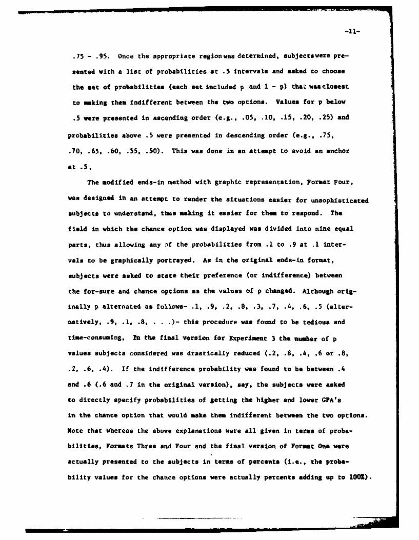
.75 -. 95. Once the appropriate region was determined, subjectswere pre-

sented with a list of probabilities at .5 Intervals and asked to choose

the set of probabilities (each set Included p and 1 - p) that was closest

to making them indifferent between the two options. Values for p below

.5 were presented in ascending order (e.g., .05,.10, .15,.20, .25) and

probabilities above .5 were presented in descending order (e.g., .75,

.70, .65, .60, .55, .50). This was done in an attempt to avoid an anchor

at.5

The modified ends-in method with graphic representation, Format Four,

was designed in an attempt to render the situations easier for unsophisticated

subjects to understand, thus making it easier for them to respond. The

field in which the chance option was displayed was divided into nine equal

parts, thus allowing any af the probabilities from .1 to .9 at .1 inter-

vals to be graphically portrayed. As in the original ends-in format,

subjects were asked to state their preference (or indifference) between

the for-sure and chance options as the values of p changed. Although orig-

inally p alternated as follows- .1, .9, .2, .8, .3, .7, .4, .6, .5 (alter-

natively, .9, .1,.8,..- this procedure was found to be tedious and

time-consuming, Zn the final vorsion for Experiment 3 the number of p

values subjects considered was drastically reduced (.2, .8, .4, .6 or .8,

.2, .6, .4). If the indifference probability was found to be between .4

and .6 (.6 and .7 in the original version), say, the subjects were asked

to directly specify probabilities of getting the higher and lower GPA's

in the chance option that would make them indifferent between the two options.

Note that whereas the above explanations were all given in terms of proba-

bilities, Formats Three and Four and the final version of Format One were

actually presented to the subjects in terms of percents (i.e., the proba-

bility values for the chance options were actually percents adding up to 1002).

~-32-

The most coherent 8ables (adjacent and distant symmetric gambles)

and formats (Formats One and Four) vere taken together to form the

three fixed state utility assessment procedures for Experiment 3. Fifteen

indifference probabilities were elicited for each subject. In the SFS

procedure a nonlinear least squares (LSQ) fit of the data points was then made

and subjects were subsequently allowed to re-assess their probabilities

using their specified set as the working set. Subjects were permitted to

re-specify their indifference probabilities a maximum of two times. It

has been our experience that after this time few significant changes are

likely to be made. If subjects did not wish to change their specified

probabilities after the LSQ fit but were also not satisfied with the

fitted probabilities, they were allowed to go directly to the questionnaire

anyway. No subject was encouraged to change his/her indifference

probabilities, only to think about the situations carefully. In this

manner as much coherence as possible among the indifference probabilities,

and thus the utilities, was obtained. Novick and Lindley (1978) have

stressed the Importance of obtainig coherence.

-13-

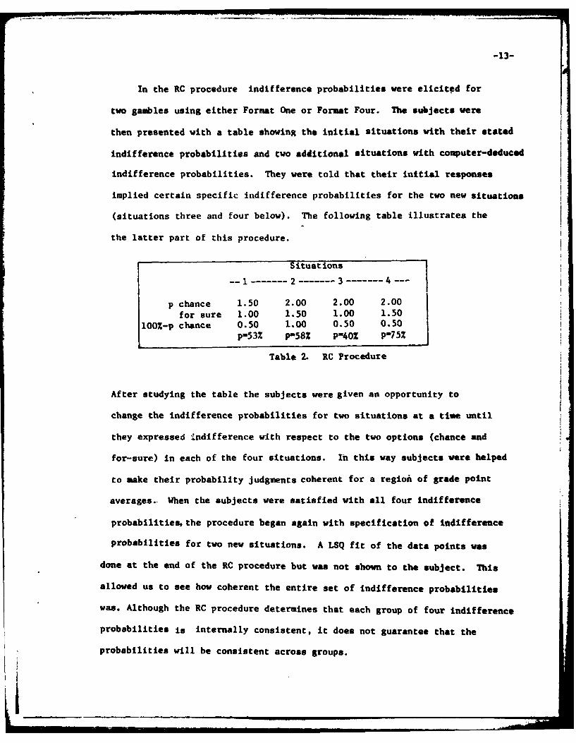
In the RC procedure indifference probabilities were elicited for

two gamb~les using either Format One or Format Four. The subjects were

then presented with a table shoving the initial situations with their stated

indifference probabilities and two additional situations with computer-deduced

indifference probabilities. They were told that their initial responses

implied certain specific indifference probabilities for the two new situations

(situations three and four below). The following table illustrates, the

the latter part of this procedure.

Situations

--1------- 2------- 3------- 4---

p chance 1.50 2.00 2.00 2.00for sure 1.00 1.50 1.00 1.50

100%-p chance 0.50 1.00 0.50 0.50p-n53% p-58% P-40% P-752

Table 2. RC Procedure

After studying the table the subjects were given an opportunity to

change the indifference probabilities for two situations at a time until

they expressed indifference with respect to the two options (chance and

for-sure) in each of the four situations. In this way subjects were helped

to make their probability judgments coherent for a region of grade point

averages.- When the subjects were satisfied with all four Indifference

probabilitiesthe procedure began again with specification of indifference

probabilities for two new situations. A LSQ fit of the data points was

done at the end of the RC procedure but was not shown to the subject. This

allowed us to see how coherent the entire set of indifference probabilities

was. Although the RC procedure determines that each group of four indifference

probabilities is internally consistent, it does not guarantee that the

probabilities will be consistent across groups.

The LC procedure presented subjects with two types of hypothetical

choice situations: (1) a for-sure and a chance option (the standard gamble

used in the SFS and RC procedures) and (2) two chance options. Again,

either Format One or Format Four was used to elicit an indifference

probability for the first situation, after which the subject was told that

that response implied that he/she should be indifferent with respect to the

two options in situation 2 for the designated probabilities. (The Option I

probabilities for Situation 2 were always 50%/50% for the two highest GPAs as

shown. Only the Option 2 probabilities for the highest and lowest CPAs changed.)

GAMBLE SITUATION 1 GAMBLE SITUATION 2

I- I I- - -- - -I - - - -IOPTION 1 OPTION 2 11OPTION 1 OPTION 2(FOR SURE) (CHANCE) 1I II

0.50 1.00 50 50% 1.00 0.0505%50 .5

- 0--- -- -- 50 0.00 25%

Table 3. LC Procedure

If the subject was not indifferent between the options In both situations,

he/she was allowed to modify the Situation 1 indifference probability.

After that probability was changed the subject was again presented with a

table similar to Table 3 above, with the Situation 2 Option 2 probabilities

now also different. This continued until the subject was indifferent with

respect to the options in each of the situations. At that point the entire

procedure was repeated with a new set of GPAs (i.e., a new gamble). As

with the RC procedure, a LSQ fit of the indifference probabilities was

computed after the subject had left.

An important feature of these experiments was that the primary

interaction was between the assessor and a preprograsmd computer

presentation of the experimental protocol. This presumably led to a

high degree of uniformity in presentation. However, research assistants did

read text and answer questions so It was possible that some inter-

assistant variability might be present.

-15- ION

Pilot Experiment 1 -Formats and gamble. for the SF8 procedure

Experiment 1 was designed to determine which of the first two for-

mats, direct probability elicitation and ends-in. for presenting gambles in

the three fixed state assessment procedures elicited the most coherent,

bias-free set of indifference probabilities. The experiment was done

in the context of the SFS procedure and the results were then extrapo-

lated to the RC and LC procedures. Experiment 1 also determined

which gambles resulted in the largest errors, in terms of log-odds

differences, and thus should be omitted from the utility assesment

procedures.

Method

Subjects. The subjects for the first part of experiment 1 were43 college undergraduates of both sexes who responded to newspaper andother advertisements. The students were randomly assigned to four groupsso that each group contained approximately the same number of subjectsof each sex. Three subjects were excluded from the analyses because theyfailed to get through the entire program and thus contributed no data tothe file. All subjects were paid $4.00 for their participation in thisexperiment.

The subjects for the second phase of this experiment were PhD levelprofessionals in the fields of Education, Psychology, Measurement, andComputer Science, and a few advanced graduate students,attending theAdvanced Seminar in Bayesian Statistics supported by the CAMA ResearchGroup at The University of Iowa. These subjects served as volunteers.

Materials and Design. For all experiments 0Omponent 31 of theComputer-Assisted Data Analysis (CADA) Monitor (Novick, et al., 1980)was modified slightly and then used in a conversational mode to presentthe formats, gambles, and incoherence resolutionmethods associated with each assessment procedure. The Monitor wasaccessed via a cathode ray tube (CRT) terminal linked to a PD? 11V03computer. Individual sessions were conducted by the research assistantswho operated the computer system, recording verbal responses given byeach participant. A complete recording of the protocol of each sessionwas stored on flexible disk and made available in herd copy through aDecwriter terminal. Data analyses were performed on the 11V03 usingdata stored on the flexible disks.

-16-

C

The following two sets of gambles were used alternately vith formatsone and two: [11--(0.0, 0.5, 1.0), (0.5, 1.0, 1.5), (0.0, 1.5. 3.0),(0.0, 1.5, 4.0), (1.5, 2.0, 2.5), (1.0, 2.0, 3.0), (0.0, 2.5, 4.0),(2.0, 3.0, 4.0), (0.0, 3.5, 4.0) and [2]--(0.0, 0.5, 4.0), (0.0, 1.0,2.0), (0.0, 1.0, 4.0), (1.0, 1.5, 2.0), (0.5, 2.0, 3.5), (2.0, 2.5, 3.0),(1.5, 2.5, 3.5), (0.0, 3.0, 4.0), (3.0, 3.5, 4.0). For the professional-level subjects, average GRE scores rather than GPAs were used. To con-struct the gamble sets, 400 was substituted for 0.0, 450 for 0.5, etc.up to 800 for 4.0. The nine gambles comprising each set were chosen soas to make the two sets of gambles as similar as possible. Even so,both formats were used with each set of gambles. The subjects in groupone responded to the first set of mixed gambles using Format One andthen the second set using Format Two. Group two subjects responded firstto set one using Format Two and second to set two using Format One.Groups three and four responded to the set two gambles first, using For-mats One and Two respectively. The design was thus a crossed formatsby gambles design with a further administration of the alternate format-gamble pair to each group. A resolution program was used to determinethe best format, in the sense of minimum mean squared deviations from aleast squares fit over all gambles made by the participant. (See dataanalysis section.) This design thus permitted examination of the for-mat effect with a check and adjustment for gamble-set and order effects.

Procedure. The experiment was conducted in a private office withsubjects being tested individually in one-hour sessions. Each subjectparticipated in one session. All instructions were standardized and printedon a CiT terminal. The research assistant read the instructions to theundergraduates to Insure that they clearly understood what was expectedof them. The professional-level subjects, however,were permitted to readthe instructions on their own, with the research assistant there toanswer any questions they may have had. Subjects were given very carefulinstructions in the meaning of indifference probabilities andIn the. eassesemt ef then. The concept of- utilitywas never mentioned, nor were a subject's utilities ever displayed becauseof the difficulty of making utility theory understandable to people withlittle or no statistical background. Some of the professional-level subjectswere familiar with Bayesian statistics and utility theory and this was dulyrecorded. Except for the exact sets of instructions printed, all of theabove was standard procedure in both of the pil6t expeirments.

In addition to the general instructions, specialized Instruc-tions were given for each elicitation format. Prior to indicating theirfirst Indifference probability, subjects were given a chance to reviewthe instructions to insure that they clearly understood what they wereto do. After the introductory paragraph and before the instructionsconcerning the nature of the choice situations, the following four ques-tions were asked of undergraduates to get them to begin considering howtheir final grade point average would affect their future opportunities:

-17-

1. WHAr YEAR IN SCHUUL AkU& YOU?

2. WHAT IS YOUR MAJORS'

3. UPON COMPLETION OF YUL)Uk ACHELOk'S [EGREE, WHICH OF THE FOLLOWINGIPlSSIBI..LIIES DO Y01 C0WNiIII'I H MOSI LIKELY IO OCCUR?

GiUA|'I.JAL 5 I'I.H IY ii) IkF.: I . L' L Ii: (iRI.E I IVI L.UtNALIUArE STIlJLY It) V1' L-VLL OR F'OFESSIONAL SCHOOLEMPLOYMENT-

4. II WHAT1 LXI'ENI 110 YiU FELL. YOUR CUMULATIVE GPA WILL AFFECT WHAT YOU WANT TOIJI IN HIL FIJI RIF?

k 1R: -'1 I.. Y

AIht H 1A 1VERY L.IILEANSW LR'!

In order to get the professional-level subjects to begin thinkingabout the Importance of GRE scores In selecting first-year graduatestudents, the following four questions vere asked of them:

I- WHAT IS THE ACADEMIC DISCIPLINE FOR WHICH YOU MIGHT SERVE AS CHAIR OFGRADUATE ADMISSIONS?

2. WHAT IS THE APPROXIMATE MEAN AVERAGE GRE SCORE OF FIRST-YEAR GRADUATESTUDENTS IN THE DEPARTMENT IN WHICH YOU MIGHT SERVE? RECALL THAT EACHSUBTEST OF THE GRE IS ON THE SCALE 200-900 WITH A NATIONAL MEAN OF ABOUT500 AND STANDARD DEVIATION OF ABOUT 100.ANSWER?

3. DO YOU FEEL THAT THIS SCORE IS A GOOD PREDICTOR OF FUTURE PERFORMANCEIN YOUR PROGRAM?

1, YESP VERY GOOD PREDICTOR2. YES, MODERATELY GOOD PREDICTOR3. AVERAGE PREDICTOR4# NOP FAIR PREDICTOR5. NOv POOR PREDICTOR

ANSWER?

4. DO YOU FEEL THAT THE TEST SCORE IS AN IMPORTANT PIECE OF INFORMATION INSELECTING STUDENTS?

1. YES, VERY IMPORTANT2. YES, IMPORTANT3. NO STRONG FEELINGS EITHER WAY4. NO, NOT VERY IMPORTANT5. NOP NOT IMPORTANT AT ALL

ANSWER?

-318-

A complete set of the instructions given to these subjects may be foundin Appendix B. Except for a few slight modifications to make the instruc-tions easier to understand, the saw instructions were used for the pro-fessLonal-level subjects as for the undergraduates. Thus to derive theInstructions for the undergraduates, one can simply substitute "finalgrade point average at graduation" for "admittance of a student with aparticular average GEE score." The paragraphs introducing the ecenariowere different for both sets of subjects and thus both introductionsare reprinted in Appendix 3.

After providing indifference probabilities for both sets of gambles.subjects were shown a least squares fit of the date points. They weretold that the computer had generated a set of indifference probabilitiessimilar to theirs in order to help them specify a coherent set of pvalues. If subjects were not satisfied with the fitted probabilities,they were given an opportunity to change any or all of their specifiedprobabilities. A new least squares fit based on the revised probabili-ties was then computed. Subjects were allowed to revise their indiffer-ence probabilities twice if they so desired and thus were able to seeup to three different sets of fitted probabilities. Any subject who hadnot accepted the fitted probabilities by the third time was asked to doso then because it has been our experience that by then neither set ofprobabilities is likely to change substantially. When the subject ac-cepted the fitted probabilities the formal part of the experiment wascomplete.

At the end of the experiment all subjects responded to a questionnairecalling for an evaluation of the experiment as a whole. If subjectsinquijed further about the purpose of the experiment they were told thatthe results would be used to help design procedures for making it easyfor persons to decide on desirable gambles.

-19-

Pilot Experiment 2 - Formats for standard f ixed state gambles

Experiment 2 was an extension of experiment 1; it's purpose was to

determine which of two new formats (formats 3 and 4) for eliciting

indifference probabilities provided the most coherent, bias-free set of

probabilities. A revised set of gambles was used.

Method

Subjects. The 10 subjects were graduate students enrolled in theBayesian Statistics I class at The University of Iowa. They served asvolunteers.

Design. The design was a crossed formats by gambles design with afurther administration of the alternate format-gamble pair to each groupas In experiment 1. Gamble set one consisted of the following adjacentgambles: (0.5, 1.0, 1.5), (1.0, 1.5, 2.0), (1.5, 2.0, 2.5), (2.0, 2.5,3.0), and (2.5, 3.0, 3.5). Gamble set two included the following distantsymetric (specifically, two-apart) gambles: (0.0, 1,0, 2.0), (0.5.1.5, 2.5), (1.0, 2.0, 3.0), (1.5, 2.5, 3.5), and (2.0, 3.0, 4.0). Inaddition, whichever set of gambles was responded to first, regardlessof format, also included (0.0, 0.5, 1.0) and (3.0, 3.5, 4.0) so thatthe first seven situations were sufficient to determine a utilityfunction. The second set of gambles to which a subject responded inclu-ded (0.0, 2.0, 4.0) and (1.0, 2.5, 4.0). Thus each subject indicatedindifference probabilities for a total of 14. situations. Computationof format errors did not consider the above four gambles. These 14 gambleswere chosen on the basis of the results of Pilot Experiment 1. Theutility gambles were excluded because subjects found them difficultand because they generally resulted in large log-odds differences betweenthe assessed and fitted indifference probabilities. The four experi-mental groups were constructed as in the previous experiment.

Procedure. The procedure was the same as in experiment 1 exceptthat each subject indicated only 14 indifference probabilities ratherthan 18.

-20-

Zxperiment 3 - Comparison of SIPS, RC, and LC procedures

The purpose of this experimeat was twofold. First we were interested In

whether the original format (Format 0ne) or a new format (Format Four)

resulted in the most reliable (coherent) and bias-free set of utilities

(indifference probabilities). The major conclusion of Interest, however,

was which of the three utility assessment procedures provided the best

set of utilities.

Method

Subjects. Although 50 subjects were run, 10 had to be excluded from

the data analyses because a) they failed to get through the entire

procedure or b) their indifference probabilities were too incoherent for

a least squares fit to be computed. The remaining 40 were randomly assigned

to three groups, with approximately the same number of subjects in each

group. Subjects were paid $4.00 upon completion of the experimental

session. Students who had participated In either of the previous pilot

experiments were not allowed to be In this experiment.

Design. In this experiment format was a within-subject variable

while assessment procedure and format order were between-subject variables.

Each group of subjects used only one of the three procedures. Half of

the subjects in each group used Format One followed by Format Four, while

the other subjects used Format Four first. There were three or four

subjects of each sex in each format-order group for each procedure.

Format One, direct elicitation, was chosen because It is the format

most often used with utility assessment procedures. Format Four, on the

other hand, was chosen because Pilot Experiments 1 and 2 suggested that

It may be better than Format one, in the sense of being easier for

assessors to use, in inducing more coherent responses from them, and in

-21-

seemingly being less influenced by the anchoring effect. The gambles were

chosen on the basis of the sane informktion as led to the format choices mad,

in general, were the ones subjects found easiest to chink about. The only

utility gamble used is (0.0, 2.0, 4.0) because subjects generally found

it very difficult to specify indifference probabilities for utility gambles.

As a group, the utility gambles led to much more incoherent judgments

than either the adjacent or distant symmetric gambles. There were a

few other gambles (e.g. (0.0, 0.5, 1.0) and (3.0, 3.5, 4.0))which were

a little difficult for subjects but these were retained because they

were needed to compute the utility function. Also, these gambles were not

as bad as the utility gambles.

Two mixed sets of gambles (containing both adjacent and distant

symmetric gambles) were constructed. The seven gambles in Set One were

sufficient to compute a utility function and were used as the basis for

determining the fitted probabilities for the SFS procedure. Set Two

included all of the remaining adjacent and distant gambles. The gamble

sets were:

SET ONE - (0.0, 0.5, 1.0), (0.0, 1.0, 2.0), (0.5, 1.5, 2.5), (1.5, 2.0,

2.5), (1.0, 2.5, 4.0), (2.5, 3.0, 3.5), and (3.0, 3.5, 4.0).

SET TWO - (0.5, 1.0, 1.5), (1.0, 1.5, 2.0), (0.0, 1.5, 3.0), (1.0, 2.0,

3.0), (0.0, 2.0, 4.0), (2.0, 2.5, 3.0), (1.5, 2.5, 3.5), and (2.0, 3.0, 4.0).

These two sets were used as presented above for both the SFS and LC

procedures. Because of the manner in which situations three and four were

generated in the RC procedure, it was necessary to substitute (0.0, 1.0, 2.0)

and (2.5, 3.0, 3.5) for (0.0, 1.5, 3.0) and (2.0, 2.5, 3.0) in Set Two

for that procedure. Thus subjects responded to these two gambles twice

in the RC procedure but only once in the other two procedures.

-22-

Subjects always responded to the Set One gambles before proceeding

to the Set Two gambles. The forusm, however, as explained above, were

counterbalanced with half of the subjects using each procedure receiving

Format One-Set One/Format Four-Set Two and the other half receiving Format

Four-Set One/Format One-Set Two. This was done in order to enable us

to look at format effects within and across procedures.

The design was thus a crossed procedure by sex by formt-order design.

Gamble set order, however, remained fixed.

Procedure. The procedure for this experiment was in general the same

as that for the two pilot experiments. There were, however, a few

differences. First, the exact procedure followed by each subject was

obviously dependent on whether he/she used the SFS, RC, or LC procedure.

In the previous studies all subjects used the SFS procedure. Also, in

this experiment we had subjects write down their utility function for

grade point averages (from 0.0 to 4.0) on a scale of 0-100 after they

had completed the probability elicitation procedure. This question was

in addition to the general written questionnaire.

-23-

Data Analysis. Ideally a data analysis would compare ansessed utilities with

true utilities. Unfortunately there is no assured method of measuring

true utilities. However, an approach commonly adopted in psychological

testing seems relevant. Assuming that assessed utilities involving

extensive measurements with averaging and/or adjustment are likely to

be close to true utilities, the reliability or accuracy of Individual

component procedures can be assessed by comparing utilities from these

procedures with those from the more extensive measurement. The testing

analogy would be to evaluate each of several short measures of a

construct by relating each measure to the average overall measures or

perhaps to some factor analytically defined composite.

A variety of methods of comparing measures is possible. We have

chosen to use an approach that is closely related to the least squares

fitting procedure (Novick & Lindley, 1979). Consider, for example,

the comparison of two methods (I and II), each Involving a fixed

state assessments for N points, with coherence adjustment. Denote the

N utilities obtained for the two methods of U Il, .... U IN and U 112 ,

... ,P U .IN Denote the N assessed utilities after the least squares fit

and resolution involving the 2. gambles by Ulf .... U N. The symbols

* U1 ui:~and V will be used to denote vectors containing these ordered

utilities. For each gamble used there will be a probability Implied

by each of the vectors VI, VII, and V. We denote these as value

T III .. in, 'Im' l ...,' V Ila' and w., ...,w and the corresponding

vectors by w~ i~and w. Then taking the log odds (y - log((l)I

-24-

of the individual probabilities we can evaluate each method by

considering discrepancies between transformed probabilities for

the Individual methods and the corresponding values for the final

fitted utilities. In these analyses we shall take the values yl'

"". YN for the resolved log-odds probabilities as "true" values

and consider values y,,, ", VN and yI 1 ... I',¥IN as measure-

ments containing independent, normal, homoscedastic errors. The symbols

!. I and 1,, will denote the vectors of log-odds values. Data

analysis will then involve the comparison of the average bias and

average squared error for the methods in question. Symbolically the

comparisons are (y 11-YI) (Y1 2 -Y 2 ), ... (YIN-YN) and (ylll),

(Y112-Y2)# ...,I (YI9-YN). In the several experiments this involves

comparing various categories of method, format, type of gamble, and

individual gambles.

The normality and homoscedasticity assumptions are reasonable

on theoretical grounds by virture of the log-odds transformation and

are supported by data exploration. Slightly less comforting is the

assumption that errors are independent (Novick & Lindley, 1979).

However, measurement independence is a standard casual assumption that

seems to be as acceptable here as in other applications. Failure of

this assumption would be Important primarily if it were differential

between methods being compared.

-25-

Results

Two dependent variables, Mean Absolute Error (MAE) and Greatest

Absolute Difference in Utilities (GADU) were considered as criteria

of subjects' performance. These measures and the relationship between

them will be discussed in detail below. The tables presenting the

results to be discussed are located in Appendix D.

Analysis with MAE as the Dependent Variable

The primary criterion of a subject's performance was Mean Absolute

Error, an index of overall consistency. Three types of MAE measures

were utilized in the analysis. The overall measure for each subject

was obtained by averaging the 15 absolute log-odds differences between

his/her specified probabilities and the probabilities obtained from the

least-squares fit (see Table 4). The distribution of MAE was determined

to be approximately normal by CADA's Normal Probability Plot. The

grand mean and the standard deviation for the measure were .4065 and

.1800, respectively, with observations ranging from .0555 (very consistent)

to .8540 (very inconsistent).

Because of the interest in performance under each of the two formats,

two additional MAEs were computed for each subject: one for performance

using Format I and one for performance using Format 4. The cell means

and a-counts for the analysis of the effects of Procedure, Format,

and Sex are presented in Table 5.

A final measure of MAE was considered appropriate for some aspects of

the analysis. This variable may be described as the difference between

the MAE obtained under Format I and the MAE obtained under Format 4

(A MAE -4). It was hypothesized that MAE would be somewhat greater than

MAE 4, and so a small positive value was expected for each individual.

-26-

As can be seen from Table 6, the grand mean for AMAE1 -4 was slightly

positive (H - .0046), although there were many exceptions for the

individual observations and also for several of the cell means.

A two-way ANOVA was applied to the new variable AMAZB1-4 in order

to determine the extent to which it was affected by Procedure and Sex.

Table 6 shows the marked Procedure effect upon AHABE4 (392 of the total

variance in &MAEI_4 can be accounted for by Procedure). In particular,

the average AMAE_ 4 for the RC procedure was relatively high (.0587),

indicating a high degree of interaction between this procedure and the

formats. The LC and SFS procedures evidenced lesser interactions with the

formats (average AMAE1-4 for SFS - -.0242, and average AMAE 1-4 for

LC - -.0185). These results are discussed in more detail below.

Main Effects for MAE

Procedure

While it was difficult to have prior convictions about the

magnitude of the Procedure effectsthe authors did have preconceptions

about the efficacy of the three assessment procedures. In particular,

it was expected that the Regional Coherence Procedure would be most

successful in eliciting consistent responses, that the Standard Fixed

State Procedure would be least effective, and that the Local Coherence

Procedure would be intermediate. However, as seen in Table4,

these expectations were only partly realized. The MAE for RC, SFS,

and LC were .3923, .4021,and .4295, respectively. The poor

performance with the LC procedure was thought to be due to the lack

of sophistication of the undergraduate subjects and might not be

replicated with a sample of subjects who had had more statistical

training. A prnedure for making the LC prosedure sore useful might

-27-

consist of 1) revising the presentation to make it more comprehensible

to neophytes, 2) rewriting instructions to make its use more attractive,

or 3) using it with only more sophisiticated subjects.

Format

The effect of Format on MAE was surprisingly small (see Table 5).

We had expected that Format 4 would yield more consistent results. Format

may be considered a within subject factor Since each subject was run

under botn formats, and so 40 observations were obtained for each of

of the two formats. The average MAE under Format 4 was .4040, which

could not be considered to be appreciably different from the MAE of .4103

obtained under Format 1. The Format factor might, however, be considered

interesting due to its interaction with Procedure (to be discussed below).

Sex of Sublect,

The subjects' sex was found to have a strong effect

on performance as measured by MAE. The greater consistency on

the part of the female subjects was interesting for

several reasons. First of all, it was expected that males would

have a more extensive background in quantitative disciplines and

might therefore excel in tasks requiring complex reasoning abilities.

Secondly, there was a problem with students who had made appointt

for the experiment failing to report, and this "no-show" tendency

was markedly more prevalent in male subjects. Therefore, it was

expected that the males who did keep their appointments would be

-28-

more highly motivated and more likely to perform weil. While neither

of thee hypotheses was borne out by the HAS data, alternative

explanations for the greater female consistency might be offered.

In particular, the results could be seen as consistent with the

general finding that women are more careful than men on many tasks.

They might, therefore, be expected to perform better In an experiment

which requires great deliveration and painstaking accuracy.

Interaction Effects

Procedure by Format Interaction

As discussed above, Procedure had a strong effect on the variable

6MA1- 4 ' accounting for 39% of its variance. A complex interaction

between Format and Procedure was particularly apparent under the

RC procedure (see Table 5). '

Since one of the objectives of the experiment was to determine

which combination of Procedure and Format would yield the most

consistent results, particular attention should be paid to the

average HAEs presented in Table 5. It should be noted that the

RC procedure used in conjunction with Format 4 yielded the lowest

average MAE (.3615). This finding

confirmed expectations of both the relative efficacy of the RC

procedure and the relative ease of Format 4. It might also be

noted that this winning combination was particularly effective for

the 6 female subjects who achieved very consistent results G-.2846)through its use. On the other hand, the LC procedure coupled with

-29-

Format 4 produced the least desirable results (x m.4387), although

these results did not differ greatly from those obtained under the

LC procedure in conjunction with format 1 (xu.4202).

Procedure by Sex Interaction

Table 4 demonstrates that "iea performed best under the LC

procedure while female performance was worst under this procedure.

The females apparently profited from the RC and SFS procedures

(achieved means of .2978 and .3285. respectively) while the mlss

did rather poorly under these two procedures (with mean performance

of .4803 and .5046, respectively).

Format by Sex Interaction

Table 5 indicates little interaction between Format and Sex.

Males performed only somewhat better under Format 4 than under

Format 1 while there was essentially no difference in female

performance as a function of format.

Analysis with GADU as the Dependent Variable

A second criterion of performance was the Greatest Absolute

Difference in Utilities (GADU) which may be described as an index of

congruence between the subject's stated utility function (written on

a piece of paper before or after the experiment) and the utility

function obtained by his specification of probabilities during the

procedure. It was believed that this might be a better Indicator of

how veil the subject was able to use the procedure to reproduce his

CPA gambling behavior than would the consistency index (KA5)

described above. This assumption was based on the observation of

cases in which subjects appeared to quite consistent (perhaps merely

by specifying .5 or some other value for mest of the situations), but

had fitted utility functions which deviated greatly from their

-30-

stated functions.

The hypothesis that consistency has little or no relationship

to success in reproducing utility functions was confirmed by obtaining

a Spearman Rank-Order Correlation coefficient for the ranks of each

of 40 observations on overall MAE and GADU. The rof -.0858 points to the

fact that there is essentially no correlation between these two skills

and also helps to explain the reversals in results when observations

for these two variables were broken down by Procedure, Sexand

Format (see analysis for MAE above and GADU below). This

lack of correlation may cast doubt on one or both of the indices as

measures of successful completion of the gambling task or it may be

a function of the rather small undergraduate sample tested. On

the other hand, the essentially zero correlation may indicate that

both indices are valid measures of performance but that they identify

very different skills.

For the purposes of this analysis, the 40 subjects were divided

into two groups depending on the format they used first in the utility

assessment procedure. This was done for the following reason: The

15 gambles used in this experiment were divided into two sets. Set 1.

containing 7 gambles, was always responded to first while Set 2,

consisting of 8 gambles, was always responded to second. Since the

for-sure options in the first gambles contained all of the CPAs between

0.5 and 3.5 (at 0.5 intervals), a utility function could be computed

from the Indifference probabilities for Set 1. However, this was

not possible for the Set 2 gambles. Thus, for some of the subjects

the fitted utility function was based on performance under Format I

-31-

while for the remainder of the subjects the function was based on

performance under Format 4. Consequently, there appear to be half

as many subjects per format in Table 7 than in Table 5.

The 40 observations on GALU are presented in Table 7 along vith

the twelve cell means when GADU was broken down by Procedure, Format,

and Sex. Table 8 provides summary data. The observations on GADU

were essentially normally distributed with a mean of .3384 and a

standard deviation of .18. They ranged from .1153 (very close

approximation of stated utility function) to .8104 (very poor

approximation).

Main Effects for GADU

Procedure

The Procedure effect is particularly interesting because of the

ordering of the effectiveness of the procedures in eliciting a small

GADU. As Table 7 indicates, the RC procedure produced the smallest

GADU. The LC and SFS procedures were clearly less effective in

obtaining utilities which were similar to the students' stated utility

functions. It might be claimed that the checking devices offered by

the two coherence procedures were helpful to subjects in the sense

of making the probabilities upon which their utilities were based

conform to the GPA utilities they had in mind. It should also be noted

that the IC procedure led to better results on both the MAN and the

GADU criteria which, s mentioned above, are hypothesized to measure

two distinct skills.

Format

The Format effect was once again very small, as demonstrated by

Tables 7and B. Since utilities were computed only from the first

-32-

seven gmbles, only one measure of GAN vas obtained for each subject,

thereby permitting the three-factor analyuid suirized in the two

tables. The mean GADU for the subjects in the Format 4 group was only

slightly lower than that for the subjects In the Formt I group

(xp4".3448 vs. 11- .3597).

Sex of Subject

The subject's sex once again had an important effect on the

criterion variable. Perhaps, the most Interesting observation that

may be made here is that sales (with a mean GAN of .3152) were

clearly superior to females (with a mean GADU of .3836) in minimizing

the difference between their stated and fitted utility functions

(See Table 7). This contrasts with the superior female performance

on obtaining consistent results as revealed by the MAR index.

Interaction affects

Procedure by Format Interaction

The complexity of this interaction for dependent variable GADU

was somewhat greater than for AB (sea Table SA). For the RC Procedure,

performance did not differ as a function of format. The IX procedure

seemed better in conjunction with Format I than Format 4, while the

reverse was true for the SFS procedure.

Procedure by Sex Interaction

A small interaction was noted between Procedure and Sex, as

Indicated in Table 8C. The results show that performace under the LC

procedure evidenced the greatest variation as a function of sex. The

GAN results differ from the HAS results in that GM shove RC to be

best for both mles and females wbile MAK indicates that femiales

-33-

perform best under RC and sales perform beat under LC.

Sax by Format Interaction

This Interaction was very slight. Females performed only somewhat

better under Format 4 than under Format 1 while there was essentially

no difference in male performance as a function of format. GOLDU and

MAE were consistent in showing that performance under each format did

not differ as a function of the sex of the subject.

Procedure by Format by Sex Interaction

The three-way interaction was large and striking as illustrated

in Figure 1. The effect of format varied as a function of sex and

utility assessment procedure.

Effect of Statistical Training on Performance

It was hypothesized that students who had had some statistical

training would perform better than those who had had none. Indeed,

the 14 students who had had one or more hours of statistics obtained

an average MAE of .3411 while those with zero hews of statistics obtained

an average MAE of .4012. When GADU was the criterion, the students with

statistical training obtained an average score of'. 3061 while those with no

training obtained an average score of .3583.

General Discussion

Several conclusions may be drawn from the three experiments

conducted. First, adjacent and distant symetric gambles appear to

be more useful than utility gambles. Second, the Regional Coherence

procedure was found to lead to superior results on both the MAE and

GADU criteria. Finally, neither Format provided utilities move cofgruent

-3'-

with initially stated utilities than the other. No conclusion could

be drawn as to whether the fault lay in the initially stated or

experimentally elicited utilities.

When taken together, however, the Regional Coherence procedure

and the modified ends-in format (Format 4) seen promising, at least

for people with moderate to no statistical training. Unfortunately,

while the undergraduates participating in this experiment came from

a wide range of academic disciplines, they may have lacked either

the ability or motivation to fully appreciate and understand the

complexity and importance of the gambling situations. A more

statistically inclined sample of people in another environment might

well get the best results wi-Sh a different combination of procedure

and format.

While even the trained statistician could no doubt benefit from

the use of a utility assessment procedure with coherence-checking

capabilities, the "naive" person would seem to gain the most from

use of such a procedure in the Interactive environment of CAM. And

for these persons Experiment 3 suggests that Regional Coherence with

a graphic ends-in method of eliciting Indifference probabilities,

if not the ultimate answer, is at least somewhat more profitable than

its rivals. We feel confident that this combination or some derivative,

whien used to assess utilities in a real-life situation, will prove

useful.

Appendix A -35-

Evolution of the Formats

Format I - Direct Elicitation

I. As originally on CAA:

FOR GAMBLES P THAT KAKES

SURE P I-P YOU INDIFFERENT

0.50 1.00 0.00 ? .5

1.00 1.50 0.50 ? -

2. As for Pilot Experiment IA:

CPA CPA I

I P 1.0

I FOR SURE 0.5 GABLEI

I 1-? 0.0S------------- IWhat value of P makes you indiffereat between thefor-sure and the chance options?

3. As for Pilot Experiment IS:

Format One

I CPA I I GPA II 1 1 3.5 PII FOR SURE 2.51 1 CHA1iCE II I 1.5 I-P I

What value of p makes you inaifferent between the for-sureand the chance options?

4. As for Experiment 3:

Format One

FOR SURE OPTION CLAIUCE OPTION

I GPA I C CPA II I I 3.5 pz II 2.5 I I II I 1 1.5 ,OO-P I

What value of p makes you indifferent between the for-sureand the chance options?

-36-

Fornt 2- Ends-In

1. As originally on CADA:

OPTION:

I P 1.00 11 0 INDIFFER

I F0o SURE 0. 50 GAMBLE I I FO SURE1 2 CHANCE

I 1-P 0.00 I 3 RESTART

Which would you prefer if p a .XX ?

2. As for Pilot Experiment lA:

Format Two

S--------------------OPTION

I GPA I I CPA 1 0 INDIFFERENTI I I 3.5 P I 1 FOR SUREI FOR SURE 2.5 I I CHANCE I 2 CHANCEI I 1 1.5 I-P 1 3 RESTART---------------------------------------------------

Which option would you prefer if p - .XX?

Format 1 - Quartering

1. Original Conception:

I CPA I I GPA I OPTIONI I I 3.5 75Z I 1 FOR SUREI FOR SURE 2.5 1 I CHANCE I 2 CHANCEI I 1 1.5 25% 1 3 RESTART

Which option do you prefer?

I PA I I CPA II I I 3.5 P II FOR SURE 2.5 I I CHANCE II 1 1 1.5 Q I

Choose the set of P and Q values that will dke you indifferentbetween the for-sure and the chance options.

P 75% 70Z 65% 60% 55% 501Q 25% 30Z 352 402 452 501The P value that makes you indifferent is?

-37-

2. As for Pilot Experiment 2:

Format Three

yOR SURE OPTION A CiwNCs OmON

I CPA I I CPA CNANCE I OPTIONI I I 3.5 752 I I FOR SUREI 2.5. POR SUREI I I 2 CNAXCEI I I 1.5 252 I 3 RESTART

Which option do you prefer?

_.FOR SURE OPTION CHANCE OPTION -

I CPA I I CPA CRANCE II I I 3.5 P I1 2.5 FOR SURE I I II I I 1.5 Q I

Choose the set of P and Q values that will make you indifferentbetween the for-sure and the chance options.

P 75Z 70Z 652 60Z 52 50Q 25Z 30% 35% 402 452 502

The P value that makes you indifferent is ?

Format 4 - Modified Ends-In

1. Original Conception:Format Four

1002 A 202 602 OPIN0 IND'LlqqJNT

I GPA I IGPA I CPA I 0 U RE1 FOR SUREI I I I I 2CHANCE1 2.5 1 11.5 1 3.5 I~ 3 RESTARTI I I II

FOR SURE CHANCE

Which option do you prefer?

-38-

B

1002 1002-P

M OA I IGCA CPAI I I

I 2.5 1 11.5 3.5I II

Fo suu. o r -o ----- CMIE OPTIYour Indifference probability, P, has been determined to be

betveen 40% and 602.

Value of P?

-39-

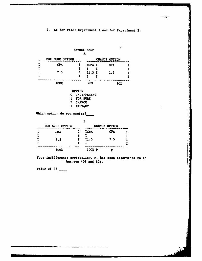
2. An for Pilot Experiment 2 and for Experiment 3:

Format FourA

FOR SURE OPTION CHANCE OPTION

I CPA I IGPA I GPA II I I I I2 2.5 1 11.5 1 3.5 I

I I I I I

-------------- I---------------------100 20% 80%

OPTION0 INDIFFERENT1 FOR SURE2 CHANCE

3 RESTART

Which option do you prefer?

B

FOR SURE OPTION CIWICE OPTION~~~~ ------------ - - -

I G(A I IGPA CPA II I I II 2.5 I 11.5 3.5 1I I I I

1002 1002-P P

Your indifference probability, P, has been determined to bebetween 402 and 602.

Value of P?

-40-Appendix B - Instructions

PILOT KIJUIHDU 1

A. Introduction:

experiment 1AUHE PURPOSE OF THIS EXPERIMENT IS TO STUDY GAMBLING BEHAVIOR WHEN *iHE OBJECTOF: THE GAMBLE IS AN IMPORTANT FICTOR RELATING TO A COLLEGE STUDiENT'S FUTUREOPPORTUNITIES, NAMELY, CUMULATIVE GRADE POINT AVERAGE (GPA) AT GRADUATION.

YOU WILL BE PRESENTEDI WITH SEVERAL. SITUATIONS INVOLVING CHOICES BETWEEN GAMBLES,AND SURE' THINGS. YOU ARE TO IMAiINE lHAf /FITH OUTUME (IF IHE OPTIION YOU CHOOSEWILL. RESULT IN THE FIXING OF A f rF'll LILAN (WI-F:A O'IN YOUR FERMANE" T UNI IVf;:.SITYi'FCORD.,

WHILL WE REALIZE THAT YOU ARE NOI ACCUSTOMEI TO GAMBLING ON YOUR (RAItE POINTAVERAGE, WE WOULD L.IKL YOU TO rRY I0 RESPOND AS YOU WOULD I[ IHESE WERE ACTUALSITUATIONS, CONSIDER C[AREFL.L.Y WHAI EACH I3RAIE POilI* AVERASfEI WfAU.D " MEAN TO YOU..r GRAI)UAI 1ON ANI HOW EACH W(IUI.. I' A1fU CTI YOUR GOALA; FOI-: FURTHER' E DUGI.AT ION ANDFUTURE EMPLOYMENT.

iHESE GAMVLES CANNOT, OF COURSE, FIE CARRIEI OUT IN REAL LIFE; HOWEVERP THE•.TUATION SHOULD BE MEANINGFUL TO YOU. THE PURPOSE OF THE EXPERIMENT IS TOISTUDY GAMBLING BEHAVIOR WHEN THE OUTCOMES HAVE SUBSTANTIAL IMPORTANCE RELAT-iN;NG TOL A STUDENT 'S FUTURE.

experiment 11

THE PURPOSE OF THIS EXPERIMENT IS TO STUDY GAMBLING BEHAVIOR WHEN THE OBJECTOF THE GAMBLE IS AN IMPORTANT FACTOR RELATING TO THE QUALITY OF THE GRADUATESTUDENTS IN A PHD PROGRAM, NAMELY, THE AVERAGE OF THEIR VERBAL AND GUANTI-TATIVE GRADUATE RECORD EXAMINATION (GRE) SCORES. YOU ARE TO THINK OF YOUR-SELF AS THE CHAIR OF THE ADMISSIONS COMMITTEE OF THE GRADUATE DEPARTMENT WITHWHICH YOU CAN MOST COMFORTABLY IDENTIFY.

AS CHAIR OF THE COMMITTEE, YOUR OPINIONS ARE HIGHLY REGARDED AND THE STUDENTSYOU RECOMMEND ARE LIKELY TO BE SENT ACCEPTANCE LETTERS. YOU, OF COURSE,WOULD LIKE TO ADMIT THE STUDENTS WITH THE HIGHEST AVERAGE GRE SCORES, GIVENTHAT ALL OTHER RATING FACTORS ARE EQUAL.

FOR THE PURPOSES OF THIS EXPERIMENT, HOWEVER, A MORE DIFFICULT TASK WILL BEPRESENTED TO YOU. YOU CANNOT SIMPLY RECOMMEND THE STUDENTS WITH THE TOPTEST SCORES. RATHER, YOU WILL BE PRESENTED WITH SEVERAL SITUATIONS INVOLVINGCHOICES BETWEEN GETTING A STUDENT WITH A PARTICULAR AVERAGE ORE SCORE FORSURE, AND A GAMBLE WHICH WILL GET YOU A STUDENT WITH A HIGHER SCORE IF YOU WINOR ONE WITH A LOWER SCORE IF YOU LOSE.

-41-

WHILE WE REALIZE THAT YOU ARE NOT ACCUSTOMED TO GAMBLING ON THE GRE SCORESOF THE STUDENTS TO BE ADMITTED TO YOUR GRADUATE PROGRAMP WE WOULD LIKE YOU TORESPOND AS YOU WOULD IF THESE WERE ACTUAL DECISION SITUATIONS. CONSIDERCAREFULLY WHAT IT WOULD MEAN TO YOU? YOUR UNIVERSITY, AND ALL OTHERS CONCERNED"TO ADMIT A GRADUATE STUDENT WITH A PARTICULAR AVERAGE GRE SCORE.

THE SITUATIONS THAT WILL BE PRESENTED TO YOU CANNOT, OF COURSE9 BE CARRIEDOUT IN REAL LIFE; HOWEVER, YOUR RESPONSES TO THESE IDEALIZED SITUATIONS MILLTELL US SOMETHING ABOUT YOUR BEHAVIOR IN MORE REALISTIC SITUATIONS. THEPURPOSE OF THE EXPERIMENT IS TO STUDY GAMBLING BEHAVIOR WHEN THE OUTCOMES HAVESUBSTANTIAL IMPORTANCE RELATING TO THE NORMAL FUNCTIONING OF A GRADUATEINSTITUTION.

B. General Instructions - Both Formats

IN THIS EXPERIMENT YOU WILL BE PRESENTED WITH SEVERAL HYPOTHETICAL CHOICE SITU-ATIONS CONSISTING OF 4 FOR-SURE AND A CHANCE OPTION, THE FOR-SURE OPTIONOFFERS YOU THE CERTAINTY OF KNOWING THE OUTCOME IF YOU CHOOSE THAT OPTION.THE CHANCE OPTION OFFERS YOU A PROBABILISTIC CHANCE AT TWO POSSIBLE OUTCOMES.

FOR EXAMPLE, THE FOR-SURE OPTION COULD HAVE YOU ADMIT A STUDENT WITH ANAVERAGE GRE SCORE OF 550. THE CHANCE OPTION COULD THEN OFFER YOU THE CHANCEOF ADMITTING SOMEONE WITH A SCORE OF 750 WITH PROBABILITY P (WHERE P CAN BEANY VALUE BETWEEN ZERO AND ONE) OR A PERSON WITH A SCORE OF 500 WITH PROBA-BILITY 1-P.

ASSUMING THAT YOU PREFER TO ADMIT A STUDENT WITH A SCORE OF 750 TO ONE WITH ASCORE OF 550 TO ONE WITH A SCORE OF 500 AND ASSUMING THAT YOU ARE GIVEN ACHOICE BETWEEN THE FOR-SURE AND CHANCE OPTIONS, YOUR DECISION AS TO WHICHOPTION YOU WOULD PREFER TO TAKE WILL DEPEND UPON THE VALUE OF P, THE PROBA-BILITY OF ADMITTING A STUDENT WITH AN AVERAGE ORE SCORE OF 750 UNDER THECHANCE OPTION.

THIS PARTICULAR CHOICE OF ADMITTING A STUDENT WITH A SCORE OF 550 FOR SURE

VERSUS THE CHANCE OF ADMITTING STUDENTS WITH SCORES OF 750 AND 500 WITH

PROBABILITIES P AND I-P, RESPECTIVELYP WOULD BE DISPLAYED ON THE SCREEN

AS FOLLOWS.

---------------------------- ---------------------------

I ORE I I ORE II I I 750 P I

I FOFR SURE 550 I I CHANCE II I I 500 1-P II I I I

-42-

FOR P VALUES CLOSE TO ONE YOU WILL PREFER THE CHANCE OPTION BECAUSE IT WILLPROBABLY RESULT IN THE ADMITTANCE OF A STUDENT WITH AN AVERAGE ORE SCORE OF

750 RATHER THAN THE ADMITTANCE OF ONE WITH A SCORE OF 500. THE FOR-SUREOPTION, ON THE OTHER HAND, SAYS THAT THE ADMITTED STUDENT WILL ONLY HAVE ASCORE OF 550.

FOR VALUES NEAR ZERO, HOWEVER, YOU WILL PREFER THE SURE THING (ADMITTINGA STUDENT WITH A SCORE OF 550) BECAUSE THE CHANCE OPTION WILL PROBABLY RESULT

IN THE ADMITTANCE OF A STUDENT WITH A ORE SCORE OF 500. THIS IS BECAUSE A PVALUE NEAR ZERO MEANS THAT THE VALUE OF 1-P, THE PROBABILITY OF ADMITTINGSOMEONE WITH AN AVERAGE GRE SCORE OF 500, WILL BE NEAR ONE.

FOR SOME UNIQUE INTERMEDIATE VALUE OF P YOU SHOULD BE INDIFFERENT BETWEENTHE CHANCE AND THE FOR-SURE OPTIONS. THIS MEANS THAT WHEN P IS AT THIS VALUEYOU WOULD BE CONTENT TO HAVE THE OPTION, EITHER FOR-SURE OR CHANCE, YOURECEIVE DETERMINED BY CHANCE.

WE ARE INTERESTED IN THIS VALUE OF P, THE INDIFFERENCE PROBABILITY, FOR EACHSITUATION (SET OF CHANCE AND FOR-SURE OPTIONS) WITH WHICH YOU WILL BE PRE-SENTED.

ALL OF THE SITUATIONS WITH WHICH YOU WILL BE PRESENTED WILL INVOLVE AVERAGEORE SCORES AND THESE SCORES ARE MEANT TO REFER TO THE TEST SCORES OF PRO-SPECTIVE GRADUATE STUDENTS IN THE DEPARTMENT FOR WHICH, IN THIS EXPERIMENT,YOU ARE SERVING AS CHAIR OF THE ADMISSIONS COMMITTEE. PLEASE THINK CAREFULLYHOW THE ADMITTANCE OF A STUDENT WITH A PARTICULAR AVERAGE GRE SCORE WILLAFFECT YOURSELF, YOUR DEPARTMENT, AND ALL OTHERS CONCERNED.

C. Specialized Instructions - Format One

IN THIS HALF OF THE EXPERIMENT THE COMPUTEK WILL GENERATE THE SITUATIONS ANDYOU ARE TO TELL THE EXPERIMENTER THE VALUE OF P THAT WILL MAKE YOU INDIF-FERENT BETWEEN THE FOR-SURE AND CHANCE OPTIONS. REMEMBER, WHEN THE PROBA-

BILITY P OF ADMITTING THE STUDENT WITH THE HIGHER AVERAGE ORE SCORE IN THECHANCE OPTION IS AT YOUR INDIFFERENCE PROBABILITY, YOU WILL LIKE THE CHANCEAND THE FOR-SURE OPTIONS EQUALLY WELL.

WE REALIZE THAT YOUR INDIFFERENCE PROBABILITIES WILL PROBABLY BE SOMEWHATVAGUE. SINCE THERE ARE NO RIGHT OR WRONG ANSWERS, JUST TRY TO RESPOND AS

DELIBERATELY, CAREFULLY AND ACCURATELY AS YOU CAN. HOWEVER, IF YOU MAKE AMISTAKE OR CHANGE YOUR MIND, DON'T WORRY, YOU WILL HAVE AN OPPORTUNITY TOCHANGE YOUR RESPONSES LATER.

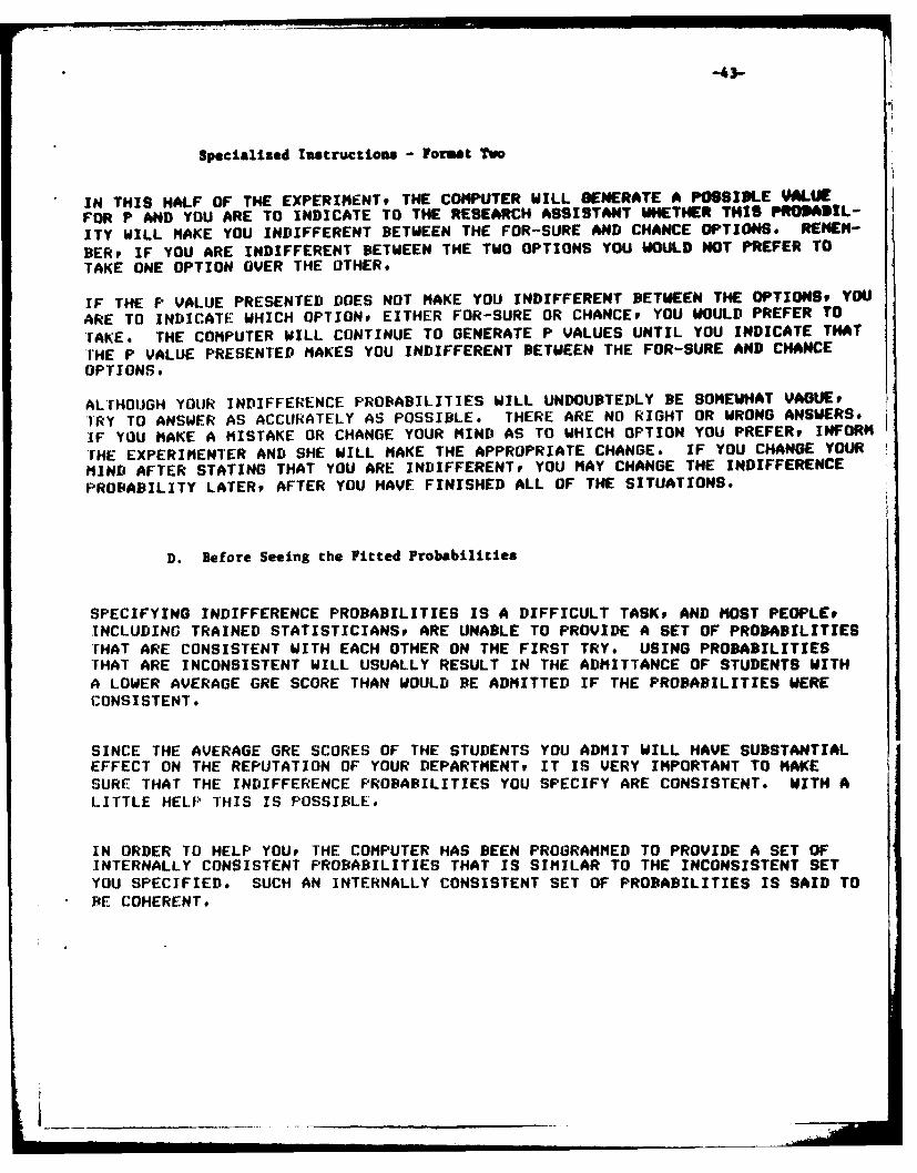
Specialized Instructions - Format Two

IN THIS HALF OF THE EXPERIMENTP THE COMPUTER WILL GENERATE A POSSIDLE MLUEFOR P AND YOU ARE TO INDICATE TO THE RESEARCH ASSISTANT WHETHER THIS PROSA DIL-

ITY WILL MAKE YOU INDIFFERENT BETWEEN THE FOR-SURE AND CHANCE OPTIONS. REMEM-

BERP IF YOU ARE INDIFFERENT BETWEEN THE TWO OPTIONS YOU WOULD NOT PREFER TO

TAKE ONE OPTION OVER THE OTHER.

IF THE P VALUE PRESENTED DOES NOT MAKE YOU INDIFFERENT BETWEEN THE OPTIONSP YOU

ARE TO INDICATE WHICH OPTION, EITHER FOR-SURE OR CHANCE, YOU WOULD PREFER TO

rAKE. THE COMPUTER WILL CONTINUE TO GENERATE P VALUES UNTIL YOU INDICATE THAT

THE P VALUE PRESENTED MAKES YOU INDIFFERENT BETWEEN THE FOR-SURE AND CHANCE

OPTIONS.

ALTHOUGH YOLiR INDIFFERENCE PROBABILITIES WILL UNDOUBTEDLY BE SOMEWHAT VAGUE,

TRY TO ANSWER AS ACCURATELY AS POSSIBLE. THERE ARE NO RIGHT OR WRONG ANSWERS.

IF YOU MAKE A MISTAKE OR CHANGE YOUR MIND AS TO WHICH OPTION YOU PREFER, INFORM

tHE EXPERIMENTER AND SHE WILL MAKE THE APPROPRIATE CHANGE. IF YOU CHANGE YOUR

MIND AFTER STATING THAT YOU ARE INDIFFERENTP YOU MAY CHANGE THE INDIFFERENCE

PROBABILITY LATER, AFTER YOU HAVE FINISHED ALL OF THE SITUATIONS.

D. Before Seeing the Fitted Probabilities

SPECIFYING INDIFFERENCE PROBABILITIES IS A DIFFICULT TASK, AND MOST PEOPLE#INCLUDING TRAINED STATISTICIANS, ARE UNABLE TO PROVIDE A SET OF PROBABILITIESTHAT ARE CONSISTENT WITH EACH OTHER ON THE FIRST TRY. USING PROBABILITIESTHAT ARE INCONSISTENT WILL USUALLY RESULT IN THE ADMITTANCE OF STUDENTS WITHA LOWER AVERAGE GRE SCORE THAN WOULD BE ADMITTED IF THE PROBABILITIES WERECONSISTENT.

SINCE THE AVERAGE GRE SCORES OF THE STUDENTS YOU ADMIT WILL HAVE SUBSTANTIALEFFECT ON THE REPUTATION OF YOUR DEPARTMENT9 IT IS VERY IMPORTANT TO MAKESURE THAT THE INDIFFERENCE PROBABILITIES YOU SPECIFY ARE CONSISTENT. WITH ALITTLE HELP THIS IS POSSIBLE.

IN ORDER TO HELP YOU, THE COMPUTER HAS BEEN PROGRAMMED TO PROVIDE A SET OFINTERNALLY CONSISTENT PROBABILITIES THAT IS SIMILAR TO THE INCONSISTENT SETYOU SPECIFIED. SUCH AN INTERNALLY CONSISTENT SET OF PROBABILITIES IS SAID TO

BE COHERENT.

l* ...

THE COMPUTER HAS FINISHED CALCULATING THE COHERENT SET OF INDIFFERENCE PROB-

ABILITIES. EXAMINE THEM CAREFULLY AND COMPARE THEM TO THE ONES YOU SPECIFIED.

IF YOU FEEL THAT THE NEW SET OF PROBABILITIES ACCURATELY REFLECTS YOURBETTING BEHAVIOR YOU MAY ACCEPT THOSE PROBABILITIES.

SINCE THE COMPUTER BASES ITS RECOMMENDED PROBABILITIES SOLELY UPON THE INDIF-

FERENCE PROBABILITIES SPECIFIED AND HAS NO REAL IDEA OF THE TRUE FEELINGS

ABOUT ORE SCORES UNDERLYING THEM, THE PROBABILITIES MAY NOT ACCURATELY REFLECTTHOSE FEELINGS.

IF YOU FEEL THAT THIS IS THE CASE YOU MAY CHANGE ANY OR ALL OF YOUR SPECIFIED

PROBABILITIES. THE COMPUTER WILL THEN GENERATE A NEW SET OF COHERENT PROB-

ABILITIES BASED ON YOUR REVISED ESTIMATES.

THE FOLLOWING TABLE SUMMARIZES THE GAMBLESP ALONG WITH THE SPECIFIED AND COM-PUTER-GENERATED INDIFFERENCE PROBABILITIES. COMPARE THE TWO SETS OF PROB-ABILITIES AND DECIDE WHETHER OR NOT THE COMPUTER-GENERATED SET ACCURATELYDESCRIBES YUR ATTITDES TOWARD THE VARIOUS TEST SCORES.

IF SOP YOU MAY DECIDE TO ACCEPT THE NEW SET OF PROBABILITIES. IF NOT, YOU MAYCHANGE SOME OR ALL OF THE ORIGINAL INDIFFERENCE PROBABILITIES YOU SPECIFIER.THINK CAREFULLY BEFORE YOU MAKE YOUR DECISION.

-'5-

FILr U11nUMT 2

The Instructions for this experiment were basically the sm as

those for Experiments I sad 3. The inotructions for ustm Fotmat four

(idif led ends-ia) my be found on page 44. The Format Three

(quartering metbod) explanation is reprinted below.

1N THIS HALF OF THE EXPERIMENT YOU WILL RE PRESENTED WITH THE FOLLOWING KIND OFTABLE# REPRESENTING ONE SITUATION, AND YOU ARE TO INDICATE WHICH OPTIONi EITHERFOR-SURE OR CHANCE, YOU WOULD PREFER TO TAKE:

FOR SURE OPTION CHANCE OPTION

I GPA I I GPA CHANCE II I I 2.5 85Z II 0.5 FOR SURE I I II I I 0.0 15Z I

ALTHOUGH YOUR RESPONSES WILL PROBABLY BE SOMEWHAT VAGUE, TRY TO ANSWER ASACCURATELY AS YOU CAN. THERE ARE NO RIGHT OR WRONG ANSWERS. IF YOU MAKE AMISTAKE OR CHANGE YOUR MIND AS TO WHICH OPTION YOU PREFER, INFORM THE RESEARCHASSISTANT AND SHE WILL MAKE THE APPROPRIATE CHANGE.

-4'-

RIRImuur 3A. Introduction - S1, RC, LC

FHE PURPOSE OF THIS EXPERIMENT IS TO STUDY GAMBLING BEHAVIOR WHEN THE OBJECT)F THE GAMBLE IS AN IMPORTANT FACTOR RELATING TO A COLLEGE STUDENT'S FUTURE)PPORTUNITIESP NAHELYt CUMULATIVE GRADE POINT AVERAGE (SPA) AT GRADUATION.

(OU WILL DE PRESENTED WITH SEVERAL SITUATIONS INVOLVING CHOICES BETWEEN GANIESIND SURE THINGS. YOU ARE TO IMAGINE THAT THE OUTCOME OF THE OPTION YOU CHOOOE4ILL RESULT IN THE FIXING OF A PARTICULAR GPA ON YOUR PERMANENT UNIVERSITYRECORD.

AHILE WE REALIZE THAT YOU ARE NOT ACCUSTOMED TO GAMBLING ON YOUR GRADE POINTiVERAGE, WE WOULD LIKE YOU TO TRY TO RESPOND AS YOU WOULD IF THESE WERE ACTUAL,ITUATIONS. CONSIDER CAREFULLY WHAT EACH GRADE POINT AVERAGE WOULD MEAN TO YOU)l GRADUATION AND HOW EACH WOULD AFFECT YOUR GOALS FOR FURTHER EDUCATION ANDz UTURE EMPLOYMENT.

!HESE GAMBLES CANNOTP OF COURSE, BE CARRIED OUT IN REAL LIFE$ HOWEVER. THE;ITUATIONS SHOULD BE MEANINGFUL TO YOU. THE PURPOSE OF THE EXPERIMENT IS TOJrUiY GAMBLING BEHAVIOR UHENl THE OUTCOMES HAVE SUBSTANTIAL IMPORTANCE RELAT--NO TO A STUDENT'S FUTURE.

S. General Instructions - SFS, LC

IN THIS EXPERIMENT YOU WILL BE PRESENTED WITH SEVERAL HYPOTHETICAL CHOICE SITU-ATIONS CONSISTING OF A FOR-SURE AND A CHANCE OPTION. THE FOR-SURE OPTIONOFFERS YOU THE CERTAINTY OF KNOWING THE OUTCOME IF YOU CHOOSE THAT OPTION.THE CHANCE OPTION OFFERS YOU A PROBABILISTIC CHANCE AT TWO POSSIBLE OUTCOMES.

* OR EXAMPLE. THE FOR-SURE OPTION COULD OFFER YOU A SPA OF 0.5. THE CHANCEOPTION COULD THEN OFFER YOU A CHANCE OF SETTING A SPA OF 2.5 WITH PROBABILITYP (WHERE P CAN BE ANY VALUE BETWEEN 5% AND 951) AND A CHANCE ON GETTING AGPA OF 0.0 WITH PROBABILITY 100-P.

.;f;SUMING THAT YOUR PREFERENCE FOR SPA'S IS 2.5 OVER 0.5 OVER 0.0 ANDASSUMING THAT YOU ARE GIVEN A CHOICE BETWEEN THE FOR-SURE AND THE CHANCEO'TIONS, YOUR DECISION AS TO WHICH OPTION YOU WOULD PREFER TO TAKE WILL DEPEND"FPON THE VALUE OF Pr THE PROBABILITY OF GETTING A SPA OF 2.5 UNDER THE,HANCE OPTION.

-47-

I.E rHANCE AND FOR-SURE OPTIONS WILL BE PRESENTED TO YOU IN SEPARATE BOXES ONtHE SCREEN AND THE PROBABILITIES ASSOCIATED WITH EACH OF THE POSSIBLE PAs INlilE CHANCE OPTION WILL BE CLEARLY HARKED.

A LITTLE THOUGHT SHOULD CONVINCE YOU THAT THE STATEMENTS IN THE FOLLOWINGTHREE PARAGRAPHS ARE TRUE. HOWEVER, THE CONCEPTS MAY SEEN SOMEWHAT DIFFICULTSO IF YOU WAVE ANY QUESTIONS OR ARE AT ALL UNSURE OF WHAT IS BEING STATED.FLEASE DO NO HESITATE TO ASK THE RESEACH ASSISTANT TO EXPLAIN THINGS MORE'LEARLY. SHE WILL BE GLAD TO CLARIFY ANYTHING YOU DO NOT QUITE UNDERSTAND.

"t R P VALUES CLOSE TO 100% YOU WILL PREFER THE CHANCE OPTION BECAUSE IT WILLIROBASLY YIELD YOU A GRADE POINT AVERAGE OF 2.5 RATHER THAN A OPA OF 0.0.IHE FOR-SURE OPTION, ON THE OTHER HAND, WILL ONLY NET YOU A OPA OF 0.5.

FOR VALUES NEAR OX, HOWEVERP YOU WILL PREFER THE SURE THING (A OPA OF 0.5)PFCAUSE THE CHANCE OPTION WILL PROBABLY YIELD YOU A GRADE POINT OF 0.0.HIS IS BECAUSE A P VALUE CLOSE TO 0% MEANS THAT THE VALUE OF 1002-P. THE

'*)JBABILITY OF GETTING A SPA OF 0.0v WILL BE NEAR 1002

IUR SOME UNIQUE INTERMEDIATE VALUE OF P YOU SHOULD BE INDIFFERENT BETWEEN'HE CHANCE AND THE FOR-SURE OPTIONS. THIS MEANS THAT WHEN P IS AT THIS VALUEfOU WOULD BE CONTENT TO LET SOMEONE ELSE DETERMINE WHICH OPTIONP EITHER,OR-SURE OR CHANCEP YOU RECEIVE.

WL ARE INTERESTED IN THIS VALUE OF P, THE INDIFFERENCE PROBABILITY, FOR EACH:;ITUATION (SET OF CHANCE AND FOR-SURE OPTIONS) WITH WHICH YOU WILL BE PRE-,tI1ED.

AIL OF THE SITUATIONS WITH WHICH YOU WILL BE PRESENTED WILL INVOLVE GPA'Sp ANDo,'E FOLLOWING SCALE FOR GRADE POINTS WILL BE USED:

~4#0=A3.0-A3.0w12.0-C1.0=D

tHESE 6PA'S ARE MEANT TO REFER TO YOUR GPA UPON GRADUATION FROM YOUR PRESENT:NVERSIIY. IN RESPONDING TO THE CHOICES THAT WILL BE

PRESENTED TO YOU,

PLEASE THINK CAREFULLY ABOUT HOW THE ENTRY OF ANY PARTICULAR OPA ON YOUR PER-MANFNT RECORD WILL AFFECT YOUR CAREER AND LIFE.

-48-

General Instructions - RC

1N THIS EXPERIMENT YOU WILL BE PRESENTED WITH SEVERAL HYPOTHETICAL CHOICE SITU-ATIONS CONSISTING OF A FOR-SURE AND A CHANCE OPTION. THE FOR-SURE OPTIONOFFERS YOU THE CERTAINTY OF KNOWING THE OUTCOME IF YOU CHOOSE THAT OPTION.THE CHANCE OPTION OFFERS YOU A PROBADILISTIC CHANCE AT TWO POSSIBLE OUTCOMES.

POR EXAMPLE, THE FOR-SURE OPTION COULD OFFER YOU A OPA OF 2.5. THE CHANCEOPTION COULD THEN OFFER YOU A CHANCE OF GETTING A OPA OF 3.5 WITH PROBABILITYP (WHERE P CAN BE ANY VALUE BETWEEN 5Z AND 95%) AND A CHANCE OF GETTING AGPA OF 1.5 WITH PROBABILTY 100%-P.

ASSUMING THAT YOUR PREFERENCE FOR 1PA'S IS 3.5 OVER 2.5 OVER 1.5 ANDASSUMING THAT YOU ARE GIVEN A CHOICE BETWEEN THE FOR-SURE AND THE CHANCEOPTIONS, YOUR DECISION AS TO WHICH OPTION YOU WOULD PREFER TO TAKE WILL DEPENDUPON THE VALUE OF P, THE PROBABILITY OF GETTING A GPA OF 3.5 UNDER THEI:HANCE OPTION.

1lIE CHANCE AND FOR-SURE OPTIONS WILL BE PRESENTED TO YOU IN BOXES ON THE

SCREEN, AND THE PROBABILITIES ASSOCIATED WITH EACH OF THE POSSIBLE OPA'S IN

THE CHANCE OPTION WILL BE CLEARLY MARKED.

A LITTLE THOUGHT SHOULD CONVINCE YOU THAT THE STATEMENTS IN THE FOLLOWING.HREE PARAGRAPHS ARE TRUE. HOWEVER, IF YOU HAVE ANY OUESTIONS OR ARE AT ALL

UNSURE OF WHAT IS BEING STATED, PLEASE DO NOT HESITATE TO ASK THE RESEACH

ASSISTANT TO EXPLAIN THINGS MORE CLEARLY. SHE WILL BE GLAD TO CLARIFY ANY-THING THAT YOU DO NOT QUITE UNDERSTAND.

FOR P VALUES CLOSE TO 100% YOU WILL PREFER THE CHANCE OPTION BECAUSE IT WILLIROBABLY YIELD YOU A GRADE POINT AVERAGE OF 3.5 RATHER THAN A OPA OF 1.5.1HE FOR-SURE OPTIONt ON THE OTHER HAND, WILL ONLY NET YOU A GPA OF 2.5.

FOR VALUES NEAR OX, HOWEVER, YOU WILL PREFER THE SURE THING (A GPA OF 2.5)BECAUSE THE CHANCE OPTION WILL PROBABLY YIELD YOU A GRADE POINT OF 1.5.THIS IS BECAUSE A P VALUE CLOSE TO OZ MEANS THAT THE VALUE OF IOOX-P, THEPROBABILITY OF GETTING A GPA OF 1.5, WILL BE NEAR 10OZ.

FOR SOME UNIQUE INTERMED1ATE VALUE OF P YOU SHOULD BE INDIFFERENT BETWEENIHE CHANCE AND THE FOR-SURE OPTIONS. THIS MEANS THAT WHEN P IS AT THIS VALUEYOU WOULD BE CONTENT TO LET SOMEONE ELSE DETERMINE WHICH OPTION, EITHERFOfR-SURE OR CHANCE, YOU RFCEIVE.

WE ARE INTERESTED IN THIS VALUE OF P, THE INDIFFERENCE PROBABILITYP FOR EACHSITUATION (SET OF CHANCE AND FOR-SURE OPTIONS) WITH WHICH YOU WILL BE PRE-

'-I NTED,

ALL OF THE SITUATIONS WITH WHICH YOU WILL BE PRESENTED WILL INVOLVE GPA'Sr ANDTHE FOLLOWING SCALE FOR ORADE POINTS WILL BE USED:

4.0=A3.0=B2.0=C1.0=DO.O=F

THESE GPA'S ARE MEANT TO REFER TO YOUR OPA UPON GRADUATION FROM YOUR PRESENTUNIVERSITY. IN RESPONDING TO THE CHOICES THAT WILL BE PRESENTED TO YOUPPLEASE THINK CAREFULLY ABOUT HOW THE ENTRY OF ANY PARTICULAR OPA ON YOUR PER-MANENT RECORD WILL AFFECT YOUR CAREER AND LIFE.

C. Procedure Specific Instructions - RC

TO HELP YOU DETERMINE WHETHER THE INDIFFERENCE PROBABILITIES YOU HAVE SPECIFIEDARE CONSISTENT WITH EACH OTHERP WE HAVE DEVISED THE FOLLOWING PROCEDURE:AFTER YOU HAVE CHOSEN TWO INDIFFERENCE PROBABILITIES, THE COMPUTER WILL PRESENTVOU WITH A TABLE WHICH DISPLAYS THESE TWO SITUATIONS AND ALSO TWO MORE SITU-A IONS FOR WHICH IT HAS DEDUCED PROBABILTIES BASED ON THE TWO YOU SPECIFIED.

THINK AGAIN OF THE SITUATION IN WHICH YOU WERE OFFERED A 'FOR-SURE' GPA OF 2.5AND A CHANCE OF GETTING A OPA OF 3s5 WITH PROBABILTY P AND OF GETTING A GPA OF2.5 WITH PROBABILITY 100Z-P. LET US IMAGINE THAT YOU SPECIFIED P TO BE 60%.NOW THINK OF A SITUATION IN WHICH YOU ARE OFFERED A 'FOR-SURE' OPA OF 3.0 VERSUSA CHANCE OF GETTING A GPA OF 3.5 WITH PROBABILITY P AND OF GETTING A GPA OF.2.5 WITH PROBABILITY 100%-P. LET US IMAGINE THAT FOR THIS SITUATION YOU CHOOSE4 P VALUE OF 65.o

SITUATIONS2 --------- 3--------- 4----

P CHANCE 3.5 3.5 3.0 3.5FOR SURE 2.5 3.0 2.5 3.0

100%-P CHANCE 1.5 2.5 1.5 1.5

P=60% P=65Z P=70% P=B6%

fOU WILL NOW BE INVITED TO EXAMINE ALL FOUR SITUATIONS AND TO DETERMINEWHETHER THE INDIFFERENCE PROBABILITIES DISPLAYED FOR EACH ARE CONSISTENTWITH YOUR VIEWS. IF YOU RECOGNIZE SOME INCONSISTENCIES YOU WILL BE ABLE TOADJUST THE P VALUES FOR ANY TWO OF THE SITUATIONS (THEREBY FIXING THE P VALUESrFuR THE OTHER TWO SITUATIONS). YOU WILL BE ASKED TO MANIPULATE THE P VALUESUNTIL YOU ARE REASONABLY SATISFIED WITH THE DISPLAYED INDIFFERENCE PROBABIL-ITIES FOR ALL FOUR SITUATIONS.

ir MAY TAKE SOME TIME TO FIND THE P VALUES THAT WILL MAKE YOU SATISFIED IN ALL)V THE SITUATIONSP SO WE HOPE THAT YOU WILL BE PATIENT AND PERSEVERING.

-50-

WE REALIZE THAT SPECIFYING INDIFFERENCE PROBABILITIES FOR ISOLATED SITUATIONSIS A DIFFICULT TASK -- EVEN TRAINED STATISTICIANS FIND IT DIFFICULT. BECAUSEIT IS HARD TO SEE HOW THE VARIOUS SITUATIONS RELATE TO EACH OTHERP THE INDIF-FERENCE PROBABILITIES FOR THEM ARE LIKELY TO BE INCONSISTENT WITH EACH OTHER.IF YO'JR FINAL GPA WERE ACTUALLY DETERMINED BY HAVING YOU PLAY THROUGH SEVERALSITUATIONS, IT WOULD BE HIGHER IF THE INDIFFERENCE PROBABILITIES FOR THEVARIOUS SITUATIONS WERE CONSISTENT WITH EACH OTHER THAN IF THEY MERE INCON-SISTENT. A SET OF CONSISTEN1 PROBABILITIES IS S4ID TO BE COHERENT.

SINCE YOUR FINAL OPA IS LIKELY TO AFFECT YOUR FUTURE OPPORTUNITIES, IT IS IN-ORTANT THAT YOU TRY TO MAKE THE INDIFFERENCE PROBABILITIES AS CONSISTENT WITH

tACH OTHER AS YOU CAN. THE PROCEDURE EXPLAINED ABOVE WAS DESIGNED TO HELPYOU IN THIS TASK. IF YOU ARE INDIFFERENT BETWEEN THE TWO OPTIONS PRESENTED.N EACH OF THE FOUR SIrUATIONS FOR THE STATED PROBABILITIES, THEN ALL OF THOSEItODIFFERENCE PROBABILIrIES WILL BE CONSISTENT WITH EACH OTHER,

Procedure Specific Instructions - LC

TO HELP YOU DETERMINE WHETHER THE INDIFFERENCE PROBABILITY YOU HAVE CHOSENACCURATELY REFLECTS YOUR VIEWS, WE HAVE PROVIDED A METHOD BY WHICH YOU CAN TEST

YOUR INITIAL JUDGMENT AGAINST A JUDGMENT IN A RELATED SITUATION,

THINK AGAIN ABOUT THE SITUATION IN WHICH YOU WERE OFFERED A 'FOR-SURE' GPA OF

0.5 VERSUS A CHANCE OF GETTING A OPA OF 2.5 WITH PROBABILITY P AND OF GETTING A

OPA OF 0.0 WITH PROBABILITY 1002-P. LET US IMAGINE THAT YOU SPECIFIED P TO

BE 50z.

THE COMPUTER PROGRAM THEN REPRODUCES THIS SITUATION (WITH P=50%) AND ALSO PRE-

SENTS YOU WITH ANOTHER TYPE OF CHOICE SITUATION CONSTRUCTED OF TWO CHANCEOPTIONS, WITH THE PROBABILITIES FOR THE NEW SITUATION DEDUCED FROM THE INDIF-FERENCE PROBABILITY YOU SPECIFIED FOR THE FIRST SITUATION.

HERE ARE THE TWO SITUATIONSGAMBLE SITUATION 1 GAMBLE SITUATION 2

I OPTION 1 OPTION 2 I I OPTION I OPTION 2 II (FOR SURE) (CHANCE) I I II 2.5 50% I 1 50% 2.5 75% 1I 0.5 I I 50% 0.5 --I 0.0 50%1 I -- 0.0 25Z I

RECALL THAT SITUATION I SAYS THAT YOU HAVE NO PREFERENCE BETWEEN GETTINGA GPA OF 0.5 FOR SURE AND TAKING A CHANCE OPTION WHICH GIVES YOU A 50% CHANCEOF GETTING A OPA OF 2.5 AND. A 50% CHANCE OF GETTING A OPA OF 0.0.

YOU ARE NOW ASKED TO DETERMINE WHETHER OR NOT YOU ARE INDIFFERENT BETWEEN THETWO OPTIONS IN SITUATION 2. NOTE THAT OPTION 2 GIVES YOU A BETTER CHANCE ATTHE MOST PREFERRED OUTCOME (2.5) BUT ALSO SOME POSSIBILITY OF GETTING THELEAST PREFERRED OUTCOME (0.0).

THERE IS NO CHANCE OF GETTING THE MIDDLE OPA (0.5). OPTION 1, ON THE OTHERHIAND, GIVES YOU A CHANCE OF GETTING THE MIDDLE OPA INSTEAD OF A CHANCE OF GET-fING THE LOWEST GPA. THIS IMPROVEMENT (ASSUMING YOU PREFER TO HAVE A CHANCE

Ot GETTING THE 0.5 TO A CHANCE OF GETTING THE 0.0),HOWEVERP IS COMPENSATED_4Y THE LOWER PROBABILITY OF GETTING THE MOST PREFERRED OPA (A 50% CHANCEVERSUS A 75% CHANCE).

-51-

YOU WILL BE ASKED TO MANIPULATE THE CHANCE OF GETTING A OPA OF 2.5 IN SITUA-TION It OPTION 2 UNTIL A)YOU ARE INDIFFERENT BETWEEN OPTIONS I AND 2 IN SITUA-TION 2 AND 9) YOU ARE ALSO INDIFFERENT BETWEEN THE FOR-SURE AND CHANCE OPTIONSIN SITUATION 1.

IT MAY TAKE SOME TIME BEFORE YOU ARE SATISFIED WITH (I.E., INDIFFERENT BETWEEN)BOTH SITUATIONSP SO WE HOPE THAT YOU WILL BE PATIENT AND PERSEVERING.

WE REALIZE THAT SPECIFYING INDIFFERENCE PROBABILITIES FOR ISOLATED SITUATIONSIS A DIFFICULT TASK -- EVEN TRAINED STATISTICIANS FIND IT DIFFICULT. BECAUSEIT IS HARD TO SEE HOW THE VARIOUS SITUATIONS RELATE TO EACH OTHERP THE INDIF-FERENCE PROBABILITIES FOR THEM ARE LIKELY TO BE INCONSISTENT WITH EACH OTHER.IF YOUR FINAL GPA WERE ACTUALLY DETERMINED BY HAVING YOU PLAY THROUGH SEVERALSITUATIONSP IT WOULD BE HIGHER IF INDIFFERENCE PROBABILITIES FOR THE VARIOUSt:ITUATIONS WERE CONSISTENT WITH E-CH OTHER THAN IF THEY WERE INCONSISTENT. ASE1 OF CONSISTENT PROBABILITIES IS SAID TO BE COHERENT.

';INCE YOUR FINAL GPA IS LIKELY TO AFFECT YOUR FUTURE OPPORTUNITIES IT IS IM-PORTANT THAT YOU TRY TO MAKE THE INDIFFERENCE PROBABILITIES AS CONSISTENT WITHLACH OTHER AS YOU CAN. THE PROCEDURE EXPLAINED ABOVE WAS DESIGNED TO HELP YOUI" THIS TASK. IF YOU ARE INDIFFERENT BETWEEN THE OPTIONS PRESENTED IN BOTHS[TUATIONS FORTHE STATED PROBABILITIES, THEN YOUR INDIFFERENCE PROBABILITIESWILL BE COHERENT.

D. Format Instructions - Direct Probability Elicitations (all procedures)

T THIS HALF OF THE EXPERIMENT THE COMPUTER WILL GENERATE THE SITUATIONS ANDYOU ARE TO TELL THE EXPERIMENTER THE VALUE OF P THAT WILL MAKE YOU INDIF-rERENT BETWEEN THE FOR-SURE AND THE CHANCE OPTIONS.

HERE IS AN EXAMPLE:FOR SURE OPTION CHANCE OPTION

I OPA I I OPA II I I 2.5 PX II 0.5 I I II I I 0.0 100X-P I

WHAT VALUE OF P MAKES YOU INDIFFERENT BETWEEN THE FOR-SURE ANDTHE CHANCE OPTIONS?

SEMFMBER, WHEN THE PROBABILITY P OF GETTING THE HIGHER OPA IN THE CHANCE OPTIONIS AT YOUR INDIFFERENCE PROBABILITYP YOU WILL LIKE THE CHANCE AND THE FOR-SUREOPTIONS EQUALLY WELL.

-52-

WE REALIZE THAT YOUR INDIFFERENCE PROBABILITIES WILL UNDOUBTEDLY BE SOMEWHATVAGUE. SINCE THERE ARE NO RIGHT OR WRONG ANSWERS, JUST TRY TO RESPOND ASDELIBERATELY, CAREFULLY AND ACCURATELY AS YOU CAN. HOWEVER. IF YOU MAKE AMISTAKE OR CHANGE YOUR MIND, DON'T WORRY, YOU WILL HAVE AN OPPORTUNITY TOCHANGE YOUR RESPONSES LATER.

Format Instructions - Modified Ends-In (all procedures)

IN THIS HALF OF THE EXPERIMENT YOU WILL BE PRESENTED WITH THE FOLLOWING KINDOF TABLE, REPRESENTING ONE SITUATIONP AND YOU ARE TO INDICATE WHICH OPTION9EITHER FOR-SURE OR CHANCE. YOU WOULD PREFER TO TAKE:

FOR SURE OPTION CHANCE OPTION-------------------------------------- -------------------------------------

I GPA I I SPA I GPAI I I I II 0.5 I I 0.0 I 2.5 1I I I I I-------------------------------------- -------------------------------------

100z 60% 40Z

IF YOU HAVE NO PREFERENCE BETWEEN THE OPTIONS, STATE THAT YOU ARE INDIFFERENT.REMEMBER. IF YOU ARE INDIFFERENT BETWEEN THE TWO OPTIONS YOU WOULD CONSENT TOTO LET SOMEONE ELSE CHOOSE WHICH OPTION, EITHER FOR-SURE OR CHANCE. YOU RECEIVE.ALTHOUGH YOUR REPONSES WILL UNDOUBTEDLY BE RATHER VAGUE, TRY TO ANSWER ASACCURATELY AS YOU CAN. THERE ARE NO RIGHT OR WRONG ANSWERS. IF YOU HAKE AMISTAKE OR CHANGE YOUR MIND AS TO WHICH OPTION YOU PREFER, INFORM THE RESEARCHASSISTANT AND SHE tILL MAKE THE APPROPRIATE CHANGE. YOUR FIRST SITUATIONrOLLOWS.

3. Procedure Specific Instructions - SFS

SPECIFYING INDIFFERENCE PROBABILITIES IS A DIFFICULT TASK, AND MOST PEOPLE,INCLUDING TRAINED STATISTICIANS. ARE UNABLE TO PROVIDE A SET OF PROBABILITIESTHAT ARE CONSISTENT WITH EACH OTHER ON THE FIRST TRY. USING PROBABILITIESTHAT ARE INCONSISTENT WILL USUALLY RESULT IN THE APPEARANCE OF A LOWER FINALOPA ON YOUR PERMANENT RECORD THAN WOULD APPEAR IF THE PROBABILITIES WERECONSISTENT.

ZSINCE YOUR FINAL GRADE POINT AVERAGE WILL GREATLY AFFECT YOUR OPPORTUNITIES FORTHE FUTURE. IT IS VERY IMPORTANT TO MAKE SURE THAT THE INDIFFERENCE PROB-ABILITIES YOU SPECIFY ARE CONSISTENT. WITH A LITTLE HELP THIS IS POSSIBLE.

IN ORDER TO HELP YOU. THE COMPUTER HAS BEEN PROGRAMMED TO PROVIDE A SET OFINTERNALLY CONSISTENT PROBABILITIES THAT IS SIMILAR TO THE INCONSISTENT SETYOU SPECIFIED. SUCH AN INTERNALLY CONSISTENT SET OF PROBABILITIES IS SAID TODE COHERENT.

-53-

SIT BACK AND RELAX FOR A FEW MINUTES WHILE THE COMPUTER MAKES THE NECESSARY

CALCULATIONS.

thE COMPUTER HAS FINISHED CALCULATING THE COHERENT SET OF INDIFFERENCE PRO9-

ABILITIES. EXAMINE THEM CAREFULLY AND COMPARE THEM TO THE ONES YOU SPECIFIED.

IF YOU FEEL THAT THE NEW SET OF PROBABILITIES ACCURATELY REFLECTS YOUR

PETTING BEHAVIOR YOU MAY ACCEPT THOSE PROBABILITIES.

';INCE THE COMPUTER BASES ITS RECOMMENDED PROBABILITIES SOLELY UPON THE INDIF-

FERENCE PROBABILITIES SPECIFIED AND HAS NO REAL IDEA OF THE TRUE FEELINGS

ABOUT GRADE POINT AVERAGES UNDERLYING THEM, THE PROBABILITIES MAY NOT ACCU-

kATELY REFLECT THOSE FEELINGS.

IF YOU FEEL THAT THIS IS THE CASE YOU MAY CHANGE ANY OR ALL OF YOUR SPECIFIED

PROBABILITIES. THE COMPUTER WILL THEN GENERATE A NEW SET OF COHERENT PROB-

ABILITIES BASED ON YOUR REVISED ESTIMATES.

THE FOLLOWING TABLE SUMMARIZES THE GAMBLES, ALONG WITH THE SPECIFIED AND COM-

PUTER-GENERATED INDIFFERENCE PROBABILITIES. COMPARE THE TWO SETS OF PROB-

ABILITIES AND DECIDE WHETHER OR NOT THE COMPUTER-GENERATED SET ACCURATELY

DESCRIBES YOUR ATTITUDES TOWARD THE VARIOUS GRADE POINT AVERAGES.

IF SO, YOU MAY DECIDE TO ACCEPT THE NEW SET OF PROBABILITIES. IF NOT, YOU MAY

:HANGE SOME OR ALL OF THE ORIGINAL INDIFFERENCE PROBABILITIES YOU SPECIFIED.

!-HINK CAREFULLY BEFORE YOU MAKE YOUR DECISION.

;TTUATION FOR CHANCE INDIFF. P

NO. SURE P 100%-P SPEC'D COMP

1 0.50 1.00 0.00 50% 52%

2 L.00 2.00 0.00 50% 53%

3 1.50 2.50 0.50 50% 54X

4 2.00 2.50 1.50 50% 54%

5 2.50 4.00 1.00 65Z 62%

6 3.00 3.50 2.50 55% 53%

7 3.50 4.00 3.00 70% 69%

8 100 1.50 0.50 50% 51% OPTIONS

9 1.50 2.00 1.00 50% 52Z 1. MODIFY SPEC'D P'S

10 1.50 3.00 0.00 60% 57% 2. ACCEPT COMP P'S

11 2.00 3.00 1.00 50% 56%

12 2,00 4.00 0.00 70% 63%

13 2.50 3.00 2.00 50% 52%

14 2.50 3.50 1.50 55% 56%

15 3.00 4.00 2.00 55% 62%

OPTION?

-54-

APPENDIX C - Questionnaire

1. Wave you at any time unsure of what was expected of you?If so, when?

2. How could the directions have been changed so as to alleviatethe above problem?

3. Are there any coments you would like to make about theexperiment or the experimenter?

4. (Experiment 3 only) Please give some indication of how usefuleach GPA in the followift scale is to you. The utility (usefulnessor worth) of a CPA of 0.0 is assumed to be 0 while that of a CPAof 4.0 is 100. Please specify intermediate values for the otherCPAs.

CPA utility to you

0.0 0

0.5

1.0

1.5-

2.0

2.5

3.0

3.5

4.0 100

Appendix D

Results Tables for Experiment 3

TABLE 4

Overall Mean Absolute Errors for Forty Subjects with Breakdowa

by Procedure and Sex

MALES FIMALES

RC SFS LC KC SFs LC

.6574 .7736 .5976 .1311 .2317 .2405

1/4 .2972 .3991 .3883 .1927 .0555 .4447

.4372 .6445 .3433 .4662 .3237 .6073

.3383

Format _Order

.8540 .2099 .5727 .2037 .3917 .3550

S.4051 .4936 .2479 .3516 .3026 .5020

4.3105 .5067 .2180 .4409 .3342 .4059

.4188 .6506 .6S16

x=.4803 x-.5046 x-.3938 x-.2978 x-.3285 x-.4624n-7 n-6 n-6 n-6 n8 n-n7

Grand Mean (H) - .4065

Procedure: Sex:

xRC - .3923 (n - 13) xm - .4554 (n 19)x~~( 02 (n9)14S - .4021 ( - 14) - .3623 (a - 21)

xLC .4295 (n - 13)

-56-

TABLE 5

Average Mean Absolute Errors for Forty Subjects Broken Down

by Procedure, Format and Sex

FOMT 1

tC SFS LC

Males x - .5213 x - .4931 x - .3751 x- .4662

n- 7 n 6 n- 19

Females x - .3085 x - .3112 x - .4589 x, - .3597

n-6 naS n-7 -,21

xR a .4231 XSFS - .3892 X - .4202 x1 ..103

n- 13 n- 14 n- 13 n- 40

FOfMAT 4

RC SFS LC

Males x - .4275 x - .4974 x - .4122 xK - .4447

n- 7 n 6 n 6 n- 19

Females x- .2846 x - .3469 x -. 4615 xF .3673

_ -6 -a8 -"7 , -21

- .3615 x - .4133 x - .4387 x4 - .4040

n - 13 n- 14 n- 13 n - 40

TABL 6

Differeaces In MA (Format 1 MAE - Format 4 MAE)

for Forty Subjects with Breakds by

Procedure and Sex

RC SPS LC

-.2174 .2592 .0490

.0698 -.2262 .0262

.0015 .2177 -.1275

Males .0564 -.3650 .0305

.0181 .0850 1289 -.0408

n - 19 -.1339 -.0676 -.15"

.7571

x - .0884 z - -.0088 = -.0371

n-7 n-6 n-6

-.0079 -.0055 -.0169

-.0887 -.0618 -.1135

.1241 .0515 .1523

Females .1431 .0282 .0049

xF - -.0075 -.0372 .0049 .0135

n - 21 .0105 -.0302 -.1365

-.1079 .0779

-.1650

.0240 x - -.0357 x- -.0026

n=6 n-S n -7

M-.0046 N -40

- .0587 XSFS --.0242 x - -.0185

n- 13 n- 14 n-13

-58-

TABLE 7

Greatest Absolute Differences in Utilities (GAVU) for FortySubjects with Breakdowns by Procedure, Format and Sex

MALES FEMALES

IC LC SFS RC LC SFs

.2129 .1642 .6096 4039 .1850 .5449

.1170 .3699 .3601 1494 .4958 .5193Forlmat1 .1757 .2361 .5596 5620 .4798 .1872

.2343

x - .685 x -. 2369 x -A-40S x-m. 1 718 x -. 16 x -. 714

.7205 .2477 .3635 2844 .8104 .3758

.2763 .3210 .1178 ,2070 .1759 .4199

Format .2145 .5064 .2234 .1380 .2826 .65994

.1153 .2940 .2165

1316___ u.33841 n u2J491 x T298 1 x .3108 %-..P67

Grand Mean (M) - .3384

Procedure:

Qxuc- .2751 (n - 13)

Xc- .3514 (n- 13)

i - .3848 (n - 14)SFs

Format:

XFl .3456 (n a 19)

x 74 .3319 (n - 21)

Sex:* .3111 (n- 19)

X, - .3631 ( - 21)

-59-

TABLE 8

Tvo-way Summary Tables for Dependent Variable - GADU

A. Summary Table for Procedure by Format

IC LC SFS

Format x - .2701 x - .3218 x - .4307 x1' .3456

Sn- 6 n- 6 n-7 n-19

Format x - .2794 x - .3769 x - .3388 x1 4 - .3319

4 n- 7 n- 7 n- 7 a-21

x Rc .2751 LC - .3514 xSFs- .3848

a-1 3 n-13 n- 14

B. Summary Table for Sex by Format

MALES FIMALES

Format x - .3117 x - .3762 'I ' .3436

n = 9 - 10 n- 19

Format x - .3106 x -. 3513 'F " .3319

4 n - 10 n- 11 n 21

x1 - .3111 xF - .3631

n- 19 n - 21

C. Sumary Table for Procedure by Sex

RC LC SF1

Males x - .2617 x -. 3076 x - .3723 -N .3111

n-=7 n6 n -6 au 19

Females .2908 -. 3891 a-.3940 -. 3631

n6 n 7 a-S 21

xi - .2751 3 14 m 3

n-13 a- 13--'

-60-

Figure I

Procedure X Foruest X Sex Interaction

For The GADU Variable

M~.s FevwAts

A- A

It

sef-C5 . LC SFS

PrOCCAOMe Procxe.

- rwwA L.

-61-

References

Coombs, C. IH. Portfolio theory and the measurement of risk. In M.

F. Kaplan & S. Schwartz. lHuman Judgment and decision processes.

New York: Academic Press, Inc., 1975, 63-85.

Fischhoff, B., Slovic, P., & Lichtenstein, S. Fault trees: Sensitivityof estimated failure probabilities to problem representation.Technical report PTR-1042-77-8, 1977.

Fischhoff, B., Slovic, P.. 4 Lichtenstein, S. Knowing what you want:Measuring labile values. Appearing in T. Wallsten (Ed.).Counitive Processes in Choice and Decision Behavior. Hillsdale,New Jersey: Erlbaum, in press.

Ilogarth. R.I. Cognitive processes and the assessment of subjectiveprobability distributions. Journal of the American StatisticalAssociation. 1975, 70, 350, 271-289.

Isoacs, G. L., & Novick, H. R. Computer assisted data analysismonitor, 1978.

Kahneman, D., & Tversky, A. Prospect theory: An analysis of decisionunder risk. Econometrics. 1979, 47,263-291.

Kahneman, D., & Tversky, A. Subjective probability: A judgmentof representativeness. Cognitive Psychology. 1972, 3,430-454.

Keeney, R. L., & Raiffa, H. Decisions with multiple objectives:Preferences and value tradeoffs. New York: John Wiley &Sons, 1976.

Krantz, D. If.. Luce, R. D., Suppes, P., & Tversky, A. Foundationsof Measurement, Vol. 1. Nev York: Academic Press. 17iT.

Hosteller, F., & Nogee, P. An experimental measuremt of utility.Journal of Political Ecoltowm. 1951, 59, 5, 371-404.

McDaniel, S. D., Halter, A. N., A Hartford, D. L. Grade utility:

a new noncognitive factor in academic prediction. Educationaland Psychological M*esurge t. 1961, 21. 3. 62l-62.

-62-

Novick. N. R., Chuang, D., 6 DeKeyrel, D. Local and regionalcoherence utility assessment procedures. Trabajos de Estadistica,in press, 1981.

Novick, M. R., Isaacs, G. L., Hamer, R., Chen, J., Chuang, D.,Woodworth, G., Molenaar, I., Lewis, C., & Libby, D. Computer-assisted data analysis monitor. 1980.

Novick, M. R., & Lindley, D. V. Fixed-state assessment of utilityfunctions. The Journal of the American Statistical Association,1979, 74, 306-311.

Novick, M. R., & Lindley, D. V. The use of more realistic utilityfunctions in educational applications. Journal of ductiosal

Measurement. 1978, 15, 181-192.

Payne, J. W. Alternative approaches to decision making under risk:moments versus risk dimensions. Psycboloical 401lleIa. 1973.80, 6, 439-453.

Raiffa, H., & Schlifer, R. Applied statistical dwcisitM thoe.Boston: Graduate School of Duaiess Adifaitra eam lavUniversity, 1961.

Schlsifer, K. Computer proarMs for leGMeaM d ISo easnests.Boston: Graduate School of Business AdmioistratIm a"rvedUniversity, 1971.

Sehlaifer, R. Probability ad statLstis fer bs/mans dWislms:An introduction to mnagerial sefmemics uVe unsetaCY.New York: McGraw-Hill Book Co., Inc., 1959.

Slovic, P. From Shakespeare to Simo: Spoculatie - and smevidence - about man's ability to process Imfotmatiea.Or&&n Research Institute eseareh Bllatin. 1972, "3, (2) 1-29.

Slovic, P., Fischoff, B., & Lichtenstein, S. Behavioral decisiontheory. Annual Review of Psychology. 1977, 28, 1-39.

Spettier, C. S., & Stal von Holstein, C-A. S. Probabilityencoding in decision analysis. Management Science. 1975,22, 340-358.

Swain, R. 0. Utility theory--insights into risk taking. HarvardBusinss Review. 1966, 44, 6, 123-136.

-63-

Torgerson. V. S. Thery and methods of scaling. NMw York: JohnWiley & Sons, Inc., 1956.

Tversky, A. On the elicitation of preferences: Descriptive andprescriptive considerations. Twub. z. Bell, L. L. Keemey,H. Raiffa (Us.), Conflictia objectives In decaoms. Chichester:John Wiley & Sons, 1977, 209-ZZZ.

Tversky, A., & Kahueman, 0. Judgment under uncertainty: Heuristics andbiases. Science. 1974, 185, 1124-1131.

Vertinsky, I., & Wong, E. Eliciting preferences and the constructionof indifference maps: a comparative empirical evaluation of tvomeasurement methodologies. Socio-Sco.muIc Planning Sciences.1975, 9, 15-24.

Viek, C.A.J. Coherence of lumen Judgment in a limited probabilisticenvironment. Organiational Sehavlor and fum Perfo some.1973, 9, 460-481.

von Neumann, J., 6 Morgenstern, 0. Theory of iames and economicbehavior. Princeton: Princeton University Press, 1953.

IOWA/NOVICK November 6, 1960 Page 1

Navy Navy

Dr. Ed Aiken 1 Dr. Patrick R. HarrisonNavy Personnel PAD Center Psychology Courn DirectorSan Diego, CA 92152 LEADERSHIP & LAW DEPT. (7b)

DIV. OF PROFESSIONAL DEVELORNNTDr. Jack R. Borsting U.S. NAVAL ACADEIYProvost & Acadmic Dean ANNAPOLIS, ND 21402U.S. Naval Postgraduate SchoolMonterey, CA 93940 1 Dr. Norman J. Kerr

Chief of Naval Teohnical TrainingDr. Robert Breaux Naval Air Station Memphis (75)Code N-711 Millington, TN 38054NAVTRAEQUIPCENOrlando, FL 32813 1 Dr. Wi11im L. Maloy

Principal Civilian Advisor forChief of Naval Education and Training Education and Traiing

Liason Office Naval Training Command, Code OOAAir Force Homan Resource Laboratory Pensacola, FL 32508Flying Training DivisionWILLIAMS AFB. AZ 85224 1 Dr. Kneale Marshall

Scientific Advisor to DCNO(MFT)Deputy Assistant Secretary of the Navy OPOIT

(Manpower) Washington DC 20370Office of the Assistant Secretary of

the Navy (Manpower, Reserve Affairs,1 CAPT Richard L. Martin, USNand Logistics) Proapectlve Coemnding Officer

Washington, DC 20350 USS Carl Vinson (CN-70)Newport News Shipbuilding and Drydock Co

Dr. Richard Elater Newport News, VA 2360?Department of Administrative SciencesNaval Postgraduate School 1 Dr. James McBrideMonterey, CA 93940 Navy Personnel PAD Center

San Diego, CA 92152DR. PAT FEDERICONAVY PERSONNEL R&D CENTER 1 Dr Willim MontagueSAN DIEGO, CA 92152 Navy Personnel R&D Center

San Diego, CA 92152Mr. Paul FoleyNavy Personnel R&D Center 1 Ted N. I. TellenSan Diego, CA 92152 Technical Information Office, Code 201

NAVY PERSONNEL R&D CENTERDr. John Ford SAN DIEGO, CA 92152Navy Personnel R&D CenterSan Diego, CA 92152 1 Library, Code I01L

Navy Personnel RD CenterDr. Henry N. Halff San Diego, CA 92152Department of Psychology,C-009University of California at San DiegoLa Jolla, CA 92093

IOWA/NOVICK November 6. 1980 Pae 2

Navy Navy

6 Commanding Officer 1 Dr. Robert G. SmithNaval Research Laboratory Office of Chief of Naval OperationsCode 2627 OP-987HWashington, DC 20390 Washington, DC 20350

Psychologist 1 Dr. Alfred F. modaON Branch Office Training Analysis & Evaluation GroupBldg 114, Section D (TAEG)666 Summer Street Dept. of the NavyBoston, MA 02210 Orlando, FL 32813

Psychologist 1 Dr. Richard SorensenOUR Branch Office Navy Personnel R&D Center536 S. Clark Street San Diego, CA 92152Chicago, IL 60605

1 W. Gary ThomsonOffice of Naval Research Naval Ocean Systems CenterCode 437 Code 7132800 N. Quincy SStreet San Diegc, CA 92152Arlington, VA 22217

1 Dr. Donald Weitman5 Personnel & Training Research Programs Code 54 WZ

(Code 458) Department of Administrative SciencesOffice of Naval Research U. S. Naval Postgraduate SchoolArlington, VA 22217 Monterey, CA 9390

Psychologist I DR. MARTIN F. WISMOFFOUR Branch Office NAVY PERSONNEL R& 0 CETER1030 East Green Street SAN DIEGO, CA 92152Pasadena, CA 91101

Office of the Chief of Naval OperationsResearch Develojment & Studies Branch

(OP-115)Washington, DC 20350

I LT Frank C. Petho, MSC, USN (Ph.D)Code L51Naval Aerospace Medical Research LaboratPensacola, FL 32508

1 r. Arnold RubensteinNaval Personnel Support TeohnologyNaval Material Comand (08T244)loom 104, Crystal Plei IS2221 Jefferson Davis RighusyArlington, VA 20360

. ..... -

IOWA/NOVICK November 6, 1980 Page 3

Army Army.

1 Technical Director 1 Dr. Joseph WardU. S. Army Research Institute for the U.S. Army Research Institute

Behavioral and Social Sciences 5001 Eisenhower Avenue5001 Eisenhower Avenue Alexandria, VA 22333Alexandria, VA 22333

I HO USAREUE & 7th ArmyODCSOPSUSAAREUE Director of GED

, APO New York 091103

1 DR. RALPH DUSEKU.S. ARMY RESEARCH INSTITUTE5001 EISENHCOWER AVENUEALEXANDRIA, VA 22333

1 Dr. Myron FischlU.S. Army Research Institute for the

Social and Behavioral Sciences5001 Eisenhower AvenueAlexandria, VA 22333

1 Dr. Harold F. O'Neil, Jr.Attn: PERI-OKArmy Research Institute5001 Eisenhower AvenueAlexandria, VA 22333

1 Mr. Robert RossU.S. Army Research Institute for the

Social and Behavioral Sciences5001 Eisenhower AvenueAlexandria, VA 22333

1 Dr. Robert SasuorU. S. Army Research Institute for the

Behavioral and Social Sciences5001 Eisenhower AvenueAlexandria, VA 22333

1 CommandantUS Army Institute of AdministrationAttn: Dr. SherrillFT Denjmln Harrison, IN 46256

1 Dr. Frederick SteinheiserU. S. Army Reserch Institute

50n1 Eisenhower AvenueAlexandria, VA 22333

IOWAJNOVICK November 6, 1990 page 4

Air Force Marines

1 Air Force Human Resources Lab 1 H. William GreenupAFHRL/MPD Education Advisor (E031)Brooks AFB, TX 78235 Education Center, MCDEC

Quantico, VA 221341 Air University Library

AUL/LSE 76/443 1 Director, Office of Manpower UtilizationMaxwell AFB, AL 36112 HQ, Marine Corps (MPU)

BCB, Bldg. 20091 Dr. Earl A. Alluisi Quantico, VA 22134

HQ, AFHRL (AFSC)Brooks AFB. TX 78235 1 DR. A.L. SLAFKOSK¥

SCIENTIFIC ADVISOR (CODE RD-1)1 Dr. Genevieve Haddad HQ, U.S. MARINE CORPS

Program Manager WASHINGTON, DC 20380Life Sciences DirectorateAFOSRBolling AFB, DC 20332

1 Dr. Ros L. Morgan (AFHRL/LR)Wright -Patterson AFBOhio 45433

1 Research and Measurment DivisionResearch Branch, AFNPC/MPCYPRRandolph AFB, TX 781148

1 Dr. Malcolm BeeAFHRL/MPBrooks AFB, TX 78235

1 Dr. Marty RockwayTechnical DirectorAFHRL(OT)W1llas AFB, AZ 58224

1 Jack A. Thorp, Maj., USAFLife Sciences DirectorateAFOSRBollina AFB, DC 20332

IOWA/NOVICK November 6, 1980 Page 5

CoastGuard Other DoD

Mr. Thomas A. Warm 12 Defense Technical Information CanterU. S. Coast Guard Institute Cameron Station, Bldg 5P. 0. Substation 18 Alexandria, VA 22314Oklahoma City, OK 73169 Attn: TC

1 Dr. Dexter FletcherADVANCED RESEARCH PROJECTS AGENCY1400 WILSON BLVD.

ARLINGTON, VA 22209

1 Dr. William Graham

Testing DirectoratePEPCCH/MEPCT-PFt. Sheridan, IL 60037

1 Military Assistant for Training andPersonnel Technology

Office of the Under Secretary of Defensefor Research & Egineering

Room 3D129, The PentagonWashington, DC 20301

1 MAJOR Wayne Sellman, USAFOffice of the Assistant Secretary

of Defense (MR&L)38930 The PentagonWashington, DC 20301

1 HEAD, SECTION ON MEDICAL EDUCATIONUNIFORMED SERVICES UNIV. OF THE

HEALTH SCIENCES6917 ARLINGTON ROADBETHESDA, MD 200114

ICOA/NOVICK November 6, 1990 Page 6

Civil Govt Non Gcvt

Dr. Susan Chipman 1 Dr. Erling B. AndersenLearning and Development Department cf StatiaticsNational Institute of Education Studlestrede 61200 19th Street NW 1455 CopenhagenWashington, DC 20208 DEIARK

Dr. Joseph 1. Lipson 1 1 psychological research unitSED W-638 Dept. of Defense (Army Office)National Science Foundation Campbell Park OfficesWashington, DC 20550 Canberra ACT 2600, Australia

Dr. John Hays 1 Dr. Isaac BejarNational Institute of Education Educational Testing Service1200 19th Street NW Princeton, NJ 081450

Washington, DC 202081 Dr. Werner Birke

Dr. Arthur elmed DezWPs im StreitkraefteamtNational Intitute of Education Postfach 20 50 031200 19th Street NW D-5300 Bonn 2Washington, DC 20208 WEST GERMANY

Dr. Andrew R. Molnar 1 Dr. Nicholas A. BondScience Education Dev. Dept. of Psychology

and Research Sacramento State CollegeNational Science Foundation 600 Jay StreetWashington, DC 20550 Sacramento, CA 95819

Personnel R&D Center I Dr. David G. BowersOffice of Personnel Managment Institute for Social Research1900 E Street 1W University of MichiganWashington, DC 20415 P. 0. Box 1248

Ann Arbor, MI 48106

Personnel R&D Center 1 Dr. Robert BrennanOffice of Personnel Management Merican College Testing Programs1900 E Street NW P. 0. Box 168Washington, DC 20415 Iowa City, IA 52240

Dr. Frank Withrow 1 DR. C. VICTOR BUNDERSONU. S. Office of Education WICAT INC.400 Maryland Ave. SW UNIVERSITY PLAZA, SUITE 10

Washington, DC 20202 1160 SO. STATE ST.OREM, UT 84057

Dr. Joseph L. Young, DirectorMemory & Cognitive Processes 1 Dr. John B. CarrollNational Science Foundation Psychometric LabWashington, DC 20550 Univ. of No. Carolina

Davie Hall 013AChapel Hill, NC 275114

IOWA/UOVICK November 6, 1980 Page 7

Non Govt Non Govt

I Charles Myers Library I Dr. Leonard FeldtLivingstone House Lindquist Center for MeasurmentLivingstone Road University of IowStratford Iowa City, IA 52242London E15 2LJENGLAND 1 Dr. Richard L. Ferguson

The American College Testing ProgramDr. Kenneth E. Clark P.O. Box 168College of Arts & Sciences Iowa City, IA 52240University of RochesterRiver Campus Station 1 Dr. Victor FieldsRochester, NY 14627 Dept. of Psychology

Montgomery College1 Dr. Norman Cliff Rockville, MD 20850

Dept. of PsychologyUniv. of So. California I Univ. Prof. Dr. Gerhard FischerUniversity Park Liebiggasse 5/3Los Angeles. CA 90007 A 1010 Vienna

AUSTRIADr. William E. CoffnanDirector, Iowa Testing Programs I Professor Donald Fitzgerald334 Lindquist Center University of New EnglandUniversity of Iowa Armidale, New South Wales 2351lowa City, IA 52242 AUSTRALIA

Dr. Meredith P. Crawford 1 Dr. Edwin A. FleishmanAmerican Psychological Association Advanced Research Resources Organ.1200 17th Street, N.W. Suite 900Washington, DC 20036 4330 East West Highway

Washington, DC 20014Dr. Hans CrombagEducation Research Center 1 Dr. John R. FrederikienUniversity of Leyden Bolt Beranek & NewmanBoerhaavelaan 2 50 Moulton Street2334 EN Leyden Cambridge, MA 02138The NETHERLANDS

1 DR. ROBERT GLASERDr. Bumanuel Donchin LRDCDepartment of Psychology UNIVERSITY OF PITTSBURGHUniversity of Illinois 3939 O'HARA STREETChampaign, IL 61820 PITTSBURGH, PA 15213

LCOL J. C. Eggenberger 1 Dr. Ron HambletonDIRECTORATE OF PERSONNEL APPLIED RESEARC School of BducationNhTIONAL DEFENCE HQ University of assechusetta101 COLONEL BY DRIVE Amherst, MA 01002OTTAWA. CANADA K1A 01(2

IOWA/NOVICK November 6. 1960 Page 8

Non Govt Non Govt

Dr. Chester Harris 1 Dr. Michael LevineSchool of Education Department of Educational PsychologyUniversity of California 210 Education Didg.Santa Barbara, CA 93106 University of Illinois

Champaign, IL 61801Dr. Lloyd HumphreysDepartment of Psychology 1 Dr. Charles LewisUniversity of Illinois Facultelt Sociale WetenschappenChampaign, IL 61820 Rijksuniversitelt Groningen

Oude BoteringestraitLibrary GroningenHumRRO/Weastern Division NETHERLANDS27857 Berwick DriveCamel, CA 93921 1 Dr. Robert Linn

College of EducationDr. Steven Hunka University of IllinoisDepartment of Education Urbana, IL 61801University of AlbertaEdmonton, Alberta 1 Dr. Frederick H. LordCANADA Educational Testing Service

Princeton, NJ 08540Dr. Earl MintDept. of Psychology 1 Dr. Gary MrcoUniversity of Washington Educational Testing ServiceSeattle, WA 98105 Princeton, NJ 08450

Dr. Huynh Huynh I Dr. Scott MaxwellCollege of Education Department of PsychologyUniversity of South Carolina University of HoustonColumbia, SC 29208 Houston, TX 77004

Dr. Douglas H. Jones 1 Dr. Samuel T. MayoNo T-255 Loyola University of ChicagoEducational Testing Service 820 North Michigan AvenuePrinceton, NJ 08450 Chicago, IL 60611

Professor John A. Keats 1 Dr. James A. PaulsonUniversity of Newcastle Portland State UniversityAUSTRALIA 2308 P.O. Box 751

Portland, ON 97207Dr. Mazie KnerrLitton-Mellontcs 1 MR. LUIGI PETRULLOBox 1286 2431 N. EDGEWOOD STREETSpringfield, VA 22151 ARLINGTON, VA 22207

Mr. Marlin 1Kroger 1 DR. DIANE M. RANSZT4-IEE1117 Via Goleta R-K RESEARCH & S1STEM 09SIONPalos Verdes Estates, CA 90274 3947 RIDGEMONT DRIVE

MALIBU, CA 90265

IOVANOVICK bvmber. 6, 190 Page 9

Non Govt Non Govt

1 MINRAT M. L. RAUCH 1 Dr. Kawo aisomaMP II 4 University or TohokuBUNDESHINISTERIU ER VERTEIDIGUNG Department of Educational PsychologyP0STFACH 1328 Kawauchi, Sendai 9800-53 BONN 1, GEMNANY JAPAN

1 Dr. Hark D. Reckase 1 Dr. Richard 3cowEducational Psychology Dept. School of EduoationUniversity of issouri-Columbis Stanford University4 Hill Hall Stanford, CA "305Columbia, NO 65211

1 Dr. Robert Sternberg1 Dr. Andrew N. Rose Dept. of Psychology

American institutes for Research Yale University1055 Thomas Jefferson St. Nd Box 11A, Yale StationWahington, DC 20007 New Haven, CT 06520

1 Dr. Leonard L. Rosenbaum, Chairman 1 DR. PATRICK SUPPESDepartment of Psychology INSTITUTE FOR NATHEMATICAL STUDIES INHontgomery College THE SOCIAL SCIENCESRockville, MD 20850 STANFORD UNIVERSITY

STANFORD, CA 9143051 Dr. Ernst Z. Rothkopf

Bell Laboratories 1 Dr. Hariharan Swasinathan600 Mountain Avenue Laboratory of Psychometric andHurray Hill, NJ 07974 Evaluation Research

School of Education1 Dr. Lawrence Rudner University of Hassachusetts

403 Elm Avenue Amherst, MA 01003Takoma Park, MD 20012

1 Dr. Brad Sympion1 Dr. J. Ryan Psychometric Research Group

Department of Education Educational Testing ServiceUniversity of South Carolina Princeton, NJ OSAlColumbia, SC 29208

i Dr. Kikumi Tatauoka1 PROF. FUNIND SAHEJIHA Computer Booed Education Research

DEPT. OF PSYCHOLOGY LaboratoryUNIVERSITY OF TENNESSEE 252 Engineering Research LaboratoryKNOXVILLE, TN 37916 University of Illinois

Urbana, IL 618011 Committee on Cognitive Research

, S Dr. Lonnie R. Sherrod 1 Dr. David himn* Social Science Research Council Department of Psychology

605 Third Avenue University of KansasNew York, NY 10016 Lawrenoe, KS 66041

IOAWOVICI Nbovmber 6# 1980 P88e 10

Von €vvt

Dr. J. UlmerPereeptronloa. Ine.6271 Varlel AvoewWoodland alls, CA 91364

Dr. Voward ValnerBureau of Social SCience Research1990 H Street, N. M.

Washington, DC 20036

DR. THONAS WALLSTNPSYCHOMETRIC LABORATORYDAVIE HALL 013AUNIVERSITY OF NORTH CAROLCHAPEL HILL, NC 27514

IDr.. Devid J. VelN660 Elliott HallIiversity of Hinnesota75 E. River RoadMinneapolls, KI 55455

DR. SUSAN E. WHITELYPSYCHOLOGY DEPARTMENTUNIVERSTY OF rANSA3LAWRENCE, KANSAS 66044

I olfgang Wildgru*Streitkraeft*ntRBx 20 50 03D-5300 Bonn 211? GEMANY

Dr. J. Arthur VoodwardDepartment of PsyohologyUniversity of CallfornlaLos Angeles, CA 90024

Dr. Karl ZinnCenter for resroh on Learnin

and TeaohingUniversity of MIchilan

Am Arbor, 1I 48104

oS