Zero-Inflated Poisson and Binomial Regression with Random Effects

BIOMETRICS 56, 1030-1039 December 2000

Zero-Inflated Poisson and Binomial Regression with Random Effects: A Case Study

Daniel B. Hall Department of Statistics, University of Georgia, Athens, Georgia 30602-1952, U.S.A.

ernail: [email protected]

SUMMARY. In a 1992 Technometrzcs paper, Lambert (1992, 34, 1-14) described zero-inflated Poisson (ZIP) regression, a class of models for count data with excess zeros. In a ZIP model, a count response variable is assumed to be distributed as a mixture of a Poisson(X) distribution and a distribution with point mass of one at zero, with mixing probability p . Both p and X are allowed to depend on covariates through canonical link generalized linear models. In this paper, we adapt Lambert’s methodology to an upper bounded count situation, thereby obtaining a zero-inflated binomial (ZIB) model. In addition, we add to the flexibility of these fixed effects models by incorporating random effects so that, e.g., the within-subject correlation and between-subject heterogeneity typical of repeated measures data can be accommodated. We motivate, develop, and illustrate the methods described here with an example from horticulture, where both upper bounded count (binomial-type) and unbounded count (Poisson-type) data with excess zeros were collected in a repeated measures designed experiment.

KEY WORDS: Excess zeros; EM algorithm; Generalized linear mixed model; Heterogeneity; Mixed effects; Overdispersion; Repeated measures.

1. Introduction Count data with many zeros are common in a wide variety of disciplines. Recently, a fair amount of statistical methodology has been developed to deal with such data. Ridout, DemBtrio, and Hinde (1998) review this literature and cite examples from agriculture, econometrics, manufacturing, patent applications, road safety, species abundance, medicine, use of recre- ational facilities, and sexual behavior. In the current paper, we consider an example from horticulture and use it to motivate adaptations of Lambert’s (1992) zero-inflated Poisson (ZIP) regression models. This example is described in Section 2. We review ZIP regression in Section 3, and we introduce zerc-inflated binomial (ZIB) regression models in Section 4. To accommodate the repeated measures features of the example data set, it is useful to incorporate random effects into these models. The resulting mixed versions of the ZIP and ZIB models are introduced in Section 5 , including a discussion of maximum likelihood estimation of these models via the EM algorithm. In Section 6, we return to the example data set to illustrate the new methods of this paper. A brief summary is included as Section 7.

2. The Motivating Example Zero-runoff subirrigation systems are commonly used to irri- gate greenhouse crops. In such a system, water and fertilizer solution are made available to the plant through the soil (or other growing medium) and excess is allowed to drain back into a holding tank for reuse. van Iersel, Oetting, and Hall (2000) investigated the use of subirrigation systems to ap-

ply systemic pesticides. These authors report the results of an experiment in which the insecticide imidacloprid was applied to poinsettia plants to control silverleaf whiteflies. The treatments considered in this study included four methods of subirrigated imidacloprid (labeled 0, 1 , 2 and 4, corresponding to application following 0, 1, 2, and 4 days, respectively, without water), a standard treatment (H) in which the pesticide is applied via hand watering of the top of the soil, and a control treatment (C) in which no pesticide was applied. These treatments were applied in a randomized complete block design with repeated measures over 12 consecutive weeks. The experimental unit in this study was a trio of poinsettia plants, and 18 such units (54 plants) were randomized to the six treatments in three complete blocks.

Because efficacy of the pesticide is determined by its ability both to kill mature whiteflies and to suppress reproduction, two response variables were measured in this experiment. To measure lethality, at weekly intervals n (mean = 9.5, SD = 1.7), adult whiteflies were placed in clip-on leaf cages attached to one leaf per plant. The number of surviving whiteflies measured 2 days later constitutes the first of the two response variables in this study. To measure reproductive inhibition, the fly cages were removed after the survival count was obtained, but the position of each cage was marked. Three weeks after each survival count was taken, the number of immature whiteflies in the marked location was determined. Thus, number of immature insects forms the second of the two responses in the study. Although the design originally called for 648 observations in a balanced design, one observation was lost on

1030

ZIP and ZIB Models with Random Effects 1031

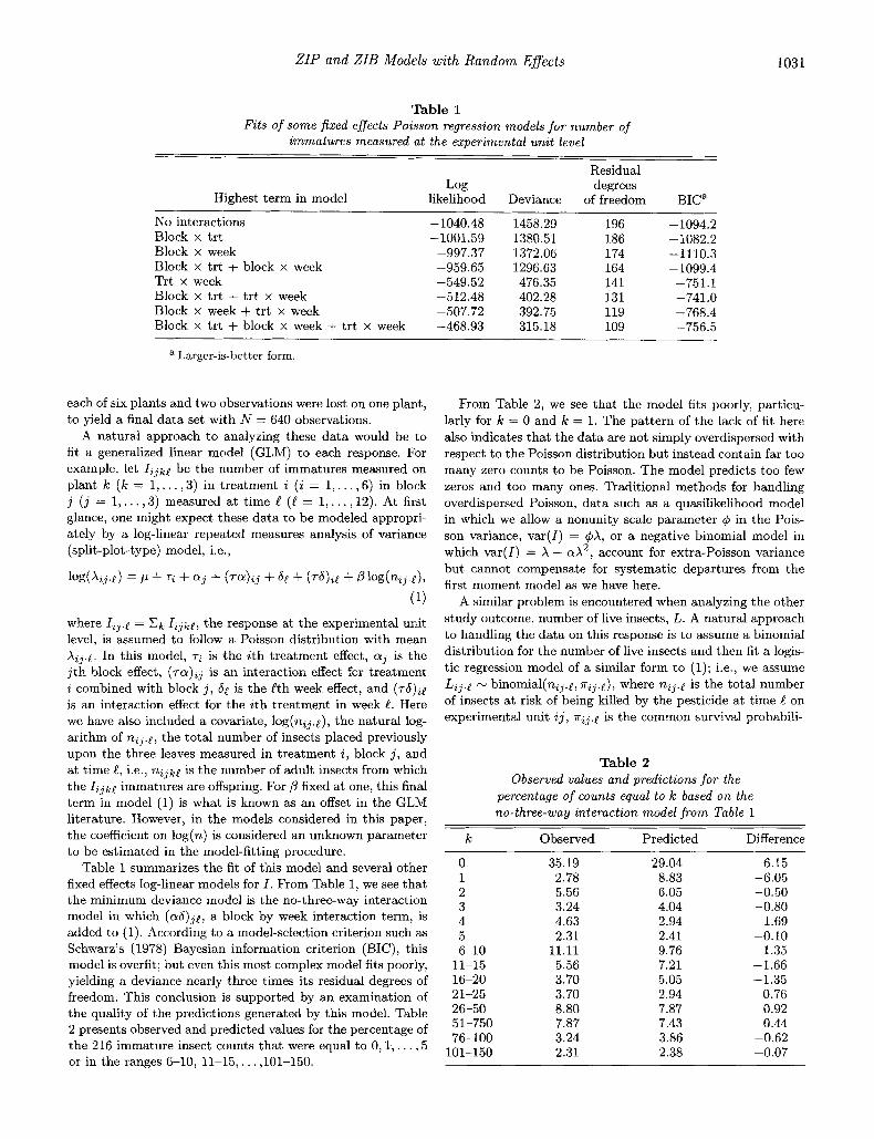
Table 1 Fits of some fixed effects Poisson regression models for number of

immatures measured at the experimental unit level

Highest term in model Log

likelihood Deviance

~~

Residual degrees

of freedom

No interactions Block x t r t Block x week Block x tr t + block x week Trt x week Block x t r t + tr t x week Block x week + tr t x week Block x tr t + block x week + tr t x week

-1040.48 -1001.59 -997.37 -959.65 -549.52 -512.48 -507.72 -468.93

1458.29 1380.51 1372.06 1296.63 476.35 402.28 392.75 315.18

196 186 174 164 141 131 119 109

BICa

-1094.2 -1082.2 -1110.3 -1099.4 -751.1 -741.0 -768.4 -756.5

a Larger-is-better form

each of six plants and two observations were lost on one plant, to yield a final data set with N = 640 observations.

A natural approach to analyzing these data would be to fit a generalized linear model (GLM) to each response. For example, let I i j k e be the number of immatures measured on plant k ( k = 1,. . . ,3) in treatment i (i = 1,. . . ,6) in block j (j = 1,. . . ,3) measured at time l (l = 1,. . . ,12). At first glance, one might expect these data to be modeled appropri- ately by a log-linear repeated measures analysis of variance (split-plot-type) model, i.e.,

where IZ3.e = I i j k e , the response at the experimental unit level, is assumed to follow a Poisson distribution with mean Xi j .e . In this model, ~i is the i th treatment effect, aj is the j t h block effect, (7-a)ij is an interaction effect for treatment i combined with block j , 6e is the l t h week effect, and ( ~ 6 ) i e is an interaction effect for the ith treatment in week l. Here we have also included a covariate, log(nij.e), the natural logarithm of nij.e, the total number of insects placed previously upon the three leaves measured in treatment i , block j , and at time l , i.e., n i j k e is the number of adult insects from which the I i j k e immatures are offspring. For 0 fixed at one, this final term in model (1) is what is known as an offset in the GLM literature. However, in the models considered in this paper, the coefficient on log(n) is considered an unknown parameter to be estimated in the model-fitting procedure.

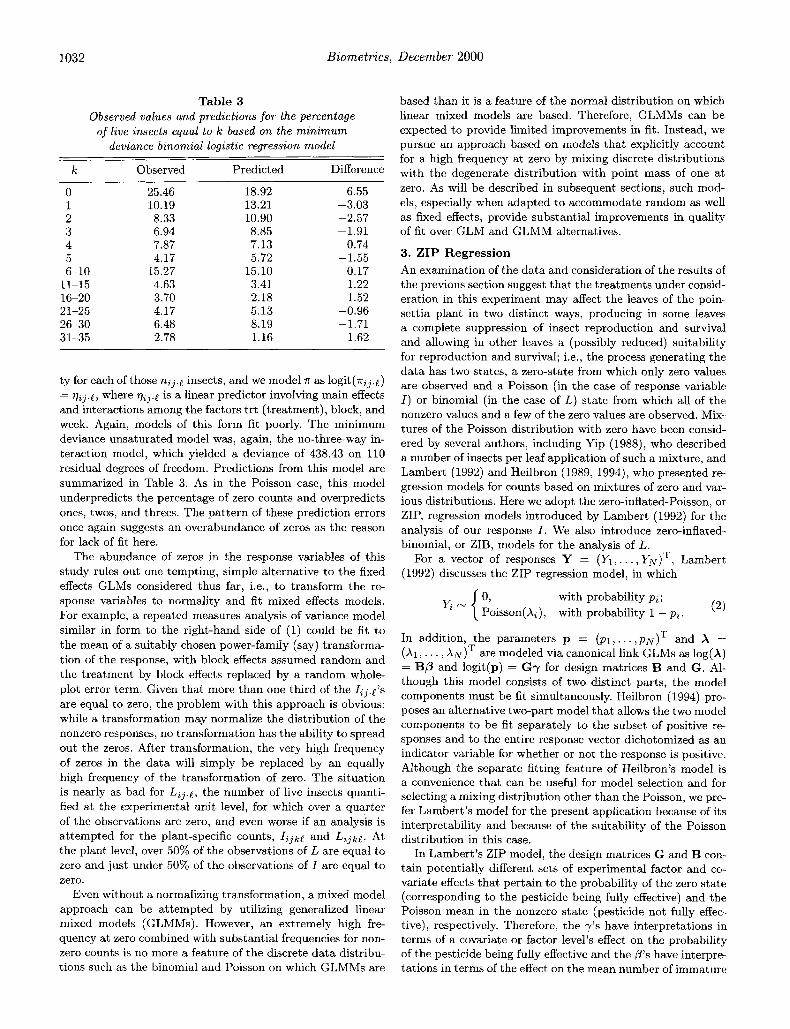
Table 1 summarizes the fit of this model and several other fixed effects log-linear models for I . From Table 1, we see that the minimum deviance model is the no-three-way interaction model in which (a&)je, a block by week interaction term, is added to (1). According to a model-selection criterion such as Schwarz’s (1978) Bayesian information criterion (BIC), this model is overfit; but even this most complex model fits poorly, yielding a deviance nearly three times its residual degrees of freedom. This conclusion is supported by an examination of the quality of the predictions generated by this model. Table 2 presents observed and predicted values for the percentage of the 216 immature insect counts that were equal to 0, I,. . . , 5 or in the ranges 6-10, 11-15,. . . ,101-150.

From Table 2, we see that the model fits poorly, particularly for k = 0 and k = 1. The pattern of the lack of fit here also indicates that the data are not simply overdispersed with respect to the Poisson distribution but instead contain far too many zero counts to be Poisson. The model predicts too few zeros and too many ones. Tkaditional methods for handling overdispersed Poisson, data such as a quasilikelihood model in which we allow a nonunity scale parameter q f J in the Pois- son variance, var(I) = qfJX, or a negative binomial model in which var(I) = X + ax2, account for extra-Poisson variance but cannot compensate for systematic departures from the first moment model as we have here.

A similar problem is encountered when analyzing the other study outcome, number of live insects, L. A natural approach to handling the data on this response is to assume a binomial distribution for the number of live insects and then fit a logistic regression model of a similar form to (1); i.e., we assume L,, e N binomial(n,, e , 7rZ3 e), where n,,.e is the total number of insects at risk of being killed by the pesticide at time l on experimental unit 23, 7rt7 e is the common survival probabili-

Table 2 Observed values and predictions for the

percentage of counts equal to k bused on the no-three-way interaction model from Table 1

k Observed Predicted Difference

0 1 2 3 4 5 6-10

11-15 16-20 21-25 26-50 51-750 76-100

101-150

35.19 2.78 5.56 3.24 4.63 2.31

11.11 5.56 3.70 3.70 8.80 7.87 3.24 2.31

29.04 8.83 6.05 4.04 2.94 2.41 9.76 7.21 5.05 2.94 7.87 7.43 3.86 2.38

6.15 -6.05 -0.50 -0.80

1.69 -0.10

1.35 -1.66 -1.35

0.76 0.92 0.44

-0.62 -0.07

1032 Biometries, December 2000

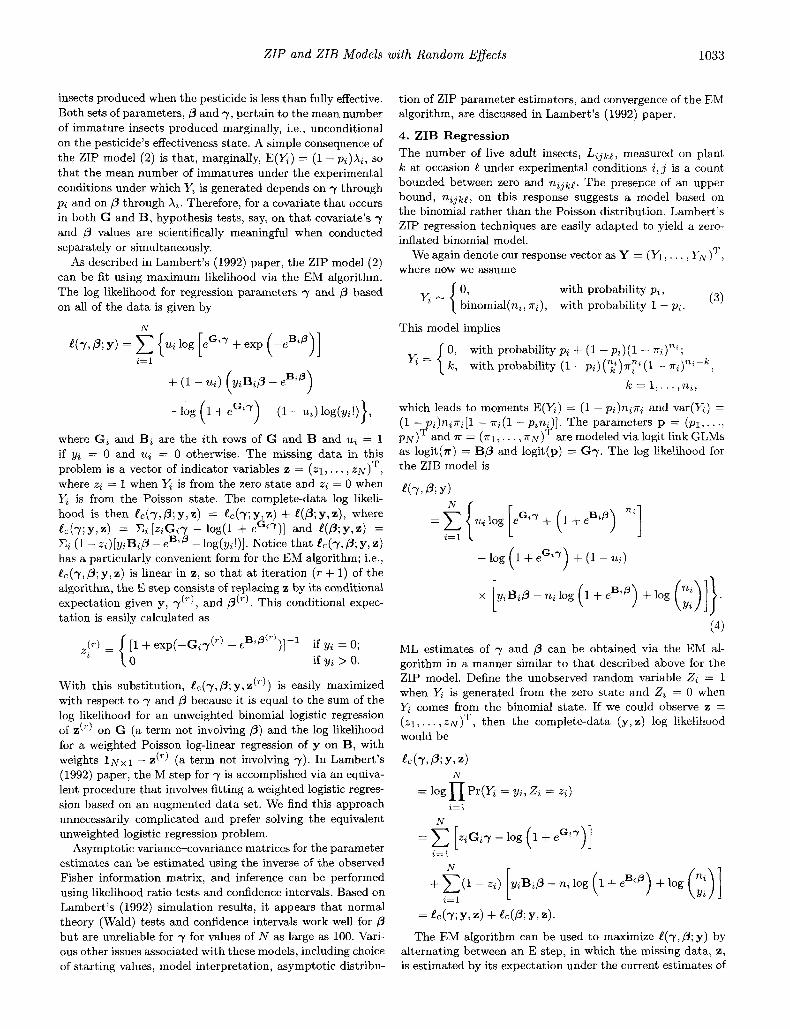
Table 3 Observed values and predictions for the percentage

of live insects equal t o k based o n the minimum deviance binomial logistic regression model

k Observed Predicted Difference

0 1 2 3 4 5 6-10

11-15 16-20 21-25 26-30 31-35

25.46 10.19 8.33 6.94 7.87 4.17

15.27 4.63 3.70 4.17 6.48 2.78

18.92 13.21 10.90 8.85 7.13 5.72

15.10 3.41 2.18 5.13 8.19 1.16

6.55 -3.03 -2.57 -1.91

0.74 -1.55

0.17 1.22 1.52

-0.96 -1.71

1.62

ty for each of those nij.e insects, and we model 7r as logit(7rij.e) = vij.!, where qij.! is a linear predictor involving main effects and interactions among the factors tr t (treatment), block, and week. Again, models of this form fit poorly. The minimum deviance unsaturated model was, again, the no-three-way interaction model, which yielded a deviance of 438.43 on 110 residual degrees of freedom. Predictions from this model are summarized in Table 3. As in the Poisson case, this model underpredicts the percentage of zero counts and overpredicts ones, twos, and threes. The pattern of these prediction errors once again suggests an overabundance of zeros as the reason for lack of fit here.

The abundance of zeros in the response variables of this study rules out one tempting, simple alternative to the fixed effects GLMs considered thus far, i.e., to transform the response variables to normality and fit mixed effects models. For example, a repeated measures analysis of variance model similar in form to the right-hand side of (1) could be fit to the mean of a suitably chosen power-family (say) transformation of the response, with block effects assumed random and the treatment by block effects replaced by a random whole- plot error term. Given that more than one third of the Iij.e’s are equal to zero, the problem with this approach is obvious: while a transformation may normalize the distribution of the nonzero responses, no transformation has the ability to spread out the zeros. After transformation, the very high frequency of zeros in the data will simply be replaced by an equally high frequency of the transformation of zero. The situation is nearly as bad for Lij.e, the number of live insects quanti- fied at the experimental unit level, for which over a quarter of the observations are zero, and even worse if an analysis is attempted for the plant-specific counts, I i j k e and L i j k e . At the plant level, over 50% of the observations of L are equal to zero and just under 50% of the observations of I are equal to zero.

Even without a normalizing transformation, a mixed model approach can be attempted by utilizing generalized linear mixed models (GLMMs). However, an extremely high frequency at zero combined with substantial frequencies for nonzero counts is no more a feature of the discrete data distributions such as the binomial and Poisson on which GLMMs are

based than it is a feature of the normal distribution on which linear mixed models are based. Therefore, GLMMs can be expected to provide limited improvements in fit. Instead, we pursue an approach based on models that explicitly account for a high frequency at zero by mixing discrete distributions with the degenerate distribution with point mass of one at zero. As will be described in subsequent sections, such models, especially when adapted to accommodate random as well as fixed effects, provide substantial improvements in quality of fit over GLM and GLMM alternatives.

3. ZIP Regression An examination of the data and consideration of the results of the previous section suggest that the treatments under consideration in this experiment may affect the leaves of the poinsettia plant in two distinct ways, producing in some leaves a complete suppression of insect reproduction and survival and allowing in other leaves a (possibly reduced) suitability for reproduction and survival; i.e., the process generating the data has two states, a zero-state from which only zero values are observed and a Poisson (in the case of response variable I ) or binomial (in the case of L ) state from which all of the nonzero values and a few of the zero values are observed. Mix- tures of the Poisson distribution with zero have been considered by several authors, including Yip (1988), who described a number of insects per leaf application of such a mixture, and Lambert (1992) and Heilbron (1989, 1994), who presented regression models for counts based on mixtures of zero and various distributions. Here we adopt the zero-inflated-Poisson, or ZIP, regression models introduced by Lambert (1992) for the analysis of our response I . We also introduce zerc-inflated- binomial, or ZIB, models for the analysis of L.

For a vector of responses Y = (E, . . . , YN).’, Lambert (1992) discusses the ZIP regression model, in which

with probability p,; K - { O , Poisson(&), with probability 1 - p,. (2)

In addition, the parameters p = ( P I , . . . , p ~ ) ~ and X = (Xi , . . . , X N ) ~ are modeled via canonical link GLMs as log(X) = BP and logit(p) = Gy for design matrices B and G . Al- though this model consists of two distinct parts, the model components must be fit simultaneously. Heilbron (1994) pro- poses an alternative two-part model that allows the two model components to be fit separately to the subset of positive responses and to the entire response vector dichotomized as an indicator variable for whether or not the response is positive. Although the separate fitting feature of Heilbron’s model is a convenience that can be useful for model selection and for selecting a mixing distribution other than the Poisson, we prefer Lambert’s model for the present application because of its interpretability and because of the suitability of the Poisson distribution in this case.

In Lambert’s ZIP model, the design matrices G and B contain potentially different sets of experimental factor and covariate effects that pertain to the probability of the zero state (corresponding to the pesticide being fully effective) and the Poisson mean in the nonzero state (pesticide not fully effective), respectively. Therefore, the 7’s have interpretations in terms of a covariate or factor level’s effect on the probability of the pesticide being fully effective and the p’s have interpretations in terms of the effect on the mean number of immature

ZIP and ZIB Models with Random Eflects 1033

insects produced when the pesticide is less than fully effective. Both sets of parameters, 0 and y, pertain to the mean number of immature insects produced marginally, i.e., unconditional on the pesticide’s effectiveness state. A simple consequence of the ZIP model (2) is that, marginally, E(Y,) = (1 - p i ) & , so that the mean number of immatures under the experimental conditions under which Yi is generated depends on y through pi and on P through Xi . Therefore, for a covariate that occurs in both G and B, hypothesis tests, say, on that covariate’s y and 0 values are scientifically meaningful when conducted separately or simultaneously.

As described in Lambert’s (1992) paper, the ZIP model (2) can be fit using maximum likelihood via the EM algorithm. The log likelihood for regression parameters y and 0 based on all of the data is given by

N

l(y, P; y) = c { u, log [eGzy + exp ( -eBt’)] 2 = 1

+ (1 - uz) ( Y A I ~ - eBJ)

- log (1 + , c ,y ) - (1 - u,) log(y,!)},

where G, and B, are the zth rows of G and B and u, = 1 if y, = 0 and u, = 0 otherwise. The missing data in this

T problem is a vector of indicator variables z = (q, . . . , z ~ ) , where z, = 1 when Y, is from the zero state and z, = 0 when Y, is from the Poisson state. The complete-data log likelihood is then &(y, 0; y, z) = &(y; y, z) + [(p; y, z), where Cc(y;y,z) = C, [zZG2y - log(1 + eGtY)] and l(O;y,z) = C, (1 - z,)[y,B,P - eBtP - log(y,!)]. Notice that &(y,P; y, z) has a particularly convenient form for the EM algorithm; i.e., &(y, 0; y, z) is linear in z, so that at iteration ( r + 1) of the algorithm, the E step consists of replacing z by its conditional expectation given y, and P(’). This conditional expectation is easily calculated as

- [l + exp(-G,y(T) - eBtpP‘”)]-l if y, = 0; if y, > 0. z2 -{o

With this substitution, &(y, 0; y, ~ ( ~ 1 ) is easily maximized with respect to y and 0 because it is equal to the sum of the log likelihood for an unweighted binomial logistic regression of dT) on G (a term not involving 0) and the log likelihood for a weighted Poisson log-linear regression of y on B, with weights 1 ~ ~ 1 - z ( ~ ) (a term not involving y). In Lambert’s (1992) paper, the M step for y is accomplished via an equivalent procedure that involves fitting a weighted logistic regression based on an augmented data set. We find this approach unnecessarily complicated and prefer solving the equivalent unweighted logistic regression problem.

Asymptotic variance-covariance matrices for the parameter estimates can be estimated using the inverse of the observed Fisher information matrix, and inference can be performed using likelihood ratio tests and confidence intervals. Based on Lambert’s (1992) simulation results, it appears that normal theory (Wald) tests and confidence intervals work well for but are unreliable for y for values of N as large as 100. Vari- ous other issues associated with these models, including choice of starting values, model interpretation, asymptotic distribu-

tion of ZIP parameter estimators, and convergence of the EM algorithm, are discussed in Lambert’s (1992) paper.

4. ZIB Regression The number of live adult insects, L i j k g , measured on plant k at occasion l under experimental conditions i , j is a count bounded between zero and n i j k g . The presence of an upper bound, n i j k e , on this response suggests a model based on the binomial rather than the Poisson distribution. Lambert’s ZIP regression techniques are easily adapted to yield a zero- inflated binomial model.

We again denote our response vector as Y = (Yl , . . . , Y,)T, where now we assume

(3) K - { O . with probability pi,

binomial(ni, ri), with probability 1 - pi.

This model implies

0, k ,

with probability pi + (1 - pi)( l - ~ i ) ~ ~ ;

with probability (1 - pi) f i)r:% (1 -

k = 1,. . . ,ni, { y ,=

which leads to moments E(Yi) = (1 - p i ) n i ~ i and var(x) = (1 - p i ) n g i [ l - ~ i ( l -pin;)] . The parameters p = ( P I , . . ., p ~ ) ~ and 7 = (T I , . . . , T N ) are modeled via logit link GLMs as logit(w) = BP and logit(p) = Gy. The log likelihood for the ZIB model is

e(Y, P; Y)

(4)

ML estimates of y and 0 can be obtained via the EM algorithm in a manner similar to that described above for the ZIP model. Define the unobserved random variable 2, = 1 when Y, is generated from the zero state and 2, = 0 when Y , comes from the binomial state. If we could observe z = ( z l , . . . , z ~ ) ~ , then the complete-data (y, z) log likelihood would be

l c ( Y , P; Y ? 2)

= log N

Pr(K = y,, Z, = z,) a = 1

hi

= [ziGiy - log (1 + eGi7 ) ] i=l

= &(Y;Ylz) +lc(P;y,z).

The EM algorithm can be used to maximize l ( y , P; y) by alternating between an E step, in which the missing data, 8,

is estimated by its expectation under the current estimates of

1034 Biometrics, December 2000

(y,p), and a maximization step, in which &(y,P) evaluated at the current (fixed) estimate of z is maximized with respect to both y and p. As in the ZIP regression model, this procedure is particularly convenient because &(y, p; y, z) is linear in z and also splits into a sum of two exponential family (in this case, binomial) log likelihoods, each of which depends on only one of the regression parameters y and p.

In more detail, the EM algorithm begins with starting values (y('), p(O)) and proceeds iteratively. At iteration T + 1, we have the following three steps:

(1) E step. Estimate 2, by its conditional mean ZZ(.) =

E(Zi I yi, y(.),p(')) under current estimates of the regression parameters. This expectation is given by

z;) = Pr zero state 1 yi, -+'I, ,(.)) ( = Pr(yi I zero state) Pr(zero state)

t [ Pr(yi 1 zero state) Pr(zero state)

1 + Pr(yi 1 binomial) Pr(binomia1)

if yz > 0.

(2) M step for y. Find y(T+l) by maximizing &(y; y, Z")). This can be accomplished by performing an unweighted binomial logistic regression of Z(') on design matrix G using a binomial denominator of one for each observation.

(3) M step for p. Find p(T+l) by maximizing &(P; y, Z")) = C, (1 - Z,'")[y,B,P - nz log(1 + e B t P ) + log (;:)I. This can be done via a weighted logistic regression with weights (1 - Z,'.)), i = 1, . . . , N , and binomial error distribution with denominators n1, . . . , nN.

Good starting values for p in the EM algorithm can be obtained by maximizing the positive part binomial log likelihood as

a+@; Y+)

-1% [l- ( l + P y i ] +log(;;)}.

As in the ZIP model, the starting value chosen for y has been less important in our experience. Following Lambert (1992), we suggest an initial value for the intercept in y equal to the observed average probability of an excess zero, or $0 = [#(yi = 0) - EL_, (1 - T ~ ) ~ ~ ] / N , and an initial value of zero for the remaining elements of y.

Convergence of the EM algorithm in this problem follows from arguments similar to those given by Lambert (1992, Ap- pendix A.l). Alternative algorithms, such as Newton-Raph- son or Newton-Raphson with Fisher scoring, for maximizing the log likelihood (equation (4)) can be used in this problem. However, the EM algorithm is simpler to program, especially if GLM fitting routines are available. In addition, the EM algorithm and its extensions (e.g., Monte Carlo EM; McCul- loch, 1997) have been useful for fitting models with random effects, and we make such use of the algorithm in Section 5. Our experience regarding the convergence of the EM and Newton-Raphson algorithms for fitting the zero-inflated models discussed in this paper is in agreement with Lambert's summarizing statement that "In short, the ZIP . . . regressions were not difficult to fit" (Lambert, 1992, p. 6).

5. ZIP and ZIB Regression with Random Effects The best ZIP and ZIB models that we fit to the whitefly data model the data much more closely than corresponding generalized linear models (as in Section 2). For example, based on BIC, the best fitting ZIB model that we fit to the number of live insects response was

logit@) = p + tr t + block +week

and

logit(7r) = p + tr t + block + week + tr t x block + tr t x week.

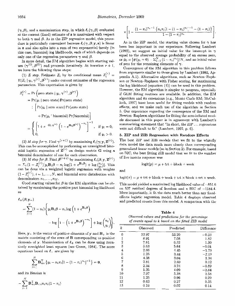
This model yielded a maximized log likelihood value of -851.6 on 537 residual degrees of freedom and a BIC of -1184.4. More importantly, it fit the data much better than any fixed- effects logistic regression model. Table 4 displays observed and predicted counts from this model. A comparison with the

Table 4 Observed values and predictions for the percentage of counts equal to k based on the fitted ZIB model

k 0 bserved Predicted Difference Here, y+ is the vector of positive elements of y and B+ is the matrix consisting of the rows of B corresponding to positive elements of y. Maximization of !+ can be done using iteratively reweighted least squares (see Green, 1984). The score equations based on e+ are given by

N

i=l

and its Hessian is N

0 1 2 3 4 5 6 7 8 9

10 11 12 13

52.97 8.91 7.81 5.63 2.66 1.25 4.38 2.81 2.34 1.25 7.97 1.25 0.63 0.16

53.20 7.08 6.52 5.64 4.45 3.44 3.04 2.69 3.24 4.09 5.38 0.96 0.27 0.02

-0.23 1.82 1.30

-0.01 -1.79 -2.19

1.34 0.12

-0.89 -2.84

2.58 0.29 0.35 0.14

i=l

ZIP and ZIB Models with Random Eflects 1035

results of Table 3 reveals a substantial improvement when we allow a mixture of the binomial distribution with zero.

However, these fixed effects models are based on the assumption of independence among the responses. In a repeated measures design such as that of the whitefly data, such an assumption is clearly violated. While there may be independence from plant to plant, there almost certainly is correlation among repeated observations on the same plant. Neither the ZIP nor ZIB models make allowances for this dependence, nor do they separate plant-to-plant heterogeneity from the residual variance (at the experimental unit level) remaining after accounting for design factors. Such inadequacies in the model can seriously affect the validity of statistical inference.

Recently, many researchers have incorporated random effects into a wide variety of regression models to account for correlated responses and multiple sources of variance. We pro- pose this approach in the zero-inflated Poisson and binomial models discussed earlier in the paper. In particular, we consider models in which a random intercept is added to the exponential family portion of the model.

5.1 ZIP Regression with a Random Intercept Suppose our response vector Y contains data from K independent clusters so that Y = (YT,. . . ,Y:)T, where Yi =

(61,. . . , % T , ) ~ . We assume that, conditional on a random effect bi,

with probability p i j ; with probability (1 - p i j ) , ' 3 { Poisson(Aij), O,

where we model Xi = ( A i l , . . . , A ~ T , ) ~ and pi = (pi1 , . . . , p , ~ , ) ~ with log-linear and logistic regression models

log(&) = BiP +obi and

logit(pi) = Giy, i = 1,. . . ,K .

Here, B = (BT , . . . , BZ)T and G = (GT , . . . , GZ)T are design matrices, and we assume bl , . . . , bK are independent standard normal random variables.

Let + = (yT,PT,a)T be the combined parameter vector. The log likelihood for the ZIP model with random intercept is

L"

where

uZ3 [exp(G,,y) + exp (-eBtJPtob'

Here, 4 denotes the standard normal probability density function, and uZJ = 1 if yZJ = 0 and ut3 = 0 otherwise.

Maximization of (5) with respect to + is complicated by the integration with respect to b,. Several authors (e.g., Hinde, 1982; Anderson and Aitkin, 1985) have dealt with the same challenge in the context of a GLM with random intercept by employing the EM algorithm with Gaussian quadrature. This is a natural approach to employ here because we are already using the EM algorithm in the fixed effects version of the model. By regarding both the state of the process (zero state versus Poisson state) and the random effects as missing data, we can use the EM algorithm to more conveniently maximize

Let ZZ3 = 1 when y Z 3 comes from the zero state and Zt3 = 0 when Yz3 comes from the Poisson(AtJ) state. The complete- data log likelihood is

(5).

u+; Y, z, b)

= log f(b; +) + 1% f ( Y , z I b; +) K

i=l

i=l j=1 '

The ( r + 1)th iteration of the EM algorithm consists of the following three steps:

(1) E step. The E step requires the calculation of Q(+ I +(')) = E(1og f(y, z, b; +) I y, + ( T ) ) , where here the expectation is with respect to the joint distribution of z, b given y and +('I, the parameter estimate based on the r th iteration. This expectation can be taken in two steps,

Q (+ I + ( r ) )

The inner expectation is with respect to z only and, since log f (y , z, b 1 +) is linear with respect to z, this expectation becomes log f (y , Z('), b 1 +), where Z ( T ) contains elements

Note that Z$) depends on bi , so we will emphasize this

dependence by writing Z$)(bi). To complete the E step, we now need to take the expectation with respect to the distribution of b I y, Dropping terms that don't involve + and are therefore irrelevant in the M step, it follows that

1036 Biornetrics, December 2000

Here we have used the fact that

Using rn-point Gaussian quadrature to approximate these integrals, we have

Q (+ I +('I)

x f (Yz; +'" I be) we

EL [1 - z $ ) ( b e ) ]

CE1 f ( ~ i ; I be)we + x [ ~ i j ( B i j P $. a b e ) - exp(BijP + .be)]

x f(yi;+(') I be)we , 1 where be are quadrature points and we the associated weights.

(2) M step f o r y. Notice that, as in the EM algorithm for the fixed effects ZIP model, Q(+ I + ( r ) ) decomposes into the sum of a term involving only y and a second term involving only /3. Therefore, we maximize Q(+ I +('I) with respect to y by maximizing the first term. This maximization can be done via a weighted logistic regression of Z k ' ( b e ) , i = 1,. . . , K , j = 1 , . . . ,Ti, t = 1,. . . , rn, on G 8 lmx l with weights f(yi;+(') I bg)wt /g j" , where gjT' = C& f ( y i ; + ( ' ) I be)we, i.e., we perform a weighted logistic regression with an ~ r n x I response vector (2;;) ( b l ) , . . . ,z!;) (bm) , z;;' ( b l ) , . . . , Zi;'(bm), . . . , Z$iK (bn l ) )T , a rnatrix of explanatory variables equal to the matrix obtained by repeating each row of G rn times, and weight

23

f ( y i ; +"' I be)We/gjT' = [ ~ T A ~ f (y i j ; I be)lwe/gj"

(constant over index j ) corresponding to the (i , j ,e)th response.

(3) M step f o r p , 0. Maximization of the second term in Q(+ 1 +(T)) with respect to P and o can be done simultaneously. Define B' = [(B 8 lm), ( 1 ~ 8 ( b l , . . . , b m ) T ) ] , P* = (/3T,o)T. Maximization with respect to /3* can be

accomplished by fitting a weighted log-linear regression of y 8 lmx l on B* with weights

[I- z j i ) ( b e ) ~ f ( ~ z ; +"' I be)we/g j ' ) ,

i = 1,. . . , K , j = 1,. . . ,T,, e = 1,. . . ,rn. 5.2 ZIB Regression with a Random Intercept In the ZIB regression model with random intercept, we assume that, conditional on a random effect bi,

with probability p i j ; with probability (1 - p i j ) , { binomial(nij, O , nsj),

Yij N

where we model 7ri = (7ri1,. . . , T ~ T ? ) ~ and pi using logistic regression models

logit(7ri) = BiP + obi

logit(pi) = Giy,

and i = 1,. . . ,K .

Again, we assume bl , . . . , bK are independent standard normal random variables. The log likelihood for this model is as in ( 5 ) but now where

Pr (Kj = yij I bi) = [pij + (1 - P i j ) ( l - 7 4 n , q u , 3

As in the ZIP mixed model, the complete-data log likelihood can be constructed for use in the EM algorithm as

fd+; Y, 2, b)

+log (;::)I}. The ( r + l ) t h iteration of the EM algorithm consists of the following three steps:

ZIP and ZIB Models with Random EfSects 1037

(1) E step. In the E step, Q(+ 1 +('I) = E[logf(y, Z('), b 1 + ) I , where Z(?) contains elements

Zt3 (7.) (b,) = { i; Taking the expectation with respect to the distribution of b 1 y, +('I and dropping irrelevant terms, we obtain

which, using Gaussian quadrature, is approximately equal to

(2) M step for y. Maximization of &(+ I +('I) with respect to y can be done exactly as in Section 5.1.

(3) A4 step for P, u. Maximization of &(+ 1 +('I) with respect to /3* can be accomplished by fitting a weighted logistic regression of y @ l m x l on B* with weights [l - ~ $ ) ( b ~ ) l j ( y ~ ; + ( ~ ) 1 be)wp/gjT), i = I , . . . ,x , j = I , . . . ,T,, e = 1 , . . . ,m, and binomial denominators (1211,. . . , 7 ~ 1 ~ ~ , 7~21,

In both the ZIP mixed and ZIB mixed models, an estimate of the asymptotic variance-covariance matrix of the MLE 9 can be obtained by inverting the observed Fisher information matrix evaluated at +. For the models fit in this paper, this information matrix was obtained numerically. Based on Lambert's (1992) results, Wald tests and confidence intervals based on the asymptotic normality of 9 may perform poorly in ZIP mixed and ZIB mixed models unless the sample size is quite large. Instead, we follow Lambert (1992) in recommend-

. . . , ~ K T K ) ~ @ 1 ~ ~ x 1 .

ing likelihood ratio tests and confidence intervals as the basis of inference when N is moderate to small. 6. Examples 6.1 Whitefly Data Based on the experimental design, a reasonable starting point for selecting a ZIP mixed model for the number of immature insects per leaf data is to adapt the repeated measures analysis of variance model given in equation (1). Informally, we write the model for the Poisson-state mean as

log(X) = p + plant + block + trt + week + trt x block + trt x week + log(n), (6)

where p is a fixed intercept, plant is a random plant-specific effect, log(n) represents a covariate corresponding to the natural logarithm of the number of adult insects placed on the leaf prior to measurement of the response, and the other terms are fixed effects corresponding to factors and two-way interactions among the factors. We fit several models in which the relationship given in (6) is assumed combined with various choices for the linear predictor associated with logit(p). Based on BIC, we selected the model with the covariate log(n) plus all main effects in the linear predictor for logit(p). This model yielded a maximum log likelihood of -1219.3 and a BIC of -1561.8 on 534 residual degrees of freedom.

For comparison, we fit the ZIP model with the same design matrices B and G but no random effects. This model yielded a maximum log likelihood value of -1238.4 on 535 residual degrees of freedom. Notice that inclusion of a random plant effect has resulted in a significantly improved fit. Under Ho: u = 0, two times the difference in the maximum log likelihood values for the ZIP and ZIP mixed versions of the model has an asymptotic distribution which is a 50:50 mixture of ~ ' ( 0 ) and ~ ~ ( 1 ) . Noting that Ho places the identifiable parameter u2 on the boundary of its parameter space, this result follows from the work of Stram and Lee (1994) and authors referenced therein. Thus an approximate p-value for Ho is ( 1 / 2 ) P r [ ~ ~ ( l ) > 38.21 < .0001.

As mentioned in Section 2, an alternative class of models worthy of consideration for these data is the class of GLMMs. Lambert (1992) compared her ZIP regression model with a Poisson-gamma (negative binomial) GLMM and demonstrated the superiority of her approach for the data set that she analyzed in that paper. We consider a similar Poisson-gamma model for response variable I in the whitefly data set. In this model, it is assumed that counts from different weeks j on the same plant i are Poisson(XijRi), where Ri is assumed to follow a gamma(cu,a) distribution and log(Xij) = XijP. We also explored a Poisson-normal model of the same form except we assumed Ri - N(0,u:). Restricting attention to identifiable models in these classes, the best fitting Poisson-gamma and Poisson-normal models that we were able to fit to the whitefly data were of the form given in (6), although certain of the design matrix columns corresponding to two-way interaction effects were eliminated in each case for identifiability.

These models fit better than the corresponding Poisson models (e.g., the negative binomial model gave a maximum log likelihood of -1583.1 versus -1650.8 for the Poisson model). However, they do not fit nearly as well as the ZIP and ZIP mixed models described above. In Figure 1 (cf., Lambert,

Biornetrics, December 2000

"'1 0 03

B

8

(2000). Results based on ZIP mixed and ZIB mixed models are qualitatively the same. Briefly, for I , contrasts between

0 Negative binomial the control treatment and all active treatments and between A ZIP-mixed the standard active treatment (H) and the subirrigation

treatments (0, 1, 2,4) were highly significant when performed on and y or on ,L3 and y simultaneously. All effects were in the expected direction, with active treatments suppressing

Poisson-normal ;I,i I

+ 8 whitefly reproduction, most effectively when subirrigation was used to deliver the pesticide. A significant disorderly

4 L\

B 9 A 0

4 interaction between week and the subirrigation treatments prevented a marginal comparison between the 0, 1, 2, and 4 treatments, but the treatment by week profile plot of the marginal mean number of immatures suggested a trend

h 0 6

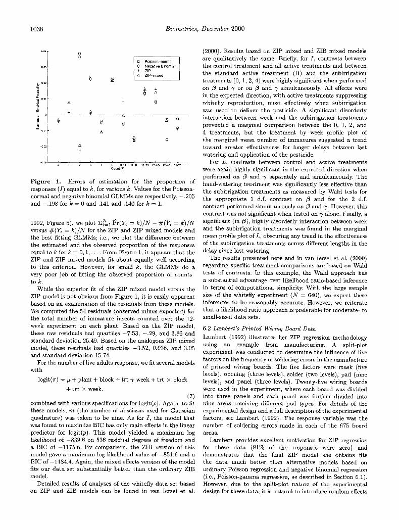
Figure 1. Errors of estimation for the proportion of responses ( I ) equal to k , for various k . Values for the Poisson- normal and negative binomial GLMMs are respectively, -.205 and -.198 for k = 0 and ,141 and ,140 for k = 1.

1992, Figure 5), we plot E L l Pr(Y, = k ) / N - # ( y Z = k ) / N versus #(Yi = k ) / N for the ZIP and ZIP mixed models and the best fitting GLMMs; i.e., we plot the difference between the estimated and the observed proportion of the responses equal to k for k = 0,1, . . . . From Figure 1, it appears that the ZIP and ZIP mixed models fit about equally well according to this criterion. However, for small k , the GLMMs do a very poor job of fitting the observed proportion of counts to k .

While the superior fit of the ZIP mixed model versus the ZIP model is not obvious from Figure 1, it is easily apparent based on an examination of the residuals from these models. We computed the 54 residuals (observed minus expected) for the total number of immature insects counted over the 12- week experiment on each plant. Based on the ZIP model, these raw residuals had quartiles -7.53, -.29, and 3.86 and standard deviation 25.49. Based on the analogous ZIP mixed model, these residuals had quartiles -3.52, 0.036, and 3.05 and standard deviation 15.74.

For the number of live adults response, we fit several models with

logit(r) = p + plant + block + trt + week + tr t x block + trt x week,

(7) combined with various specifications for logit(p). Again, to fit these models, m (the number of abscissas used for Gaussian quadrature) was taken to be nine. As for I , the model that was found to maximize BIC has only main effects in the linear predictor for logit(p). This model yielded a maximum log likelihood of -839.6 on 536 residual degrees of freedom and a BIC of -1175.6. By comparison, the ZIB version of this model gave a maximum log likelihood value of -851.6 and a BIC of -1184.4. Again, the mixed effects version of the model fits our data set substantially better than the ordinary ZIB model.

Detailed results of analyses of the whitefly data set based on ZIP and ZIB models can be found in van Iersel et al.

toward greater effectiveness for longer delays between last watering and application of the pesticide.

For L, contrasts between control and active treatments were again highly significant in the expected direction when performed on p and y separately and simultaneously. The hand-watering treatment was significantly less effective than the subirrigation treatments as measured by Wald tests for the appropriate 1 d.f. contrast on ,L3 and for the 2 d.f. contrast performed simultaneously on p and y. However, this contrast was not significant when tested on y alone. Finally, a significant (in p), highly disorderly interaction between week and the subirrigation treatments was found in the marginal mean profile plot of L, obscuring any trend in the effectiveness of the subirrigation treatments across different lengths in the delay since last watering.

The results presented here and in van Iersel et al. (2000) regarding specific treatment comparisons are based on Wald tests of contrasts. In this example, the Wald approach has a substantial advantage over likelihood ratio-based inference in terms of computational simplicity. With the large sample size of the whitefly experiment ( N = 640), we expect these inferences to be reasonably accurate. However, we reiterate that a likelihood ratio approach is preferable for moderate- to small-sized data sets.

6.2 Lambert's Printed Wiring Board Data Lambert (1992) illustrates her ZIP regression methodology using an example from manufacturing. A split-plot experiment was conducted to determine the influence of five factors on the frequency of soldering errors in the manufacture of printed wiring boards. The five factors were mask (five levels), opening (three levels), solder (two levels), pad (nine levels), and panel (three levels). Twenty-five wiring boards were used in the experiment, where each board was divided into three panels and each panel was further divided into nine areas receiving different pad types. For details of the experimental design and a full description of the experimental factors, see Lambert (1992). The response variable was the number of soldering errors made in each of the 675 board areas.

Lambert provides excellent motivation for ZIP regression for these data (81% of the responses were zero) and demonstrates that the final ZIP model she obtains fits the data much better than alternative models based on ordinary Poisson regression and negative binomial regression (i.e., Poisson-gamma regression, as described in Section 6.1). However, due to the split-plot nature of the experimental design for these data, it is natural to introduce random effects

ZIP and ZIB Models with Random Effects 1039

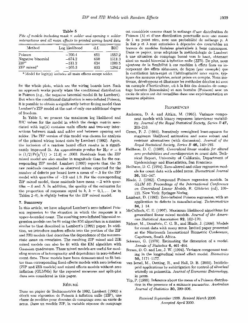
Table 5 Fits of models including mask x solder and opening x solder interactions and all m a i n eflects t o printed wiring board data

Method Log likelihood d.f. BIC

Poisson -700.4 65 1 1557.2 Negative binomial -674.2 650 1511.3 ZIP” -511.2 634 1289.5 ZIP mixed” -505.3 633 1284.2

” Model for logit(p) includes all main effects except solder.

for the whole plots, which are the wiring boards here. Such an approach works poorly when the conditional distribution is Poisson (e.g., the negative binomial model fit by Lambert). But when the conditional distribution is zero-inflated Poisson, it is possible to obtain a significantly better fitting model than Lambert’s ZIP model at the cost of only one additional degree of freedom.

In Table 5, we present the maximum log likelihood and BIG values for the model in which the design matrix associated with log(A) contains main effects and two-way interactions between mask and solder and between opening and solder. The ZIP version of this model was chosen for analysis of the printed wiring board data by Lambert (1992). Again, the inclusion of a random board effect results in a significantly improved fit. An approximate p-value for Ho: (T = 0 is (1/2)Pr[x2(1) > 11.81 = ,0003. Residuals from the ZIP mixed model are also smaller in magnitude than for the corresponding ZIP model. Lambert (1992) reports that the 25 raw residuals computed as observed minus expected for the number of defects per board have a mean of - .3 for the ZIP model with quartiles of -2.9 and 1.9. For the corresponding ZIP mixed model, these residuals have mean -.2 with quartiles -.6 and .5. In addition, the quality of the estimates for the proportion of responses equal to k , lc = O , l , . . . (as in Tables 2-4), is slightly better for the ZIP mixed model.

7. Summary In this article, we have adapted Lambert’s zero-inflated Pois- son regression to the situation in which the response is a upper-bounded count. The resulting zero-inflated binomial regression models can be fit using the EM algorithm in a manner similar to that described in Lambert’s (1992) paper. In addition, we introduce random effects into the portion of the ZIP and ZIB models that describes the dependence of the nonzero- state mean on covariates. The resulting ZIP mixed and ZIB mixed models can also be fit with the EM algorithm with Gaussian quadrature. These mixed models are useful for mod- eling sources of heterogeneity and dependence in zero-inflated count data. These models have been demonstrated to fit better than corresponding fixed-effects models with zero inflation (ZIP and ZIB models) and mixed effects models without zero inflation (GLMMs) for the repeated measures and split-plot data sets considered in this paper.

RBSUME

Dans un papier de Technometrics de 1992, Lambert (1992) a dkcrit une regression de Poisson k inflation nulle (ZIP), une classe de modkles Dour donnkes de comDtaEe avec un excks de

est considkree comme &ant le mBlange d’unc distribution de Poisson (A) et d’une distribution ponctuelle avec une masse de 1 au point zkro, avec une probabilite de mklange p. A la fois p et X sont autoriskes B dkpendre des covariables au travers de modkles linkaires gknkralisks B liens canoniques. Dans ce papier, nous adoptons la mkthodologie de Lambert B une situation de comptage born6 vers le haut, obtenant ainsi un model binomial B inflation nulle (ZIB). De plus, nous ajoutons de la flexibilitk B ces modkles 8, effets fixes en in- corporant des effets alkatoires, de faqon (par exemple) que la corrklation intraisujet et l’hktkrogknkitk inter sujets, typ- iques des mesures rkpktkes, soient prises en compte. Nous mo- tivons, dkveloppons et illustrons les mkthodes dkcrites ici avec un exemple d’horticulture, oii k la fois des donnkes de comptage bornkes (binomiales) et non bornkes (Poisson) avec un excks de zeros ont Btk recueillies dans une experimentation en mesures rkpktkes.

REFERENCES Anderson, D. A. and Aitkin, M. (1985). Variance compo-

nent models with binary responses: interviewer variabil- ity. Journal of the Royal Statistical Society, Series B 47,

Green, P. J. (1984). Iteratively reweighted least-squares for maximum likelihood estimation and some robust and resistant alternatives (with discussion). Journal of the Royal Statistical Society, Series B 46, 149-192.

Heilbron, D. C. (1989). Generalized linear models for altered zero probabilities and overdispersion in count data. Tech- nical Report, University of California, Department of Epidemiology and Biostatistics, San Francisco.

Heilbron, D. C. (1994). Zero-altered and other regression models for count data with added zeros. Biometrical Journal

Hinde, J. (1982). Compound Poisson regression models. In G L I M 82: Proceedings of the International Conference o n Generalised Linear Models, R. Gilchrist (ed), 109- 121. New York: Springer-Verlag.

Lambert, D. (1992). Zero-inflated Poisson regression, with an application to defects in manufacturing. Technometrics

McCulloch, C. E. (1997). Maximum likelihood algorithms for generalized linear mixed models. Journal of the Ameri- can Statistical Association 92, 162-170.

Ridout, M., Demktrio, C. G. B., and Hinde, J. (1998). Models for count data with many zeros. Invited paper presented at the Nineteenth International Biometric Conference, Capetown, South Africa.

Schwarz, G. (1978). Estimating the dimension of a model. Annals of Statistics 6, 461-464.

Stram, D. 0. and Lee, J. W. (1994). Variance component test- ing in the longitudinal mixed effect model. Biometrics

van Iersel, M., Oetting, R., and Hall, D. B. (2000). Imidiclo- prid applications by subirrigation for control of silverleaf whitefly on poinsettia. Journal of Economic Entomology, in press.

Yip, P. (1988). Inference about the mean of a Poisson distribution in the presence of a nuisance parameter. Australian Journal of Statistics 30, 299-306.

203-210.

36, 531-547.

34, 1-14.

50, 1171-1177.

Received September 1999. Revised March 2000. Acceoted April 2000.

- - zeros. Dans un modkle ZIP, la variable rkponse de comptage

Documents

Zero-Inflated Poisson and Binomial Regression with Random Effects