Your Gain Is My Pain: Negative Psychological Externalities ofCash Transfers∗

Johannes Haushofer†, James Reisinger‡, and Jeremy Shapiro§

October 31, 2015

Abstract

We use a randomized controlled trial of unconditional cash transfers in Kenya to study theeffects of exogenous changes in the wealth of neighbors on psychological wellbeing, consumption,and assets. We find that increases in neighbors’ wealth strongly decrease life satisfaction andmoderately decrease consumption and asset holdings. The decrease in life satisfaction inducedby transfers to neighbors more than offsets the direct positive effect of transfers, and is largestfor individuals who did not receive a direct transfer themselves. We find evidence of hedonicadaptation, in that the negative spillover effect of transfers to neighbors decreases over time, ata rate similar to that of direct transfers.

JEL Codes: C93, I14, I31, O12

∗We are grateful to the study participants for generously giving their time. We thank Faizan Diwan, ConorHughes, Chaning Jang, and Kenneth Okumu for excellent research assistance; the team of GiveDirectly (MichaelFaye, Raphael Gitau, Piali Mukhopadhyay, Paul Niehaus, Joy Sun, Carolina Toth, Rohit Wanchoo) for fruitfulcollaboration; and Victoria Baranov, Alexis Grigorieff, Chaning Jang, Michala Iben Riis-Vestergaard, Chris Roth,Janet Currie, Dan Sacks, Tom Vogl, and Ilyana Kuziemko for comments and discussion. All errors are our own. Thisresearch was supported by NIH Grant R01AG039297 and Cogito Foundation Grant R-116/10 to Johannes Haushofer.†Peretsman Scully Hall 427, Princeton University, Princeton, NJ 08544, and Busara Center for Behavioral Eco-

nomics, Nairobi, Kenya. haushofer@princeton.edu‡Peretsman Scully Hall 407, Princeton University, Princeton, NJ 08544, and Busara Center for Behavioral Eco-

nomics, Nairobi, Kenya. reisinger@princeton.edu§Busara Center for Behavioral Economics, Nairobi, Kenya. jeremypshapiro@gmail.com

1

1 Introduction

The idea that relative income affects consumption and welfare has a long tradition in economics.1

Thorstein Veblen famously argued that increases in neighbors’ consumption could lead to increasesin own consumption (Veblen 1899). Similarly, Duesenberry (1949) argues that individual utility isnegatively affected by the income and consumption of others; this claim is known as the RelativeIncome Hypothesis. This paper presents an empirical test of this latter hypothesis.

Empirically, it has been difficult to document a negative effect of the income of others on own well-being, and in particular, to establish causality. Even in the correlational domain, the evidence iscontradictory: the early work of Easterlin suggested that the correlation between income and hap-piness was high within countries, but low across countries (Easterlin 1974; Easterlin 1995; Easterlin2001), raising the possibility that relative considerations, with compatriots as the reference group,matter for happiness. However, apart from the fact that the correlational nature of the data limitsthe interpretability of this analysis, recent work by Stevenson & Wolfers has demonstrated that acorrelation exists even across countries (Stevenson and Wolfers 2008; Sacks, Stevenson, and Wolfers2012). Others have reported similar findings using panel data from Europe (Ferrer-i Carbonell2005; Veenhoven 1984; Stadt, Kapteyn, and Geer 1985; Senik 2004; Clark and Oswald 1996), theUS . Other observational studies on the relationship between income and self-reported wellbeingare similarly inconclusive. Using US panel data, Blanchflower and Oswald (2004) find a negativebut insignificant effect of per capita state income on happiness. McBride (2001) also finds weakevidence of a relative income effect on self-reported happiness. Tomes (1986) find conflicting resultsusing Canadian data on income and self-reported wellbeing, with negative effects of relative incomeon wellbeing on some scales but not others, and different effects for men and women. Luttmer(2005), using data from the National Survey of Families and Households (NSFH), shows that earn-ings increases of neighbors negatively affect individuals’ self-reported happiness. To deal with biasfrom local omitted variables, Luttmer uses predicted local earnings based on the local industry xoccupation composition and national industry x occupation earnings trends. This leaves open thepossibility that unobserved local characteristics such as housing prices drive the results; Luttmercontrols for housing prices, but one might expect other local-level unobserved variables to be un-accounted for. For instance, it might be the case that neighbors to which the focal individualcompares herself are less pro-social the richer they are, and that this factor affects happiness of thefocal individual. In addition, one might worry about reverse causality, i.e. happiness might driveearnings, rather than vice versa (Oswald, Proto, and Sgroi 2009).

Thus, the results of the correlational literature are inconclusive2. The ideal experiment to establish

1Apart from its intrinsic interest, relative utility is important because it has implications for optimal taxation(Layard 1980; Oswald 1983; Boskin and Sheshinski 1978; Seidman 1987; Ireland 1998; Lindeman et al. 2000; Ljungqvistand Uhlig 2000), public spending (Ng 1987), and asset pricing (Abel 1990). For theoretical formulations of utilityfunctions that incorporate social considerations, see Becker (1974), Charness and Rabin (2002), Fehr and Schmidt(1999).

2The evidence for the effect of relative income on consumption is generally better than for that on wellbeing;

2

causality would be one in which a subset of individuals in different localities receive transfers suchthat there is variation in the average transfer across localities. Kuhn et al. (2011) come close to thisideal by capitalizing on the fact that in the Dutch postcode lottery, all participating households ina winning postcode receive a payment. Combining data on the winning postcodes with household-level survey data, they study the effect of lottery winnings on consumption and wellbeing of lotteryparticipants and non-participants. They find no effect of neighbors’ lottery winnings on happiness,and some increase in conspicuous consumption (car ownership, renovations, donating the surveycompensation to charity). The work most closely related to the present paper is that of Baird etal. (2013), who study the effect of cash transfers in Malawi on school-age girls. Their design allowsthem to compare eligible girls in treatment areas to those in non-treatment areas. They find asizeable increase in psychological distress among untreated girls in treatment areas relative to thosein untreated areas during the program, which disappears soon after the end of the program.

We report here on a randomized controlled trial in Kenya in which poor rural households receivedunconditional cash transfers. The experiment contained two crucial elements, which together allowus to study the effect of changes in relative income on psychological and economic outcomes. First,we survey not only recipient households, but also non-recipients. Second, the experiment inducedrandom variation in treatment intensity at the village level, such that we can compare outcomes ofindividuals (both recipients and non-recipients) in villages where the average transfer was large vs.small. Together, this design allows us to obtain a rigorous answer to the question whether relativeincome affects wellbeing and economic outcomes.

We find large effects of relative income on psychological wellbeing. Specifically, a USD 100 increase invillage mean wealth causes a 0.11 standard deviation decrease in life satisfaction among individualsin households that did not receive transfers, significant at 10 percent level and better depending onthe specification. The magnitude of this effect is noteworthy, as this is more than four times themagnitude of the effect of a change in own wealth by the same amount. We also find small decreasesin consumption and asset holdings as village mean wealth increases.

The paper makes three further contributions. First, we take care to distinguish different facets ofpsychological wellbeing. In particular, psychologists have long distinguished between affective andcognitive components of psychological wellbeing (Diener 2000; Veenhoven 1984), with the formerreferring to experiences of positive vs. negative affect, such as happiness or sadness, and the latterreferring to overall evaluations of one’s life. The justification for this distinction is mainly theoretical,although in factor analysis of survey questions on subjective wellbeing, negative affect, positiveaffect, and life evaluation emerge as distinct factors (Beiser 1974); in addition, measures of affectivevs. cognitive wellbeing have different correlates (e.g. income vs. health, respectively; Kahnemanand Deaton 2010). We find relative income effects on life satisfaction, but not on happiness or otherpsychological variables, suggesting that relative income affects the cognitive, but not the affective

for instance, Angelucci and De Giorgi (2009) use a randomized experiment of a cash transfer program to showthat transfers increase the consumption of ineligible households; Roth (2015) finds similar results for conspicuousconsumption.

3

component of psychological wellbeing.

Second, our design alllows us to study the effect of exogenous changes in village-level inequalityon psychological wellbeing. Inequality has recently received increased attention from economists(Piketty and Ganser 2014; Piketty and Saez 2003), and correlational evidence shows that it isnegatively related to happiness. For instance, Alesina et al. (2004) report a negative correlationbetween income inequality and happiness in Europe and the United States; Wu and Li (2013) finda negative correlation between local income inequality and life satisfaction in China; and Oishi(2011) reports a similar finding for happiness in the US. Our design allows us to study the questioncausally, because due to variation in the mean relative position of transfer recipients across villages,we induced random variation in changes in village-level inequality. We find no effect of changes invillage-level inequality on psychological wellbeing or economic outcomes, suggesting that the degreeto which inequality affects wellbeing above and beyond own income and relative income may belimited.

Finally, our design also allows us to study the temporal evolution of the effect of changes in relativeincome on wellbeing. We find evidence for hedonic adaptation, in that the effect of recent changesin neighbors’ wealth on wellbeing is much larger than that of less recent changes. The rate of declineover time of the relative income effect is similar to that for direct transfers. This finding is in linewith that of Baird et al. (2013), who find that the increase in psychological distress among girlswho did not receive transfers is restricted to the duration of the program.

The remainder of the paper is structured as follows. Section 2 describes the experimental designand the econometric approach; Section 3 presents the results; and Section 4 concludes.

2 Design and Econometric Approach

2.1 Experimental design

The data used in this study derives from a randomized controlled trial conducted in collabora-tion with GiveDirectly, Inc. (GD; www.givedirectly.org), a not-for-profit organization which makesunconditional cash transfers to poor households in Kenya and Uganda. In this section, we dis-cuss the details of GiveDirectly’s protocol for making cash transfers, design of the experiment, anddata collection methods. Further details on study design can be found in the paper reporting themain treatment effects of the program Haushofer and Shaprio (2013). The analyses described be-low were pre-specified in a Pre-Analysis Plan (PAP) written and published before analysis began(https://www.socialscienceregistry.org/trials/17); deviations from the analysis plan are indicatedbelow.

4

2.1.1 The GiveDirectly Unconditional Cash Transfer Program

GiveDirectly is an international NGO founded in 2010, whose mission is to make unconditionalcash transfers to poor households in developing countries.3 GD began operations in Kenya in 2011(Goldstein 2013). GD selects poor households by first identifying poor regions of Kenya accordingto census data. In the case of the present study, the region chosen was Rarieda, a peninsula in LakeVictoria west of Kisumu in Western Kenya. Following the choice of a region in which to operate,GD identifies target villages. In the case of Rarieda, this was achieved through an estimation ofthe population of villages and the proportion of households lacking a metal roof, which is GD’stargeting criterion. The criterion was established by GD in prior work as an objective and highlypredictive indicator of poverty. Villages with a high proportion of households living in thatchedroof homes (rather than metal) were prioritized.

Within each village, a subset of households were randomly chosen to receive a transfer. Each selectedhousehold was then visited by a representative of GD. The GD representative asked to speak to themember of the household that had been chosen as the transfer recipient ex ante (for the purposesof the present study, the recipient was randomly chosen to be either the husband or the wife, withequal probability). A conversation in private was then requested from this household member, inwhich they were asked a few questions about demographics, and informed that they had been chosento receive a cash transfer of KES 25,200 (USD 404). The recipient was informed that this transfercame without strings attached, that they were free to spend it however they chose, and that thetransfer was a one-time transfer and would not be repeated. The control group were told that theywould not receive any transfers, even in the future.

Recipients were also informed about the timing of this transfer; for the purposes of the presentstudy, 50 percent of recipients were told that they would receive the transfer as one lump-sumpayment, and the remaining 50 percent were told that they would receive the transfer as a streamof nine monthly installments. The timing of the transfer delivery was also announced. In the caseof monthly transfers, the first installment was transferred on the first of the month following theinitial visit, and continued for eight months thereafter. In the case of lump-sum transfers, a monthwas randomly chosen among the nine months following the date of the initial visit.

For receipt of the transfer, recipients were provided with a SIM card by Kenya’s largest mobileservice provider, Safaricom, and asked to activate it and register for Safaricom’s mobile moneyservice M-Pesa (Jack and Suri 2014). M-Pesa is, in essence, a bank account on the SIM card,protected by a four-digit PIN code, and enables the holder to send and receive money to and fromother M-Pesa clients. Prior to receiving any transfer, recipients were required to register for M-Pesa. For lump sum recipients, a small initial transfer of KES 1,200 was sent on the first of themonth following the initial GD visit as an incentive to prompt registration. Registration had tooccur in the name of the designated transfer recipient, rather than any other person. The M-Pesa

3We note that Jeremy Shapiro, an author of this study, is a co-founder and former Director of GiveDirectly(2009-2012).

5

system allows GD to observe the name in which the account is registered in advance of the transfer,and transfers were not sent unless the registered name had been confirmed to match the intendedrecipient within the household. In our sample, all but 18 treatment households complied withthese instructions. To avoid biasing our treatment effect estimates, we use a conservative intent-to-treat approach and include data from these 18 non-compliant households in the treatment group.4

Transfers commenced on the first of the month following registration. Each transfer was announcedwith a text message to the recipient’s SIM delivered through the M-Pesa system. However, receipt ofthese text messages was not necessary to ensure the receipt of transfers; recipients who did not owncell phones could rely on the information about the transfer schedule given to them by GD to knowwhen they would receive transfers, or insert the SIM card into any mobile handset periodically tocheck for incoming transfers. To facilitate easier communication with recipients and reliable transferdelivery, GD offered to sell cell phones to recipient households which did not own one (by reducingthe future transfer by the cost of the phone).

Withdrawals and deposits can be made at any M-Pesa agent, of which Safaricom operated about11,000 throughout Kenya at the time of the study. Typically an M-Pesa agent is a shopkeeper inthe recipient’s village or the nearest town (other types of businesses that operate as M-Pesa agentsare petrol stations, supermarkets, courier companies, “cyber” cafes, retail outlets, and banks). GDestimates the average travel time and cost from recipient households to the nearest M-Pesa agent at42 minutes and USD 0.64. Withdrawals incur costs between 27 percent for USD 2 withdrawals and0.06 percent for USD 800 withdrawals, with a gradual decrease of the percentage for intermediateamounts. GD reports that recipients typically withdraw the entire balance of the transfer uponreceipt.

2.1.2 Sample selection

The study was a two-level cluster-randomized controlled trial. In collaboration with GD, we iden-tified 120 villages from a list of villages in Rarieda district of Western Kenya. In the first stageof randomization, 60 of these villages were randomly chosen to be treatment villages. Within allvillages, we conducted a census with the support of the village elder, which identified all eligiblehouseholds within the village. As described above, eligibility was based on living in a house witha thatched roof. Control villages were only surveyed at endline; in these villages, we sampled432 households from among eligible households. We refer to these households as “pure control”households.

In treatment villages, we performed a second stage of randomization, in which we randomly assigned50 percent of the eligible households in each treatment village to the treatment condition, and 50percent to the control condition. This process resulted in 503 treatment households and 505 control

4In a few additional cases, delays in registration occurred due to delays in obtaining an official identification card,which is a prerequisite for registering with M-Pesa.

6

households in treatment villages at baseline. We refer to the control households in treatment villagesas “spillover” households.

As described above, due primarily to registration issues with M-Pesa, 18 treatment households hadnot received transfers at the time of the endline; thus, only 485 of the treatment households had infact received transfers. As described above, in the analysis we use an intent-to-treat approach toaccount for this fact.

Because the fact that the “pure control households” were only surveyed at endline generates potentialbias from survey effects, in the following analysis we focus on the within-village randomization, i.e.we restrict the sample to the treatment and spillover households. See Haushofer and Shapiro (2013)for a discussion of results that include the pure control group.

2.1.3 Treatment arms

Within the treatment group, three additional cross randomizations occurred: we randomized thegender of the transfer recipient; the temporal structure of the transfers (monthly vs. lump-sumtransfers); and the magnitude of the transfer. In the present paper, we do not distinguish betweenthese transfer arms; details are available in Haushofer and Shapiro (2013).

2.1.4 Data collection

In treatment villages, on which we focus in the present paper, we surveyed treatment and con-trol households both at baseline and endline. In each surveyed household, we collected two distinctmodules: a household module, which collected information about assets, consumption, income, foodsecurity, health, and education, administered to either the primary male or female member of thehousehold; and an individual module, which collected information about psychological wellbeing,intrahousehold bargaining and domestic violence, and preferences. Additionally, we measured theheight, weight, and upper-arm circumference of the children under five years who lived in the house-hold. The two surveys were administered on different (usually subsequent) days. The householdsurvey was administered to any household member who could give information about the outcomesin question for the entire household; this was usually one of the primary members. The individualsurvey was administered to both primary members of the household, i.e. husband and wife, fordouble-headed households; and to the single household head otherwise. During individual surveys,particular care was taken to ensure privacy; respondents were interviewed by themselves without theinterference of other household members, in particular the spouse. All questionnaires are availableat http://www.princeton.edu/∼joha/.

In addition to questionnaire measures of psychological wellbeing, we also obtained saliva samplesfrom all respondents, which were assayed for the stress hormone cortisol. We obtained two salivasamples from each respondent, at the beginning and at the end of the individual survey, using the

7

Salivette sampling device (Sarstedt, Germany). The salivette has been used extensively in psycho-logical and medical research (Kirschbaum and Hellhammer 1989), and more recently in developingcountries in our own work and that of others (Chemin et al. 2013; Fernald and Gunnar 2009) .It consists of a plastic tube containing a cotton swab, on which the respondent chews lightly fortwo minutes to fill it with saliva. Due to the non-invasive nature of this technique, we encounteredno apprehension among respondents. The saliva samples were labeled with barcodes and storedin a freezer at −20 deg C, and were later centrifuged and assayed for salivary free cortisol using astandard radio-immunoassay (RIA) on the cobas e411 platform at Lancet Labs, Nairobi.

2.2 Outcome measures

Our main outcomes of interest are measures of psychological wellbeing. These measures includefour subjective measures: the “happiness” and “life satisfaction” questions from the World ValuesSurvey; the total score on the Center for Epidemiologic Studies Depression scale (CESD) (Radloff1977); and total score on the Perceived Stress Scale (PSS)(Cohen, Kamarck, and Mermelstein 1983).Each of these outcome variables is standardized by subtracting the control group baseline mean anddividing by the baseline control group standard deviation5. We also analyze log levels of salivarycortisol, measured and transformed using the method described in Haushofer and Shapiro (2013).As outlined in our pre-analysis plan, we construct two index variables from the above measures, oneincluding and one excluding cortisol levels, following the method outlined in Anderson (2008) (fordetails see Appendix A.7). However, because the results were similar between both, we only reportthe index including cortisol in the main tables.

Finally, we analyze several economic outcomes: self-reported household consumption, self-reportedhousehold assets, and measures of wage labor and enterprise activities. Each of these variables iscollected as described in Haushofer and Shapiro (2013).

2.3 Absolute wealth, relative wealth, and inequality: sources of variation andmeasures

2.3.1 Absolute wealth

To isolate exogenous variation in absolute wealth, we use the total amount of the transfer receivedby each household. Since households were assigned to a control condition or to receive small orlarge transfers, this variable takes a value of USD 0, USD 404, or USD 1525. Approximately 50percent of households in the sample received USD 0, 36 percent received a USD 404 transfer, and14 percent received USD 1525. We report all effect sizes per USD 100 of transfer to the household.

5Note that we standardize by the baseline instead of the endline because there is no clear control group in thetreatment villages at endline

8

Thus, when both the primary male and primary female were surveyed, we consider both of themtransfer recipients, even though only one was designated as the primary recipient of the transfer.6

2.3.2 Relative wealth

To isolate exogenous variation in relative wealth by village, we use variation in the treatmentintensity across villages. The variation in this measure stems from two sources: first, the proportionof treated households varied around the targeted 50 percent across villages, leading to differences inthe average transfer amount across villages. While the original intent of the program was to treatexactly 50 percent of eligible households in each village, some variation still exists. This is largelydue to the fact that in many villages only a small number of households were eligible, and oftenthe number of eligible households was odd, precluding a clean split. Thus the proportion of eligiblehouseholds receiving a transfer ranges from 40 percent to 75 percent.

Second, the proportion of households receiving large (as opposed to small) transfers varied randomlyacross villages. After being selected to receive a transfer, 137 households were then randomlydesignated to receive a large transfer, without enforcing an equal split by village. Table A.1.4 inthe Appendix details the proportion of treated households in each village receiving large transfers.The mean across villages was 27 percent, ranging from 0 percent to 57 percent.

As indicated in our pre-analysis plan, our primary specification analyzes the mean treatment amountdisbursed to eligible (thatched roof) households at the village level. We calculate this value as

4Tv =

∑Hi=14ThvH

where 4Thv is the assigned transfer amount for household h in village v, and H is the total numberof eligible households in the village (assigned to either treatment or control conditions.) We dividelevels by 100 so that all results are per USD 100 increase in village mean wealth. Note that wecalculate levels based on an intent-to-treat approach, so that all intended transfers are included inthis measure, whether or not they were actually delivered.7

As a result of the two sources of variation described above, the change in village mean wealth variedsignificantly across villages, depicted in Figure 1. Using the first method described above, villagemean wealth increased by an average of USD 357 relative to a baseline mean of USD 379 (i.e. a 94percent increase on average), with the increase ranging from 37 percent to 218 percent.

To ensure robustness, we confirm the results using a number of alternate measures. First, in theabove measure, transfers to the focal household are included in calculating the village mean wealth

6In Haushofer and Shapiro (2013), we find few differences in expenditure when transfers go to the primary malevs. the primary female; thus, the transfers are likely shared on average and it is reasonable to consider both householdmembers recipients. However, note that such unitary outcomes are consistent with e.g. a dictator husband.

7As mentioned above, 18 treatment households did not receive transfers because they failed to sign up for M-Pesain time.

9

change for that household. In the Appendix, we also report results for a version of this measureexcluding a household’s own wealth change.

Second, since only thatched-roof households were included in the study, the above measure leavesout a significant proportion of the population of each village. We have no information about thewealth of non-surveyed households; however, we know their number. We therefore also calculatethe same average using an estimate of the total population of the village in the denominator. Giventhis is a much larger population, increases in mean wealth range from USD 1 to USD 101. We haveno prima facie reason to believe the reference group for economic comparisons for individuals in thestudy is more likely to be the entire population of the village than just the thatched-roof subset,and thus no reason to prefer one measure over the other, but reporting both ensures robustness.However, note that the total village figures are provided by village elders at the time of the baselinesurvey and therefore may not be exact.

Third, we calculate an estimated measure of the change in village mean wealth by exploiting only thevariation across villages that is due to differences in the proportion of treated households receivinglarge transfers. As pointed out above, in theory the cash transfer program was designed to treatexactly half of eligible households in each village. Thus, if execution had been perfect, all variationbetween villages would stem from differences in the proportion of large transfers, which was chosen atrandom across all treatment households. However, in practice, the proportion of eligible householdstreated varied from 40 percent to 75 percent, explaining a significant part of the difference in averagetransfer amount across villages. The main specification outlined above uses both sources of variation,while the robustness check isolates the variation from the propostion of households in the villagereceiving large transfers. The motivation to include this robustness check is that large transfersare likely to have been more visible (or at least more difficult to conceal) than small transfers.As an example, note the large increase in metal roof ownership among households receiving largecompared to small transfers observed by Haushofer and Shapiro (2013). This variation may thushave a stronger impact on our outcome measures than the variation induced by differences in theproportion of treatment households across villages. To preserve the same unit of measurement asabove, we estimate the mean change in village wealth based only on the variation from large vs.small transfers as

4 ˆTv =1

2[γv · 1525 + (1− γv) · 404]

where γv is the proportion of households within village v assigned to the large transfer condition(USD 1525), and 1− γv is proportion of households within village v assigned to the small transfercondition (USD 404). This method enforces proportions of exactly 50 percent of eligible householdswithin each village in the treatment condition and 50 percent in control condition. Thus, all variationin village mean wealth will result from randomly induced differences across villages in the proportionof households assigned to receive large transfers.

10

2.3.3 Inequality

To isolate exogenous variation in the dispersion of wealth by village, we calculate the change in thevillage-level inequality level induced by the transfers. The variation in inequality arises from thefact that significant variation exists in the average baseline wealth (as measured by self-reportedtotal assets) of households selected to receive a transfer by village. As shown in Figure A.1.3 in theAppendix, the village-level average of the asset holdings of treated households ranged from USD 136to USD 1026 (mean USD 383). Due to random assignment of treatment among these households, insome villages the mean baseline wealth level of treated households is relatively low, while in othersit is relatively high. If more of the relatively poor households in a village receive transfers, theninequality within the sample population is likely to decrease. Conversely, if the mean baseline wealthlevel of treated households in a village is relatively high, then inequality in the sample populationis likely to increase.

Following our pre-analysis plan, we use two alternate measures of inequality. Our primary measureis the change Gini coefficient calculated using PPP adjusted total household nondurable assets forthatched roof households in each village. Following Sen (1997), we estimate Gini using the followingformula:

Gvt =1

H2

∑Hj=1

∑Hi=1 |Yivt − Yjvt|2Yvt

where Gvt is the Gini coefficient for village v before transfers (t = B) or after transfers (t = B+ τ).N is the total number of surveyed households in village v. Yivt and Yjvt are total assets for householdi = 1...N, j = 1...N in village v before or after transfers. Yvt is the village mean household assets ofvillage v before or after transfers. Our primary measure of inequality is the change in village-levelGini calculated as 4Gv = GvB −Gv(B+τ).

As a secondary measure of inequality to ensure robustness, we calculate the coefficient of variationfor the village:

Cvt =1

H

√∑Hi=1 Yvt − YivtYvt

where Cvt is the coefficient of variation for village v before transfers (t = B) or after transfers(t = B + τ). H is the total number of surveyed households in village v. Yit and Yjt are total assetsfor household i = 1...H, j = 1...H in village v before or after transfers. Yvt is the village meanhousehold assets of village v before or after transfers. We compute the change in the village-levelcoefficient of variation as 4Cv = CvB − Cv(B+τ).

The variability in the baseline wealth of treated households is reflected in the range of changesobserved in village level Gini coefficients shown in Figure 1. The average baseline Gini coefficient

11

was 0.43, and the average absolute magnitude of the change in Gini was 0.075, ranging from adecrease of 0.17 to an increase of 0.21 (note that some villages may be outliers due to the relativelysmall number of households included in the sample).

2.3.4 Temporal evolution of effects

We exploit variation in the timing of transfers to study the temporal evolution of the effect oftransfers on psychological well-being. Individuals in both the monthly treatment arm and the largetransfer treatment arm received their transfers over the course of several months. Additionally, themonth in which treatment households assigned to the lump sum arm of the study was randomlyselected from the 15 months of the study. This variation allows us to study the effect of the timingof the transfers both at the household and village level.

To examine difference in transfers at different points of the program, we consider the effect oftransfers made in each month of the study. We calculate change in own wealth, village wealthand inequality from transfers occurring in overlapping subsets of the period: the 1 month beforeendline, the 2 months before endline, etc., up through the full 15 months before endline. We thenthe assess the impact of changes in each of these periods on our outcomes of interest. Note thateach of these periods is subsumed by the next, so they are not independent measures. However,the findings reported below clearly indicate that the more recent transfers were more important forpsychological well-being.

2.4 Robustness of measures

2.4.1 Representativeness of measures

One caveat about the measures described above is that they are not fully reflective of changes for thefull village population, due to the fact that the sample was restricted to households with thatchedroofs at baseline. In our evaluation of the impact of changes in relative wealth, this difference isunlikely to be material because change in the mean wealth calculated among eligible households isrelated monotonically to changes in mean wealth of the entire village. As discussed above, we canverify this relationship by calculating changes in the mean both for sample households and for thevillage as a whole to determine whether our results are robust to each of these measures.

The relationship between inequality measured across sample households and inequality measuredacross all households in a village is not as clear cut. Since households were selected to receivetransfers precisely because they were relatively poorer than the rest of the village, we might expectthe transfers to uniformly decrease the level of inequality in a village by bringing these poorerhouseholds closer to the level of wealth of the rest of the village. However, depending on the sizeof the village, even this approach can potentially increase inequality, e.g. if the richest eligiblehouseholds are treated and very few households in the village are ineligible. To determine to what

12

extent changes in inequality in the observed sample of the village reflect actual changes in inequalityin the entire village, we report a number of simulations in Appendix A.2 exploring the relationship.Overall, we find (as we must mechanically) that the relationship between observed and unobservedinequality is positive and linear. Thus, while our measure of village-level change in inequality islikely inexact, it is still useful for comparing changes in inequality.

2.4.2 Correlation between measures

Although the random variation discussed in Section 2.3 should in theory allow us to generatemeasures of change in own wealth, mean wealth, and inequality that are orthogonal to one another,in reality there is likely to be some correlation between them. Appendix Table A.3.1 reports thecorrelation between our primary measures, showing that it is small but significant. The reason forthis result lies in the relatively small number of sample households in each village, which impliesthat changes to own wealth are also reflected in village-level measures such as change in averagewealth and inequality. For instance, if an individual receives a large transfer, then this is directlyreflected in a higher level of change in village mean wealth. The same reasoning holds for thecorrelation between change in Gini and change in mean wealth: a village in which more individualsreceive large transfers will see both a larger increase in mean wealth and a greater change in thewealth difference between treated households and untreated households, reflected in a larger changein Gini.

We do not consider this correlation a major threat to the validity of our analysis, for four reasons.First, the correlation is of relatively small magnitude. Second, while these variables are correlatedwith each other, they are uncorrelated with unobserved variables by design because all of thevariation in them comes from randomization, as detailed above. Thus, bias from unobservables isunlikely to be a problem. Third, we check for robustness by reporting effects for measures of changein mean wealth and change in Gini both including and excluding changes to a household’s own wealth(see Appendix Table A.5.3.) In this case, changes in own wealth and changes in mean wealth willbe negatively correlated, allowing us to bound the effect of the correlation. Finally, we check forrobustness by reporting the effects when mean wealth change is calculated across the entire village,rather than just sample households. As show in Appendix Table A.3.1, the correlations betweenthis measure and both change in own wealth and change in Gini are much lower. Nonetheless, ourmain effects are still significant.

2.5 Econometric Specifications

2.5.1 Primary treatment effect

To capture the effect of changes in absolute wealth, relative wealth, and inequality on psychologicalwellbeing, our primary econometric specification is

13

ΨihvE = β0 + β14Thv + β24Tv + β34Gv + δ1ΨihvB + δ2MihvB + εihvE (1)

where ΨihvE is the outcome of interest measured at the level of the individual respondent i inhousehold h in village v measured at endline (t = E). 4Thv is the transfer amount assigned tohousehold h in village v (taking values USD 0, USD 404, or USD 1525). 4Tv is the average transferamount per household for village v. 4Gv is the change in the Gini Coefficient (or coefficient ofvariation) due to the treatment. εihv is an idiosyncratic error term. Standard errors are clusteredat the village level.

Following McKenzie (2012), we condition on the baseline level of the outcome variable when avail-able, ΨvhiB, to improve statistical power. To include observations where the baseline outcome ismissing, we code missing values as zero and include a dummy indicator that the variable is missing(MvhiB).

Thus, β1 identifies the treatment effect of a USD 100 transfer on treated relative to control house-holds. β2 is the effect of a USD 100 change in the average wealth at the village level due to treatment.β3 identifies the effect of a one-unit change in the village-level Gini coefficient due to differentiallytreating rich vs. poor households.

We also report a second specification controlling for a number of household-level and village-levelcovariates:

ΨihvE = β0 + β14Thv + β24Tv + β34Gv + δ1ΨihvB + δ2MihvB +X′

{i}{h}vγ + εihvE (2)

Here, Xihv is a vector of individual, household and village levels covariates for the individual re-spondent i in household h in village v. Covariates include pre-specified individual and householdcharacteristics: respondent age, respondent age squared, z-score adjusted years of education forthe respondent, an indicator for whether the respondent was married at baseline, total number ofhousehold members, and total number of household children. We also include household economiccharacteristics: measures of baseline household assets and total consumption, and indicators forwhether wage labor is the household’s primary source of income, whether a farm owned by thehousehold is the primary source of income, whether a non-farm business is the household’s primarysource of income, and whether the household owns a non-farm business. Village-level covariatesinclude two indicators of village development – the presence of a primary school in the village, andthe presence of a secondary school in the village – and a measure of the distance of the village fromthe primary metropolitan center in Western Kenya (Kisumu).

2.5.2 Heterogenous effects

Although not specified in our pre-analysis plan, the effect of changes in relative wealth and inequalitycould be different for particular subpopulations of our sample, and we therefore examine several

14

possible dimensions of heterogeneity. First, we calculate heterogenous effects for individuals belowthe median level of household assets by village at baseline to determine whether effects are largerfor poorer individuals:

ΨihvE = β0 + β14Thv + β24Tv + β34Gv + β4Lhv ×4Thv + β5Lhv ×4Tv + β6Lhv ×4Gv + β7Lhv

+ δ1ΨihvB + δ2MihvB +X′

{i}{h}vγ + εihvE

Here, Lhv is an indicator for whether household h in village v is the below the sample medianbaseline wealth. Lhv ×4Thv is an interaction between the indicator and the change in household’sown wealth. Lhv×4Tv is an interaction between the indicator and the change in village mean wealth.Lhv ×4Gv is an interaction between the indicator and the change in village Gini coefficient.

Thus β1, β2 and β3 identify the main effect of changes in own wealth, village mean wealth, andinequality, and β4, β5, and β6 identify the heterogenous effect for poorer households. The hypothesisH0 : β1 + β4 = 0 tests the significance of the effect of change in own wealth on poorer households.The hypothesis H0 : β2 +β5 = 0 tests the significance of the effect of change in village mean wealthon poorer households. The hypothesis H0 : β3 + β6 = 0 tests the overall significance of the effect ofa change in village inequality on poorer households.

Similarly, we evaluate the heterogenous effect for households that did not receive transfers (spillover)using the following specifications:

ΨihvE = β0 + β1Shv + β2Shv ×4Tv + β3Thv ×4Tv + β4Shv ×4Gv + β5Thv ×4Gv (3)

+ δ1ΨihvB + δ2MihvB +X′

{i}{h}vγ + εihvE

Here, Shv is an indicator variable taking a value of 1 if household h in village v was assigned tobe a control household and 0 if assigned to be a treatment household. Thv is an indicator variabletaking a value of 1 if household h in village v was a treatment household and 0 if assigned to bea spillover household. 4Tv is the change in village mean wealth in village v minus the average ofthe change in village mean wealth across all treatment villages. Thus Shv ×4Tv is an interactionbetween a household’s status as a control household in a treatment village and the total change invillage mean wealth among eligible households. Shv ×4Gv is an interaction between a household’sstatus as a control household in a treatment village and the change in village-level Gini coefficient.Thv ×4Tv is an interaction between a household’s status as a treatment household and the totalchange in village mean wealth among eligible households. Thv ×4Gv is an interaction between ahousehold’s status as a treatment household and the change in village-level Gini coefficient. Wecontrol for a vector of individual, household and village characteristics, as well as baseline levels ofoutcome variables. εihv is an idiosyncratic error term. Standard errors are clustered at the villagelevel.

15

In this specification, we demean 4Tv so that the comparison group (omitted category) is treatmenthouseholds in villages at exactly the average level of change in village mean wealth across all villages.Thus β1 identifies the average effect of a household’s assignment to the control condition. β2

identifies the effect for control households of a USD 100 increase in village mean wealth above theaverage change across all treatment villages. β3 identifies the effect for treatment households of aUSD 100 increase in village mean wealth above the average change across all treatment villages. β4identifies the heterogenous effect for control households of a change in village level Gini-coefficientfrom 0 to 1. β5 identifies the heterogenous effect for treatment households of a change in village levelGini-coefficient from 0 to 1. To determine whether changes are significantly different for treated anduntreated households, we report p-values from F -tests of equality between β2 and β3 and betweenβ4 and β5 .

2.5.3 Temporal Variation

We explore the temporal evolution of the effect of transfers on subjective well-being using a seriesof models:

ΨihvE = β0 + β1

M∑τ=1

4Thv,τ + β2

M∑τ=1

4Tv,τ + β3 {Gv,τ=1 −Gv,M+1} (4)

+ δ1ΨvhiB + δ2MvhiB +X′

{i}{h}vγ + εihvE (5)

where M = 1, ..., 15 is the number of months before the end of the program. We report the resultsfor all 15 models graphically in Figure 2 with details on the coefficients of interested reported inAppendix Table A.4.2. In each model, we calculate the total amount of transfers to household h invillage v as the sum of the transfers in the last month of the program (τ = 1) through the changeM months before the end of the program:

∑Mτ=14Thv,τ . Similarly, we calculate the change in the

mean wealth of village v in the M months before the end of the program as the sum of the changein mean wealth in the last month of the program (τ = 1) through the change M months before theend of the program:

∑Mτ=14Tv,τ . Finally we calculate the change in Gini coefficient in village v

as the difference between the Gini coefficient in village v in the last month of the program and theGini coefficient M + 1 months before the endline: Gv,τ=1 −Gv,M+1.

Thus, β1 identifies the effect of a USD 100 increase in own wealth made within M months of theend of the program. β2 identifies the effect of a USD 100 increae in village mean wealth within Mmonths of the end of the program. β3 identifies the effect of a change in village Gini coefficient from0 to 1 between M + 1 months before the end of the program and the end of the program. Standarderrors are clustered at the village level.

16

2.5.4 Accounting for multiple comparisons

Due to the multiple outcome variables in the present study, we employ three strategies to reducethe possibility that our results are false positives. First, we create standardized weighted-averageindices of the variables of interest using the approach of Anderson (2008) as detailed in AppendixA.7.

Second, we report Family-Wise Error Rate (FWER) adjusted p-values calculated from among ouroutcome variables in a given family, excluding indices, using the step-down algorithm outlined inAnderson (2008) and detailed in Appendix A.8. This approach controls the probability of Type Ierrors across a group of coefficients.

Finally, we estimate the system of equations jointly using seemingly unrelated regression (SUR),allowing us to perform Wald tests of joint significance of the treatment coefficient across outcomevariables. Again, index variables are excluded from this comparison.

3 Results

3.1 Absolute income

We report the outcome of the regressions in equations (1) and (2) in Table 1. Consistent with thefindings of Haushofer and Shapiro (2013), Column (1) and (2) indicate that changes in own wealthhave a strong positive effect on measures of psychological wellbeing, holding constant changes invillage mean wealth and village inequality. A USD 100 increase in household wealth causes a 0.01SD increase in happiness, a 0.02 SD increase life satisfaction, a 0.01 SD decrease in depression, anda 0.03 SD decrease in stress. At the mean transfer amount of USD 709, we would predict a 0.10 SDincrease in happiness, a 0.13 SD increase in life satisfaction, a 0.09 SD decrease in depression, and a0.19 SD decrease in stress. Each of these changes is significant at the 1 percent level using both naiveand FWER adjusted p-values, with the exception depression, which is significant at the 5 percentlevel. We observe an increase of 0.03 SD on the psychological wellbeing index, corresponding toincrease of 0.20 SD at the mean transfer amount of USD 709, significant at the 1 percent level.These outcomes are also jointly significant at the 1 percent level.

3.2 Relative income

Columns (3) and (4) of Table 1 show that exogenous changes in village mean wealth have a largenegative effect on life satisfaction. Specifically, a USD 100 increase in village mean wealth causes a0.09 standard deviation decrease in life satisfaction, significant at the 5 percent level when includingcontrols. The magnitude of this effect is noteworthy, as this this is more than four times themagnitude of the effect of a change in own wealth by the same amount. Thus, at the average

17

level of village wealth change (USD 354), an individual would report a decrease in life satisfactionof 0.33 SD. This is in comparison with an increase in life satisfaction of 0.13 SD at the averagetransfer amount (USD 709), implying a net decrease in life satisfaction for households that eitherdid not receive transfers or that received small transfers, and a negation of the positive direct effectof transfers on households receiving large transfers. We note, however, that p-values after FWERadjustment are not significant at standard levels. We find no effects of changes in relative wealthon other psychological outcomes.

3.3 Inequality

We detect no statistically significant effect of a change in thatched village inequality on psychologicalwellbeing in the full sample population, as reported in columns (5) and (6). However, we cannotrule out the possibility that the present study is underpowered to detect these effects, or thatthese inequality measures do not accurately reflect the change in inequality for the entire village asdiscussed in Section 2.4.

3.4 Alternate Measures of Relative Wealth and Inequality

These effects are robust to alternative measures of relative wealth and inequality. Tables A.5.1,A.5.2, and A.5.3 in the Appendix report the results of regressions 1 and 2 using the alternativemeasures of village mean wealth described in Section 2.3.2. The magnitude of the effect a changein mean wealth on life satisfaction when calculated across the full village population reported inAppendix Table A.5.1 is nearly twice as large as the effect of a change in mean wealth on lifesatisfaction reported in Table 1. The effect reported in Table A.5.2, in which we isolate the variationcaused by differences in the proportion of treated individuals receiving large transfers, is even morerobust than that in the basic specification, retaining significance at the 10 percent level after FWERadjustment, at the 5 percent level for the index excluding cortisol, and at the 5 percent level inthe joint test across variables. Finally, Table A.5.4 shows that the effect is robust to use of thecoefficient of variation as a measure of inequality instead of the Gini coefficient.

3.5 Heterogenous effects

3.5.1 Does relative wealth matter more for untreated households?

An obvious question based on the results described above is whether the negative effect of changesin relative wealth on psychological wellbeing differ by treatment status: is it particularly painful forpeople to observe their neighbors getting transfers when they themselves are not receiving anything?Conversely, can transfers to the focal individual “undo” the negative psychological spillovers oftransfers to their neighbors? Table 2 distinguishes the effect of a change in relative wealth and

18

inequality for treated vs. untreated households, using regression specification (3). All comparisonsin this specification are reported relative to individuals who received cash transfers living in villagewhere the mean wealth change was exactly the cross-village average (the omitted category). Column2 shows a decrease in life satisfaction of 0.11 SD for each USD 100 increase in village mean wealthamong individuals in households that did not receive a cash transfer in comparison to this group,significant at the 5 percent level.8 This coefficient is larger than that for all households reportedin the previous section, -0.09, suggesting that the decrease in life satisfaction observed in the entiresample is driven mainly by non-recipient households. Indeed, for recipient households, column (4)of Table 2 shows that the coefficient on village mean wealth is 0.04, i.e. small and non-significant.Thus, the negative spillovers of transfers on psychological wellbeing are driven mainly by non-recipient households. However, we cannot reject equality across the two effects (Table 2 column(6)).

Although the effect of changes in the thatched village Gini coefficient on psychological wellbeingis not statistically significant for either treated or untreated individuals, the result of the F-test incolumn (7) indicate a statistically significant difference in how treated and untreated individualsrespond to changes in the dispersion of wealth. Specifically, life satisfaction seems to be higher, anddepression appears to be lower, for individuals in treated households in villages that become moreunequal. This pattern of results might reflect utility from getting ahead of one’s neighbors.

3.5.2 Does relative wealth matter more for poor households?

Do changes in relative wealth affect poor households more than rich ones? Table 3 reports theresults of our analysis for households below the sample median baseline wealth level. We see littleevidence that the effect of changes in either absolute wealth or relative wealth are driven by poorerhouseholds. Column (2) reports the heterogenous effect of a change in own wealth for poorerhouseholds, but none of these results are statistically significant at standard levels. Additionally,column (4) reports the heterogenous effect of a change in village mean wealth for poorer households.Although the signs and magnitudes of the point estimates of the coefficients of the heterogenouseffects on happiness, life-satisfaction, stress, cortisol and the well-being index suggest relative wealthhas a somewhat stronger effect on poorer individuals, the results are not statistically significant atstandard levels. The p-values of joint-tests reported in columns (7) and (8) show that the totaleffect on poorer households (average treatment effect plus heterogenous effect for poor households)of both changes in absolute wealth and changes in relative wealth are still significant for most ofthe expected outcomes. However, we cannot reject the null hypothesis that the effects are the samefor richer and poorer households. Overall, these results suggest that the effects described above arenot primarily driven by poorer households but rather common across households at various levelsof baseline wealth. In part, this may reflect that the fact that all of the households included in

8Note that levels of change in village mean wealth are demeaned in this specification.

19

the sample were relatively poor compared to the rest of their villages, as this was the criterion foreligibility.

However, we see weak evidence that poorer households may respond differently to changes in in-equality. The magnitudes of the heterogenous effects reported in column (6) are much larger andoften of opposite sign from the average effect of a change in Gini reported in column (5). Theheterogenous effect of a change in Gini from 0 to 1 indicates an overall decrease in the well-beingindex among poor households by 1.42 SD, significant at the 10% level (as shown by the p-value ofthe joint test reported in column 9). Additionally, we see an overall increase in depression by 1.20SD among poor households, also significant at the 10% level.

3.6 Hedonic adaptation

An important question in light of these results is how long the negative psychological externalitiesof cash transfers persist. As discussed in Section 2.3.4, we are able to exploit variation in the timingof transfers over the course of the study to determine the effects of transfers received closer to theendline survey. Since the study was scheduled to run for 15 months, we calculate changes in ownwealth village mean wealth and village Gini due to transfers in the 1 month before endline, the2 months before endline, etc., up through the full 15 months before endline. We then performseparate regressions to determine the effects of changes in each of these time periods. Note thatthese measures are overlapping (e.g., the transfers 1 month before endline are a subset of of thetransfers 2 months before endline), so these measures are not fully independent.

However, the results depicted in Figures 2 and Appendix Table A.4 are illustrative of a clear trend.The values of change in household wealth and village mean wealth due to the most recent transfersshow a much stronger effect on each measure of psychological well-being, with the effects diminishingas we begin to include transfers closer to the beginning of the period. For the well-being index, we seea point estimate for the negative effect of a USD 100 change in village mean wealth due to transfersin the 1 month before endline greater than 0.4 SD, but the point estimate is indistinguishable from 0when we include transfers over the full 15 months. Similarly, a change in own wealth of USD 100 inthe month before endline causes a nearly 0.2 SD increase in the psychological well-being index, butthis effect decreases (though it remains positive and significant) when including the full 15 months.Similar results hold for the other variables, though many of the effects are quite noisy.

Overall, the fact that the effects of transfers early on in the program drown out the effects shortlybefore endline is evidence that the psychological effects of cash transfers diminish over time.

3.7 Economic outcomes

In Tables A.6.3, A.6.4, and A.6.5 we report the effect of changes in own wealth, mean wealth,and inequality on measures of household consumption, assets, and labor and enterprise activities,

20

respectively. We observe a general trend towards lower levels of consumption as village mean wealthincreases, reported in columns (3) and (4) of Table A.6.3, and no discernible impact of an increase ininequality, reported in columns (5) and (6). Specifically, we find that a USD 100 increase in villagemean wealth results in a USD 7.23 decrease in total monthly non-durable consumption, significantat the 10 percent level. This effect is driven by a decrease in food spending of USD 5.56, significantat the 10% level, and, to a lesser extent, by a decrease in social expenditure of USD 0.49, significantat the 5 percent level. The exact mechanism explaining this decrease is not immediately apparent,as the decrease appears to be consistent across categories (other than marginal increases in alcoholand tobacco spending).

One possibility may be that as mean village wealth rises, households substitute away from consump-tion and towards investment. However, we also observe a decrease in overall asset levels, as reportedin columns (3) and (4) of Table A.6.4, with a USD 100 increase in village mean wealth resulting ina USD 36 decrease in household assets, significant at the 10 percent level9. This decrease is mainlydriven by (non-significant) decreases in livestock and durables holdings. One possible explanationfor this pattern of results is that households sell livestock and durables to transfer recipient house-holds, who show large and significant increases in these outcomes. Note, however, that the changesin asset holdings are not jointly significant in the SUR analysis.

As village mean wealth rises, we also observe a large decrease in business expenditures and a smallerdecrease in the proportion of individuals engaging in enterprise, reported in Table A.6.5. A USD 100increase in village mean wealth translates into a USD 6 decrease in enterprise expenses, significantat the 5 percent level. Consistent with this decrease of investment in business, we also observe adecrease in the proportion of households with a non-farm business as their primary income by 2percentage points, significant at the 10 percent level. However, again we note that none of theseeffects survive FWER adjustment, and the SUR joint test is not significant.

Finally, we also observe effects of changes in village-level inequality on labor and enterprise outcomes.As reported in columns (5) and (6) of Table A.6.5, as inequality rises, households are significantlyless likely to engage in wage labor as their primary source of income. This effect is significant atthe 5 percent level without controls, and with control is significant at the 1 percent level and atthe 5 percent level after FWER correction. For a 0.07 change in the village-level Gini coefficient wepredict a 4 percentage point decrease in the proportion of households whose main source of incomeis wage labor.

4 Conclusion

The goal of this study was to dissociate the effects of three changes in economic circumstanceson psychological wellbeing. In particular, we distinguish between the effects of changes in own

9At first glance it may appear as if the effect of own wealth changes on asset holdings is similar in magnitudeto that of changes in village mean wealth; note, however, that the mean transfer to a household was about twice aslarge as the mean transfer to a village, and thus the indirect effect is smaller.

21

wealth, changes in relative wealth, and changes in inequality on life satisfaction, happiness, andother psychological outcomes. We study an unconditional cash transfer program in Kenya whichmade large, one-time transfers to a subset of poor households in a village. Our identificationstrategy capitalizes on three sources of exogenous variation: first, the magnitude of the transfersvaried randomly across recipients, allowing us to identify the effect of transfers on the recipientsthemselves. Second, the mean transfer amount to the village as a whole varied randomly as aconsequence of random variation across villages in the proportion of households receiving largerather than small transfers. This variation allows us to identify the effect of changes in village meanwealth on recipients and their peers. Third, differences in the baseline wealth of the recipients acrossvillages induces random variation in the change of the village-level Gini coefficient as a result oftransfers, allowing us to identify the effect of changes in inequality on wellbeing above and beyondabsolute and relative income.

We find that changes in wealth have sizable effects on psychological wellbeing, in particular lifesatisfaction. We find that individuals are generally more satisfied with their life when their ownwealth increases. They become, however, less satisfied when the average wealth of others in theirvillage increases, and this effect might more than offset the direct impact from changes in their ownwealth. We do not observe an additional impact of changes in inequality on life satisfaction aboveand beyond the impacts of changes in one’s own wealth or the average wealth of the village. Wefind that the decrease in life satisfaction due to changes in village mean wealth dissipates quicklyover time as we compare more recent with more distant changes in relative wealth.

We hasten to point out that these findings are not an indictment of cash transfers as a povertyalleviation intervention. First, our original paper (Haushofer and Shapiro 2013) reports a largenumber of beneficial effects of cash transfers. Second, similar negative externalities might be ex-pected from any program that confers benefits to a group of recipients while not treating others;there is little reason to think that cash is unique in generating externalities. Third, we find negativeexternalities only for a small number of psychological outcome variables, while others show littlemovement. Fourth, cash transfers also have significant positive externalities; for instance, as we re-port in our original paper (Haushofer and Shapiro 2013), we find large positive spillovers on femaleempowerment, driven mainly by reductions in physical and sexual domestic violence. Althoughin the present paper we were specifically interested in psychological externalities, we repeated ourmain analysis for the domestic violence outcome variables, and report the results in Appendix Ta-bles A.6.6, A.6.7, and A.6.8. We find large positive direct effects of cash transfers on domesticviolence, and, importantly, large positive effects of changes in village mean wealth. These findingsare an important counterpoint to the main findings reported above. Fifth, it is possible that losinga lottery is uniquely disappointing for households; while our analysis of changes in village meanwealth holds constant whether or not (and how many) comparison households won a lottery, los-ing the lottery may be differentially disappointing depending on the average transfer magnitude ofrecipient households. Thus, we might expect weaker negative externalities for changes in relativeincome that are not windfalls. Finally, we point out that GiveDirectly has now moved to a model

22

in which all eligible households in a village receive transfers, rather than only a subset. Together,these considerations suggest that the negative psychological externalities of cash transfers we reporthere do not detract from the overall positive effects of GiveDirectly ’s model, or cash transfers as awhole.

These findings contribute to several strands of literature. First, by exploiting fully exogenouschanges in absolute wealth, relative wealth, and inequality, this study achieves good identificationin establishing the causal link between wealth changes and psychological wellbeing, a relationshipthat has been the subject of many prior, often correlational, studies. In addition, in light of therandom changes in the income distribution induced by the cash transfers, we are able to contributesimilarly causal evidence to literature surrounding the causes and consequences of income and wealthinequality. Finally, our findings also have implications for social policy. As concern about increasinginequality grows around the world, we find that individuals do not appear to be harmed in termsof psychological wellbeing by increased inequality above and beyond the impact of changes in theirown wealth and the average wealth of their peers. Therefore, policies aiming to rectify consequencesof increased inequality might do better to focus on broad-based approaches that shift mean wealth,rather than concentrating on the tail of the distribution (potentially with more limited impacts onthe mean). We hasten to add, however, that this argument might not hold for dimensions of welfareother than psychological wellbeing which we do not study here. In addition, the finding that thenegative effects of increased average wealth can outweigh the direct benefits of increasing the wealthof a given individual has implications for the design of social protection and transfer policies, asdoes the finding that the poorest are most impacted in this regard. Transfer programs designed toincrease welfare generally, of which psychological wellbeing is a part, should consider targeting andspillover effects in their design. A silver lining, perhaps, is apparent in our finding that individualsadapt to changes in their own and others’ wealth: it may be possible to increase the wealth of manythrough transfers, without reducing life satisfaction of non-recipients in the long term.

23

References

Abel, Andrew B. 1990. “Asset Prices under Habit Formation and Catching up with the Joneses.”The American Economic Review 80 (2): 38–42 (May).

Alesina, Alberto, Rafael Di Tella, and Robert MacCulloch. 2004. “Inequality and happiness: areEuropeans and Americans different?” Journal of Public Economics 88 (9): 2009–2042.

Anderson, Michael L. 2008. “Multiple Inference and Gender Differences in the Effects of Early In-tervention: A Reevaluation of the Abecedarian, Perry Preschool, and Early Training Projects.”Journal of the American Statistical Association 103 (484): 1481–1495.

Angelucci, Manuela, and Giacomo De Giorgi. 2009. “Indirect effects of an aid program: How docash transfers affect ineligibles’ consumption?” The American Economic Review, pp. 486–508.

Baird, Sarah, Jacobus De Hoop, and Berk Özler. 2013. “Income shocks and adolescent mentalhealth.” Journal of Human Resources 48 (2): 370–403.

Becker, Gary S. 1974. “A Theory of Social Interactions.” Journal of Political Economy 82 (6):1063–1093 (November).

Beiser, M. 1974. “Components and correlates of mental well-being.” Journal of Health and SocialBehavior 15 (4): 320–327 (December).

Blanchflower, David G., and Andrew J. Oswald. 2004. “Well-being over time in Britain and theUSA.” Journal of Public Economics 88 (7-8): 1359–1386 (July).

Boskin, Michael J., and Eytan Sheshinski. 1978. “Optimal Redistributive Taxation When Indi-vidual Welfare Depends Upon Relative Income.” The Quarterly Journal of Economics 92 (4):589–601 (November).

Charness, Gary, and Matthew Rabin. 2002. “Understanding social preferences with simple tests.”The Quarterly Journal of Economics 117 (3): 817–869.

Chemin, Matthieu, De Laat, Joost, and Johannes Haushofer. 2013. “Negative rainfall shocksincrease levels of the stress hormone cortisol among poor farmers in Kenya.” SSRN ScholarlyPaper ID 2294171, Social Science Research Network, Rochester, NY.

Clark, Andrew E., and Andrew J. Oswald. 1996. “Satisfaction and comparison income.” Journalof Public Economics 61 (3): 359–381 (September).

Cohen, Sheldon, T. Kamarck, and R. Mermelstein. 1983. “A global measure of perceived stress.”Journal of Health and Social Behavior 24 (4): 385–396.

Diener, E. 2000. “Subjective well-being. The science of happiness and a proposal for a nationalindex.” The American Psychologist 55 (1): 34–43 (January).

Duesenberry, James Stemble. 1949. Income, saving, and the theory of consumer behavior. HarvardUniversity Press.

24

Easterlin, R. 1974. “Does economic growth improve the human lot? Some empirical evidence.” InNations and Households in Economic Growth: Essays in Honour of Moses Abramowitz (ed. P.A. David & M. W. Reder). New York and London: Aca.

Easterlin, Richard A. 1995. “Will raising the incomes of all increase the happiness of all?” Journalof Economic Behavior & Organization 27 (1): 35–47 (June).

. 2001. “Income and Happiness: Towards a Unified Theory.” The Economic Journal 111(473): 465–484 (July).

Efron, B., and Robert Tibshirani. 1993. An introduction to the bootstrap. Chapman & Hall/CRC.

Fehr, Ernst, and Klaus M. Schmidt. 1999. “A Theory of Fairness, Competition, and Cooperation.”The Quarterly Journal of Economics 114 (3): 817–868 (August).

Fernald, Lia, and Megan R Gunnar. 2009. “Effects of a poverty-alleviation intervention on salivarycortisol in very low-income children.” Social Science & Medicine (1982) 68 (12): 2180–2189.

Ferrer-i Carbonell, Ada. 2005. “Income and well-being: an empirical analysis of the comparisonincome effect.” Journal of Public Economics 89 (5): 997–1019.

Goldstein, Jacib. 2013. “Is it nuts to give to the poor without strings attached?” New York Times.

Haushofer, Johannes, and Jeremy Shapiro. 2013. “Household Response to Income Changes: Evi-dence from an Unconditional Cash Transfer Program in Kenya.” Working Paper.

Ireland, Norman J. 1998. “Status-seeking, income taxation and efficiency.” Journal of PublicEconomics 70 (1): 99–113 (October).

Jack, William, and Tavneet Suri. 2014. “Risk Sharing and Transactions Costs: Evidence fromKenya’s Mobile Money Revolution.” American Economic Review 104 (1): 183–223.

Kahneman, Daniel, and Angus Deaton. 2010. “High income improves evaluation of life but notemotional well-being.” Proceedings of the National Academy of Sciences 107 (38): 16489–16493.

Kirschbaum, Clemens, and Dirk H. Hellhammer. 1989. “Salivary cortisol in psychobiologicalresearch: an overview.” Neuropsychobiology 22 (3): 150–169.

Kuhn, Peter, Peter Kooreman, Adriaan Soetevent, and Arie Kapteyn. 2011. “The Effects ofLottery Prizes on Winners and Their Neighbors: Evidence from the Dutch Postcode Lottery.”American Economic Review 101 (5): 2226–47.

Layard, R. 1980. “Human Satisfactions and Public Policy.” The Economic Journal 90 (360):737–750 (December).

Lee, Soohyung, and Azeem M. Shaikh. 2013. “Multiple testing and heterogeneous treatment effects:Re-evaluating the effect of Progresa on school enrollment.” Journal of Applied Econometrics.

Lindeman, Sari, Juha Hamalainen, Erkki Isometsa, Jaakko Kaprio, Kari Poikolainen, MarttiHeikkinen, and Hillevi Aro. 2000. “The 12-month prevalence and risk factors for major depres-sive episode in Finland: representative sample of 5993 adults.” Acta psychiatrica scandinavica102 (3): 178–184.

25

Ljungqvist, Lars, and Harald Uhlig. 2000. “Tax Policy and Aggregate Demand Management underCatching Up with the Joneses.” American Economic Review 90 (3): 356–366.

Luttmer, Erzo F. P. 2005. “Neighbors as Negatives: Relative Earnings and Well-Being.” TheQuarterly Journal of Economics 120 (3): 963–1002 (August).

McBride, Michael. 2001. “Relative-income effects on subjective well-being in the cross-section.”Journal of Economic Behavior & Organization 45 (3): 251–278.

McKenzie, David. 2012. “Beyond baseline and follow-up: The case for more T in experiments.”Journal of Development Economics 99 (2): 210–221.

Ng, Yew-Kwang. 1987. “Relative Income Effects and the Appropriate Level of Public Expenditure.”Oxford Economic Papers.

Oishi, Shigehiro, Selin Kesebir, and Ed Diener. 2011. “Income Inequality and Happiness.” Psy-chological Science 22 (9): 1095–1100 (September).

Oswald, Andrew J. 1983. “Altruism, jealousy and the theory of optimal non-linear taxation.”Journal of Public Economics 20 (1): 77–87 (February).

Oswald, Andrew J., Eugenio Proto, and Daniel Sgroi. 2009. “Happiness and Productivity.” Uni-versity of Warwick Working Paper, December.

Piketty, Thomas, and L. J. Ganser. 2014, June. Capital in the Twenty-First Century. MP3 Unaedition. Translated by Arthur Goldhammer. Brilliance Audio.

Piketty, Thomas, and Emmanuel Saez. 2003. “Income Inequality in the United States, 1913-1998.”The Quarterly Journal of Economics 118 (1): 1–41 (February).

Radloff, L. S. 1977. “The CES-D scale: A self-report depression scale for research in the generalpopulation.” Applied Psychological Measurement 1:385–401.

Romano, Joseph P., and Michael Wolf. 2005. “Exact and approximate stepdown methods formultiple hypothesis testing.” Journal of the American Statistical Association 100 (469): 94–108.

Roth, Christopher. 2015, June. “Conspicuous Consumption and Peer Effects: Evidence from aRandomized Field Experiment.” SSRN Scholarly Paper ID 2586716, Social Science ResearchNetwork, Rochester, NY.

Sacks, Daniel W., Betsey Stevenson, and Justin Wolfers. 2012. “The new stylized facts aboutincome and subjective well-being.” Emotion 12 (6): 1181.

Seidman, Laurence S. 1987. “Relativity and Efficient Taxation.” Southern Economic Journal 54(2): 463–474 (October).

Sen, Amartya. 1997. On Economic Inequality. Clarendon Press.

Senik, Claudia. 2004, July. “Relativizing Relative Income.” SSRN Scholarly Paper ID 572167,Social Science Research Network, Rochester, NY.

26

Stadt, Huib van de, Arie Kapteyn, and Sara van de Geer. 1985. “The Relativity of Utility: Evidencefrom Panel Data.” The Review of Economics and Statistics 67 (2): 179–187 (May).

Stevenson, Betsey, and Justin Wolfers. 2008. “Economic growth and subjective well-being: Re-assessing the Easterlin paradox.” Technical Report, National Bureau of Economic Research.

Tomes, Nigel. 1986. “Income distribution, happiness and satisfaction: A direct test of the interde-pendent preferences model.” Journal of Economic Psychology 7 (4): 425–446.

Veblen, Thorstein. 1899. The Theory of the Leisure Class. New York, NY: Macmillan.

Veenhoven, Ruut. 1984, May. Conditions of Happiness. 1984 edition. Dordrecht, Holland ; Boston: Hingham, MA, U.S.A: Springer.

Wu, Xiaogang, and Jun Li. 2013. “Economic growth, income inequality and subjective well-being:Evidence from China.” Population Studies Center Research Report, no. 13-796.

27

Figure 1: Change in Village Mean and Gini

0.1

.2.3

Pro

port

ion o

f V

illages

0 200 400 600 800Village Mean (USD)

Baseline Thatched Village Mean Wealth

0.1

.2.3

Pro

port

ion o

f V

illages

0 200 400 600 800Chg Village Mean (USD)

Change Thatched Village Mean Wealth

0.1

.2.3

Pro

port

ion o

f V

illages

.2 .3 .4 .5 .6 .7Gini Coefficient

Baseline Thatched Village Gini

0.1

.2.3

Pro

port

ion o

f V

illages

−.2 −.1 0 .1 .2Chg in Gini Coefficient

Change Thatched Village Gini

Notes: Distribution of level of thatched village baseline mean wealth, thatched village mean wealth change, baseline thatchedvillage Gini coefficient, and change in thatched village Gini coefficient across 60 sample villages. Mean wealth levels and changeare reported in USD 100. The median value across villages is shown by the dashed line. The mean value across villages isshown by the solid line.

28

Table 1: Effect of Changes in Absolute Wealth, Relative Wealth and Dispersion of Wealth on PsychologicalWellbeing

(1) (2) (3) (4) (5) (6) (7)Own Wealth

ChangeOwn Wealth

ChangeVillage

Mean ChangeVillage

Mean ChangeGini

ChangeGini

Change N

Happiness (WVS) 0.01 0.01 −0.00 0.00 −0.35 −0.17 1474(0.00)∗∗∗ (0.00)∗∗∗ (0.03) (0.03) (0.34) (0.28)[0.01]∗∗∗ [0.01]∗∗∗ [1.00] [0.99] [0.84] [0.97]

Life satisfaction (WVS) 0.02 0.02 −0.08 −0.09 0.11 0.34 1474(0.00)∗∗∗ (0.00)∗∗∗ (0.05)∗ (0.04)∗∗ (0.47) (0.45)[0.00]∗∗∗ [0.00]∗∗∗ [0.40] [0.12] [0.90] [0.95]

Depression (CESD) −0.01 −0.01 −0.01 −0.01 0.29 0.13 1474(0.00)∗∗ (0.00)∗∗ (0.04) (0.04) (0.46) (0.46)[0.03]∗∗ [0.05]∗∗ [0.99] [0.99] [0.90] [0.97]

Stress (Cohen) −0.03 −0.03 0.03 0.06 0.43 0.26 1474(0.01)∗∗∗ (0.01)∗∗∗ (0.04) (0.05) (0.42) (0.45)[0.00]∗∗∗ [0.00]∗∗∗ [0.90] [0.62] [0.84] [0.97]

Log cortisol (with controls) −0.00 −0.00 0.01 −0.01 0.17 0.07 1456(0.01) (0.01) (0.04) (0.03) (0.40) (0.39)[0.43] [0.41] [0.99] [0.99] [0.90] [0.97]

Psychological Wellbeing Index 0.03 0.03 −0.04 −0.05 −0.43 −0.14 1474(0.00)∗∗∗ (0.00)∗∗∗ (0.05) (0.04) (0.49) (0.47)

Joint test (p-value) 0.00∗∗∗ 0.00∗∗∗ 0.45 0.15 0.64 0.77

Includes controls No Yes No Yes No Yes

Notes: OLS estimates of the effect of changes in own wealth, thatched village mean wealth, and thatched village inequality onmeasures of psychological wellbeing. Outcome variables are listed on the left. Measures of happiness, life satisfaction, stress,depression and cortisol are standardized by subtracting baseline sample mean and dividing by the baseline standard deviaion.The other variable is a weighted-average indices with higher values corresponding to "positive" outcomes. For each outcomevariable, we report the coefficients of interest and their standard errors in parentheses. Standard errors are clustered at thevillage level. FWER-corrected p-values are shown in brackets for all variables except the indicies. Columns (1) and (2) reportthe effect of a USD 100 increase in own household wealth. Column (3) and (4) report the effect of a USD 100 increase in villagemean wealth. Columns (5) and (6) report the effect of a increase in thatched village Gini coefficient from 0 to 1. Columns(2), (4) and (6) include individual and village-level baseline control variables. Column (7) reports the sample size. The unit ofobservation is the individual. The second to last row shows joint significance of the coefficients in the corresponding columnfrom SUR estimation. * denotes significance at 10 pct., ** at 5 pct., and *** at 1 pct. level.

29

Table 2: Heterogenous Effects for Untreated Households

(1) (2) (3) (4) (5) (6) (7) (8)UntreatedHousehold

Untreated XMean Change

Treated XMean Change

Untreated XGini Change

Treated XGini Change

F-Test (2)=(3)(p-value)

F-Test (4)=(5)(p-value) N

Happiness (WVS) −0.14 0.04 −0.02 −0.40 0.13 0.36 0.42 1474(0.05)∗∗∗ (0.05) (0.04) (0.47) (0.39)

Life satisfaction (WVS) −0.14 −0.11 −0.04 0.03 0.73 0.17 0.07∗ 1474(0.03)∗∗∗ (0.05)∗∗ (0.04) (0.49) (0.47)

Depression (CESD) 0.09 −0.03 −0.00 0.75 −0.54 0.74 0.06∗ 1474(0.06) (0.05) (0.05) (0.63) (0.51)

Stress (Cohen) 0.23 0.02 0.05 0.14 0.25 0.69 0.84 1474(0.05)∗∗∗ (0.06) (0.06) (0.50) (0.55)

Log cortisol (with controls) −0.01 −0.06 0.03 −0.23 0.32 0.15 0.39 1456(0.05) (0.05) (0.04) (0.47) (0.52)

Psychological Wellbeing Index −0.23 −0.01 −0.04 −0.48 0.35 0.67 0.18 1474(0.05)∗∗∗ (0.06) (0.05) (0.53) (0.59)

Joint test (p-value) 0.00∗∗∗ 0.08∗ 0.88 0.80 0.10

Notes: OLS estimate of heterogenous effects for treated households and untreated households. Outcome variables are listed on the left. Measures of happiness,life satisfaction, stress, depression and cortisol are standardized by subtracting baseline sample mean and dividing by the baseline standard deviaion. Theother variable is a weighted-average indices with higher values corresponding to "positive" outcomes. For each outcome variable, we report the coefficients ofinterest and their standard errors in parentheses. Standard errors are clustered at the village level. The comparison group in all regressions is (hypothetical)individuals living in treated households in villages at the average level of change in mean wealth. Column (1) reports the average difference in outcomevariables between individuals living in untreated households and individuals in the comparison group. Column (2) reports the heterogenous effect per USD100 of change in village mean wealth for individuals in untreated households in contrast to the comparison group. Column (3) reports the heterogenous effectper USD 100 of change in village mean wealth for individuals in treated households in contrast to the comparison group. Column (4) reports the heterogenouseffect of a shift of thatched village Gini from 0 to 1 for individuals in untreated households in contrast to the comparison group. Column (5) reports theheterogenous effect of a shift of thatched village Gini from 0 to 1 for individuals in treated households in contrast to the comparison group. Column (6)reports the p-value from an F-test of the equality of heterogenous effects for treated and untreated households of shifts in village mean wealth. Column (7)reports the p-value from an F-test of the equality of heterogenous effects for treated and untreated households of shifts in thatched village Gini. Column (8)reports the sample size. The unit of observation is the individual. The last row shows joint significance of the coefficients in the corresponding column fromSUR estimation. * denotes significance at 10 pct., ** at 5 pct., and *** at 1 pct. level.

30

Table 3: Heterogenous Effect for HHs below Village Median Wealth at Baseline

(1) (2) (3) (4) (5) (6) (7) (8) (9)Own Wealth

ChangeOwn Wealth

X PoorVillage

Mean ChangeMean Change

X PoorGini

ChangeGini Change

X PoorF-test (1)+(2)

(p-value)F-test (3)+(4)

(p-value)F-test (5)+(6)

(p-value)

Happiness (WVS) 0.02 −0.01 0.03 −0.05 −0.24 0.05 0.16 0.65 0.67(0.01)∗∗∗ (0.01) (0.04) (0.06) (0.35) (0.56)

Life satisfaction (WVS) 0.02 −0.00 −0.08 −0.02 0.39 −0.18 0.01∗∗ 0.03∗∗ 0.70(0.01)∗∗∗ (0.01) (0.05)∗ (0.04) (0.45) (0.38)

Depression (CESD) −0.02 0.01 0.02 −0.06 −0.02 0.24 0.21 0.28 0.59(0.01)∗∗ (0.01) (0.05) (0.05) (0.68) (0.65)

Stress (Cohen) −0.04 0.02 0.09 −0.08 −0.05 0.84 0.09∗ 0.87 0.12(0.01)∗∗∗ (0.01)∗ (0.06) (0.06) (0.63) (0.71)

Log cortisol (with controls) −0.00 −0.00 −0.05 0.09 0.14 −0.23 0.33 0.32 0.85(0.01) (0.01) (0.05) (0.06) (0.57) (0.69)

Psych Wellbeing Index 0.03 −0.01 −0.04 −0.01 0.03 −0.44 0.01∗∗∗ 0.23 0.37(0.01)∗∗∗ (0.01) (0.05) (0.06) (0.69) (0.72)

Joint test (p-value) 0.00∗∗∗ 0.44 0.25 0.18 0.90 0.83

Notes: OLS estimates of the effect of changes in own wealth, thatched village mean wealth, and thatched village inequality on measures of psychological wellbeing withheterogenous effects for households below the sample median of baseline wealth. Outcome variables are listed on the left. Measures of happiness, life satisfaction, stress,depression and cortisol are standardized by subtracting baseline sample mean and dividing by the baseline standard deviaion. The other variable is a weighted-average indiceswith higher values corresponding to "positive" outcomes. For each outcome variable, we report the coefficients of interest and their standard errors in parentheses. Standarderrors are clustered at the village level. FWER-corrected p-values are shown in brackets for all variables except the indicies. Column (1) reports the effect of a USD 100increase in own household wealth on average. Column (2) reports the heterogenous effect of a USD 100 increase in own household wealth for poorer households. Column(3) reports the effect of a USD 100 increase in village mean wealth on average. Column (4) reports the heterogenous effect of a USD 100 increase in village mean wealth onpoorer households. Column (5) reports the effect of a increase in thatched village Gini coefficient from 0 to 1 on average. Column (6) reports the heterogenous effect of aincrease in thatched village Gini coefficient from 0 to 1 on poorer households. Thus the sum of the coefficients in column (1) and (2) represents the overall effect of a USD100 increase in own household wealth for poorer household. The p-value of null hypothesis that this overall effect is 0 is reported in column (7). The sum of the coefficientsin column (3) and (4) represents the overall effect of a USD 100 increase in village mean wealth for poorer households. The p-value of null hypothesis that this overall effectis 0 is reported in column (8). The sum of the coefficients in column (5) and (6) represents the overall effect of a village Gini coefficient from 0 to 1 for poorer households.The p-value of null hypothesis that this overall effect is 0 is reported in column (9). The last row shows joint significance of the coefficients in the corresponding column fromSUR estimation. All regressions include individual, household, and village level controls. * denotes significance at 10 pct., ** at 5 pct., and *** at 1 pct. level.

31

Figure 2: Hedonic Adaptation

−.4

−.3

−.2

−.1

0.1

5 10 15Months before End of Transfers

Happiness (WVS)

−.6

−.4

−.2

0.2

5 10 15Months before End of Transfers

Life satisfaction (WVS)

−.4

−.2

0.2

.4

5 10 15Months before End of Transfers

Depression (CESD)

−.2

0.2

.4.6

.8

5 10 15Months before End of Transfers

Stress (Cohen)

−.2

0.2

.4

5 10 15Months before End of Transfers

Log cortisol (with controls)

−.8

−.6

−.4

−.2

0.2

5 10 15Months before End of Transfers

Psych Wellbeing Index

Own Wealth Change Mean Wealth Change

Notes: Coefficients from regression of outcome variable on changes in own wealth, village mean wealth, and village inequality calculate using only transfers during the reported numberof months before the end of the transfer program. Dotted lines are coefficients on change in own wealnd and village mean wealth. Shaded areas are the 95 percent confidence intervalsof the coefficients. Outcome variable is standardized, so the coefficient is the number of standard deviations change in the outcome measure per USD 100 of change in the independentvariables.

32

A Appendix

A.1 Village Descriptive Statistics

Table A.1.1: Village Summary Statistics

Mean SD Median Minimum Maximum

Approximate Population 670.37 406.79 555.50 100.00 2000.00

Percent of All Village Households Surveyed 0.40 0.14 0.37 0.17 0.87

Percent of All Village Households Treated 0.50 0.05 0.50 0.40 0.75

Percent Treated Households Receiving Large Transfers 0.27 0.14 0.30 0.00 0.57

Village Average Baseline Assets of All Sample Households 378.62 112.28 350.03 197.01 768.92

Village Average Baseline Assets of Treated Households 383.17 163.65 349.42 136.33 1027.13

Change in Mean Wealth among Sample Households (USD 100) 3.57 0.94 3.68 1.80 5.83

Change in Mean Wealth across Total Population (USD 100) 0.14 0.16 0.11 0.01 1.01

Change in Gini Coefficient across Sample Households 0.01 0.09 0.02 -0.17 0.22

Change in Coefficient of Variation Change across Sample Households -0.02 0.25 0.02 -0.60 0.58

Notes: Mean, standard deviation, median, minimum and maximum for key statistics relating to proportion of each villageincluded in the sample.

33

Figure A.1.1: Proportion of Households Surveyed by Village

0.1

.2.3

Pro

po

rtio

n o

f V

illa

ge

s

0 .2 .4 .6Proportion of HHs Surveyed

Notes: Distribution of the proportion of households in each village included in the sample. All thatched roof households in the villagewere eligible for a transfer, and approximately half of these households were assigned to the treatment condition and half were assigned tothe control condition. Median across villages is depicted with the dashed line. Mean across villages is depicted with the solid line.

34

Figure A.1.2: Proportion of Households Receiving Transfers by Village

0.1

.2.3

Pro

po

rtio

n o

f V

illa

ge

s

0 .1 .2 .3Proportion of HHs Treated

Notes: Distribution of the proportion of households in each village receiving a transfer. All thatched roof households in the village wereeligible for a transfer, and approximately half of these households were assigned to the treatment condition and half were assigned to thecontrol condition. Median across villages is depicted with the dashed line. Mean across villages is depicted with the solid line.

35

Figure A.1.3: Average Baseline Assets of Treated Households

0.1

.2.3

Pro

po

rtio

n o

f V

illa

ge

s

200 400 600 800 1000Average Baseline Assets

Notes: Distribution of the average level of baseline assets of households receiving transfers by village. Median across villages is depictedwith the dashed line. Mean across villages is depicted with the solid line.

36

Figure A.1.4: Percent of Treated Households Receiving Large Transfers

0.1

.2.3

Pro

po

rtio

n o

f V

illa

ge

s

0 .2 .4 .6Percent of Treated HH Receiving Large Transfer

Notes: Distribution of the proportion of households receiving transfers in each village selected to recieve large transfers. Median acrossvillages is depicted with the dashed line. Mean across villages is depicted with the solid line.

37

A.2 Gini Simulations

We simulate artificial villages in which half of the households were designated observed (thatchedroof) households with baseline wealth drawn from a log-normal distribution with a mean and stan-dard deviation equal to the mean and standard deviation of the baseline wealth among households inour sample. We randomly select half of these households to receive a transfer of USD 717 (the meantransfer in the study) and the other half to receive no transfer. We designate the other half of house-holds in the simulated village as unobserved (metal roof) households. We find that the differencein wealth between the observed households and the unobserved households is the main determinantthe relationship between the observed change in inequality and the unobserved change in inequality.Since the relationship between the baseline wealth of these observed households and the baselinewealth of the unobserved households is the main factor in determining whether the observed changein Gini matches the unobserved change in Gini, we evaluate three different possibilities for baselinewealth in the unobserved households.

Appendix Figure A.2.1 depicts the results of a simulated cash transfer program when the observed,eligible set of households have significantly lower wealth levels than the unobserved, ineligible house-holds. This is likely the most realistic scenario due to the thatched-roof criterion for eligibility. Inthis case, both increases and decreases in observed inequality tend to correspond to decreases inunobserved inequality, as described above. However, there is a clear positive linear relationshipbetween observed inequality and unobserved inequality, such that increases in observed inequalitystill lead to increases in (unobserved) overall inequality, and decreases in observed inequality arecorrelated with decreases in overall inequality.

Appendix Figure A.2.2 reports the results of simulations of villages in which there is no differencein baseline wealth between eligible and ineligible households. This scenario is less likely to reflectour sample due to the thatched roof eligibility criterion, but both increases and decreases in theobserved change in inequality correspond to increases in inequality in the full population. Again,the positive linear relationship remains.

Finally, Appendix Figure A.2.3 reports the results of simulations of villages in which the baselinewealth of eligible households is only marginally below that of the full population. In this case, therelationship between the change in observed inequality and unobserved inequality is nearly one toone. In villages where this is the case, our measure will be highly representative of the actual changein inequality.

38

Figure A.2.1: Gini Coefficient results from 1000 simulated villages: actual vs. observed

−.2

−.1

0.1

.2A

ctu

al G

ini C

ha

ng

e

−.2 −.1 0 .1 .2Observed Gini Change

Notes: Results from a simulated cash transfer program. Each dot represents a village consisting of 50 households. Half of the householdsin each village are designated as ’eligible’ for the transfer. The baseline wealth level of these households is then set according to alog normal distribution with the same mean as the households in the GiveDirectly program that did not have metal roofs at endline(approximately USD 226). Half of these households (a quarter of the village) is then designated to receive a transfer of USD 700, theaverage amount of the GiveDirectly program. The other half of households in the village are designated as ’ineligible’ for the transfer,and the wealth level of these households is set according to a log normal distribution with a mean equal to the mean among householdsin our sample that had metal roofs at endline (USD 1078). We then calculate the Gini coefficient for the village based on householdwealth after treatment, both retricted to the ’eligible’ households and for the all households in the village. The scatterplot thus depictsthe relationship between the observed change in Gini coefficient (only ’eligible’ households) and the change in Gini coefficient for thefull village (all households.)

39

Figure A.2.2: Gini Coefficient results from 1000 simulated villages: actual vs. observed

−.2

−.1

0.1

.2A

ctu

al G

ini C

ha

ng

e

−.2 −.1 0 .1 .2Observed Gini Change

Notes: Results from a simulated cash transfer program. Each dot represents a village consisting of 50 households. Half of the householdsin each village are designated as ’eligible’ for the transfer. The other half of households in the village are designated as ’ineligible’ for thetransfer. The baseline wealth level of all households is then set according to a log normal distribution with the same mean as the householdsin the GiveDirectly program that did not have metal roofs at endline (approximately USD 226). Half of the ’eligible’ households (a quarterof the village) is then designated to receive a transfer of USD 700, the average amount of the GiveDirectly program. We then calculatethe Gini coefficient for the village based on household wealth after treatment, both retricted to the ’eligible’ households and for the allhouseholds in the village. The scatterplot thus depicts the relationship between the observed change in Gini coefficient (only ’eligible’households) and the change in Gini coefficient for the full village (all households.)

40

Figure A.2.3: Gini Coefficient results from 1000 simulated villages: actual vs. observed

−.2

−.1

0.1

.2A

ctu

al G

ini C

ha

ng

e

−.2 −.1 0 .1 .2Observed Gini Change

Notes: Results from a simulated cash transfer program. Each dot represents a village consisting of 50 households. Half of the households ineach village are designated as ’eligible’ for the transfer. The baseline wealth level of these households is then set according to a log normaldistribution with the same mean as the households in the GiveDirectly program that did not have metal roofs at endline (approximatelyUSD 226). Half of these households (a quarter of the village) is then designated to receive a transfer of USD 700, the average amount ofthe GiveDirectly program. The other half of households in the village are designated as ’ineligible’ for the transfer, and the wealth levelof these households is set according to a log normal distribution with a mean equal to the mean among households in our sample that didnot have metal roofs at endline plus one standard deviation (USD 378). We then calculate the Gini coefficient for the village based onhousehold wealth after treatment, both retricted to the ’eligible’ households and for the all households in the village. The scatterplot thusdepicts the relationship between the observed change in Gini coefficient (only ’eligible’ households) and the change in Gini coefficient forthe full village (all households.)

41

A.3 Correlations between right-hand side variables

42

Table A.3.1: Correlations between Independent Variables

Change in...Own Wealth Mean (with Self) Mean (without Self) Mean (Full Village) Gini (with Self) Gini (without Self)

Own Wealth 1

Mean (with Self) 0.165∗∗∗ 1

Mean (without Self) -0.198∗∗∗ 0.910∗∗∗ 1

Mean (Full Village) 0.0436 0.267∗∗∗ 0.243∗∗∗ 1

Gini (with Self) 0.0376 0.227∗∗∗ 0.206∗∗∗ 0.0350 1

Gini (without Self) 0.00963 0.221∗∗∗ 0.238∗∗∗ 0.0364 0.933∗∗∗ 1

Notes: Correlation coefficients between independent variables in main econometric specification. * denotes significance at 10 pct., ** at 5 pct.,and *** at 1 pct. level.

43

A.4 Temporal effects full results

44

Table A.4.2: Effect of Recent TransfersMonths Before Endline

1 2 3 4 5 6 7 8 9 10 11 12 13 14 15

Happiness Own 0.07∗ 0.04∗ 0.03∗ 0.02∗ 0.02∗ 0.01∗ 0.01∗ 0.01∗ 0.01∗ 0.01∗ 0.01∗ 0.01∗ 0.01∗ 0.01∗ 0.01∗

(0.03) (0.02) (0.01) (0.01) (0.01) (0.01) (0.00) (0.00) (0.00) (0.00) (0.00) (0.00) (0.00) (0.00) (0.00)Mean −0.26∗ −0.16∗ −0.14∗ −0.09∗ −0.06∗ −0.06∗ −0.04 −0.03 −0.02 −0.01 −0.00 −0.00 0.01 0.01 0.01

(0.08) (0.07) (0.04) (0.04) (0.03) (0.02) (0.02) (0.02) (0.02) (0.02) (0.03) (0.03) (0.03) (0.03) (0.03)Gini −19.93∗ 3.55 3.91∗ 1.97∗ 1.25∗ 0.88 0.50 0.20 0.01 −0.09 −0.09 −0.18 −0.19 −0.27 −0.28

(6.66) (3.20) (1.51) (0.75) (0.62) (0.55) (0.45) (0.38) (0.38) (0.36) (0.34) (0.34) (0.32) (0.31) (0.31)Satisfaction Own 0.10∗ 0.06∗ 0.04∗ 0.03∗ 0.03∗ 0.02∗ 0.02∗ 0.02∗ 0.02∗ 0.02∗ 0.02∗ 0.02∗ 0.02∗ 0.02∗ 0.02∗

(0.02) (0.01) (0.01) (0.01) (0.01) (0.00) (0.00) (0.00) (0.00) (0.00) (0.00) (0.00) (0.00) (0.00) (0.00)Mean −0.27 −0.15 −0.17∗ −0.15∗ −0.10 −0.10∗ −0.10∗ −0.10∗ −0.11∗ −0.10∗ −0.10∗ −0.10∗ −0.10∗ −0.10∗ −0.09∗

(0.15) (0.10) (0.08) (0.06) (0.05) (0.05) (0.04) (0.04) (0.04) (0.04) (0.04) (0.04) (0.04) (0.04) (0.04)Gini −2.35 3.51 2.34 2.65 0.92 0.95 1.17 0.93 1.09 0.83 0.79 0.70 0.55 0.45 0.39

(4.31) (3.26) (2.33) (1.39) (1.01) (0.88) (0.76) (0.63) (0.61) (0.57) (0.56) (0.53) (0.50) (0.49) (0.50)Depression Own −0.07∗ −0.04∗ −0.03∗ −0.02∗ −0.02∗ −0.02∗ −0.01∗ −0.01∗ −0.01∗ −0.01∗ −0.01∗ −0.01∗ −0.01∗ −0.01∗ −0.01∗

(0.03) (0.02) (0.01) (0.01) (0.01) (0.01) (0.01) (0.01) (0.01) (0.00) (0.00) (0.00) (0.01) (0.01) (0.01)Mean 0.07 0.05 0.04 0.05 0.05 0.04 0.01 0.01 0.02 0.01 0.01 0.01 0.00 0.00 −0.00

(0.19) (0.09) (0.07) (0.05) (0.04) (0.04) (0.03) (0.03) (0.03) (0.03) (0.03) (0.04) (0.04) (0.04) (0.04)Gini 4.81 −2.37 0.33 −0.34 −1.28 −0.84 −0.22 0.11 −0.29 −0.07 −0.04 −0.08 −0.03 −0.00 0.03

(10.12) (3.73) (2.32) (1.40) (1.11) (0.89) (0.83) (0.72) (0.67) (0.62) (0.59) (0.58) (0.54) (0.51) (0.50)Stress Own −0.15∗ −0.09∗ −0.06∗ −0.05∗ −0.04∗ −0.03∗ −0.03∗ −0.03∗ −0.02∗ −0.03∗ −0.03∗ −0.03∗ −0.03∗ −0.03∗ −0.03∗

(0.03) (0.02) (0.01) (0.01) (0.01) (0.01) (0.01) (0.01) (0.01) (0.01) (0.01) (0.01) (0.01) (0.01) (0.01)Mean 0.43∗ 0.28∗ 0.16∗ 0.09 0.07 0.06 0.06 0.07 0.06 0.06 0.07 0.06 0.05 0.05 0.04

(0.18) (0.11) (0.08) (0.06) (0.05) (0.04) (0.04) (0.04) (0.04) (0.04) (0.04) (0.04) (0.05) (0.05) (0.05)Gini 6.34 −5.97 −0.88 0.63 0.80 0.50 0.28 −0.05 −0.11 0.11 0.09 0.09 0.28 0.36 0.42

(8.45) (4.44) (2.32) (1.19) (1.02) (0.85) (0.80) (0.62) (0.58) (0.55) (0.53) (0.52) (0.52) (0.50) (0.50)Cortisol Own −0.01 −0.01 −0.01 −0.01 −0.01 −0.00 −0.00 −0.00 −0.00 −0.00 −0.00 −0.00 −0.00 −0.00 −0.00

(0.04) (0.02) (0.01) (0.01) (0.01) (0.01) (0.01) (0.01) (0.01) (0.01) (0.01) (0.01) (0.01) (0.01) (0.01)Mean 0.11 0.07 0.06 0.04 0.02 0.03 0.03 0.03 0.03 0.02 0.02 0.01 −0.00 −0.01 −0.01

(0.15) (0.07) (0.06) (0.05) (0.04) (0.04) (0.03) (0.03) (0.03) (0.03) (0.03) (0.04) (0.04) (0.04) (0.04)Gini 1.60 2.77 0.05 0.01 −0.04 −0.55 −0.46 −0.61 −0.55 −0.34 −0.31 −0.25 −0.09 0.06 0.11

(5.35) (2.34) (1.43) (0.90) (0.78) (0.69) (0.60) (0.47) (0.48) (0.45) (0.45) (0.45) (0.44) (0.43) (0.43)Index Own 0.15∗ 0.09∗ 0.06∗ 0.05∗ 0.04∗ 0.03∗ 0.03∗ 0.03∗ 0.03∗ 0.03∗ 0.03∗ 0.03∗ 0.03∗ 0.03∗ 0.03∗

(0.03) (0.02) (0.01) (0.01) (0.01) (0.01) (0.01) (0.01) (0.01) (0.01) (0.01) (0.01) (0.01) (0.01) (0.01)Mean −0.42∗ −0.25∗ −0.20∗ −0.15∗ −0.11∗ −0.10∗ −0.08∗ −0.08∗ −0.08∗ −0.07 −0.07 −0.06 −0.05 −0.05 −0.04

(0.15) (0.10) (0.07) (0.06) (0.05) (0.04) (0.04) (0.04) (0.04) (0.04) (0.04) (0.04) (0.04) (0.04) (0.04)Gini −13.57 4.72 2.29 1.48 0.89 0.88 0.67 0.53 0.65 0.30 0.27 0.21 0.03 −0.12 −0.20

(9.94) (3.34) (1.87) (1.03) (1.04) (0.87) (0.82) (0.65) (0.62) (0.59) (0.57) (0.56) (0.54) (0.52) (0.53)

Notes: OLS estimates of the effect of changes in own wealth, thatched village mean wealth, and thatched village inequality on measures of psychological wellbeing. Changes in thatched village mean wealth and thatchedvillage inequality are calculated based only on transfers recently before scheduled village endline. Outcome variables are listed on the left. Measures of happiness, life satisfaction, stress, depression and cortisol arestandardized by subtracting baseline sample mean and dividing by the baseline standard deviaion. Other variables are weighted-average indices, both including and excluding cortisol, with higher values correspondingto "positive" outcomes. For each outcome variable, we report the coefficients of interest and their standard errors in parentheses. Standard errors are clustered at the village level. FWER-corrected p-values are shownin brackets for all variables except the indicies. Columns (1) and (2) report the effect of a USD 100 increase in own household wealth. Column (3) and (4) report the effect of a USD 100 increase in village mean wealth.Columns (5) and (6) report the effect of a increase in thatched village Gini coefficient from 0 to 1. Columns (2), (4) and (6) include individual and village-level baseline control variables. Column (7) reports the samplesize. The unit of observation is the individual. The second to last row shows joint significance of the coefficients in the corresponding column from SUR estimation. * denotes significance at 5 pct. level.

45

A.5 Alternate measures of relative wealth and inequality

46

Table A.5.1: Treatment Effects with Alternate Measure of Change in Mean Wealth Based on Total Village Popu-lation

(1) (2) (3) (4) (5) (6) (7)Own Wealth

ChangeOwn Wealth

ChangeVillage

Mean ChangeVillage

Mean ChangeGini

ChangeGini

Change N

Happiness (WVS) 0.01 0.01 −0.17 −0.06 −0.33 −0.18 1474(0.00)∗∗∗ (0.00)∗∗∗ (0.10)∗ (0.12) (0.31) (0.27)[0.01]∗∗∗ [0.01]∗∗ [0.31] [0.88] [0.75] [0.95]

Life satisfaction (WVS) 0.02 0.02 −0.22 −0.21 −0.03 0.13 1474(0.00)∗∗∗ (0.00)∗∗∗ (0.12)∗ (0.11)∗ (0.47) (0.46)[0.00]∗∗∗ [0.00]∗∗∗ [0.31] [0.28] [0.93] [0.99]

Depression (CESD) −0.01 −0.01 −0.13 −0.12 0.28 0.11 1474(0.01)∗∗ (0.00)∗∗ (0.13) (0.11) (0.46) (0.46)[0.03]∗∗ [0.03]∗∗ [0.69] [0.79] [0.91] [0.99]

Stress (Cohen) −0.02 −0.02 0.08 −0.00 0.49 0.38 1474(0.01)∗∗∗ (0.01)∗∗∗ (0.19) (0.21) (0.42) (0.45)[0.00]∗∗∗ [0.00]∗∗∗ [0.79] [1.00] [0.74] [0.92]

Log cortisol (with controls) −0.00 −0.00 0.07 −0.10 0.17 0.04 1456(0.01) (0.01) (0.11) (0.15) (0.37) (0.35)[0.37] [0.38] [0.79] [0.87] [0.91] [0.99]

Psych Wellbeing Index (No Cortisol) 0.03 0.03 −0.15 −0.07 −0.45 −0.21 1474(0.00)∗∗∗ (0.00)∗∗∗ (0.13) (0.10) (0.48) (0.47)

Psych Wellbeing Index (Cortisol) 0.03 0.03 −0.14 −0.03 −0.49 −0.24 1474(0.01)∗∗∗ (0.01)∗∗∗ (0.13) (0.11) (0.50) (0.49)

Joint test (p-value) 0.00∗∗∗ 0.00∗∗∗ 0.02∗∗ 0.32 0.68 0.83

Includes controls No Yes No Yes No Yes

Notes: OLS estimates of the effect of changes in own wealth, change in village mean wealth caclulated across the total villagepopulation, and thatched village inequality on measures of psychological wellbeing. Outcome variables are listed on the left. Measuresof happiness, life satisfaction, stress, depression and cortisol are standardized by subtracting baseline sample mean and dividing bythe baseline standard deviaion. Other variables are weighted-average indices, both including and excluding cortisol, with higher valuescorresponding to "positive" outcomes. For each outcome variable, we report the coefficients of interest and their standard errors inparentheses. Standard errors are clustered at the village level. FWER-corrected p-values are shown in brackets for all variables exceptthe indicies. Columns (1) and (2) report the effect of a USD 100 increase in own household wealth. Column (3) and (4) report the effectof a USD 100 increase in village mean wealth. Columns (5) and (6) report the effect of a increase in thatched village Gini coefficientfrom 0 to 1. Columns (2), (4) and (6) include individual and village-level baseline control variables. Column (7) reports the samplesize. The unit of observation is the individual. The second to last row shows joint significance of the coefficients in the correspondingcolumn from SUR estimation. * denotes significance at 10 pct., ** at 5 pct., and *** at 1 pct. level.

47

Table A.5.2: Treatment Effects with Alternate Measure of Change in Mean Wealth Based on Percent ReceivingLarge Transfer

(1) (2) (3) (4) (5) (6) (7)Own Wealth

ChangeOwn Wealth

ChangeVillage

Mean ChangeVillage

Mean ChangeGini

ChangeGini

Change N

Happiness (WVS) 0.01 0.01 −0.00 −0.00 −0.35 −0.16 1474(0.00)∗∗∗ (0.00)∗∗∗ (0.04) (0.04) (0.35) (0.30)[0.01]∗∗∗ [0.01]∗∗ [0.98] [0.97] [0.87] [0.98]

Life satisfaction (WVS) 0.02 0.02 −0.09 −0.11 0.19 0.45 1474(0.00)∗∗∗ (0.00)∗∗∗ (0.05)∗ (0.05)∗∗ (0.49) (0.46)[0.00]∗∗∗ [0.00]∗∗∗ [0.33] [0.09]∗ [0.93] [0.87]

Depression (CESD) −0.01 −0.01 0.01 0.01 0.24 0.09 1474(0.01)∗∗ (0.01)∗∗ (0.04) (0.04) (0.46) (0.45)[0.04]∗∗ [0.04]∗∗ [0.98] [0.97] [0.93] [0.98]

Stress (Cohen) −0.03 −0.03 0.03 0.06 0.42 0.22 1474(0.01)∗∗∗ (0.01)∗∗∗ (0.04) (0.05) (0.43) (0.45)[0.00]∗∗∗ [0.00]∗∗∗ [0.94] [0.61] [0.87] [0.98]

Log cortisol (with controls) −0.00 −0.00 −0.02 −0.03 0.23 0.14 1456(0.01) (0.01) (0.04) (0.04) (0.42) (0.39)[0.42] [0.46] [0.96] [0.76] [0.93] [0.98]

Psych Wellbeing Index (No Cortisol) 0.03 0.03 −0.06 −0.08 −0.32 0.01 1474(0.00)∗∗∗ (0.00)∗∗∗ (0.04) (0.04)∗∗ (0.47) (0.46)

Psych Wellbeing Index (Cortisol) 0.03 0.03 −0.04 −0.06 −0.39 −0.08 1474(0.00)∗∗∗ (0.01)∗∗∗ (0.05) (0.04) (0.49) (0.47)

Joint test (p-value) 0.00∗∗∗ 0.00∗∗∗ 0.42 0.04∗∗ 0.61 0.70

Includes controls No Yes No Yes No Yes

Notes: OLS estimates of the effect of changes in own wealth, estimated change in village mean wealth calculated only based on thepercent of treated households receiving large transfers, and change in thatched village inequality on measures of psychological wellbeing.Outcome variables are listed on the left. Measures of happiness, life satisfaction, stress, depression and cortisol are standardized bysubtracting baseline sample mean and dividing by the baseline standard deviaion. Other variables are weighted-average indices, bothincluding and excluding cortisol, with higher values corresponding to "positive" outcomes. For each outcome variable, we report thecoefficients of interest and their standard errors in parentheses. Standard errors are clustered at the village level. FWER-correctedp-values are shown in brackets for all variables except the indicies. Columns (1) and (2) report the effect of a USD 100 increase in ownhousehold wealth. Column (3) and (4) report the effect of a USD 100 increase in village mean wealth. Columns (5) and (6) reportthe effect of a increase in thatched village Gini coefficient from 0 to 1. Columns (2), (4) and (6) include individual and village-levelbaseline control variables. Column (7) reports the sample size. The unit of observation is the individual. The second to last row showsjoint significance of the coefficients in the corresponding column from SUR estimation. * denotes significance at 10 pct., ** at 5 pct.,and *** at 1 pct. level.

48

Table A.5.3: Treatment Effects Excluding Own Wealth from Village Mean and Gini

(1) (2) (3) (4) (5) (6) (7)Own Wealth

ChangeOwn Wealth

ChangeVillage

Mean ChangeVillage

Mean ChangeGini

ChangeGini

Change N

Happiness (WVS) 0.01 0.01 −0.01 −0.01 −0.20 −0.04 1474(0.00)∗∗∗ (0.00)∗∗∗ (0.03) (0.03) (0.33) (0.29)[0.03]∗∗ [0.01]∗∗∗ [1.00] [1.00] [0.92] [0.99]

Life satisfaction (WVS) 0.01 0.01 −0.07 −0.08 0.23 0.44 1474(0.00)∗∗∗ (0.00)∗∗ (0.04) (0.04)∗∗ (0.44) (0.41)[0.03]∗∗ [0.02]∗∗ [0.49] [0.14] [0.92] [0.81]

Depression (CESD) −0.01 −0.01 −0.01 −0.00 0.23 0.01 1474(0.01)∗∗ (0.01)∗∗ (0.04) (0.03) (0.40) (0.41)[0.04]∗∗ [0.03]∗∗ [1.00] [1.00] [0.92] [0.99]

Stress (Cohen) −0.02 −0.02 0.03 0.05 0.26 0.10 1474(0.01)∗∗∗ (0.01)∗∗∗ (0.04) (0.04) (0.39) (0.41)[0.00]∗∗∗ [0.00]∗∗∗ [0.93] [0.62] [0.92] [0.99]

Log cortisol (with controls) −0.00 −0.01 0.00 −0.01 0.38 0.26 1456(0.01) (0.01) (0.04) (0.03) (0.40) (0.39)[0.40] [0.34] [1.00] [1.00] [0.86] [0.94]

Psych Wellbeing Index (No Cortisol) 0.03 0.02 −0.04 −0.06 −0.19 0.12 1474(0.01)∗∗∗ (0.01)∗∗∗ (0.04) (0.03) (0.41) (0.40)

Psych Wellbeing Index (Cortisol) 0.03 0.02 −0.04 −0.05 −0.32 −0.01 1474(0.01)∗∗∗ (0.01)∗∗∗ (0.04) (0.04) (0.43) (0.42)

Joint test (p-value) 0.00∗∗∗ 0.00∗∗∗ 0.50 0.20 0.62 0.68

Includes controls No Yes No Yes No Yes

Notes: OLS estimates of the effect of changes in own wealth, village mean wealth calculated from sample households but excluding anindividual’s own household, and village Gini coefficent calculated from sample households but excluding an individual’s own householdon measures of psychological wellbeing. Outcome variables are listed on the left. Measures of happiness, life satisfaction, stress,depression and cortisol are standardized by subtracting baseline sample mean and dividing by the baseline standard deviaion. Othervariables are weighted-average indices, both including and excluding cortisol, with higher values corresponding to "positive" outcomes.For each outcome variable, we report the coefficients of interest and their standard errors in parentheses. Standard errors are clusteredat the village level. FWER-corrected p-values are shown in brackets for all variables except the indicies. Columns (1) and (2) reportthe effect of a USD 100 increase in own household wealth. Column (3) and (4) report the effect of a USD 100 increase in village meanwealth. Columns (5) and (6) report the effect of a increase in thatched village Gini coefficient from 0 to 1. Columns (2), (4) and(6) include individual and village-level baseline control variables. Column (7) reports the sample size. The unit of observation is theindividual. The second to last row shows joint significance of the coefficients in the corresponding column from SUR estimation. *denotes significance at 10 pct., ** at 5 pct., and *** at 1 pct. level.

49

Table A.5.4: Treatment Effects using Coefficient of Variation as Inequality Measure

(1) (2) (3) (4) (5) (6) (7)

Own WealthChange

Own WealthChange

VillageMean Change

VillageMean Change

Coefficientof VariationChange

Coefficientof VariationChange

N

Happiness (WVS) 0.01 0.01 −0.00 −0.00 −0.12 −0.04 1474(0.00)∗∗∗ (0.00)∗∗∗ (0.03) (0.03) (0.12) (0.10)[0.01]∗∗∗ [0.01]∗∗∗ [1.00] [1.00] [0.80] [0.97]

Life satisfaction (WVS) 0.02 0.02 −0.08 −0.09 0.10 0.21 1474(0.00)∗∗∗ (0.00)∗∗∗ (0.05)∗ (0.04)∗∗ (0.16) (0.16)[0.00]∗∗∗ [0.00]∗∗∗ [0.38] [0.15] [0.88] [0.70]

Depression (CESD) −0.01 −0.01 −0.01 −0.01 0.11 0.06 1474(0.01)∗∗ (0.00)∗∗ (0.04) (0.04) (0.17) (0.16)[0.03]∗∗ [0.05]∗∗ [1.00] [1.00] [0.88] [0.97]

Stress (Cohen) −0.03 −0.03 0.04 0.06 0.19 0.13 1474(0.01)∗∗∗ (0.01)∗∗∗ (0.04) (0.05) (0.14) (0.15)[0.00]∗∗∗ [0.00]∗∗∗ [0.85] [0.62] [0.66] [0.86]

Log cortisol (with controls) −0.00 −0.00 0.01 −0.01 0.06 0.02 1456(0.01) (0.01) (0.04) (0.03) (0.14) (0.13)[0.39] [0.40] [1.00] [1.00] [0.88] [0.97]

Psych Wellbeing Index (No Cortisol) 0.03 0.03 −0.05 −0.06 −0.12 −0.00 1474(0.00)∗∗∗ (0.00)∗∗∗ (0.04) (0.04) (0.16) (0.16)

Psych Wellbeing Index (Cortisol) 0.03 0.03 −0.04 −0.05 −0.14 −0.02 1474(0.00)∗∗∗ (0.00)∗∗∗ (0.05) (0.04) (0.16) (0.16)

Joint test (p-value) 0.00∗∗∗ 0.00∗∗∗ 0.45 0.15 0.35 0.36

Includes controls No Yes No Yes No Yes

Notes: OLS estimates of the effect of changes in own wealth, thatched village mean wealth, and thatched village coefficient of variation onmeasures of psychological wellbeing. Outcome variables are listed on the left. Measures of happiness, life satisfaction, stress, depression andcortisol are standardized by subtracting baseline sample mean and dividing by the baseline standard deviaion. Other variables are weighted-average indices, both including and excluding cortisol, with higher values corresponding to "positive" outcomes. For each outcome variable, wereport the coefficients of interest and their standard errors in parentheses. Standard errors are clustered at the village level. FWER-correctedp-values are shown in brackets for all variables except the indicies. Columns (1) and (2) report the effect of a USD 100 increase in own householdwealth. Column (3) and (4) report the effect of a USD 100 increase in village mean wealth. Columns (5) and (6) report the effect of a 1 pointincrease in thatched village coefficient of variation. Columns (2), (4) and (6) include individual and village-level baseline control variables.Column (7) reports the sample size. The unit of observation is the individual. The second to last row shows joint significance of the coefficientsin the corresponding column from SUR estimation. * denotes significance at 10 pct., ** at 5 pct., and *** at 1 pct. level.

50

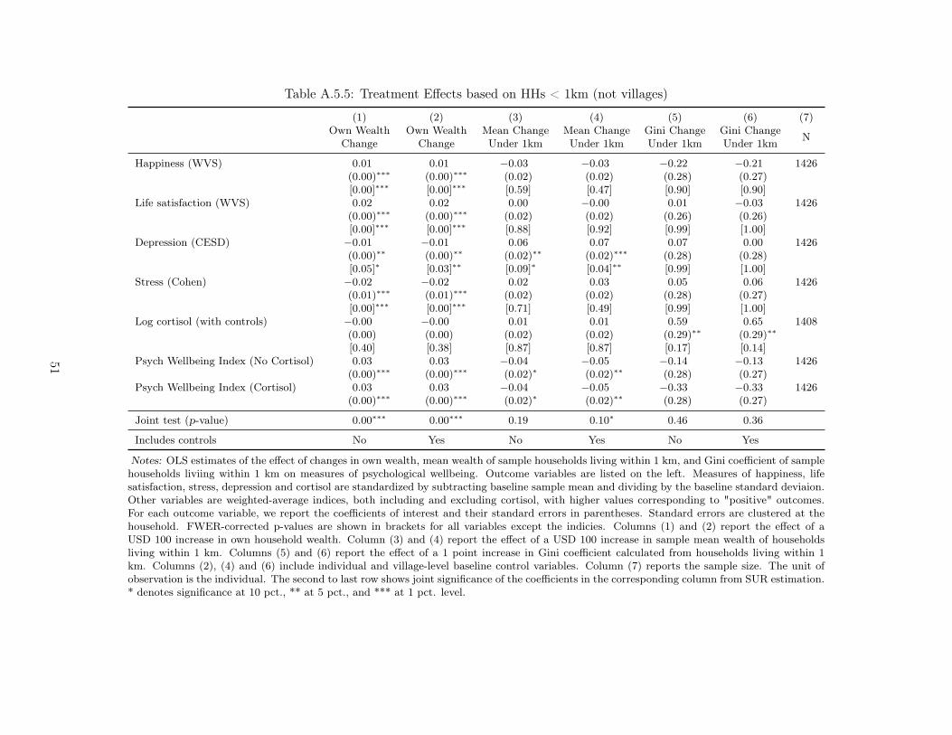
Table A.5.5: Treatment Effects based on HHs < 1km (not villages)

(1) (2) (3) (4) (5) (6) (7)Own Wealth

ChangeOwn Wealth

ChangeMean ChangeUnder 1km

Mean ChangeUnder 1km

Gini ChangeUnder 1km

Gini ChangeUnder 1km N

Happiness (WVS) 0.01 0.01 −0.03 −0.03 −0.22 −0.21 1426(0.00)∗∗∗ (0.00)∗∗∗ (0.02) (0.02) (0.28) (0.27)[0.00]∗∗∗ [0.00]∗∗∗ [0.59] [0.47] [0.90] [0.90]

Life satisfaction (WVS) 0.02 0.02 0.00 −0.00 0.01 −0.03 1426(0.00)∗∗∗ (0.00)∗∗∗ (0.02) (0.02) (0.26) (0.26)[0.00]∗∗∗ [0.00]∗∗∗ [0.88] [0.92] [0.99] [1.00]

Depression (CESD) −0.01 −0.01 0.06 0.07 0.07 0.00 1426(0.00)∗∗ (0.00)∗∗ (0.02)∗∗ (0.02)∗∗∗ (0.28) (0.28)[0.05]∗ [0.03]∗∗ [0.09]∗ [0.04]∗∗ [0.99] [1.00]

Stress (Cohen) −0.02 −0.02 0.02 0.03 0.05 0.06 1426(0.01)∗∗∗ (0.01)∗∗∗ (0.02) (0.02) (0.28) (0.27)[0.00]∗∗∗ [0.00]∗∗∗ [0.71] [0.49] [0.99] [1.00]

Log cortisol (with controls) −0.00 −0.00 0.01 0.01 0.59 0.65 1408(0.00) (0.00) (0.02) (0.02) (0.29)∗∗ (0.29)∗∗

[0.40] [0.38] [0.87] [0.87] [0.17] [0.14]Psych Wellbeing Index (No Cortisol) 0.03 0.03 −0.04 −0.05 −0.14 −0.13 1426

(0.00)∗∗∗ (0.00)∗∗∗ (0.02)∗ (0.02)∗∗ (0.28) (0.27)Psych Wellbeing Index (Cortisol) 0.03 0.03 −0.04 −0.05 −0.33 −0.33 1426

(0.00)∗∗∗ (0.00)∗∗∗ (0.02)∗ (0.02)∗∗ (0.28) (0.27)

Joint test (p-value) 0.00∗∗∗ 0.00∗∗∗ 0.19 0.10∗ 0.46 0.36

Includes controls No Yes No Yes No Yes

Notes: OLS estimates of the effect of changes in own wealth, mean wealth of sample households living within 1 km, and Gini coefficient of samplehouseholds liviing within 1 km on measures of psychological wellbeing. Outcome variables are listed on the left. Measures of happiness, lifesatisfaction, stress, depression and cortisol are standardized by subtracting baseline sample mean and dividing by the baseline standard deviaion.Other variables are weighted-average indices, both including and excluding cortisol, with higher values corresponding to "positive" outcomes.For each outcome variable, we report the coefficients of interest and their standard errors in parentheses. Standard errors are clustered at thehousehold. FWER-corrected p-values are shown in brackets for all variables except the indicies. Columns (1) and (2) report the effect of aUSD 100 increase in own household wealth. Column (3) and (4) report the effect of a USD 100 increase in sample mean wealth of householdsliving within 1 km. Columns (5) and (6) report the effect of a 1 point increase in Gini coefficient calculated from households living within 1km. Columns (2), (4) and (6) include individual and village-level baseline control variables. Column (7) reports the sample size. The unit ofobservation is the individual. The second to last row shows joint significance of the coefficients in the corresponding column from SUR estimation.* denotes significance at 10 pct., ** at 5 pct., and *** at 1 pct. level.

51

Table A.5.6: Subtracting out the Effect of Change in Own Wealth

(1) (2) (3) (4) (5)Village

Mean ChangeVillage

Mean ChangeGini

ChangeGini

Change N

Happiness (WVS) 0.01 0.01 −0.32 −0.14 1474(0.04) (0.03) (0.34) (0.28)[0.98] [0.92] [0.88] [0.97]

Life satisfaction (WVS) −0.06 −0.08 0.14 0.38 1474(0.05) (0.04)∗ (0.47) (0.45)[0.63] [0.33] [0.92] [0.91]

Depression (CESD) −0.02 −0.02 0.26 0.10 1474(0.04) (0.04) (0.46) (0.46)[0.98] [0.92] [0.90] [0.97]

Stress (Cohen) 0.01 0.03 0.38 0.21 1474(0.04) (0.05) (0.42) (0.45)[0.98] [0.92] [0.88] [0.97]

Log cortisol (with controls) 0.00 −0.01 0.16 0.06 1456(0.04) (0.03) (0.40) (0.39)[0.98] [0.92] [0.92] [0.97]

Psychological Wellbeing Index −0.01 −0.02 −0.38 −0.08 1474(0.05) (0.04) (0.50) (0.47)

Joint test (p-value) 0.57 0.29 0.70 0.79

Includes controls No Yes No Yes

Notes: OLS estimates of the effect of changes in own wealth, thatched village mean wealth,and thatched village coefficient of variation on measures of psychological wellbeing. Outcomevariables are listed on the left. Measures of happiness, life satisfaction, stress, depression andcortisol are standardized by subtracting baseline sample mean and dividing by the baselinestandard deviaion. Other variables are weighted-average indices, both including and excludingcortisol, with higher values corresponding to "positive" outcomes. For each outcome variable, wereport the coefficients of interest and their standard errors in parentheses. Standard errors areclustered at the village level. FWER-corrected p-values are shown in brackets for all variablesexcept the indicies. Columns (2), (4) and (6) include individual and village-level baseline controlvariables. Column (7) reports the sample size. The unit of observation is the individual. Thesecond to last row shows joint significance of the coefficients in the corresponding column fromSUR estimation. * denotes significance at 10 pct., ** at 5 pct., and *** at 1 pct. level.

52

A.6 Additional outcome variables

53

Table A.6.1: Full Psych Variable Results

(1) (2) (3) (4) (5) (6) (7)Own Wealth

ChangeOwn Wealth

ChangeVillage

Mean ChangeVillage

Mean ChangeGini

ChangeGini

Change N

Happiness (WVS) 0.01 0.01 −0.00 0.00 −0.35 −0.17 1474(0.00)∗∗∗ (0.00)∗∗∗ (0.03) (0.03) (0.34) (0.28)[0.80] [0.84] [0.86] [0.72] [0.82] [0.95]

Life satisfaction (WVS) 0.02 0.02 −0.08 −0.09 0.11 0.34 1474(0.00)∗∗∗ (0.00)∗∗∗ (0.05)∗ (0.04)∗∗ (0.47) (0.45)[0.05]∗ [0.03]∗∗ [0.46] [0.41] [0.42] [0.10]

Depression (CESD) −0.01 −0.01 −0.01 −0.01 0.29 0.13 1474(0.00)∗∗ (0.00)∗∗ (0.04) (0.04) (0.46) (0.46)[0.13] [0.21] [0.86] [0.72] [0.76] [0.89]

Stress (Cohen) −0.03 −0.03 0.03 0.06 0.43 0.26 1474(0.01)∗∗∗ (0.01)∗∗∗ (0.04) (0.05) (0.42) (0.45)[0.00]∗∗∗ [0.01]∗∗∗ [0.56] [0.41] [0.82] [0.95]

Log cortisol (with controls) −0.00 −0.00 0.01 −0.01 0.17 0.07 1456(0.01) (0.01) (0.04) (0.03) (0.40) (0.39)[0.80] [0.84] [0.80] [0.71] [0.82] [0.89]

Optimism (Scheier) 0.01 0.01 −0.03 −0.03 0.09 0.05 1474(0.00)∗∗ (0.00)∗∗ (0.04) (0.03) (0.29) (0.29)[0.13] [0.15] [0.80] [0.72] [0.76] [0.70]

Psych Wellbeing Index 0.03 0.03 −0.04 −0.06 −0.38 −0.08 1474(0.00)∗∗∗ (0.00)∗∗∗ (0.04) (0.04) (0.47) (0.46)

Psych Wellbeing Index 0.03 0.03 −0.04 −0.05 −0.43 −0.14 1474(0.00)∗∗∗ (0.00)∗∗∗ (0.05) (0.04) (0.49) (0.47)

Joint test (p-value) 0.00∗∗∗ 0.00∗∗∗ 0.40 0.17 0.74 0.86

Includes controls No Yes No Yes No Yes

Notes: OLS estimates of the effect of changes in own wealth, thatched village mean wealth, and thatched village inequalityon preferences. Outcome variables are listed on the left. For each outcome variable, we report the coefficients of interest andtheir standard errors in parentheses. Standard errors are clustered at the village level. Columns (1) and (2) report the effectof a USD 100 increase in own household wealth. Column (3) and (4) report the effect of a USD 100 increase in village meanwealth. Columns (5) and (6) report the effect of a increase in thatched village Gini coefficient from 0 to 1. Columns (2),(4) and (6) include individual and village-level baseline control variables. Column (7) reports the sample size. The unit ofobservation is the individual. The second to last row shows joint significance of the coefficients in the corresponding columnfrom SUR estimation. * denotes significance at 10 pct., ** at 5 pct., and *** at 1 pct. level.

54

Table A.6.2: Effect on Preferences

(1) (2) (3) (4) (5) (6) (7)Own Wealth

ChangeOwn Wealth

ChangeVillage

Mean ChangeVillage

Mean ChangeGini

ChangeGini

Change N

Impatience −0.00 −0.00 −0.03 −0.06 −0.61 −0.28 1474(0.01) (0.01) (0.07) (0.06) (0.62) (0.62)[0.80] [0.83] [0.94] [0.55] [0.68] [0.89]

Decreasing impatience 0.01 0.01 0.03 0.08 −0.68 −0.83 1474(0.01) (0.01) (0.06) (0.06) (0.64) (0.69)[0.41] [0.43] [0.94] [0.42] [0.68] [0.57]

Risk aversion 0.01 0.01 −0.01 −0.02 −0.05 −0.05 1474(0.00)∗ (0.00)∗ (0.03) (0.03) (0.28) (0.28)[0.18] [0.19] [0.94] [0.55] [0.84] [0.89]

Joint test (p-value) 0.13 0.16 0.91 0.42 0.59 0.66

Includes controls No Yes No Yes No Yes

Notes: OLS estimates of the effect of changes in own wealth, thatched village mean wealth, and thatched villageinequality on preferences. Outcome variables are listed on the left. For each outcome variable, we report the coefficientsof interest and their standard errors in parentheses. Standard errors are clustered at the village level. Columns (1)and (2) report the effect of a USD 100 increase in own household wealth. Column (3) and (4) report the effect of aUSD 100 increase in village mean wealth. Columns (5) and (6) report the effect of a increase in thatched village Ginicoefficient from 0 to 1. Columns (2), (4) and (6) include individual and village-level baseline control variables. Column(7) reports the sample size. The unit of observation is the individual. The second to last row shows joint significance ofthe coefficients in the corresponding column from SUR estimation. * denotes significance at 10 pct., ** at 5 pct., and*** at 1 pct. level.

55

Table A.6.3: Effect on Consumption

(1) (2) (3) (4) (5) (6) (7)Own Wealth

ChangeOwn Wealth

ChangeVillage

Mean ChangeVillage

Mean ChangeGini

ChangeGini

Change N

Food total (USD) 1.72 1.74 −5.56 −4.88 18.46 −7.61 939(0.45)∗∗∗ (0.46)∗∗∗ (3.12)∗ (2.94) (31.61) (30.05)[0.00]∗∗∗ [0.01]∗∗∗ [0.48] [0.56] [0.99] [1.00]

Alcohol (USD) −0.11 −0.12 0.30 0.40 −0.04 −2.00 939(0.08) (0.09) (0.52) (0.60) (5.12) (5.65)[0.46] [0.34] [0.88] [0.91] [1.00] [1.00]

Tobacco (USD) −0.02 −0.03 0.15 0.23 −0.14 −0.17 939(0.02) (0.02) (0.13) (0.14)∗ (1.46) (1.51)[0.46] [0.34] [0.80] [0.56] [1.00] [1.00]

Medical expenditure past month (USD) 0.18 0.17 −0.31 −0.39 5.43 0.14 939(0.10)∗ (0.10)∗ (0.54) (0.65) (6.42) (6.51)[0.26] [0.34] [0.88] [0.91] [0.97] [1.00]

Medical expenditure, children (USD) 0.03 0.03 0.29 0.19 2.17 0.37 837(0.06) (0.06) (0.46) (0.49) (4.54) (4.41)[0.63] [0.67] [0.88] [0.91] [0.99] [1.00]

Education expenditure (USD) 0.13 0.12 −0.42 −0.52 0.35 −0.35 939(0.05)∗∗ (0.05)∗∗ (0.27) (0.30)∗ (3.40) (2.64)[0.10] [0.17] [0.63] [0.56] [1.00] [1.00]

Social expenditure (USD) 0.19 0.21 −0.49 −0.45 −0.15 −2.25 939(0.05)∗∗∗ (0.06)∗∗∗ (0.22)∗∗ (0.28) (2.92) (3.14)[0.01]∗∗ [0.01]∗∗ [0.24] [0.56] [1.00] [0.99]

Other expenditure (USD) 1.19 1.23 −1.33 −1.34 21.65 9.82 939(0.19)∗∗∗ (0.19)∗∗∗ (1.29) (1.37) (13.49) (13.76)[0.00]∗∗∗ [0.00]∗∗∗ [0.82] [0.85] [0.64] [0.99]

Home repair (USD) 1.36 1.46 −0.58 −0.33 9.23 10.89 939(0.18)∗∗∗ (0.18)∗∗∗ (0.80) (0.94) (7.21) (7.73)[0.00]∗∗∗ [0.00]∗∗∗ [0.88] [0.91] [0.83] [0.77]

Non-durable expenditure (USD) 3.40 3.35 −7.93 −7.23 42.76 −2.56 939(0.68)∗∗∗ (0.68)∗∗∗ (4.33)∗ (4.29)∗ (46.77) (42.91)[0.00]∗∗∗ [0.00]∗∗∗ [0.44] [0.56] [0.95] [1.00]

Joint test (p-value) 0.00∗∗∗ 0.00∗∗∗ 0.03∗∗ 0.07∗ 0.76 0.94

Includes controls No Yes No Yes No Yes

Notes: OLS estimates of the effect of changes in own wealth, thatched village mean wealth, and thatched village inequality on measuresof household monthly consumption at endline reported in USD PPP. Outcome variables are listed on the left. For each outcome variable,we report the coefficients of interest and their standard errors in parentheses. Standard errors are clustered at the village level. Columns(1) and (2) report the effect of a USD 100 increase in own household wealth. Column (3) and (4) report the effect of a USD 100 increasein village mean wealth. Columns (5) and (6) report the effect of a increase in thatched village Gini coefficient from 0 to 1. Columns (2),(4) and (6) include household and village-level baseline control variables. Column (7) reports the sample size. The unit of observationis the household. The second to last row shows joint significance of the coefficients in the corresponding column from SUR estimation.* denotes significance at 10 pct., ** at 5 pct., and *** at 1 pct. level.

56

Table A.6.4: Effect on Assets

(1) (2) (3) (4) (5) (6) (7)Own Wealth

ChangeOwn Wealth

ChangeVillage

Mean ChangeVillage

Mean ChangeGini

ChangeGini

Change N

Value of non-land assets (USD) 31.93 34.44 −32.78 −36.05 −24.56 −93.00 939(3.48)∗∗∗ (3.30)∗∗∗ (18.27)∗ (18.57)∗ (206.13) (187.63)[0.00]∗∗∗ [0.00]∗∗∗ [0.34] [0.26] [0.93] [0.94]

Value of livestock (USD) 8.32 8.87 −8.80 −13.82 121.15 96.40 939(1.76)∗∗∗ (1.80)∗∗∗ (8.75) (9.83) (90.25) (86.96)[0.00]∗∗∗ [0.00]∗∗∗ [0.81] [0.52] [0.63] [0.73]

Value of durable goods (USD) 6.28 6.69 −8.76 −9.76 19.01 −14.18 939(1.05)∗∗∗ (0.96)∗∗∗ (5.42) (5.33)∗ (56.73) (53.52)[0.00]∗∗∗ [0.00]∗∗∗ [0.42] [0.30] [0.93] [0.94]

Value of savings (USD) 1.12 1.22 −0.53 −0.01 16.39 7.60 939(0.28)∗∗∗ (0.29)∗∗∗ (1.64) (1.84) (15.53) (19.31)[0.00]∗∗∗ [0.00]∗∗∗ [0.81] [0.99] [0.76] [0.94]

Land owned (acres) 0.02 0.02 0.06 0.14 −1.07 −1.61 939(0.02) (0.02) (0.10) (0.11) (1.02) (1.06)[0.46] [0.45] [0.81] [0.52] [0.76] [0.50]

Has non-thatched roof (dummy) 0.03 0.03 −0.02 −0.02 −0.29 −0.24 939(0.00)∗∗∗ (0.00)∗∗∗ (0.02) (0.02) (0.20) (0.22)[0.00]∗∗∗ [0.00]∗∗∗ [0.81] [0.76] [0.58] [0.73]

Joint test (p-value) 0.00∗∗∗ 0.00∗∗∗ 0.31 0.13 0.04∗∗ 0.41

Includes controls No Yes No Yes No Yes

Notes: OLS estimates of the effect of changes in own wealth, thatched village mean wealth, and thatched village inequality onmeasures of household endline assets reported in USD PPP. Outcome variables are listed on the left. For each outcome variable, wereport the coefficients of interest and their standard errors in parentheses. Standard errors are clustered at the village level. Columns(1) and (2) report the effect of a USD 100 increase in own household wealth. Column (3) and (4) report the effect of a USD 100increase in village mean wealth. Columns (5) and (6) report the effect of a increase in thatched village Gini coefficient from 0 to1. Columns (2), (4) and (6) include household and village-level baseline control variables. Column (7) reports the sample size. Theunit of observation is the household. The second to last row shows joint significance of the coefficients in the corresponding columnfrom SUR estimation. * denotes significance at 10 pct., ** at 5 pct., and *** at 1 pct. level.

57

Table A.6.5: Effect on Labor and Enterprise

(1) (2) (3) (4) (5) (6) (7)Own Wealth

ChangeOwn Wealth

ChangeVillage

Mean ChangeVillage

Mean ChangeGini

ChangeGini

Change N

Wage labor primary income (dummy) 0.00 0.00 0.01 0.01 −0.44 −0.51 939(0.00) (0.00) (0.02) (0.02) (0.19)∗∗ (0.19)∗∗∗

[0.99] [0.99] [0.91] [0.89] [0.13] [0.05]∗∗

Own farm primary income (dummy) 0.00 0.00 0.02 0.03 0.10 0.18 939(0.00) (0.00) (0.03) (0.03) (0.33) (0.31)[0.99] [0.99] [0.86] [0.62] [0.94] [0.90]

Non-ag business primary income (dummy) 0.00 0.00 −0.02 −0.03 0.12 0.07 939(0.00) (0.00) (0.01)∗ (0.02)∗ (0.15) (0.15)[0.95] [0.91] [0.32] [0.36] [0.87] [0.90]

Total revenue, monthly (USD) 1.02 1.10 −6.11 −6.15 24.19 2.10 939(0.53)∗ (0.58)∗ (4.07) (4.61) (39.19) (40.29)[0.25] [0.24] [0.45] [0.53] [0.88] [0.94]

Total expenses, monthly (USD) 0.85 0.99 −5.62 −5.99 43.04 32.21 939(0.40)∗∗ (0.44)∗∗ (2.73)∗∗ (2.82)∗∗ (25.73)∗ (27.01)[0.21] [0.15] [0.23] [0.19] [0.37] [0.68]

Total profit, monthly (USD) −0.09 −0.14 −0.82 −0.34 −6.40 −19.34 939(0.25) (0.28) (2.10) (2.74) (22.60) (24.79)[0.99] [0.92] [0.91] [0.91] [0.94] [0.88]

Joint test (p-value) 0.01∗∗ 0.00∗∗∗ 0.32 0.39 0.02∗∗ 0.00∗∗∗

Includes controls No Yes No Yes No Yes

Notes: OLS estimates of the effect of changes in own wealth, thatched village mean wealth, and thatched village inequality on measures ofhousehold endline enterpise measures. Outcome variables are listed on the left. For measures of primary income source, outcomes are discrete,and thus coefficients report the increase in probability of that source being the household’s main income source. Revenue, profit and expenses aremeasured per USD 100. For each outcome variable, we report the coefficients of interest and their standard errors in parentheses. Standard errorsare clustered at the village level. Columns (1) and (2) report the effect of a USD 100 increase in own household wealth. Column (3) and (4) reportthe effect of a USD 100 increase in village mean wealth. Columns (5) and (6) report the effect of a increase in thatched village Gini coefficient from0 to 1. Columns (2), (4) and (6) include household and village-level baseline control variables. Column (7) reports the sample size. The unit ofobservation is the household. The second to last row shows joint significance of the coefficients in the corresponding column from SUR estimation.* denotes significance at 10 pct., ** at 5 pct., and *** at 1 pct. level.

58

Table A.6.6: Gender Violence

(1) (2) (3) (4) (5) (6) (7)Own Wealth

ChangeOwn Wealth

ChangeVillage

Mean ChangeVillage

Mean ChangeGini

ChangeGini

Change N

Physical violence (dummy) −0.00 −0.00 −0.02 −0.02 0.00 0.04 698(0.00) (0.00) (0.03) (0.02) (0.23) (0.24)[0.79] [0.63] [0.61] [0.59] [0.99] [1.00]

Sexual violence (dummy) −0.00 −0.00 −0.01 −0.01 0.04 0.08 698(0.00)∗ (0.00)∗∗ (0.01) (0.02) (0.15) (0.16)[0.33] [0.13] [0.61] [0.59] [0.99] [0.94]

Emotional violence (dummy) 0.00 0.00 −0.04 −0.04 0.03 0.02 698(0.00) (0.00) (0.01)∗∗∗ (0.01)∗∗∗ (0.15) (0.15)[0.43] [0.40] [0.04]∗∗ [0.03]∗∗ [0.99] [1.00]

Justifiability of violence (dummy) −0.00 −0.00 −0.06 −0.04 0.29 0.16 698(0.00) (0.00) (0.02)∗∗∗ (0.02)∗ (0.22) (0.20)[0.79] [0.63] [0.04]∗∗ [0.31] [0.65] [0.88]

Female empowerment index 0.01 0.01 0.16 0.16 −0.67 −0.82 698(0.01) (0.01)∗ (0.04)∗∗∗ (0.05)∗∗∗ (0.57) (0.57)

Joint test (p-value) 0.06∗ 0.07∗ 0.00∗∗∗ 0.01∗∗∗ 0.74 0.90

Includes controls No Yes No Yes No Yes

Notes: OLS estimates of the effect of changes in own wealth, thatched village mean wealth, and thatched village inequality onpreferences. Outcome variables are listed on the left. For each outcome variable, we report the coefficients of interest and theirstandard errors in parentheses. Standard errors are clustered at the village level. Columns (1) and (2) report the effect of aUSD 100 increase in own household wealth. Column (3) and (4) report the effect of a USD 100 increase in village mean wealth.Columns (5) and (6) report the effect of a increase in thatched village Gini coefficient from 0 to 1. Columns (2), (4) and (6)include individual and village-level baseline control variables. Column (7) reports the sample size. The unit of observation is theindividual. The second to last row shows joint significance of the coefficients in the corresponding column from SUR estimation.* denotes significance at 10 pct., ** at 5 pct., and *** at 1 pct. level.

59

Table A.6.7: Gender Violence

(1) (2) (3) (4) (5) (6)

Own WealthChange

Village MeanChange from

Transfers to Men

Village MeanChange from

Transfers to Women

GiniChange

p-value(2)=(3) N

Physical violence (dummy) −0.00 −0.02 −0.03 0.05 0.85 698(0.00) (0.03) (0.02) (0.24)[0.73] [0.71] [0.58] [0.99]

Sexual violence (dummy) −0.00 −0.01 −0.02 0.08 0.41 698(0.00)∗∗ (0.02) (0.02) (0.16)[0.22] [0.80] [0.58] [0.91]

Emotional violence (dummy) 0.00 −0.04 −0.04 0.01 0.85 698(0.00) (0.02)∗∗ (0.02)∗∗ (0.15)[0.51] [0.16] [0.14] [0.99]

Justifiability of violence (dummy) −0.00 −0.06 −0.03 0.15 0.26 698(0.00) (0.03)∗∗ (0.03) (0.20)[0.73] [0.16] [0.58] [0.91]

Female empowerment index 0.01 0.15 0.17 −0.83 0.75 698(0.01)∗ (0.05)∗∗∗ (0.05)∗∗∗ (0.57)

Joint test (p-value) 0.07∗ 0.02∗∗ 0.04∗∗ 0.92

Notes: OLS estimates of the effect of changes in own wealth, thatched village mean wealth, and thatched village inequalityon preferences. Outcome variables are listed on the left. For each outcome variable, we report the coefficients of interestand their standard errors in parentheses. Standard errors are clustered at the village level. Columns (1) and (2) report theeffect of a USD 100 increase in own household wealth. Column (3) and (4) report the effect of a USD 100 increase in villagemean wealth. Columns (5) and (6) report the effect of a increase in thatched village Gini coefficient from 0 to 1. Columns(2), (4) and (6) include individual and village-level baseline control variables. Column (7) reports the sample size. Theunit of observation is the individual. The second to last row shows joint significance of the coefficients in the correspondingcolumn from SUR estimation. * denotes significance at 10 pct., ** at 5 pct., and *** at 1 pct. level.

60

Table A.6.8: Gender Violence

(1) (2) (3) (4) (5) (6)

Own WealthChange

Village MeanChange from

Transfers to Men

Village MeanChange from

Transfers to Women

GiniChange

p-value(2)=(3) N

Happiness (WVS) 0.01 −0.00 0.01 −0.18 0.81 1474(0.00)∗∗∗ (0.04) (0.03) (0.28)[0.00]∗∗∗ [0.98] [0.96] [0.99]

Life satisfaction (WVS) 0.02 −0.16 −0.05 0.26 0.02∗∗ 1474(0.00)∗∗∗ (0.05)∗∗∗ (0.04) (0.41)[0.00]∗∗∗ [0.02]∗∗ [0.70] [0.99]

Depression (CESD) −0.01 0.02 −0.02 0.14 0.49 1474(0.01)∗∗ (0.05) (0.04) (0.45)[0.05]∗ [0.98] [0.93] [0.99]

Stress (Cohen) −0.03 0.04 0.06 0.26 0.75 1474(0.01)∗∗∗ (0.06) (0.05) (0.44)[0.00]∗∗∗ [0.90] [0.70] [0.99]

Log cortisol (with controls) −0.00 −0.01 −0.01 0.06 0.88 1456(0.01) (0.05) (0.04) (0.38)[0.42] [0.98] [0.96] [0.99]

Psychological Wellbeing Index 0.03 −0.08 −0.03 −0.18 0.21 1474(0.00)∗∗∗ (0.05) (0.04) (0.45)

Joint test (p-value) 0.00∗∗∗ 0.02∗∗ 0.62 0.78

Notes: OLS estimates of the effect of changes in own wealth, thatched village mean wealth, and thatched village inequalityon preferences. Outcome variables are listed on the left. For each outcome variable, we report the coefficients of interestand their standard errors in parentheses. Standard errors are clustered at the village level. Columns (1) and (2) report theeffect of a USD 100 increase in own household wealth. Column (3) and (4) report the effect of a USD 100 increase in villagemean wealth. Columns (5) and (6) report the effect of a increase in thatched village Gini coefficient from 0 to 1. Columns(2), (4) and (6) include individual and village-level baseline control variables. Column (7) reports the sample size. Theunit of observation is the individual. The second to last row shows joint significance of the coefficients in the correspondingcolumn from SUR estimation. * denotes significance at 10 pct., ** at 5 pct., and *** at 1 pct. level.

61

A.7 Construction of indices

We construct indices for several of our groups of outcome variables. To this end, we follow theprocedure proposed by Anderson (2008), which is reproduced below:

First, for each outcome variable yjk, where j indices the outcome group and k indices variables withinoutcome groups, we re-code the variable such that high values correspond to positive outcomes.

We then compute the covariance matrix Σj for outcomes in outcome group j, which consists ofelements:

Σjmn =

Njmn∑i=1

yijm − yjmσyjm

yijn − yjnσyjn

(6)

Here, Njmn is the number of non-missing observations for outcomes m and n in outcome group j,yjm and yjn are the means for outcomes m and n, respectively, in outcome group j, and σyjm andσyjn are the standard deviations in the pure control group for the same outcomes.

Next, we invert the covariance matrix, and define weight wjk for each outcome k in outcome group jby summing the entries in the row of the inverted covariance matrix corresponding to that outcome:

Σ−1j =

cj11 cj12 · · · cj1K

cj21 cj22 · · · · · ·...

.... . . . . .

cjK1...

. . . cjKK

(7)

wjk =

Kj∑l=1

cjkl (8)

Here, Kj is the total number of outcome variables in outcome group j. Finally, we transform eachoutcome variable by subtracting its mean and dividing by the control group standard deviation, andthen weighting it with the weights obtained as described above. We denote the result yij becausethis transformation yields a generalized least squares estimator (Anderson 2008).

yij =

∑k∈Kij

wjk

−1 ∑k∈Kij

wjkyijk − yjk

σyjk(9)

Here, Kij denotes the set of non-missing outcomes for observation i in outcome group j.

A.8 Family-wise Error Rate

We adjust the p-values of our coefficients of interest for multiple statistical inference. To this end,we proceed as follows, reproduced again from Anderson (2008). A similar procedure is described inLee & Shaikh (2013) and Romano & Wolf (2005).

62

First, we compute naïve p-values for all index variables yj of our j main outcome groups, and sortthese p-values in ascending order, i.e. such that p1 < p2 < · · · < pJ .

Second, we follow Anderson’s (2008) variant of Efron & Tibshirani’s (1993) non-parametric permu-tation test: for each variable yj of our j main outcome groups, we randomly permute the treatmentassignments across the entire sample, and estimate the model of interest to obtain the p-value for thecoefficient of interest. We enforce monotonicity in the resulting vector of p-values [p∗1, p

∗2, · · · p∗J ]′

by computing p∗∗r = min{p∗r , p∗r+1, · · · p∗J}, where r is the position of the outcome in the vector ofnaïve p-values.

We then repeat this procedure 10,000 times. The non-parametric p-value, pfwer∗r , for each outcomeis the fraction of iterations on which the simulated p-value is smaller than the observed p-value.Finally we enforce monotonicity again: pfwerr = min{pfwer∗r , pfwer∗r+1 , · · · pfwer∗J }. This yields thefinal vector of family-wise error-rate corrected p-values. We will report both these p-values and thenaïve p-values.

63