Embed Size (px)
Citation preview
3-D sound propagation in a shallow ocean
3-D acoustic effects from shelfbreak fronts and
submarine canyons
Ying-Tsong Lin, James F. Lynch, Timothy F. Duda, Arthur E. Newhall
Woods Hole Oceanographic Instiution
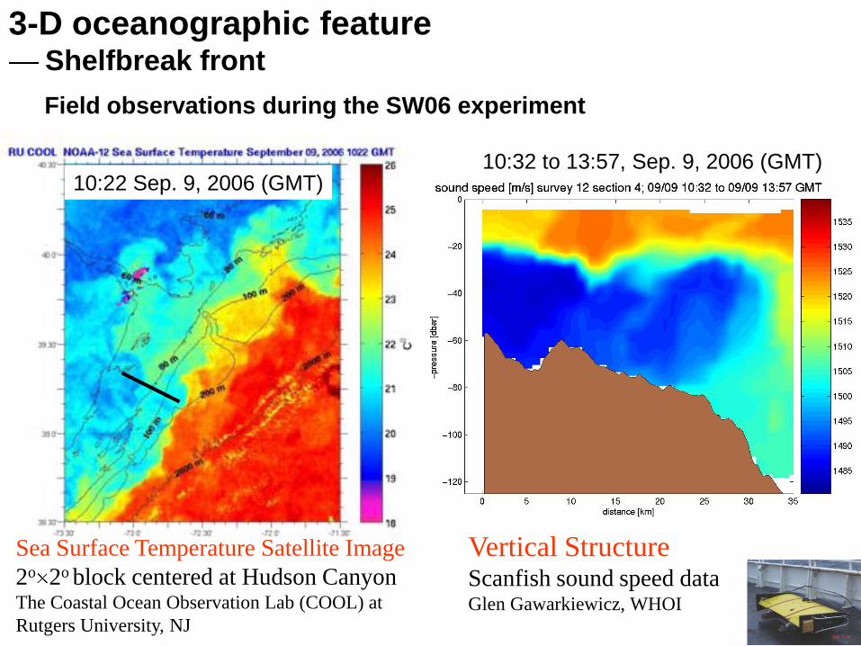
3-D oceanographic featureShelfbreak front
Vertical StructureScanfish sound speed dataGlen Gawarkiewicz, WHOI
Sea Surface Temperature Satellite Image
2o 2o block centered at Hudson CanyonThe Coastal Ocean Observation Lab (COOL) at
Rutgers University, NJ
10:22 Sep. 9, 2006 (GMT)10:32 to 13:57, Sep. 9, 2006 (GMT)
Field observations during the SW06 experiment
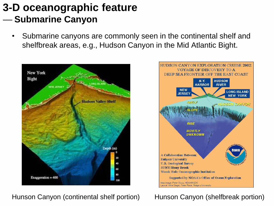
• Submarine canyons are commonly seen in the continental shelf and
shelfbreak areas, e.g., Hudson Canyon in the Mid Atlantic Bight.
3-D oceanographic featureSubmarine Canyon
Hunson Canyon (continental shelf portion) Hunson Canyon (shelfbreak portion)
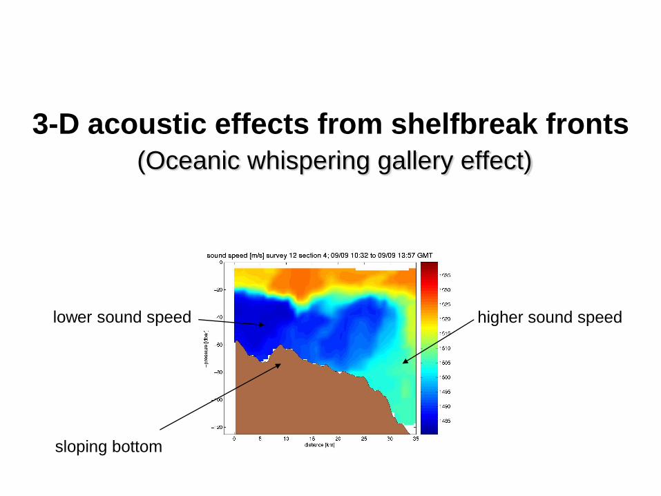
3-D acoustic effects from shelfbreak fronts
(Oceanic whispering gallery effect)
lower sound speed higher sound speed
sloping bottom
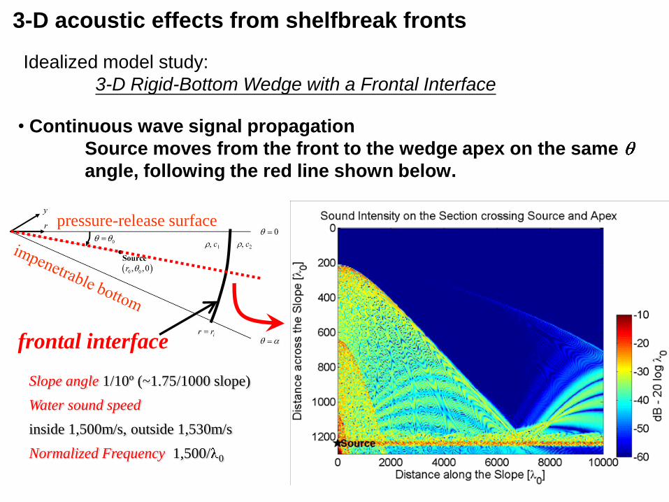
Slope angle 1/10º (~1.75/1000 slope)
Water sound speed
inside 1,500m/s, outside 1,530m/s
Normalized Frequency 1,500/ 0
• Continuous wave signal propagation
Source moves from the front to the wedge apex on the same
angle, following the red line shown below.
frontal interface
3-D acoustic effects from shelfbreak fronts
Idealized model study:
3-D Rigid-Bottom Wedge with a Frontal Interface
pressure-release surface
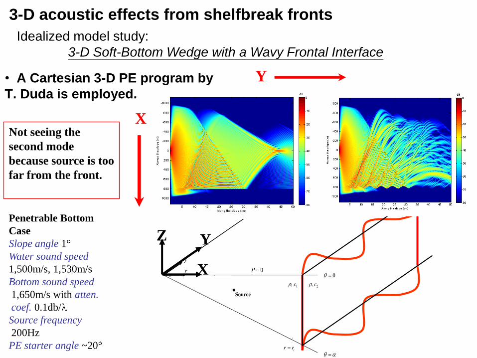
Penetrable Bottom
Case
Slope angle 1
Water sound speed
1,500m/s, 1,530m/s
Bottom sound speed
1,650m/s with atten.
coef. 0.1db/
Source frequency
200Hz
PE starter angle ~20
Not seeing the
second mode
because source is too
far from the front.
X
YZ
3-D acoustic effects from shelfbreak fronts
• A Cartesian 3-D PE program by
T. Duda is employed.
Idealized model study:
3-D Soft-Bottom Wedge with a Wavy Frontal Interface
Y
X
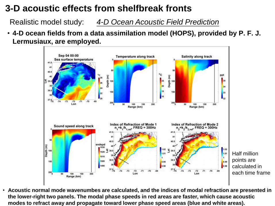
3-D acoustic effects from shelfbreak fronts
• 4-D ocean fields from a data assimilation model (HOPS), provided by P. F. J.
Lermusiaux, are employed.
Realistic model study: 4-D Ocean Acoustic Field Prediction
• Acoustic normal mode wavenumbes are calculated, and the indices of modal refraction are presented in
the lower-right two panels. The modal phase speeds in red areas are faster, which cause acoustic
modes to refract away and propagate toward lower phase speed areas (blue and white areas).
Half million
points are
calculated in
each time frame
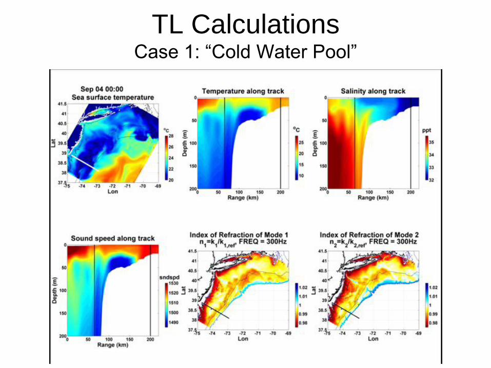
TL CalculationsCase 1: “Cold Water Pool”
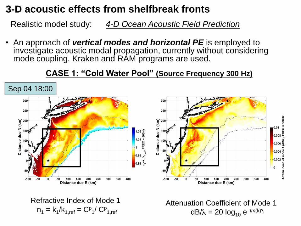
Sep 04 18:00
Refractive Index of Mode 1
n1 = k1/k1,ref = Cp1/ C
p1,ref
Attenuation Coefficient of Mode 1
dB/ = 20 log10 e Im(k)
CASE 1: “Cold Water Pool” (Source Frequency 300 Hz)
Realistic model study: 4-D Ocean Acoustic Field Prediction
• An approach of vertical modes and horizontal PE is employed to investigate acoustic modal propagation, currently without considering mode coupling. Kraken and RAM programs are used.
3-D acoustic effects from shelfbreak fronts
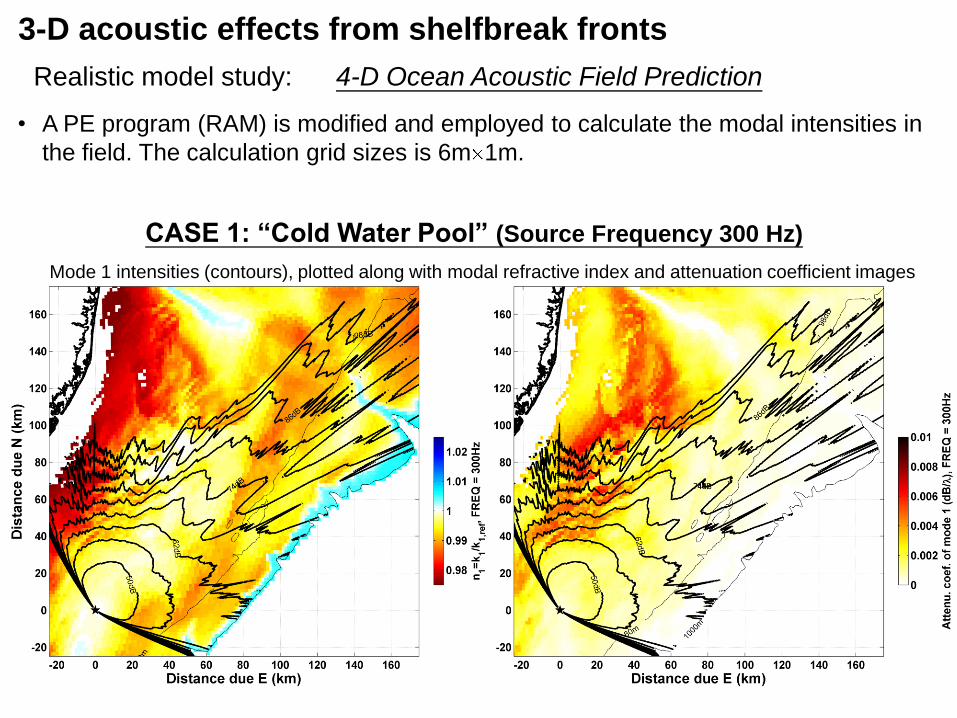
Mode 1 intensities (contours), plotted along with modal refractive index and attenuation coefficient images
CASE 1: “Cold Water Pool” (Source Frequency 300 Hz)
Realistic model study: 4-D Ocean Acoustic Field Prediction
• A PE program (RAM) is modified and employed to calculate the modal intensities in
the field. The calculation grid sizes is 6m 1m.
3-D acoustic effects from shelfbreak fronts
Realistic model study: 4-D Ocean Acoustic Field Prediction
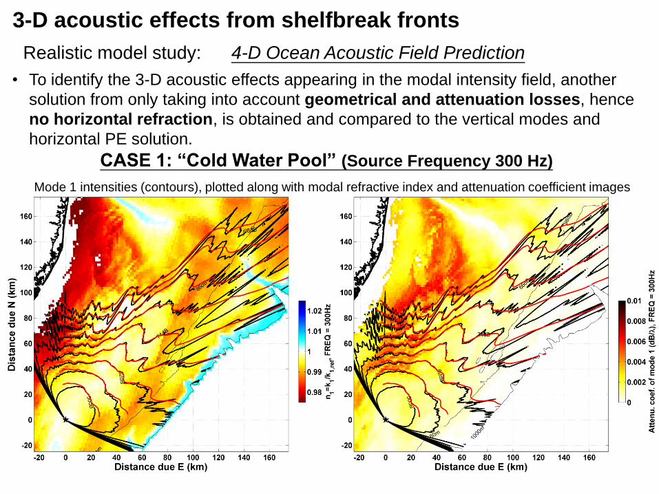
Mode 1 intensities (contours), plotted along with modal refractive index and attenuation coefficient images
CASE 1: “Cold Water Pool” (Source Frequency 300 Hz)
3-D acoustic effects from shelfbreak fronts
• To identify the 3-D acoustic effects appearing in the modal intensity field, another
solution from only taking into account geometrical and attenuation losses, hence
no horizontal refraction, is obtained and compared to the vertical modes and
horizontal PE solution.

TL CalculationsCase 2: Mesoscale Eddy
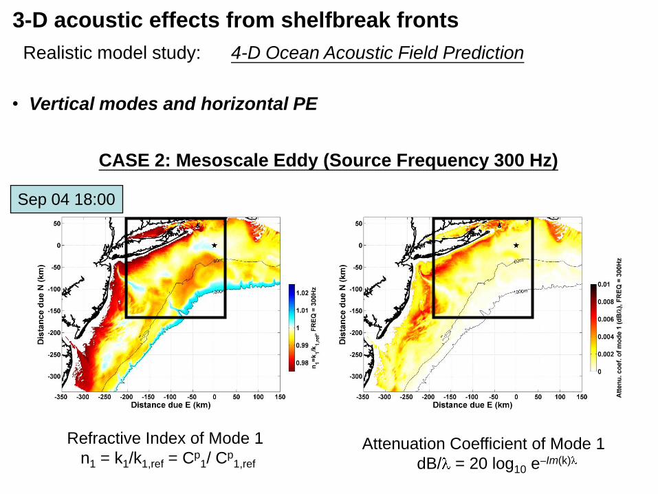
Sep 04 18:00
Refractive Index of Mode 1
n1 = k1/k1,ref = Cp1/ C
p1,ref
Attenuation Coefficient of Mode 1
dB/ = 20 log10 e Im(k)
CASE 2: Mesoscale Eddy (Source Frequency 300 Hz)
Realistic model study: 4-D Ocean Acoustic Field Prediction
• Vertical modes and horizontal PE
3-D acoustic effects from shelfbreak fronts
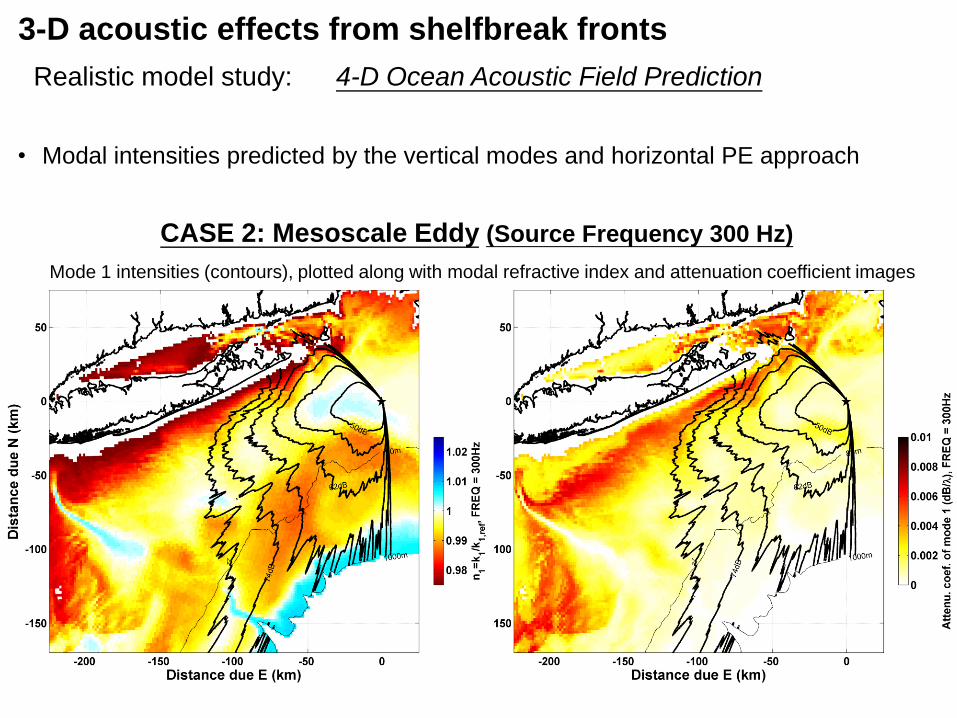
Mode 1 intensities (contours), plotted along with modal refractive index and attenuation coefficient images
CASE 2: Mesoscale Eddy (Source Frequency 300 Hz)
Realistic model study: 4-D Ocean Acoustic Field Prediction
• Modal intensities predicted by the vertical modes and horizontal PE approach
3-D acoustic effects from shelfbreak fronts
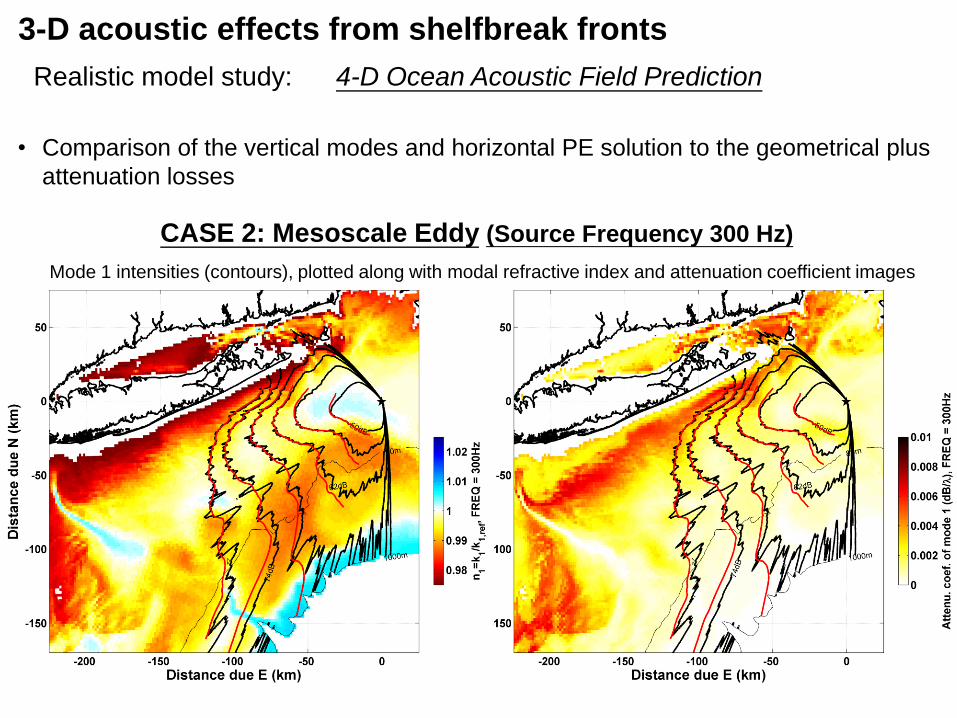
CASE 2: Mesoscale Eddy (Source Frequency 300 Hz)
Mode 1 intensities (contours), plotted along with modal refractive index and attenuation coefficient images
Realistic model study: 4-D Ocean Acoustic Field Prediction
3-D acoustic effects from shelfbreak fronts
• Comparison of the vertical modes and horizontal PE solution to the geometrical plus
attenuation losses

TL CalculationsCase 3: SW06 Acoustic Site
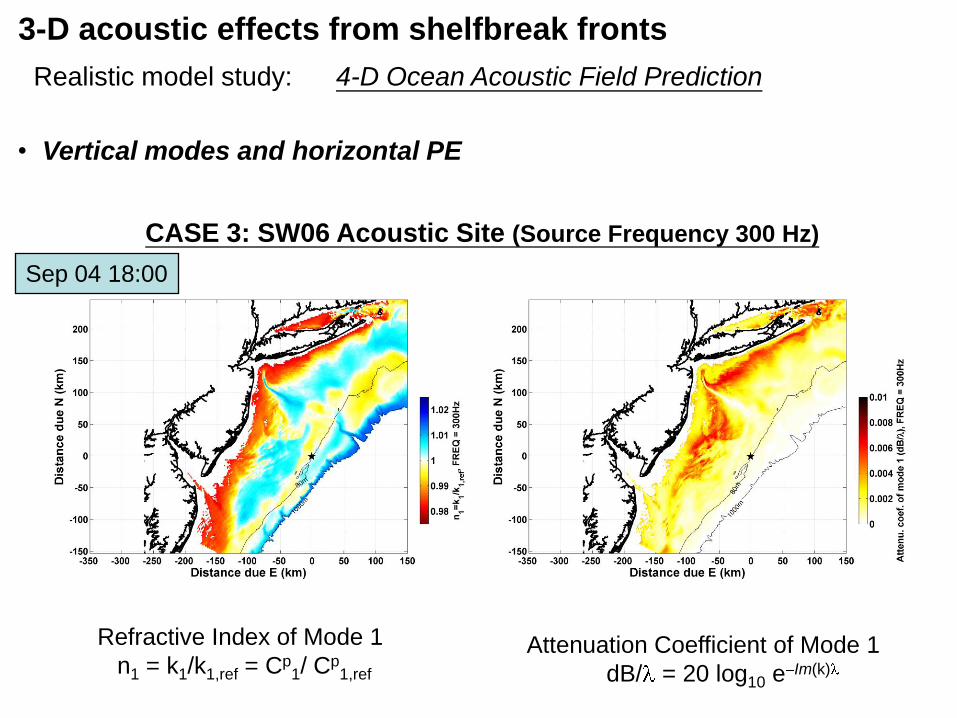
Sep 04 18:00
Refractive Index of Mode 1
n1 = k1/k1,ref = Cp1/ C
p1,ref
Attenuation Coefficient of Mode 1
dB/ = 20 log10 e Im(k)
Realistic model study: 4-D Ocean Acoustic Field Prediction
CASE 3: SW06 Acoustic Site (Source Frequency 300 Hz)
• Vertical modes and horizontal PE
3-D acoustic effects from shelfbreak fronts
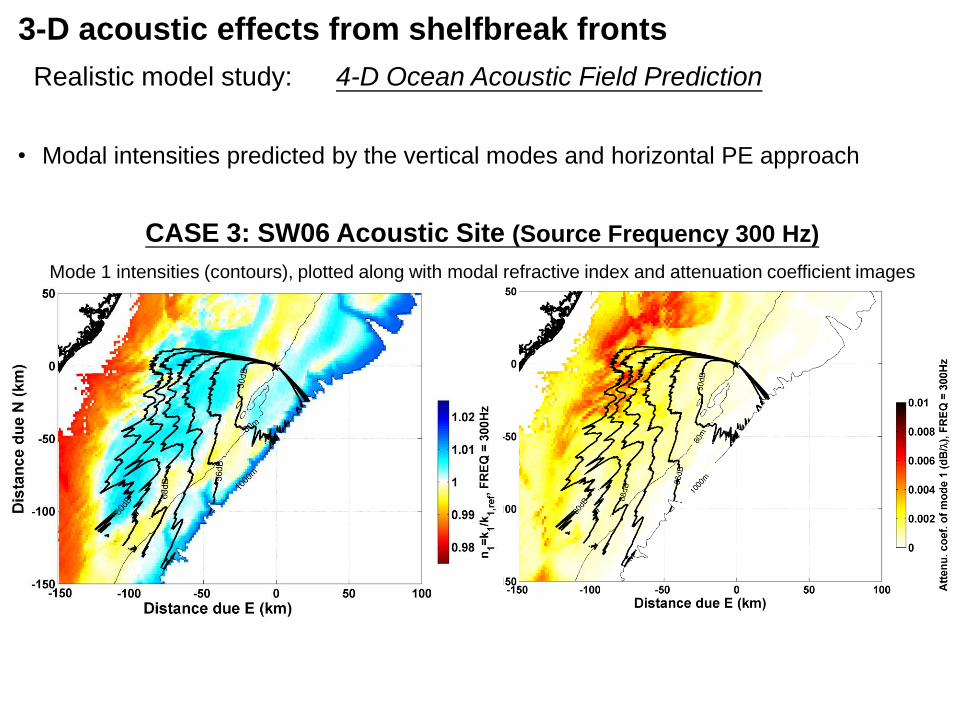
Realistic model study: 4-D Ocean Acoustic Field Prediction
Mode 1 intensities (contours), plotted along with modal refractive index and attenuation coefficient images
• Modal intensities predicted by the vertical modes and horizontal PE approach
3-D acoustic effects from shelfbreak fronts
CASE 3: SW06 Acoustic Site (Source Frequency 300 Hz)
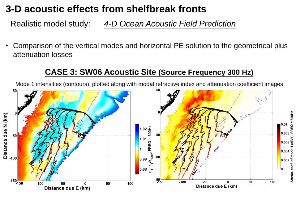
Realistic model study: 4-D Ocean Acoustic Field Prediction
Mode 1 intensities (contours), plotted along with modal refractive index and attenuation coefficient images
• Comparison of the vertical modes and horizontal PE solution to the geometrical plus
attenuation losses
3-D acoustic effects from shelfbreak fronts
CASE 3: SW06 Acoustic Site (Source Frequency 300 Hz)
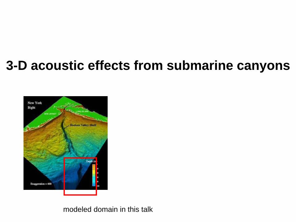
3-D acoustic effects from submarine canyons
modeled domain in this talk
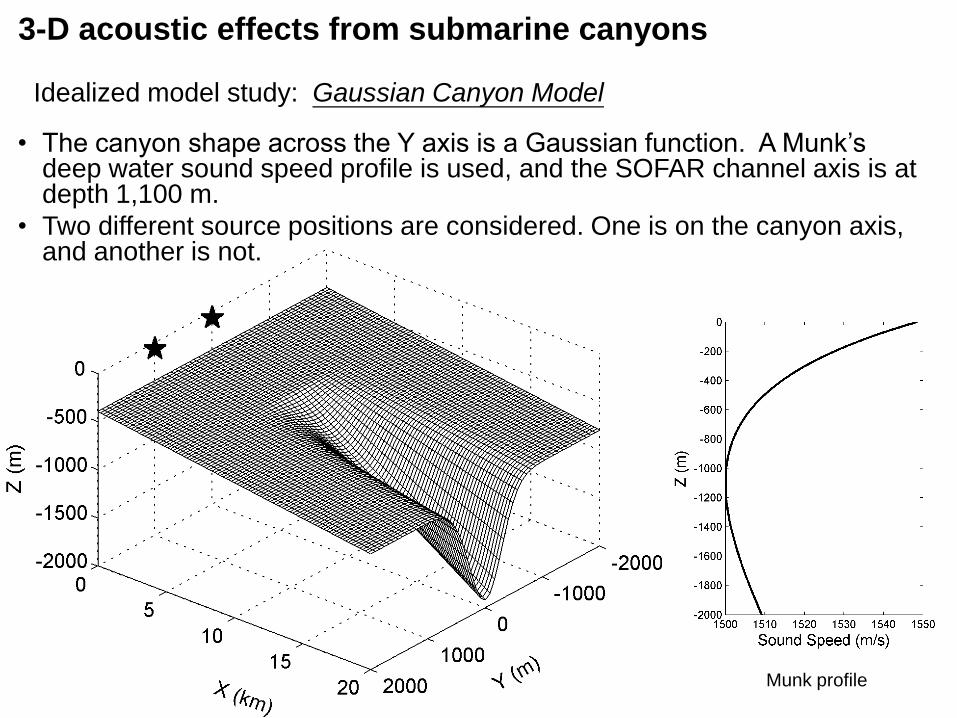
3-D acoustic effects from submarine canyons
Idealized model study: Gaussian Canyon Model
• The canyon shape across the Y axis is a Gaussian function. A Munk’s deep water sound speed profile is used, and the SOFAR channel axis is at depth 1,100 m.
• Two different source positions are considered. One is on the canyon axis, and another is not.
Munk profile
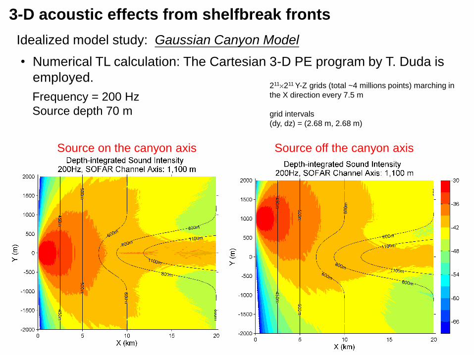
Frequency = 200 Hz
Source depth 70 m
• Numerical TL calculation: The Cartesian 3-D PE program by T. Duda is
employed.
3-D acoustic effects from shelfbreak fronts
Idealized model study: Gaussian Canyon Model
Source on the canyon axis Source off the canyon axis
211 211 Y-Z grids (total ~4 millions points) marching in
the X direction every 7.5 m
grid intervals
(dy, dz) = (2.68 m, 2.68 m)
3-D acoustic effects from submarine canyons
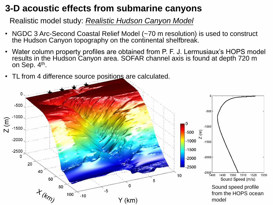
Realistic model study: Realistic Hudson Canyon Model
• NGDC 3 Arc-Second Coastal Relief Model (~70 m resolution) is used to construct the Hudson Canyon topography on the continental shelfbreak.
• Water column property profiles are obtained from P. F. J. Lermusiaux’s HOPS model results in the Hudson Canyon area. SOFAR channel axis is found at depth 720 m on Sep. 4th.
• TL from 4 difference source positions are calculated.
Sound speed profile
from the HOPS ocean
model
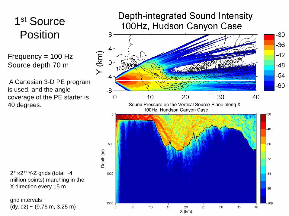
1st Source
Position
Frequency = 100 Hz
Source depth 70 m
A Cartesian 3-D PE program
is used, and the angle
coverage of the PE starter is
40 degrees.
211 211 Y-Z grids (total ~4
million points) marching in the
X direction every 15 m
grid intervals
(dy, dz) ~ (9.76 m, 3.25 m)
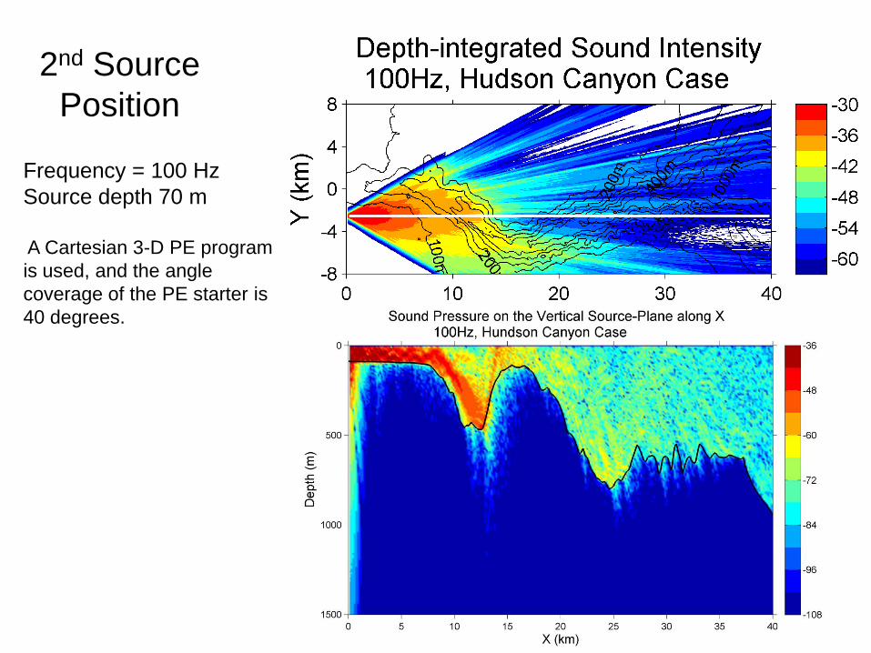
2nd Source
Position
Frequency = 100 Hz
Source depth 70 m
A Cartesian 3-D PE program
is used, and the angle
coverage of the PE starter is
40 degrees.
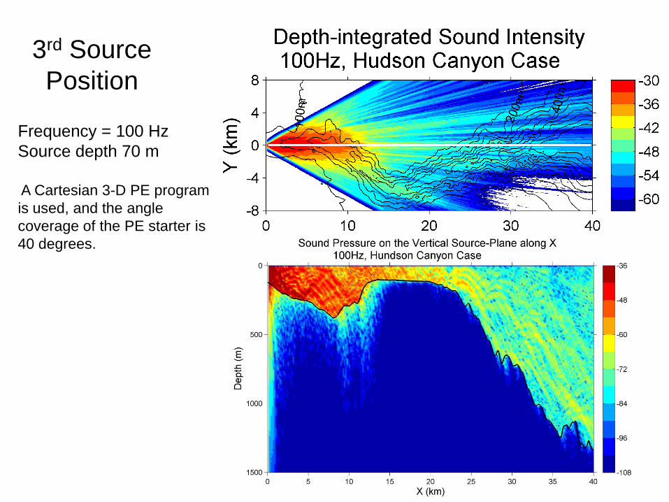
3rd Source
Position
Frequency = 100 Hz
Source depth 70 m
A Cartesian 3-D PE program
is used, and the angle
coverage of the PE starter is
40 degrees.
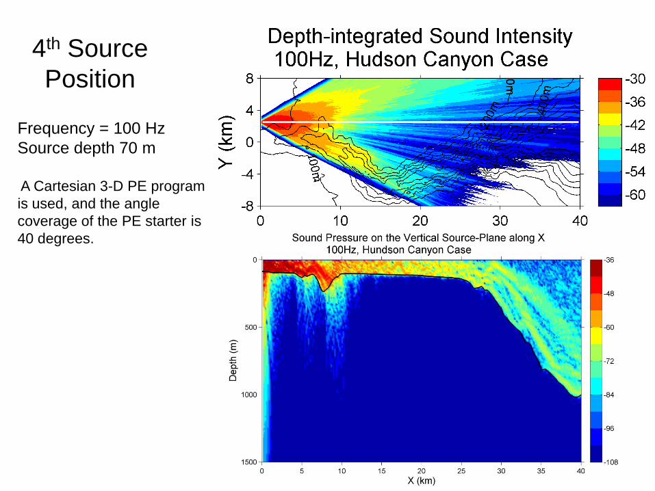
4th Source
Position
Frequency = 100 Hz
Source depth 70 m
A Cartesian 3-D PE program
is used, and the angle
coverage of the PE starter is
40 degrees.
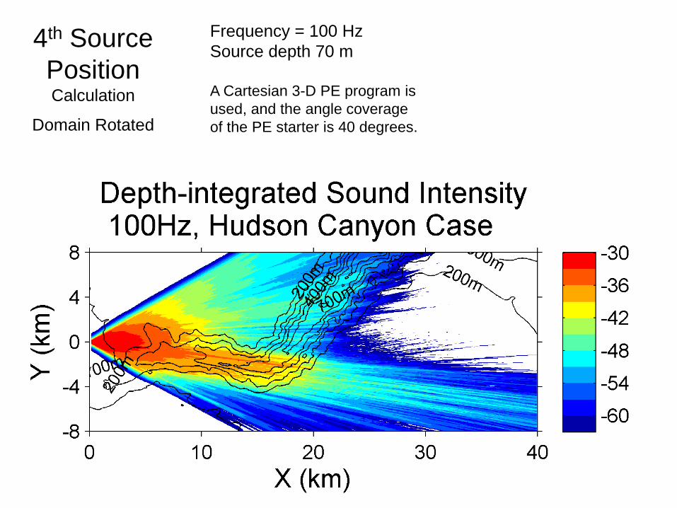
4th Source
PositionCalculation
Domain Rotated
Frequency = 100 Hz
Source depth 70 m
A Cartesian 3-D PE program is
used, and the angle coverage
of the PE starter is 40 degrees.
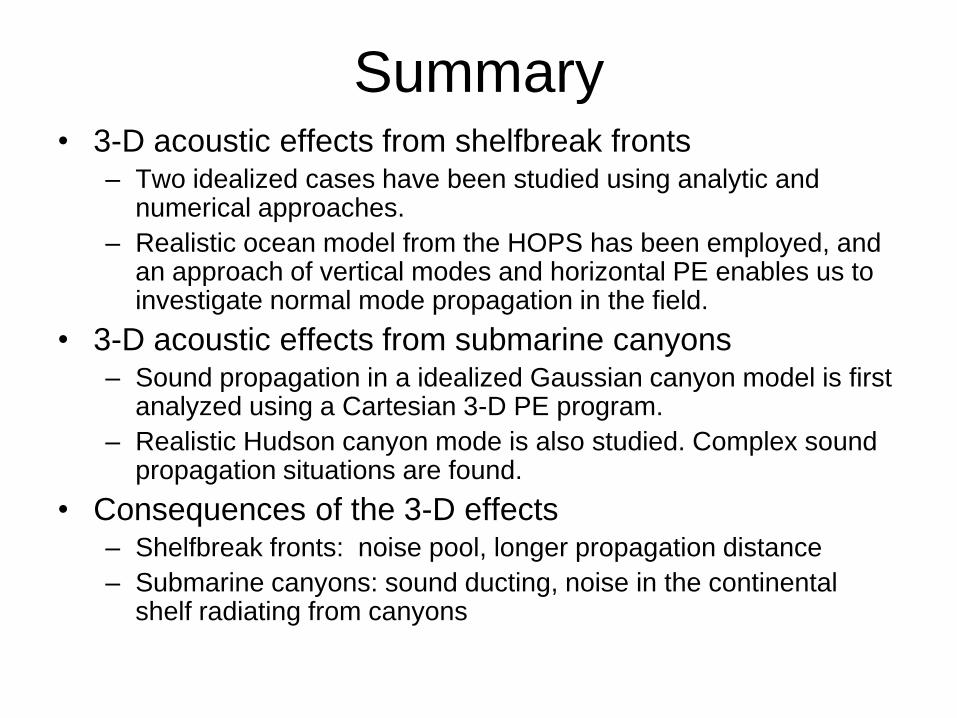
Summary• 3-D acoustic effects from shelfbreak fronts
– Two idealized cases have been studied using analytic and numerical approaches.
– Realistic ocean model from the HOPS has been employed, and an approach of vertical modes and horizontal PE enables us to investigate normal mode propagation in the field.
• 3-D acoustic effects from submarine canyons– Sound propagation in a idealized Gaussian canyon model is first
analyzed using a Cartesian 3-D PE program.
– Realistic Hudson canyon mode is also studied. Complex sound propagation situations are found.
• Consequences of the 3-D effects– Shelfbreak fronts: noise pool, longer propagation distance
– Submarine canyons: sound ducting, noise in the continental shelf radiating from canyons
Backup Slides
wedge
apex
frontal interface
y
rpressure-release surface
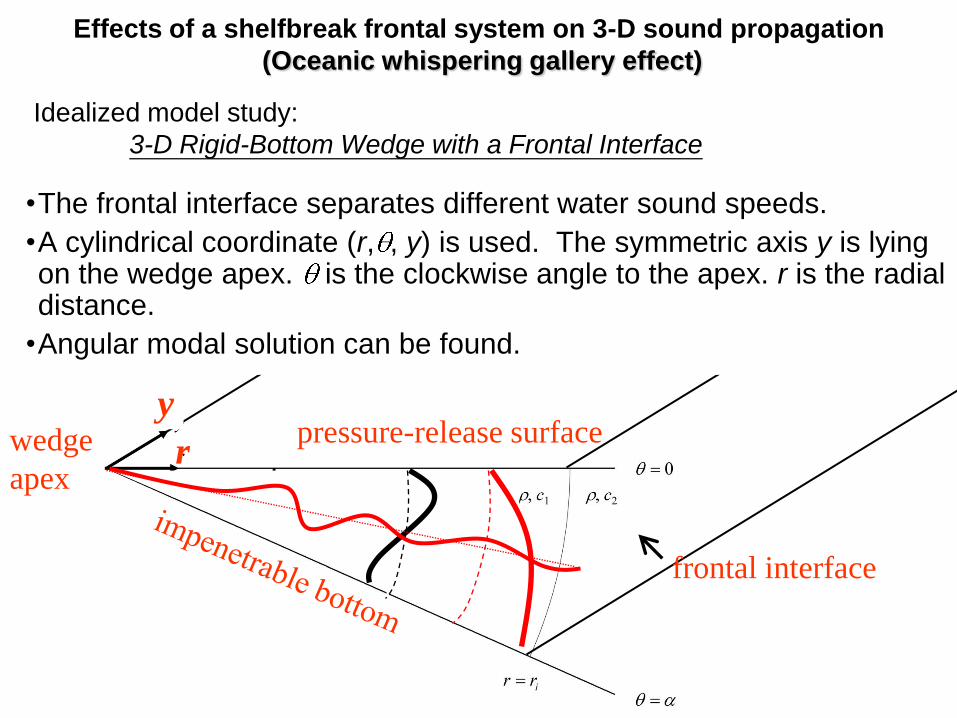
•The frontal interface separates different water sound speeds.
•A cylindrical coordinate (r, , y) is used. The symmetric axis y is lying on the wedge apex. is the clockwise angle to the apex. r is the radial distance.
•Angular modal solution can be found.
Idealized model study:
3-D Rigid-Bottom Wedge with a Frontal Interface
Effects of a shelfbreak frontal system on 3-D sound propagation
(Oceanic whispering gallery effect)
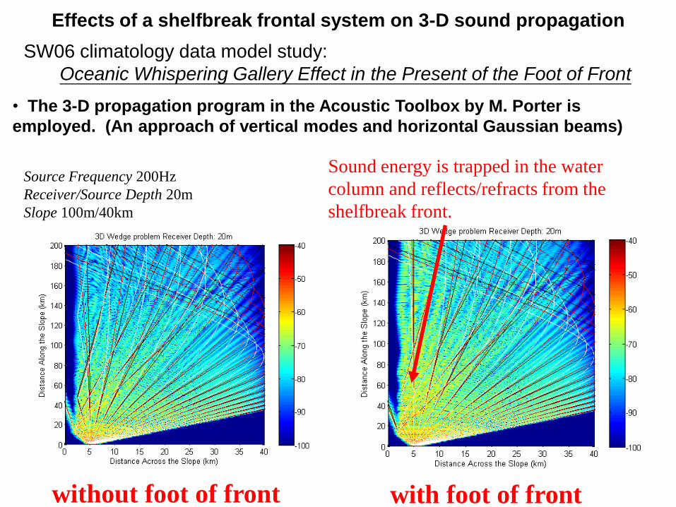
Source Frequency 200Hz
Receiver/Source Depth 20m
Slope 100m/40km
without foot of front with foot of front
Sound energy is trapped in the water
column and reflects/refracts from the
shelfbreak front.
Effects of a shelfbreak frontal system on 3-D sound propagation
SW06 climatology data model study:
Oceanic Whispering Gallery Effect in the Present of the Foot of Front
• The 3-D propagation program in the Acoustic Toolbox by M. Porter is
employed. (An approach of vertical modes and horizontal Gaussian beams)
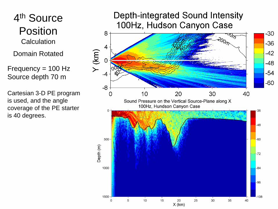
4th Source
PositionCalculation
Domain Rotated
Frequency = 100 Hz
Source depth 70 m
Cartesian 3-D PE program
is used, and the angle
coverage of the PE starter
is 40 degrees.