X-Efficiency and Management Quality in Commercial Banks

Robert DeYoung

Office of the Comptroller of the CurrencyEconomic & Policy Analysis

Working Paper 94-1January 1994

* The opinions expressed in this paper are those of the author and do not necessarily reflect thoseof the Office of the Comptroller of the Currency or the Department of the Treasury. Any wholeor partial reproduction of material in this paper should include the following citation: DeYoung, Robert, “X-Efficiency and Management Quality in Commercial Banks,” Office ofthe Comptroller of the Currency, E&PA Working Paper 94-1, January 1994.

______________________________________________________________________________________

The author thanks Gary Whalen for graciously providing a data set of examination ratings for national banks.

The author also thanks Philip Bartholomew, Allen Berger, Jeffrey Brown, Mike Carhill, Edward Dumas, Alton

Gilbert, Dennis Glennon, Kevin Jacques, Lawrence Leong, Thomas Lutton, and Daniel Nolle for helpful comments,

David Becher for research support, and Claire Emory for editorial assistance. All errors are the responsibility of the

author.

Please address questions to Robert DeYoung, Financial Economist, Bank Research Division, Office of the

Comptroller of the Currency, 250 E Street SW, Washington, DC 20219. Phone (202) 874-5427, Fax (202) 874-

5394, E-mail robert.deyoung@.occ.treas.gov.

These studies are discussed in Section I, "Empirical Literature on Cost Inefficiency in Banks."1

1

* Any whole or partial reproduction of material in this paper should include the followingcitation: DeYoung, Robert, “X-Efficiency and Management Quality in Commercial Banks,”Office of the Comptroller of the Currency, E&PA Working Paper 94-1, January 1994.

Introduction

Econometric studies of banking costs reveal surprisingly large cost differences between

otherwise similar banks. After controlling for differences in size, product mix, number of

branches, and a variety of market factors, these studies typically find that the average bank

incurs costs that are 20 to 25 percent higher than costs at the most efficient banks. These

excess costs are commonly referred to as X-inefficiencies to distinguish them from scale or

scope inefficiencies. Estimates of X-inefficiency are considerably larger than estimates of

scale and scope economies and appear to be comprised mostly of technical inefficiency,

although some studies have also found nontrivial amounts of allocative inefficiency.

A number of empirical studies have found relationships between X-inefficiency and

bank structure, organizational form, and market environment. Studies have found higher1

levels of banking X-inefficiency in states with greater regulatory restrictions, and have also

found that banks in multibank holding company organizations – allegedly formed to

circumvent such restrictions – are more X-inefficient than branch banking organizations.

There is evidence that X-inefficiency is larger in banks where the CEO chairs the board of

directors, perhaps because this arrangement makes monitoring more difficult and reduces the

effectiveness of incentive mechanisms. Some studies have found that X-inefficiency is less

severe in larger banks, perhaps because large banks experience greater pressure from owners

2

concerning bottom-line profits, are better able to attract capable managers, and/or operate in

metropolitan markets that are both more competitive (creating pressure to control costs) and

more densely populated (allowing more efficient delivery systems).

These results suggest a dichotomy: some X-inefficiency occurs because conditions

outside managers' control (e.g., restrictive branching laws, low population density) prevent

them from operating their banks efficiently, while the rest of X-inefficiency is due to, or is

exacerbated by, bad management practices (e.g., managerial laxity when rivalry is not intense,

utility-maximizing behavior by managers). No previous empirical studies have attempted to

separate the proportion of X-inefficiency imposed on managers from the proportion caused by

managers.

This study compares X-inefficiency in well-managed national banks to X-inefficiency in

poorly managed national banks. Because management quality cannot be observed directly,

national banks are assigned to these two groups based on the management component of the

CAMEL rating assigned to them by examiners from the Office of the Comptroller of the

Currency (OCC). The intergroup difference in X-inefficiency is estimated using a thick

frontier cost approach that filters out cost differences that are beyond the control of managers.

The results are compared to estimates of total X-inefficiency in order to approximate the

relative importance of management quality in determining overall X-inefficiency in banks. On

average, poorly managed banks exhibited about 12 percent more X-inefficiency than did well-

managed banks. This result is around two-thirds as large as total X-inefficiency.

Section I summarizes the empirical literature on X-efficiency in banking. Section II

describes how bank examiners assign management quality ratings to banks and shows how

3

these ratings are related to various measures of bank performance. Section III presents the

statistical cost model used to generate estimates of X-inefficiency. Section IV describes the

data. Section V contains preliminary results. Section VI draws some conclusions from the

results and discusses the potential for future research.

I. Empirical Literature on Cost Inefficiency in Banks

The empirical literature on cost efficiency in banks has burgeoned during the past five

years. Berger, Hunter, and Timme (1993) and Evanoff and Israilevich (1991a) contain good

reviews of this literature. In general, these studies find that banks of similar size and product

mix incur widely divergent costs that vary by amounts far larger than the savings available

from scale and scope economies. Many of the studies focus on what Leibenstein (1966) called

"X-inefficiencies," i.e, costs incurred over and above the minimum cost necessary to sustain

output at its current level. Leibenstein coined the term to describe management laxity that

arises in firms with market power, but in the banking cost literature it has come to be used in a

more general sense to describe any excess cost of production not caused by suboptimal scale

or scope.

I.A Estimates of X-Inefficiency in Banks

X-inefficiencies are usually estimated by computing the distance between a bank' s

actual costs and a "frontier-efficient" or "best practices" cost function representing the lower

bound of costs attainable only by the most cost-efficient banks. Empirical studies using these

methods generally control for cost differences due to scale, product mix, branching status, and

4

regional variation in input prices, and often decompose the resulting estimates of X-

inefficiency into technical inefficiency (employing unnecessary inputs or paying above market

prices for inputs) and allocative inefficiency (employing inputs in suboptimal combinations).

Four different techniques, which differ based on maintained assumptions about error

term(s), have been used to generate estimates of X-inefficiency in banks. The econometric

frontier approach (EFA) separates the error term in an econometric cost function into two

components: a symmetric, random disturbance, and a one-sided, nonrandom component that

is assumed to be related to inefficiencies. Using EFA methods, Ferrier and Lovell (1990)

found that costs at the average bank were about 26 percent greater than the frontier,

approximately two-thirds of which was allocative inefficiency, Pi and Timme (1993) found

that the average bank in their sample of large, publicly traded banks incurred controllable

costs that were approximately 11 percent higher than the frontier, and Bauer, Berger, and

Humphrey (1993) found that X-inefficiencies averaged around 16 percent over an 11-year

period.

The thick frontier approach (TFA) uses a priori information on unit costs to select

subsamples of efficient and inefficient banks, then uses standard econometric techniques to

estimate "thick" (as opposed to discrete edges) upper and lower cost boundaries. The error

terms within each of the two subsamples are assumed to reflect only random error and luck,

whereas the difference between the two subsamples is assumed to reflect only inefficiencies

and market factors. This method was pioneered by Berger and Humphrey (1991), who found

that the average bank had unit costs around 25 percent greater than the efficient lower bound,

over two-thirds of which was technical inefficiency. Using the thick frontier approach, Bauer,

5

Berger, and Humphrey (1993) found that X-inefficiencies averaged around 21 percent over an

11-year period.

The distribution-free approach (DFA) generates measures of cost inefficiency using the

residuals from a standard econometric cost model estimated separately over a series of years.

This method assumes that, because the randomness in the error terms will cancel out over

time, the interyear average residual contains only information about X-efficiency. Berger and

Humphrey (1992) used this method to generate an ordinal efficiency index to test for cost

efficiencies in large bank mergers.

Data envelopment analysis (DEA) uses a nonparametric (linear programming) method

to generate a lower envelope of the production function. Since DEA is a nonstochastic

approach, random error is assumed away, and any cost differences due to random events are

included in inefficiency. Using DEA methods, Ferrier and Lovell (1990) found that the

average bank used 21 percent more inputs than necessary, approximately three-quarters of

which was technical inefficiency. Aly, Grabowski, Pasurka, and Rangan (1990) found that

banks could have employed 35 percent fewer inputs without reducing output. Elyasiani and

Mehdian (1990), who used a technique that measured technical but not allocative efficiency,

found that banks overemployed inputs by about 12 percent.

I.B Determinants of Cost Inefficiency in Banks

There are many, non-mutually exclusive explanations for why some banks are more X-

inefficient than others, and the set of empirical studies linking X-inefficiency in commercial

See Berger, Hunter, and Timme (1993, p. 228) and Evanoff and Israilevich (1991a, p. 27) for discussions of theory2

and evidence.

A 1988 OCC study, Bank Failure: An Evaluation of the Factors Contributing to the Failure of National Banks,3

concluded that the predominant cause of bank failure is poor management, but this study did not measure cost

efficiency in these banks.

6

banks to these phenomena is growing. None of these studies, however, tests the relationship2

between management quality and X-efficiency. 3

One line of inquiry focuses on agency theory. Using an EFA approach, Pi and Timme

(1993) found that X-inefficiency in large, publicly traded commercial banks decreased as CEO

stock ownership increased as long as the CEO was not also the chairperson of the board of

directors. When the two positions were consolidated, X-inefficiency increased with the

percentage of the firm owned by the CEO. These results suggest that stock ownership can be

an effective way to reduce owners' monitoring costs and discourage utility-maximizing

behavior by managers, but that such arrangements become ineffective and X-inefficiencies can

result when too much power is concentrated in the hands of the CEO.

Another line of inquiry looks at differences in organizational form across banks. Using

DEA methods, Grabowski, Rangan, and Rezvanian (1993) found that X-inefficiency is larger

in multibank holding companies than in branch banking organizations. The authors conclude

that, to the extent that multibank holding companies are organizational arrangements designed

to circumvent product and geographic market restrictions, removal of regulatory barriers will

improve efficiency in banking markets by reducing X-inefficiency. Newman and Shrieves

(1993) found the opposite – that multibank holding company organizations have about a 2

percent cost advantage over branch banking organizations – although they did not use a cost

frontier approach to estimate their cost model.

7

There is evidence that branching and other restrictions prevent banks from operating as

efficiently as possible. Evanoff and Israilevich (1991b) found that X-inefficiency in large

banks is greater in regions characterized by more restrictive state level regulation, and also

found that X-inefficiency in these banks decreased after the financial deregulation of the early

1980s. Evanoff, Israilevich, and Merris (1990) estimated that inefficiency due to regulation

amounts to about 2 percent of total costs for large commercial banks.

Many of the studies mentioned above compare estimates of X-inefficiency across

institutions of different sizes. Large banks may be more X-efficient than small banks if they

face greater pressure from owners concerning bottom-line profits or are better able to attract

capable managers. In addition, large banks tend to be located in highly competitive, densely

populated metropolitan areas, which may create pressure to control costs and/or require fewer

branch locations to provide a given amount of financial services. Evidence on the relationship

between cost-based X-inefficiency and commercial bank scale is mixed. Aly, et al (1990)

found a positive and statistically significant relationship between scale and only one out of four

alternate measures of X-inefficiency. Berger and Humphrey (1991) found that X-inefficiency

at first falls, then rises, with scale. Bauer, Berger, and Humphrey (1993) found that X-

inefficiency increases with size when using EFA methods, but is not related to size when using

TFA methods. Berger, Hancock, and Humphrey (1993) extended the concept of X-

inefficiency to include output inefficiency (e.g., suboptimal revenues) in addition to cost-based

input inefficiencies and found that this measure of X-inefficiency is negatively related to scale.

Ironically, only one study (to the author' s knowledge) has attempted to find the

negative relationship between X-inefficiency and market rivalry originally hypothesized by

8

Leibenstein. Berger and Humphrey (1992) regressed an ordinal measure of X-inefficiency on

a set of variables that included market concentration and found no relationship between

concentration and X-efficiency. It may not be possible to establish this relationship

empirically given the difficulty of constructing meaningful measures of market concentration

for banks that operate branches (or banking companies that operate banks) in multiple

geographic markets.

It is possible that studies mistakenly identify banks that provide higher quality service

as X-inefficient if high quality services require banks to purchase more and/or more expensive

inputs than banks offering services of lesser quality. However, measurement problems make

it difficult to separate cost-based X-inefficiency from cost-intensive service quality in banking.

Standard measures of service or product quality (e.g., customer turnover, defect rates) are

either not applicable or not available for banks. Available proxies for service quality (e.g.,

FTE labor per deposit account, branches per deposit account) are also not useful, because they

are highly correlated with costs, and hence with X-inefficiency, by construction. Using a

profit function rather than cost function to estimate X-inefficiency might control for levels of

service quality – presumably, the market is willing to pay more for higher quality service –

but separating service quality from other determinants of the resulting estimates of X-

inefficiency would still be difficult.

II. Measuring the Quality of Bank Management

Under the Federal Deposit Insurance Corporation Improvement Act of 1991 (FDICIA),

every commercial bank is examined annually for safety and soundness by either its primary

A small number of banks are examined every 18 months. Banks qualify for this exception if they have less than4

$100 million of assets, have CAMEL ratings of 1, are well capitalized, and have not experienced a change of control

during the previous 12 months.

See OCC Examining Circular 159 (1979) for details of the composite CAMEL rating and its individual5

components.

9

federal regulator (the FDIC, the Federal Reserve System, or the OCC) or by its state

regulator. The most important product of the annual exam is the "CAMEL" rating. The4

CAMEL rating is a composite of five performance dimensions – capital adequacy (C), asset

quality (A), management/administration (M), earnings (E), and liquidity (L) – each of which

ranges in whole numbers from 1 ("strong performance") to 5 ("unsatisfactory"). The5

CAMEL rating also ranges from 1 (".. .basically sound in every respect") to 5 (".. .extremely

high immediate or near term probability of failure"), although it is not an arithmetic

combination of the five performance ratings.

Examiners determine the C, A, E, and L ratings based on a combination of objective

information and subjective judgment, with the primary focus on the former. Ratings in these

four areas are based mostly on quantifiable measures of financial performance (e.g., capital

ratios, profitability ratios, earnings retention, percentage of nonperforming loans, deposit

volatility, etc.), often using the performance of peer institutions as a benchmark. These four

ratings are each influenced to a lesser degree by examiners' subjective evaluation of

nonquantifiable phenomena (e.g., the adequacy of procedures and policies, the demonstrated

ability of managers to respond to unforeseen developments, and any special circumstances that

may be influencing the bank' s performance).

Examiners base the M rating on more subjective analysis. Examiners attempt to gauge

whether management demonstrates leadership and administrative ability, is technically

All of the exam ratings referred to here are the most current ratings for each national bank during the eight quarters6

ending in fourth quarter 1992.

10

competent, shows the ability to respond to changing circumstances, and has adequate internal

controls in place – qualities that are also important for controlling costs. Examiners consider

whether the board has made provisions for managerial succession, and how well management

complies with the internal controls that are in place – indicators of how well the bank' s board

of directors monitors management, which in turn might be predictive of principal-agent

problems. Compliance with regulatory statutes and tendencies toward self-dealing are also

considered – qualities arguably related to the integrity of management – as well as

management' s willingness to serve the banking needs of the community.

The joint distribution of M ratings and CAMEL composite ratings for 3,523 national

banks as of year-end 1992 is shown in Table 1. The majority of banks (59 percent) were6

assigned CAMEL ratings of 2 ("fundamentally sound, but may reflect modest weaknesses

correctable in the normal course of business"), and nearly as many banks (58 percent) were

assigned M ratings of 2 ("satisfactory performance"). Banks with high CAMEL ratings tend

to have high M ratings, and vice versa – the correlation between M and CAMEL was + .819.

Highly positive ex post correlations among the performance ratings are not surprising, given

that the C, A, M, E and L ratings measure phenomena that are interrelated ex ante by

definition. In this case, however, a strong correlation raises the concern that M ratings are not

independent measures of management quality, i.e., that examiners assign M ratings based

primarily on banks' financial performances. To investigate further, the following OLS

regression was estimated using Table 1 data:

See Maddala (1983), pp. 46-49.7

11

M = .773 + .147*C + .280*A + .184*E + .131*L (.025) (.018) (.016) (.013) (.016)

Standard errors appear in parentheses. R = .58, which implies that 42 percent of the 2

information in M is independent of C, A, E and L. In recognition of the discrete dependent

variable, an ordered logit model:7

Probability(M=j) = exp($'X)/(1 + exp($'X))

was also estimated, where j = (1,5) . The resulting maximum likelihood coefficients were:

j$'X = " - .487*C - 1.120*A - .673*E - .382*L

where estimated " = 2.203, 6.648, 9.843, or 12.544, respectively, for j = 1, 2, 3, or 4.

(The probability that M= 5 is the complement of the other four probabilities.) All of the

estimated parameters were significantly different from zero at the 1 percent level. The model

classified 72 percent of the M ratings correctly, i.e., in 28 percent of banks, M could not be

inferred based solely on C, A, E and L. The independence of the M rating from the other

performance ratings is discussed further in Section V.

Mean values for selected measures of financial performance are shown in Table 2 for

banks in different M categories. All financial ratios are for year-end 1991, the midpoint of the

eight-quarter period over which the M ratings were collected. Complete financial data

12

____________________________________________________________________

Table 1: Joint Distribution of M Ratings and CAMEL Ratings

Most recent exam ratings as of year-end 1992. Data for 3,523 national banks.____________________________________________________________________

CAMEL Rating

1 2 3 4 and 5 Total

M Rating

1 259 48 0 0 307

2 217 1718 110 6 2051

3 1 319 451 66 837

4 and 5 0 0 69 259 328

Total 477 2085 630 331

____________________________________________________________________

In order to maintain the confidentiality of the CAMEL ratings, the banks designated "multinational" by the OCC8

are excluded from the average asset figures.

13

were available for 3,345 banks.

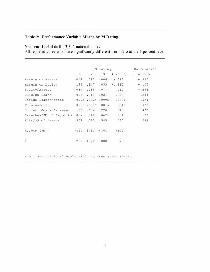
M ratings vary with financial performance in the expected direction, and all of the

reported correlation coefficients in Table 2 are significantly different from zero at the 1

percent level. M ratings improve as profitability (ROA, ROE) and as capital levels

(equity/assets) increase, and get worse as asset quality (OREO/real estate loans) deteriorates.

The percentage of loans made to executive officers in M 4- or 5-rated banks is triple the

percentage of insider loans in M 1-rated banks, evidence that the M rating may contain

information about principal-agent problems. Fee income as a percentage of assets is

negatively related to M, suggesting that highly rated managers moved their banks quickly into

nontraditional products and services.

M ratings are positively related to the efficiency ratio (noninterest costs/revenue).

Furthermore, the evidence indicates sizeable technical inefficiencies in poorly run banks – M

4- or 5-rated banks employed one-third more workers per asset dollar, and operated two-thirds

more branches per deposit dollar, than did M 1-rated banks.

M ratings tended to get worse as banks got smaller. The average M 4- or 5-rated8

bank ($320 million in assets) was about three-quarters the size of the average M 1-rated bank

($441 million). Given that national banks range in assets from less than $10 million to over

$1 billion, however, it is unlikely that bank size is the major determinant of the other results

shown in Table 2.

14

____________________________________________________________________

Table 2: Performance Variable Means by M Rating

Year-end 1991 data for 3,345 national banks. All reported correlations are significantly different from zero at the 1 percent level.____________________________________________________________________

M Rating Correlation

1 2 3 4 and 5 with M

Return on Assets .017 .012 .006 -.010 -.445

Return on Equity .198 .147 .053 -1.216 -.106

Equity/Assets .089 .085 .078 .060 -.254

OREO/RE Loans .005 .011 .021 .040 .284

Inside Loans/Assets .0003 .0004 .0005 .0008 .074

Fees/Assets .0032 .0019 .0016 .0010 -.073

Nonint. Costs/Revenues .622 .684 .770 .918 .402

Branches/$M of Deposits .037 .042 .047 .054 .133

FTEs/$M of Assets .507 .527 .585 .680 .244

Assets ($M) $441 $411 $364 $320*

N 289 1970 808 278

* OCC multinational banks excluded from asset means.

____________________________________________________________________

Banks with M ratings of 4 were included in the poorly managed sample because there were too few national banks9

with M ratings of 5 to estimate a cost frontier. See section IV for a description of this data.

m The factor share equations were generated by differentiating the cost function with respect to W and invoking10

Shepard's lemma. The physical capital share equation was omitted from the estimation to avoid singularity in the

variance-covariance matrix. The remaining four equations were estimated simultaneously using seemingly unrelated

regression (SUR) techniques after imposing the standard symmetry and homogeneity restrictions on the model. See

Johnston (1984), pp. 335-336. See DeYoung (1993) for a discussion of the choice of specification and functional

form.

15

III. Measuring X-Inefficiency

Assuming that M ratings are valid measures of management quality in commercial

banks, the results in Table 2 suggest that poorly managed banks are more X-inefficient than

well-managed banks. The cost differences revealed in Table 2, however, are not controlled

for interbank differences in product mix, input prices, organizational form, or branching laws

that can affect costs. This section develops a statistical model to estimate the difference in X-

inefficiency between banks with M ratings of 1 ("fully effective" management) and banks with

M ratings of 4 or 5 ("generally inferior" or "incompetent" management) while controlling for

these conditions.9

III.A Cost Model

Following Berger and Humphrey (1991), a pair of thick cost frontiers were generated

by estimating the following multiproduct translog cost model separately for well-managed and

poorly managed banks:10

16

where:

C = interest expense plus noninterest expense.

iY = output vector, i = 1,5 (commercial and industrial loans, real estate loans, consumer loans, securities, and transactions deposits)

mW = input price vector, m = 1,4 (wage rate, price of physical capital, interest rate paid for deposited funds, interest rate paid on purchased funds)

LIMIT = dummy equal to 1 in limited branching states.UNIT = dummy equal to 1 in unit banking states.BHC = dummy equal to 1 if bank is a member of a bank holding company.

mS = the share of C generated by expenditures on input m.,,0 = error terms assumed to capture random cost fluctuations.

The wage rate equals salaries and benefits divided by FTE labor; the price of physical

capital equals depreciation expense divided by the original price of physical assets; the price of

deposited funds equals interest expense on transactions, savings, and time deposits (excluding

CDs > $100,000) divided by these balances; and the price of purchased funds equals interest

expense on large CDs, Fed funds, foreign deposits, and other borrowed funds divided by these

balances. Transactions deposits equal demand deposits, NOW accounts, and other nonsavings

and nontime deposits, and are included as a proxy for the amount of payment and liquidity

services produced by the bank. BHC controls for cost differences due to organizational form.

Berger and Humphrey (1991, p. 121) defend a similar set of assumptions: "...the thick frontier approach may not11

yield precise estimates of the overall level of inefficiencies in banking. However, precise measurement is not our

purpose. Rather, our goals are to get a basic idea of the likely magnitude of inefficiencies..."

17

LIMIT and UNIT are included to control for the impact of branching restrictions on costs.

Two maintained assumptions are necessary to yield the thick frontiers:

A1. The error terms within the well-managed (M1) and the poorly managed (M45) samples

reflect only random chance and luck.

A2. The cost differences between the M1 and M45 samples are not due to random error but

can be divided into two classes of determinants:

a. conditions special to an individual bank or local banking market that are beyond

the short-run control of management (e.g., prices of inputs, mix of demand for

products, organizational form, or branching laws), or

b. conditions that management has the power to reduce or eliminate (e.g., agency

effects or lax cost control when competitive rivalry is not intense) or that are the

result of intrinsic differences in the abilities of managers.

Stated differently, the assumptions imply that M1 banks use a production technology that is

distinctly different from the production technology used by M45 banks, that these technologies

reflect the "quality" (experience, education, native ability, integrity, etc.) of bank

management, and that managers can influence costs only through the amount and combination

of inputs they hire. These assumptions obviously do not hold exactly, but they are reasonable

approximations for the purpose at hand. 11

Although the number of branches operated by a bank has been shown elsewhere to be a

significant determinant of costs, no branch variable is included in the cost function.

18

According to our maintained assumptions, differences in the regressors between the upper and

lower frontiers are due to exogenous factors beyond the control of the bank and hence do not

reflect efficiency, while differences in the parameters between the upper and lower frontiers

do reflect differences in efficiency. The regressors in equation (1) – output mix, input prices,

branching laws, and holding company organization – are all arguably beyond the short-run

control of bank management (see section III.B), but management clearly has the short-run

ability to close existing branches or (within limits in some states) open new branches. Hence,

branches were excluded from the cost function, and their effect on costs is contained in the

regression residual.

III.B. Estimating Cost Inefficiency Associated with Management Quality

The predicted percent difference in unit costs between banks in the M45 and M1 cost

frontiers is given by:

p,m p m mwhere estimated unit costs AC = C (X )/A and:

pC (.) = predicted total costs using the estimated parameters from equation (1) when the model is estimated for banks in sample p, p = (M1,M45).

mX = the vector of variable means for banks in sample m, m = (M1,M45).

mA = the average assets held by banks in sample m, m = (M1,M45).

Thus, DIFFM is the percentage by which the predicted unit cost of a poorly managed bank

exceeds, on average, the predicted unit costs of a well-managed bank, where well-managed

and poorly managed are defined by examiners' M ratings.

By construction, the cost discrepancies captured in DIFFM can be traced to two

19

differences between the estimated M45 and M1 cost frontiers: differences in the estimated

equation (1) parameters, or differences in the mean values of the regressors used to evaluate

equation (1). Differences in the parameters between the M45 and M1 frontiers are attributed

to the different production technologies being used by the banks – and hence, attributed to

differences in decisions made by managers – in the two samples. In contrast, differences in

the mean values of the regressors between the M45 and M1 cost frontiers are attributed to

exogenous factors beyond the control of banks, such as local market conditions (input prices,

state branching laws), customer demand (output level, output mix), or conditions that

managers cannot alter in the short-run (organizational form). Thus, the portion of DIFFM

owing to these exogenous factors is given by:

M1,M45where AC is the estimated unit cost for a bank operating with the estimated parameters of

the average M 1-rated bank, but which receives exogenously the market conditions faced by

the average M 4- or M 5-rated bank. The predicted percentage difference in unit costs

between well-managed and poorly managed banks that cannot be attributed to exogenous

market conditions is given by:

INEFFM is the percentage by which the predicted unit cost of the average poorly managed

bank exceeds the predicted unit costs of the average well-managed bank, after controlling for

the impact of exogenous factors on cost. It approximates the X-inefficiency in commercial

It is possible that bank examiners make systematic (in addition to random) errors which result in higher M ratings12

for banks that face exogenous, cost-increasing conditions. This issue is beyond the scope of this paper.

20

banks due to differences in management quality.

MARKETM is expected to be small, but positive. Assuming that bank examiners

control adequately for market conditions, the M ratings they assign will be unrelated to

conditions beyond the control of bank managers, and MARKETM will be zero. However,12

the maintained assumption that the exogenous variables are beyond the short-run control of

management does not hold perfectly. For example, input prices could be related to

management quality if poorly managed banks reprice their deposits less often than well-

managed banks reprice theirs. This X-inefficiency will be captured in MARKETM.

III.C Management-Related X-Inefficiency as a Percentage of Total X-Inefficiency

INEFFM can be compared to estimates of total (management-related plus

nonmanagement-related) X-inefficiency to approximate the portion of X-inefficiency in banks

associated with differences in management quality. Again following Berger and Humphrey

(1991), the following sampling technique was used to select high-cost and low-cost banks from

the population of national banks in 1991. The population of banks was placed in order by

asset size, and then partitioned into deciles. Within each asset decile, banks were ordered by

average cost (the sum of interest and noninterest costs as a percentage of assets) and then

partitioned into quartiles. The lowest cost quartiles from each of the asset deciles were

assumed to contain the most cost-efficient or "best practices" banks; this subset of banks is

denoted Q1. Similarly, the highest-average-cost quartiles were assumed to contain the most

21

cost-inefficient banks; this subset of banks is denoted Q4.

Thick frontier cost functions were estimated using cost model (1) and (2) for both the

cost-efficient and the cost-inefficient samples. The maintained assumptions presented above

about the error terms continue to hold. The estimation results were used to generate a

corollary to INEFFM:

INEFFQ is the predicted percentage difference in unit costs between the most cost-efficient

banks and most cost-inefficient banks, after controlling for market factors. A priori, one

would expect the cost residual INEFFQ to be larger than the cost residual INEFFM, because

samples Q1 and Q4 are determined directly by costs, whereas samples M1 and M45 are

determined based on a phenomenon (M ratings) that is merely related to costs.

IV. Data

There were 3,345 national banks for which complete end-of-year 1991 data were

available. Thus, to determine the Q1 and Q4 subsamples, there were 335 banks in each asset

decile (3,345÷ 10), 84 banks in each quartile within these asset deciles (335÷ 4), and 840

banks in the upper and lower unit cost quartiles (84*10). Table 3a contains descriptive

statistics for Q1 and Q4 banks.

Descriptive statistics for M1 and M45 banks are shown in Table 3b. Of the 3,345

national banks in the overall sample, there were 289 banks in the M1 subsample and 278

banks in the M45 subsamples. A rating of M= 1 is "indicative of management that is fully

22

____________________________________________________________________

Table 3a: Descriptive Statistics for Upper and Lower Cost Quartile Banks

Year-end 1991 data for 1,681 national banks. OCC multinational banks excluded.Dollar amounts in thousands.____________________________________________________________________

lower quartile upper quartile % of % of assets assets

Assets $418,610 $440,076

Cost 22,815 5.45% 33,215 7.55% C&I Loans 64,295 15.35% 73,976 16.81%Consumer Loans 45,874 10.96% 59,322 13.48%RE Loans 85,808 20.50% 125,484 28.51%Securities 98,001 23.41% 75,188 17.09%Transactions Dep. 97,852 23.38% 99,274 22.56%

lower quartile upper quartile

Wage ($1,000/FTE) $28.415 $30.817

Rate paid on: Deposited Funds 4.29% 5.08% Purchased Funds 6.51% 7.66% Physical Capital 43.50% 56.72%

BHC Dummy 0.763 0.723Unit Dummy 0.112 0.022Limit Dummy 0.351 0.289

M Rating 2.126 2.753

____________________________________________________________________

23

____________________________________________________________________

Table 3b: Descriptive Statistics for M = 1 and M = 4 or 5 Banks

Year-end 1991 data for 567 national banks. OCC multinational banks excluded.Dollar amounts in thousands.____________________________________________________________________

M = 1 banks M = 4,5 banks % of % of assets assets

Assets $441,116 $320,413

Cost 27,798 6.30% 24,051 7.51% C&I Loans 69,596 15.78% 54,636 17.05%Consumer Loans 80,912 18.34% 25,404 7.93%RE Loans 91,130 20.66% 111,275 34.73%Securities 93,385 21.17% 52,715 16.45%Transactions Dep. 94,804 21.49% 76,442 23.86%

lower quartile upper quartile

Wage ($1,000/FTE) $28.613 $30.439

Rate paid on: Deposited Funds 4.84% 4.85% Purchased Funds 6.65% 7.56% Physical Capital 38.97% 53.84%

BHC Dummy 0.889 0.612Unit Dummy 0.045 0.033Limit Dummy 0.467 0.207

M Rating 1.000 4.225

N 289 276____________________________________________________________________

24

effective," a rating of M= 4 is "indicative of a management that is generally inferior in

ability," and a rating of M= 5 is assigned to "institutions where incompetence has been

demonstrated." M 4-rated banks were added to M 5-rated banks to form the subsample of

"poorly managed" banks because only 62 banks had M ratings of 5.

All variables used in the cost model were constructed from end-of-year 1991 data from

the Reports of Condition and Income (call report), except for LIMIT and UNIT, which were

constructed using information from Amel (1991). All CAMEL ratings were read from the

National Bank Surveillance Video Display System (NBSVDS) and are used with the

permission of the Office of the Comptroller of the Currency.

V. Results

Estimates of overall X-inefficiency (DIFFQ, MARKETQ, INEFFQ) are reported in

Table 4, and estimates of management-related X-inefficiency (DIFFM, MARKETM,

INEFFM) are reported in Table 5. In both tables, the results are segregated into asset classes

to reveal possible relationships between size and X-inefficiency. (Parameter estimates for the

Q1, Q4, M1, and M45 cost frontiers are reported in the Appendix.)

The estimates of overall X-inefficiency are consistent with those found in other studies of

commercial banks. INEFFQ (overall X-inefficiency after adjusting for exogenous influences)

averaged about 19 percent and ranged between 15 and 38 percent. Contrary to the hypothesis

that larger banks are able to operate closer to the cost frontier, INEFFQ increases as banks get

larger. In contrast, MARKETQ (X-inefficiency attributable to exogenous conditions)

25

____________________________________________________________________

Table 4: Total Cost Inefficiency

Year-end 1991 data for upper quartile and lower quartile national banks. AC = predicted total costs as a percentage of total assets.Assets in millions of dollars. ____________________________________________________________________

lower quart. upper quart. Assets N AC N AC DIFFQ MARKETQ INEFFQ

$ 0-25 123 .057 114 .077 34.2% 17.7% 16.5% 25-50 187 .057 198 .078 37.7% 21.6% 16.0% 50-100 215 .056 208 .076 35.7% 17.4% 18.3% 100-300 202 .054 206 .072 33.3% 13.5% 19.8% 300-500 35 .055 33 .071 28.2% 12.9% 15.4% 500-1,000 27 .050 26 .069 37.2% 1.6% 35.7%1,000+ 51 .044 56 .058 29.1% -4.5% 33.6%

Total 840 841

Mean 34.8% 15.5% 19.3%

____________________________________________________________________

26

________________________________________________________________________

Table 5: Management-Related Cost Inefficiency

Year-end 1991 data for selected national banks. Assets in millions of dollars. AC = predicted total costs as a percentage of total assets.________________________________________________________________________

M = 1 M = 4,5 INEFFM÷

Assets N AC N AC DIFFM MARKETM INEFFM INEFFQ

$ 0-25 23 .058 83 .072 23.5% 5.8% 17.7% 107.5% 25-50 42 .063 81 .076 20.8% 11.6% 9.1% 57.1% 50-100 80 .063 45 .073 15.9% 5.1% 10.8% 59.0% 100-300 90 .062 40 .071 14.5% 3.6% 10.9% 55.1% 300-500 24 .062 10 .068 9.9% 3.5% 6.4% 41.6% 500-1,000 16 .062 2 .067 8.5% -11.4% 19.9% 55.8%1,000+ 14 .049 17 .054 12.2% -3.1% 15.3% 45.5%

Total 289 278

Mean 16.7% 4.6% 12.1% 65.4% ________________________________________________________________________

Berger and Humphrey (1991) found that MARKET explained about 7 percent of DIFF for banks in unit banking13

states in 1984, and about 13 percent of DIFF for banks in branch banking states in the same year. Pantalone and

Platt (1993) found that MARKET explained 28 percent of DIFF for thrifts in 1978 and 33 percent of DIFF for thrifts

in 1988.

Both UNIT and LIMIT had significant negative coefficients in the Q1 cost frontier, suggesting that banks that can14

branch freely tend to overbranch. Hence, MARKETQ will be larger to the extent that Q4 banks are more likely than

Q1 banks to operate in states without branching restrictions. The data in Table 3a shows that both UNIT (.021 vs.

.112) and LIMIT (.288 vs. .351) were lower for Q4 banks.

27

comprised about 45 percent of DIFFQ (unadjusted X-inefficiency), a larger portion than found

in other thick frontier cost studies. This may be due to differences in the way the cost model13

is constructed – among other differences, earlier studies have specified separate equations for

operating costs and interest costs, included variables to measure the number of branch offices,

and estimated the model separately for banks in branching and unit banking states. 14

Banks judged by examiners to be poorly managed displayed substantial X-inefficiency

relative to banks judged by examiners to be well-managed. INEFFM (management-related X-

inefficiency after adjusting for conditions beyond the control of management) averaged about

12 percent and ranged between 6 percent and 20 percent. However, the cost residual between

M1 and M45 banks was uniformly smaller than the cost residual between Q1 and Q4 banks.

Overall, INEFFM averaged about 65 percent the size of INEFFQ. As expected, MARKETM

was relatively small, averaging 4.6 percent, or about 28 percent of the total cost residual

DIFFM. There appears to be no relationship between management-related X-inefficiency and

bank size.

In Section II, M ratings were shown to be positively related to financial performance,

and it was suggested that bank examiners might not assess management quality independently

from the other performance ratings. If so, then the portion of X-inefficiency associated with

For the well-managed banks, mean CAMEL=2.12, mean actual M=1.66, and mean predicted M=2.68. For the15

poorly managed banks, mean CAMEL=2.62, mean actual M = 3.33, and mean predicted M = 2.28.

A similar procedure based on the highest and lowest residuals from the OLS model produced results (not shown)16

substantially the same as those in Table 6.

28

management quality may be less than 28 percent of banking costs, and differences in

management quality might account for less than 65 percent of total X-inefficiency in banks.

To address this concern, the results of the ordered logit model presented in Section II were

used to separate the M rating into two components: information coincident with that portion

of a bank' s financial performance represented by the C, A, E, and L ratings, and information

that is orthogonal to these four performance ratings. Each bank' s actual M rating was

compared to the M rating predicted for it (i.e., the M category assigned the highest probability

estimate) by the logit model. A bank was assumed to be well-managed if its actual M rating

was better than its predicted M rating, and poorly managed if its actual M rating was worse

than its predicted M rating. This procedure resulted in 515 well-managed banks and 558

poorly managed banks. Thick cost frontiers were estimated for these two sets of banks, and15

versions of DIFF, MARKET, and INEFF were generated.

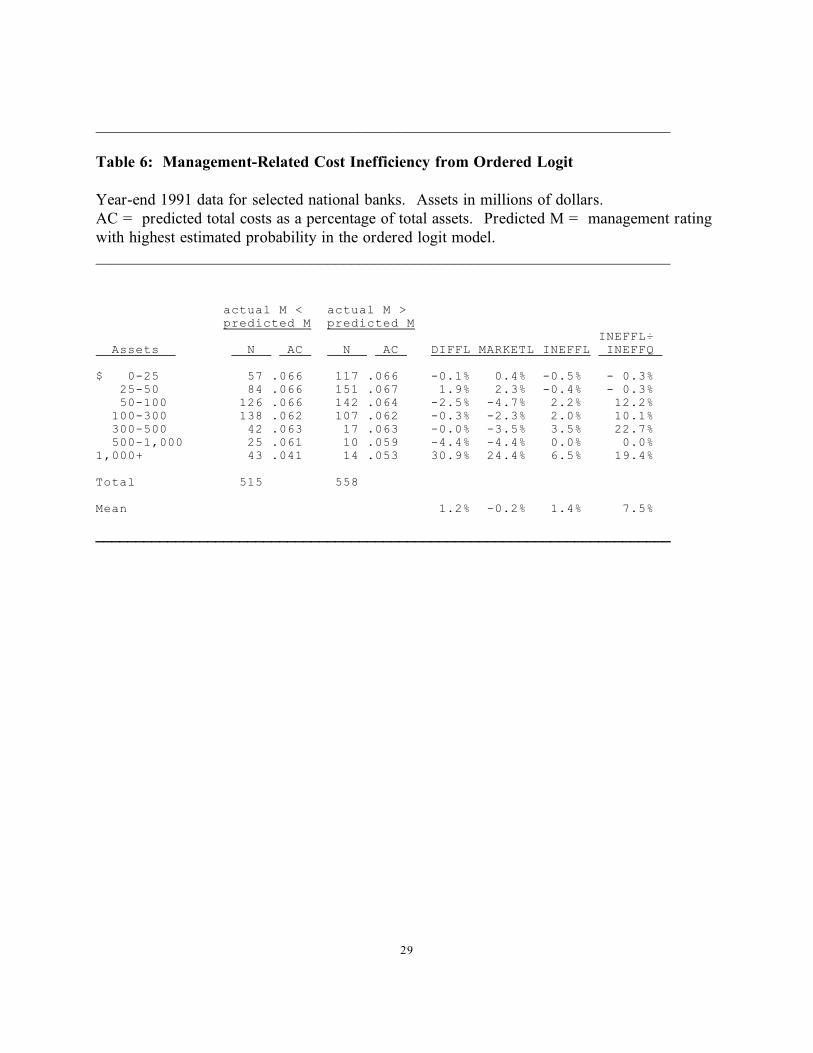
The results are reported in Table 6. On average, the X-inefficiency (INEFFL)16

associated with this "pure" measure of management quality increased costs by only about 1½

percent, and equaled only about 7 percent of total X-inefficiency (INEFFQ). There are two

basic ways to interpret these results. At one extreme, one could conclude that management

quality plays only a small role in determining cost differences between banks. At the other

extreme, one could conclude that management quality plays a large role in determining inter-

bank cost differences, but that roughly 90 percent of its impact (7 percent ÷ 65 percent) is

29

________________________________________________________________________

Table 6: Management-Related Cost Inefficiency from Ordered Logit

Year-end 1991 data for selected national banks. Assets in millions of dollars. AC = predicted total costs as a percentage of total assets. Predicted M = management ratingwith highest estimated probability in the ordered logit model.________________________________________________________________________

actual M < actual M > predicted M predicted M

INEFFL÷ Assets N AC N AC DIFFL MARKETL INEFFL INEFFQ

$ 0-25 57 .066 117 .066 -0.1% 0.4% -0.5% - 0.3% 25-50 84 .066 151 .067 1.9% 2.3% -0.4% - 0.3% 50-100 126 .066 142 .064 -2.5% -4.7% 2.2% 12.2% 100-300 138 .062 107 .062 -0.3% -2.3% 2.0% 10.1% 300-500 42 .063 17 .063 -0.0% -3.5% 3.5% 22.7% 500-1,000 25 .061 10 .059 -4.4% -4.4% 0.0% 0.0%1,000+ 43 .041 14 .053 30.9% 24.4% 6.5% 19.4%

Total 515 558

Mean 1.2% -0.2% 1.4% 7.5% ________________________________________________________________________

30

reflected in measurable financial performance captured by examiners in the C, A, E, and L

ratings (e.g., good underwriting standards that result in fewer costly nonperforming loans, or cost

controls that result in higher operating margins), while the other 10 percent of its impact is

associated with less tangible financial outcomes (e.g., good internal controls that result in lower

agency costs).

VI. Conclusions

It seems a straightforward proposition that good managers will run their banks efficiently

and bad managers will run their banks inefficiently. The results found here for national banks in

1991 confirm this common sense proposition. After adjusting for exogenous factors beyond the

control of management, unit costs at national banks with "inferior" or "incompetent"

management (according to bank examiners) averaged about 12 percent higher than unit costs at

banks with "fully effective" management. This difference amounts for roughly two-thirds of total

banking X-inefficiency found both here and in other studies. This suggests that a large portion of

the cost inefficiencies present in commercial banks is associated with – though perhaps not

caused by – the quality of the managers that run those banks. When the 12 percent figure was

disaggregated, about 90 percent was attributed to differences in management quality associated

with subpar financial performance (e.g., poor asset quality or low earnings) and the remaining 10

percent was attributed to differences in management quality not reflected by financial

performance (e.g., poor internal controls that might foster principal-agent problems).

Some caution should be exercised in interpreting these results, which rest on several

assumptions about the characteristics of error terms in the statistical model, as well as on the

See Berger, Hunter, and Timme (1993) for a discussion of this literature.17

31

assumption that M ratings sufficiently capture interbank differences in management quality.

Although no good substitute measure of management quality exists, techniques that make

different assumptions about the error terms are available (e.g., stochastic frontier or data

envelopment), and might be used to test the robustness of the results found here.

Finally, the results found here suggest that an active market for corporate control of

banks, which supposedly identifies bad managers and replaces them with better managers, would

be a potent weapon for reducing X-inefficiency. The empirical literature on bank mergers,

however, raises doubts about the efficiency-enhancing potential of bank mergers. Although

some studies of bank mergers have found post-merger improvements in stock prices, earnings,

loan-to-asset ratios, and labor expenses, the existing literature contains little evidence of post-

merger improvement in X-inefficiency. Future research might attempt to reconcile the results17

of these studies.

32

References

Aly, Hasan, Richard Grabowski, Carl Pasurka, and Nanda Rangan. "Technical, Scale, and

Allocative Efficiencies in U.S. Banking: An Empirical Investigation." The Review of

Economics and Statistics, 72: 211-219 (1990).

Amel, Dean. "State Laws Affecting Commercial Bank Branching, Multibank Holding Company

Expansion, and Interstate Banking." Unpublished paper (1991).

Bauer, Paul, Allen Berger, and David Humphrey. "Efficiency and Productivity Growth in U.S.

Banking." In H.O. Fried, C.A.K. Lovell, and S.S. Schmidt, eds., The Measurement of

Productive Efficiency: Techniques and Applications, Oxford: Oxford University Press

(1993).

Berger, Allen, Diana Hancock, and David Humphrey. "Bank Efficiency Derived from the Profit

Function." Journal of Banking and Finance, 17: 317-347 (1993).

Berger, Allen, and David Humphrey. "The Dominance of Inefficiencies over Scale and Product

Mix Economies in Banking." Journal of Monetary Economics, August: 117-148 (1991).

Berger, Allen, and David Humphrey. "Megamergers in Banking and the Use of Cost Efficiency

as an Antitrust Defense." The Antitrust Bulletin, 37: 541-600 (1992).

Berger, Allen, William Hunter, and Stephen Timme. "The Efficiency of Financial Institutions:

A Review and Preview of Research Past, Present, and Future." Journal of Banking and

Finance, 17: 221-249 (1993).

33

DeYoung, Robert. "Determinants of Cost Efficiencies in Bank Mergers." Office of the

Comptroller of the Currency, Economic & Policy Analysis Working Paper 93-1.

Washington, DC (1993).

Elyasiani, Elyas, and Seyed Mehdian. "A Nonparametric Approach to Measurement of

Efficiency and Technological Change: The Case of Large U.S. Commercial Banks."

Journal of Financial Services Research, 4: 157-168 (1990).

Evanoff, Douglas, and Philip Israilevich. "Productive Efficiency in Banking." Federal Reserve

Bank of Chicago, Economic Perspectives, July: 11-32 (1991a).

Evanoff, Douglas, and Philip Israilevich. "Regional Differences in Bank Efficiency and

Technology." The Annals of Regional Science, 25: 41-54 (1991b).

Evanoff, Douglas, Philip Israilevich, and Randall Merris. "Relative Price Efficiency, Technical

Change, and Scale Economies for Large Commercial Banks." Journal of Regulatory

Economics, 2: 281-298 (1990).

Federal Financial Institutions Examination Council. Reports of Condition and Income (call

reports). Washington, DC (1991).

Ferrier, Gary, and C.A. Knox Lovell. "Measuring Cost Efficiency in Banking: Econometric

and Linear Programming Evidence." Journal of Econometrics, 46: 229-245 (1990).

Grabowski, Richard, Nanda Rangan, and Rasoul Rezvanian. "Organizational Forms in Banking:

An Empirical Investigation of Cost Efficiency." Journal of Banking and Finance, 17:

531-538 (1993).

Johnston, J. Econometric Methods, 3rd ed., New York: McGraw Hill (1984).

34

Leibenstein, Harvey. "Allocative Efficiency vs. X-Efficiency." American Economic Review,

56: 392-415 (1966).

Maddala, G.S. Limited-Dependent and Qualitative Variables in Econometrics. Cambridge:

Cambridge University Press (1983).

Newman, Joseph, and Ronald Shrieves. "Multibank Holding Company Effect on Cost

Efficiency in Banking." Journal of Banking and Finance, 17: 709-732 (1993).

Office of the Comptroller of the Currency. "Uniform Financial Institutions Rating System,"

Examining Circular 159. Washington, DC (1979).

Office of the Comptroller of the Currency. Bank Failure: An Evaluation of the Factors

Contributing to the Failure of National Banks. Washington, DC (1988).

Office of the Comptroller of the Currency. National Bank Surveillance Video Display

System. Washington, DC (1991, 1992).

Pantalone, Coleen, and Marjorie Platt. "The Effects of Acquisition and Deregulation on Thrift

Cost Inefficiencies: A Thick Frontier Approach." Unpublished conference paper.

Indianapolis: Midwest Finance Association Meetings (1993).

Pi, Lynn, and Stephen Timme. "Corporate Control and Bank Efficiency." Journal of Banking

and Finance, 17: 515-530 (1993).

35

Appendix

Equation 1 parameter estimates for Q1, Q4, M1, and M45 samples.

0 1 2 3 4 5 " " " " " " Q1 4.40828* -0.22839 0.54268* 0.51123* -0.00522 -0.10510 Q4 3.59959* -0.53617* 0.38666* -0.06678 0.31591* 0.49178*M1 4.28801 0.42704 -0.20161 0.20593 -0.64860* 1.07170*M45 1.83230 -0.09688 0.18903 -0.03932 -0.05907 0.52832

11 22 33 44 55 12 $ $ $ $ $ $Q1 0.065516* 0.02812* 0.09727* 0.11592* 0.14083* -0.02441*Q4 0.031516* 0.05541* 0.20275* 0.09241* 0.08866* -0.02708*M1 0.047351* 0.08056* 0.13685* 0.09322* 0.12620* -0.02555 M45 0.097173* 0.04369* 0.16195* 0.09774* 0.16431* -0.02912*

13 15 23 24 $ 14 $ $ $ 25 $ $Q1 -0.02671* 0.00482 -0.01789 0.00542 -0.02870* 0.02003Q4 -0.02091* -0.00412 0.02577* -0.01058* -0.03359* 0.02080*M1 -0.02382* -0.02844 0.02595 -0.00773 -0.01259 -0.01032M45 -0.02281 -0.00400 0.03597 0.01627 -0.01536 -0.02011

34 35 45 1 2 3 $ $ $ ( ( (Q1 -0.01513* -0.05183* -0.07208* -0.59212* 0.51480* 0.75634*Q4 -0.02966* -0.13151* -0.01327 0.03623 2.15105* -0.74878*M1 0.01691 -0.11361* -0.05043* -0.61779 2.31158* -0.92748M45 -0.04195* -0.09108* -0.02433 0.72170 1.31255* -0.80376

5 22 33 44 12 ( 11 * * * **Q1 0.32097* 0.14883* 0.06987 0.07141* -0.00385 0.02142Q4 -0.43850* -0.00179 0.30252* 0.02773 0.03397* -0.10461*M1 0.23369 0.16329 0.42065* 0.04218 0.01857 -0.22455*M45 -0.23049 -0.13777 0.16800 -0.20137* -0.00705 -0.03845

13 14 23 24 34 11 * * * * * 2Q1 -0.13713* -0.03312 -0.09526 0.02702 0.00995 0.06126*Q4 0.05729 0.04910 0.05576* -0.09331* 0.01023 0.10958*Q1 0.14302 -0.08177 -0.21995* 0.02844 0.03475 -0.03616M45 0.13326 0.04295 0.05520 -0.09111* 0.05520 0.03706

12 13 14 21 22 23 2 2 2 2 2 2Q1 -0.06769* 0.02700 -0.02068* -0.06556* 0.11439* -0.03880*Q4 -0.05128* -0.02080 -0.03748* -0.05847* 0.05658* -0.04354*M1 0.03073 0.00875 -0.00333 0.00604 -0.05927 0.03963 M45 -0.04591 0.00600 0.00274 -0.01413 -0.05815 0.06248

34 31 32 33 34 41 2 2 2 2 2 2

Q1 -0.01003 -0.07186* 0.04111 0.013074 0.01766* 0.02951Q4 0.04542* 0.01723 -0.05603* 0.022597 0.01619 -0.05344*M1 0.01359 -0.01442 0.02370 0.001571 -0.01086 0.10388*M45 0.00980 0.00564 -0.02287 -0.016810 0.03403* 0.01978

( * indicates statistical significance at the 10 percent level.)

Appendix

Continued.

42 43 44 51 52 54 2 2 2 2 2 2Q1 -0.01151 0.01072 -0.02873* 0.03268 -0.06448 0.00261Q4 -0.01695 0.05048* 0.01990* 0.00118 0.00325 0.02957M1 -0.04401 -0.03227 -0.02760 -0.08696 0.04018 -0.00998

36

M45 -0.01830 0.01310 -0.01459 -0.02755 0.11351 -0.04927

54 BHC UNIT LIMIT 2 8 8 8 R 2

Q1 0.02918* -0.00628 -0.03526* -0.00900 0.9891Q4 -0.03401* 0.02548* -0.03790 0.00300 0.9909M1 0.05676 0.05133* -0.02776 -0.01655 0.9930M45 -0.03669 0.02316 -0.08143 0.01137* 0.9917

( * indicates statistical significance at the 10 percent level.)