Embed Size (px)
Citation preview

Int. J. of Systems, Control and Communications, Vol. x, No. x, xxxx 1
Witsenhausen’s counterexample as
Assisted Interference Suppression
Pulkit Grover and Anant Sahai
Wireless Foundations, Department of EECSUniversity of California at Berkeley, CA-94720, USA{pulkit, sahai}@eecs.berkeley.edu
Abstract: Despite the seemingly irreducible simplicity of Witsenhausen’scounterexample, the optimal control law for the problem is as yet un-known. It has been observed that the problem contains an implicitcommunication channel, which motivates formulating a vector versionof the Witsenhausen counterexample that simplifies the problem in thelimit of large vector lengths. This vector version can be viewed as a toywireless communication problem that we call “Assisted Interference Sup-pression” and is conceptually related to the “cognitive radio channel”studied in information theory. A new information-theoretic lower boundon the average costs for this problem is derived. Then, using conceptsof lossy compression, channel coding, and dirty-paper coding, nonlin-ear control strategies are developed that attain costs within a uniformlybounded constant factor of the optimal cost for this vector problem inthe limit of infinite vector length. This is demonstrated by showing thatthe ratio of the upper and lower bounds is no more than 2 regardless ofthe problem parameters. Restricted to the scalar problem, it is shownthat the new lower bound can be better than Witsenhausen’s bound byan arbitrarily large factor.
Keywords: Witsenhausen’s counterexample, distributed control, in-formation theory
Reference to this paper should be made as follows: Pulkit Grover andAnant Sahai (2009) ‘Witsenhausen’s counterexample as Assisted Inter-ference Suppression’, Int. J. Journal of Systems, Control and Commu-nications, Vol. x, No. x, pp.xxx–xxx.
Biographical notes: Pulkit Grover (BS ’03, IIT Kanpur, MS ’05, IITKanpur) is a graduate student at the Department of Electrical Engineer-ing and Computer Sciences at the University of California at Berkeleysince 2005. He is a member of the Wireless Foundations center. Hisresearch interests are in information theory, computational complexity,distributed control, spectrum sharing and finance.
Anant Sahai (BS ’94 UCB, MS ’96 MIT, PhD ’01 MIT) joined the De-partment of Electrical Engineering and Computer Sciences at the Uni-versity of California at Berkeley in 2002 as an Assistant Professor. Heis a member of the Berkeley Wireless Research Center and the Wire-less Foundations center. His research interests are in wireless commu-nication, spectrum sharing, signal processing, information theory, anddistributed control. He is particularly interested in bridging the gulfbetween information theory and distributed control.
Copyright c© 200x Inderscience Enterprises Ltd.

2 Pulkit Grover and Anant Sahai
1 Introduction
Distributed control problems have proved challenging for control engineers. In1968, Witsenhausen (Witsenhausen, 1968) gave a counterexample showing thateven a seemingly simple distributed control problem can be hard to solve. For thecounterexample, Witsenhausen chose a two-stage distributed LQG system. Thechoice is appropriate because LQG systems that are not distributed are well un-derstood — control laws linear in the observations are optimal for such systems.For his counterexample, Witsenhausen provided a nonlinear control strategy thatoutperforms all linear laws, thus arguing that distributed systems might be harderto understand. It is now clear that Witsenhausen’s problem itself is quite hard;the optimal strategy and the optimal costs for the problem are still unknown. Thenon-convexity of the problem makes the search for an optimal strategy hard (Bansaland Basar, 1987; Baglietto et al., 1997; Lee et al., 2001). Discrete approximationsof the problem (Ho and Chang, 1980) are even NP-complete (Papadimitriou andTsitsiklis, 1986).
In order to understand what makes the problem hard, modifications of theproblem have been considered that still admit linear optimal solutions. In (Bansaland Basar, 1987), for example, Bansal and Basar consider a parametrized familyof two-stage stochastic control problems. The family includes the Witsenhausencounterexample. Using results from information theory, the authors show that forthis family, whenever the cost function does not contain a product of two decisionvariables, affine control laws are still optimal. In (Rotkowitz, 2006), Rotkowitzshows that affine control laws continue to be optimal for a deterministic variant ofthe counterexample if the cost function is the induced two-norm instead of Witsen-hausen’s original expected two-norm.
Ho, Kastner, and Wong (Ho et al., 1978) view the Witsenhausen problem asa close sibling of Shannon’s problem of explicit communication. Mitter and Sa-hai (Mitter and Sahai, 1999) build upon this observation to suggest that the coun-terexample might be hard because there is an implicit communication channel fromthe first controller to the second. The first stage cost can be interpreted as the powerthat is input to this channel. The second stage cost is the distortion in estimatingthe state at time 1. Using this interpretation, they propose nonlinear control strate-gies based on state quantization. Over a range of possible problem parameters andcorresponding quantization levels, these nonlinear strategies can outperform opti-mal linear strategies by an arbitrarily large factor. Martins (Martins, 2006) pointsout that even in the presence of a non-perfect (but still pretty good) explicit com-munication link, nonlinear strategies continue to outperform linear ones.
In this paper, we ask the following question: Can the problem actually be simpli-fied by using the observation that it has an implicit communication channel (Mitterand Sahai, 1999)? Experience from information theory suggests that it is often eas-ier to analyze communication problems with asymptotically long vector lengths, be-cause they allow us to avoid the complications of the geometry of finite-dimensionalspaces. The asymptotically-long vector length setting also permits the use of the
Witsenhausen’s counterexample as assisted interference suppression 3
laws of large numbers. However, as pointed outa by Tatikonda (Tatikonda, 2000),in control problems such limits need to be interpreted as wide-area spatial asymp-totics rather than the long-delay interpretation favored in communications theory.This motivates us to propose a vector version of the counterexample in Section 2that is illustrated in Fig. 1(a). Section 3 interprets the vector problem as an infor-mation theory problem, shown in Fig. 1(b) where the distributed controllers C1 and
C2 are interpreted as an encoder and a decoder. Section 3.1 provides a toy wire-
less communication problem, called Assisted Interference Suppression, that can bemodeled by the vector Witsenhausen counterexample. Section 3.2 shows that theproblem is one of many closely related information theory problems, some of whichhave been recently addressed in the literature (Costa, 1983; Merhav and Shamai,2007; Kim et al., 2008).
From a control perspective, our claim that the vector formulation simplifiesthe problem is counterintuitive because it might seem that the simplest versionof the problem must contain the fewest number of variablesb. In Section 4 weshow that the asymptotic vector extension is indeed easier to understand since itpermits us to characterize the optimal costs within a constant factor. This con-stant factor is uniformly bounded over all values of the problem parameters k andσ2
0 . This characterization is performed in three steps. First, a new information-theoretic lower bound to the cost is derived. Random-coding based upper boundsare then provided on the cost by analyzing nonlinear control strategies inspiredby the information-theoretic techniques of lossy source coding, channel coding anddirty-paper coding (Costa, 1983). Finally, the ratio of the upper bound to the lowerbound is proved to be no greater than 11. Numerical evaluation shows that thisfactor is actually 2 in the worst case, and is close to 1 for most values of the problemparameters. The characterization is in the spirit of some recent advances in infor-mation theory where approximate characterizations of rate-regions within a uniformbound have been obtained for some long standing multiuser problems (Avestimehret al., 2007; Etkin et al., 2007; Avestimehr, 2008).
Section 4.1 also shows that even the scalar restriction of the new lower boundis an improvement over Witsenhausen’s original lower bound for certain parametervalues. Proper selection of parameters shows that the ratio of our lower boundto Witsenhausen’s bound can be arbitrarily large. Because of this looseness inWitsenhausen’s bound, there could not have been analogous results characterizingthe costs for the scalar problem within a constant factor. Whether such a resultis possible for the original scalar problem with the new lower bound is an openquestion, but Section 5 explains why the assumption of asymptotically long vectorlengths is crucial to the particular results derived here.
aTatikonda used a similar long-vector formulation with parallel dynamics but joint control toshow that the sequential-rate distortion function was indeed the right choice to bound performancein the special case when only the state is penalized (Tatikonda, 2000).
bWitsenhausen himself states “There does not appear to exist any counterexample involvingfewer variables . . . ” than the one presented in (Witsenhausen, 1968).

4 Pulkit Grover and Anant Sahai
(a)
(b)
C
x0
x1 ++
u1 C+
w
1 2u2
x2+
-
E
x0
x1
++u1
D
w
x1^
E[||u1||2] ≤ mP
Figure 1 In (a), the m-length vector version of the Witsenhausen counterexample
is posed as a control problem. The total cost is given by k2
m‖u1‖
2 + 1m‖x2‖
2, and theobjective is to minimize the expected cost. Ci denotes the i−th controller. In (b), the
same problem is cast as an information theory problem, with C1 interpreted as the encoder
E and C2 interpreted as the decoder D. The input u1 to the “channel” has an average
power constraint of P , that is, 1m
Eˆ‖u1‖
2˜≤ P . The objective is to minimize the average
distortion Eˆ‖x1 − bx1‖
2˜. The two problems are equivalent, as shown in Fig. 2.
2 The vector version of Witsenhausen’s counterexample
The scalar Witsenhausen problem is generalized to the vector case, and theresulting block-diagram is shown in Fig. 1(a). The system is still a two-stagecontrol system. The only change from Witsenhausen’s original problem is thatthe states and the inputs are now vectors of length m. A vector is represented inbold font (e.g. x). The space of possible control strategies, including randomizedstrategies, is denoted by S. For expository convenience, we also allow for strategiesthat rely on common randomness shared by the two controllersc. As in conventionalnotation, x is used to denote the state, u the input, and y the observation, and vis used to denote the estimate of any random variable v. The problem descriptionis as follows:
cThe common randomness can be viewed as allowing averaging between different strategies atdifferent times. As we use long vector lengths, such performance can in fact be asymptoticallyattained by cutting the vector into segments and using different strategies on different segments.Thus, all asymptotic results in this paper continue to hold even without the common-randomnessassumption.
Witsenhausen’s counterexample as assisted interference suppression 5
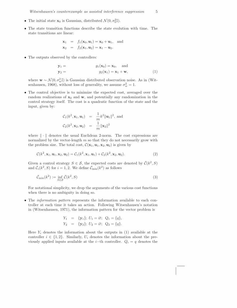
• The initial state x0 is Gaussian, distributed N (0, σ20I).
• The state transition functions describe the state evolution with time. Thestate transitions are linear:
x1 = f1(x0,u1) = x0 + u1, and
x2 = f2(x1,u2) = x1 − u2.
• The outputs observed by the controllers:
y1 = g1(x0) = x0, and
y2 = g2(x1) = x1 + w, (1)
where w ∼ N (0, σ2wI) is Gaussian distributed observation noise. As in (Wit-
senhausen, 1968), without loss of generality, we assume σ2w = 1.
• The control objective is to minimize the expected cost, averaged over therandom realizations of x0 and w, and potentially any randomization in thecontrol strategy itself. The cost is a quadratic function of the state and theinput, given by:
C1(k2,x1,u1) =
1
mk2‖u1‖2, and
C2(k2,x2,u2) =
1
m‖x2‖2
where ‖ · ‖ denotes the usual Euclidean 2-norm. The cost expressions arenormalized by the vector-length m so that they do not necessarily grow withthe problem size. The total cost, C(x1,u1,x2,u2) is given by
C(k2,x1,u1,x2,u2) = C1(k2,x1,u1) + C2(k
2,x2,u2). (2)
Given a control strategy S ∈ S, the expected costs are denoted by C(k2, S)and Ci(k
2, S) for i = 1, 2. We define Cmin(k2) as follows
Cmin(k2) := infS∈S
C(k2, S) (3)
For notational simplicity, we drop the arguments of the various cost functionswhen there is no ambiguity in doing so.
• The information pattern represents the information available to each con-troller at each time it takes an action. Following Witsenhausen’s notationin (Witsenhausen, 1971), the information pattern for the vector problem is
Y1 = {y1}; U1 = ∅; Q1 = {q},Y2 = {y2}; U2 = ∅; Q2 = {q}.
Here Yi denotes the information about the outputs in (1) available at thecontroller i ∈ {1, 2}. Similarly, Ui denotes the information about the pre-viously applied inputs available at the i−th controller. Qi = q denotes the
6 Pulkit Grover and Anant Sahai
randomness available to the two controllers. Here, q is independent of bothx0 and w. Because it is available to both controllers, the allowed strategieshave common randomness.
Note that the second controller does not have knowledge of the output ob-served or the input applied at the first stage. This makes the informationpattern non-classical (or non-nested), and the problem distributed.
We note that for the scalar case of m = 1, the problem above reduces to Witsen-hausen’s original counterexample (Witsenhausen, 1968). Furthermore, because ofthe diagonal dynamics and diagonal covariance matrices, the optimal linear strate-gies act on a component-by-component basis. So, even if m > 1, the relevant linearstrategies are still essentially scalar in nature.
3 Connections with information theory
Fig. 1(a) is the vector version for Witsenhausen’s counterexample drawn intraditional form with the state evolution forming the backbone of the figure. This istransformed in Fig. 1(b) by redrawing the blocks so that the implicit communicationchannel is conspicuous. The first controller is interpreted as an “encoder” thatmodifies the state to to enable it to be better communicated to the second controller.The encoder knows the “interference” x0. Consider the second cost term
C2 =1
m‖x2‖2 =
1
m‖x1 − u2‖2. (4)
In order to minimize the expected cost C2, it is optimal to choose u2 = x1, theMMSE estimate of x1, for the second input. The second controller can thereforebe interpreted as a “decoder” that estimates x1. The cost C2 is the mean-squareerror in estimating x1. We now impose a mean-square constraint on the input u1,
1
mE[‖u1‖2
]≤ P. (5)
This is the average power with which the first controller can modify the state. Thegreater the permitted power P , the smaller we can make the MMSE error C2. Wedefine
C2,min(P ) := infS∈S: E[‖u1(S)‖2]≤mP
E [C2(S)] , (6)
The following lemma shows that finding C2,min(P ) for all P is equivalent to findingthe optimal cost Cmin(k2) for all k.
Lemma 1 The total minimum cost, Cmin(k2), can be obtained from the optimaltradeoff between P and C2, given by C2,min(P ) for all P . Conversely, given Cmin(k2)for all k, C2,min(P ) can be obtained.
Proof: The geometric intuition is illustrated in Fig. 2. The proof is in Appendix A.Thus there are two equivalent formulations of the Witsenhausen problem. The
P and MMSE tradeoff is reminiscent of tradeoffs in information theory in that anincrease in the permitted power P reduces the distortion in estimating x1.

Witsenhausen’s counterexample as assisted interference suppression 7
P
d ove
d C2
slope = −
1
k2
C
k2
(a) (b)
Cmin(k2)
(k2, Cmin(k2))
(C2,min(P ), P )
Figure 2 The shaded regions are the achievable (C2, P ) achievable pairs and theachievable total costs, respectively. The two problems of finding the optimal P and C2
tradeoff and finding Cmin(k2) for all k are equivalent. Given the tradeoff curve (a), to finda point on the minimum cost curve (b) for given k, draw a tangent to the curve in (a) ofslope − 1
k2 . The intercept on the C2 axis gives the minimum total cost. Conversely, given
the optimal expected cost Cmin(k2) for all choices of k, draw the line segments given byequation k2P + C2 = Cmin(k2) as shown in (a). The supremum over k of all these segmentsgives the P − C2 tradeoff curve.
3.1 Assisted Interference Suppression (AIS)
The vector Witsenhausen problem can further be interpreted as a toy wirelesscommunication problem. Fig. 3 illustrates this interpretation, which we refer toas “Assisted Interference Suppression” (AIS). In AIS, the observation noise w isinstead interpreted as a vector of Gaussian symbols that transmitter Tx sends to thereceiver Rx in presence of interference x0 (from the interferer I). The interferencevector x0 is known non-causally (prior to transmission) at the ‘helper’ H (similarto the formulation in the so-called “cognitive radio channel” (Devroye et al., 2006;Jovicic and Viswanath, 2006)). The helper attempts to wirelessly suppress theeffect of the interference at the receiver Rx. The objective is to minimize the mean-square error in estimating w at Rx under an average power constraint P on the u1
sent by the helper.The signal received at Rx is given by
y = x0 + u1 + w
= x1 + w. (7)
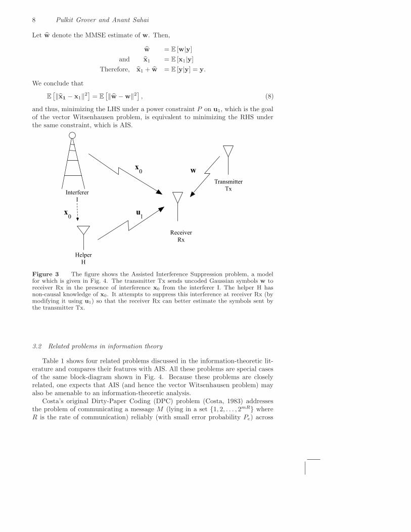
8 Pulkit Grover and Anant Sahai
Let w denote the MMSE estimate of w. Then,
w = E [w|y]
and x1 = E [x1|y]
Therefore, x1 + w = E [y|y] = y.
We conclude that
E[‖x1 − x1‖2
]= E
[‖w − w‖2
], (8)
and thus, minimizing the LHS under a power constraint P on u1, which is the goalof the vector Witsenhausen problem, is equivalent to minimizing the RHS underthe same constraint, which is AIS.
Receiver
Rx
x0
u1
x0
w
Helper
H
Interferer
I
Transmitter
Tx
Figure 3 The figure shows the Assisted Interference Suppression problem, a modelfor which is given in Fig. 4. The transmitter Tx sends uncoded Gaussian symbols w toreceiver Rx in the presence of interference x0 from the interferer I. The helper H hasnon-causal knowledge of x0. It attempts to suppress this interference at receiver Rx (bymodifying it using u1) so that the receiver Rx can better estimate the symbols sent bythe transmitter Tx.
3.2 Related problems in information theory
Table 1 shows four related problems discussed in the information-theoretic lit-erature and compares their features with AIS. All these problems are special casesof the same block-diagram shown in Fig. 4. Because these problems are closelyrelated, one expects that AIS (and hence the vector Witsenhausen problem) mayalso be amenable to an information-theoretic analysis.
Costa’s original Dirty-Paper Coding (DPC) problem (Costa, 1983) addressesthe problem of communicating a message M (lying in a set {1, 2, . . . , 2mR} whereR is the rate of communication) reliably (with small error probability Pe) across

Witsen
hausen’s
counterexa
mple
as
assisted
interferen
cesu
ppressio
n9
Table 1 A comparison of various information-theoretic problems.
Problem Reconstruct/hide Performance measures Power constraint(s) on H has M? Solved?
AIS Uncoded signal w E[‖w − w‖2
]u1 No No
DPC ((Costa, 1983)) Message M R, Pe (u1 + w) Yes Yes
Distrib. DPC (Kotagiri et al.) Message M R, Pe u1;w No No
State Amplif. ((Kim et al., 2008)) Message M , “state” x0 R,Pe, E[‖x0 − x0‖2
](u1 + w) Yes Yes
State Masking (Merhav et al.) Message M , hide x0 R,Pe, min I(x0,y2) (u1 + w) Yes Yes
10 Pulkit Grover and Anant Sahai
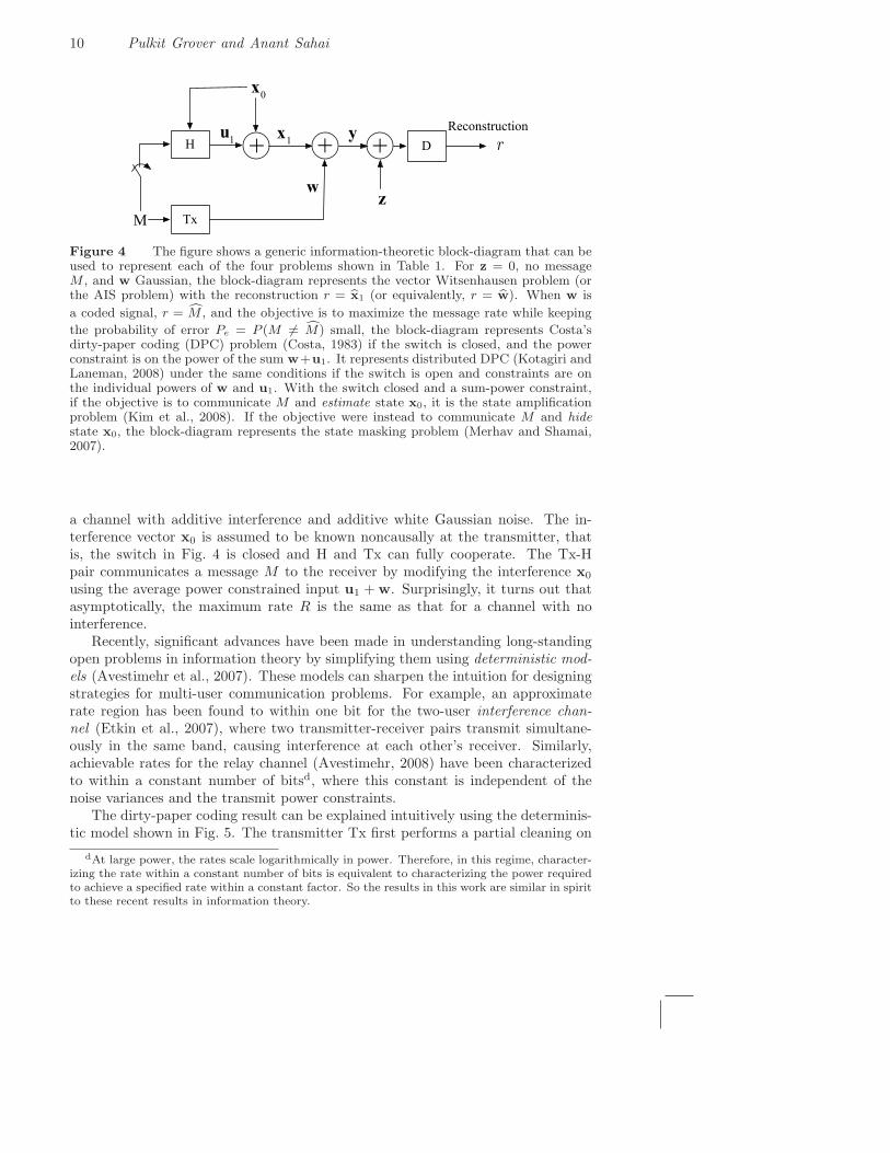
x0
++ D
z
H
w
TxM
r
Reconstructionx1
+yu
1
Figure 4 The figure shows a generic information-theoretic block-diagram that can beused to represent each of the four problems shown in Table 1. For z = 0, no messageM , and w Gaussian, the block-diagram represents the vector Witsenhausen problem (orthe AIS problem) with the reconstruction r = bx1 (or equivalently, r = bw). When w is
a coded signal, r = cM , and the objective is to maximize the message rate while keeping
the probability of error Pe = P (M 6= cM) small, the block-diagram represents Costa’sdirty-paper coding (DPC) problem (Costa, 1983) if the switch is closed, and the powerconstraint is on the power of the sum w+u1. It represents distributed DPC (Kotagiri andLaneman, 2008) under the same conditions if the switch is open and constraints are onthe individual powers of w and u1. With the switch closed and a sum-power constraint,if the objective is to communicate M and estimate state x0, it is the state amplificationproblem (Kim et al., 2008). If the objective were instead to communicate M and hidestate x0, the block-diagram represents the state masking problem (Merhav and Shamai,2007).
a channel with additive interference and additive white Gaussian noise. The in-terference vector x0 is assumed to be known noncausally at the transmitter, thatis, the switch in Fig. 4 is closed and H and Tx can fully cooperate. The Tx-Hpair communicates a message M to the receiver by modifying the interference x0
using the average power constrained input u1 + w. Surprisingly, it turns out thatasymptotically, the maximum rate R is the same as that for a channel with nointerference.
Recently, significant advances have been made in understanding long-standingopen problems in information theory by simplifying them using deterministic mod-els (Avestimehr et al., 2007). These models can sharpen the intuition for designingstrategies for multi-user communication problems. For example, an approximaterate region has been found to within one bit for the two-user interference chan-nel (Etkin et al., 2007), where two transmitter-receiver pairs transmit simultane-ously in the same band, causing interference at each other’s receiver. Similarly,achievable rates for the relay channel (Avestimehr, 2008) have been characterizedto within a constant number of bitsd, where this constant is independent of thenoise variances and the transmit power constraints.
The dirty-paper coding result can be explained intuitively using the determinis-tic model shown in Fig. 5. The transmitter Tx first performs a partial cleaning on
dAt large power, the rates scale logarithmically in power. Therefore, in this regime, character-izing the rate within a constant number of bits is equivalent to characterizing the power requiredto achieve a specified rate within a constant factor. So the results in this work are similar in spiritto these recent results in information theory.

Witsenhausen’s counterexample as assisted interference suppression 11
I6
I5
I4
I3
I2
I1
I3
B3
I2
B2
I1 B1
zero-forcing
low order bits
encoding
message bits
B3
B2
B1
I6
I5
I4
The most significant
bits of the interference
are untouched
Figure 5 The figure shows a deterministic model for dirty-paper coding in which real-valued addition is simplified to bitwise modulo-two addition by essentially dropping any“carry bits.” The bits Ii represent the interference signal. The transmitter zero-forces thelow order bits of the interference using this knowledge, and then encodes the informationbits Bi to take their place. This suggests that dirty-paper coding can be implemented ina distributed manner, since in this model the zero-forcing of the interference bits does notrequire the knowledge of the information bits, and encoding the desired information bitsdoes not require knowledge of the interference.
the channel by zero-forcing the “low order bits” of the interference vector, whichcorresponds to using a power much smaller than the potentially high interferencepower. The desired message is now encoded into these low order bits. Interestingly,this deterministic interpretation suggests that a dirty-paper coding scheme wouldwork even if the helper that cleans the channel and the transmitter that transmitsthe message are different — a situation that can be thought of as distributed dirty-paper coding. If the transmitter and the helper have equal power, the helper canclean some space for use by the transmitter, who can now communicate reliably atcapacity for the power constraint in the space cleaned up. The total power requiredis thus at most twice the power required for communicating with zero interference.This suggests that a distributed DPC implementation suffers a capacity-loss of atmost half a bit.
The distributed dirty-paper coding problem was addressed by Kotagiri andLaneman in (Kotagiri and Laneman, 2008) as a special case of the multiple accesschannel with partial state information at some encoders. The authors provide up-

12 Pulkit Grover and Anant Sahai
per bounds and lower bounds on achievable rates for the second transmitter, givenconstraints on the average powers of P and σ2
w on the two transmitters. There is,however, a subtle distinction between this problem and AIS. In distributed DPC,the second user is interested in maximizing its rate, and can code its message on thechannel. In AIS, the objective is to minimize the distortion, and the transmissionsw are uncoded Gaussian symbols.
Yet another related pair of problems are state amplification (recently solvedby Kim et al (Kim et al., 2008)) and state masking (recently solved by Merhavand Shamai (Merhav and Shamai, 2007)). For the system in Fig. 4, the objectivein (Kim et al., 2008) is to reconstruct the message and the original interference x0
at the receiver. The authors characterize the tradeoff between the rate R and themean-square error in estimating x0 under an average power constraint. The optimalstrategy splits its power — a part of it is used to amplify the state, and the rest ofit is used to communicate the message by dirty-paper coding against the amplifiedstate. The state-masking problem of (Merhav and Shamai, 2007) is the opposite— the objective is to minimize the information about x0 that can be obtainedfrom y2. The optimal strategy here turns out to attenuatee the state by using apart of the power, while using the rest of the power to communicate by dirty-papercoding against the decreased interference. The crucial distinction between theseproblems and the vector Witsenhausen problem is that for state-amplification andstate-masking the objective is to reconstruct/hide x0. In contrast, for the vectorWitsenhausen problem, the objective is to reconstruct x1. The helper H gets tomodify what is to be estimated. Interestingly, the fact that the helper does notknow the message is what seems to make the problem hard in Table 1.
4 Characterization of the optimal costs for the vector Witsenhausenproblem to within a constant factor
This section characterizes the asymptotically optimal costs for the vector Wit-senhausen problem (in the limit m → ∞) within a constant factor for all values ofproblem parameters k and σ2
0 .
Theorem 1 For the problem as stated in Section 2 with σ2w = 1, in the limit of
m → ∞, the optimal expected cost Cmin(k2) for the vector Witsenhausen problemsatisfies
1
γ1min{k2, k2σ2
0 ,σ2
0
σ20 + 1
} ≤ Cmin(k2) ≤ min{k2, k2σ20 ,
σ20
σ20 + 1
}. (9)
Alternatively, Cmin(k2) satisfies
infP≥0
k2P +((√
κ(P ) −√
P )+)2
≤
Cmin(k2) ≤ γ2 infP≥0
k2P +((√
κ(P ) −√
P )+)2
, (10)
eThe deterministic-model perspective on amplification and attenuation is that they both per-form a bit-shift operation on the interference.

Witsenhausen’s counterexample as assisted interference suppression 13
where (·)+ is shorthand for max(·, 0) and
κ(P ) =σ2
0
σ20 + 2σ0
√P + P + 1
. (11)
The factors γ1 and γ2 are no more than 11 (numerical evaluation shows that γ1 <4.45, and γ2 < 2).
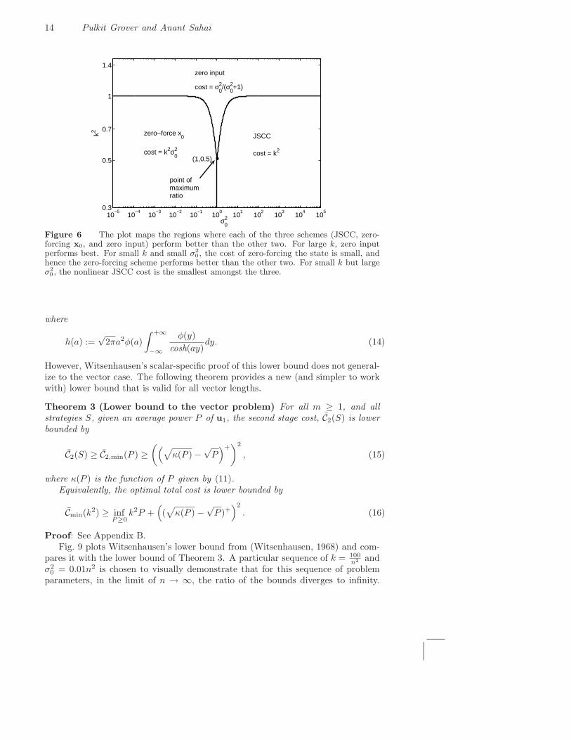
Proof: The proof proceeds in three steps. Section 4.1 states a new information-theoretic lower bound on the expected cost that is valid for all vector lengths. Thisprovides the expressions in (10). An upper bound is then derived in Section 4.2by providing three schemes, and taking the best performance among the three.This provides the expressions in (9). The first scheme (providing the k2 in (9)) isa randomized nonlinear controller that we call the Joint Source-Channel Coding(JSCC) scheme. A linear scheme that zero-forces x0 by using u1 = −x0 achieves
the second term k2σ20 . The third term of
σ2
0
σ2
0+1
is achieved by another trivial linear
scheme using u1 = 0 and performing an MMSE estimation for x1 on observing y2.Fig. 6 partitions the (k2, σ2
0) parameter space into three different regions, showingwhich of the three upper bounds is the tightest for various values of k2 and σ2
0 . It isinteresting to note that the nonlinear JSCC scheme is required only in the small-klarge-σ2
0 regime. A similar figure in (Baglietto et al., 1997, Fig. 1) for the scalarproblem shows that the same regime is interesting there as well.
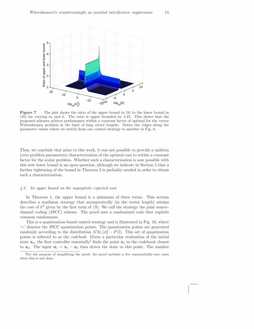
A 3-D plot of the ratio between the upper and lower bounds for varying k2 andσ2
0 is shown in Fig. 7. The figure shows that the ratio is bounded by a constantγ1, numerically evaluated to be 4.45, and attained at k2 = 0.5 and σ2
0 = 1. Thefigure also shows that for most of the (k2, σ2
0) parameter space, the ratio is in factclose to 1 so the upper and lower bounds are almost equal there. This asymptoticcharacterization can be further tightened by improving the upper bound usinga balanced combination of DPC and linear control described in Section 4.3 anddetailed in Appendix D.8. Numerical evaluation of this ratio leads us to concludethat γ2 < 2, as is illustrated in Fig. 8. The worst ratio of 2 is achieved along
σ20 =
√5−12 , the golden ratio, and k small.
Finally, Appendix E complements the plots by giving an explicit proof that theratio of the upper and lower bounds is always smaller than 11.
4.1 A lower bound on the expected cost
Witsenhausen (Witsenhausen, 1968, Section 6) derived the following lower boundon the optimal costs for the scalar problem.
Theorem 2 (Witsenhausen’s lower bound) The optimal cost for the scalarWitsenhausen counterexample is lower bounded by
Cscalar
min (k2) ≥ 1
σ0
∫ +∞
−∞φ
(ξ
σ0
)Vk(ξ)dξ, (12)
where φ(t) = 1√2π
exp(− t2
2 ) is the standard Gaussian density and
Vk(ξ) := mina
[k2(a − ξ)2 + h(a)], (13)
14 Pulkit Grover and Anant Sahai
10−5
10−4
10−3
10−2
10−1
100
101
102
103
104
105
0.3
0.5
0.7
1
1.4
σ02
k2 zero−force x0
cost = k2σ02
JSCC
cost = k2
zero input
cost = σ02/(σ
02+1)
point ofmaximumratio
(1,0.5)
Figure 6 The plot maps the regions where each of the three schemes (JSCC, zero-forcing x0, and zero input) perform better than the other two. For large k, zero inputperforms best. For small k and small σ2
0 , the cost of zero-forcing the state is small, andhence the zero-forcing scheme performs better than the other two. For small k but largeσ2
0 , the nonlinear JSCC cost is the smallest amongst the three.
where
h(a) :=√
2πa2φ(a)
∫ +∞
−∞
φ(y)
cosh(ay)dy. (14)
However, Witsenhausen’s scalar-specific proof of this lower bound does not general-ize to the vector case. The following theorem provides a new (and simpler to workwith) lower bound that is valid for all vector lengths.
Theorem 3 (Lower bound to the vector problem) For all m ≥ 1, and allstrategies S, given an average power P of u1, the second stage cost, C2(S) is lowerbounded by
C2(S) ≥ C2,min(P ) ≥((√
κ(P ) −√
P)+)2
, (15)
where κ(P ) is the function of P given by (11).Equivalently, the optimal total cost is lower bounded by
Cmin(k2) ≥ infP≥0
k2P +((√
κ(P ) −√
P )+)2
. (16)
Proof: See Appendix B.Fig. 9 plots Witsenhausen’s lower bound from (Witsenhausen, 1968) and com-
pares it with the lower bound of Theorem 3. A particular sequence of k = 100n2 and
σ20 = 0.01n2 is chosen to visually demonstrate that for this sequence of problem
parameters, in the limit of n → ∞, the ratio of the bounds diverges to infinity.
Witsenhausen’s counterexample as assisted interference suppression 15
−10−5
05
10
−20−10
010
20
1
2
3
4
5
log10
(k)log10
(σ02)
Rat
io o
f upp
er a
nd lo
wer
bou
nd
Figure 7 The plot shows the ratio of the upper bound in (9) to the lower bound in(10) for varying σ0 and k. The ratio is upper bounded by 4.45. This shows that theproposed schemes achieve performance within a constant factor of optimal for the vectorWitsenhausen problem in the limit of long vector lengths. Notice the ridges along theparameter values where we switch from one control strategy to another in Fig. 6.
Thus, we conclude that prior to this work, it was not possible to provide a uniform(over problem parameters) characterization of the optimal cost to within a constantfactor for the scalar problem. Whether such a characterization is now possible withthis new lower bound is an open question, although we indicate in Section 5 that afurther tightening of the bound in Theorem 3 is probably needed in order to obtainsuch a characterization.
4.2 An upper bound on the asymptotic expected cost
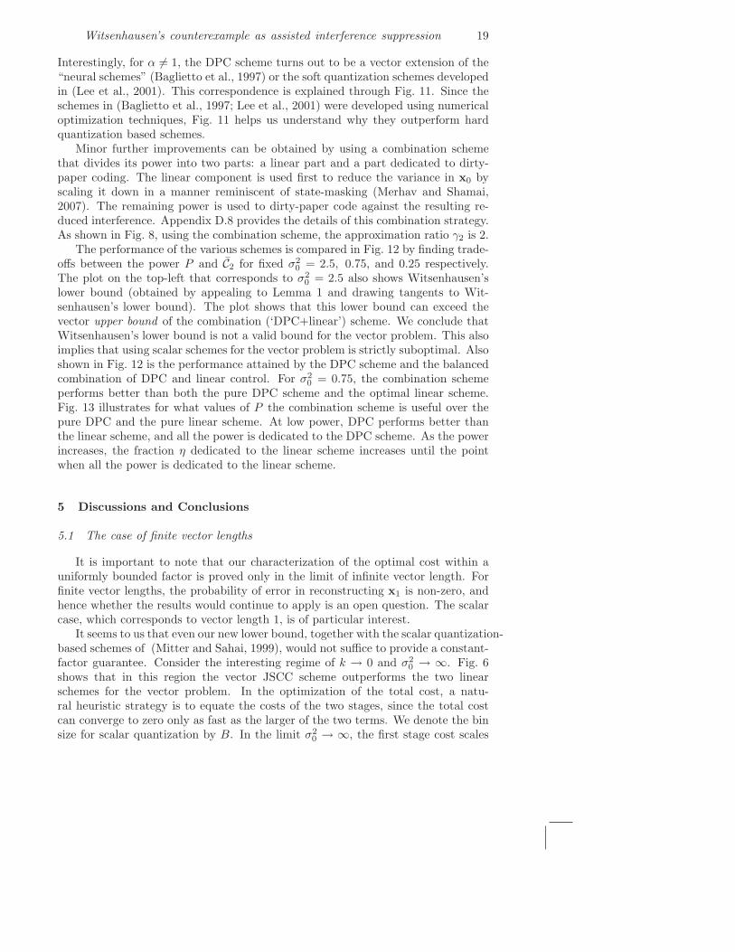
In Theorem 1, the upper bound is a minimum of three terms. This sectiondescribes a nonlinear strategy that asymptotically (in the vector length) attainsthe cost of k2 given by the first term of (9). We call the strategy the joint source-channel coding (JSCC) scheme. The proof uses a randomized code that exploitscommon randomness.
This is a quantization-based control strategy and is illustrated in Fig. 10, where‘+’ denotes the JSCC quantization points. The quantization points are generatedrandomly according to the distribution N (0, (σ2
0 − P )I). This set of quantizationpoints is referred to as the codebook. Given a particular realization of the initialstate x0, the first controller essentiallyf finds the point x1 in the codebook closestto x0. The input u1 = x1 − x0 then drives the state to this point. The number
fFor the purpose of simplifying the proof, the proof includes a few exponentially-rare caseswhen this is not done.

16 Pulkit Grover and Anant Sahai
−4
−2
0
2
−2−1
01
21
1.2
1.4
1.6
1.8
2
log10
(k)log
10(σ
02)
Rat
io o
f the
upp
er a
nd lo
wer
bou
nds
Figure 8 The plot shows the ratio of the performance of the combined DPC/linearscheme of Section 4.3 (analyzed in Appendix D.8) to the lower bound of (10) as σ0 and kvary. Relative to Fig. 7, this new scheme has a maximum ratio of 2 attained on the ridge
of σ20 =
√
5−12
and small k. Also, the ridge along k = 1 is reduced as compared to Fig. (7).
It is eliminated for small σ20 , while its asymptotic peak value of about 1.29 is attained at
k ≈ 1.68 and large σ20 .
of quantization points is chosen carefully — there are sufficiently many of them toensure that the required average power of u1 is close to P , but not so many thatthere could be confusion at the second controller. With this careful choice, we showin Appendix C that on average the state x1 can be recovered perfectly in the limitm → ∞ as long as the input power P > σ2
w = 1. Thus, asymptotically, C2 = 0,C1 = P and the total cost approaches k2.
4.3 Improved upper bound using dirty-paper coding and optimal linear scheme
In Theorem 1, for analytical simplicity, we used the JSCC scheme and two triviallinear schemes for getting an upper bound on the cost. For numerical evaluation,it is clear that optimal linear schemes can be used instead. This could certainlyimprove the cost ratio in the regime where the two linear schemes outperform theJSCC scheme in Fig. 6. However, the key small-k large-σ2
0 region is not clearbecause JSCC outperforms the two linear schemes there.
For a given value of σ20 , the cost for the optimal linear scheme is (Mitter and
Sahai, 1999, Eqn. (1))
mina
k2a2σ20 +
(1 + a)2σ20
1 + (1 + a)2σ20
. (17)
The ratio of the optimal linear cost to the k2 cost for the JSCC scheme is

Witsenhausen’s counterexample as assisted interference suppression 17
1 5 10 20 40−4
−3.5
−3
−2.5
−2
−1.5
−1
−0.5
0
n
our lower bound
Witsenhausen’s lower bound
log10(C
)
Figure 9 Plot of the two lower bounds on the optimal cost as a function of n, withkn = 100
n2 , σ0,n = 0.01n2 on a log-log scale for comparing the two lower bounds. The figureshows that the vector lower bound derived here is tighter than Witsenhausen’s scalar lowerbound in certain cases.
JSCC quantization
points
DPC quantization
points
shell oftypical source realizationsx
0
m(s - P)20 m(s +P)
20
source realization
Figure 10 A geometric representation of the joint source-channel coding scheme ofSection 4.2 and the dirty-paper coding scheme of Section 4.3 for the parameter α = 1.The grey shell contains the typical x0 realizations. The JSCC scheme quantizes to pointsinside this shell. The DPC scheme for α = 1 quantizes the state to points outside thisshell. For the same power in the input u1, the distances between the quantization pointsof the DPC scheme is larger than those for the JSCC scheme, making it robust to largerobservation noise variances.
therefore:
infa
a2σ20 +
(1 + a)2 1k2
1σ2
0
+ (1 + a)2. (18)
Now let k → 0 and σ20 → ∞. If a is close to 0, the second term is unbounded. If
a is close to −1, the first term is unbounded. For any other value of a, both termsare unbounded. Thus for any sequence of (k, σ2
0) such that k → 0 and σ20 → ∞, the

18 Pulkit Grover and Anant Sahai
Intervals in which can lie
x0
u1
x1
√
mα2σ
2
0
√
m(P + α2σ2
0)
continuum of possible values for the same quantization point
x1
values whose shadows
are attracted to the same
quantization point
x0
αx0
u1
x0
u1
x0
αx0
x1
(a) (b)
x1
Figure 11 The figure shows that the DPC scheme is a vector extension of the “softquantization” schemes found by numerical optimization techniques in (Baglietto et al.,1997; Lee et al., 2001). These scalar soft quantization schemes can be interpreted as asequence of three operations. First, as shown in the upper part of (a), the initial state x0 isscaled by a constant α. The resulting ‘shadow state’ αx0 is then quantized to the nearestquantization point. The input u1 that would force αx0 to the quantization point is thenused as the actual input at time 1. The resulting output x1 will be sloped as a functionof x0, as shown in the lower part of (a), and will take values in intervals on the y-axis.The same sequence of operations — scaling down by α, quantizing the resulting shadowstate αx0, and then using the u1 required for quantizing the shadow state as the actualinput — yields a continuum of points where x1 can take values. These values resemblesoccer-ball style caps over a sphere, in much the same way as intervals on the real line.
ratio diverges to infinity. Thus an improvement over the JSCC scheme is neededto improve the upper bound in the interesting small-k large-σ2
0 region.Such an improvement is obtained by using a nonlinear control strategy based
on the concept of dirty-paper coding (Costa, 1983). Dirty-paper coding tech-niques (Costa, 1983) can also be thought of as performing a (possibly soft) quanti-zation. The quantization points are chosen randomly in the space of realizations ofx1 according to the distribution N (0, (P + α2σ2
0)I). For α = 1 the quantization ishard and a pictorial representation is given in Fig. 10, with ‘◦’ denoting the DPCquantization points. Given the vector x0, the first controller finds the quantizationpoint x1 closest to x0 and again uses u1 = x1 − x0 to drive the state to the closestpoint. For σ2
0 > σ2w = 1, we show in Appendix D that asymptotically, C2 = 0, and
that this scheme performs better than JSCC.For α 6= 1, the transmitter does not drive the state all the way to a quantization
point. Instead, the state x1 = x0 + u1 is merely correlated with the quantizationpoint, given by v = x0 + αu1. With high probability, the second controller candecode the underlying quantization point, and using the two observations y =x0 + u1 + w and v = x0 + αu1, it can estimate x1 = x0 + u1. This scheme hasC2 6= 0, but when k is moderate, the total cost can be lower than that for DPC withα = 1. Appendix D describes this strategy and analyzes its performance in detail.
Witsenhausen’s counterexample as assisted interference suppression 19
Interestingly, for α 6= 1, the DPC scheme turns out to be a vector extension of the“neural schemes” (Baglietto et al., 1997) or the soft quantization schemes developedin (Lee et al., 2001). This correspondence is explained through Fig. 11. Since theschemes in (Baglietto et al., 1997; Lee et al., 2001) were developed using numericaloptimization techniques, Fig. 11 helps us understand why they outperform hardquantization based schemes.
Minor further improvements can be obtained by using a combination schemethat divides its power into two parts: a linear part and a part dedicated to dirty-paper coding. The linear component is used first to reduce the variance in x0 byscaling it down in a manner reminiscent of state-masking (Merhav and Shamai,2007). The remaining power is used to dirty-paper code against the resulting re-duced interference. Appendix D.8 provides the details of this combination strategy.As shown in Fig. 8, using the combination scheme, the approximation ratio γ2 is 2.
The performance of the various schemes is compared in Fig. 12 by finding trade-offs between the power P and C2 for fixed σ2
0 = 2.5, 0.75, and 0.25 respectively.The plot on the top-left that corresponds to σ2
0 = 2.5 also shows Witsenhausen’slower bound (obtained by appealing to Lemma 1 and drawing tangents to Wit-senhausen’s lower bound). The plot shows that this lower bound can exceed thevector upper bound of the combination (‘DPC+linear’) scheme. We conclude thatWitsenhausen’s lower bound is not a valid bound for the vector problem. This alsoimplies that using scalar schemes for the vector problem is strictly suboptimal. Alsoshown in Fig. 12 is the performance attained by the DPC scheme and the balancedcombination of DPC and linear control. For σ2
0 = 0.75, the combination schemeperforms better than both the pure DPC scheme and the optimal linear scheme.Fig. 13 illustrates for what values of P the combination scheme is useful over thepure DPC and the pure linear scheme. At low power, DPC performs better thanthe linear scheme, and all the power is dedicated to the DPC scheme. As the powerincreases, the fraction η dedicated to the linear scheme increases until the pointwhen all the power is dedicated to the linear scheme.
5 Discussions and Conclusions
5.1 The case of finite vector lengths
It is important to note that our characterization of the optimal cost within auniformly bounded factor is proved only in the limit of infinite vector length. Forfinite vector lengths, the probability of error in reconstructing x1 is non-zero, andhence whether the results would continue to apply is an open question. The scalarcase, which corresponds to vector length 1, is of particular interest.
It seems to us that even our new lower bound, together with the scalar quantization-based schemes of (Mitter and Sahai, 1999), would not suffice to provide a constant-factor guarantee. Consider the interesting regime of k → 0 and σ2
0 → ∞. Fig. 6shows that in this region the vector JSCC scheme outperforms the two linearschemes for the vector problem. In the optimization of the total cost, a natu-ral heuristic strategy is to equate the costs of the two stages, since the total costcan converge to zero only as fast as the larger of the two terms. We denote the binsize for scalar quantization by B. In the limit σ2
0 → ∞, the first stage cost scales

20 Pulkit Grover and Anant Sahai
like to k2 B2
12 , because the distribution of x0 conditioned on it falling in any partic-ular bin is approximately uniform. The second stage cost is the mean-square errorintroduced due to incorrect decoding. The error event corresponds to the noiserealization making x1 look like it is in a different quantization bin. The probability
of this event is approximately e−B
2
8 . Any incorrect decoding incurs a mean-square
error of at least B2. Equating the two costs, e−B
2
8 B2 ≈ k2B2
12 , suggests that the
optimal bin size B is approximately
√16 ln
(2√
3k
). The ratio of the costs for the
scalar quantization scheme and the JSCC scheme is thus approximately k2B2
6k2 = B2
6 ,which diverges since ln
(1k
)→ ∞ as k → 0.
5.2 Conclusions and further work
Using tools from information theory, the asymptotically optimal cost for thevector version of Witsenhausen’s counterexample is characterized to within a factorof 2 for all parameter values. Section 4.2 and Section 4.3 provide costs that areattained by randomized JSCC and DPC strategies. However, within the collectionof deterministic control strategies over which the randomization is being performed,there exists a deterministic strategy that attains a cost no larger than the average.So our characterization holds even when randomized strategies are not allowed.
Since such a constant-factor result is not known for the original scalar problem,we conclude that the counterexample is indeed simplified by considering the vectorextension with asymptotically long vector lengths. The results also reaffirm thenotion that implicit communication is central to Witsenhausen’s counterexample.From an information-theoretic perspective, there are three main remaining issues:closing the gap between the upper and lower bounds, understanding what happensfor finite-length vectors, and showing how to exploit known DPC codes to getreasonably good explicit nonlinear control strategies.
The tools we develop in this work might be useful in understanding generaldistributed control problems. After all, this is a positive result. So it would beinteresting to consider a more realistic version of Witsenhausen’s counterexamplewhere the first controller receives a noisy observation of the state x0, and thereare also quadratic costs associated with both x1 and u2. It might be possible tocharacterize the asymptotic costs within a constant factor for all these problems aswell.
Acknowledgments
We thank Aaron Wagner and Kristen Woyach for interesting discussions, andthe anonymous reviewers for careful reading and suggestions for improvement. Theideas contaied herein have also been enhanced by the experience of the secondauthor in co-teaching a special topics course with David Tse. We gratefully ac-knowledge the support of the National Science Foundation (CNS-403427 and CCF-729122) and Sumitomo Electric.
Witsenhausen’s counterexample as assisted interference suppression 21
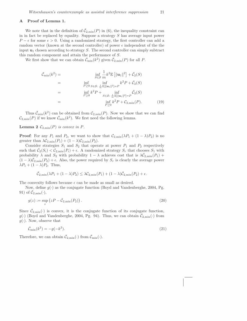
A Proof of Lemma 1.
We note that in the definition of C2,min(P ) in (6), the inequality constraint canin in fact be replaced by equality. Suppose a strategy S has average input powerP − ǫ for some ǫ > 0. Using a randomized strategy, the first controller can add arandom vector (known at the second controller) of power ǫ independent of the theinput u1 chosen according to strategy S. The second controller can simply subtractthis random component and attain the performance of S.
We first show that we can obtain Cmin(k2) given C2,min(P ) for all P .
Cmin(k2) = infS∈S
1
mk2E
[‖u1‖2
]+ C2(S)
= infP≥0
infS∈S: 1
mE[‖u1‖2]=P
k2P + C2(S)
= infP≥0
k2P + infS∈S: 1
mE[‖u1‖2]=P
C2(S)
= infP≥0
k2P + C2,min(P ). (19)
Thus Cmin(k2) can be obtained from C2,min(P ). Now we show that we can findC2,min(P ) if we know Cmin(k2). We first need the following lemma.
Lemma 2 C2,min(P ) is convex in P .
Proof: For any P1 and P2, we want to show that C2,min(λP1 + (1 − λ)P2) is nogreater than λC2,min(P1) + (1 − λ)C2,min(P2).
Consider strategies S1 and S2 that operate at power P1 and P2 respectivelysuch that C2(Si) < C2,min(Pi) + ǫ. A randomized strategy Sr that chooses S1 withprobability λ and S2 with probability 1 − λ achieves cost that is λC2,min(P1) +(1 − λ)C2,min(P2) + ǫ. Also, the power required by Sr is clearly the average powerλP1 + (1 − λ)P2. Thus,
C2,min(λP1 + (1 − λ)P2) ≤ λC2,min(P1) + (1 − λ)C2,min(P2) + ǫ.
The convexity follows because ǫ can be made as small as desired.Now, define g(·) as the conjugate function (Boyd and Vandenberghe, 2004, Pg.
91) of C2,min(·),
g(z) := supz
(zP − C2,min(P2)
). (20)
Since C2,min(·) is convex, it is the conjugate function of its conjugate function,g(·) (Boyd and Vandenberghe, 2004, Pg. 94). Thus, we can obtain C2,min(·) fromg(·). Now, observe that
Cmin(k2) = −g(−k2). (21)
Therefore, we can obtain C2,min(·) from Cmin(·).
22 Pulkit Grover and Anant Sahai
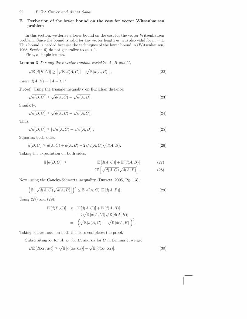
B Derivation of the lower bound on the cost for vector Witsenhausenproblem
In this section, we derive a lower bound on the cost for the vector Witsenhausenproblem. Since the bound is valid for any vector length m, it is also valid for m = 1.This bound is needed because the techniques of the lower bound in (Witsenhausen,1968, Section 6) do not generalize to m > 1.
First, a simple lemma.
Lemma 3 For any three vector random variables A, B and C,
√E [d(B,C)] ≥
∣∣∣√
E [d(A,C)] −√
E [d(A,B)]∣∣∣ , (22)
where d(A,B) = ‖A − B‖2.
Proof: Using the triangle inequality on Euclidian distance,√
d(B,C) ≥√
d(A,C) −√
d(A,B). (23)
Similarly,√
d(B,C) ≥√
d(A,B) −√
d(A,C). (24)
Thus,√
d(B,C) ≥ |√
d(A,C) −√
d(A,B)|, (25)
Squaring both sides,
d(B,C) ≥ d(A,C) + d(A,B) − 2√
d(A,C)√
d(A,B). (26)
Taking the expectation on both sides,
E [d(B,C)] ≥ E [d(A,C)] + E [d(A,B)] (27)
−2E
[√d(A,C)
√d(A,B)
]. (28)
Now, using the Cauchy-Schwartz inequality (Durrett, 2005, Pg. 13),
(E
[√d(A,C)
√d(A,B)
])2
≤ E [d(A,C)] E [d(A,B)] . (29)
Using (27) and (29),
E [d(B,C)] ≥ E [d(A,C)] + E [d(A,B)]
−2√
E [d(A,C)]√
E [d(A,B)]
=(√
E [d(A,C)] −√
E [d(A,B)])2
.
Taking square-roots on both the sides completes the proof.
Substituting x0 for A, x1 for B, and u2 for C in Lemma 3, we get√
E [d(x1,u2)] ≥√
E [d(x0,u2)] −√
E [d(x0,x1)]. (30)
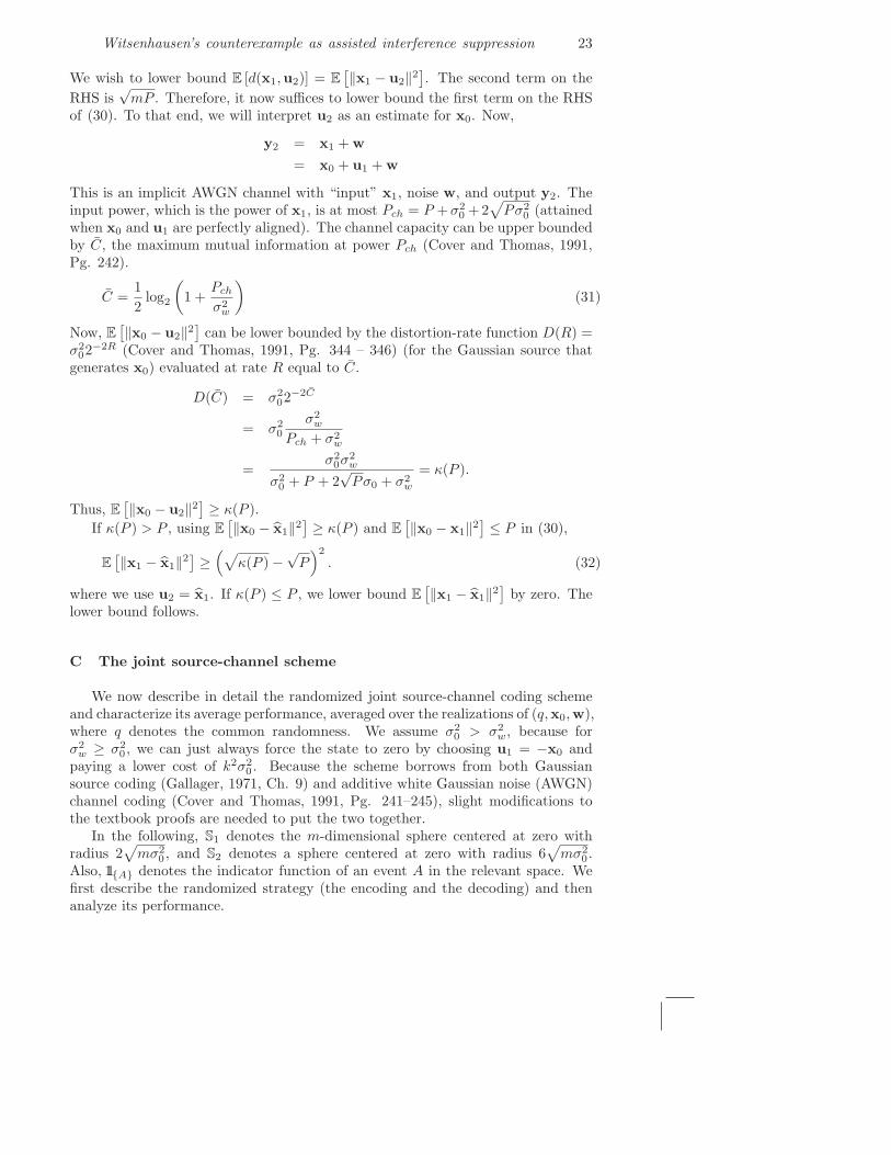
Witsenhausen’s counterexample as assisted interference suppression 23
We wish to lower bound E [d(x1,u2)] = E[‖x1 − u2‖2
]. The second term on the
RHS is√
mP . Therefore, it now suffices to lower bound the first term on the RHSof (30). To that end, we will interpret u2 as an estimate for x0. Now,
y2 = x1 + w
= x0 + u1 + w
This is an implicit AWGN channel with “input” x1, noise w, and output y2. Theinput power, which is the power of x1, is at most Pch = P +σ2
0 +2√
Pσ20 (attained
when x0 and u1 are perfectly aligned). The channel capacity can be upper boundedby C, the maximum mutual information at power Pch (Cover and Thomas, 1991,Pg. 242).
C =1
2log2
(1 +
Pch
σ2w
)(31)
Now, E[‖x0 − u2‖2
]can be lower bounded by the distortion-rate function D(R) =
σ202−2R (Cover and Thomas, 1991, Pg. 344 – 346) (for the Gaussian source that
generates x0) evaluated at rate R equal to C.
D(C) = σ202−2C
= σ20
σ2w
Pch + σ2w
=σ2
0σ2w
σ20 + P + 2
√Pσ0 + σ2
w
= κ(P ).
Thus, E[‖x0 − u2‖2
]≥ κ(P ).
If κ(P ) > P , using E[‖x0 − x1‖2
]≥ κ(P ) and E
[‖x0 − x1‖2
]≤ P in (30),
E[‖x1 − x1‖2
]≥(√
κ(P ) −√
P)2
. (32)
where we use u2 = x1. If κ(P ) ≤ P , we lower bound E[‖x1 − x1‖2
]by zero. The
lower bound follows.
C The joint source-channel scheme
We now describe in detail the randomized joint source-channel coding schemeand characterize its average performance, averaged over the realizations of (q,x0,w),where q denotes the common randomness. We assume σ2
0 > σ2w, because for
σ2w ≥ σ2
0 , we can just always force the state to zero by choosing u1 = −x0 andpaying a lower cost of k2σ2
0 . Because the scheme borrows from both Gaussiansource coding (Gallager, 1971, Ch. 9) and additive white Gaussian noise (AWGN)channel coding (Cover and Thomas, 1991, Pg. 241–245), slight modifications tothe textbook proofs are needed to put the two together.
In the following, S1 denotes the m-dimensional sphere centered at zero withradius 2
√mσ2
0 , and S2 denotes a sphere centered at zero with radius 6√
mσ20 .
Also, 11{A} denotes the indicator function of an event A in the relevant space. Wefirst describe the randomized strategy (the encoding and the decoding) and thenanalyze its performance.

24 Pulkit Grover and Anant Sahai
C.1 Codebook construction and encoding
The encoding is performed at the first controller C1. The strategy has a single
parameter δ. A list Q of 2mR +1 quantization points {xq(0),xq(1), . . . ,xq(2mR)} is
chosen by drawing the quantization points iid in Rm randomly from the distributionN (0, (σ2
0 − P )I), where the operating “rate” R and the power P satisfy the pair ofequalities
R = R(P ) +δ
2=
1
2log2(σ
20/P ) +
δ
2(33)
C(P ) =1
2log2
(1 +
σ20 − P
σ2w
)= R +
δ
2, (34)
for small δ > 0 where R(·) is the rate-distortion function for a Gaussian source ofvariance σ2
0 (Cover and Thomas, 1991, Pg. 345), and C(·) is the capacity of anAWGN channel with input power constraint σ2
0−P . That this pair of equalities hasa solution with P < σ2
0 is shown in Appendix C.4. The probability space thereforeconsists of three independent random variables, the common randomness Q, theinitial state x0 and the noise w.
The encoding now proceeds in three steps.Step 1 : In the case that Q is pathological so that the first quantization point
xq(0) /∈ S1, the encoder just uses u1 = −x0 to push the state to zero.Step 2 : If x0 /∈ S1, the encoder uses u1 = −x0 to force x0 to zero.Step 3 : If xq(0) ∈ S1 and x0 ∈ S1, the encoding is performed by finding the
quantization point x1 ∈ S2 such that
x1(x0) = arg minx∈Q∩S2
‖x0 − x‖, (35)
and using u1 = x1 − x0 to drive the state to x1.
C.2 Decoding
The decoder C2 is assumed to know the realization of Q because of the shared
common randomness.Case 1 : If xq(0) /∈ S1, the second controller decodes to zero and applies u2 = 0.Case 2 : If xq(0) ∈ S1, the second controller examines the noisy observation
y2 = x1 + w. It decodes to the quantization point x1 given by
x1(y2) = arg minx∈Q∩S2
‖y2 − x‖, (36)
and applies the control u2 = x1.
C.3 Performance analysis
We now show that the average cost of the encoding and the decoding can bemade arbitrarily close to k2σ2
w and zero respectively by choosing m large enoughand δ small enough. We first need the following lemma.
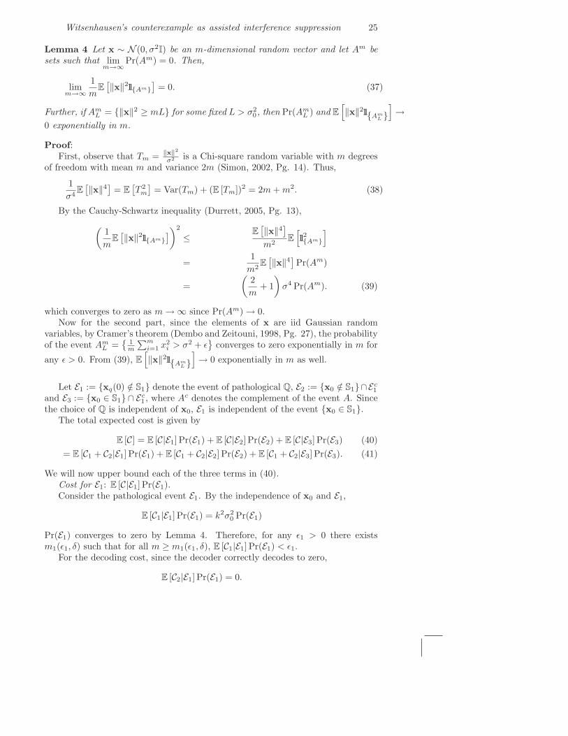
Witsenhausen’s counterexample as assisted interference suppression 25
Lemma 4 Let x ∼ N (0, σ2I) be an m-dimensional random vector and let Am besets such that lim
m→∞Pr(Am) = 0. Then,
limm→∞
1
mE[‖x‖211{Am}
]= 0. (37)
Further, if AmL = {‖x‖2 ≥ mL} for some fixed L > σ2
0, then Pr(AmL ) and E
[‖x‖211{Am
L }]→
0 exponentially in m.
Proof:First, observe that Tm = ‖x‖2
σ2 is a Chi-square random variable with m degreesof freedom with mean m and variance 2m (Simon, 2002, Pg. 14). Thus,
1
σ4E[‖x‖4
]= E
[T 2
m
]= Var(Tm) + (E [Tm])2 = 2m + m2. (38)
By the Cauchy-Schwartz inequality (Durrett, 2005, Pg. 13),
(1
mE[‖x‖211{Am}
])2
≤ E[‖x‖4
]
m2E
[112{Am}
]
=1
m2E[‖x‖4
]Pr(Am)
=
(2
m+ 1
)σ4 Pr(Am). (39)
which converges to zero as m → ∞ since Pr(Am) → 0.Now for the second part, since the elements of x are iid Gaussian random
variables, by Cramer’s theorem (Dembo and Zeitouni, 1998, Pg. 27), the probabilityof the event Am
L ={
1m
∑mi=1 x2
i > σ2 + ǫ}
converges to zero exponentially in m for
any ǫ > 0. From (39), E
[‖x‖211{Am
L }]→ 0 exponentially in m as well.
Let E1 := {xq(0) /∈ S1} denote the event of pathological Q, E2 := {x0 /∈ S1}∩Ec1
and E3 := {x0 ∈ S1} ∩ Ec1 , where Ac denotes the complement of the event A. Since
the choice of Q is independent of x0, E1 is independent of the event {x0 ∈ S1}.The total expected cost is given by
E [C] = E [C|E1] Pr(E1) + E [C|E2] Pr(E2) + E [C|E3] Pr(E3) (40)
= E [C1 + C2|E1] Pr(E1) + E [C1 + C2|E2] Pr(E2) + E [C1 + C2|E3] Pr(E3). (41)
We will now upper bound each of the three terms in (40).Cost for E1: E [C|E1] Pr(E1).Consider the pathological event E1. By the independence of x0 and E1,
E [C1|E1] Pr(E1) = k2σ20 Pr(E1)
Pr(E1) converges to zero by Lemma 4. Therefore, for any ǫ1 > 0 there existsm1(ǫ1, δ) such that for all m ≥ m1(ǫ1, δ), E [C1|E1] Pr(E1) < ǫ1.
For the decoding cost, since the decoder correctly decodes to zero,
E [C2|E1] Pr(E1) = 0.
26 Pulkit Grover and Anant Sahai
Thus the first term in (40) is smaller than ǫ1 for m ≥ m1(ǫ1, δ).Cost for E2: E [C|E2] Pr(E2).
E [C1|E2] Pr(E2) =k2
mE[‖x0‖211{E2}
],
which converges to zero as m → ∞ by Lemma 4.Since the decoder always decodes to a quantization point inside S2, which has
diameter 6√
mσ20 ,
E [C2|E2] Pr(E2) ≤ 36σ20 Pr(E2).
By Lemma 4, Pr(E2) also converges to zero.Thus the second term in (40) can be made smaller than ǫ1 for m ≥ m2(ǫ1, δ).Cost for E3: E [C|E3] Pr(E3)Gallager (Gallager, 1971, Pg. 471-472) constructs quantization codebooks for
Gaussian vectors by the same random generation as in Appendix C.1, except thatthe construction in Appendix C.1 has one extra point xq(0).
Since xq(0) ∈ S1, for any initial state realization x0 ∈ S1, ‖x0 − xq(0)‖ ≤4√
mσ20 , the diameter of S1. Also, for any x0 ∈ S1, and any quantization point
x∗q /∈ S2 , ‖x0 − x∗
q‖ ≥ 4√
mσ20 . Thus any x0 ∈ S1 is encoded to inside S2. Any
x0 /∈ S1 is encoded to 0 ∈ S2, and thus all initial state realizations are encoded towithin S2.
In (Gallager, 1971, Pg. 471-472), it is shown that for a randomly constructedsource codebook of 2mR quantization points, as long as R = R(P ) + δ for someδ > 0,
limm→∞
Pr
(1
k2C1 > P + ǫ1
)→ 0. (42)
for all ǫ1 > 0. Since adding an extra quantization point can only decrease thedistortion,
limm→∞
Pr
(1
k2C1 > P + ǫ1
∣∣∣∣E3
)→ 0. (43)
Thus, there exists m3(ǫ1, δ) such that for all m > m3(ǫ1, δ), Pr(
1k2 C1 > P + ǫ1|E3
)<
ǫ14σ2
0
. Therefore,
E [C1|E3] = E
[C1
∣∣∣∣E3,1
k2C1 > P + ǫ1
]Pr
(1
k2C1 > P + ǫ1
∣∣∣∣E3
)
+E
[C1
∣∣∣∣E3,1
k2C1 ≤ P + ǫ1
]Pr
(1
k2C1 ≤ P + ǫ1
∣∣∣∣E3
)
≤ 4σ20k2 Pr
(1
k2C1 > P + ǫ1
∣∣∣∣E3
)+ k2(P + ǫ1)
≤ k2P + 2k2ǫ1.
Thus, E [C1|E3] ≤ k2(P + 2ǫ1) for all m > m3(ǫ1, δ).

Witsenhausen’s counterexample as assisted interference suppression 27
Now we analyze the cost of decoding under the event E3. The key observationis that a randomly generated Gaussian codebook also achieves the capacity of aGaussian channel (Cover and Thomas, 1991, Pg. 244) for an average power con-straint equal to the average power of the codebook. By construction, the averagepower of the codebook, that is, 1
mE[‖x1‖2
]is σ2
0 − P . The channel capacity C fora Gaussian channel with power constraint σ2
0 − P is
C =1
2log2
(1 +
σ20 − P
σ2w
). (44)
We know that as long as log2
(2mR + 1
)< C, the average error probability E [Pe(Q)]
for a random Gaussian codebook of 2mR + 1 codewords converges to zero (Coverand Thomas, 1991, Pg. 244). There exists m4(δ) such that for all m > m4(δ),C = R + δ
2 > log2
(2mR + 1
)+ δ
4 . Now,
E [Pe(Q)] ≥ E [Pe(Q)|E3] Pr(E3) (45)
= E [Pe(Q)|E3] (1 − Pr(E1) − Pr(E2)). (46)
Since Pr(E1) and Pr(E2) converge to zero as m → ∞, 1 − Pr(E1) − Pr(E2) → 1.Also, E [Pe(Q)] → 0. Thus E [Pe(Q)|E3] → 0 as well.
In case of a decoding error, since x1 and x1 are both in S2, they are separatedby a distance no more than the diameter 12
√mσ2
0 of S2. Thus the cost introducedby decoding error is bounded as follows
E [C2|E3] ≤ 144σ20E [Pe(Q)|E3] (47)
which goes to zero as m → ∞. Thus there exists m6(ǫ1, δ) such that for all m >m6(ǫ1, δ), E [C2|E3] Pr(E3) ≤ ǫ1.
Total average cost :The total average cost is given by
E [C] = E [C1 + C2|E1] Pr(E1) + E [C1 + C2|E2] Pr(E2)
+E [C1|E3] Pr(E3) + E [C2|E3] Pr(E3)
≤ ǫ1 + ǫ1 + k2(P + 2ǫ1) + ǫ1 ≤ k2P + (3 + 2k2)ǫ1,
for m > max{m1(ǫ1, δ),m2(ǫ1, δ),m3(ǫ1, δ),m4(ǫ1, δ),m5(δ),m6(ǫ1, δ)}. Thus, byletting m → ∞, ǫ1 → 0, and the total cost converges to k2P . In the next section,we show that the required P can be made as small as σ2
w in the limit m → ∞.
C.4 Required P for error probability converging to zero
Now we calculate the required P that satisfies (33) and (34). Let ξ satisfy12 log2 (1 + ξ) = δ. Then (33) and (34) are satisfied whenever
1
2log2
(σ2
w + σ20 − P
σ2w
)=
1
2log2
(σ2
0
P
)+
1
2log2 (1 + ξ) ,
i.e.σ2
w + σ20 − P
σ2w
=σ2
0
P(1 + ξ)
i.e. P 2 − P (σ20 + σ2
w) + σ2wσ2
0(1 + ξ) = 0. (48)
28 Pulkit Grover and Anant Sahai
Now, some algebra reveals that (48) is satisfied if
P =σ2
0 + σ2w −
√(σ2
0 − σ2w)2 − 4σ2
0σ2wξ2
2
= σ20
1 −
√1 − 4σ2
0σ2
wξ2
(σ2
0−σ2
w)2
2
+ σ2w
1 +
√1 − 4σ2
0σ2
wξ2
(σ2
0−σ2
w)2
2
,
which is along the line segment joining σ2w and σ2
0 , and is hence smaller than σ20 .
For this P to exist, ξ <σ2
0−σ2
w
2σ0σw
, and δ < 12 log2
(1 +
σ2
0−σ2
w
2σ0σw
). Also, in the limit
ξ → 0 (or equivalently, δ → 0), P converges to σ2w.
D Dirty-Paper Coding (DPC) based schemes
As noted in Section 3.1, the vector Witsenhausen counterexample is similar tothe communication problem of multiaccess channels with states known to someencoders (Kotagiri and Laneman, 2008), and so the strategy we propose in thissection is also similar to that in (Kotagiri and Laneman, 2008).
D.1 A pure dirty-paper coding scheme: Encoding and decoding
Encoding :In this section, we describe the encoding and decoding of the DPC-based scheme.
The scheme has two parameters α and ǫ. The variable P is a function of α and ǫand can be evaluated from (56).
Step 1 : Generate a list Q of 2m(T−ǫ) Gaussian random vectors v ∼ N (0, P +α2σ2
0), where
T =1
2log2
((P + σ2
0 + σ2w)(P + α2σ2
0)
Pσ20(1 − α)2 + σ2
w(P + α2σ20)
). (49)
Step 2 : Given x0, the encoder C1 finds a v ∈ Q such that (v,x0) satisfy,
∣∣∣∣∣
(1
m
m∑
i=1
x20,i
)− σ2
0
∣∣∣∣∣ < ǫ
∣∣∣∣∣
(1
m
m∑
i=1
v2i
)− (P + α2σ2
0)
∣∣∣∣∣ < ǫ
∣∣∣∣∣
(1
m
m∑
i=1
x0,ivi
)− ασ2
0
∣∣∣∣∣ < ǫ. (50)
If more than one v ∈ Q satisfy (50) for the given x0, then break the tie by choosingany one such v. The control input is u1 = v−αx0. If no such v exists, we call theevent an encoding error, and the chosen u1 = −x0.
Decoding :
Witsenhausen’s counterexample as assisted interference suppression 29
The decoder C2 receives the noisy observation y2 = x0 +u1 +w. The decoding
then proceeds in two steps.Step 1 : The decoder finds a v ∈ Q such that (v,y2) satisfy
∣∣∣∣∣1
m
m∑
i=1
v2i − (P + α2σ2
0)
∣∣∣∣∣ < ǫ
∣∣∣∣∣1
m
m∑
i=1
y22,i − (σ2
0 + P + σ2w)
∣∣∣∣∣ < ǫ
∣∣∣∣∣1
m
m∑
i=1
y2,ivi − (P + ασ20)
∣∣∣∣∣ < ǫ. (51)
If no such v exists, or more than one such v’s exist, the decoder decodes to u2 = y2
and does not continue to Step 2.Step 2 : If α = 1, the decoder declares v as the decoded codeword and sets
u2 = v.If α 6= 1, the decoder estimates the component x1,i using the column vector ζi
of length 2, where
ζ1,i = vi,
ζ2,i = y2,i = u1,i + x0,i + wi. (52)
The estimate is given by
x1,i = Qζi = q1ζ1,i + q2ζ2,i. (53)
where Q = [q1, q2] = Kx1ζK−1ζ , where
Kx1ζ = [P + ασ20 , P + σ2
0 ],
and
Kζ =
[P + α2σ2
0 P + ασ20
P + ασ20 P + σ2
0 + σ2w
].
The second control u1 = x1.Simple manipulations reveal that the determinant of Kζ is α2(σ2
0 + σ2w) + (α −
1)2Pσ20 + Pσ2
w, which is strictly positive for all values of α. Thus Kζ is alwaysinvertible.
D.2 Probability of encoding/decoding error
Let E1 denote the event of encoding error, E2 the event of successful encodingand decoding error, and E3 the event of successful encoding and correct decoding.
Let v = u1 + αx0 represent an auxiliary random variable, where u1 and x0 areindependent random variables with u1 ∼ N (0, P ) and x0 ∼ N (0, σ2
0). The variableT in the number of codewords 2n(T−ǫ) is then given by
T = I(v; y2), (54)

30 Pulkit Grover and Anant Sahai
where y2 = x0 + u1 + w. With this interpretation, the encoding is based on findingv that is ǫ-jointly typicalg with x0. The joint-typicality conditions (Gamal andCover, 1980),
∣∣∣∣−1
mlog2 (fv(v)) − h(v)
∣∣∣∣ < η1(ǫ)
∣∣∣∣−1
mlog2 (fx0
(x0)) − h(x0)
∣∣∣∣ < η1(ǫ)
∣∣∣∣−1
mlog2 (fv,x0
(v,x)) − h(v, x0)
∣∣∣∣ < η3(ǫ),
for appropriate ηj(ǫ), j = 1, 2, 3, are equivalent to the conditions in (50). Here fv(·)represents the pdf of v, and similarly for x0 and (v, x0), and h(·) is the differentialentropy function.
Now, by the weak-law of large numbers, for x0 and v generated indepen-dently, the probability that the two are ǫ-jointly typical is bounded below by(1− ǫ)2−m(I(v;x0)+3ǫ) for m large (Cover and Thomas, 1991, Pg. 195). The numberof v-codewords is 2m(I(v;y2)−ǫ). If
I(v; y2) = I(v;x0) + 5ǫ, (55)
which is equivalent to
C(α, P ) =1
2log2
(P (P + σ2
0 + σ2w)
Pσ20(1 − α)2 + σ2
w(P + α2σ20)
)= 5ǫ, (56)
then the average number of v-codewords jointly typical with a typical x0 increasesexponentially in m, and the probability of encoding error Pr(E1) decreases to zeroexponentially in m (Cover and Thomas, 1991, Pg. 353–356). That (56) has asolution is shown in Appendix D.5.
The decoding fails in two cases. If the encoding fails, so might the decoding,but since the error probability of encoding error decreases to zero exponentially, sodoes the probability of this kind of decoding error.
If the encoding succeeds, the transmitted v can be decoded correctly as longas the rate is smaller than the mutual information across the (v, y2) “channel.”Since the number of v codewords is 2m(I(v;y2)−ǫ), the rate for the v-codebook isRv = I(v; y2) − ǫ which is clearly smaller than I(v; y2). Thus the probabilityof decoding error conditioned on the success of the encoding converges to zeroexponentially in m. Since Pr(Ec
1) → 1, the probability Pr(E2) → 0 as well.
D.3 Encoding cost analysis
The average total cost is given by
E [C] = E [C1 + C2]
= E [C1|E1] Pr(E1) + E [C1|E2 ∪ E3] Pr(E2 ∪ E3)
+ E [C2|E1] Pr(E1) + E [C2|E2] Pr(E2) + E [C2|E3] Pr(E3).
gWe refer the reader to (Gamal and Cover, 1980, Pg. 226) for a tutorial on typicality andjoint-typicality.

Witsenhausen’s counterexample as assisted interference suppression 31
We will first calculate the encoding costs, followed by the decoding costs.For the event E1,
E [C1|E1] Pr(E1) =k2
mE[‖x0‖211{E1}
]→ 0
by Lemma 4, since Pr(E1) → 0. Thus, for any given ǫ1 > 0, there exists m0(ǫ, ǫ1)such that for all m > m0(ǫ, ǫ1), E [C1|E1] Pr(E1) < ǫ1.
For E2 ∪ E3, the event of successful encoding, since u = v − αx0 for (v,x)satisfying (50),
1
mE[‖u1‖2|E2 ∪ E3
]=
1
mE[‖v‖2 + α2‖x0‖2 − 2αvT x0|E2 ∪ E3
]
≤ P + α2σ20 + ǫ + α2(σ2
0 + ǫ)
−2α(ασ20) + 2|α|ǫ = P + (1 + |α|)2ǫ.
Thus E [C1|E2 ∪ E3] Pr(E2 ∪E3) ≤ k2(P +(1+ |α|)2ǫ). Thus the total encoding costsare also bounded by k2(P + (1 + |α|)2ǫ) + ǫ1.
D.4 Decoding cost analysis for α = 1
We first concentrate on the easier case α = 1.For the event E1, since u = −x0, and x1 = 0. There are two cases, the decoder
decodes to some erroneous v, or the decoder fails to decode and uses u2 = y2.Therefore,
E[C211{E1}
]≤ m−1E
[max{‖v − 0‖2, ‖y2 − 0‖2}11{E1}
]
≤ m−1E[(‖v‖2 + ‖y2‖2)11{E1}
]
(a)
≤ E[(P + α2σ2
0 + ǫ)11{E1}]+ m−1E
[‖w‖211{E1}
]
= (P + α2σ20 + ǫ) Pr(E1) + m−1E
[‖w‖211{E1}
]
where (a) follows from (51) because the decoded v is inside a sphere of radius√m(P + σ2
0 + ǫ), and under E1, y2 = w. Since Pr(E1) → 0 as m → ∞, the firstterm goes to zero. Similarly, the second term goes to zero by Lemma 4. Thus thereexists m1(ǫ, ǫ1) such that for all m > m1(ǫ, ǫ1), E [C2|E1] Pr(E1) < ǫ1.
For the event E2, again, there are the two cases of erroneous decoding anddecoding failure. Thus
E[C211{E2}
]≤ m−1E
[max{‖v − v‖2, ‖y2 − v‖2}11{E2}
]
≤ m−1E[‖v − v‖211{E2}
]+ m−1E
[‖w‖211{E2}
]
≤ 4(P + α2σ20 + ǫ) Pr(E2) + m−1E
[‖w‖211{E2}
].
The first term goes to zero because Pr(E2) → 0. The second term goes to zeroby Lemma 4. Thus for given ǫ1 > 0, there exists m2(ǫ, ǫ1) such that for all m >m2(ǫ, ǫ1), E [C2|E2] Pr(E2) < ǫ1.
For the event E3, the encoding is successful and the decoding is correct, thereforev = v, and thus E [C2|E3] = 0.

32 Pulkit Grover and Anant Sahai
D.5 Total costs for α = 1
For α = 1, for m > max{m0(ǫ, ǫ1),m1(ǫ, ǫ1),m2(ǫ, ǫ1)}, E [C2] ≤ 3ǫ1, andE [C1] ≤ k2(P + 4ǫ) + ǫ1, and the total (encoding and decoding) cost for α = 1is therefore smaller than
k2(P + 4ǫ) + 4ǫ1. (57)
Making m large enough, ǫ1 can be made as small as desired. Using the fact thatthis holds for all ǫ, in the following, we show that letting ǫ → 0, the achievable
asymptotic cost is k2σ20
r
1+4σ2
w
σ20
−1
2 .
From (56), for α = 1, P needs to satisfy C(1, P ) = 5ǫ, where
C(1, P ) =1
2log2
(P (P + σ2
0 + σ2w)
(P + σ20)σ
2w
). (58)
Let ξ be such that ǫ = 110 log2 (1 + ξ). Then,
1
2log2
(P (P + σ2
0 + σ2w)
(P + σ20)σ2
w
)=
1
2log2 (1 + ξ)
i.e. P 2 + (σ20 − ξσ2
w)P − (1 + ξ)σ20σ2
w = 0
Taking the positive root of the quadratic equation,
P = (σ20 − ξσ2
w)
√1 +
4(1+ξ)2σ2w
σ2
0
(σ2
0−ξσ2
w)2
− 1
2. (59)
Now letting ǫ go to zero (and thus ξ → 0) by increasing m to infinity, the required
P approaches σ20
r
1+4σ2
w
σ20
−1
2 . The asymptotic expected cost for the scheme is, there-
fore, k2σ20
r
1+4σ2
w
σ20
−1
2 . This expression turns out to be an increasing function in σ20
which is bounded above by k2σ2w, the cost for the JSCC scheme. Thus even in
the special case of α = 1, the DPC scheme asymptotically outperforms the JSCCscheme.
Witsenhausen’s counterexample as assisted interference suppression 33
D.6 Decoding cost analysis for α 6= 1
For the event E1, similar to the analysis of α = 1, there are the two cases ofdecoding failure and decoding error,
E[C211{E1}
]≤ 1
mE[max{‖q1v + q2w‖2, ‖y − 0‖2}11{E1}
]
≤ 1
mE[‖q1v + q2w‖211{E1}
]+
1
mE[‖w‖211{E1}
](60)
=q21
mE[‖v‖211{E1}
]+
q22
mE[‖w‖211{E1}
]
+2q1q2
mE[vT w11{E1}
]+
1
mE[‖w‖211{E1}
](61)
=q21(P + σ2
0 + ǫ)
mE[11{E1}
]+
q22
mE[‖w‖211{E1}
](62)
+2q1q2
mE[vT w11{E1}
]+
1
mE[‖w‖211{E1}
]. (63)
As m → ∞, the first term converges to zero since Pr(E1) → 0. The second termand the fourth terms converge to zero by an application of Lemma 4 with x = w.Looking at the third term in (63),
m−1E[vT w11{E1}
]= m−1E
[(
m∑
i=1
viwi)11{E1}
]
(a)
≤ m−1E[‖v‖‖w‖11{E1}
]
≤ m−1
(√P + σ2
0 + ǫ
)E
[√‖w‖211{E1}
]
(b)
≤ m−1√
P + σ20 + ǫ
√E[‖w‖211{E1}
]
where (a) follows from the Cauchy-Schwartz inequality, and (b) follows from Jensen’sinequality. By Lemma 4, the third term now converges to zero as well. There-fore, for all ǫ1 > 0, there exists m3(α, ǫ, ǫ1) such that for all m > m3(α, ǫ, ǫ1),E [C2|E1] Pr(E1) < ǫ1.
Similarly, for the event E2,
E[C211{E2}
]≤ m−1E
[max{‖q1v + q2v‖2, ‖y − v‖2}11{E2}
]
≤ m−1E[‖q1v + q2v‖211{E2}
]+ m−1E
[‖w‖211{E2}
]
≤ m−1E[(q2
1‖v‖2 + q22‖v‖2 + 2q1q2‖v‖ ‖v‖)11{E2}
]+ m−1E
[‖w‖211{E2}
]
≤ (P + α2σ20 + ǫ)(q1 + q2)
2 Pr(E2) + m−1E[‖w‖211{E2}
].
The first term converges to zero as Pr(E2) converges to zero. The second convergesto zero by an application of Lemma 4. Thus there exists m4(α, ǫ, ǫ1) such that forall m > m4(α, ǫ, ǫ1), E [C2|E2] Pr(E2) < ǫ1.
For the event E3, we need the following lemma.

34 Pulkit Grover and Anant Sahai
Lemma 5 For vectors v and x, if (v,x) are ǫ-jointly typical as defined by (50),then for u = v − αx,
|m∑
i=1
u1,ix0,i
m| < (|α| + 1)ǫ, (64)
and
|m∑
i=1
u21,i
m| < P + (1 + |α|)2ǫ. (65)
Proof: Since (v,x) are ǫ-jointly typical, using (50),
∣∣∣∣∣
m∑
i=1
vix0,i
m− ασ2
0
∣∣∣∣∣ < ǫ
i.e.
∣∣∣∣∣
m∑
i=1
(u1,i + αx0,i)x0,i
m− ασ2
0
∣∣∣∣∣ < ǫ
i.e.
∣∣∣∣∣
m∑
i=1
u1,ix0,i
m+ α
m∑
i=1
x20,i
m− ασ2
0
∣∣∣∣∣ < ǫ
i.e.
∣∣∣∣∣
m∑
i=1
u1,ix0,i
m+ α
(m∑
i=1
x20,i
m− σ2
0
)∣∣∣∣∣ < ǫ.
By the ǫ−typicality of x in (50), the term in brackets is bounded by ǫ in abso-lute value. Thus, (64) follows and asymptotically, u1 and x0 appear statisticallyuncorrelated.
Similarly, for u = v − αx0,
1
m‖u‖2 =
1
m
(‖v‖2 + α2‖x0‖2 − 2α
m∑
i=1
vix0,i
)
≤ (P + α2σ20 + ǫ) + α2(σ2
0 + ǫ) − 2α(ασ2) + 2|α|ǫ= P + (1 + |α|)2ǫ.
Now, for E3, the normalized mean-square error is given by
m−1E[‖x1 − x1‖2|E3
]
= m−1E[‖Qζ − x1‖2|E3
]
= m−1E[‖q1v + q2y2 − x1‖2|E3
]
= m−1E[‖q1(u1 + αx0) + q2(u1 + x0 + w) − x1‖2|E3
]
= m−1E[‖(q1 + q2 − 1)u1 + (αq1 + q2 − 1)x0 + q2w‖2|E3
]
= m−1
((q1 + q2 − 1)2E
[‖u1‖2|E3
]+ (αq1 + q2 − 1)2E
[‖x0‖2|E3
]+ q2
2E[‖w‖2|E3
]
+ 2(q1 + q2 − 1)(αq1 + q2 − 1)E[uT
1 x0|E3
]+ 2(q1 + q2 − 1)q2E
[uT
1 w|E3
]
+ 2(αq1 + q2 − 1)q2E[xT
0 w|E3
]), (66)

Witsenhausen’s counterexample as assisted interference suppression 35
where (·)T denotes the transpose of the vector. Now,
m−1E[uT
1 w]
= 0 = m−1E[uT
1 w|E3
]Pr(E3) + m−1E
[uT
1 w|Ec3
]Pr(Ec
3)
i.e. m−1∣∣E[uT
1 w|E3
]∣∣Pr(E3) = m−1∣∣E[uT
1 w|Ec3
]∣∣Pr(Ec3)
= m−1E
[uT
1 w11{Ec
3}]
(a)
≤√
1
m2E[(uT
1 w)2]E
[11{Ec
3}].
where (a) follows from the Cauchy-Schwartz inequality. Now,
1
m2E
[(uT
1 w)2]
=1
m2E
[(
m∑
i=1
u1,iwi)2
]
(b)=
1
m2E
[m∑
i=1
u21,iw
2i
]
(c)=
1
m2
m∑
i=1
E[u2
1,i
]σ2
w
=1
m2E
[m∑
i=1
u21,i
]σ2
w =1
m2E[‖u‖2
]σ2
w
where (b) and (c) follow from the fact that u1,i and wj are uncorrelated, and wi iszero mean. Now,
E[‖u‖2
]= E
[‖u‖211{Ec
1}]
+ E[‖u‖211{E1}
]
≤ m(P + (1 + |α|)2ǫ) Pr(Ec1) + E
[‖x0‖211{E1}
]
≤ m(P + (1 + |α|)2ǫ) + E[‖x0‖2
]
≤ m(P + (1 + |α|)2ǫ + σ20).
Thus,
1
m2E[(uT
1 w)2]E
[11{Ec
3}]≤ 1
m(P + (1 + |α|)2ǫ + σ2
0) Pr(Ec3). (67)
Since Pr(Ec3) → 0 as m → ∞, m−1E
[uT
1 w|E3
]→ 0 as m → ∞. Similarly,
m−1E[xT
0 w|E3
]also converges to zero. Using these results and Lemma 5 for
m−1E[uT
1 x0|E3
], there exists m5(α, ǫ, ǫ1) such that for all m > m5(α, ǫ, ǫ1), the
last three terms in (66) are smaller than ǫ1.Thus using the ǫ−joint typicality of v and x0 (50),
1
mE[‖x1 − x1‖2|E3
]
≤ (q1 + q2 − 1)2(P + (1 + |α|)2ǫ) + (αq1 + q2 − 1)2(σ20 + ǫ) + q2
2σ2w + ǫ1
≤ (q1 + q2 − 1)2P + (αq1 + q2 − 1)2σ20 + q2
2σ2w + ǫM(q1, q2) + ǫ1 (68)
where the constant ǫM(q1, q2) = ǫ((q1 + q2 − 1)2(1 + |α|)2 + (αq1 + q2 − 1)2
)→ 0
as ǫ → 0.
36 Pulkit Grover and Anant Sahai
Now suppose the random variables x′0 ∼ N (0, σ2
0I) and u′1 ∼ N (0, P I) are
independent of w′ ∼ N (0, σ2wI) and jointly Gaussian with covariance between u′
1
and x′0 zero. Also define v′ = u′ +αx′
0 and y′ = x′0 +u′
1 +w′. A simple calculationshows that E
[‖q1v
′ + q2y′2 − x′
1‖2]
yields the same expression as in (68) withoutthe ǫM and the ǫ1 terms. Observe that the estimation procedure in (53) is theMMSE estimation for x′
1 = x′0 + u′
1 on observing y′2, where the average error is
given by MMSEG(α, P ) is given by (Kay, 1998, Pg. 382)
MMSEG(α, P ) = Kx1− Kx1ζK
−1ζ Kx1ζ , (69)
where,
Kx1= E
[x2
1
]= P + σ2
0 . (70)
D.7 Total costs for α 6= 1
For fixed α and ǫ, if m > {m3(α, ǫ, ǫ1),m4(α, ǫ, ǫ1),m5(α, ǫ, ǫ1)}, the total costis smaller than
k2(P + (1 + |α|)2) + MMSE(α, P ) + M(q1, q2)ǫ + ǫ1, (71)
where P satisfies
C(α, P ) = I(v; y2) − I(v;x0) =1
2log2
(P (P + σ2
0 + σ2w)
Pσ20(1 − α)2 + σ2
w(P + α2σ20)
)= 5ǫ.
By arguments analogous to those in Appendix D.5, the existence of a solution canbe proved. Here we concentrate on the case of interest of ǫ → 0 by letting m → ∞.The condition (56) is then equivalent to
P (P + σ20 + σ2
w) = Pσ20(1 − α)2 + σ2
w(P + α2σ20).
Taking the positive root,
P =
√σ2
0α(2 − α)
2
(√
1 +4σ2
w
σ20(2 − α)2
− 1
)(72)
By letting m → ∞, we can have ǫ1 → 0 and also ǫ → 0. Optimizing the totalcost over α, the asymptotic total cost achieved is
minα,P
k2P + MMSE(α, P ), (73)
for P satisfying (72).
D.8 A combination of the linear scheme and the DPC scheme
While the DPC scheme outperforms the linear scheme for high values of σ20 ,
Fig. 12 shows that this is not true for low values of σ20 . It is natural to think that a
combination of the linear scheme and the DPC scheme might perform better thaneither one alone.
Witsenhausen’s counterexample as assisted interference suppression 37
Our approach is to divide the power available and dedicate a part of it to eachscheme. A linear term u1,1 = −βx0 constitutes a part of u1. This term can bethought of as changing the variance of the initial state x0. To this, we add a vectoru1,2 that is dirty-paper coded against (1 − β)x0. By Lemma 5, u1,2 is statisticallyuncorrelated with (1 − β)x0, and hence uncorrelated with u1,1 as well. Thus, thetotal power is β2σ2
0 + 1m
E[‖u1,2‖2
]+ ǫ, and this is constrained to be smaller than
P . The state x1 is, therefore,
x1 = (1 − β)x0 + u1,2, (74)
where u1,2 is the input that dirty-paper codes against (1 − β)x0. Again, ǫ → 0as m → ∞. It turns out that the optimizing β ≥ 0, consistent with the intuitionthat the power in the initial state x0 should be decreased before using dirty-papercoding against the state.
E The vector schemes perform within a constant factor of the optimal
The performance of the scheme that zero-forces x0 and the JSCC scheme isidentical for σ2
0 = 1, as is evident from Fig. 6. Therefore, we consider two differentcases: σ2
0 ≤ 1 and σ20 ≥ 1. In either case, we show that the ratio is bounded by
11. The result can be tightened by a more detailed analysis by dividing the (k, σ20)
space into finer partitions. However, we do not present the detailed analysis herefor ease of exposition.
Region 1 : σ20 ≤ 1.
We consider the upper bound as the minimum of k2σ20 and
σ2
0
σ2
0+1
. Consider the
lower bound
C ≥ minP≥0
k2P +
((√κ(P ) −
√P)+)2
. (75)
Now if the optimizing power P is greater than σ20/11, then the first term of the
lower bound is greater than k2σ20/11. Thus the ratio of the upper bound k2σ2
0 andthe lower bound is smaller than 11.
If the optimizing P ≤ σ2
0
11 ,
κ(P ) =σ2
0
(σ0 +√
P )2 + 1
≥ σ20(
σ0 + σ0√11
)2
+ 1
(σ2
0≤1)
≥ σ20(
1 + 1√11
)2
+ 1≥ 0.37σ2
0
which is greater than σ20/11 > P . Thus,
((√
κ(P ) −√
P )+)2
≥(√
0.37σ20 −
√σ2
0
11
)2
> 0.094σ20 >
σ20
11.

38 Pulkit Grover and Anant Sahai
The lower bound is no smaller than((√
κ(P ) −√
P )+)2
. Thus, even for P ≤ σ2
0
11
the ratio of the upper boundσ2
0
σ2
0+1
and the lower bound is smaller than 11.
Region 2 : σ20 ≥ 1.
The upper bound relevant here is the minimum of k2 andσ2
0
σ2
0+1
. Again, looking
at (75), if P > 111 , the ratio of the upper bound k2 to the lower bound is no more
than 11.Now, if P ≤ 1
11 ,
κ(P ) ≥ σ20
(σ0 + 1/√
11)2 + 1.
Therefore,
((√
κ(P ) −√
P )+)2
=
(√
σ20
(σ0 + 1√11
)2 + 1− 1√
11
)+
2
.
For σ20 ≥ 1, the first term on the RHS attains its minima at σ2
0 = 1. Evaluated atthis point, the term is larger than 1√
11. Therefore, a bound on the ratio for P < 1
11
is
σ20/(σ2
0 + 1)(√
σ2
0
(σ0+1
√
11)2+1
− 1√11
)2 ≤ 1(√
σ2
0
(σ0+1
√
11)2+1
− 1√11
)2
≤ 1(√
1(1+ 1
√
11)2+1
− 1√11
)2
≈ 10.56 < 11.
Thus, for σ20 ≥ 1, the ratio is bounded by 11 as well. Therefore, γ1 and γ2 are both
smaller than 11.
References
Witsenhausen H S, 1968 A counterexample in stochastic optimum control. SIAMJournal on Control 6 131–147.
Bansal R and Basar T, 1987 Stochastic teams with nonclassical information re-visited: When is an affine control optimal? IEEE Transactions on AutomaticControl 32 554–559.
Baglietto M, Parisini T and Zoppoli R, 1997 Nonlinear approximations for thesolution of team optimal control problems. Proceedings of the IEEE Conferenceon Decision and Control CDC 4592–4594.
Lee J T, Lau E and Ho Y C L, 2001 The Witsenhausen counterexample: A hi-erarchical search approach for nonconvex optimization problems. IEEE Trans.Automat. Contr. 46.

Witsenhausen’s counterexample as assisted interference suppression 39
Ho Y C and Chang T, 1980 Another look at the nonclassical information structureproblem. IEEE Transactions on Automatic Control .
Papadimitriou C H and Tsitsiklis J N, 1986 Intractable problems in control theory.SIAM Journal on Control and Optimization 24 639–654.
Rotkowitz M, 2006 Linear controllers are uniformly optimal for the witsenhausencounterexample. Proceedings of the 45th IEEE Conference on Decision and Con-trol CDC 553–558.
Ho Y C, Kastner M P and Wong E, 1978 Teams, signaling, and information theory.IEEE Trans. Automat. Contr. 23 305–312.
Mitter S K and Sahai A, 1999 Information and control: Witsenhausen revisited, inLearning, Control and Hybrid Systems: Lecture Notes in Control and InformationSciences 241 (edited by Y Yamamoto and S Hara), 281–293 (Springer, New York,NY).
Martins N C, 2006 Witsenhausen’s counter example holds in the presence of sideinformation. Proceedings of the 45th IEEE Conference on Decision and ControlCDC 1111–1116.
Tatikonda S, 2000 Control Under Communication Constraints, Ph.D. thesis, Mas-sachusetts Institute of Technology, Cambridge, MA.
Costa M, 1983 Writing on dirty paper. IEEE Trans. Inform. Theory 29 439–441.
Merhav N and Shamai S, 2007 Information rates subject to state masking. IEEETrans. Inform. Theory 53 2254–2261.
Kim Y H, Sutivong A and Cover T M, 2008 State amplification. IEEE Trans.Inform. Theory 54 1850–1859.
Avestimehr A, Diggavi S and Tse D, 2007 A deterministic approach to wirelessrelay networks, in Proc. of the Allerton Conference on Communications, Controland Computing.
Etkin R, Tse D and Wang H, 2007 Gaussian interference channel capacity to withinone bit. Submitted to IEEE Transactions on Information Theory .
Avestimehr A, 2008 Wireless Network Information Flow: A Deterministic Ap-proach, Ph.D. thesis, UC Berkeley, Berkeley, CA.
Witsenhausen H S, 1971 Separation of estimation and control for discrete timesystems. Proceedings of the IEEE 59 1557–1566.
Devroye N, Mitran P and Tarokh V, 2006 Achievable rates in cognitive radio chan-nels. IEEE Trans. Inform. Theory 52.
Jovicic A and Viswanath P, 2006 Cognitive radio: An information-theoretic per-spective, in Proceedings of the 2006 International Symposium on InformationTheory, Seattle, WA.
40 Pulkit Grover and Anant Sahai
Kotagiri S and Laneman J, 2008 Multiaccess channels with state known to someencoders and independent messages. EURASIP Journal on Wireless Communi-cations and Networking .
Boyd S and Vandenberghe L, 2004 Convex Optimization (Cambridge UniversityPress).
Durrett R, 2005 Probability: Theory and Examples, 1st edn. (Brooks/Cole, Bel-mont, CA).
Cover T M and Thomas J A, 1991 Elements of Information Theory, 1st edn. (Wiley,New York).
Gallager R G, 1971 Information Theory and Reliable Communication (John Wiley,New York, NY).
Simon M, 2002 Probability Distributions Involving Gaussian Random Variables(Springer).
Dembo A and Zeitouni O, 1998 Large Deviations Techniques and Applications(Springer).
Gamal A E and Cover T, 1980 Multiple user information theory. IEEE Trans.Inform. Theory 68 1466–1483.
Kay S M, 1998 Fundamentals of statistical signal processing: Detection theory, vol. 2(Printice Hall PTR).
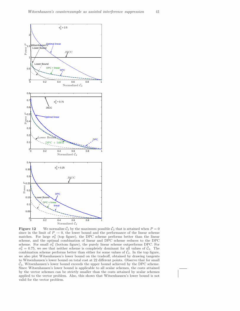
Witsenhausen’s counterexample as assisted interference suppression 41
0 0.2 0.4 0.6 0.8 10
0.5
1
1.5
2
DPC + linearDPC
Lower Bound
Optimal linear
σ02 = 2.5
Witsenhausen’sLower Bound
Pow
er
P
Normalized C2
JSCC
0 0.2 0.4 0.6 0.8 10
0.1
0.2
0.3
0.4
0.5
0.6
0.7
0.8
σ02 = 0.75
JSCC
Optimal linear
DPC
Pow
er
P
Lower Bound
DPC + linear
Normalized C2
0 0.2 0.4 0.6 0.8 10
0.05
0.1
0.15
0.2
0.25
0.3
0.35
0.4
DPC
linear
Lower Bound
σ02 = 0.25
DPC + linear
Normalized C2
Pow
er
P
JSCC
Figure 12 We normalize C2 by the maximum possible C2 that is attained when P = 0since in the limit of P → 0, the lower bound and the performance of the linear schemematches. For large σ2
0 (top figure), the DPC scheme performs better than the linearscheme, and the optimal combination of linear and DPC scheme reduces to the DPCscheme. For small σ2
0 (bottom figure), the purely linear scheme outperforms DPC. Forσ2
0 = 0.75, we see that neither scheme is completely dominant for all values of C2. Thecombination scheme performs better than either for some values of C2. In the top figure,we also plot Witsenhausen’s lower bound on the tradeoff, obtained by drawing tangentsto Witsenhausen’s lower bound on total cost at 22 different points. Observe that for smallC2, Witsenhausen’s lower bound exceeds the upper bound achieved by the DPC scheme.Since Witsenhausen’s lower bound is applicable to all scalar schemes, the costs attainedby the vector schemes can be strictly smaller than the costs attained by scalar schemesapplied to the vector problem. Also, this shows that Witsenhausen’s lower bound is notvalid for the vector problem.

42 Pulkit Grover and Anant Sahai
0 0.1 0.2 0.3 0.4 0.50
0.1
0.2
0.3
0.4
0.5
0.6
0.7
0.8
0.9
1
Power
η =
Fra
ctio
n of
pow
er d
edic
ated
to li
near
par
t
σ02 = 0.75
Figure 13 η denotes the fraction of power that is dedicated to the linear scheme. Inthe optimal combination of DPC/linear control, η is close to 1 for low P , implying thatall the power is dedicated to the linear part. As η increases, the power is shared betweenDPC and linear control, until at high power, when a pure DPC-based approach performsbest.


![An Inter-Node Interference Suppression Approach in …arXiv:1610.03667v3 [cs.IT] 23 May 2017 1 An Inter-Node Interference Suppression Approach in Full-Duplex Wireless Communications](https://img.dokumen.tips/doc/110x75/5e7cd1e41829b61c4e20c965/an-inter-node-interference-suppression-approach-in-arxiv161003667v3-csit-23.jpg)