Atmos. Chem. Phys., 16, 14687–14702, 2016www.atmos-chem-phys.net/16/14687/2016/doi:10.5194/acp-16-14687-2016© Author(s) 2016. CC Attribution 3.0 License.

Wildfire influences on the variability and trend of summer surfaceozone in the mountainous western United StatesXiao Lu1, Lin Zhang1, Xu Yue2, Jiachen Zhang3, Daniel A. Jaffe4,5, Andreas Stohl6, Yuanhong Zhao1, andJingyuan Shao1

1Laboratory for Climate and Ocean–Atmosphere Sciences, Department of Atmospheric and Oceanic Sciences,School of Physics, Peking University, Beijing 100871, China2Climate Change Research Center, Institute of Atmospheric Physics, Chinese Academy of Sciences, Beijing 100029, China3Department of Civil and Environmental Engineering, Viterbi School of Engineering, University of Southern California,Los Angeles, CA 90089, USA4School of Science, Technology, Engineering and Math, University of Washington Bothell, Bothell, WA 98011, USA5Department of Atmospheric Sciences, University of Washington, Seattle, WA 98195, USA6Norwegian Institute for Air Research, 2007 Kjeller, Norway

Correspondence to: Lin Zhang (zhanglg@pku.edu.cn)

Received: 19 July 2016 – Published in Atmos. Chem. Phys. Discuss.: 26 July 2016Revised: 6 November 2016 – Accepted: 9 November 2016 – Published: 24 November 2016

Abstract. Increasing wildfire activities in the mountainouswestern US may present a challenge for the region to attain arecently revised ozone air quality standard in summer. Usingcurrent Eulerian chemical transport models to examine thewildfire ozone influences is difficult due to uncertainties infire emissions, inadequate model chemistry, and resolution.Here we quantify the wildfire influence on the ozone variabil-ity, trends, and number of high MDA8 (daily maximum 8 haverage) ozone days over this region in summers (June, July,and August) 1989–2010 using a new approach. We define afire index using retroplumes (plumes of back-trajectory par-ticles) computed by a Lagrangian dispersion model (FLEX-PART) and develop statistical models based on the fire in-dex and meteorological parameters to interpret MDA8 ozoneconcentrations measured at 13 Intermountain West surfacesites. We show that the statistical models are able to cap-ture the ozone enhancements by wildfires and give resultswith some features different from the GEOS-Chem Eule-rian chemical transport model. Wildfires enhance the Inter-mountain West regional summer mean MDA8 ozone by 0.3–1.5 ppbv (daily episodic enhancements reach 10–20 ppbv atindividual sites) with large interannual variability, which arestrongly correlated with the total MDA8 ozone. We find largefire impacts on the number of exceedance days; for the 13CASTNet sites, 31 % of the summer days with MDA8 ozone

exceeding 70 ppbv would not occur in the absence of wild-fires.

1 Introduction

Ozone is a secondary air pollutant that exerts negative ef-fects on human health and vegetation, and is also a short-lived greenhouse gas with a positive radiative forcing of0.40 (0.20 to 0.60) W m−2 (Shindell et al., 2013; Steven-son et al., 2013; Stocker et al., 2013; Cooper et al., 2014;Monks et al., 2015). Tropospheric ozone is generated throughsunlight-driven chemical oxidation of CO, CH4, and othernon-methane volatile organic compounds (NMVOCs) in thepresence of nitrogen oxides (NOx =NO+NO2). It can alsobe transported from the stratosphere. In October 2015, theUS Environmental Protection Agency (EPA) lowered the Na-tional Ambient Air Quality Standard (NAAQS) for ozone,defined as the annual fourth-highest daily maximum 8 h aver-age (MDA8) concentration averaged over 3 years, from 75 to70 ppbv (US EPA, 2015). Attaining this lower ozone air qual-ity standard places new challenges for the US states (Cooperet al., 2015).

Ozone over the mountainous western US (US Intermoun-tain West), extending between the Sierra Nevada/Cascades to

Published by Copernicus Publications on behalf of the European Geosciences Union.

14688 X. Lu et al.: Wildfire influences on the variability and trend of summer surface ozone

the west and the Rocky Mountains in the east, has recentlydrawn an increasing attention (Cooper et al., 2015; Lin etal., 2015a). Unlike in the eastern US, where NOx emissioncontrols have led to ozone declines, surface ozone concentra-tions in the Intermountain West have been increasing in the1990–2010 period most likely caused by rising backgroundozone (Jaffe et al., 2007; Cooper et al., 2012; Lin et al.,2015a), although recent research suggests that these trendsflatten out or even reverse in the later decade (2000–2010)(Cooper et al., 2014; Simon et al., 2015; Strode et al., 2015).The North American background ozone, defined by the USEPA as the surface ozone concentration that would be presentover the US in the absence of anthropogenic emissions fromNorth America (US EPA, 2006), is particularly high in theIntermountain West due to high elevation, arid landscape,and frequent large-scale air subsidence (Fiore et al., 2002;McDonald-Buller et al., 2011; Zhang et al., 2011; Emery etal., 2012; Dolwick et al, 2015). The background ozone in-cludes ozone contributed by anthropogenic emissions out-side North America, e.g., over Asia and Europe (Zhang etal., 2009; Cooper et al., 2010; Lin et al., 2012a), as well asnatural sources such as lightning (Mueller et al., 2011; Zhanget al., 2014), wildfires (Jaffe et al., 2008, 2013; Mueller et al.,2011; Zhang et al., 2014), and stratospheric influxes (Lin etal., 2012b, 2015b; Zhang et al., 2014). A number of studieshave shown that model simulations considering rising Asianemissions and global methane can only explain part of theobserved increasing ozone trends in the western US (Fiore etal., 2009; Koumoutsaris et al., 2012; Parrish et al., 2014).

Wildfires are potentially important sources of backgroundozone, as they emit large amounts of NOx , CO, andNMVOCs particularly in summer under hot and dry weatherconditions conducive to ozone formation. There is evidencethat the frequency and intensity of wildfires in the westernUS have been increasing from 1970s to 2005 driven by in-creasing temperatures and earlier snowmelt (Westerling etal., 2006). The number of high-ozone days is shown to havea strong interannual correlation with wildfire burned areaover this region (Jaffe et al., 2008; Jaffe and Wigder 2012).However, quantifying ozone production in wildfire plumes iscomplicated by various uncertainties including those in wild-fire emissions, chemical reactions, and variations in mete-orology such as changes in temperature (Jaffe and Wigder,2012). Fire emissions of ozone precursors vary significantlyamong different ecosystem types, biomass nitrogen loads,and combustion efficiency (Andreae et al., 2001; Akagi etal., 2011). Ozone chemistry in fire plumes shows strongnonlinearity with observations of ozone over CO enhance-ments (1O3/1CO) in fire plumes ranging from −0.1 to0.9 ppbv ppbv−1, depending on plume ages, aerosol effects,and mixing with urban emissions (Real et al., 2007; Jaffe andWigder 2012; Singh et al., 2012; Parrington et al., 2013; Bay-lon et al., 2014). Previous studies also suggested that rapidconversion of NOx to peroxyacetyl nitrate (PAN) would limitozone production near the fires (especially at low tempera-

tures), but decomposition of PAN could lead to additionalozone production further downwind of the fires (Alvarado etal., 2010; Jaffe et al., 2013).

A standard approach to quantify the influence of a partic-ular source on ozone concentrations is provided by chemi-cal transport models (CTMs) using the differences betweenmodel simulations with and without this source. This Eule-rian approach has been applied in numerous studies to exam-ine ozone from different sources based on global and regionalCTMs (Pfister et al., 2007; Alvarado et al., 2010; Grell et al.,2011; Jiang et al., 2012; Zhang et al., 2014). However, ap-plication of this approach to assess wildfire ozone influencesin the US Intermountain West is particularly challenging dueto uncertainties in wildfire emissions and model chemistryas well as limited model resolution (Zhang et al., 2014). Ourcurrent understanding of wildfire influences on the variabilityand long-term trends of surface ozone is rather limited (Jaffeand Wigder 2012; Fiore et al., 2014).

In this study, we propose a new approach to estimate theinfluence of wildfires on surface ozone concentrations in theUS Intermountain West. We define a fire index (FI) using theretroplumes (plumes of back-trajectory particles) calculatedby a Lagrangian particle dispersion model (FLEXPART)combined with a daily high-resolution wildfire burned areadataset. We then develop multiple linear regression (MLR)models to estimate surface ozone concentration as a functionof the FI and other meteorological parameters, which allowus to separate the influences of wildfires and meteorology.We apply this approach to interpret surface ozone concentra-tions measured at CASTNet (the Clean Air Status and TrendsNetwork) sites in the US Intermountain West during thesummers (June, July, and August) 1989–2010 and to quan-tify wildfire influences on the ozone interannual variability,trends, and exceedance days (MDA8 ozone > 70 ppbv) overthis region. The Lagrangian-based wildfire ozone influencesare also compared with those estimated by a Eulerian model(GEOS-Chem) to evaluate the consistency and difference be-tween the two.

2 Materials and methods

2.1 Data description

We use measurements of ozone, organic carbon (OC)aerosols, meteorological parameters, and wildfire burnedarea data at daily temporal resolution. Hourly measurementsof ozone as well as meteorological parameters including sur-face temperature, wind speed, relative humidity (RH), andsolar radiation are accessed from CASTNet, a long-termmonitoring network established to assess the trends in airpollution and acid deposition due to emission regulations(CASTNet, 2015). We focus on measurements at 13 CAST-Net sites in the US Intermountain West for 1989–2010 (Fig. 1and Table 2). Most CASTNet sites have ozone measurements

Atmos. Chem. Phys., 16, 14687–14702, 2016 www.atmos-chem-phys.net/16/14687/2016/

X. Lu et al.: Wildfire influences on the variability and trend of summer surface ozone 14689

-5000

-4000

-3000

-2000

-1000

-800

-600

-400

-200

-100

-50

0

50

100

200

400

600

800

1000

1250

1500

1750

2000

2250

2500

2750

3000

3500

4000

4500

5000

5500

6000

GLR (976 m)

YEL (2400 m)

PND (2388 m)

CNT (3178 m)ROM (2743 m)

GTH (2926 m)

MEV (2165 m)

GRB (2060 m) CAN (1809 m)

GRC (2073 m)PET (1723 m)

CHA (1570 m)

BBE(1052 m)

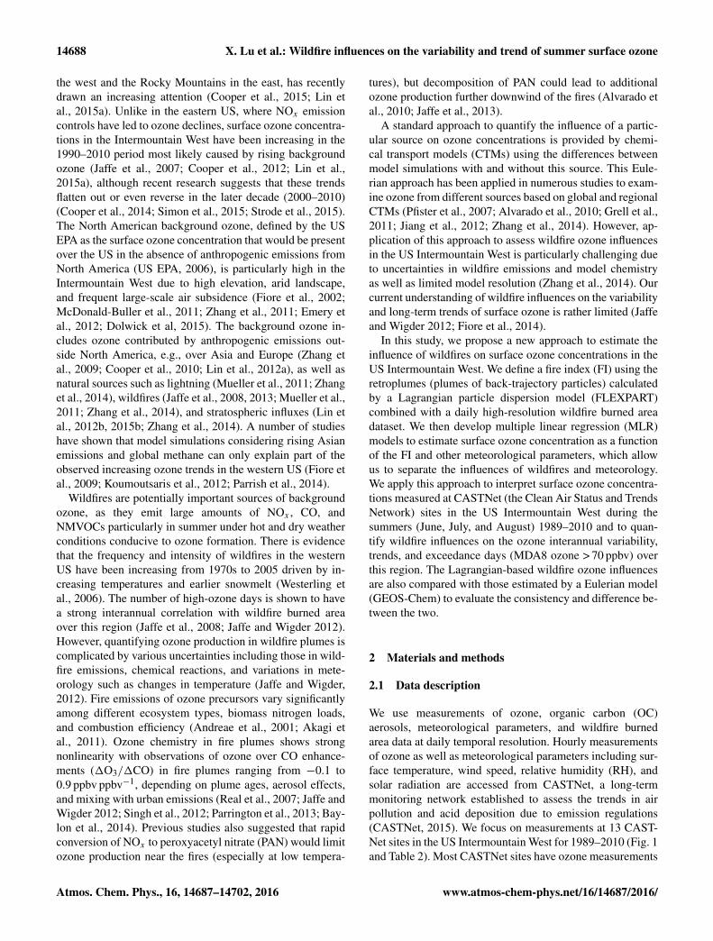
Figure 1. Thirteen CASTNet ozone monitoring sites (Table 2, black pluses) in the US Intermountain West used in this study. Also shown isSLC (Salt Lake City, Utah) urban site (filled triangle). Altitudes of the sites are also labeled. The underlying figure shows terrain elevations(m) of the western US.

for the 22-year period except for (since 1995) Mesa VerdeNational Park (NP) (MEV), Great Basin NP (GRB), Canyon-lands NP (CAN), Big Bend NP (BBE), and (since 2003) Pet-rified Forest (PET). The Yellowstone NP (YEL) site experi-enced monitor relocation in 1996, and we access the 1989–1995 measurements at the earlier YEL site from the NationalPark Service (NPS) following Jaffe et al. (2007) and Cooperet al. (2012).

In addition, we use hourly ozone measurements from 1990to 2010 at the Salt Lake City (SLC; 40.6◦ N, 111.9◦W;1300 m) urban site (Air Quality System, 2015) for compar-ison with the CASTNet background sites and the previouswork of Jaffe et al. (2013). Measurements of OC aerosol arefrom collocated sites of the Interagency Monitoring of Pro-tected Visual Environments (IMPROVE, 2015). OC aerosolconcentrations are 24 h averages measured every 3 days.

We also use the daily wildfire burned area data over NorthAmerica for 1989–2010 developed by Yue et al. (2013) thathas a 0.5◦× 0.5◦ horizontal resolution. This inventory isconstructed using the inter-agency fire reports from the na-tional Fire and Aviation Management Web application sys-tem (FAMWEB, 2014) and applied with a daily scaling fac-tor for the duration of each fire event based on local meteo-rological variables (Yue et al., 2013). The total areas burnedin the Intermountain West range from 90 000 to 2 000 000hectares (ha) in the summers 1989–2010 with a large spatialand interannual variability. This wildfire burned area inven-tory has been used in Zhang et al. (2014) and was able tocapture the episodic enhancements of OC aerosol concentra-

tions measured in the Intermountain West for the summers2006–2008.

2.2 Fire index calculation with the FLEXPART model

Jaffe et al. (2008) previously identified the impacts of wild-fires on ozone at a measurement site using values of monthlywildfire burned area or carbon burned within a certain regionaround the site (e.g., 10◦× 10◦ or 5◦× 5◦). This fire indica-tor generally ignores the variable influence of transport of fireplumes to the site. For instance, a fire downwind of the mea-surement site, even one burning in the immediate vicinity,would not influence the site. Here we propose a new fire indi-cator using 5-day retroplumes simulated by the FLEXPARTLagrangian particle dispersion model and the daily wildfireburned area inventory mentioned above. A retroplume con-sists of a large number of back-trajectory particles that arereleased from a particular receptor location (Cooper et al.,2005). We use FLEXPART version 8.02, which is first de-scribed by Stohl et al. (2005) and has been applied to exam-ine transport of ozone (Cooper et al., 2010) and radionuclidesacross the Pacific Ocean (Stohl et al., 2012). FLEXPARTsimulates the long-range and mesoscale transport, diffusion,and dry and wet deposition of gases or particles (Stohl et al.,2005). It is driven by the National Center for Environmen-tal Prediction (NCEP) Climate Forecast System Reanalysisdata (NCEP CFSR, 2014) with 1-hour temporal resolution,0.5◦× 0.5◦ horizontal resolution, and 37 vertical levels ex-tending from the surface to 1 hPa.

www.atmos-chem-phys.net/16/14687/2016/ Atmos. Chem. Phys., 16, 14687–14702, 2016

14690 X. Lu et al.: Wildfire influences on the variability and trend of summer surface ozone

Table 1. Variables used in the MLR models.

Variable Predictors used in MLR model a Data source

FIs, FIl Fire index for short/long period FLEXPART 5-day backward trajectories andSqrFIs Square root of fire index 0.5◦× 0.5◦ wildfire burned areasSqrFIl

Tsurf Daytime meanb surface temperature CASTNet surface monitoring sites in theWSPsurf Daytime mean wind speed US Intermountain West (http://www.epa.gov/castnet),RH Daytime mean relative humidity for 13 CASTNet sites onlySRAD Daytime mean solar radiation

Tmax Daily maximum temperature NOAA, National Climatic Data Center:AWND Daily average daily wind speed Climate Data Online

(http://www.ncdc.noaa.gov/cdo-web/),for Salt Lake City urban site only

PBLH Gridded daily maximum planetary boundary height NCEP Climate Forecast System Reanalysis (http://rda.ucar.edu/datasets/ds093.0/)

PRCP Gridded daily precipitation Climate Prediction Center of the National WeatherService (ftp://ftp.cpc.ncep.noaa.gov/precip/CPC_UNI_PRCP/GAUGE_CONUS/V1.0/)

U Gridded daily mean 850, 700, 500 hPa zonal wind NCEP/NCAR Reanalysis datasetV Gridded daily mean 850, 700, 500 hPa meridional wind (http://www.esrl.noaa.gov/psd/data/timeseries/daily/)WSP Gridded daily mean 850, 700, 500 hPa horizontal windOme Gridded daily mean 850, 700, 500 hPa vertical velocitySH Gridded daily mean 850, 700, 500 hPa specific humidityHGT Gridded daily mean 850, 700, 500 hPa geopotential heightsT Gridded daily mean 850, 700, 500 hPa temperaturedT Gridded daily mean temperature at 1000mb minus that at 850 hPa

a Units are ◦C (Tsurf, T , dT , Tmax), m s−1 (WSPsurf, WSP, U , V , AWND), % (RH), W m−2 (SRAD), m (PBLH, HGT), kg× kg−1 (SH), 0.1 mm (PRCP) , and pa s−1 (Ome).b Daytime mean represents the average for 10:00–17:00 LT.

For each day at a receptor site, FLEXPART was run inbackward mode, with 250 000 particles released at the sitelocation at a constant hourly rate (∼ 10k particles per hour)during the first 24 h. Previous studies have used the particlesizes of 40 000 (Cooper et al., 2010) and 1 million (Stohlet al., 2012) represent a retroplume. Each particle carries asmall amount of mass decaying with an e-folding time of5 days (mean lifetime of ozone in the Intermountain Westdue to chemical loss and dry deposition as shown in Fiore etal., 2002). Trajectories of these particles are calculated back-wards for 5 days (120 h), together tracing the retroplume ofthe air arriving at the site. The model outputs are in the same0.5◦× 0.5◦ horizontal resolution as the wildfire burned areadata and are hourly residence times of the particles in eachgrid cell. The residence time provides a quantitative mea-sure of the sensitivity of the simulated mixing ratio at thesite location to emission input (Stohl et al., 2003; Seibert andFrank, 2004; Cooper et al., 2010). In total, we have com-puted over 28 000 FLEXPART retroplumes for the 13 Inter-mountain West CASTNet sites and SLC site for the summers1989–2010.

We then define an FI as the product of daily FLEXPARTresidence time integrated from the surface to 5 km and dailywildfire burned area, in unit of s× ha. We use 5 km in thevertical because previous studies have shown that fire emis-sions are occasionally lifted to above the planetary boundarylayer up to 5 km above the surface (Val Martin et al., 2010;Sofiev et al., 2013), and, as shown in Table S1 in the Sup-plement, it provides slightly better correlations with the OCaerosol concentrations than values with 2 km and 2–4 days.The sum of FI over the 5-day period is defined as total fireindex (TFI). The formulas are given as

FI (n)=◦∑

i

∑jEfire(i,j,n)× tr(i,j,n) (1)

TFI=◦∑5

n=1FI(n). (2)

Here Efire(i,j,n) is the wildfire burned area in the model gridcell i (longitude) and j (latitude) on day n, tr(i,j) is FLEX-PART calculated daily residence time as described in detailby Stohl et al. (2003) and Seibert and Frank (2004), and ndefines the backward day in the 5-day period. Figure S1 inthe Supplement shows an example of FI for the site CANon 14 July 2006. In this case, the particles are released on14 July (day n= 1) in the FLEXPART model, and daily res-

Atmos. Chem. Phys., 16, 14687–14702, 2016 www.atmos-chem-phys.net/16/14687/2016/

X. Lu et al.: Wildfire influences on the variability and trend of summer surface ozone 14691

idence time is calculated backwards for 5 days (10–14 July).FI(5) then represents the product of residence time on 10 Julyand wildfire areas burned on that day. TFI as the sum ofFI(1)–FI(5) estimates the total impact of wildfires during the5 days for that site and day.

2.3 Multiple linear regression model

We build MLR models of summer ozone concentrations forthe 13 CASTNet sites and SLC site using FI and meteoro-logical parameters as predictors. This method has been previ-ously used to identify the meteorological factors determiningconcentrations of particulate matter or ozone (Camalier et al,2007; Tai et al., 2010, 2012; Jaffe et al., 2013). Here we usethe metric of daily maximum 8-hour average (MDA8) ozoneconcentration, as it is the regulatory form of the NAAQS. Atotal of 28 meteorological parameters are considered in theMLR models including those measured at surface and fromNCEP data (Tables 1 and 2). Some of these meteorologicalvariables, such as surface temperature, relative humidity, andupper level winds, have been shown before to be correlatedwith surface ozone in the western US (Jacob et al., 2009;Rasmussen et al., 2012; Jaffe et al., 2013).

Wildfire ozone enhancements are sensitive to plume ages.As summarized in Jaffe et al. (2012), 1O3/1CO values inwildfire plumes show distinct differences for plume ages of1–2 days (average 0.018 ppbv ppbv−1) vs. 3–5 days (average0.15 ppbv ppbv−1). Thus instead of using TFI, we separateit to FIs (FI(1)+FI(2)) and FIl (FI(3)+FI(4)+FI(5)) in theMLR models. We also include the square root of FIs and FIl(SqrFIs and SqrFIl) as variables in the regression model to atleast partly account for the nonlinearity of ozone chemistryin wildfire plumes and to narrow the distribution of FI valuesthat are highly episodic. We do not use the natural logarithmform of FI in MLR, because many of the FI values are zero,which would cause invalid values in the regression.

The MLR models can be described as

y = α1×FIs+α2×FIl+β1×SqrFIs+β2×SqrFIl

+

m∑p=1

γp ×metp + c. (3)

Here y is MDA8 ozone concentration, αβγ are the regres-sion coefficients, met denotes the m meteorological param-eters included, and c is the constant term. We then estimateozone enhancements from wildfires and we refer it as MLRwildfire ozone, following

yfire = α1×FIs+α2×FIl+β1×SqrFIs+β2×SqrFIl. (4)

The remaining components define the contribution fromother variables such as meteorology and other sources:

ynofire =

m∑p=1

γp ×metp + c. (5)

To further account for the nonlinear ozone response to wild-fire emissions, we divide the ozone records for each site intothree subsets based on their TFI values: subsets with TFI= 0,with the lower 50 %, and with upper 50 % TFI values (withTFI= 0 excluded). In this way we are able to quantify po-tentially different ozone drivers under high vs. low wildfireconditions. The MLR models as described above are appliedto each subset.

Prior to performing the regression, we calculate correla-tions among ozone and all predictors and remove those fac-tors that show weak correlation with ozone but strong de-pendence on other predictors. To minimize the collinear-ity in the MLR model, we also apply the stepwise regres-sion method; i.e., for each step the model selects the mostpowerful and significant (p< 0.05) predictor explaining theresidual and removes predictors with insignificant influence(p>0.1) (Field et al., 2009). We do not include the inter-action terms to simplify the MLR models. We acknowledgethat including FI and meteorological parameters while ne-glecting their interaction terms in the MLR models inevitablyleads to some degree of collinearity. A measure of it is calledtolerance (calculated as percent of variance in the predictorthat cannot be accounted for by the other predictors) or vari-ance inflation factors (VIF; the inverse of tolerance), withVIF values greater than 10 suggesting a strong collinearity(Field et al., 2009). Our MLR models for all sites (Sect. 3)show tolerable VIF values (< 5), supporting our approach de-scribed above to limit the collinearity.

2.4 The GEOS-Chem model simulations

We further conduct GEOS-Chem model simulations to es-timate wildfire ozone enhancements and to compare withthose from the Lagrangian and statistical approach as de-scribed above. The GEOS-Chem chemical transport modelis driven by the GEOS-5 assimilated meteorological fieldsfrom the NASA Global Modeling and Assimilation Office(GMAO) (http://www.geos-chem.org; v8-02-03) (Bey et al.,2001). We use a nested version of GEOS-Chem that has1/2◦× 2/3◦ horizontal resolution over North America andadjacent oceans (140–40◦W, 10–70◦ N) and 2◦× 2.5◦ overthe rest of the world. We conduct the GEOS-Chem ozonesimulations over North America for 3 years (2006–2008) us-ing the wildfire burned area of Yue et al. (2013). Zhang etal. (2014) have suggested that wildfire NOx emission factorin the standard GEOS-Chem simulation can be too high bya factor of 3. We thus also conduct a sensitivity simulationwith a reduced wildfire NOx emission factor (from 3.0 to1.0 g NO per kg of dry mass burned following Zhang et al.,2014). Wildfire ozone enhancements are computed as dif-ferences between the simulation with all emissions turnedon and a sensitivity simulation with only wildfire emissionsturned off.

www.atmos-chem-phys.net/16/14687/2016/ Atmos. Chem. Phys., 16, 14687–14702, 2016

14692 X. Lu et al.: Wildfire influences on the variability and trend of summer surface ozone

Table 2. Multiple linear regression (MLR) models for summer MDA8 ozone at 13 Intermountain West CASTNet sitesa.

Sitesb R2 (N ) Variables included in the MLR modelc

Glacier NP, MT (GLR, 48◦ N, 113◦W, 976 m) 0.59 (1809) RH, WSPsurf, SRAD, U , V , OME, SH, HGT, T , dT , SH,SqrFIl, SqrFIs,

Yellowstone NP, WY (YEL, 44◦ N, 110◦W, 2400 m) 0.35 (1611) RH, WSPsurf, Tsurf, SRAD, U , V , WSP, Ome, HGT, T , dT ,SH, SqrFIl, SqrFIs, FIl,

Pinedale, WY (PND, 42◦ N, 109◦W, 2388 m) 0.28 (1888) RH, WSPsurf, Tsurf, SRAD, U , V , WSP, Ome, HGT, T , SH,SqrFIl, SqrFIs, FIs,

Centennial, WY (CNT, 41◦ N, 106◦W, 3178 m) 0.19 (1925) RH, U , WSP, HGT, T , SH, SqrFIl, SqrFIs, FIs,Rocky Mtn NP, CO (ROM, 40◦ N, 105◦W, 2743 m) 0.36 (1367) RH, WSPsurf, Tsurf, SRAD, PRCP, U , Ome, T , SH, FIs, SqrFIl,

SqrFIs,Gothic, CO (GTH, 38◦ N, 106◦W, 2926 m) 0.29 (1906) RH, WSPsurf, U , V , WSP, Ome, HGT, T , dT , SH, SqrFIl, FIl,Mesa Verde NP, CO (MEV, 37◦ N, 108◦W, 2165 m) 0.23 (1321) RH, WSPsurf, Tsurf, SRAD, U , V , T , dT , SqrFIl, SqrFIs,Great Basin NP, NV (GRB, 39◦ N, 114◦W, 2060 m) 0.40 (1360) WSPsurf, Tsurf, SRAD, U , WSP, Ome, SH, Ome, HGT, SH,

SqrFIl, SqrFIs, FIs,Canyonlands NP, UT (CAN, 38◦ N, 109◦W, 1809 m) 0.16 (1379) RH, WSPsurf, Tsurf, V , Ome, T , FIl, SqrFIl, SqrFIs,Grand Canyon NP, AZ (GRC, 36◦ N, 112◦W, 2073 m) 0.34 (1912) RH, WSPsurf, SRAD, PRCP, U , V , WSP, Ome, HGT, T , SH,

SqrFIl, FIl,Petrified Forest, AZ (PET, 34◦ N, 109◦W, 1723 m) 0.43 (654) RH, SRAD, V , WSP, Ome, HGT, T , dT , SH, SqrFIlChiricahua NM, AZ (CHA, 32◦ N, 109◦W, 1570 m) 0.50 (1754) RH, SRAD, PBLH, U , V , WSP, HGT, T , dT , SH, SqrFIl, FIl,Big Bend NP, TX (BBE, 29◦ N, 103◦W, 1052 m) 0.46 (1196) RH, WSPsurf, SRAD, U , V , WSP, HGT, T , SqrFIl, SqrFIs, FIl,

FIs

a Coefficients of determination (R2), sample numbers (N), and variables included in the MLR models. b NP is National Park, NM is National Monument, MT is Montana, WY isWyoming, CO is Colorado, NV is Nevada, UT is Utah, AZ is Arizona, and TX is Texas. c Fire index (FIl, FIs), square root of FI (SqrFIl, SqrFIs), and meteorological parametersincluding (1) surface measurements: daytime (10:00–17:00 LT) mean temperature (Tsurf), wind speed (WSPsurf), relative humidity (RH), and solar radiation flux (SRAD); (2)gridded daily precipitation (PRCP); (3) NCEP data at 850/700/500 hPa pressure levels: daily maximum planetary boundary layer height (PBLH), daily mean zonal wind speed (U ),meridional wind speed (V ), horizontal wind speed (WSP), temperature (T ), geopotential height (HGT), vertical velocity (Ome), specific humidity (SH), and temperature at1000 hPa minus that at 850 hPa (dT ). Please refer to Tables 1 and S2 for details on the parameters and MLR models.

3 Model evaluation

We first evaluate our Lagrangian-based FI using its correla-tion to OC aerosol concentrations, as previous studies haveshown that wildfires are an important source of OC aerosolsin the US Intermountain West in summer (Park et al., 2007;Spraklen et al., 2007). As shown in Fig. S2 and Table S1,the TFI values at each CASTNet site are positively corre-lated with OC aerosol concentrations measured at collocatedIMPROVE sites (r = 0.19–0.44). While the TFI vs. OC cor-relations are not very strong, reflecting both uncertainties inthe FLEXPART retroplumes and influence from other OCaerosol sources, the correlations are better (p< 0.01) thanthose with areas burned within 10◦× 10◦ regions. We alsotest the correlations of OC aerosols with FI calculated usingtrajectory residence time at lower altitudes or shorter back-ward time periods, and they in general show slightly weakercorrelations (Table S1).

Table 2 summarizes the predictors included in the MLRmodels and their performance for each CASTNet site withmore details given in Table S2. The MLR models explain 16–59 % of the variability in MDA8 ozone concentration amongthese sites. Figure 2 shows the comparison of measured andMLR predicted ozone concentrations for the ensemble of 13CASTNet sites. The MLR models generally reproduce theozone measurements (R2

= 0.60). These coefficients of de-

termination (R2) are comparable with, or even better than, re-sults simulated by Eulerian CTMs (e.g., R2

= 0.43 in Zhanget al., 2014; R2

= 0.25 in Emery et al., 2012; R2= 0.48 in

Strode et al., 2015) that have limited ability to reproduce themeasured ozone variability in the Intermountain West prob-ably due to the coarse model resolution and complex topog-raphy. However, they are lower than results from Jaffe etal. (2013) or Camalier et al. (2007) that applied the regres-sion models on ozone concentrations at US urban and low-altitude sites.

Jaffe et al. (2013) analyzed the surface ozone concentra-tions measured at the SLC urban site in the western USduring June–September 2000–2012 and showed that a MLRmodel using meteorological variables as predictors could ex-plain 60 % of the MDA8 ozone variation. Here we also ap-plied our MLR models to MDA8 ozone concentrations atSLC in the summers 1990–2010. We find FI and meteoro-logical variables can explain 48 % of the daily MDA8 ozonevariation for summers 1990–2010 (46 % if meteorologicalvariables alone are used and 57 % if September data are alsoconsidered, which explains the higher correlation reported inJaffe et al., 2013), which is a higher value than at most of theCASTNet sites. In addition, as shown in Table 2 and Fig. S3the MLR model R2 values for higher-altitude CASTNet sites(> 2000 m such as CNT, MEV, PND) are generally lowerthan values for lower-altitude sites (such as GLR, CHA, and

Atmos. Chem. Phys., 16, 14687–14702, 2016 www.atmos-chem-phys.net/16/14687/2016/

X. Lu et al.: Wildfire influences on the variability and trend of summer surface ozone 14693

Figure 2. Comparison of the measured versus MLR predictedMDA8 ozone concentrations in the summers 1989–2010 for theensemble of 13 Intermountain West CASTNet sites. The 1 : 1 line(dashed line) and the squared correlation are shown in the inset.

BBE). It appears that the MLR model performs better forUS urban and low-altitude sites than for the CASTNet high-altitude background sites. This is likely because ozone atthe high-altitude CASTNet sites is more affected by regionaltransport from both anthropogenic and natural sources, suchas lightning and stratospheric ozone, and less controlled bylocal meteorology relative to ozone at urban or low-altitudesites.

We find that at the CASTNet sites daytime mean RHis generally the most important predictor. In the low-NOxbackground environment, HOx serves as a strong sink forozone driving the correlation with water vapor concentra-tions (hence RH) (Doherty et al. 2013; Pusede et al., 2015).Fire impacts (FIs and FIl) are included for different sites, aswould be expected by their different travel times from the fre-quent burning areas to the receptor sites. SqrFI often shows ahigher explanatory power than FI, reflecting nonlinear ozoneproduction from wildfire emissions.

We also acknowledge that the MLR models underestimatehigh ozone values especially when measured MDA8 ozoneexceeds 70 ppbv (Fig. 2). These underestimates, however, arenot likely due to model underestimates of wildfire ozone in-fluences. We show in Fig. 3 the relationships of TFI valueswith measured MDA8 ozone, MLR wildfire ozone enhance-ments, and MLR residuals to assess the model performancefor the subset of high ozone days (MDA8 > 70 ppbv). TheMLR model residuals for those high ozone days have littlecorrelation with TFI, and most of the model underestimatesoccur when there are small fire impacts or fires not capturedby the FLEXPART retroplumes. We suggest these underes-timates may be associated with other factors not includedin the statistical model such as transport from Asia or Cal-ifornia, from lightning emissions or stratosphere. These pro-cesses could episodically produce more than 10 ppbv ozonein summer over the US Intermountain West (Zhang et al.,2014).

Figure 3. Evaluation of the MLR model low biases (MLR residu-als) when measured MDA8 ozone concentration exceeds 70 ppbv asindicated in Fig. 2. Scatter plots of total fire index (TFI) versus mea-sured MDA8 ozone (top panel), MLR wildfire ozone enhancements(middle panel), and MLR residuals (bottom panel) are shown. Thecorrelation coefficients are also shown inset.

4 Results

4.1 Consistency and difference with the Eulerian model

It is of particular value to evaluate the MLR wildfire ozoneenhancements with those from the Eulerian approach. Weshow in Fig. 4 such a comparison with the wildfire ozoneenhancements estimated by the GEOS-Chem model in thesummer 2007 when there are large wildfire emissions inIdaho. We can see that the GEOS-Chem model simulatesa sharp gradient of wildfire influences with ozone enhance-ments greater than 20 ppbv over the Idaho and Montana burn-ing areas, which decrease rapidly downwind to 0.5–3 ppbv.

To evaluate the MLR wildfire ozone enhancements, weseparate the 13 CASTNet sites into three groups based ontheir distances to the major burning area in Idaho. As shownin Fig. 4, the MLR and GEOS-Chem estimated wildfireozone enhancements for all three groups are moderatelycorrelated (r = 0.34–0.48, statistically significant p< 0.05),reflecting some consistency between the two approaches.

www.atmos-chem-phys.net/16/14687/2016/ Atmos. Chem. Phys., 16, 14687–14702, 2016

14694 X. Lu et al.: Wildfire influences on the variability and trend of summer surface ozone

GLR

YELPND

CNT ROMGRB GTHCAN MEVGRC PET

CHABBE

Figure 4. Wildfire ozone enhancements over the Intermountain West US in summer 2007. Top panels show the total burned area (upper-left panel) and seasonal mean wildfire ozone enhancements computed by the GEOS-Chem simulation (upper-right panel). Wildfire ozoneenhancements computed by the MLR models are compared with those from the GEOS-Chem simulation. The comparisons are separatedby their distances to the location with the maximum fire emission in Idaho: short-distance sites (bottom-left; GLR, YEL, PND, and GRB),median-distance sites (bottom-middle; CNT, ROM, GTH, CAN, MEV, and GRC), and long-distance sites (bottom-right; PET, CHA, andBBE). Mean wildfire ozone enhancements, correlation coefficients (r), reduced-major-axis regression lines (solid), and 1 : 1 lines (dashed)are shown inset.

There are also considerable differences. We can see thatGEOS-Chem simulates up to 40 ppbv wildfire ozone en-hancements for the short-distance sites, much higher thanthe MLR estimates (mean value of 3.96 ppbv vs. 1.85 ppbv).A sensitivity simulation with a reduced wildfire NOx emis-sion factor (from 3.0 to 1.0 g NO per kg of dry mass burned)would decrease the GEOS-Chem mean ozone enhancementfor the short-distance sites from 3.96 to 2.06 ppbv. In con-trast, for the long-distance sites, the GEOS-Chem wildfireozone enhancements become substantially lower than MLR(0.77 ppbv vs. 1.02 ppbv). We see GEOS-Chem largely over-estimates wildfire ozone influences near the source regionsbut fails to capture continued ozone production in wildfireplumes downwind, as also pointed out by Zhang et al. (2014).It reflects the difficulties for Eulerian models such as GEOS-Chem to simulate wildfire ozone production due to, for ex-ample, missing short-lived VOCs (Jaffe and Wigder, 2012),inadequate PAN chemistry (Alvarado et al., 2010; Fischeret al., 2014), and limiting all fire emissions in the bound-ary layer without considering their injection heights up to thetroposphere (Val Martin et al., 2010; Sofiev et al., 2013). Thelower GEOS-Chem wildfire ozone estimates at those long-distance sites may be also attributed to the model difficulty

in simulating ozone production from small-scale fires nearby.The MLR approach appears to show a more reasonable pat-tern.

4.2 Contribution of wildfires to the MDA8 ozoneconcentration

We use the MLR models to diagnose the influences of wild-fires and other meteorological parameters on MDA8 ozoneconcentrations at the Intermountain West CASTNet sites.Figure 5 shows the scatter plots of observed MDA8 ozoneand MLR predicted ozone at four selected sites located indifferent regions (GLR, ROM, GRB, and CHA). Also shownare the box plots of MLR wildfire ozone enhancements andMLR no wildfire ozone as defined by Eqs. (4) and (5), re-spectively. The MLR models generally reproduce the mea-surements except for high ozone values as we have dis-cussed above. For all the CASTNet sites, the MLR no wild-fire ozone explains most of the measured MDA8 variabil-ity (R2

= 0.10–0.58) compared to MLR wildfire ozone en-hancements (R2

= 0.02–0.12). However, wildfire ozone en-hancements increase as measured MDA8 ozone concentra-tions increase, reflecting higher wildfire impacts on the high-ozone events. We can see in a few cases wildfire ozone

Atmos. Chem. Phys., 16, 14687–14702, 2016 www.atmos-chem-phys.net/16/14687/2016/

X. Lu et al.: Wildfire influences on the variability and trend of summer surface ozone 14695

Figure 5. Scatter plots of observed versus MLR predicted MDA8 ozone concentrations at 4 selected CASTNet sites for the summers 1989–2010. Also shown are the box-and-whisker plots (minimum, 25th, 50th, and 75th percentiles, and maximum) of ozone without wildfireinfluences (blue) and wildfire ozone enhancements (red) for 5 ppbv bins of observed ozone concentrations; both are computed by the MLRmodel as described in the text. The 1 : 1 line (dashed line) and the coefficient of determination (R2) are shown inset.

enhancements reach 10–20 ppbv, causing measured MDA8ozone to approach the ozone quality standard of 70 ppbv.

Another test to separate wildfire ozone influences frommeteorological impacts follows Jaffe et al. (2008), whoshowed ozone concentrations in high fire years were dis-tinctly greater than those in low fire years at the same tem-perature ranges. Here we extend their approach to other me-teorological parameters and to the whole 22-year records.Figure 6 shows the relationships between MDA8 ozone con-centrations and meteorological parameters (daytime temper-ature, wind speed, RH, and solar radiation flux) measured ata Chiricahua National Monument, Arizona (CHA). We com-pare measured MDA8 ozone concentrations with high versuslow wildfire impacts (upper 33 % versus lower 33 % of theTFI values). Meteorological variations have some impacts onboth wildfire activities and MDA8 ozone levels. High wild-fire events are prone to occur with high temperature and so-lar radiation and low RH and wind speed, as indicated bythe number of upper 33 % vs. lower 33 % TFI occurrencesin each increment of meteorological parameters. Ozone con-centrations generally increase with increasing temperatureand decreasing RH. We can also see significant differences(p< 0.05) in the MDA8 ozone concentrations between theupper and lower TFI values for most of the meteorological in-crements. For instance, in the 26–28 ◦C temperature bin, themean MDA8 ozone for the upper 33 % TFI is about 8 ppbv

higher than that for the lower 33 % TFI. This confirms im-pacts of wildfires on ozone that are independent from mete-orological variables.

4.3 Wildfire influences on the ozone interannualvariability and trend

Application of the MLR models to the summers 1989–2010ozone measurements allows us to quantify wildfire influ-ences on the long-term ozone variability and trend. We showin Fig. 7 time series of summer mean measured and MLRpredicted MDA8 ozone concentration for the Intermoun-tain West regional average, as well as for three individualsites (GLR, YEL, and GRC) in the 22 years (1989–2010).The MLR models show good agreements with measurementswith correlation coefficients of 0.85 for the regional averageand 0.52–0.92 for individual sites, but they underestimatethe measured interannual variability. Figure 7 also shows thesummer mean MLR with and without the wildfire ozone,along with the difference between the two. The interannualvariability of surface ozone over the region appears to bemore controlled by the interannual variations of meteorolog-ical parameters, and hence the climate variability, as we cansee that even without wildfire influences, the remaining me-teorological parameters used in the MLR models still predictmost of the interannual variability (MLR no wildfire ozone

www.atmos-chem-phys.net/16/14687/2016/ Atmos. Chem. Phys., 16, 14687–14702, 2016

14696 X. Lu et al.: Wildfire influences on the variability and trend of summer surface ozone

Figure 6. Box-and-whisker plots (minimum, 25th, 50th, and 75th percentiles, and maximum) of observed MDA8 ozone concentrationsfor bins of observed daytime meteorological parameters at CHA site: temperature (upper-left), wind speed (upper-right), relative humidity(bottom-left), and solar radiation flux (bottom-right). MDA8 ozone concentrations are divided by high (TFI at top 33 %, red) and low (TFI atlower 33 %, blue) fire events with the number of occurrences in each bin shown inset. Significant difference (p< 0.05) is marked by asterisks.

Figure 7. Time series of summer mean MDA8 ozone concentrations for the regional averages of eight CASTNet sites with complete 22-yearmeasurements as well as three individual sites. Measurements (black pluses) are compared to the MLR model results (red line). Also shownare the summer mean MLR no wildfire ozone (green line) and MLR wildfire ozone (blue line, right axis). The correlations between measuredand MLR summer means are shown inset.

Atmos. Chem. Phys., 16, 14687–14702, 2016 www.atmos-chem-phys.net/16/14687/2016/

X. Lu et al.: Wildfire influences on the variability and trend of summer surface ozone 14697

vs. MLR ozone r = 0.87–0.99 among individual sites). Thisis further supported by the strong interannual correlations be-tween summer mean MDA8 ozone and meteorological pa-rameters such as daytime mean RH and surface temperatureat individual sites and for the regional averages (r =−0.69for RH, r = 0.48 for temperature), as shown in Fig. S4.

Wildfires contribute 0.3–1.5 ppbv to the summer mean sur-face MDA8 ozone averaged over the Intermountain WestCASTNet sites. In the high fire activity years such as 2003and 2007, the summer mean wildfire ozone enhancementscan reach 3.5 ppbv at the individual sites, e.g., MEV. Theinterannual variability of wildfire ozone enhancements isstrongly correlated with that of the MLR total ozone (r =0.89 for the regional averages and 0.48–0.87 for individualsites). As we can see here, the wildfire-driven interannualvariability (0.3–1.5 ppbv) is much weaker than what can beexplained by meteorological parameters (49.4–53.5 ppbv forthe regional averaged MLR no wildfire ozone). We suggestthat some of the strong correlation between summer meansurface ozone concentrations and wildfire activities reflectstheir common relationships with meteorological parameterssuch as RH and temperature at the interannual scale; e.g.,hot and dry summers would have higher ozone concentra-tions due to stronger photochemistry as well as more wildfireemissions than cold and wet summers (Fig. S4). However,we should acknowledge that ozone production in wildfiresvaries significantly (Jaffe and Wigder, 2012), and the statis-tical models we use here can still underestimate the inter-annual variations of wildfire influences. Better resolving thecauses of variations in wildfire ozone production will help usunderstand the source for interannual variations in ozone.

We further calculate the linear trends of surface ozonein the summers 1989–2010. Figure 8 summarizes the re-sults at three percentile ranges: 93–97th, 48–52th, 3–7thpercentiles at the Intermountain West CASTNet sites. Thethree percentile ranges are used to quantify trends in thelow, median, and high windows of summer MDA8 ozoneconcentration. They also allow us to properly calculate thecorresponding mean wildfire ozone contributions to totalozone by using percentile ranges rather than a single per-centile. We find similar results when using other percentileranges (49–51th or 47–53th). We also show the separatedtrends for the earlier (1989–1999) and later (2000–2010)periods following Strode et al. (2015), who suggested dif-ferent trends in surface ozone for the two periods. Re-gional averaged summer MDA8 ozone concentrations inthe Intermountain West show increasing but statisticallyinsignificant trends of 0.14± 0.21 (p = 0.22), 0.19± 0.21(p = 0.08), and 0.18± 0.20 (p = 0.09) ppbv yr−1 at the93–97th, 48–52th, and 3–7th percentiles, respectively, in1989–2010. Statistically significant (p< 0.05) increasingtrends are found at the YEL (0.42± 0.30 ppbv yr−1) andROM (0.43± 0.39 ppbv yr−1) sites at the median percentiles.These increasing trends primarily occurred in the earlier pe-riod (1989–1999), while nearly all sites show decreasing

ozone trends during 2000–2010. Strode et al. (2015) at-tributed the earlier increasing trends to meteorological vari-ations and the later decreasing trends to domestic emissioncontrols. Our results are consistent with previous studies ofCooper et al. (2012) and Strode et al. (2015), who analyzedthe ozone trends using the same CASTNet measurements butusing the metric of daytime ozone concentration.

Also shown in Fig. 8 are the corresponding ozone trendscontributed by wildfires as estimated by the MLR models.A distinct feature is that the trends of wildfire ozone en-hancements are relatively small but generally in the samedirections as the observed ozone trends. This feature canalso result from meteorological variations that modulate sur-face ozone concentrations and wildfires in similar direc-tions. Most of the sites show increasing wildfire ozone inthe first 11 years (1989–1999) and switch to decreases inthe next 11 years (2000–2010), but only a few of them arestatistically significant. Wildfire ozone enhancements aver-aged over the Intermountain West CASTNet sites increase atrates of 0.02± 0.05 (p = 0.48), 0.02± 0.05 (p = 0.38), and0.03± 0.03 ppbv yr−1 (p< 0.05) at the 93–97th, 48–52th,and 3–7th percentile ranges, respectively, in the summers1989–2010. These values account for about 15 % of the ob-served ozone trends at the same CASTNet sites, representingsmall but important ozone influences from wildfires.

4.4 Wildfire influences on ozone exceedance days

As the ozone air quality standard becomes stricter, it is im-portant to quantify the number of ozone exceedances causedpartly by uncontrollable sources, such as wildfires. We showin Fig. 9 the mean number of days with measured MDA8ozone concentrations exceeding 75, 70, and 65 ppbv aver-aged over the 13 Intermountain West CASTNet sites in thesummers 1989–2010. Also shown is the corresponding num-ber of exceedances that would be present in the absence ofwildfires (estimated as measured ozone minus the MLR wild-fire ozone). We find no statistically significant trends in thenumber of exceedances for both the measured ozone con-centrations and ozone in the absence of wildfires during thesummers 1989–2010.

In the years with poor air quality conditions such as 2002and 2003, there were more than 20 days when MDA8 ozoneexceeds 65 ppbv (accounting for 22 % of the summer days)and about 8 days with MDA8 exceeding 70 ppbv, the currentozone air quality standard. However, if there were no wildfireemissions, the frequency of ozone exceedance days wouldsignificantly decrease. For the total exceedance days at the 13sites in this period, the number with MDA8 above 65 ppbv(above 70 ppbv) would decrease by 28 % to 1509 days (by31 % to 474 days). This reduction is particularly importantin high fire years such as 2002–2003 and 2005–2007 whenone third to half of the exceedances would not occur with-out the fires. In total, wildfires contribute 28, 31, and 32 %of the days when MDA8 ozone exceeds 65, 70, and 75 ppbv,

www.atmos-chem-phys.net/16/14687/2016/ Atmos. Chem. Phys., 16, 14687–14702, 2016

14698 X. Lu et al.: Wildfire influences on the variability and trend of summer surface ozone

Figure 8. Linear trends of summer mean MDA8 ozone concentrations (blue bars, left axis) for 1989–2010 (top panel), 1989–1999 (middlepanel), and 2000–2010 (bottom panel) at eight CASTNet sites and for the Intermountain West regional averages for the (a) 93–97th, (b)48–52th, and (c) 3–7th percentile ranges. Also shown are the trends contributed by wildfire ozone enhancements (red bars, right axis) ascomputed by the MLR models. Statistically significant trends (p< 0.05) are emphasized in dark color.

respectively, reflecting small changes in the relative impor-tance of wildfire influences as lowering the air quality stan-dard over this region.

5 Conclusions

In this study, we have applied a new approach based on a La-grangian particle dispersion model (FLEXPART) and statis-tical models to quantify the wildfire influences on the ozonedaily and interannual variability, trends, and exceedance daysover the US Intermountain West in the summers 1989–2010.The recent implementation of a more stringent ozone stan-dard (70 ppbv) in the United States also motivates the needto better understand contributions and variations of naturalozone sources such as wildfires.

We introduce a FI, a measure of wildfires’ impact at a re-ceptor site, by using 5-day FLEXPART retroplumes (plumesof back-trajectory particles) combined with a daily high-resolution wildfire burned area dataset in the western US.

The FI values are computed for each ozone measurement dayin the summers 1989–2010 for the ensemble of 13 CAST-Net sites and an urban site (SLC) over the US Intermoun-tain West. We then develop statistical MLR models that es-timate MDA8 ozone concentrations at each site as a func-tion of FI and various meteorological variables. We showthat the MLR models explain 60 % (estimated for the en-semble of 13 CASTNet sites) of the variability of MDA8ozone over the US Intermountain West (16–59 % at individ-ual sites), which is comparable with results from current Eu-lerian CTMs (R2

= 0.25–0.48).The MLR models allow us to diagnose the MDA8 ozone

enhancements from wildfires as well as ozone controlledby meteorological variables. We compare wildfire ozone en-hancements estimated by the MLR models with those fromthe GEOS-Chem CTM for summer 2007. While some con-sistency is found as reflected by their moderate correlations(r = 0.34–0.48, statistically significant p< 0.05), the twomethods show rather different patterns. The MLR method ap-

Atmos. Chem. Phys., 16, 14687–14702, 2016 www.atmos-chem-phys.net/16/14687/2016/

X. Lu et al.: Wildfire influences on the variability and trend of summer surface ozone 14699

Figure 9. Mean number of days with MDA8 ozone concentra-tions exceeding the thresholds of 65, 70, and 75 ppbv averaged overthe 13 CASTNet sites in the Intermountain West for the summers1989–2010. The top panel shows the exceedances computed fromthe measurements, and the bottom panel shows results that wouldbe presented in the absence of wildfires (measurements minus theMLR estimated wildfire ozone enhancements).

pears to better capture wildfire ozone influences at larger dis-tances downwind of the fires or ozone produced from small-scale fires. We find that wildfire ozone enhancements esti-mated by the MLR models occasionally reach 10–20 ppbvat the Intermountain West CASTNet sites, and they tend toincrease as measured ozone concentrations increase, reflect-ing higher wildfire impacts on the high-ozone days. Meteo-rological variations also show distinct impacts on both wild-fire activities and MDA8 ozone concentrations. High wildfireevents and high ozone days are often associated with hightemperatures, strong solar radiation, and low RH and windspeed.

We find wildfires increase the summer mean MDA8 ozoneconcentrations by 0.3–1.5 ppbv averaged over the Intermoun-tain West CASTNet sites during 1989–2010. While the inter-annual variability of summer mean wildfire ozone enhance-ments is strongly correlated with that of the MLR total ozone,the wildfire-driven interannual variability is much weakerthan the ozone variability that can be explained by mete-orological parameters. We suggest that the strong interan-nual correlation between summer mean ozone concentrationsand wildfire activities can be partly driven by their com-mon relationships with meteorological parameters such asRH and temperature. These common relationships may also

be responsible for the synchronous trends of summer meansurface MDA8 ozone concentrations and wildfire ozone en-hancements for either the 1989–2010 period or two separated11-year periods (1989–1999 vs. 2000–2010).

Wildfires thus present an important source affecting sur-face ozone air quality in the US Intermountain West. Despitesmall enhancements when averaged seasonally or regionally,they have notable impact on the occurrence of ozone ex-ceedances, reflecting the small-scale and episodic nature ofwildfire emissions. We show that about one third of the sum-mer days (1989–2010) with MDA8 ozone exceeding 70 ppbvwould not occur in the absence of wildfires. A recent study byBrey and Fischer (2016) investigated fire impacts on ozoneat urban sites over the contiguous US and found that fireozone influences can be even higher at locations with highNOx emissions. While we have shown that our Lagrangianand statistical approach provides a quantitative estimate ofozone enhancements from wildfires and can be applied toanalyze long-term ozone records, there are still considerableuncertainties in this approach from both the FLEXPART cal-culation and the MLR models as discussed in the text. Theapproach also does not consider the complexity in fire emis-sions and cannot probe into the physical and chemical pro-cesses in the fire plumes. To address this issue would requiremore detailed fire plume measurements and finer-scale mod-eling approaches, such as imbedding a plume-in-grid modelin CTMs.

6 Data availability

The datasets used in the study can be accessed from websiteslisted in the references or by contacting the correspondingauthor.

The Supplement related to this article is available onlineat doi:10.5194/acp-16-14687-2016-supplement.

Acknowledgements. This work was supported by China’s NationalBasic Research Program (2014CB441303) and by the NationalNatural Science Foundation of China (41475112).

Edited by: Q. ZhangReviewed by: two anonymous referees

References

Air Quality System (AQS), data available at https://www3.epa.gov/airdata/, 2015.

Akagi, S. K., Yokelson, R. J., Wiedinmyer, C., Alvarado, M. J.,Reid, J. S., Karl, T., Crounse, J. D., and Wennberg, P. O.: Emis-sion factors for open and domestic biomass burning for use

www.atmos-chem-phys.net/16/14687/2016/ Atmos. Chem. Phys., 16, 14687–14702, 2016

14700 X. Lu et al.: Wildfire influences on the variability and trend of summer surface ozone

in atmospheric models, Atmos. Chem. Phys., 11, 4039–4072,doi:10.5194/acp-11-4039-2011, 2011.

Alvarado, M. J., Logan, J. A., Mao, J., Apel, E., Riemer, D., Blake,D., Cohen, R. C., Min, K. E., Perring, A. E., Browne, E. C.,Wooldridge, P. J., Diskin, G. S., Sachse, G. W., Fuelberg, H.,Sessions, W. R., Harrigan, D. L., Huey, G., Liao, J., Case-Hanks,A., Jimenez, J. L., Cubison, M. J., Vay, S. A., Weinheimer, A.J., Knapp, D. J., Montzka, D. D., Flocke, F. M., Pollack, I.B., Wennberg, P. O., Kurten, A., Crounse, J., Clair, J. M. S.,Wisthaler, A., Mikoviny, T., Yantosca, R. M., Carouge, C. C.,and Le Sager, P.: Nitrogen oxides and PAN in plumes from borealfires during ARCTAS-B and their impact on ozone: an integratedanalysis of aircraft and satellite observations, Atmos. Chem.Phys., 10, 9739–9760, doi:10.5194/acp-10-9739-2010, 2010.

Andreae, M. O. and Merlet, P.: Emission of trace gases and aerosolsfrom biomass burning, Global Biogeochem. Cy., 15, 955–966,2001.

Baylon, P., Jaffe, D. A., Wigder, N. L., Gao, H., and Hee, J.: Ozoneenhancement in western US wildfire plumes at the Mt. BachelorObservatory: The role of NOx , Atmos. Environ., 109, 297–304,doi:10.1016/j.atmosenv.2014.09.013, 2014.

Bey, I., Jacob, D. J., Yantosca, R. M., Logan, J. A., Field, B. D.,Fiore, A. M., Li, Q., Liu, H. Y., Mickley, L. J., and Schultz,M. G.: Global modeling of tropospheric chemistry with assim-ilated meteorology: Model description and evaluation, J. Geo-phys. Res.-Atmos., 106, 23073–23095, 2001.

Brey, S. J. and Fischer, E. V.: Smoke in the City: How Often andWhere Does Smoke Impact Summertime Ozone in the UnitedStates?, Environ. Sci. Technol., 50, 1288–1294, 2016.

Camalier, L., Cox, W., and Dolwick, P.: The effects of meteorologyon ozone in urban areas and their use in assessing ozone trends,Atmos. Environ., 41, 7127–7137, 2007.

Clean Air Status and Trends Network (CASTNET), data availableat https://java.epa.gov/castnet/clearsession.do, 2015.

Cooper, O. R., Stohl, A., Eckhardt, S., Parrish D. D., Oltmans, S.J., Johnson, B. J., Nédélec, P., Schmidlin, F. J., Newchurch, M.J., Kondo, Y., and Kita, K.: A springtime comparison of tro-pospheric ozone and transport pathways on the east and westcoasts of the United States, J. Geophys. Res., 110, D05S90,doi:10.1029/2004JD005183, 2005.

Cooper, O. R., Parrish, D. D., Stohl, A., Trainer, M., Nédélec, P.,Thouret, V., Cammas, J. P., Oltmans, S. J., Johnson, B. J., Tara-sick, D., Leblanc, T., McDermid, I. S., Jaffe, D., Gao, R., Stith,J., Ryerson, T., Aikin, K., Campos, T., Weinheimer, A., and Av-ery, M. A.: Increasing springtime ozone mixing ratios in the freetroposphere over western North America, Nature, 463, 344–348,2010.

Cooper, O. R., Gao, R., Tarasick, D., Leblanc, T., and Sweeney, C.:Long-term ozone trends at rural ozone monitoring sites acrossthe United States, 1990–2010, J. Geophys. Res.-Atmos., 117,D22307, doi:10.1029/2012JD018261, 2012.

Cooper, O. R., Parrish, D. D., Ziemke, J., Balashov, N. V., Cu-peiro, M., Galbally, I. E., Gilge, S., Horowitz, L., Jensen, N. R.,Lamarque, J. F., Naik, V., Oltmans, S. J., Schwab, J., Shindell,D. T., Thompson, A. M., Thouret, V., Wang, Y., and Zbinden,R. M.: Global distribution and trends of tropospheric ozone:An observation-based review, Elementa: Science of the An-thropocene, 2, 000029, doi:10.12952/journal.elementa.000029,2014.

Cooper, O. R., Langford, A. O., Parrish, D. D., and Fahey, D. W.:Challenges of a lowered US ozone standard, Science, 348, 1096–1097, 2015.

Doherty, R. M., Wild, O., Shindell, D. T., Zeng, G., MacKenzie, I.A., Collins, W. J., Fiore, A. M., Stevenson, D. S., Dentener, F.J., Schultz, M. G., Hess, P., Derwent, R. G., and Keating, T. J.:Impacts of climate change on surface ozone and intercontinentalozone pollution: A multi-model study, J. Geophys. Res.-Atmos.,118, 3744–3763, 2013.

Dolwick, P., Akhtar, F., Baker, K. R., Possiel, N., Simon, H., andTonnesen, G.: Comparison of background ozone estimates overthe western United States based on two separate model method-ologies, Atmos. Environ., 109, 282–296, 2015.

Emery, C., Jung, J., Downey, N., Johnson, J., Jimenez, M.,Yarwood, G., and Morris, R.: Regional and global modeling es-timates of policy relevant background ozone over the UnitedStates, Atmos. Environ., 47, 206–217, 2012.

Field, A.: Discovering Statistics Using SPSS, 3rd Edn. ; Sage Pub-lications: Thousand Oaks, CA, 2009.

Fiore, A. M., Jacob, D. J., Bey, I., Yantosca, R. M., Field, B.D., Fusco, A. C., and Wilkinson, J. G.: Background ozoneover the United States in summer: Origin, trend, and contri-bution to pollution episodes, J. Geophys. Res., 107, D154275,doi:10.1029/2001JD000982, 2002.

Fiore, A. M., Dentener, F. J., Wild, O., Cuvelier, C., Schultz, M.G., Hess, P., Textor, C., Schulz, M., Doherty, R. M., Horowitz,L. W., MacKenzie, I. A., Sanderson, M. G., Shindell, D. T.,Stevenson, D. S., Szopa, S., Van Dingenen, R., Zeng, G., Ather-ton, C., Bergmann, D., Bey, I., Carmichael, G., Collins, W. J.,Duncan, B. N., Faluvegi, G., Folberth, G., Gauss, M., Gong, S.,Hauglustaine, D., Holloway, T., Isaksen, I. S. A., Jacob, D. J.,Jonson, J. E., Kaminski, J. W., Keating, T. J., Lupu, A., Marmer,E., Montanaro, V., Park, R. J., Pitari, G., Pringle, K. J., Pyle, J.A., Schroeder, S., Vivanco, M. G., Wind, P., Wojcik, G., Wu, S.,and Zuber, A.: Multimodel estimates of intercontinental source-receptor relationships for ozone pollution, J. Geophys. Res., 114,D04301, doi:10.1029/2008JD010816, 2009.

Fiore, A. M., Oberman, J. T., Lin, M. Y., Zhang, L., Clifton, O. E.,Jacob, D. J., Naik, V., Horowitz, L. W., Pinto, J. P., and Milly,G. P.: Estimating North American background ozone in US sur-face air with two independent global models: Variability, uncer-tainties, and recommendations, Atmos. Environ., 96, 284–300,2014.

Fire and Aviation Management Web application system(FAMWEB), data available at https://fam.nwcg.gov/fam-web/,2014.

Fischer, E. V., Jacob, D. J., Yantosca, R. M., Sulprizio, M. P., Mil-let, D. B., Mao, J., Paulot, F., Singh, H. B., Roiger, A., Ries, L.,Talbot, R. W., Dzepina, K., and Pandey Deolal, S.: Atmosphericperoxyacetyl nitrate (PAN): a global budget and source attribu-tion, Atmos. Chem. Phys., 14, 2679–2698, doi:10.5194/acp-14-2679-2014, 2014.

Grell, G., Freitas, S. R., Stuefer, M., and Fast, J.: Inclusion ofbiomass burning in WRF-Chem: impact of wildfires on weatherforecasts, Atmos. Chem. Phys., 11, 5289–5303, doi:10.5194/acp-11-5289-2011, 2011.

Interagency Monitoring of Protected Visual Environments (IM-PROVE), data available at http://vista.cira.colostate.edu/improve/, 2015.

Atmos. Chem. Phys., 16, 14687–14702, 2016 www.atmos-chem-phys.net/16/14687/2016/

X. Lu et al.: Wildfire influences on the variability and trend of summer surface ozone 14701

Jacob, D. J. and Winner, D. A.: Effect of climate change on air qual-ity, Atmos. Environ., 43, 51–63, 2009.

Jaffe, D. and Ray, J.: Increase in surface ozone at rural sites in thewestern US, Atmos. Environ., 41, 5452–5463, 2007.

Jaffe, D., Chand, D., Hafner, W., Westerling, A., and Spracklen,D.: Influence of Fires on O3 Concentrations in the Western US,Environ. Sci. Technol., 42, 5885–5891, 2008.

Jaffe, D. A. and Wigder, N. L.: Ozone production from wildfires: Acritical review, Atmos. Environ., 51, 1–10, 2012.

Jaffe, D. A., Wigder, N., Downey, N., Pfister, G., Boynard, A., andReid, S. B.: Impact of Wildfires on Ozone Exceptional Eventsin the Western U. S., Environ. Sci. Technol., 47, 11065–11072,2013.

Jiang, X., Wiedinmyer, C., and Carlton, A. G.: Aerosols from Fires:An Examination of the Effects on Ozone Photochemistry in theWestern United States, Environ. Sci. Technol., 46, 11878–11886,2012.

Koumoutsaris, S. and Bey, I.: Can a global model reproduce ob-served trends in summertime surface ozone levels?, Atmos.Chem. Phys., 12, 6983–6998, doi:10.5194/acp-12-6983-2012,2012.

Lin, M., Fiore, A. M., Horowitz, L. W., Cooper, O. R., Naik, V.,Holloway, J., Johnson, B. J., Middlebrook, A. M., Oltmans, S.J., Pollack, I. B., Ryerson, T. B., Warner, J. X., Wiedinmyer, C.,Wilson, J., and Wyman, B.: Transport of Asian ozone pollutioninto surface air over the western United States in spring, J. Geo-phys. Res.-Atmos., 117, D00V07, doi:10.1029/2011JD016961,2012a.

Lin, M., Fiore, A. M., Cooper, O. R., Horowitz, L. W., Lang-ford, A. O., Levy, H., Johnson, B. J., Naik, V., Oltmans, S.J., and Senff, C. J.: Springtime high surface ozone eventsover the western United States: Quantifying the role of strato-spheric intrusions, J. Geophys. Res.-Atmos., 117, D00V22,doi:10.1029/2012JD018151, 2012b.

Lin, M., Horowitz, L. W., Cooper, O. R., Tarasick, D., Conley, S.,Iraci, L. T., Johnson, B., Leblanc, T., Petropavlovskikh, I., andYates, E. L.: Revisiting the evidence of increasing springtimeozone mixing ratios in the free troposphere over western NorthAmerica, Geophys. Res. Lett., 42, 8719–8728, 2015a.

Lin, M., Fiore, A. M., Horowitz, L. W., Langford, A. O., Oltmans, S.J., Tarasick, D., and Rieder, H. E.: Climate variability modulateswestern US ozone air quality in spring via deep stratosphericintrusions, Nat. Commun., 6, 7105, doi:10.1038/ncomms8105,2015b.

McDonald-Buller, E. C., Allen, D. T., Brown, N., Jacob, D. J.,Jaffe, D., Kolb, C. E., Lefohn, A. S., Oltmans, S., Parrish, D.D., Yarwood, G., and Zhang, L.: Establishing Policy RelevantBackground (PRB) Ozone Concentrations in the United States,Environ. Sci. Technol., 45, 9484–9497, 2011.

Monks, P. S., Archibald, A. T., Colette, A., Cooper, O., Coyle, M.,Derwent, R., Fowler, D., Granier, C., Law, K. S., Mills, G. E.,Stevenson, D. S., Tarasova, O., Thouret, V., von Schneidemesser,E., Sommariva, R., Wild, O., and Williams, M. L.: Troposphericozone and its precursors from the urban to the global scale fromair quality to short-lived climate forcer, Atmos. Chem. Phys., 15,8889–8973, doi:10.5194/acp-15-8889-2015, 2015.

Mueller, S. F. and Mallard, J. W.: Contributions of Natural Emis-sions to Ozone and PM2.5 as Simulated by the Community Mul-

tiscale Air Quality (CMAQ) Model, Environ. Sci. Technol., 45,4817–4823, 2011.

National Center for Environmental Prediction (NCEP) ClimateForecast System Reanalysis (CFSR), data available at http://rda.ucar.edu/pub/cfsr.html, 2014.

Park, R. J., Jacob, D. J., and Logan, J. A.: Fire and biofuel contribu-tions to annual mean aerosol mass concentrations in the UnitedStates, Atmos. Environ., 41, 7389–7400, 2007.

Parrington, M., Palmer, P. I., Lewis, A. C., Lee, J. D., Rickard, A.R., Di Carlo, P., Taylor, J. W., Hopkins, J. R., Punjabi, S., Oram,D. E., Forster, G., Aruffo, E., Moller, S. J., Bauguitte, S. J.-B.,Allan, J. D., Coe, H., and Leigh, R. J.: Ozone photochemistry inboreal biomass burning plumes, Atmos. Chem. Phys., 13, 7321–7341, doi:10.5194/acp-13-7321-2013, 2013.

Parrish, D. D., Lamarque, J. F., Naik, V., Horowitz, L., Shindell,D. T., Staehelin, J., Derwent, R., Cooper, O. R., Tanimoto, H.,Volz-Thomas, A., Gilge, S., Scheel, H. E., Steinbacher, M., andFröhlich, M.: Long-term changes in lower tropospheric baselineozone concentrations: Comparing chemistry-climate models andobservations at northern midlatitudes, J. Geophys. Res.-Atmos.,119, 5719–5736, 2014.

Pfister, G. G., Wiedinmyer, C., and Emmons, L. K.: Impacts of thefall 2007 California wildfires on surface ozone: Integrating localobservations with global model simulations, Geophys. Res. Lett.,35, L19814, doi:10.1029/2008GL034747, 2008

Pusede, S. E., Steiner, A. L., and Cohen, R. C.: Temperature andRecent Trends in the Chemistry of Continental Surface Ozone,Chem. Rev., 115, 3898–3918, 2015.

Rasmussen, D. J., Fiore, A. M., Naik, V., Horowitz, L. W., McGin-nis, S. J., and Schultz, M. G.: Surface ozone-temperature rela-tionships in the eastern US: A monthly climatology for evalu-ating chemistry-climate models, Atmos. Environ., 47, 142–153,2012.

Real, E., Law, K. S., Weinzierl, B., Fiebig, M., Petzold, A., Wild,O., Methven, J., Arnold, S., Stohl, A., Huntrieser, H., Roiger,A., Schlager, H., Stewart, D., Avery, M., Sachse, G., Brow-ell, E., Ferrare, R., and Blake, D.: Processes influencing ozonelevels in Alaskan forest fire plumes during long-range trans-port over the North Atlantic, J. Geophys. Res., 112, D10S41,doi:10.1029/2006JD007576, 2007.

Seibert, P. and Frank, A.: Source-receptor matrix calculation with aLagrangian particle dispersion model in backward mode, Atmos.Chem. Phys., 4, 51–63, doi:10.5194/acp-4-51-2004, 2004.

Shindell, D. T., Lamarque, J. F., Schulz, M., Flanner, M., Jiao, C.,Chin, M., Young, P. J., Lee, Y. H., Rotstayn, L., Mahowald, N.,Milly, G., Faluvegi, G., Balkanski, Y., Collins, W. J., Conley,A. J., Dalsoren, S., Easter, R., Ghan, S., Horowitz, L., Liu, X.,Myhre, G., Nagashima, T., Naik, V., Rumbold, S. T., Skeie, R.,Sudo, K., Szopa, S., Takemura, T., Voulgarakis, A., Yoon, J. H.,and Lo, F.: Radiative forcing in the ACCMIP historical and fu-ture climate simulations, Atmos. Chem. Phys., 13, 2939–2974,doi:10.5194/acp-13-2939-2013, 2013.

Simon, H., Reff, A., Wells, B., Xing, J., and Frank, N.: OzoneTrends Across the United States over a Period of DecreasingNOx and VOC Emissions, Environ. Sci. Technol., 49, 186–195,2015.

Singh, H. B., Cai, C., Kaduwela, A., Weinheimer, A., and Wisthaler,A.: Interactions of fire emissions and urban pollution over Cali-

www.atmos-chem-phys.net/16/14687/2016/ Atmos. Chem. Phys., 16, 14687–14702, 2016

14702 X. Lu et al.: Wildfire influences on the variability and trend of summer surface ozone

fornia: Ozone formation and air quality simulations, Atmos. En-viron., 56, 45–51, 2012.

Sofiev, M., Vankevich, R., Ermakova, T., and Hakkarainen, J.:Global mapping of maximum emission heights and resultingvertical profiles of wildfire emissions, Atmos. Chem. Phys., 13,7039–7052, doi:10.5194/acp-13-7039-2013, 2013.

Spracklen, D. V., Logan, J. A., Mickley, L. J., Park, R. J.,Yevich, R., Westerling, A. L., and Jaffe, D. A.: Wildfiresdrive interannual variability of organic carbon aerosol in thewestern US in summer, Geophys. Res. Lett., 34, L16816,doi:10.1029/2007GL030037, 2007.

Stevenson, D. S., Young, P. J., Naik, V., Lamarque, J. F., Shindell,D. T., Voulgarakis, A., Skeie, R. B., Dalsoren, S. B., Myhre, G.,Berntsen, T. K., Folberth, G. A., Rumbold, S. T., Collins, W. J.,MacKenzie, I. A., Doherty, R. M., Zeng, G., van Noije, T. P. C.,Strunk, A., Bergmann, D., Cameron-Smith, P., Plummer, D. A.,Strode, S. A., Horowitz, L., Lee, Y. H., Szopa, S., Sudo, K., Na-gashima, T., Josse, B., Cionni, I., Righi, M., Eyring, V., Conley,A., Bowman, K. W., Wild, O., and Archibald, A.: Troposphericozone changes, radiative forcing and attribution to emissions inthe Atmospheric Chemistry and Climate Model Intercompari-son Project (ACCMIP), Atmos. Chem. Phys., 13, 3063–3085,doi:10.5194/acp-13-3063-2013, 2013.

Stocker, T. F., Qin, D. ; Plattner, G. -K., Tignor, M., Allen, S. K.,Boschung, J., Nauels, A., Xia, Y., Bex, V., and Midgley, P. M.:IPCC, 2013: Climate change 2013: The physical science basis.Contribution of working group I to the fourth assessment reportof the intergovernmental panel on climate change; CambridgeUniversity Press, Cambridge, United Kingdom and New York,NY, USA, 2013.

Stohl, A., Forster, C., Eckhardt, S., Spichtinger, N., Huntrieser, H.,Heland, J., Schlager, H., Wilhelm, S., Arnold, F., and Cooper,O.: A backward modeling study of intercontinental pollutiontransport using aircraft measurements, J. Geophys. Res., 108,D124370, doi:10.1029/2002JD002862, 2003.

Stohl, A., Forster, C., Frank, A., Seibert, P., and Wotawa, G.: Tech-nical note: The Lagrangian particle dispersion model FLEX-PART version 6. 2, Atmos. Chem. Phys., 5, 2461–2474,doi:10.5194/acp-5-2461-2005, 2005.

Stohl, A., Seibert, P., Wotawa, G., Arnold, D., Burkhart, J. F., Eck-hardt, S., Tapia, C., Vargas, A., and Yasunari, T. J.: Xenon-133 and caesium-137 releases into the atmosphere from theFukushima Dai-ichi nuclear power plant: determination of thesource term, atmospheric dispersion, and deposition, Atmos.Chem. Phys., 12, 2313–2343, doi:10.5194/acp-12-2313-2012,2012.

Strode, S. A., Rodriguez, J. M., Logan, J. A., Cooper, O. R., Witte, J.C., Lamsal, L. N., Damon, M., Van Aartsen, B., Steenrod, S. D.,and Strahan, S. E.: Trends and variability in surface ozone overthe United States, J. Geophys. Res.-Atmos., 120, 9020–9042,2015.

Tai, A. P. K., Mickley, L. J., and Jacob, D. J.: Correlations betweenfine particulate matter (PM2.5) and meteorological variables inthe United States: Implications for the sensitivity of PM2.5 toclimate change, Atmos. Environ., 44, 3976–3984, 2010.

Tai, A. P. K., Mickley, L. J., Jacob, D. J., Leibensperger, E. M.,Zhang, L., Fisher, J. A., and Pye, H. O. T.: Meteorological modesof variability for fine particulate matter (PM2.5) air quality inthe United States: implications for PM2.5 sensitivity to climatechange, Atmos. Chem. Phys., 12, 3131–3145, doi:10.5194/acp-12-3131-2012, 2012.

US Environmental Protection Agency: Air Quality Criteria forOzone and Related Photochemical Oxidants (Final), Vols. I, II,and III, EPA 600/R-05/004aF-cF, 2006.

US Environmental Protection Agency: National ambient air qualitystandards for ozone, Fed. Regist., 80, 65292–65468, 2015.

Val Martin, M., Logan, J. A., Kahn, R. A., Leung, F. -Y., Nel-son, D. L., and Diner, D. J.: Smoke injection heights from firesin North America: analysis of 5 years of satellite observations,Atmos. Chem. Phys., 10, 1491–1510, doi:10.5194/acp-10-1491-2010, 2010.

Westerling, A. L., Hidalgo, H. G., Cayan, D. R., and Swetnam,T. W.: Warming and Earlier Spring Increase Western US ForestWildfire Activity, Science, 313, 940–943, 2006.

Yue, X., Mickley, L. J., Logan, J. A., and Kaplan, J. O.: Ensembleprojections of wildfire activity and carbonaceous aerosol concen-trations over the western United States in the mid-21st century,Atmos. Environ., 77, 767–780, 2013.

Zhang, L., Jacob, D. J., Kopacz, M., Henze, D. K., Singh, K., andJaffe, D. A.: Intercontinental source attribution of ozone pollu-tion at western US sites using an adjoint method, Geophys. Res.Lett., 36, L11810, doi:10.1029/2009GL037950, 2009.

Zhang, L., Jacob, D. J., Downey, N. V., Wood, D. A., Blewitt, D.,Carouge, C. C., van Donkelaar, A., Jones, D. B. A., Murray, L.T., and Wang, Y.: Improved estimate of the policy-relevant back-ground ozone in the United States using the GEOS-Chem globalmodel with 1/2◦× 2/3◦ horizontal resolution over North Amer-ica, Atmos. Environ., 45, 6769–6776, 2011.

Zhang, L., Jacob, D. J., Yue, X., Downey, N. V., Wood, D. A., andBlewitt, D.: Sources contributing to background surface ozonein the US Intermountain West, Atmos. Chem. Phys., 14, 5295–5309, doi:10.5194/acp-14-5295-2014, 2014.

Atmos. Chem. Phys., 16, 14687–14702, 2016 www.atmos-chem-phys.net/16/14687/2016/