Who Benefits from Kindergarten? Evidence from the ... · Who Benefits from Kindergarten? Evidence from the Introduction of State ... system occurred in all 50 ... representing enrollment

Who Benefits from Kindergarten? Evidence from the Introduction of State Subsidization

(Job Market Paper)

Elizabeth Dhuey

Department of Economics University of California, Santa Barbara

January 2007

Abstract

Over the last seventy years, all states in the U.S. began to publicly subsidize kindergarten using state revenue. The variation in adoption dates across states allows for a unique opportunity to measure the effectiveness of the largest early education program implemented in recent history. The significant, immediate increase in the availability of kindergarten within a state is used to identify the effect of enrollment in kindergarten. The estimated effects from the instrumental variables specification indicate that kindergarten decreases later grade failure by 64 percent. In addition, the present study examines what types of children benefit from the increased availability of kindergarten using a reduced form model. Black children and children of low socioeconomic status benefit the most from the increased availability of kindergarten. Black children with access to kindergarten are 27 percent less likely to fail a grade in school and earn wages 4 percent higher as adults. Children of the poorest quartile of parents are 35 percent less likely to fail a grade. Overall, kindergarten has a significant and positive effect on academic and labor market outcomes primarily for black individuals and those who grow up in a lower socioeconomic status. I would like to thank my advisor, Peter Kuhn, and my committee members, Kelly Bedard and Jon Sonstelie, for the help and suggestions. I would also like to thank Olivier Deschenes and Cathy Weinberger for their helpful comments.

1

1. Introduction

Over the last 70 years, a massive adoption of kindergarten in the public primary school

system occurred in all 50 states in the U.S. This resulted in a dramatic increase in the availability

of early childhood education. Recently, there has been a renewed push to increase the prevalence

of early childhood education programs by such means as publicly provided full-day kindergarten

or universal preschool. This paper hopes to shed light on the likely effects of these recent

initiatives by examining the effect of the large-scale implementation of kindergarten programs in

the middle of the last century. In particular, this study assesses how attending kindergarten

benefits students and, more specifically, what types of children benefit from attendance. Do boys

benefit more than the girls? Black children more than white children? Poor more than rich? In

addition to determining who benefits from attending publicly supported kindergarten, this paper

also estimates the magnitude of the effect.

Frederick Froebel formed the first kindergarten in Germany in 1837. The curriculum

emphasized socialization and readied children for primary education. The kindergarten

movement later expanded to the United States, taking root in Wisconsin nineteen years later.

Over the next several decades, many towns and cities started offering kindergarten. Initially, all

kindergarten funding came from either private or local sources such as local philanthropic

organizations, private tuition payments, or local tax dollars. However, between 1935 and 1986,

all U.S. states transitioned to subsidizing kindergarten using state revenue. This enabled states to

provide kindergarten as a part of their public primary school educational system. In most states,

this subsidization enabled a public school to count kindergarten students as a part of their

enrollment for the purposes of calculating state aid. In other cases, the district or school was

given additional state money in the form of a grant or appropriation for providing kindergarten.

This decreased the districts’ costs of providing kindergarten, thus increasing its availability. Ohio

was the first state to subsidize kindergarten in 1935. The rest of the country followed and began

subsidizing kindergarten during the next fifty years. Mississippi was the last state to join the

movement when it began subsidizing kindergarten with state revenue in 1986.

Very few researchers have examined the educational or labor market effects of

kindergarten attendance. Cascio (2004) uses a similar methodology to this paper to look at the

average effect of kindergarten enrollment in Southern and Western states. She finds that, on

2

average, state funding of kindergarten decreases the probability that a child repeats a grade by 2

percentage points but that it had no effect on the rate of high school dropouts. Using the Current

Population Survey, she finds some evidence that minority children benefit more than non-

minority children. Spiess, Büchel and Wagner (2003) examine the effects of attending

kindergarten in Germany. They find no significant relationship between kindergarten attendance

and later school track placements for children of native German households. However, they find

that children of immigrant households do benefit in terms of track placements from attending

kindergarten.

Additionally, the evidence is mixed regarding the benefits of full-day kindergarten as

opposed to half-day kindergarten. Clark and Kirk (2000) survey the literature and find diverse

results. Much of the recent research finds a small positive effect on academic achievement and

behavior (see DeCicca (2006), Fusaro (1997), and Walston & West (2004)). However, there are

also many researchers who find no difference in later academic achievement between full-day

and half-day kindergarten attendance (Karweit (1992)). Cannon, Jacknowitz and Painter (2004)

find that full-day kindergarten increases behavior problems for boys but that it also increases

math scores for girls. Unfortunately, many of these studies on kindergarten efficacy rely on small

sample sizes that are neither representative nor adequate as to the size of their control groups.

The literature regarding preschool and earlier childhood education and intervention

programs is much larger than that for kindergarten. Currie (2001) reviews the economics

literature and finds that programs such as Head Start and closely related preschool and early

school enrichment programs have significant short and medium-term benefits and that the effects

are usually greater for disadvantaged children.1 Gormley and Gayer (2003) examine a newly

implemented pre-kindergarten program in Oklahoma and find that the program increased

cognitive/knowledge scores, motor skill scores, and language scores for Hispanic and black

children but had little impact on white children. A recent paper by Baker, Gruber and Milligan

(2005) examines the introduction of universal childcare in Quebec in the late 1990’s. They

conclude that the children were actually worse off by becoming more hostile, possessing less

motor and social skills, and tending to become ill more often.

1 Ludwig and Miller (2007) use a regression discontinuity approach and find significant benefits of Head Start in terms of decreased mortality rates. Currie and Neidell (2007) find that when Head Start spending was higher, children attending Head Start have higher reading and vocabulary scores.

3

Although state subsidization of kindergarten began in all states between 1935 and 1986,

the largest increase in state sponsored kindergarten occurred between 1960 and 1980. Therefore,

this study uses policy changes between 1960 and 1980 to evaluate the effectiveness of state

sponsored kindergarten. The effect of state-sponsored kindergarten can be isolated by comparing

cohorts before and after state subsidization was introduced assuming that outcomes for each

cohort would be the same except from the effect of kindergarten attendance.

This study uses data for the entire United States to estimate the effect of kindergarten

enrollment on future academic and labor market outcomes. More specifically, the impact of state

sponsored kindergarten can be examined across four dimensions by exploring differences in (1)

how boys and girls respond, (2) how children of different races are affected, (3) how children of

different socioeconomic status respond, and (4) how children of different ages are affected. The

paper focuses on the following outcomes: grade failure, educational attainment, and labor market

outcomes, such as wages and employment status. The evidence shows that attending

kindergarten decreases the probability that a child fails a grade and increases the probability that

a child finishes high school and becomes employed. There is little evidence of gender differences

in reduced grade failure rates and some evidence that children of relatively different ages are

affected differently due to kindergarten availability. However, large differences appear in grade

failure between white and black children and between children of different socioeconomic

statuses. More specifically, black children’s failure rate is decreased by about 27 percent while

white children benefit by about 15 percent. Consistent with this difference, the hourly wage rate

for black children increases by about 4 percent later in life. The biggest gap between groups is

between socioeconomic groups. The poorest children are about 26-35 percent less likely to fail a

grade after the introduction of state funded kindergarten, while there is no effect on the failure

rate of rich children.

2. Econometric Model

A. Cohort Level – Two Stage Least Squares

Ideally, one can estimate the effect of kindergarten attendance on future academic and

labor market outcomes using individual-level data on kindergarten enrollment and outcome

measures. This relationship can be estimated using the following equation:

stitsstististi TSXEY εβββ +++++= 21 (1)

4

where stiY denotes the outcome measure, such as grade failure, educational attainment or a labor

market outcome, for individual i in state s and birth year t. stiE is an indicator variable

representing enrollment in kindergarten. stiX is the vector of controls, sS are state fixed effects

and tT are birth year fixed effects.

The coefficient 2β measures the causal impact of attending kindergarten on the outcome

measure. The causal interpretation depends on the assumption that 0]|[E =stististi XE ε . However,

kindergarten enrollment is not mandatory for most children and hence probably not random.

Currently only eight states require children to enter school at age 5. Compulsory schooling does

not start until age 6 in the remaining forty-two states. In addition, kindergarten enrollment was

not random prior to becoming subsidized at the state level due to the fact that it was privately or

locally funded. Therefore, this assumption does not hold. It is not clear in which direction the

bias will occur. For example, communities that provided kindergarten before state subsidization

were probably wealthier than communities without kindergarten. In addition, students who

attended kindergarten by paying tuition would have generally been wealthier than non-attending

children.2 These children might be less likely to fail a grade or have better labor market

outcomes regardless of kindergarten. Therefore, estimating equation (1) may lead to upward

biased estimates of the effect of kindergarten enrollment. However, it was also the case that

kindergarten was used by some organizations to socialize and “Americanize” immigrant children

(Spodek, 1988). Kindergarten was used to help immigrant children by providing food and

clothing, in addition to education in some areas (de Cos, 1997). In this case, it may be that

equation (1) would be biased downward because these children may have been more likely to

fail a grade or have worse labor market outcomes, holding everything else constant. Regardless

of the direction of bias, random enrollment did not exist, and therefore ordinary least squares

estimates will be biased, and an instrumental variables strategy should be employed.

Unfortunately, individual level data on kindergarten enrollment and data regarding

academic and labor market outcomes do not exist from one source. However, data regarding

state/cohort level kindergarten enrollment figures do exist in the Digest of Education Statistics

and data on academic and labor market outcomes are available in the U.S. Census.3 Equation (1)

2 Cascio (2005) finds that these children had more highly educated mothers and came from smaller families. 3 See Section 3A for more details regarding the kindergarten enrollment and the Census data.

5

can be estimated by aggregating the data regarding outcomes to the state/cohort level and

merging this data with the aggregated enrollment data.

Instrumental variables estimates of equation (1) can be calculated by using the state

subsidization of kindergarten ( stK ) as an instrument for state-level kindergarten enrollment.

More specifically, stK is a dummy variable that indicates whether the state subsidized

kindergarten during a particular year. The start of state subsidies created a large increase in

kindergarten availability for almost all children in the state. This increased the probability that

any particular child attended kindergarten. Using an estimation technique similar to Imbens and

van der Klaauw (1995) and Angrist (1991), this paper uses variation in state/cohort level

aggregate enrollment rates, stE produced by policy changes to estimate the effect of enrolling in

kindergarten. Figure 1 illustrates the percentage of five year olds enrolled in kindergarten. It

displays the aggregated percentage of five year olds enrolled in kindergarten in the 27 states that

began to subsidize kindergarten between 1960 and 1980. The largest increase occurs, about a 25

percentage point increase, between the year before the start of state subsidization and the year

after the start of state subsidization.

The following first stage equation can be estimated as a part of a two stage least squares

estimation strategy. The first stage equation can be written as:

sttsststst vTSXKE +++++= δδδ 21 (2)

where stE is the percentage of 5 year olds enrolled in kindergarten for each state for each birth

year and stK is an indicator variable that equals 1 if a state subsidized kindergarten in a

particular year and 0 otherwise. The vector, stX , includes the state/birth year level mean values

for the control variables. For completeness, the cohort level second stage can be written as:

sttsststst TSXEY εβββ +++++=∧

21 (3)

where stE∧

are the predicted values from equation (2). Therefore, using the instrumental variables

approach 2β can be calculated, which estimates the effect of enrolling in kindergarten on future

outcomes on children that are induced to attend due to state subsidization.

The two stage least squares estimate imposes the following non-testable exclusion

restriction: 0]|[E =ststst XK ε . If policy makers began to subsidize kindergarten due to other

6

factors that affect academic and labor market outcomes, the estimates for kindergarten could not

be disentangled from those changes. However, most of the large changes in education programs

came in the form of federal policy enacted during this time period, including the introduction of

Title I of the Elementary and Secondary Education Act of 1965, and would have impacted all the

states at the same time and therefore would be captured by the year fixed effects. Even though

the previous assumption is non-testable, a number of state level policies regarding education that

changed at the same time as kindergarten subsidization can be help constant because they may

also affect academic and labor market outcomes. State Supreme Court rulings on the

constitutionality of school-finance systems and school finance litigation information4 can be used

as control variables. The first wave of school finance litigation occurred in California in the

1970s beginning with the landmark case Serrano v. Priest. Most states experienced some type of

school litigation within the next twenty-five years. However, only five states had challenges to

their school-finance system within a five-year window of the beginning of kindergarten

subsidization. These states are Arizona, Montana, Georgia, Idaho and Oregon. Including these

changes as controls does not affect the results or conclusions of this paper.

Aside from policies, other time-varying factors might exist that could be correlated with

student outcomes. More specifically, within-state changes in the laws affecting kindergarten

need to be uncorrelated with other state-specific changes that might affect student outcomes.

However, the results are similar if state-specific cohort linear or quadratic time trends are

included.5

B. Individual Level – Subgroups

Much of the early childhood literature finds clear differences in the effect of early

childhood interventions on children of different genders and socioeconomic statuses (Currie

(2001)). Therefore, it is important to examine whether this is also true for kindergarten

enrollment. Because kindergarten enrollment data is only available at the state/cohort level for

the cohorts affected by the changes in subsidization, the above instrumental variables estimate

cannot be calculated for subgroups because the enrollment data are not available in a

disaggregated form. Therefore, I specifically examine how different groups of individuals are

4 This information was collected from Murray, Evans, and Schwab (1998) and the National Center for Education Statistics at http://nces.ed.gov/edfin/litigation/index.asp. 5 These results are available from the author upon request.

7

affected by the availability of state sponsored kindergarten using a reduced form approach using

individual level data.

The reduced form allows the estimation of the average effect of increased availability of

kindergarten on future outcomes. The following regression is run separately for boys and girls.

stitsstististi wTSXKY +++++= γγγ 21 (4)

Figure 1 demonstrates the average increase of 25 percentage point gain due to the state funding

of kindergarten. However, it may be the case that different states had different proportions of

children enrolled in kindergarten before and after state subsidization. These differences could be

due to differences in availability due to local or private funding but it also could be due to the

difference in timing. States that begun to subsidize kindergarten at a later time than other states

might have more children enrolled due to increasing trends in enrollment. These differences

between states change the marginal group of children who are induced to attend kindergarten due

to the increased availability. More concretely, Figure 2 displays the percentage of five year olds

enrolled in the two largest states that began subsidizing kindergarten during the 1960’s and

1970’s: Texas and Florida. Panel A depicts the change in kindergarten enrollment in Texas five

years before and after kindergarten became state funded in 1967. In 1967, the first year of

kindergarten subsidization by the state, enrollment increased dramatically. Approximately 15

percent of five year olds were enrolled in kindergarten before it became state subsidized. Five

years after state subsidization, approximately 85 percent of five year olds were enrolled. This

corresponds to about a 70-percentage point increase. A slightly different pattern is observed in

Florida in Panel B. The Florida data show a more gradual increase of kindergarten enrollment.6

Before state subsidization, only about five percent of five year olds were enrolled in

kindergarten. Five years after state subsidization, sixty percent of five year olds were enrolled.

This translates into a 55 percentage point increase. The marginal children in Texas, who are the

children that are induced to attend kindergarten due to the increased availability and decreased

cost, might be significantly different than the marginal children in Florida. Therefore, the

interpretation of 2γ is the average effect of the increased availability of kindergarten for all the

changing states.7

6 Excluding observations right around the official year of change does not change the conclusions of this paper. 7 Restricting the sample to states that have similar levels of five year olds enrolled in kindergarten before or after state subsidization or restricting the sample to states that have similar percentage point increase due to state subsidization does not substantially change the results or conclusions of this paper.

8

The effect of kindergarten on different groups of children can be estimated by interacting

a control variable with the indicator for state sponsored kindergarten. For example, the

differences in kindergarten effectiveness between black children and white children are

estimated using the following regression.

stitsstistististististi wTSXBBKKY +++++×++= γγγγγ 4321 (5)

Where stiB is an indicator for the black students and stisti BK × is the interaction between the

dummy variable for state subsidized kindergarten and the dummy variable for black children.

Therefore, 3γ is the average differential effect of kindergarten availability on black students. stiX

represents the vector of controls. sS are fixed effects for birth state and tT are fixed effects for

birth year.8 All standard errors are clustered at the state level and are heteroskedastic-consistent.9

3. Data and Descriptive Statistics

A. Data Sources

The primary data source used in this study is the U.S. Census. Section 4 examines grade

failure, the short-term outcome. It uses the 1 percent sample from the Form 2 state, metro, and

neighborhood files from the 1970 U.S. Census. These samples make up a 3 percent sample of the

United States in 1970. This data is merged with the 5 percent sample from the 1980 Census. The

sample is restricted to individuals from these two Census years who are ages 6 to 15 years old,

and were born in the United States. Section 5 expands the analysis to include longer run

outcomes such as educational attainment and labor market outcomes. This analysis uses the 5

percent sample from the 2000 U.S. Census and restricts the sample to individuals between the

ages of 25 and 50 who were born in the United States.

Kindergarten enrollment data is from the Biennial Survey of Education, later known as

the Digest of Education Statistics. Due to the absence of data in 1956, 1958, 1960, 1962, and

8 It is important to include controls for birth year or age since each individual has a different window of time depending on their age for completing the outcome measure. An alternative approach would be to use a hazard model. 9Even though it is possible to run the previous reduced form models using more aggregated data, the individual level data is used when examining the effect of kindergarten availability on subgroups. The aggregation of the data to the subgroup/state/cohort level has the potential of creating very few or no observations in particular cells. However, all results are similar. There is no change in interpretation if the data is aggregated to the subgroup/state/cohort level.

9

1964 these enrollment rates are linear interpolations.10 The kindergarten enrollment in year t and

the first grade enrollment in year t+1 were used to construct an enrollment ratio that

approximates the enrollment rate for kindergarten in each year, t.

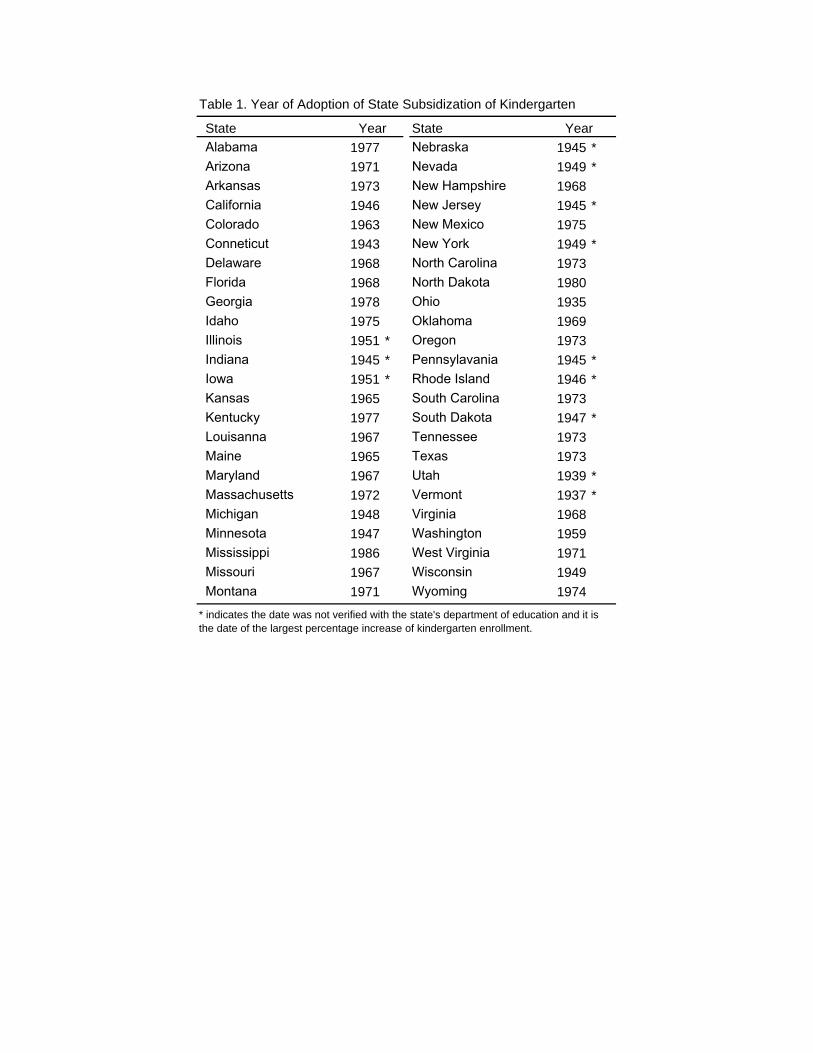
The date in which each state began funding kindergarten as a part of its public primary

school education system at the state level was gathered by contacting each state’s education

department. Some of these dates were verified using information collected by Cascio (2004),

Tanner and Tanner (1975) and Steiner (1972). Table 1 lists the year in which kindergarten first

began to be subsidized using state revenue. I am unable to obtain the exact year of the beginning

of state funding for twelve states. A star in Table 1 designates these states. It has been confirmed

that these states all began to subsidize kindergarten using state money before 1960.11 The date

listed in Table 1 for the starred states is the year in which there was the largest increase in

kindergarten enrollment. This analysis will focus on the time period from 1960 and 1980, where

27 states began subsidizing kindergarten. Therefore, the unconfirmed dates for these twelve

states will not affect the analysis, as they did not began subsidizing kindergarten during the

1960’s or 1970’s.

This study uses both short run and long run measures of effectiveness or benefit. The first

outcome measure concerns whether the student failed a grade in school.12 An indicator measure

of whether the child is below grade for her age is used as a proxy for failure or grade repetition.

This measure is constructed from the Census data using the child’s age and grade level and the

state’s cutoff date for kindergarten entry. If a child is below the grade level they should be in for

their age, they are considered retained or failed. For instance, if a child should be seven years old

in second grade but a seven year old is observed in first grade, that child is considered retained.

This retention measure includes individuals whose school entry was delayed by their parents as

well as individuals who failed a grade and were retained by their teachers. Therefore, the

available data cannot disentangle children who failed and children who entered schooling late.13

This measure is still valid as long as the rules about failing and parents’ tendency to hold back

their children do not change at the same time as the introduction of subsidies. Fortunately, there 10 Kindergarten enrollment data is missing for select states in select years. The results of the analysis does not change if these data are also linearly interpolated. 11 See Turner and Turner (1975) and/or Steiner (1972). 12 Cascio (2005) and Oreopoulos, Page, and Stevens (2006) both use this proxy as a measure of educational achievement. 13 Cascio (2005) examines the validity of using this proxy and finds that the misclassification attenuates regression coefficients by 35% when the proxy is an outcome using Current Population Survey data.

10

is no evidence that rules regarding failure have changed or that overall standards regarding

failing within the public school system have increased over time (Roderick, 1994). In addition,

parent’s behavior regarding entry should not change because kindergarten is not compulsory in

most states. If parents did respond at the same time as the policy change, they should be more

likely to hold back their children because the children would be starting school at an earlier age.

If this occurred it would bias the estimates downwards.

There is extensive literature documenting the association between grade retention and

poor later educational outcomes.14 Roderick (1994) reports a large association between being

retained and dropping out of high school. Jacob and Lefgren (2002) show that the immediate

consequence of being retained is increased academic performance, but that there is no effect on

later math scores and a negative effect on reading scores. This paper also uses longer run

academic outcome measures, such as the educational attainment of an individual, and labor

market outcomes such as wages, time spent working and employment status.

B. Descriptive Statistics

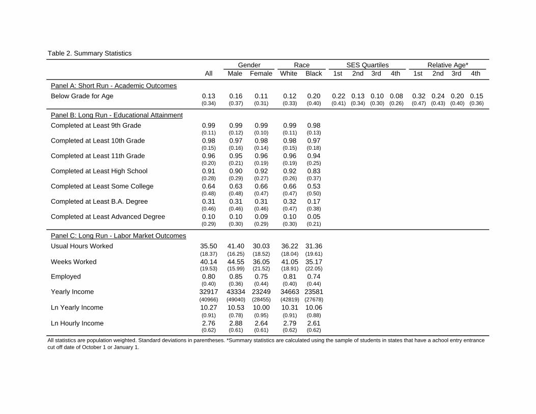
Table 2 displays the summary statistics for the outcome measures by different groupings.

The first outcome measure listed is the fraction of a cohort below grade for age, the proxy for

grade failure. The mean value for individuals ages 6-15 is 13 percent. Males are 5 percent more

likely to have repeated a grade than females. Black students are 8 percent more likely to be

below grade than white students. The poorest quartile of students, the first quartile, is almost

three times more likely to be below grade for their age than the richest quartile of students, the

fourth quartile. The last grouping of individuals is by relative quarters of birth.15 Children who

are the relatively youngest, quarter 1, are approximately twice as likely to be behind a grade than

children who are the relatively oldest, quarter 4.

Panel B and C display the statistics for the longer run outcome measures studied in this

paper: educational attainment and labor market outcomes. These statistics are not broken up by

SES quartiles or relative age quarters because the information does not exist regarding an

individual’s socioeconomic status as a student or her quarter of birth in the data.16 Therefore, the

14 See Holmes (1989) for a review of the literature. 15 These statistics are for children born in states in which the cutoff is either October 1st or January 1st, the only cutoff dates in which a relative age measure can be perfectly assigned. See section 4E for more details. 16 The 2000 U.S. Census does not contain the variable quarter of birth.

11

SES and relative age measures can not be established. Panel B focuses on the longer run

academic measures. Females are more likely to make it to 9th, 10th, and 11th grade, become high

school graduates, and attend college but are only slightly more likely to earn a B.A. degree.

Black individuals are less likely than white individuals to have completed all the long run

academic outcomes. Panel C includes six labor market outcomes: usual hours worked, usual

weeks worked, whether the individual is employed, yearly income, ln of yearly income, and ln of

hourly wage. Overall, males and white individuals have higher values in all six categories than

females and black individuals, respectively.

4. Results – Grade Failure

A. Cohort Level – Two Stage Least Squares

The analysis begins by estimating the ordinary least squares, first stage, and two stage

least squares models for the short run outcome variable, below grade for age, using the aggregate

state/cohort level data. Table 3 contains these results. 17 Column 1 includes the coefficients from

equation 1 with the outcome variable being the below grade for age indictor variable. The noisy

point estimate of -1.4 indicates that there might be a negative relationship between kindergarten

enrollment and failure rates. However, as discussed in Section 2, this OLS relationship may be

biased due to correlation between the unobservable variables and kindergarten enrollment rates.

Column 2 contains the results from the first stage estimation strategy from equation 2.

The introduction of state funding of kindergarten increases the kindergarten enrollment rate by

about 25 percentage points. The F-statistic associated with the instrument in the first stage

equation is 32. This indicates that state subsidization of kindergarten used as an instrument does

not suffer from the weak instrument problem (Staiger and Stock (1997)).

The two stage least squares result is in column 3. These estimates can be interpreted as

the local average treatment effect of the enrollment in kindergarten. The estimate pertains to the

children who were induced to attend kindergarten due to the decrease in cost. The point estimate

of -0.083 indicates that public kindergarten attendance decreases the probability of failure by 8.3

percentage points. This relationship is statistically significant at the five percent level and

translates into a 64 percent reduction in repeating a grade. It is also worth noting that this

17 Fixed effects for age, in addition to birth year, are included in regressions that use both the 1970 and 1980 Census.

12

estimate is larger than the point estimate found by Cascio (2004), but her sample is significantly

smaller and is disaggregated by race.

B. Reduced Form by Gender

The results from the preceding section show a statistically significant negative

relationship between attending kindergarten and failing a grade in school. These results are

consistent with the literature regarding kindergarten but only answer the question about the

average effectiveness of kindergarten. Much of the literature regarding preschool has shown that

very specific groups of children are affected the most by early education interventions.18

Therefore, it is important to examine which children specifically benefit from the introduction of

kindergarten into the public primary school system. By using the reduced form analysis and by

estimating equation 4, these issues can be investigated.

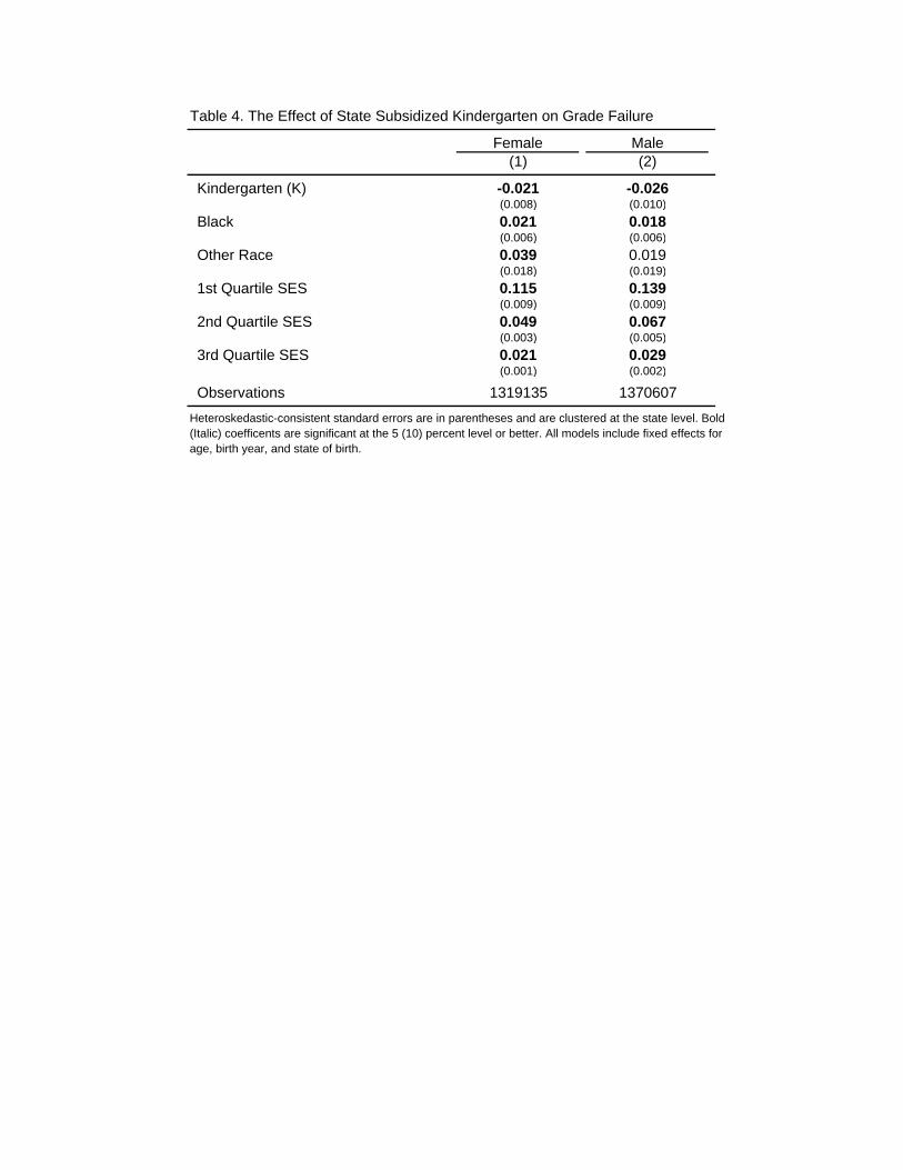
Table 4 reports the most basic results for the reduced form specifications. Column 1

displays the results for the female subsample. The coefficient on kindergarten indicates that the

introduction of kindergarten into the public primary school educational system decreases failure

rates by 2.1 percentage points. This translates into a 20 percent decrease in the failure rate. The

results for the male subsample are similar. The introduction of state funded kindergarten

decreases retention rates by 2.6 percentage points, which translates into a 17 percent decrease.

The difference between boys and girls is not statistically significant. This is an interesting

finding because conventional wisdom and previous literature find differences between boys and

girls in terms of effects of early childhood education (Cannon, Jacknowitz and Painter, 2004).

Using this metric, there is little evidence of this.

The IV estimates of Table 3 specifically measures the effect of enrolling in kindergarten

on grade failure for the group of children who were induced to attend kindergarten due to state

subsidization. These reduced form estimates can be interpreted as the average effect of

increasing kindergarten availability by state subsidization on grade repetition. The instrumental

variable estimates should always be larger in magnitude than the reduced form estimates since

the first stage estimate will be a positive fraction.

18 See Cannon, Jacknowitz and Painter (2004), Currie (2001), Gormley and Gayer (2003) and Spiess, Büchel and Wagner (2003).

13

C. Reduced Form by Race

I next explore the possibility that children of different races are affected differently by the

introduction of state subsidized kindergarten. In this case, the sample is limited to children who

are either white or black. The dummy variable of whether the child is black is interacted with the

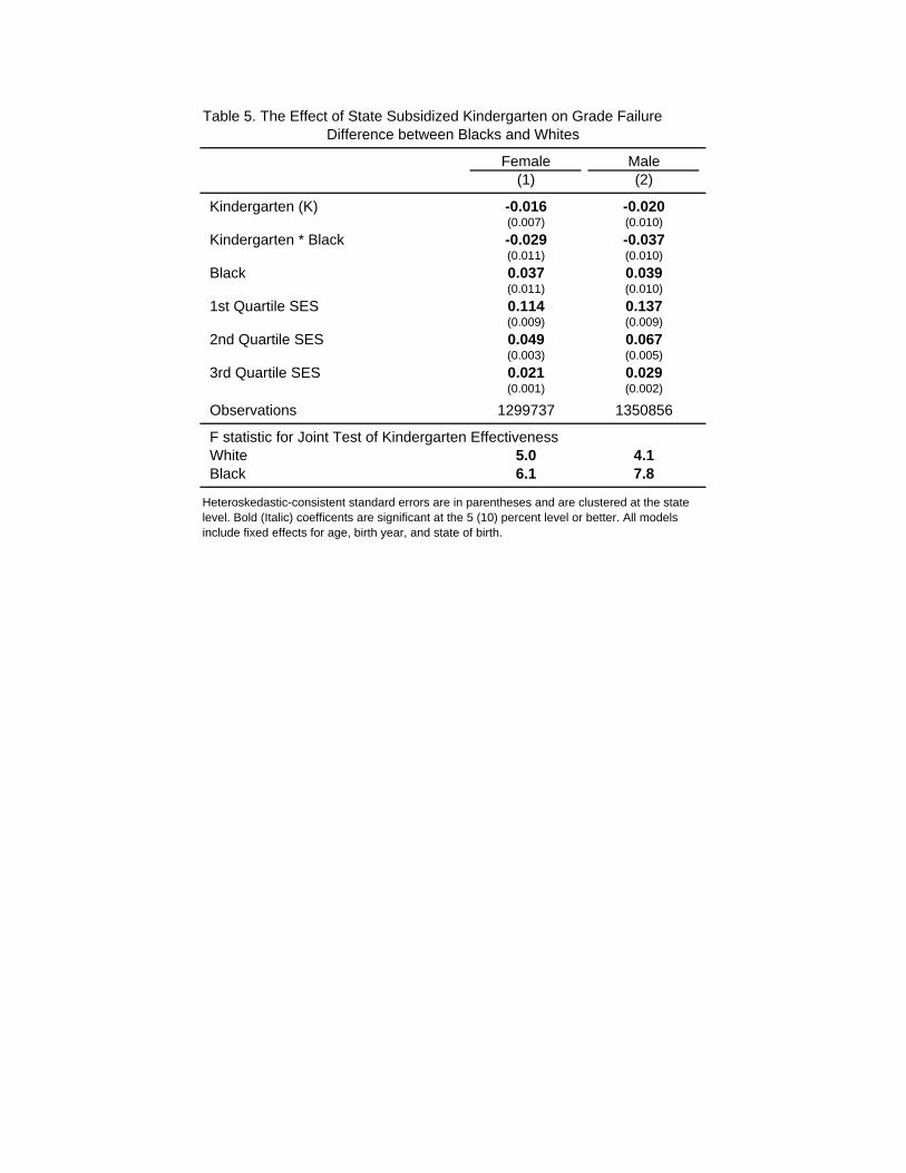
dummy variable for state sponsored kindergarten. Table 5 reports the coefficient for kindergarten

( 2γ ) and the coefficient for the interaction of kindergarten and black ( 3γ ) from equation 5. The

results for females are reported in column 1. White females’ failure rate decreased about 1.6

percentage points, a 17 percent decline. However, the black females’ failure rates decreased

about 4.5 percentage points, a 28 percent decline. The difference between the black and white

females is statistically significant at the five percent level. The bottom of the table reports the F

statistic for the joint significance of kindergarten effectiveness. For the black female, this is the F

statistic of the joint test of significance for both the coefficient on kindergarten and the

coefficient on the interaction between black and kindergarten.

The introduction of publicly funded kindergarten decreased the failure rates for white

males by about 2 percentage points, which translates into a 14 percent decrease. However, black

males are significantly more likely to have a reduction in failure rates. Their failure rates

decrease by 5.7 percentage points, or 26 percent. This is a large and statistically significant

difference.

There is significant evidence that children of different races are affected differently by

the introduction of kindergarten into public school. This difference may be caused by the

alternative situations children of different races face when kindergarten is not subsidized. If a

child has access to high quality childcare in the absence of subsidized kindergarten, kindergarten

attendance may not be as beneficial for that child.

D. Reduced Form by SES

A greater benefit to children of lower socioeconomic status has been noted in previous

research. Head Start and the pre-K program in Oklahoma have both shown the most effect on

children of lower socioeconomic statuses (Currie (2001) and Gormley and Gayer (2003)).

Section 4C focuses on racial differences in the effectiveness of the introduction of publicly

funded kindergarten, while holding socioeconomic status constant. This section will examine the

different effects of kindergarten on children of different socioeconomic statuses.

14

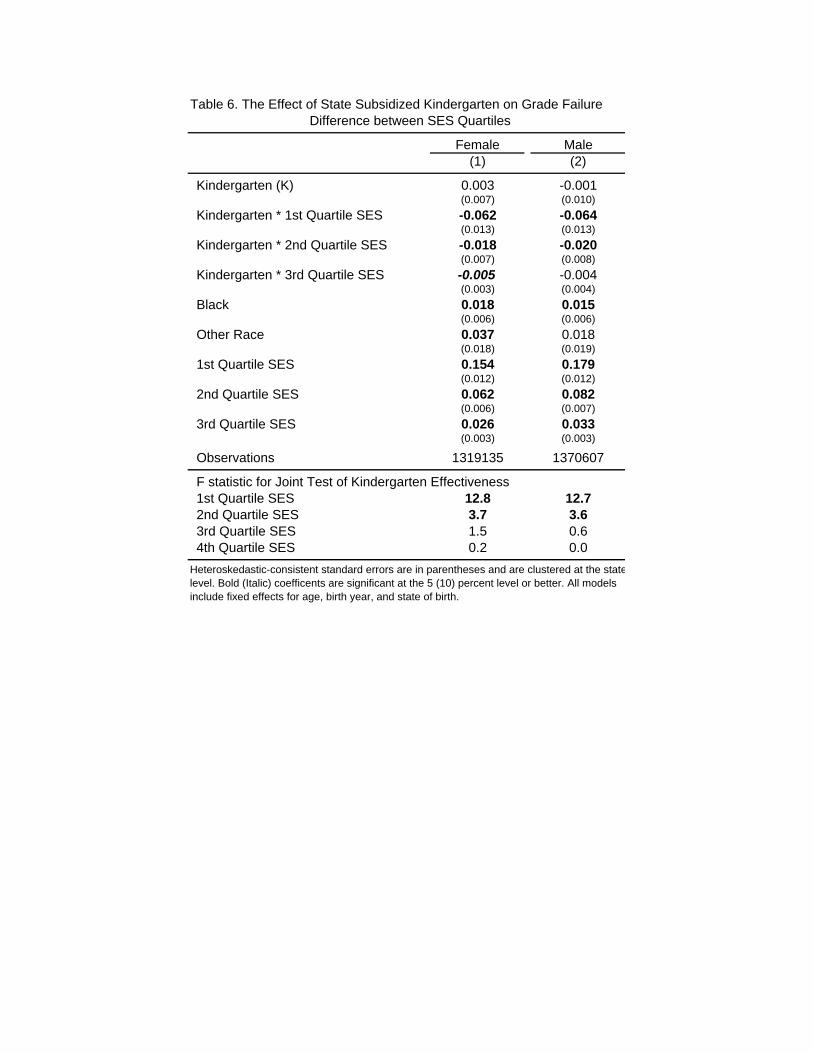
Table 6 explores the relationship between socioeconomic status and kindergarten

effectiveness. Indicator variables of which quartile of the socioeconomic distribution that each

student belongs to is constructed by using the poverty measure in the Census. The 1st quartile

corresponds to the poorest children while the 4th quartile corresponds to the richest children.

These indicators of SES quartile are interacted with the indicator for kindergarten to measure the

varying effect of the increased availability of state sponsored kindergarten on children of

different SES groups. The omitted category in the regression is the children of the 4th quartile,

the richest children. Column 1 once again displays the results for females. The introduction of

state subsidized kindergarten only affects quartiles 1 through 3. Quartile 1, the poorest children,

has a large and significant coefficient. The introduction of state funded kindergarten decreases

the failure rate by 5.9 percentage points, or 35 percent. The second quartile is also statistically

significantly impacted at the five percent level, with a 1.5 percentage point, or 18 percent

decrease. The F statistics for quartiles 3 and 4 are not statistically significant at the five or ten

percent level. Column 2 of Table 6 examines the effect on males and finds similar results. Only

the poorest two quartiles of SES were affected by the introduction of state sponsored

kindergarten. The poorest quartile is 6.5 percentage points, or 26 percent, less likely to fail

whereas the second quartile students are 2.1 percentage points, or 13 percent less likely to do so.

The richest two quartiles show no effect. Figure 2 graphically depicts the relationship between

SES quartiles and the reduction of retention rates. Two stars indicate joint statistical significance

at the five percent level. Panel A displays the results for the females and Panel B displays the

results for the males. Once again, there is very little difference between the males and females.

E. Reduced Form by Relative Age

The final grouping of students is between children of dissimilar relative ages. There is a

rich vein of literature discussing at what age children are ready to enroll in kindergarten or the

appropriate age for beginning school.19 However, a child’s absolute age is not the only factor in

determining her success in kindergarten and beyond. A child’s age relative to her classmates may

matter in terms of how much benefit that child receives from early childhood education.

Recently, economists have shown that the relatively oldest children in a grade are more likely to

(1) score higher on standardized math and science exams, (2) become high school leaders, (3)

19 See de Cos (1997) for a thorough review of literature pertaining to kindergarten readiness.

15

take college entrance exams, and (4) attend university immediately after high school.20 It is

important to examine the effects of a child’s relative age in relation to the benefits of

kindergarten enrollment.

The state’s cutoff date and individual’s quarter of birth are used to construct a measure of

relative age (Q) for each individual. The state’s cutoff date was collected using historical state

statutes and session laws. Given an absence of information regarding a statewide cutoff date in

some states, no accurate measure of relative age can be assigned. Therefore, missing values are

assigned to these children. If statewide cutoff data exists, the relative measure is constructed as

follows: Q1 = 1 for students born in the last quarter of the calendar year, which would make

them the relatively youngest students prior to the cut-off; and Q1 = 0 otherwise. Q2, Q3, and Q4

are similarly defined for each subsequent quarter of birth. For example, using an October 1st

cutoff, children born between July 1 and September 30 are the youngest (Q1 = 1), while children

born between October 1 and December 31 are the oldest (Q4 = 1).

Ideally, the data would contain each individual’s birth date. However, due to data

restrictions, only the quarter of birth of the individual is provided. Therefore, this study only uses

the quarter of birth measure for states that have a cutoff date of either January 1 or October 1.

Other cutoff dates are inaccurate in assigning the relative age measure because it is unclear

which children are relatively the oldest or youngest. For instance, if the cutoff date is November

1, children born in the last quarter of the year may either be the relatively youngest (if they are

born in October) or the relatively oldest (if they are born in November or December).

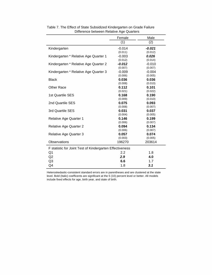
Table 7 reports the coefficient from the interaction of the relative quarter of birth

measures with the indicator variable for state sponsored kindergarten. The results for female

students are reported in column 1 and displayed graphically in Figure 3, Panel A. The results

show a downward pattern from a 2.6 percentage point decline for relative quarter 2 to a 1.7

percentage point decline for the oldest, relative quarter 4. However, the relatively youngest

students are affected at a magnitude similar to the relatively oldest students.

The results for males reported in column 2 and displayed in Figure 3, Panel B show a

similar pattern. The point estimates indicate that the introduction of kindergarten into the public

primary school increases the failure rate for the relatively youngest males and decreases the

failure rate between 2 and 3 percentage points for the other three quarters with a declining

20 See Bedard and Dhuey (2006), Datar (2003), Dhuey and Lipscomb (2005), and Fredriksson and Öckert (2004).

16

pattern between relative quarter 2 and relative quarter 4. The coefficients in this section are not

estimated very precisely. This is mainly due to the decreased sample size since the analysis can

only use states that have a cutoff date of January 1st or October 1st. The coefficients are

essentially of the same magnitude but are more precisely estimated if the boys and girls are

pooled together in the analysis.

The patterns observed meet expectations, given the previous literature regarding relative

age effects. The relatively youngest children are often at a disadvantage in terms of academic

outcomes. Kindergarten attendance may level the playing field since it emphasizes socialization

and school readiness, the very areas in which the relatively youngest are disadvantaged.

However, the increase in failure rates for the relatively youngest males and the small magnitude

of the results for the females is surprising.

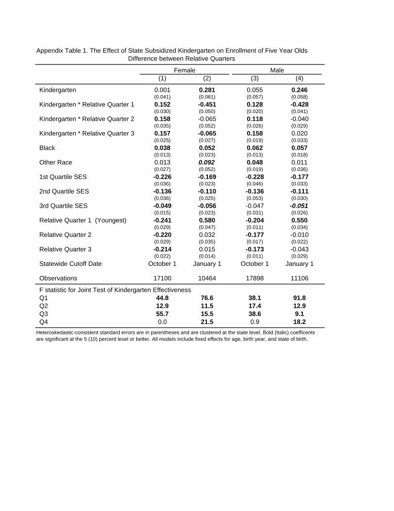
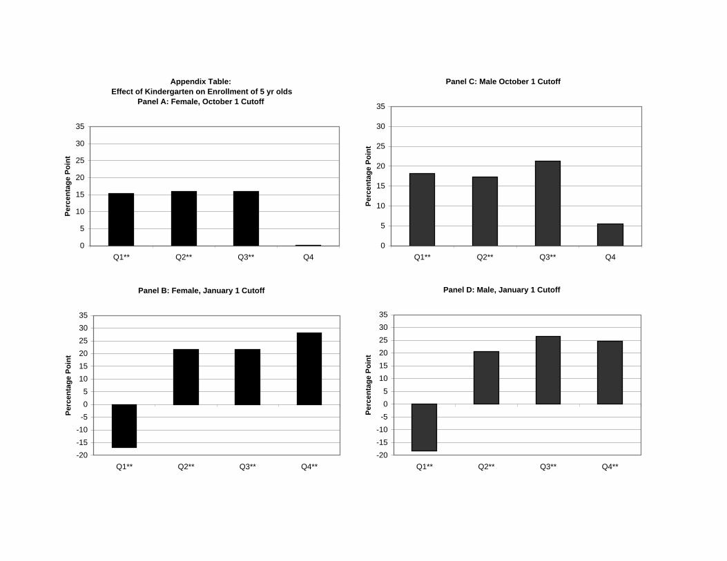
The enrollment behavior of 5 year olds before and after state-funded kindergarten is

examined because the positive or smaller results for the youngest boys and girls may be due to

selection into kindergarten. Appendix Table 1 reports the results from the analysis using the

same independent variables as before but uses an indicator for whether the child is enrolled in

school as the dependent variable. This analysis uses only five year olds in the fall of 1959, 1969,

and 1979 from the 1960, 1970, and 1980 Census. The analysis is run separately for males and

females and for the January 1 and October 1 cutoff dates. The enrollment patterns of children

with different relative ages are quite different and can be seen graphically in Appendix Figure 1.

The difference in starting age makes a large difference in parental enrollment decisions.

The measure of below grade for age is a proxy for failure rates since it is unable to

disentangle whether a child has failed a grade or whether the child’s parents purposely delayed

entry for that child. It has been shown that the parents have purposely delayed entry for children

of the relatively youngest quarter in states that have a cutoff of January 1. Therefore, the

estimates of the effective reduction of retention rates by relative quarter underestimate the effect

for the relatively youngest quarter.

Despite the significant effects that relative age has on academic outcomes, there is less

evidence that it influences the benefit the child receives from kindergarten enrollment. The

relatively youngest students do seem to benefit more than the relatively oldest children but this

comparison is small in relationship to the black/white difference or the difference in

socioeconomic status. This explanation may be related to the previous one regarding alternative

17

childcare options when kindergarten is not available or is too expensive. Childcare options are

not related to a child’s relative age; therefore, a child’s relative age may have little impact on the

effectiveness of kindergarten outside the increased socialization and school readiness that

kindergarten provides.

5. Results – Long Run Outcomes

A. Cohort Level - Two Stage Least Squares

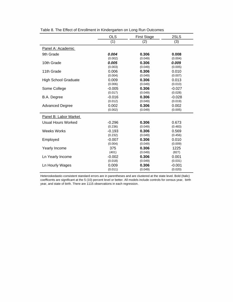
The remainder of the paper focuses on longer run outcomes. Table 8 reports the results

for all equations of interest for the longer run outcome variables. Column 1 reports the OLS

result for the impact of enrollment in kindergarten on the outcome variable. Column 2 displays

the coefficient 2δ from the first stage estimated by equation (2). Lastly, column 3 shows the two

stage least square estimates for 2β , using the introduction of state subsidization of kindergarten

as an instrument for kindergarten enrollment.

The only statistically significant results obtained using the collapsed state/cohort level

data are the first stage result and the results for 9th and 10th grade completion. The first stage

coefficient is a 30.6 percentage point increase in the enrollment after state funded kindergarten is

introduced and is tightly estimated. Column 3 coefficients indicate that enrolling in kindergarten

will increase 9th and 10th grade completion by almost 1 percentage point. The point estimates for

all other outcome variables are too noisy to interpret.

B. Reduced Form by Gender

The earlier results on grade repetition indicate that there are large differences in the

benefit from kindergarten between subgroups which may hold true for longer run outcomes.

Once again, the kindergarten enrollment data can not be disaggregated. Hence, the reduced form

specification is used to estimate the average effect of increased kindergarten availability on

different groups of individuals.

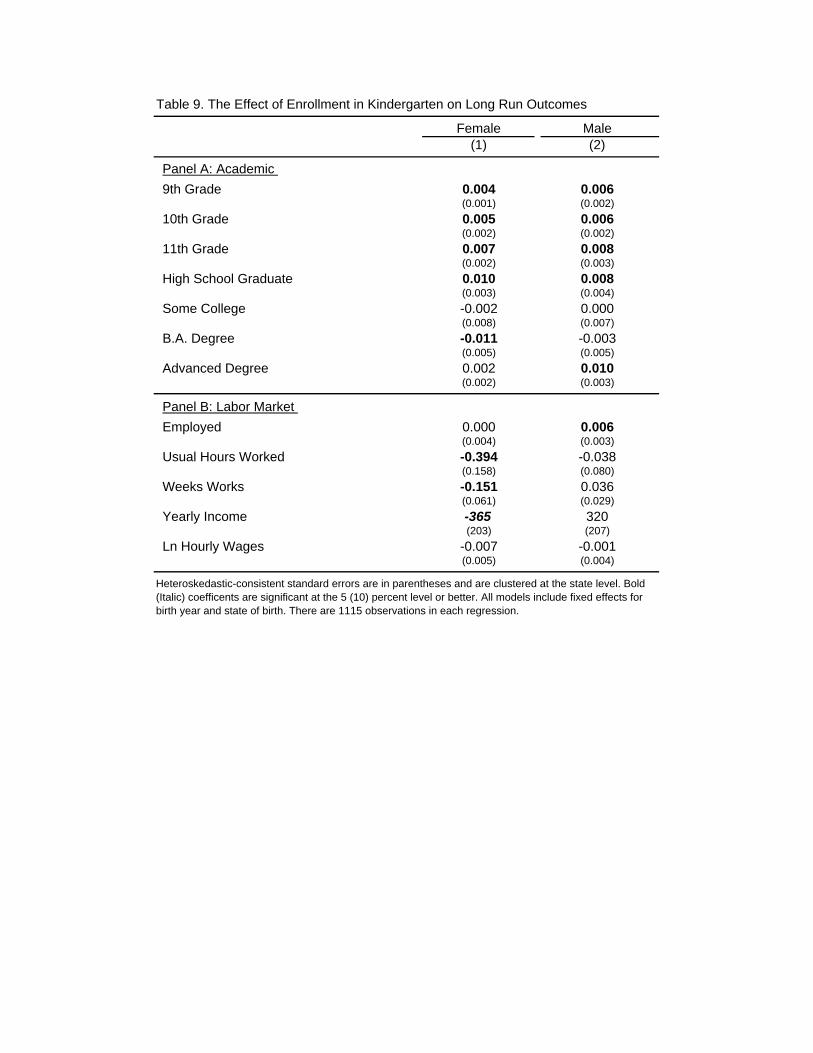
Table 9 reports the results from the reduced form equation (4) using the individual-level

data for the long run academic outcomes by gender. The coefficient reported is 2γ from equation

4. Column 2 reports the results for the male sample. The longer run academic outcomes are in

Panel A. There are positive and statistically significant effects of kindergarten availability on all

the academic outcome variables except for college attendance and college graduation outcomes.

18

The point estimate indicates that the increase of availability due to the introduction of

kindergarten into the public primary school system increases high school graduation rates by 0.8

percentage points. Similar results are reported for 9th grade through 11th grade completion rates.

The increase in availability of kindergarten increases high school graduation by about 8 percent.

Panel B reports a statistically significant and positive result for employment status but no other

results are significant. The educational attainment results for the female sample reported in

column 1 are similar in magnitude to those of the males. However, the female results contain a

puzzling outcome, indicating that after kindergarten becomes state funded, female students are

less likely to earn a B.A. degree. The labor market outcome measures are reported for the sample

of women but these results should be interpreted cautiously due to many changes in the women’s

labor market during this time period. Overall, there are three significant results, usual hours,

usual weeks worked, and yearly income which are negative. Therefore, there are some effects on

school completion rates and labor market outcomes due to the increase of kindergarten for both

males and females.

B. Reduced Form by Race

Table 10 reports the point estimates for the indicator variable for kindergarten and the

interaction between the indicator variable for black and the indicator variable for kindergarten

from equation (5) using the long run outcome measures as the dependent variable. Panel A

reports the results from the male sample whereas Panel B reports the results from the female

sample. Columns 1 through 4 report point estimates similar to Table 9 but with slightly less

precision in the high school graduate model in the male sample. The interaction variable between

black and kindergarten is not statistically significantly different from zero in any of the four

models. Column 5 shows no statistically significant results for the outcome variable some

college. Column 6 contains an unexpected outcome. It indicates that after kindergarten became

state funded, black students were less likely to earn a B.A. degree21.

Columns 8-12 report the results for the labor market outcomes, employment status, usual

hours works, weeks worked, total yearly income, and ln of hourly wage. All of the labor market

outcomes except employment status are conditional on being employed. These models are the

21 The inclusion of distinct time trends for black individuals causes this coefficient to change signs and stay at approximately the same magnitude but does not substantially change any other coefficients.

19

same as the academic outcome models, though the individual’s current region of residence,

marital status, and domicile in or outside a city are also held constant. There are two points worth

mentioning for the male sample. First, the result for employment status is positive and significant

for the coefficient on the indicator for kindergarten and negative and significant for the

coefficient of the interaction variable. These differences may be due to the differences in the

marginal children. Second, the point estimates for both yearly income and log hourly wage

models are positive and statistically significant. The point estimate of 0.035 for the interaction in

the log hourly wage model can be translated into a 3.5 percent increase in wages for black

individuals due to an increase in the availability of kindergarten seats in the public primary

school educational system. Again, the labor market outcome measures are reported for the

sample of women but these results should be cautiously interpreted.

5. Conclusion

The introduction and subsidization of kindergarten in the public primary school education

system allows us a unique opportunity to analyze the benefits of the largest implementation of an

early childhood education program in recent history. The effect of kindergarten on a variety of

academic and long run outcomes can be calculated by using the large increases in enrollment due

to state subsidization assuming that state subsidization influences outcome measures only

through its effect on enrollment. The subsidization of kindergarten decreased failure rates

primarily for low income and black children and increased the future wages of black individuals.

A possible explanation for these results is that the children who benefited most were the children

who received lower quality care as a substitute for attending kindergarten. The subsidization of

kindergarten helped level the playing field for the children least likely to receive high quality

childcare in the absence of state supported kindergarten.

Overall, the finding that only the select groupings of children gain from kindergarten

attendance is important because it suggests that targeting early childhood interventions for the

most affected children would yield significantly more benefits per tax dollar spent than providing

publicly funded schooling for all.

20

References Angrist, Joshua. 1991. “Grouped-data estimation and testing in simple labor-supply models.” Journal of Econometrics 47: 243-266. Baker, Michael, Jonathan Gruber, and Kevin Milligan. 2005. “Universal childcare, maternal labor supply, and family well-being" NBER Working Paper No. 11832. Bedard, Kelly and Elizabeth Dhuey. 2006. “The Persistence of Early Childhood Maturity: International Evidence of Long-Run Age Effects.” Quarterly Journal of Economics 121(4). Cannon, Jill, Alison Jacknowitz, and Gary Painter. 2005. “Is Full Better than Half? Examining the Longitudinal Effects of Full-Day Kindergarten Attendance” RAND Working Paper Series No. WR-266 Cascio, Elizabeth. 2004. “Schooling Attainment and the Introduction of Kindergartens into Public Schools,” Working Paper Clark, Patricia and Elizabeth Kirk. 2000. “All-Day Kindergarten,” Childhood Education, 76(4): 228-231. Currie, Janet. 2001. “Early Childhood Education Programs,” Journal of Economic Perspectives, 15(2): 213-238. Currie, Janet, and Matthew Neidell. 2007. “Getting inside the “Black Box” of Head Start quality: What matters and what doesn’t” forthcoming in Economics of Education Review. Datar, Ashlesha. 2006. “Does Delaying Kindergarten Entrance Give Children a Head Start?’ Economics of Education Review, XXV: 43-62. DeCicca, Philip. 2006. “Does Full-Day Kindergarten Matter? Evidence from the First Two Years of Schooling” forthcoming Economics of Education Review. de Cos, Patricia. 1997. “Readiness for Kindergarten: What Does It Mean?” California Research Bureau, California State Library, CRB-97-014. Dhuey, Elizabeth and Stephen Lipscomb. 2006. “What Makes a Leader? Relative Age and High School Leadership” forthcoming Economics of Education Review. Fredricksson, Peter and Björn Öckert, “Is Early Learning Really More Productive? The Effect of School Starting Age on School and Labor Market Performance,” Working Paper, (2004). Fusaro, Joseph A. 1997. “The Effect of Full-day Kindergarten on Student Achievement: A Meta- Analysis,” Child Study Journal, 27(4) 269-277.

21

Gormley, William T., Jr., and Ted Gayer. 2005. “ Promoting School Readiness in Oklahoma: An Evaluation of Tulsa’s Pre-K Program.” Journal of Human Resources 40(3): 533-558. Holmes, C.T. 1989. “Grade Level Retention Effects: A Meta-Analysis of Research Studies.” In Flunking Grades: Research and Policies on Retention, eds. Lorrie A. Shepard and Mary Lee Smith, 16-33. London: Falmer Press. Imbens, Guido, and Wilbert van der Klaauw. 1995. “Evaluating the Cost of Conscription in the Netherlands.” Journal of Business and Economic Statistics, 13(2): 207-215. Jacob, Brian A. and Lars Lefgren. 2004. “Remedial Education and Student Achievement: A Regression-Discontinuity Analysis.” Review of Economics and Statistics 86(1): 226-244. Karweit, N. 1992. “The Kindergarten Experience.” Educational Leadership 49(6): 82-86. Ludwig, Jens, and Douglas L. Miller. 2007. “Does Head Start Improve Children’s Life Chances? Evidence from a Regression Discontinuity Design” forthcoming in The Quarterly Journal of Economics. Murray, Sheila, William Evans, and Robert Schwab. 1998. “Education-Finance Reform and the Distribution of Education Resources” The American Economic Review 88(4):789-812. Oreopoulos, Philip, Marianne Page, and Ann Huff Stevens. 2006. “The Intergenerational Effects of Compulsory Schooling” Journal of Labor Economics, 24 (4): 729-760. Roderick, Melissa. 1994. “Grade Retention and School Dropout: Investigating the Association.” American Educational Research Journal, 31 (4): 729-59. Spiess, C. Katharina, Felix Buchel, and Gert G. Wagner. 2003. “Children’s school placement in Germany: does Kindergarten attendance matter?” Early Childhood Research Quarterly, 18: 255-270. Spodek, B. 1988. “Conceptualizing Today’s Kindergarten Curriculum” The Elementary School Journal. 89 (2): 204. Staiger, D. and J.H. Stock. 1997. “Instrumental Variables Regression with Weak Insturments.” Econometrica. 65(3): 557-586. Steiner. 1972. Public School Finance Programs, 1971-72. Washington, DC: U.S. GPO. U.S. Department of Health, Education, and Welfare, Office of Education Tanner, Laurel N. and Daniel Tanner. 1973. “Unanticipated Effects of Federal Policy: the Kindergarten.” Educational Leadership 31(1): 49-52.

22

Walston, Jill and Jerry West. 2004. “Full-day and Half-day Kindergarten in the United States: Findings from the Early Childhood Longitudinal Study, Kindergarten Class of 1998-99,” National Center for Education Statistics.

State StateAlabama 1977 Nebraska 1945 *Arizona 1971 Nevada 1949 *Arkansas 1973 New Hampshire 1968California 1946 New Jersey 1945 *Colorado 1963 New Mexico 1975Conneticut 1943 New York 1949 *Delaware 1968 North Carolina 1973Florida 1968 North Dakota 1980Georgia 1978 Ohio 1935Idaho 1975 Oklahoma 1969Illinois 1951 * Oregon 1973Indiana 1945 * Pennsylavania 1945 *Iowa 1951 * Rhode Island 1946 *Kansas 1965 South Carolina 1973Kentucky 1977 South Dakota 1947 *Louisanna 1967 Tennessee 1973Maine 1965 Texas 1973Maryland 1967 Utah 1939 *Massachusetts 1972 Vermont 1937 *Michigan 1948 Virginia 1968Minnesota 1947 Washington 1959Mississippi 1986 West Virginia 1971Missouri 1967 Wisconsin 1949Montana 1971 Wyoming 1974

Table 1. Year of Adoption of State Subsidization of Kindergarten

Year Year

* indicates the date was not verified with the state's department of education and it is the date of the largest percentage increase of kindergarten enrollment.

All Male Female White Black 1st 2nd 3rd 4th 1st 2nd 3rd 4th

Panel A: Short Run - Academic OutcomesBelow Grade for Age 0.13 0.16 0.11 0.12 0.20 0.22 0.13 0.10 0.08 0.32 0.24 0.20 0.15

(0.34) (0.37) (0.31) (0.33) (0.40) (0.41) (0.34) (0.30) (0.26) (0.47) (0.43) (0.40) (0.36)

Panel B: Long Run - Educational AttainmentCompleted at Least 9th Grade 0.99 0.99 0.99 0.99 0.98

(0.11) (0.12) (0.10) (0.11) (0.13)Completed at Least 10th Grade 0.98 0.97 0.98 0.98 0.97

(0.15) (0.16) (0.14) (0.15) (0.18)Completed at Least 11th Grade 0.96 0.95 0.96 0.96 0.94

(0.20) (0.21) (0.19) (0.19) (0.25)Completed at Least High School 0.91 0.90 0.92 0.92 0.83

(0.28) (0.29) (0.27) (0.26) (0.37)Completed at Least Some College 0.64 0.63 0.66 0.66 0.53

(0.48) (0.48) (0.47) (0.47) (0.50)Completed at Least B.A. Degree 0.31 0.31 0.31 0.32 0.17

(0.46) (0.46) (0.46) (0.47) (0.38)Completed at Least Advanced Degree 0.10 0.10 0.09 0.10 0.05

(0.29) (0.30) (0.29) (0.30) (0.21)

Panel C: Long Run - Labor Market OutcomesUsual Hours Worked 35.50 41.40 30.03 36.22 31.36

(18.37) (16.25) (18.52) (18.04) (19.61)Weeks Worked 40.14 44.55 36.05 41.05 35.17

(19.53) (15.99) (21.52) (18.91) (22.05)Employed 0.80 0.85 0.75 0.81 0.74

(0.40) (0.36) (0.44) (0.40) (0.44)Yearly Income 32917 43334 23249 34663 23581

(40966) (49040) (28455) (42819) (27678)Ln Yearly Income 10.27 10.53 10.00 10.31 10.06

(0.91) (0.78) (0.95) (0.91) (0.88)Ln Hourly Income 2.76 2.88 2.64 2.79 2.61

(0.62) (0.61) (0.61) (0.62) (0.62)

Table 2. Summary Statistics

All statistics are population weighted. Standard deviations in parentheses. *Summary statistics are calculated using the sample of students in states that have a achool entry entrance cut off date of October 1 or January 1.

SES Quartiles Relative Age*RaceGender

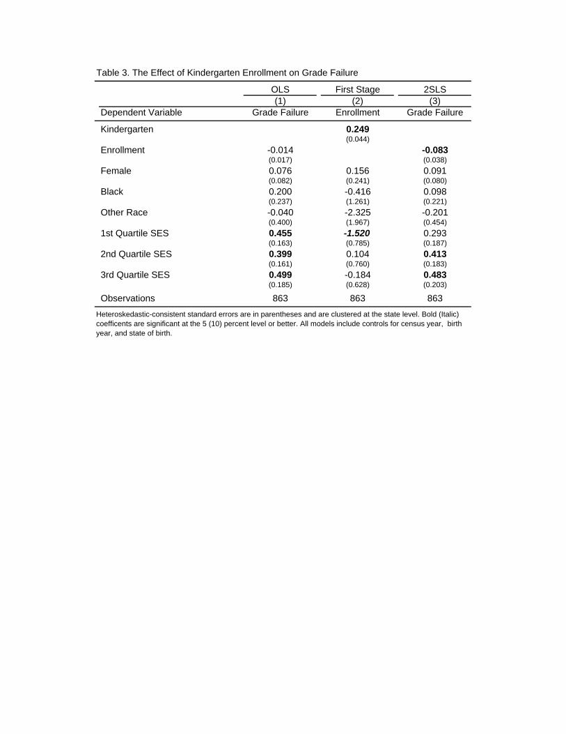
Table 3. The Effect of Kindergarten Enrollment on Grade Failure

OLS First Stage 2SLS(1) (2) (3)

Dependent Variable Grade Failure Enrollment Grade Failure

Kindergarten 0.249(0.044)

Enrollment -0.014 -0.083(0.017) (0.038)

Female 0.076 0.156 0.091(0.082) (0.241) (0.080)

Black 0.200 -0.416 0.098(0.237) (1.261) (0.221)

Other Race -0.040 -2.325 -0.201(0.400) (1.967) (0.454)

1st Quartile SES 0.455 -1.520 0.293(0.163) (0.785) (0.187)

2nd Quartile SES 0.399 0.104 0.413(0.161) (0.760) (0.183)

3rd Quartile SES 0.499 -0.184 0.483(0.185) (0.628) (0.203)

Observations 863 863 863Heteroskedastic-consistent standard errors are in parentheses and are clustered at the state level. Bold (Italic) coefficents are significant at the 5 (10) percent level or better. All models include controls for census year, birth year, and state of birth.

Female Male(1) (2)

Kindergarten (K) -0.021 -0.026(0.008) (0.010)

Black 0.021 0.018(0.006) (0.006)

Other Race 0.039 0.019(0.018) (0.019)

1st Quartile SES 0.115 0.139(0.009) (0.009)

2nd Quartile SES 0.049 0.067(0.003) (0.005)

3rd Quartile SES 0.021 0.029(0.001) (0.002)

Observations 1319135 1370607

Table 4. The Effect of State Subsidized Kindergarten on Grade Failure

Heteroskedastic-consistent standard errors are in parentheses and are clustered at the state level. Bold (Italic) coefficents are significant at the 5 (10) percent level or better. All models include fixed effects for age, birth year, and state of birth.

Female Male(1) (2)

Kindergarten (K) -0.016 -0.020(0.007) (0.010)

Kindergarten * Black -0.029 -0.037(0.011) (0.010)

Black 0.037 0.039(0.011) (0.010)

1st Quartile SES 0.114 0.137(0.009) (0.009)

2nd Quartile SES 0.049 0.067(0.003) (0.005)

3rd Quartile SES 0.021 0.029(0.001) (0.002)


White 5.0 4.1Black 6.1 7.8


F statistic for Joint Test of Kindergarten Effectiveness

Difference between Blacks and WhitesTable 5. The Effect of State Subsidized Kindergarten on Grade Failure

Female Male(1) (2)

Kindergarten (K) 0.003 -0.001(0.007) (0.010)

Kindergarten * 1st Quartile SES -0.062 -0.064(0.013) (0.013)

Kindergarten * 2nd Quartile SES -0.018 -0.020(0.007) (0.008)

Kindergarten * 3rd Quartile SES -0.005 -0.004(0.003) (0.004)

Black 0.018 0.015(0.006) (0.006)

Other Race 0.037 0.018(0.018) (0.019)

1st Quartile SES 0.154 0.179(0.012) (0.012)

2nd Quartile SES 0.062 0.082(0.006) (0.007)

3rd Quartile SES 0.026 0.033(0.003) (0.003)


F statistic for Joint Test of Kindergarten Effectiveness1st Quartile SES 12.8 12.72nd Quartile SES 3.7 3.63rd Quartile SES 1.5 0.64th Quartile SES 0.2 0.0

Heteroskedastic-consistent standard errors are in parentheses and are clustered at the statelevel. Bold (Italic) coefficents are significant at the 5 (10) percent level or better. All models include fixed effects for age, birth year, and state of birth.

Table 6. The Effect of State Subsidized Kindergarten on Grade FailureDifference between SES Quartiles

Female Male(1) (2)

Kindergarten -0.014 -0.021(0.011) (0.012)

Kindergarten * Relative Age Quarter 1 -0.003 0.026(0.012) (0.014)

Kindergarten * Relative Age Quarter 2 -0.012 -0.010(0.007) (0.007)

Kindergarten * Relative Age Quarter 3 -0.009 -0.004(0.006) (0.005)

Black 0.036 0.036(0.008) (0.010)

Other Race 0.112 0.101(0.021) (0.022)

1st Quartile SES 0.168 0.190(0.009) (0.010)

2nd Quartile SES 0.075 0.093(0.008) (0.007)

3rd Quartile SES 0.031 0.037(0.004) (0.005)

Relative Age Quarter 1 0.146 0.199(0.006) (0.007)




Q1 2.2 1.8Q2 2.9 4.0Q3 6.6 1.7Q4 1.8 3.1

Table 7. The Effect of State Subsidized Kindergarten on Grade FailureDifference between Relative Age Quarters



OLS First Stage 2SLS(1) (2) (3)

Panel A: Academic 9th Grade 0.004 0.306 0.008

(0.002) (0.049) (0.004)10th Grade 0.005 0.306 0.009

(0.003) (0.049) (0.005)11th Grade 0.006 0.306 0.010

(0.004) (0.049) (0.007)High School Graduate 0.009 0.306 0.013

(0.006) (0.049) (0.010)Some College -0.005 0.306 -0.027

(0.017) (0.049) (0.028)B.A. Degree -0.016 0.306 -0.028

(0.012) (0.049) (0.019)Advanced Degree 0.002 0.306 0.002

(0.002) (0.049) (0.005)

Panel B: Labor Market Usual Hours Worked -0.296 0.306 0.673

(0.236) (0.049) (0.483)Weeks Works -0.193 0.306 0.569

(0.232) (0.049) (0.456)Employed -0.007 0.306 0.010

(0.004) (0.049) (0.009)Yearly Income 375 0.306 1225

(401) (0.049) (827)Ln Yearly Income -0.002 0.306 0.001

(0.018) (0.049) (0.031)Ln Hourly Wages 0.009 0.306 -0.001

(0.011) (0.049) (0.020)

Table 8. The Effect of Enrollment in Kindergarten on Long Run Outcomes

Heteroskedastic-consistent standard errors are in parentheses and are clustered at the state level. Bold (Italic) coefficents are significant at the 5 (10) percent level or better. All models include controls for census year, birth year, and state of birth. There are 1115 observations in each regression.

Female Male(1) (2)

Panel A: Academic 9th Grade 0.004 0.006

(0.001) (0.002)10th Grade 0.005 0.006

(0.002) (0.002)11th Grade 0.007 0.008

(0.002) (0.003)High School Graduate 0.010 0.008

(0.003) (0.004)Some College -0.002 0.000

(0.008) (0.007)B.A. Degree -0.011 -0.003

(0.005) (0.005)Advanced Degree 0.002 0.010

(0.002) (0.003)

Panel B: Labor Market Employed 0.000 0.006

(0.004) (0.003)Usual Hours Worked -0.394 -0.038

(0.158) (0.080)Weeks Works -0.151 0.036

(0.061) (0.029)Yearly Income -365 320

(203) (207)Ln Hourly Wages -0.007 -0.001

(0.005) (0.004)

Table 9. The Effect of Enrollment in Kindergarten on Long Run Outcomes

Heteroskedastic-consistent standard errors are in parentheses and are clustered at the state level. Bold (Italic) coefficents are significant at the 5 (10) percent level or better. All models include fixed effects for birth year and state of birth. There are 1115 observations in each regression.

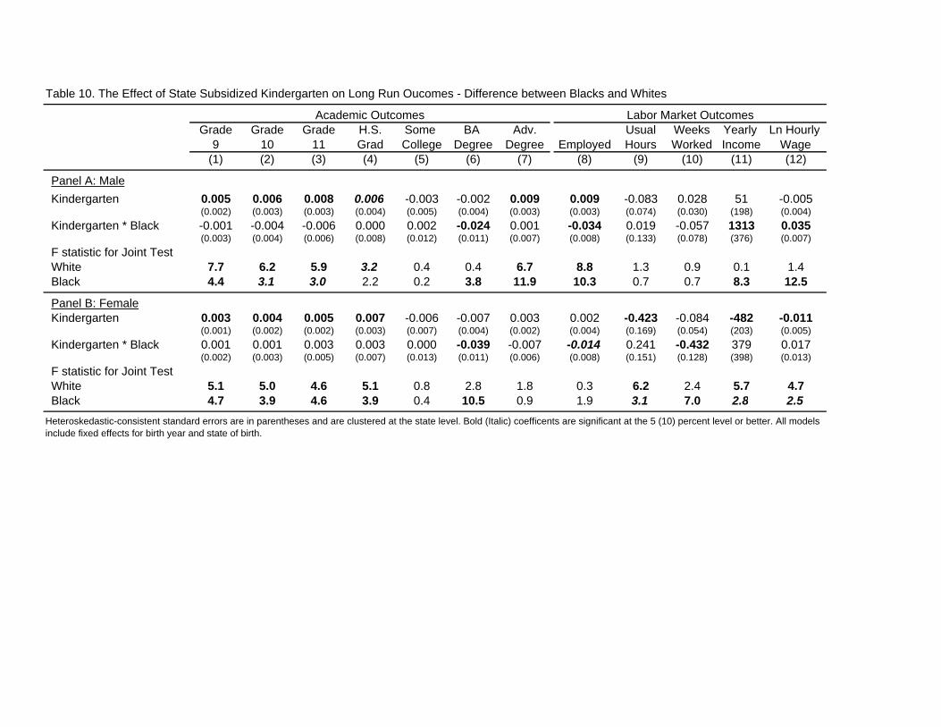
Table 10. The Effect of State Subsidized Kindergarten on Long Run Oucomes - Difference between Blacks and Whites

Grade Grade Grade H.S. Some BA Adv. Usual Weeks Yearly Ln Hourly 9 10 11 Grad College Degree Degree Employed Hours Worked Income Wage

(1) (2) (3) (4) (5) (6) (7) (8) (9) (10) (11) (12)

Panel A: MaleKindergarten 0.005 0.006 0.008 0.006 -0.003 -0.002 0.009 0.009 -0.083 0.028 51 -0.005

(0.002) (0.003) (0.003) (0.004) (0.005) (0.004) (0.003) (0.003) (0.074) (0.030) (198) (0.004)Kindergarten * Black -0.001 -0.004 -0.006 0.000 0.002 -0.024 0.001 -0.034 0.019 -0.057 1313 0.035

(0.003) (0.004) (0.006) (0.008) (0.012) (0.011) (0.007) (0.008) (0.133) (0.078) (376) (0.007)F statistic for Joint Test White 7.7 6.2 5.9 3.2 0.4 0.4 6.7 8.8 1.3 0.9 0.1 1.4Black 4.4 3.1 3.0 2.2 0.2 3.8 11.9 10.3 0.7 0.7 8.3 12.5

Panel B: FemaleKindergarten 0.003 0.004 0.005 0.007 -0.006 -0.007 0.003 0.002 -0.423 -0.084 -482 -0.011

(0.001) (0.002) (0.002) (0.003) (0.007) (0.004) (0.002) (0.004) (0.169) (0.054) (203) (0.005)Kindergarten * Black 0.001 0.001 0.003 0.003 0.000 -0.039 -0.007 -0.014 0.241 -0.432 379 0.017

(0.002) (0.003) (0.005) (0.007) (0.013) (0.011) (0.006) (0.008) (0.151) (0.128) (398) (0.013)F statistic for Joint TestWhite 5.1 5.0 4.6 5.1 0.8 2.8 1.8 0.3 6.2 2.4 5.7 4.7Black 4.7 3.9 4.6 3.9 0.4 10.5 0.9 1.9 3.1 7.0 2.8 2.5

Academic Outcomes

Heteroskedastic-consistent standard errors are in parentheses and are clustered at the state level. Bold (Italic) coefficents are significant at the 5 (10) percent level or better. All models include fixed effects for birth year and state of birth.

Labor Market Outcomes

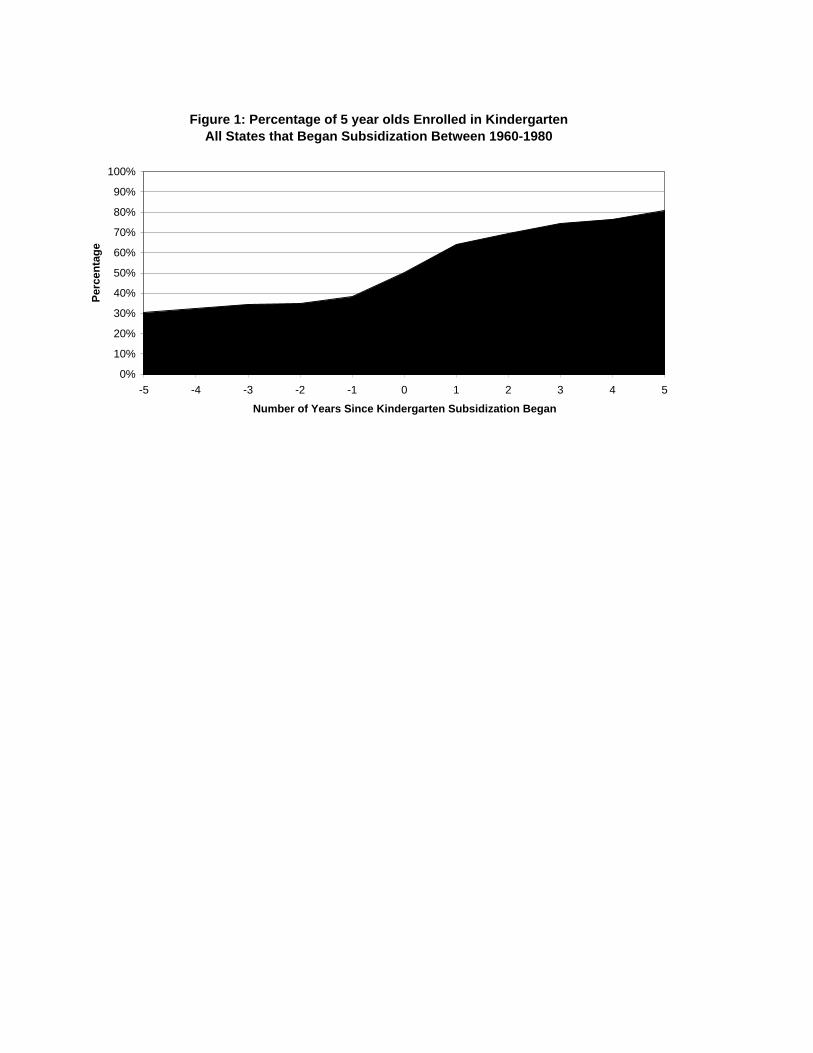
Figure 1: Percentage of 5 year olds Enrolled in Kindergarten All States that Began Subsidization Between 1960-1980

0%

10%

20%

30%

40%

50%

60%

70%

80%

90%

100%

-5 -4 -3 -2 -1 0 1 2 3 4 5

Number of Years Since Kindergarten Subsidization Began

Perc

enta

ge

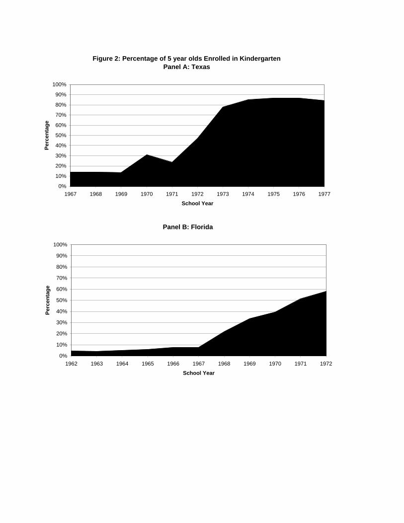
Figure 2: Percentage of 5 year olds Enrolled in Kindergarten Panel A: Texas

0%

10%

20%

30%

40%

50%

60%

70%

80%

90%

100%

1967 1968 1969 1970 1971 1972 1973 1974 1975 1976 1977

School Year

Perc

enta

ge

Panel B: Florida

0%

10%

20%

30%

40%

50%

60%

70%

80%

90%

100%

1962 1963 1964 1965 1966 1967 1968 1969 1970 1971 1972

School Year

Perc

enta

ge

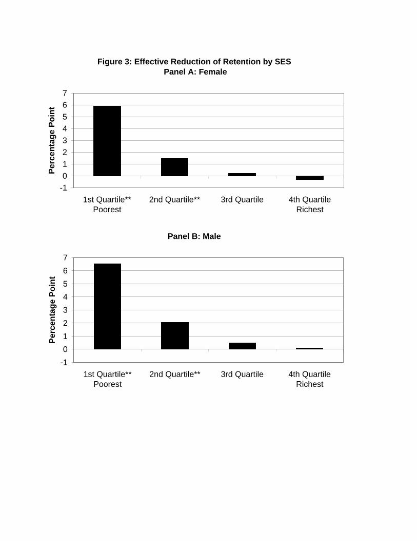
Figure 3: Effective Reduction of Retention by SES Panel A: Female

-101234567

1st Quartile**Poorest

2nd Quartile** 3rd Quartile 4th QuartileRichest

Perc

enta

ge P

oint

Panel B: Male

-101234567

1st Quartile**Poorest

2nd Quartile** 3rd Quartile 4th QuartileRichest

Perc

enta

ge P

oint

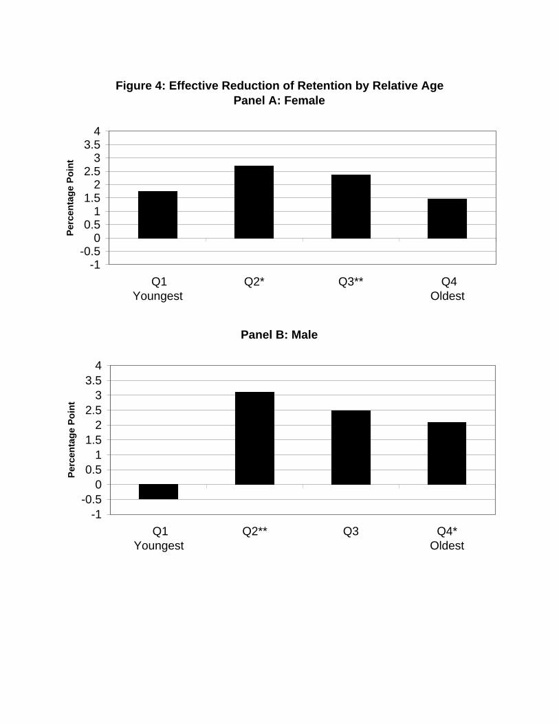
Figure 4: Effective Reduction of Retention by Relative Age Panel A: Female

-1-0.5

00.5

11.5

22.5

33.5

4

Q1 Youngest

Q2* Q3** Q4 Oldest

Perc

enta

ge P

oint

Panel B: Male

-1-0.5

00.5

11.5

22.5

33.5

4

Q1 Youngest

Q2** Q3 Q4* Oldest

Perc

enta

ge P

oint

(1) (2) (3) (4)

Kindergarten 0.001 0.281 0.055 0.246(0.041) (0.061) (0.057) (0.058)

Kindergarten * Relative Quarter 1 0.152 -0.451 0.128 -0.428(0.030) (0.050) (0.020) (0.041)

Kindergarten * Relative Quarter 2 0.158 -0.065 0.118 -0.040(0.035) (0.052) (0.026) (0.029)

Kindergarten * Relative Quarter 3 0.157 -0.065 0.158 0.020(0.025) (0.027) (0.019) (0.033)

Black 0.038 0.052 0.062 0.057(0.013) (0.023) (0.013) (0.018)

Other Race 0.013 0.092 0.048 0.011(0.027) (0.052) (0.019) (0.036)

1st Quartile SES -0.226 -0.169 -0.228 -0.177(0.036) (0.023) (0.046) (0.033)

2nd Quartile SES -0.136 -0.110 -0.136 -0.111(0.036) (0.025) (0.053) (0.030)

3rd Quartile SES -0.049 -0.056 -0.047 -0.051(0.015) (0.023) (0.031) (0.026)

Relative Quarter 1 (Youngest) -0.241 0.580 -0.204 0.550(0.029) (0.047) (0.011) (0.034)

Relative Quarter 2 -0.220 0.032 -0.177 -0.010(0.029) (0.035) (0.017) (0.022)

Relative Quarter 3 -0.214 0.015 -0.173 -0.043(0.022) (0.014) (0.011) (0.029)

Statewide Cutoff Date October 1 January 1 October 1 January 1

Observations 17100 10464 17898 11106

Q1 44.8 76.6 38.1 91.8Q2 12.9 11.5 17.4 12.9Q3 55.7 15.5 38.6 9.1Q4 0.0 21.5 0.9 18.2

Appendix Table 1. The Effect of State Subsidized Kindergarten on Enrollment of Five Year OldsDifference between Relative Quarters



Female Male

Appendix Table: Effect of Kindergarten on Enrollment of 5 yr olds

Panel A: Female, October 1 Cutoff

0

5

10

15

20

25

30

35

Q1** Q2** Q3** Q4

Perc

enta

ge P

oint

Panel B: Female, January 1 Cutoff

-20-15-10-505

101520253035

Q1** Q2** Q3** Q4**

Perc

enta

ge P

oint

Panel C: Male October 1 Cutoff

0

5

10

15

20

25

30

35

Q1** Q2** Q3** Q4

Perc

enta

ge P

oint

Panel D: Male, January 1 Cutoff

-20-15-10-505

101520253035

Q1** Q2** Q3** Q4**

Perc

enta

ge P

oint

Documents

Who Benefits from Kindergarten? Evidence from the ... · Who Benefits from Kindergarten? Evidence from the Introduction of State ... system occurred in all 50 ... representing enrollment