Embed Size (px)
DESCRIPTION
Wheres Cape Red User Guide
Citation preview
6.5.4
WhereScape RED User Guide
The software described in this book is furnished under a license agreement and may be used only in
accordance with the terms of the agreement.
WhereScape RED Tutorials
The software described in this book is furnished under a license agreement and may be used only in
accordance with the terms of agreement.
Copyright Notice
Copyright © 2002-2010 WhereScape Software Limited. All rights reserved. This document may be
redistributed in its entirety and in this electronic or printed form only without permission; all other uses of
this document and the information it contains require the explicit written permission of WhereScape
Software limited.
Due to continued product development this information may change without notice. WhereScape Software
Limited does not warrant that this document is error-free.
Trademarks
WhereScape and WhereScape RED are trademarks or registered trademarks of WhereScape Software
Limited. Other brands or product names are trademarks or registered trademarks of their respective
companies.
US Headquarters
2100 NW 133rd Place
Suite 76
Portland, OR 97229
United States
T: 503-466-3979
F: 503-466-3978
Asia/ Pacific Headquarters
Level 4, Wyndham Towers
38 Wyndham Street
Auckland
T: +64-9-358-5678
T: US toll free 1-877-237-3980
F: +64-9-358-5679
P.O.Box 56569
Auckland
New Zealand
European Headquarters
Albury House
14 Shute End
Wokingham
Berks RG40 1BJ
T: +44-118-914-4509
F: +44-118-914-4508
Contents i
Contents
1. Overview 1
2. Design Introduction 7
3. Objects and Windows 9
3.1 Object Types 9 3.2 Working with Objects 13 3.3 Organizing Objects 29
3.3.1 Adding Objects to Projects 32 3.3.2 Removing Objects from Projects 33 3.3.3 Using the Project/Object Maintenance Facility 34 3.3.4 Adding Projects to Groups 34 3.3.5 Removing Projects from Groups 35 3.3.6 Moving Projects within Groups 35
3.4 Windows and Panes 35 3.4.1 Browser window 36 3.4.1 Main Browser Window 39 3.4.2 Scheduler window 41 3.4.3 Diagrammatical window 42 3.4.4 Procedure Editor window 43
3.5 Database Error Messages 44
4. Tutorials 45
5. Settings and Parameters 47
5.1 Default Settings 47 5.1.1 Settings - Repository Attributes and Options 48 5.1.2 Settings - Objects Options 52 5.1.3 Settings - Table, Index and Key Name Defaults 57 5.1.4 Settings - Procedure Naming Defaults 59 5.1.5 Settings - Tablespace (Filegroup) Defaults 60 5.1.6 Settings - Ancillary Table and Column Defaults 61 5.1.7 Settings - Icons 65 5.1.8 Settings - Documentation 66 5.1.9 Settings - Statistics 68 5.1.10 Settings - Languages 71
5.2 Parameters 72
6. Connections 75
6.1 Connections Overview 75
ii Contents
6.2 Connection to the Data Warehouse 78 6.3 Connections to Another Database 84
6.3.1 Database Link Creation 91 6.4 ODBC Based Connections 93 6.5 Connections to Unix 95 6.6 Connections to Windows 99 6.7 Connections to Analysis Services 103
7. Table Properties 105
7.1 Table Storage Properties 106 7.1.1 Table Storage Screen - SQL Server 108 7.1.2 Table Storage Screen - Oracle 109 7.1.3 Table Storage Screen - DB2 111
7.2 Table Notes 111 7.2.1 Table Notes Screen 112
7.3 Table Documentation Fields 113 7.3.1 Table Documentation Fields Screen 114
7.4 Table Statistics in DB2 114 7.4.1 Table Statistics Screen 115
8. Loading Data 117
8.1 Choosing the Best Load Method 118 8.2 Load Drag and Drop 119
8.2.1 Data Type Mappings 119 8.3 Database Link Load 122
8.3.1 Database Link Load - Properties 122 8.3.2 Database Link Load - Source Mapping 125 8.3.3 Remote View Extract 129
8.4 ODBC Based Load 132 8.5 SSIS Loader 132
8.5.1 How to use SSIS loading in RED 133 8.5.2 Troubleshooting 136
8.6 Native ODBC Based Load 136 8.6.1 Native ODBC Based Load - Source Mapping 138 8.6.2 File Actions 142
8.7 Flat File Loads 145 8.7.1 File Load 149 8.7.2 Host Script Loads 152 8.7.3 File Wild Card Loads 152
8.8 XML File load 153 8.9 External Load 156 8.10 Handling Missing Source Columns 157 8.11 Load Table Transformations 159
8.11.1 Post-Load Procedures 159 8.12 Changing Load Connection and Schema 159
9. Dimensions 161
9.1 Dimensions Overview 162
Contents iii
9.2 Building a Dimension 164 9.3 Generating the Dimension Update Procedure 171 9.4 Dimension Artificial Keys 179 9.5 Dimension Get Key Function 180 9.6 Dimension Initial Build 181 9.7 Dimension Column Properties 182 9.8 Dimension Column Transformations 189 9.9 Dimension Hierarchies 189
9.9.1 Adding a Dimension Hierarchy 190 9.9.2 Using a Maintained Hierarchy 191
9.10 Snowflake 191 9.10.1 Creating a Snowflake 191
9.11 Dimension Language Mapping 193
10. Staging 195
10.1 Building the Stage Table 196 10.2 Generating the Staging Update Procedure 199 10.3 Tuning the Staging Update Process 210 10.4 Stage Table Column Properties 211 10.5 Stage Table Column Transformations 216
11. Data Store Objects 217
11.1 Data Store Object Overview 218 11.2 Building a Data Store Object 220 11.3 Generating the Data Store Update Procedure 224 11.4 Data Store Artificial Keys 235 11.5 Data Store Column Properties 237 11.6 Data Store Object Column Transformations 240
12. Normalized Tables 241
12.1 Normalized Tables Overview 242 12.2 Building a Normalized Table 244 12.3 Generating the Normalized Update Procedure 248 12.4 Normalized Table Artificial Keys 260 12.5 Normalized Table Column Properties 263 12.6 Normalized Table Column Transformations 267
13. Fact Tables 269
13.1 Detail Fact Tables 270 13.1.1 Creating Detail Fact Tables 270
13.2 Rollup or Combined Fact Tables 271 13.2.1 Creating Rollup Fact Tables 272
13.3 KPI Fact Tables 273 13.3.1 Creating the KPI Dimension 273 13.3.2 Creating KPI Fact Tables 274 13.3.3 Setup of KPI Fact Tables 275
iv Contents
13.4 Snapshot Fact Tables 281 13.4.1 Creating Snapshot Fact Tables 281
13.5 Slowly Changing Fact Tables 281 13.5.1 Creating Slowly Changing Fact Tables 282
13.6 Partitioned Fact Tables 282 13.6.1 Creating a Partitioned Fact Table in SQL Server 283 13.6.2 Creating a Partitioned Fact Table in Oracle 287 13.6.3 Creating a Partitioned Fact Table in DB2 291
13.7 Fact Table Column Properties 295 13.8 Fact Table Language Mapping 299
14. Aggregation 301
14.1 Creating an Aggregate Table 301 14.1.1 Change an Aggregates Default Look Back Days 304
14.2 Creating an Aggregate Summary Table 304
15. Views 307
15.1 Creating a Dimension View 308 15.1.1 View Column Re-mapping 312
15.2 Non-Dimension Object Views 313 15.3 Creating a Custom View 316 15.4 Dimension View Language Mapping 318
16. Analysis Services OLAP Cubes 319
16.1 Overview 319 16.2 Defining an OLAP Cube 320 16.3 Inspecting and Modifying Advanced Cube Properties 323 16.4 Creating an OLAP Cube on the Analysis Services Server 325 16.5 Cube Objects 326
16.5.1 Properties 326 16.5.2 Measure Groups 330 16.5.3 Measure Group Processing / Partitions 332 16.5.4 Measure Group Partitions 335 16.5.5 Measures 338 16.5.6 Calculations 341 16.5.7 Key Performance Indicators 344 16.5.8 Actions 347 16.5.9 Cube Dimensions 351 16.5.10 Measure Group Dimensions 353
16.6 Dimension Objects 356 16.6.1 Dimension Overview 356 16.6.2 Dimension Attributes 359 16.6.3 Attribute Relationships 362 16.6.4 Dimension Hierarchies 364 16.6.5 Dimension User Defined Hierarchy Levels 366
16.7 Changing OLAP Cubes 368 16.8 Retrofitting an OLAP Object 370
Contents v
17. Exporting Data 375
17.1 Building an Export Object 375 17.2 File Attributes 378
17.2.1 Export Object File Attributes Screen 380 17.3 Export Column Attributes 381
17.3.1 Export Column Attributes Screen 382 17.4 Host Script Exports 383
18. MicroStrategy Projects 385
18.1 MicroStrategy Prerequisites 385 18.2 Building MicroStrategy Projects 385
19. Transformations 387
19.1 Column Transformations 387 19.1.1 Column Transformation Properties 388 19.1.2 Load Table Column Transformations 390
19.2 Database Functions 393 19.3 Re-usable Transformations 393
19.3.1 Creating a New Re-usable Transformation 394 19.3.2 Changing a Re-usable Transformation 398 19.3.3 Using Re-usable Transformations 400
20. Procedures and Scripts 401
20.1 Procedure Generation 402 20.2 Procedure Editing 405 20.3 Procedure Loading and Saving 408 20.4 Procedure Comparisons 409 20.5 Procedure Compilation 410 20.6 Procedure Running 410 20.7 Procedure Syntax 411 20.8 Procedure Properties 412 20.9 Script Generation 413
20.9.1 Script Generation (Windows/SQL Server) 413 20.9.2 Script Generation (Unix/Oracle) 417 20.9.3 Script Generation (Windows/Oracle) 421 20.9.4 Script Generation (Windows/DB2) 424
20.10 Script Editing 427 20.11 Script Testing 428 20.12 Script Syntax 428 20.13 Templates 430
21. Scheduler 431
21.1 Scheduler Options 432 21.2 Scheduler States 435
vi Contents
21.3 Scheduling a Job 437 21.4 Editing Jobs 445 21.5 Deleting Job Logs 446 21.6 Monitoring the Database and Jobs 447
21.6.1 Database Monitoring 447 21.6.2 Job Monitoring 449
21.7 Stand Alone Scheduler Maintenance 454
22. Indexes 457
22.1 Index Definition 458 22.2 Index Storage Properties 464
22.2.1 Index Storage Screen - SQL Server 465 22.2.2 Index Storage Screen - Oracle 466 22.2.3 Index Storage Screen - DB2 467
22.3 Index Menu Options 468
23. Documentation and Diagrams 469
23.1 Creating Documentation 469 23.2 Batch Documentation Creation 472 23.3 Reading the Documentation 473 23.4 Diagrams 473
23.4.1 Star Schema diagram 476 23.4.2 Track Back diagram 477 23.4.3 Data Join Track Back diagram 480 23.4.4 Track Forward diagram 481 23.4.5 Linked Tables diagram 482 23.4.6 Job Dependencies diagram 483
23.5 Query Tool Access 485
24. Reports 487
24.1 Dimension-Fact Matrix 488 24.2 OLAP Dimension-Cube Matrix 489 24.3 Dimension Views of a Specified Dimension 490 24.4 Column Reports 491
24.4.1 Columns without Comments 492 24.4.2 All Column Transformations 494 24.4.3 Re-Usable Column Transformations 495 24.4.4 Column Track-Back 496
24.5 Table Reports 497 24.5.1 Tables without Comments 498 24.5.2 Load Tables by Connection 499 24.5.3 Records that failed a Dimension Join 500 24.5.4 External Source Table/files 502
24.6 Procedure Reports 502 24.6.1 Modified Procedures 503 24.6.2 Custom Procedures 504
24.7 Index Reports 504 24.7.1 Modified Indexes 505
Contents vii
24.8 Object Reports 506 24.8.1 Objects-Project Matrix 507 24.8.2 Modified Objects (excluding indexes) 509 24.8.3 Objects Checked-out 511 24.8.4 Loaded or Imported Objects 512
24.9 Job Reports 513 24.9.1 Object-Job Matrix 514 24.9.2 Jobs with an Object 516 24.9.3 Tasks of a Job 517 24.9.4 Object Performance History 518 24.9.5 Job Performance History 519 24.9.6 Task Performance History 520
25. Validate 521
25.1 Validate Meta-data 521 25.2 Validate Workflow Data 522 25.3 Validate Table Create Status 522 25.4 Validate Load Table Status 522 25.5 Validate Index Status 522 25.6 Validate Procedure Status 523 25.7 List Meta-data Tables not in the Database 523 25.8 List Database Tables not in the Meta-data 524 25.9 List Tables with no related Procedures or Scripts 525 25.10 List Procedures not related to a Table 526 25.11 Compare Meta-data Repository to another 527 25.12 Compare Meta-data Indexes to Database 530 25.13 List Duplicate Business Key Columns 531 25.14 Query Data Warehouse Objects 532
26. Promoting Between Environments 533
26.1 Applications 534 26.1.1 Application Creation 535 26.1.2 Application Loading 538
26.2 Importing Object Metadata 539 26.3 Importing Language Files 540 26.4 Data Warehouse Testing 542 26.5 Creating and Loading Applications from the Command Line 545
27. Backing Up and Restoring Metadata 547
27.1 Backup using DB Routines 548 27.2 Restoring DB Backups 551 27.3 Unloading Metadata 555 27.4 Loading an Unload 556
28. Altering Metadata 559
28.1 Validating Tables 560
viii Contents
28.2 Validating Source (Load) Tables 562 28.3 Validating Procedures 562 28.4 Altering Tables 563 28.5 Validating Indexes 564 28.6 Recompiling Procedures 564
29. Callable Procedures 565
29.1 Introduction to Callable Procedures 566 29.2 Terminology 567 29.3 Common Parameters 568 29.4 Ws_Api_Glossary 568 29.5 Ws_Connect_Replace 571 29.6 Ws_Job_Clear_Archive 576 29.7 Ws_Job_Clear_Logs 581 29.8 Ws_Job_Clear_Logs_By_Date 585 29.9 Ws_Job_Create 589 29.10 Ws_Job_CreateWait 595 29.11 Ws_Job_Dependency 601 29.12 Ws_Job_Release 607 29.13 Ws_Job_Restart 612 29.14 Ws_Job_Schedule 617 29.15 Ws_Job_Status 622 29.16 Ws_Load_Change 629 29.17 Ws_Maintain_Indexes 634 29.18 Ws_Sched_Status 638 29.19 Ws_Version_Clear 640 29.20 WsParameterRead 644 29.21 WsParameterReadG 647 29.22 WsParameterReadJ 650 29.23 WsParameterWrite 653 29.24 WsWrkAudit 656 29.25 WsWrkAuditBulk 659 29.26 WsWrkError 663 29.27 WsWrkErrorBulk 666 29.28 WsWrkTask 671
30. Retrofitting 675
30.1 Migrating the Data Warehouse Database Platform 675 30.2 Importing a Data Model 680 30.3 Re-Target Source Tables 684 30.4 Retro Copy Column Properties 686
30.4.1 Retro Copy Column Properties Screen 689
31. Integrating WhereScape RED into an Existing Warehouse 691
31.1 Rebuild 692 31.2 Integrate 692
31.2.1 Integrate, Host Scripts 693 31.2.2 Integrate, Selecting a Table Type 694
Contents ix
31.2.3 Integrate, Questions 695 31.2.4 Integrate, Procedures 698 31.2.5 Integrate, Views 699 31.2.6 Integrate, WhereScape Tables 699
Index 701

Chapter 1 1. Overview 1
Traditionally data warehouses take too long to build and are too hard to change. WhereScape RED is an
Integrated Development Environment to support the building and managing of data warehouses. It has the
flexibility to enable you to build a variety of architectures including:
enterprise data warehouses
dimensional data warehouses
data marts
user facing views, aggregates and summaries
In all cases the core values of WhereScape RED are twofold: its rapid building capabilities that enable
better data warehouses to be built, faster, and its integrated environment that simplifies management.
As a data warehouse specific tool, WhereScape RED embodies a simple, pragmatic approach to
building data warehouses. With WhereScape RED you specify what you want to achieve by dragging
and dropping objects to create a meta view, and then let WhereScape RED do the heavy lifting of
creating the necessary tables and procedures etc. Data warehouse wizards prompt for additional
information at critical points to provide the maximum value from the generated objects.
Different data warehousing approaches including agile,prototyping and waterfall are supported by
WhereScape RED. Agile developers will find specific functionality has been included to support common
agile practices. For developers who are new to data warehousing, or are looking for a fast, pragmatic
approach, WhereScape's Pragmatic Data Warehousing Methodology can be used.
The basic concepts behind WhereScape's Pragmatic Data Warehousing Methodology are:
minimize the impact on the source systems
centralize management within the data warehouse
store transactional data at the lowest practical grain within the data warehouse
snapshot, combine and rollup transactional tables to provide additional value
utilize star schemas, views or cubes for end user access
allow for incremental loads from day one
use an iterative approach
minimize cleansing and transformations to ease source system reconciliation
design the data warehouse independently from the end user tool layer
WhereScape RED supports these concepts to facilitate very rapid delivery of data warehouses.
Data Flow - dimensional models
WhereScape RED controls the flow of data from the source systems through transforming and modelling
layers to analysis areas. Different styles of data warehousing (normalized, dimensional etc) are supported
and utilize different objects, but all follow the same basic flow. While some of these stages can be skipped,
the expected flow for the common approaches are:
C H A P T E R 1
1. Overview
2 1. Overview
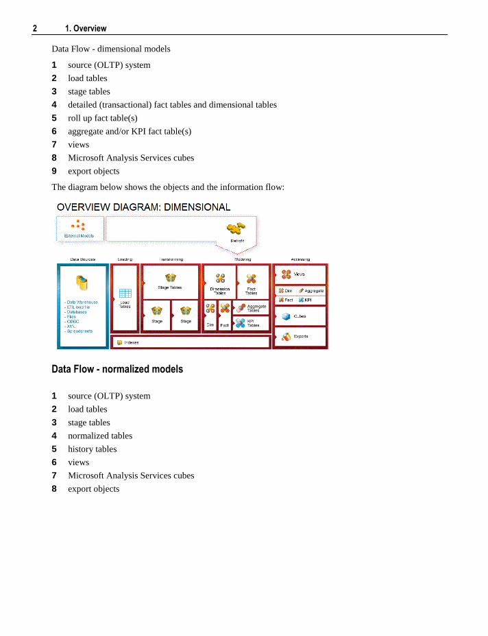
Data Flow - dimensional models
1 source (OLTP) system
2 load tables
3 stage tables
4 detailed (transactional) fact tables and dimensional tables
5 roll up fact table(s)
6 aggregate and/or KPI fact table(s)
7 views
8 Microsoft Analysis Services cubes
9 export objects
The diagram below shows the objects and the information flow:
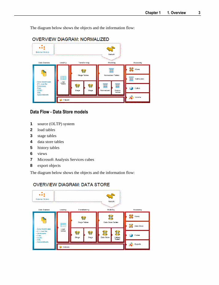
Data Flow - normalized models
1 source (OLTP) system
2 load tables
3 stage tables
4 normalized tables
5 history tables
6 views
7 Microsoft Analysis Services cubes
8 export objects
Chapter 1 1. Overview 3
The diagram below shows the objects and the information flow:
Data Flow - Data Store models
1 source (OLTP) system
2 load tables
3 stage tables
4 data store tables
5 history tables
6 views
7 Microsoft Analysis Services cubes
8 export objects
The diagram below shows the objects and the information flow:
4 1. Overview
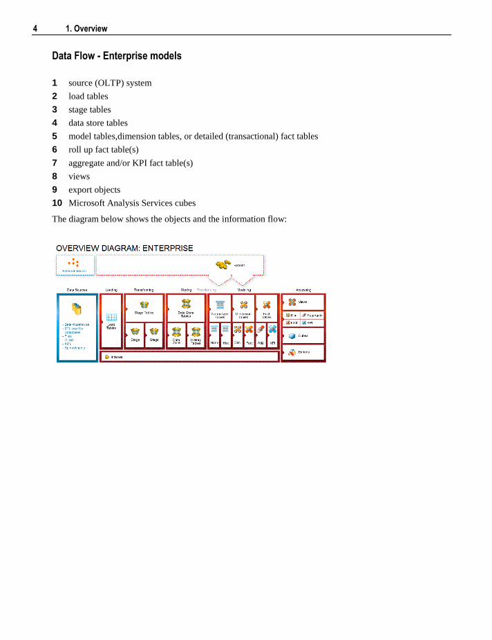
Data Flow - Enterprise models
1 source (OLTP) system
2 load tables
3 stage tables
4 data store tables
5 model tables,dimension tables, or detailed (transactional) fact tables
6 roll up fact table(s)
7 aggregate and/or KPI fact table(s)
8 views
9 export objects
10 Microsoft Analysis Services cubes
The diagram below shows the objects and the information flow:
Chapter 1 1. Overview 5
Data Flow
Data is moved from source tables to load tables via scripts, database links and ODBC links. These load
tables are created by dragging and dropping from a connection object. Load tables are generally based on
source system tables. Their main purpose is to be a destination for moving data as simply and quickly as
possible from the source system. Load tables will generally hold a single unit of data (e.g. last night or last
month), and will be truncated at the start of each extract. Transformations can be performed on the
columns during the load process if required.
Load tables feed stage tables, which in turn feed data store,model or dimension tables. Data from multiple
load tables can be combined at this level.
First tier transactional tables (fact or model) are created and updated from stage tables. Second tier tables
(model, summary rollup, aggregate, KPI etc) are created and updated from lower level tables.
Cubes can be created from transactional tables or views.
Procedural code
WhereScape RED generates procedural code in the target database's native language (e.g. PL/SQL for
Oracle) at each stage in the data warehouse build process. The generated code is, in nearly all cases,
sufficient to create a rapid prototype of the data warehouse.
While the generation of code is often seen as a key benefit of WhereScape RED, the ability to control and
manage custom code is also critical to the long term management of the data warehouse environment.
In most cases 85-100% of the generated code will be taken through to production with no customization
required.
Scheduler
The flow of data from the source systems to data warehouse tables is controlled and managed by the
WhereScape RED scheduler. All generated code includes audit and error logging logic that is used by the
scheduler.
The scheduler provides a single point of control for the warehouse. From the scheduler the state of all jobs
can be ascertained. Any warning or error messages can be investigated, and should a problem occur the
scheduler controls the restart of the job from the point of failure.
Documentation
Documenting the warehouse is often a task left until last, and in many cases done once (if at all!) and not
kept up to date. WhereScape RED generates user and technical documentation, including diagrams, in
HTML format.
Technical documentation includes copies of all current procedures.
User documentation includes a glossary of business terms available independently of any end user tool.
Where additional specific information needs to be included in the documentation, WhereScape RED
supports the inclusion of custom HTML pages in the generated output. This means in many cases the
entire documentation requirements can be managed from one location, and regenerated as changes occur.
6 1. Overview
WhereScapeRED and Traditional ETL Tools
WhereScape RED's core strength is in the rapid building of data warehouse structures. Organizations that
have already purchased traditional ETL tools can use WhereScape RED as a pureplay data warehouse
toolset. WhereScape RED can be used to iteratively build data marts or presentation layer objects that need
to be constantly updated to keep relevant for end users. In mosts cases customers will find that WhereScape
RED has enough ETL capabilities to build the entire data warehouse, using the database rather than a
proprietary engine to perform ETL processing.
The cross over in functionality between ETL tools and WhereScape RED is not large. WhereScape RED is
tightly integrated into the data warehouse database and has an embedded data warehouse building approach.
For WhereScape data movement is the start of the process - from source system to load tables. The key
benefits of the product: development productivity and an integrated environment to manage and maintain
your warehouse, come after the data movement stage. Where a traditional ETL tool is already in use, the
output of the ETL process is a WhereScape RED's Load, Stage, Dimension, Fact or Model table from which
WhereScape RED builds more advanced data warehouse structures.
Chapter 2 2. Design Introduction 7
Design Introduction
WhereScape RED can be used to build data warehouses based on any number of design philosophies from
normalized enterprise data warehouses with consumer data marts through to federated or conformed star
schema based warehouses. In the absence of another approach, the following methodology can be used for
the design of data warehouses.
Note: This section can be skipped if you already have data warehouse design experience or a methodology
you wish to utilize. It is meant to provide the novice designer with some tips for designing a data
warehouse.
Design Approach
The concepts behind the WhereScape Pragmatic Data Warehouse Methodology are as follows:
1 Building an enterprise-wide data warehouse is a process - an evolution rather than a big bang. Start
small and grow the warehouse in manageable chunks until all the pieces are in place. Once you reach
that stage, changes and new source systems will continue the process.
2 You need to understand the big picture, but not get lost in it. Talk to all the various departments,
business units and companies within the organization. Do so at a relatively high level and try to
understand how the information from each area impacts or affects the others. Identify commonalities
and areas where the same information is handled in different ways. This process should take days or
weeks not months.
3 Identify the high value, high return and possibly easiest areas of the business. Drill down in these
areas and break down the workload into small manageable chunks of work, for example, one to two
analysis areas. Agree on the first component of the data warehouse and do that.
4 Get an understanding of the source system for this first component or analysis area. If possible, get an
entity relationship diagram and talk to the people who built or support the application. Identify the
tables that contain the key information you will need. The goal is a quick and initial view, a detailed
specification is not required.
5 Design the first component. This design should be a first draft, and can be written rather than using a
design tool. Remember at this stage what the end users want is not really known, so don't set the
design in concrete, or spend a large amount of time in this area.
Note: Experienced users of WhereScape RED will often dispense with a design and go straight to
building a prototype.
6 Build a prototype. In most cases this should not take more than one or two weeks - experienced
WhereScape RED developers can expect to build prototypes in hours or days. Concentrate on the
detailed and descriptive data, unless you have a clear picture of the summarized requirements. Do as
much as possible in terms of validating the data back to the source system. If dealing with a large or
complex source system then only deliver a segment in this prototype, e.g, one branch, one store, one
product group, etc. Keep It Simple.
C H A P T E R 2
2. Design Introduction
8 2. Design Introduction
7 Demonstrate the prototype to a group of the key users. Then drill down to a subset of key users (we
recommend no more than three) who will help you go forward with the design. If possible give these
users access to the prototype and get them using the data. Stress that data accuracy is not the issue at
this stage, rather the look and feel.
8 Enhance the prototype with the feedback provided by the users. Again a quick process. If
complicated requirements evolve then create a plan to implement, doing the highest value parts first.
The goal is to get quick buy in and support from the two or three key users.
9 Provide key users access to the reworked prototype and get them using the data. Have them define the
business names for all the measures and attributes, and to define any pre-calculated measures that they
frequently use. Get them to define the hierarchies in the data. Ascertain the commonly utilized
queries and reports, and see if there would be a better way of presenting these.
10 From the user feedback look at the need or possibility of using higher level fact tables, such as
summaries, aggregates, snapshot or composite rollup tables.
The concepts and methodologies for designing and building a data warehouse are beyond the scope of this
manual. It is assumed that the reader understands the basic concepts of a data warehouse, and is familiar
with modelling, normalized, star and snowflake schemas, dimensions, fact tables, etc. Refer to the
WhereScape web site for a basic overview of data warehouse design if required.
Chapter 3 3. Objects and Windows 9
WhereScape RED makes use of an object concept when dealing with the different components that make up
a data warehouse solution. The main object types are: Connection, Load Table, Dimension, Stage Table,
Fact Table, Aggregate, Cube, Procedure, Host Script, Index, Export and Retro Copy.
This chapter explains and provides an overview of each of these object types and how they can be managed
and organized. The full functionality of each object is covered in the following chapters.
The various Windows, Panes and Views that form the WhereScape RED tool are also explained.
In This Chapter
3.1 Object Types ......................................................................... 9
3.2 Working with Objects ........................................................... 13
3.3 Organizing Objects ............................................................... 29
3.4 Windows and Panes .............................................................. 35
3.5 Database Error Messages ...................................................... 44
3.1 Object Types
WhereScape RED has a concept of objects which are combined to create real world data warehouses and
data marts, fast. Each WhereScape RED object has properties that allow the data warehouse developer to
change how the object is used.
Note: Some object types may not be available for certain types of WhereScape RED licenses.
WhereScape RED objects include:
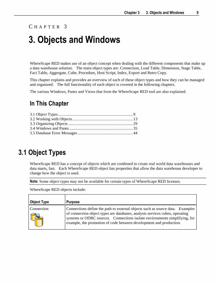
Object Type Purpose
Connection
Connections define the path to external objects such as source data. Examples
of connection object types are databases, analysis services cubes, operating
systems or ODBC sources. Connections isolate environments simplifying, for
example, the promotion of code between development and production.
C H A P T E R 3
3. Objects and Windows
10 3. Objects and Windows
Object Type Purpose
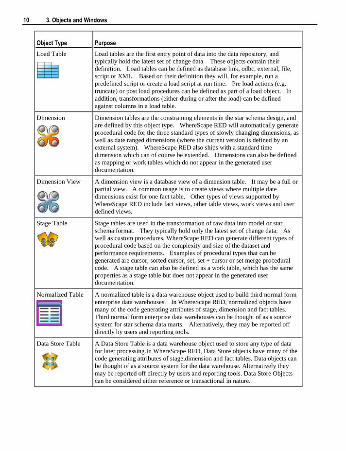
Load Table
Load tables are the first entry point of data into the data repository, and
typically hold the latest set of change data. These objects contain their
definition. Load tables can be defined as database link, odbc, external, file,
script or XML. Based on their definition they will, for example, run a
predefined script or create a load script at run time. Pre load actions (e.g.
truncate) or post load procedures can be defined as part of a load object. In
addition, transformations (either during or after the load) can be defined
against columns in a load table.
Dimension
Dimension tables are the constraining elements in the star schema design, and
are defined by this object type. WhereScape RED will automatically generate
procedural code for the three standard types of slowly changing dimensions, as
well as date ranged dimensions (where the current version is defined by an
external system). WhereScape RED also ships with a standard time
dimension which can of course be extended. Dimensions can also be defined
as mapping or work tables which do not appear in the generated user
documentation.
Dimension View
A dimension view is a database view of a dimension table. It may be a full or
partial view. A common usage is to create views where multiple date
dimensions exist for one fact table. Other types of views supported by
WhereScape RED include fact views, other table views, work views and user
defined views.
Stage Table
Stage tables are used in the transformation of raw data into model or star
schema format. They typically hold only the latest set of change data. As
well as custom procedures, WhereScape RED can generate different types of
procedural code based on the complexity and size of the dataset and
performance requirements. Examples of procedural types that can be
generated are cursor, sorted cursor, set, set + cursor or set merge procedural
code. A stage table can also be defined as a work table, which has the same
properties as a stage table but does not appear in the generated user
documentation.
Normalized Table
A normalized table is a data warehouse object used to build third normal form
enterprise data warehouses. In WhereScape RED, normalized objects have
many of the code generating attributes of stage, dimension and fact tables.
Third normal form enterprise data warehouses can be thought of as a source
system for star schema data marts. Alternatively, they may be reported off
directly by users and reporting tools.
Data Store Table
A Data Store Table is a data warehouse object used to store any type of data
for later processing.In WhereScape RED, Data Store objects have many of the
code generating attributes of stage,dimension and fact tables. Data objects can
be thought of as a source system for the data warehouse. Alternatively they
may be reported off directly by users and reporting tools. Data Store Objects
can be considered either reference or transactional in nature.
Chapter 3 3. Objects and Windows 11
Object Type Purpose
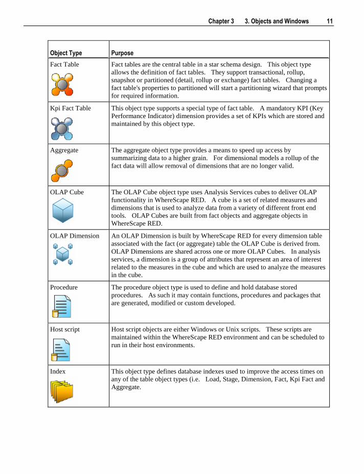
Fact Table
Fact tables are the central table in a star schema design. This object type
allows the definition of fact tables. They support transactional, rollup,
snapshot or partitioned (detail, rollup or exchange) fact tables. Changing a
fact table's properties to partitioned will start a partitioning wizard that prompts
for required information.
Kpi Fact Table
This object type supports a special type of fact table. A mandatory KPI (Key
Performance Indicator) dimension provides a set of KPIs which are stored and
maintained by this object type.
Aggregate
The aggregate object type provides a means to speed up access by
summarizing data to a higher grain. For dimensional models a rollup of the
fact data will allow removal of dimensions that are no longer valid.
OLAP Cube
The OLAP Cube object type uses Analysis Services cubes to deliver OLAP
functionality in WhereScape RED. A cube is a set of related measures and
dimensions that is used to analyze data from a variety of different front end
tools. OLAP Cubes are built from fact objects and aggregate objects in
WhereScape RED.
OLAP Dimension
An OLAP Dimension is built by WhereScape RED for every dimension table
associated with the fact (or aggregate) table the OLAP Cube is derived from.
OLAP Dimensions are shared across one or more OLAP Cubes. In analysis
services, a dimension is a group of attributes that represent an area of interest
related to the measures in the cube and which are used to analyze the measures
in the cube.
Procedure
The procedure object type is used to define and hold database stored
procedures. As such it may contain functions, procedures and packages that
are generated, modified or custom developed.
Host script
Host script objects are either Windows or Unix scripts. These scripts are
maintained within the WhereScape RED environment and can be scheduled to
run in their host environments.
Index
This object type defines database indexes used to improve the access times on
any of the table object types (i.e. Load, Stage, Dimension, Fact, Kpi Fact and
Aggregate.
12 3. Objects and Windows
Object Type Purpose
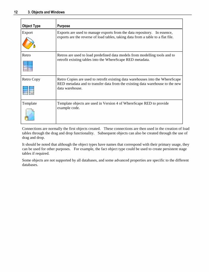
Export
Exports are used to manage exports from the data repository. In essence,
exports are the reverse of load tables, taking data from a table to a flat file.
Retro
Retros are used to load predefined data models from modelling tools and to
retrofit existing tables into the WhereScape RED metadata.
Retro Copy
Retro Copies are used to retrofit existing data warehouses into the WhereScape
RED metadata and to transfer data from the existing data warehouse to the new
data warehouse.
Template
Template objects are used in Version 4 of WhereScape RED to provide
example code.
Connections are normally the first objects created. These connections are then used in the creation of load
tables through the drag and drop functionality. Subsequent objects can also be created through the use of
drag and drop.
It should be noted that although the object types have names that correspond with their primary usage, they
can be used for other purposes. For example, the fact object type could be used to create persistent stage
tables if required.
Some objects are not supported by all databases, and some advanced properties are specific to the different
databases.
Chapter 3 3. Objects and Windows 13
3.2 Working with Objects
Most object types perform some form of action in the data warehouse. For example dimension, stage, fact
and aggregate table based objects are 'Updated' in the data warehouse via the defined update procedure.
Procedures can be executed in the database.
When positioned on an Object in the left hand pane of the WhereScape RED browser window, the right
mouse pop-up menu provides a number of options for manipulating the object. Further options may be
available through the menus provided in the various windows.
The operations of each of the objects is discussed in the following chapters. A brief overview of some of
the more common operations follows:
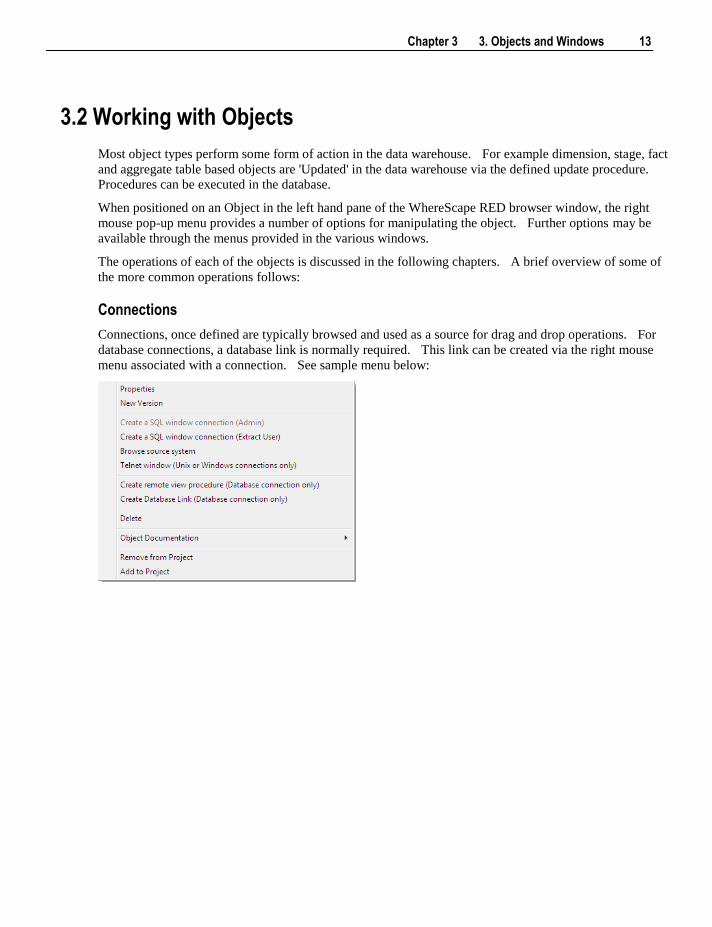
Connections
Connections, once defined are typically browsed and used as a source for drag and drop operations. For
database connections, a database link is normally required. This link can be created via the right mouse
menu associated with a connection. See sample menu below:
14 3. Objects and Windows
Other operations available through the menu are editing the properties of the connection, creating a version
of the connection, creating a telnet window for Unix connections and creating a remote view creation
procedure where required for database connections and loads.
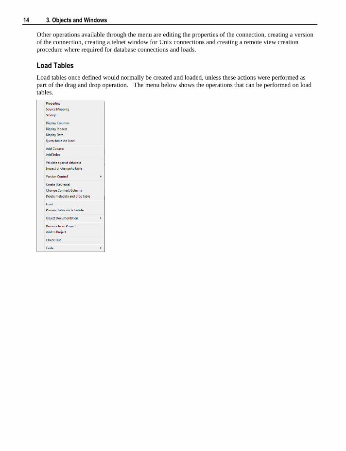
Load Tables
Load tables once defined would normally be created and loaded, unless these actions were performed as
part of the drag and drop operation. The menu below shows the operations that can be performed on load
tables.
Chapter 3 3. Objects and Windows 15
Properties, Source Mapping and Storage all launch the properties window for the load table, albeit focused
on different tabs within this window.
The columns and indexes of the load table can be displayed using Display Columns and Display Indexes.
Any data in the load table can be displayed using Display Data. If the data is displayed, only the first 100
rows are returned from the table. Either the Sql Admin tool (accessible via the WhereScape start menu
option), or the Excel query will have to be used if more detailed data analysis is required.
TIP: When a column list has been displayed in the central pane, it is sorted based on the 'order' field
associated with each column. A click on the column label 'Col name' will sort the columns into
alphabetical order. A subsequent click will re-sort based on the 'order' field.
New columns and indexes can be manually added through this menu using Add Column and Add Index.
Normally columns are added via drag and drop and most common indexes are created during the procedure
generation phase.
The metadata for the load table can be compared with the physical table resident in the database using
Validate against database, and where required the table altered to match the metadata. You can produce a
list of objects that will be potentially impacted by a change to the load table structure using Impact of change to table.
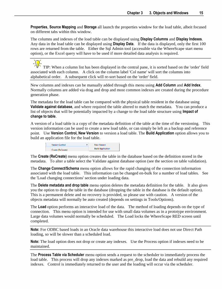
A version of a load table is a copy of the metadata definition of the table at the time of the versioning. This
version information can be used to create a new load table, or can simply be left as a backup and reference
point. Use Version Control, New Version to version a load table. The Build Application option allows you to
build an application file for the load table.
The Create (ReCreate) menu option creates the table in the database based on the definition stored in the
metadata. To alter a table select the Validate against database option (see the section on table validation).
The Change Connect/Schema menu option allows for the rapid changing of the connection information
associated with the load table. This information can be changed en-bulk for a number of load tables. See
the 'Load changing connections' section under loading data.
The Delete metadata and drop table menu option deletes the metadata definition for the table. It also gives
you the option to drop the table in the database (dropping the table in the database is the default option).
This is a permanent delete and no recovery is provided, so please use with caution. A version of the
objects metadata will normally be auto created (depends on settings in Tools/Options).
The Load option performs an interactive load of the data. The method of loading depends on the type of
connection. This menu option is intended for use with small data volumes as in a prototype environment.
Large data volumes would normally be scheduled. The Load locks the WhereScape RED screen until
completed.
Note: For ODBC based loads in an Oracle data warehouse this interactive load does not use Direct Path
loading, so will be slower than a scheduled load.
Note: The load option does not drop or create any indexes. Use the Process option if indexes need to be
maintained.
The Process Table via Scheduler menu option sends a request to the scheduler to immediately process the
load table. This process will drop any indexes marked as pre_drop, load the data and rebuild any required
indexes. Control is immediately returned to the user and the loading will occur via the scheduler.
16 3. Objects and Windows
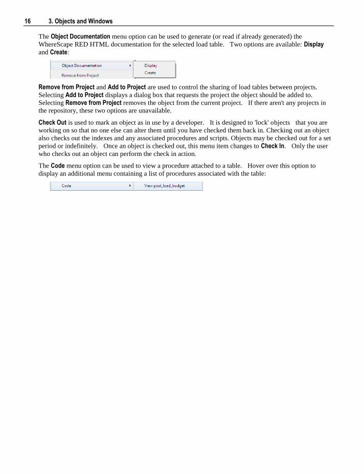
The Object Documentation menu option can be used to generate (or read if already generated) the
WhereScape RED HTML documentation for the selected load table. Two options are available: Display
and Create:
Remove from Project and Add to Project are used to control the sharing of load tables between projects.
Selecting Add to Project displays a dialog box that requests the project the object should be added to.
Selecting Remove from Project removes the object from the current project. If there aren't any projects in
the repository, these two options are unavailable.
Check Out is used to mark an object as in use by a developer. It is designed to 'lock' objects that you are
working on so that no one else can alter them until you have checked them back in. Checking out an object
also checks out the indexes and any associated procedures and scripts. Objects may be checked out for a set
period or indefinitely. Once an object is checked out, this menu item changes to Check In. Only the user
who checks out an object can perform the check in action.
The Code menu option can be used to view a procedure attached to a table. Hover over this option to
display an additional menu containing a list of procedures associated with the table:
Chapter 3 3. Objects and Windows 17
Choose a procedure from the list to open in the procedure editor in view mode.
Note: Only load tables with one or more defined procedures have the view code option.
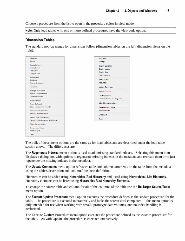
Dimension Tables
The standard pop-up menus for dimensions follow (dimension tables on the left, dimension views on the
right):
The bulk of these menu options are the same as for load tables and are described under the load table
section above. The differences are:
The Regenerate Indexes menu option is used to add missing standard indexes. Selecting this menu item
displays a dialog box with options to regenerate missing indexes in the metadata and recreate them or to just
regenerate the missing indexes in the metadata.
The Update Comments menu option refreshes table and column comments on the table from the metadata
using the table's description and columns' business definition.
Hierarchies can be added using Hierarchies /Add Hierarchy and listed using Hierarchies / List Hierarchy.
Hierarchy elements can be listed using Hierarchies /List Hierarchy Elements.
To change the source table and column for all of the columns of the table use the Re-Target Source Table
menu option.
The Execute Update Procedure menu option executes the procedure defined as the 'update procedure' for the
table. The procedure is executed interactively and locks the screen until completed. This menu option is
only intended for use when working with small / prototype data volumes, and no index handling is
performed.
The Execute Custom Procedure menu option executes the procedure defined as the 'custom procedure' for
the table. As with Update, the procedure is executed interactively.
18 3. Objects and Windows
The Execute Custom Procedure via Scheduler menu option executes the procedure defined as the 'custom
procedure' for the table, via the Scheduler.
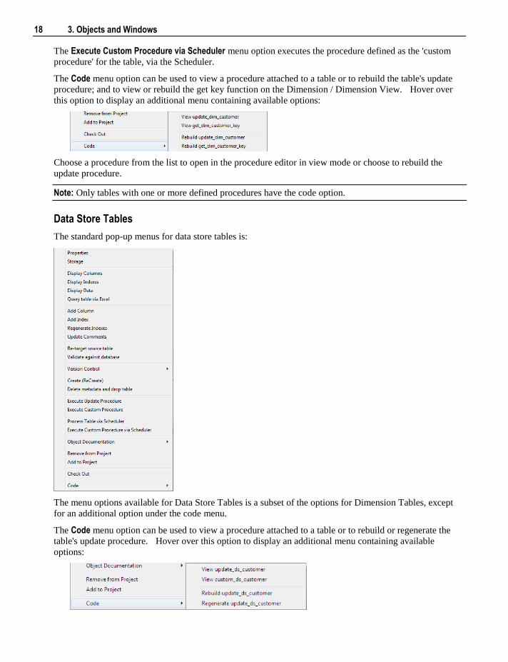
The Code menu option can be used to view a procedure attached to a table or to rebuild the table's update
procedure; and to view or rebuild the get key function on the Dimension / Dimension View. Hover over
this option to display an additional menu containing available options:
Choose a procedure from the list to open in the procedure editor in view mode or choose to rebuild the
update procedure.
Note: Only tables with one or more defined procedures have the code option.
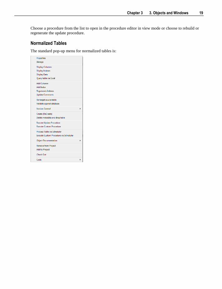
Data Store Tables
The standard pop-up menus for data store tables is:
The menu options available for Data Store Tables is a subset of the options for Dimension Tables, except
for an additional option under the code menu.
The Code menu option can be used to view a procedure attached to a table or to rebuild or regenerate the
table's update procedure. Hover over this option to display an additional menu containing available
options:
Chapter 3 3. Objects and Windows 19
Choose a procedure from the list to open in the procedure editor in view mode or choose to rebuild or
regenerate the update procedure.
Normalized Tables
The standard pop-up menu for normalized tables is:
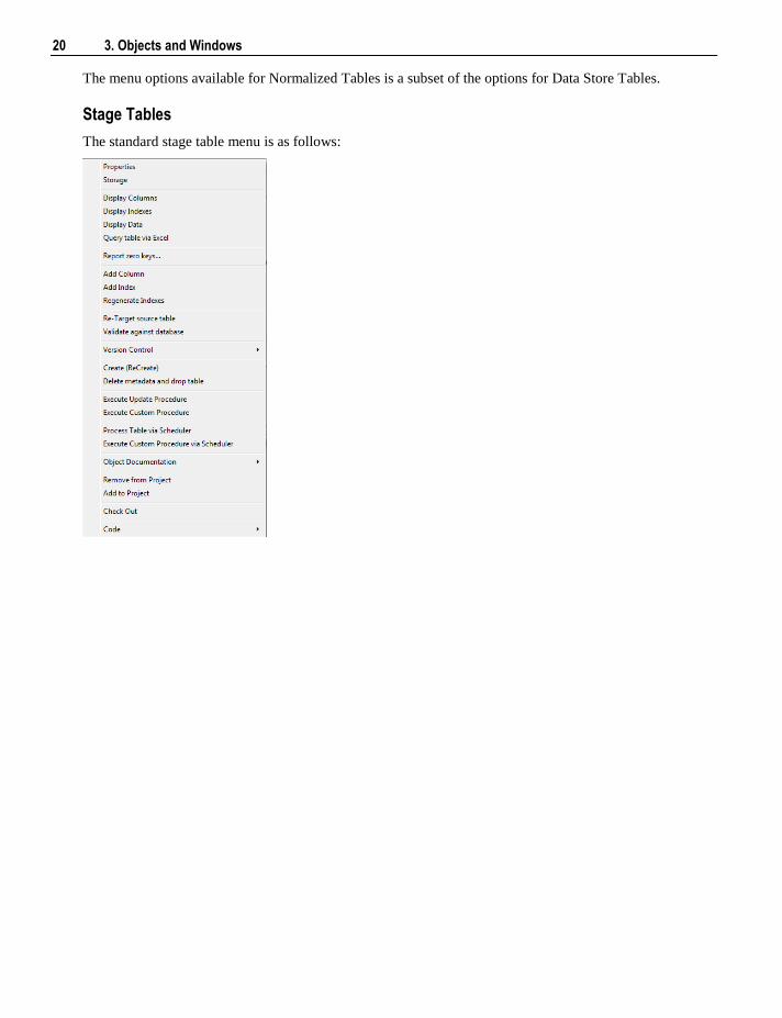
20 3. Objects and Windows
The menu options available for Normalized Tables is a subset of the options for Data Store Tables.
Stage Tables
The standard stage table menu is as follows:
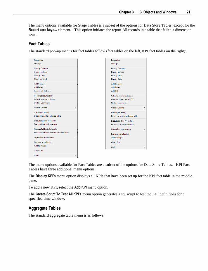
Chapter 3 3. Objects and Windows 21
The menu options available for Stage Tables is a subset of the options for Data Store Tables, except for the
Report zero keys... element. This option initiates the report All records in a table that failed a dimension
join...
Fact Tables
The standard pop-up menus for fact tables follow (fact tables on the left, KPI fact tables on the right):
The menu options available for Fact Tables are a subset of the options for Data Store Tables. KPI Fact
Tables have three additional menu options:
The Display KPI's menu option displays all KPIs that have been set up for the KPI fact table in the middle
pane.
To add a new KPI, select the Add KPI menu option.
The Create Script To Test All KPI's menu option generates a sql script to test the KPI definitions for a
specified time window.
Aggregate Tables
The standard aggregate table menu is as follows:
22 3. Objects and Windows
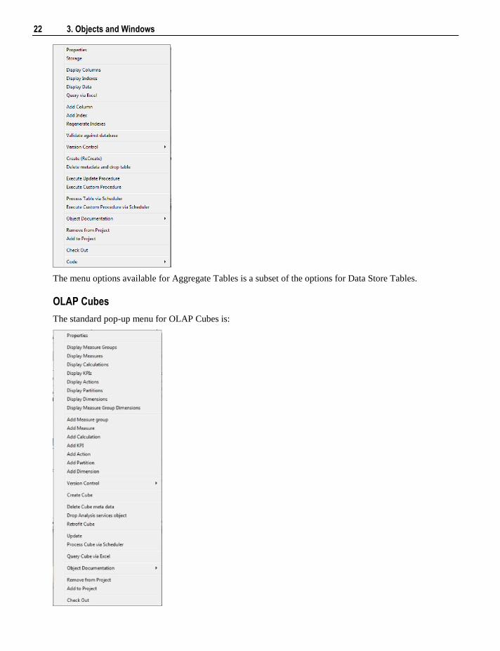
The menu options available for Aggregate Tables is a subset of the options for Data Store Tables.
OLAP Cubes
The standard pop-up menu for OLAP Cubes is:
Chapter 3 3. Objects and Windows 23
The Properties menu option opens the properties dialog that defines cube creation options and access to
documentation tabs.
The Display Measure Groups menu option shows the details of the measure groups associated with the cube
in the centre pane.
The Display Measures menu option lists the measures associated with the measure groups in the cube. This
is the default view in the middle pane when a cube is selected in the left pane with a single click.
The Display Calculations option lists all the calculated members defined in the cube.
The Display KPIs lists all the Key Performance Indicators defined in the cube.
The Display Actions option lists all the actions defined in the cube.
The Display Partitions option lists all the partitions defined against the related measure groups within the
cube.
The Display Dimensions option lists all of the dimensions defined in the cube.
The Display Measure Group Dimensions option displays a cross tab report in the centre pain showing cube
dimensions relating cube measure groups.
The Add Measure group allows a new measure group to be added to the cube.
The Add Measure option adds another measure to the cube.
The Add Calculation option adds a new calculated member to the cube.
The Add KPI option adds a new KPI to the cube.
The Add Action option adds a new action to the cube.
The Add Partition option adds a new partition to a measure group in the cube.
The Add Dimension option adds an existing OLAP Dimension to the cube.
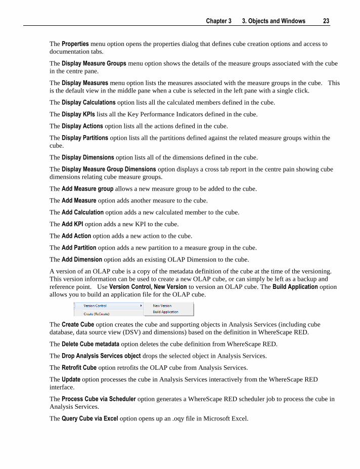
A version of an OLAP cube is a copy of the metadata definition of the cube at the time of the versioning.
This version information can be used to create a new OLAP cube, or can simply be left as a backup and
reference point. Use Version Control, New Version to version an OLAP cube. The Build Application option
allows you to build an application file for the OLAP cube.
The Create Cube option creates the cube and supporting objects in Analysis Services (including cube
database, data source view (DSV) and dimensions) based on the definition in WhereScape RED.
The Delete Cube metadata option deletes the cube definition from WhereScape RED.
The Drop Analysis Services object drops the selected object in Analysis Services.
The Retrofit Cube option retrofits the OLAP cube from Analysis Services.
The Update option processes the cube in Analysis Services interactively from the WhereScape RED
interface.
The Process Cube via Scheduler option generates a WhereScape RED scheduler job to process the cube in
Analysis Services.
The Query Cube via Excel option opens up an .oqy file in Microsoft Excel.
24 3. Objects and Windows
Note: Due to a shortcoming in the Microsoft Office installation it may be necessary to associate the .oqy file
extension with Microsoft Excel before this option will succeed.
The Remove from Project option will remove the cube definition from a user defined RED project.
The Add to Project option will add the cube definition to a user defined RED project.
Check Out is used to mark an object as in use by a developer. It is designed to 'lock' objects that you are
working on so that no one else can alter them until you have checked them back in. Checking out an object
also checks out the indexes and any associated procedures and scripts. Objects may be checked out for a set
period or indefinitely. Once an object is checked out, this menu item changes to Check In. Only the user
who checks out an object can perform the check in action.
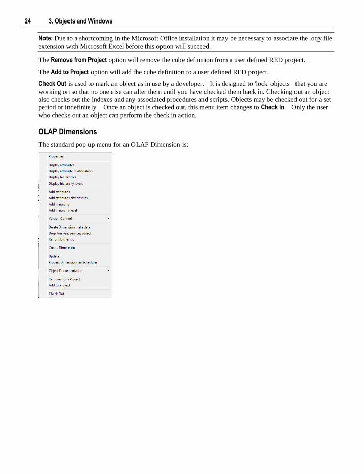
OLAP Dimensions
The standard pop-up menu for an OLAP Dimension is:
Chapter 3 3. Objects and Windows 25
The Properties option displays the OLAP dimension properties dialog which includes documentation tabs.
The Display attributes option lists the attributes for the selected dimension. This is the default view when
an OLAP Dimension is selected in the left pane.
The Display Attribute relationships option shows the relationships between the dimensional attributes.
The Display hierarchies option lists the hierarchies associated with the selected dimension.
The Display hierarchy levels option lists all the levels for all hierarchies for that dimension.
The Add Attributes option adds a new attribute to the dimension.
The Add Attribute relationships option adds an attribute relationship for the selected dimension.
The Add hierarchy option adds a new hierarchy to the dimension.
The Add hierarchy level option adds a level to a hierarchy.
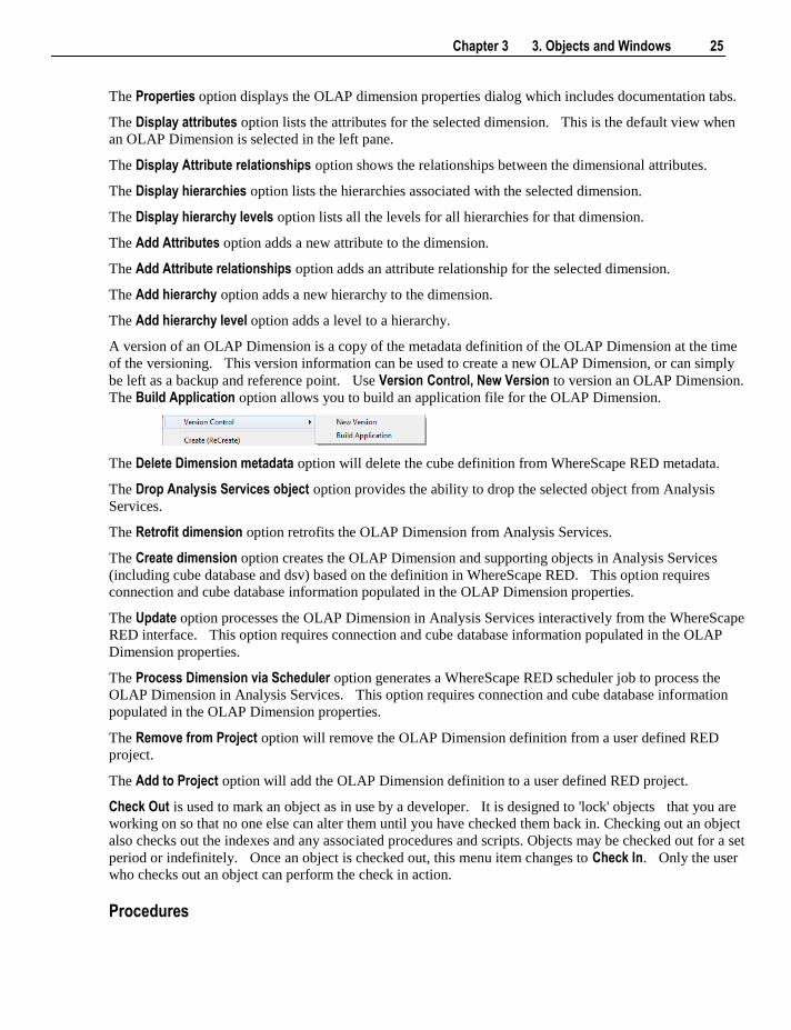
A version of an OLAP Dimension is a copy of the metadata definition of the OLAP Dimension at the time
of the versioning. This version information can be used to create a new OLAP Dimension, or can simply
be left as a backup and reference point. Use Version Control, New Version to version an OLAP Dimension.
The Build Application option allows you to build an application file for the OLAP Dimension.
The Delete Dimension metadata option will delete the cube definition from WhereScape RED metadata.
The Drop Analysis Services object option provides the ability to drop the selected object from Analysis
Services.
The Retrofit dimension option retrofits the OLAP Dimension from Analysis Services.
The Create dimension option creates the OLAP Dimension and supporting objects in Analysis Services
(including cube database and dsv) based on the definition in WhereScape RED. This option requires
connection and cube database information populated in the OLAP Dimension properties.
The Update option processes the OLAP Dimension in Analysis Services interactively from the WhereScape
RED interface. This option requires connection and cube database information populated in the OLAP
Dimension properties.
The Process Dimension via Scheduler option generates a WhereScape RED scheduler job to process the
OLAP Dimension in Analysis Services. This option requires connection and cube database information
populated in the OLAP Dimension properties.
The Remove from Project option will remove the OLAP Dimension definition from a user defined RED
project.
The Add to Project option will add the OLAP Dimension definition to a user defined RED project.
Check Out is used to mark an object as in use by a developer. It is designed to 'lock' objects that you are
working on so that no one else can alter them until you have checked them back in. Checking out an object
also checks out the indexes and any associated procedures and scripts. Objects may be checked out for a set
period or indefinitely. Once an object is checked out, this menu item changes to Check In. Only the user
who checks out an object can perform the check in action.
Procedures
26 3. Objects and Windows
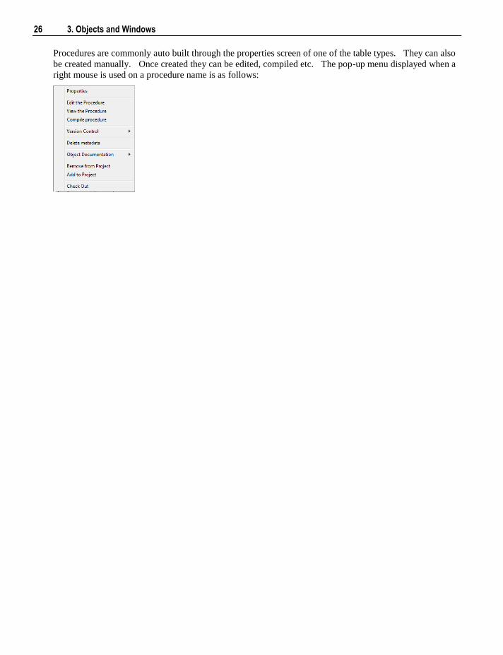
Procedures are commonly auto built through the properties screen of one of the table types. They can also
be created manually. Once created they can be edited, compiled etc. The pop-up menu displayed when a
right mouse is used on a procedure name is as follows:
Chapter 3 3. Objects and Windows 27
If a procedure has been locked as the result of the WhereScape RED utility being killed or failing or a
database failure then it can be unlocked via the properties screen associated with the procedure.
The Edit the Procedure option invokes the procedure editor and loads the procedure. A procedure can be
compiled and executed within the procedure editor.
The View the Procedure menu option displays a read only copy of the procedure. If the procedure is locked
by another user then viewing the procedure is the only option available.
The Compile procedure option will compile the procedure from the metadata.
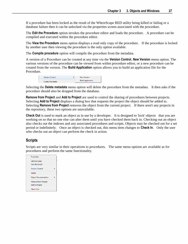
A version of a Procedure can be created at any time via the Version Control, New Version menu option. The
various versions of the procedure can be viewed from within procedure editor, or a new procedure can be
created from the version. The Build Application option allows you to build an application file for the
Procedure.
Selecting the Delete metadata menu option will delete the procedure from the metadata. It then asks if the
procedure should also be dropped from the database.
Remove from Project and Add to Project are used to control the sharing of procedures between projects.
Selecting Add to Project displays a dialog box that requests the project the object should be added to.
Selecting Remove from Project removes the object from the current project. If there aren't any projects in
the repository, these two options are unavailable.
Check Out is used to mark an object as in use by a developer. It is designed to 'lock' objects that you are
working on so that no one else can alter them until you have checked them back in. Checking out an object
also checks out the indexes and any associated procedures and scripts. Objects may be checked out for a set
period or indefinitely. Once an object is checked out, this menu item changes to Check In. Only the user
who checks out an object can perform the check in action.
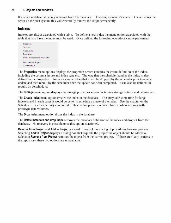
Scripts
Scripts are very similar in their operations to procedures. The same menu options are available as for
procedures and perform the same functionality.
28 3. Objects and Windows
If a script is deleted it is only removed from the metadata. However, as WhereScape RED never stores the
script on the host system, this will essentially remove the script permanently.
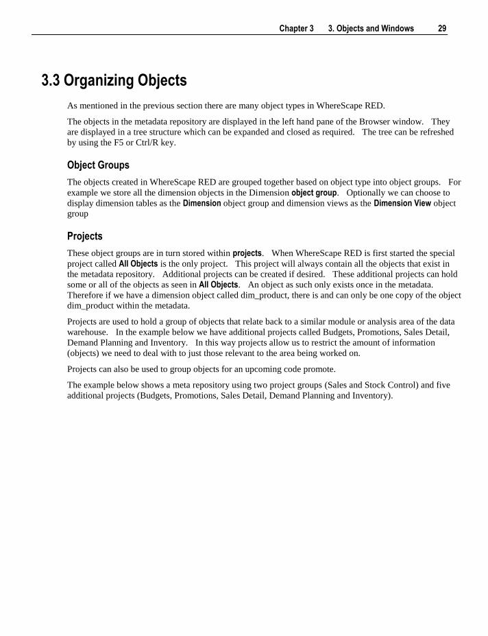
Indexes
Indexes are always associated with a table. To define a new index the menu option associated with the
table that is to have the index must be used. Once defined the following operations can be performed.
The Properties menu options displays the properties screen contains the entire definition of the index,
including the columns in use and index type etc. The way that the scheduler handles the index is also
defined in the Properties. An index can be set so that it will be dropped by the scheduler prior to a table
update and then rebuilt by the scheduler once the update has been completed. It can also be defined for
rebuild on certain days.
The Storage menu option displays the storage properties screen containing storage options and parameters.
The Create Index menu option creates the index in the database. This may take some time for large
indexes, and in such cases it would be better to schedule a create of the index. See the chapter on the
Scheduler if such an activity is required. This menu option is intended for use when working with
prototype data volumes.
The Drop Index menu option drops the index in the database.
The Delete metadata and drop index removes the metadata definition of the index and drops it from the
database. No recovery is possible once this option is actioned.
Remove from Project and Add to Project are used to control the sharing of procedures between projects.
Selecting Add to Project displays a dialog box that requests the project the object should be added to.
Selecting Remove from Project removes the object from the current project. If there aren't any projects in
the repository, these two options are unavailable.
Chapter 3 3. Objects and Windows 29
3.3 Organizing Objects
As mentioned in the previous section there are many object types in WhereScape RED.
The objects in the metadata repository are displayed in the left hand pane of the Browser window. They
are displayed in a tree structure which can be expanded and closed as required. The tree can be refreshed
by using the F5 or Ctrl/R key.
Object Groups
The objects created in WhereScape RED are grouped together based on object type into object groups. For
example we store all the dimension objects in the Dimension object group. Optionally we can choose to
display dimension tables as the Dimension object group and dimension views as the Dimension View object
group
Projects
These object groups are in turn stored within projects. When WhereScape RED is first started the special
project called All Objects is the only project. This project will always contain all the objects that exist in
the metadata repository. Additional projects can be created if desired. These additional projects can hold
some or all of the objects as seen in All Objects. An object as such only exists once in the metadata.
Therefore if we have a dimension object called dim_product, there is and can only be one copy of the object
dim_product within the metadata.
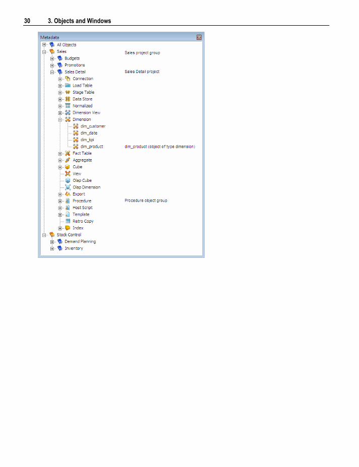
Projects are used to hold a group of objects that relate back to a similar module or analysis area of the data
warehouse. In the example below we have additional projects called Budgets, Promotions, Sales Detail,
Demand Planning and Inventory. In this way projects allow us to restrict the amount of information
(objects) we need to deal with to just those relevant to the area being worked on.
Projects can also be used to group objects for an upcoming code promote.
The example below shows a meta repository using two project groups (Sales and Stock Control) and five
additional projects (Budgets, Promotions, Sales Detail, Demand Planning and Inventory).
30 3. Objects and Windows
Chapter 3 3. Objects and Windows 31
Note: If you delete an object using the right mouse menu, then the object will be deleted from the metadata
and will be removed from all Projects. Remove the object from the project instead of deleting it.
It is important to understand that these projects are only a means of visualizing the objects. Even though
an object may appear in many projects, it only exists once in the metadata.
To create a project, right click in the left pane below the last project and select 'New Project'.
The File / New Project menu option may also be used. Projects can be renamed,removed from the project
group or deleted by using the right mouse menu when positioned on the project name. Deleting a project
does not delete the objects from the metadata, it simply removes their reference in the project being deleted.
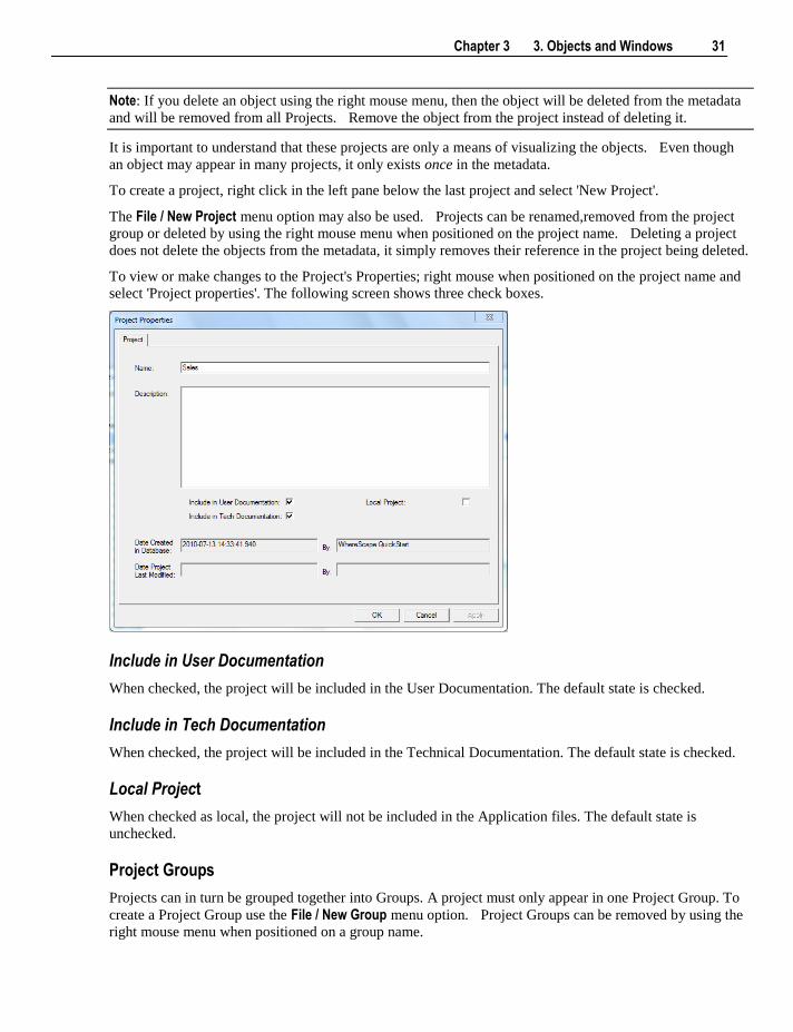
To view or make changes to the Project's Properties; right mouse when positioned on the project name and
select 'Project properties'. The following screen shows three check boxes.
Include in User Documentation
When checked, the project will be included in the User Documentation. The default state is checked.
Include in Tech Documentation
When checked, the project will be included in the Technical Documentation. The default state is checked.
Local Project
When checked as local, the project will not be included in the Application files. The default state is
unchecked.
Project Groups
Projects can in turn be grouped together into Groups. A project must only appear in one Project Group. To
create a Project Group use the File / New Group menu option. Project Groups can be removed by using the
right mouse menu when positioned on a group name.
32 3. Objects and Windows
3.3.1 Adding Objects to Projects There are several different ways to add objects to a project:
Click an object in the left hand pane, type Ctrl/C, click the target project (either the project folder or any
object group or object within it) and type Ctrl/V
Drag the object to the required project
Right click on an object in the left hand pane and choose Add to Project
Highlight a number of objects in the middle pane, right click and choose Add to Project
Using the Project/Object Maintenance Facility (see "3.3.3 Using the Project/Object Maintenance
Facility" on page 34)
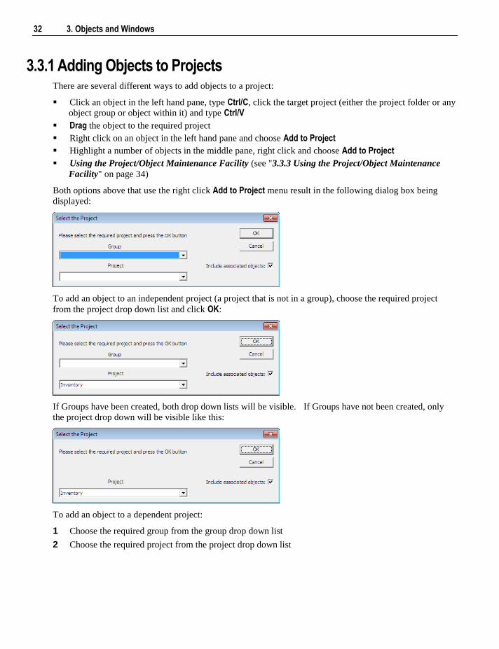
Both options above that use the right click Add to Project menu result in the following dialog box being
displayed:
To add an object to an independent project (a project that is not in a group), choose the required project
from the project drop down list and click OK:
If Groups have been created, both drop down lists will be visible. If Groups have not been created, only
the project drop down will be visible like this:
To add an object to a dependent project:
1 Choose the required group from the group drop down list
2 Choose the required project from the project drop down list
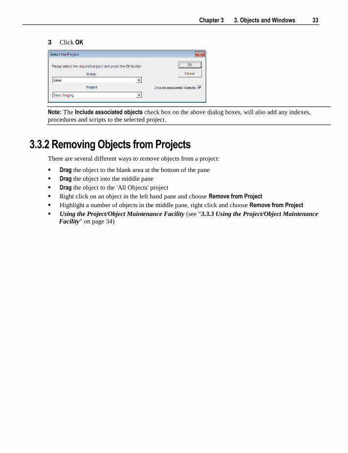
Chapter 3 3. Objects and Windows 33
3 Click OK
Note: The Include associated objects check box on the above dialog boxes, will also add any indexes,
procedures and scripts to the selected project.
3.3.2 Removing Objects from Projects There are several different ways to remove objects from a project:
Drag the object to the blank area at the bottom of the pane
Drag the object into the middle pane
Drag the object to the 'All Objects' project
Right click on an object in the left hand pane and choose Remove from Project
Highlight a number of objects in the middle pane, right click and choose Remove from Project
Using the Project/Object Maintenance Facility (see "3.3.3 Using the Project/Object Maintenance
Facility" on page 34)
34 3. Objects and Windows
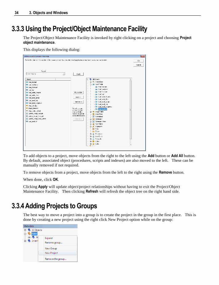
3.3.3 Using the Project/Object Maintenance Facility The Project/Object Maintenance Facility is invoked by right clicking on a project and choosing Project object maintenance.
This displays the following dialog:
To add objects to a project, move objects from the right to the left using the Add button or Add All button.
By default, associated object (procedures, scripts and indexes) are also moved to the left. These can be
manually removed if not required.
To remove objects from a project, move objects from the left to the right using the Remove button.
When done, click OK.
Clicking Apply will update object/project relationships without having to exit the Project/Object
Maintenance Facility. Then clicking Refresh will refresh the object tree on the right hand side.
3.3.4 Adding Projects to Groups The best way to move a project into a group is to create the project in the group in the first place. This is
done by creating a new project using the right click New Project option while on the group:
Chapter 3 3. Objects and Windows 35
The other option is to move an existing project from another group into this group. See Moving Projects
within Groups (see "3.3.6 Moving Projects within Groups" on page 35)
3.3.5 Removing Projects from Groups A project can be removed from a group by:
Dragging the project to the blank area at the bottom of the pane
Dragging the project into the middle pane
Dragging the project to the 'All Objects' project
Removing the project using right click Remove Project from Group
Deleting the project using right click Delete Project
Note: The first four methods move the project out from the group to become an independent project. The
last option removes the project from the metadata repository.
3.3.6 Moving Projects within Groups
Note: An object can be in any number of projects, but a project can only be in one Group.
Performing a drag from one group to another group will simply create an additional project->group
mapping.
To move a project from one group to another group:
1 'Copy' the project by dragging the project from the one group to the other group.
2 Remove the project from the original group by right clicking and selecting Remove Project from Group.
3.4 Windows and Panes
WhereScape RED has a number of different windows that are utilized in the building and maintenance of a
data warehouse. Each window may in some cases be broken into panes. There are four main windows
that are used extensively in the building of a data warehouse. These are the Browser window, the
Scheduler window, the Diagrammatical window and the Procedure Editor window.
36 3. Objects and Windows
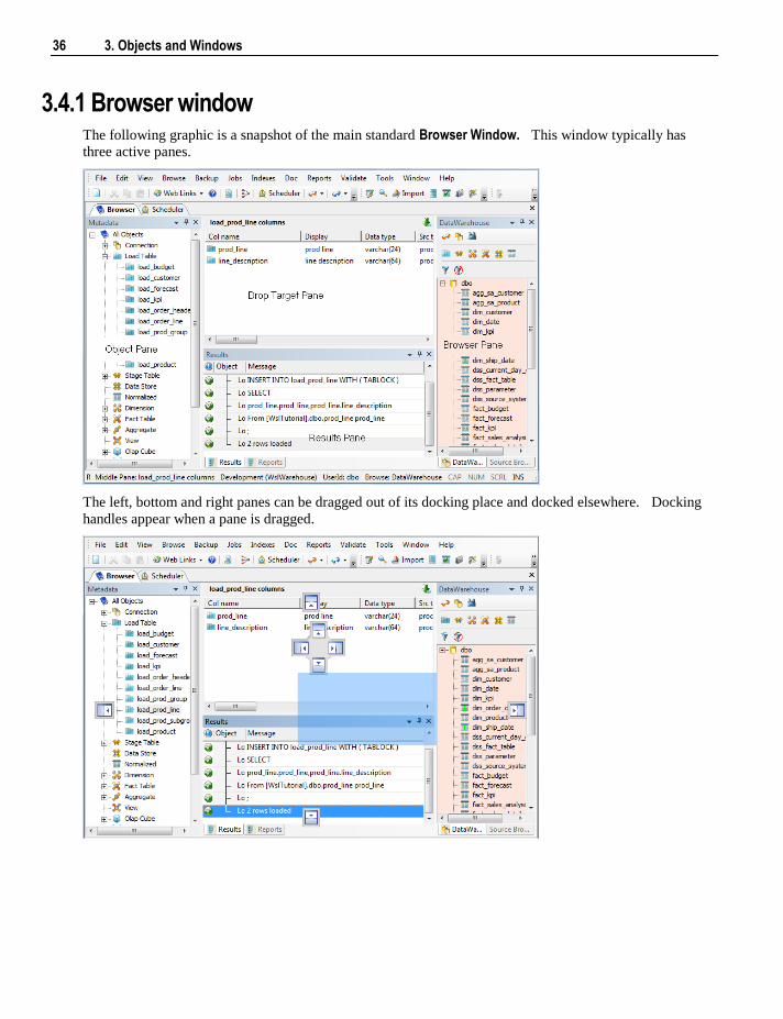
3.4.1 Browser window The following graphic is a snapshot of the main standard Browser Window. This window typically has
three active panes.
The left, bottom and right panes can be dragged out of its docking place and docked elsewhere. Docking
handles appear when a pane is dragged.
Chapter 3 3. Objects and Windows 37
The left most pane contains all the objects within the metadata repository. These objects are stored in
object groups (e.g. Dimension ). The object groups are in turn optionally stored in Projects, and the
Projects are optionally stored within Project Groups.
The middle pane is used to show the results of various queries on both the metadata and the underlying
source and database tables. The middle pane is also used as the drop target in drag and drop operations.
The status line at the bottom of the screen displays the current contents of the middle pane.
The right hand pane is the browser pane and it shows source systems. There are two browser panes
available at any one time. This source may be the data warehouse itself. Typically this pane is used as the
source of information in the drag and drop operations. The status line at the bottom of the screen displays
the connection used in this right hand pane.
The bottom pane is the results pane. It shows the results of any command executed in the tool. The
messages are related to an object, multiple messages can show as a result of a command executed for an
object. Expand the '+' sign next to an object to see a complete list of messages relating to an object. When
a report is run from the main menu, the results are displayed in a separate tab in the bottom pane.
Pop-up menus are available in all four panes.
F5 or Ctrl/R can be used to refresh the left and right hand panes, when the cursor is positioned within these
panes.
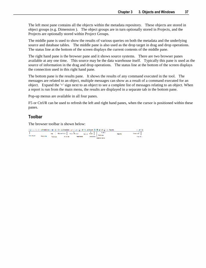
Toolbar
The browser toolbar is shown below:
38 3. Objects and Windows
The diagrammatical view button (diagram view) switches to the diagrammatical window. This window
allows the representation and printing of star schema and track back diagrams.
The scheduler button switches to the scheduler control window.
The two source browse buttons (one orange and one blue) allow a quick method of invoking the source
browser which populates the 'Browser pane'. Each of the two browse buttons, when chosen, browses to the
connection last used for that button. To change the connection being browsed click the down arrow beside
the glasses icon.
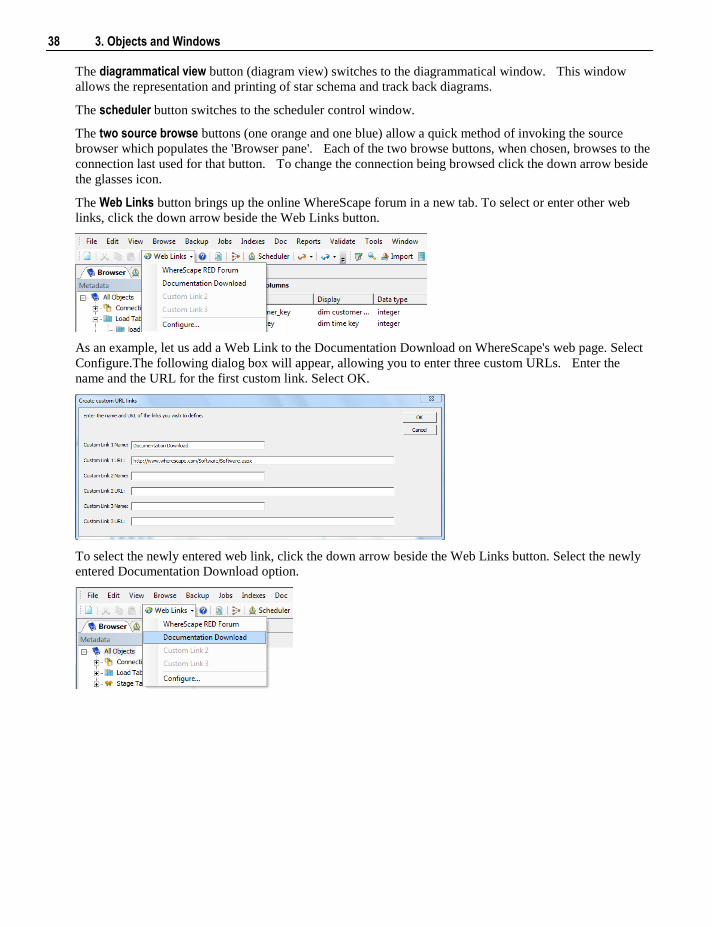
The Web Links button brings up the online WhereScape forum in a new tab. To select or enter other web
links, click the down arrow beside the Web Links button.
As an example, let us add a Web Link to the Documentation Download on WhereScape's web page. Select
Configure.The following dialog box will appear, allowing you to enter three custom URLs. Enter the
name and the URL for the first custom link. Select OK.
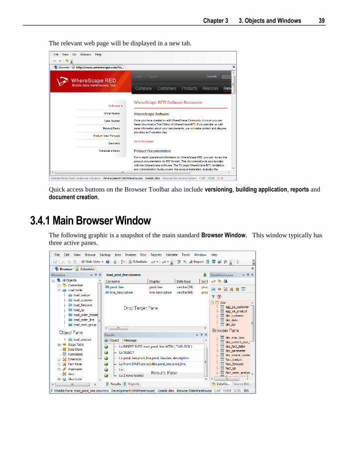
To select the newly entered web link, click the down arrow beside the Web Links button. Select the newly
entered Documentation Download option.
Chapter 3 3. Objects and Windows 39
The relevant web page will be displayed in a new tab.
Quick access buttons on the Browser Toolbar also include versioning, building application, reports and
document creation.
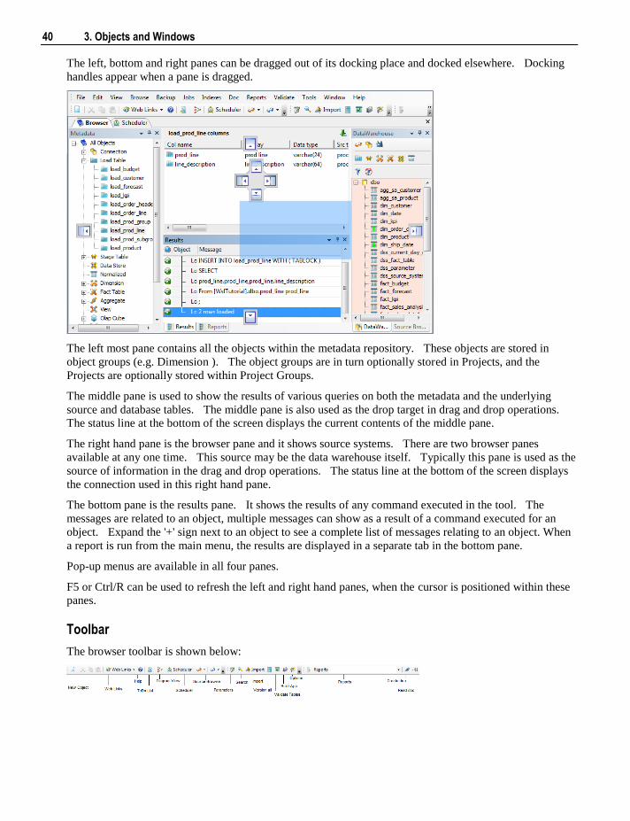
3.4.1 Main Browser Window The following graphic is a snapshot of the main standard Browser Window. This window typically has
three active panes.
40 3. Objects and Windows
The left, bottom and right panes can be dragged out of its docking place and docked elsewhere. Docking
handles appear when a pane is dragged.
The left most pane contains all the objects within the metadata repository. These objects are stored in
object groups (e.g. Dimension ). The object groups are in turn optionally stored in Projects, and the
Projects are optionally stored within Project Groups.
The middle pane is used to show the results of various queries on both the metadata and the underlying
source and database tables. The middle pane is also used as the drop target in drag and drop operations.
The status line at the bottom of the screen displays the current contents of the middle pane.
The right hand pane is the browser pane and it shows source systems. There are two browser panes
available at any one time. This source may be the data warehouse itself. Typically this pane is used as the
source of information in the drag and drop operations. The status line at the bottom of the screen displays
the connection used in this right hand pane.
The bottom pane is the results pane. It shows the results of any command executed in the tool. The
messages are related to an object, multiple messages can show as a result of a command executed for an
object. Expand the '+' sign next to an object to see a complete list of messages relating to an object. When
a report is run from the main menu, the results are displayed in a separate tab in the bottom pane.
Pop-up menus are available in all four panes.
F5 or Ctrl/R can be used to refresh the left and right hand panes, when the cursor is positioned within these
panes.
Toolbar
The browser toolbar is shown below:
Chapter 3 3. Objects and Windows 41
The diagrammatical view button (diagram view) switches to the diagrammatical window. This window
allows the representation and printing of star schema and track back diagrams.
The scheduler button switches to the scheduler control window.
The two source browse buttons (one orange and one blue) allow a quick method of invoking the source
browser which populates the 'Browser pane'. Each of the two browse buttons, when chosen, browses to the
connection last used for that button. To change the connection being browsed click the down arrow beside
the glasses icon.
The Web Links button brings up the online WhereScape forum in a new tab. To select or enter other web
links, click the down arrow beside the Web Links button.
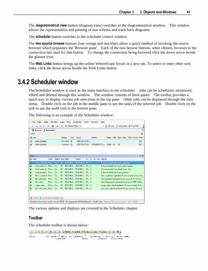
3.4.2 Scheduler window The Scheduler window is used as the main interface to the scheduler. Jobs can be scheduled, monitored,
edited and deleted through this window. The window consists of three panes. The toolbar provides a
quick way to display various job selections in the top pane. Other jobs can be displayed through the Jobs
menu. Double click on the job in the middle pane to see the tasks of the selected job. Double click on the
task to see the audit trail in the bottom pane.
The following is an example of the Scheduler window:
The various options and displays are covered in the Scheduler chapter.
Toolbar
The scheduler toolbar is shown below:
42 3. Objects and Windows
The new job button invokes the dialog to create a new scheduled job. The browser window button
switches back to the main browser window. The auto refresh button, when depressed, will result in a
refresh of the current (right pane) display every 10 seconds. Click the button again to stop the auto refresh.
The refresh interval can be adjusted through the menu option Auto/Refresh interval. Quick access to
different categories of jobs are also available via the toolbar.
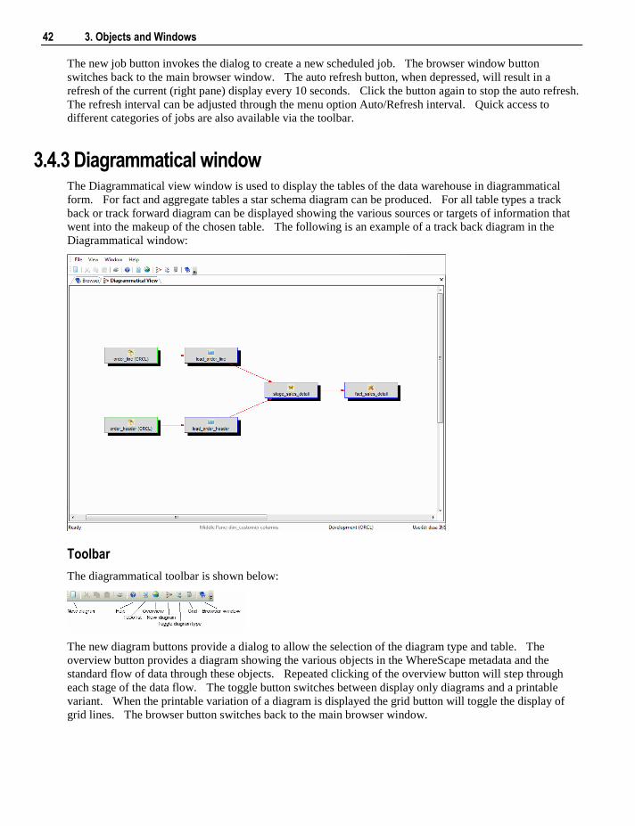
3.4.3 Diagrammatical window The Diagrammatical view window is used to display the tables of the data warehouse in diagrammatical
form. For fact and aggregate tables a star schema diagram can be produced. For all table types a track
back or track forward diagram can be displayed showing the various sources or targets of information that
went into the makeup of the chosen table. The following is an example of a track back diagram in the
Diagrammatical window:
Toolbar
The diagrammatical toolbar is shown below:
The new diagram buttons provide a dialog to allow the selection of the diagram type and table. The
overview button provides a diagram showing the various objects in the WhereScape metadata and the
standard flow of data through these objects. Repeated clicking of the overview button will step through
each stage of the data flow. The toggle button switches between display only diagrams and a printable
variant. When the printable variation of a diagram is displayed the grid button will toggle the display of
grid lines. The browser button switches back to the main browser window.
Chapter 3 3. Objects and Windows 43
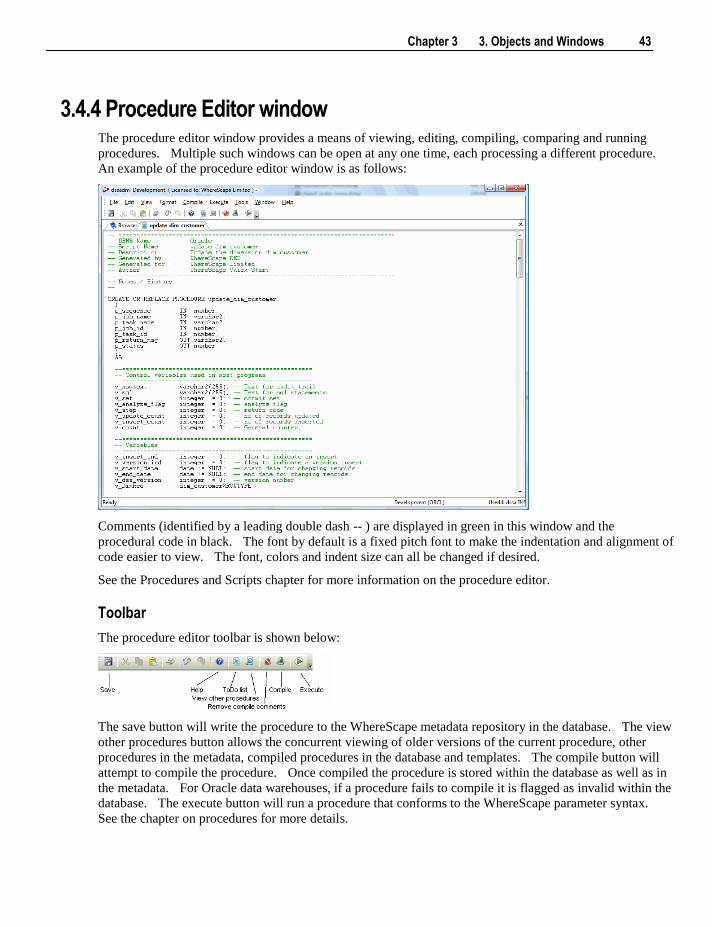
3.4.4 Procedure Editor window The procedure editor window provides a means of viewing, editing, compiling, comparing and running
procedures. Multiple such windows can be open at any one time, each processing a different procedure.
An example of the procedure editor window is as follows:
Comments (identified by a leading double dash -- ) are displayed in green in this window and the
procedural code in black. The font by default is a fixed pitch font to make the indentation and alignment of
code easier to view. The font, colors and indent size can all be changed if desired.
See the Procedures and Scripts chapter for more information on the procedure editor.
Toolbar
The procedure editor toolbar is shown below:
The save button will write the procedure to the WhereScape metadata repository in the database. The view
other procedures button allows the concurrent viewing of older versions of the current procedure, other
procedures in the metadata, compiled procedures in the database and templates. The compile button will
attempt to compile the procedure. Once compiled the procedure is stored within the database as well as in
the metadata. For Oracle data warehouses, if a procedure fails to compile it is flagged as invalid within the
database. The execute button will run a procedure that conforms to the WhereScape parameter syntax.
See the chapter on procedures for more details.
44 3. Objects and Windows
3.5 Database Error Messages
From time to time a SQL error may be raised by WhereScape RED.
These are usually cause by the data warehouse database returning an error.
There are many causes of database error messages being returned to RED. The most common include
permission issues and invalid SQL statements being run.
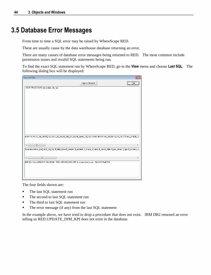
To find the exact SQL statement run by WhereScape RED, go to the View menu and choose Last SQL. The
following dialog box will be displayed:
The four fields shown are:
The last SQL statement run
The second to last SQL statement run
The third to last SQL statement run
The error message (if any) from the last SQL statement
In the example above, we have tried to drop a procedure that does not exist. IBM DB2 returned an error
telling us RED.UPDATE_DIM_KPI does not exist in the database.
Chapter 4 4. Tutorials 45
The WhereScape RED tutorials are located in the WhereScape RED Tutorial Help.
C H A P T E R 4
4. Tutorials

Chapter 5 5. Settings and Parameters 47
This chapter describes the settings and default values that can be made for a metadata repository. The
concept of parameters is also covered. Parameters are the methodology used in the WhereScape RED tool
set to allow communication between WhereScape RED and the various procedures.
In This Chapter
5.1 Default Settings ..................................................................... 47
5.2 Parameters ............................................................................. 72
5.1 Default Settings
This chapter describes how to set the default behavior and naming standards in WhereScape RED. The
following defaults are covered:
Repository Attributes and Options
Object Options
Table, Index and Key Name Defaults
Procedure Naming Defaults
Tablespace and Filegroup Defaults
Ancillary Table and Column Defaults
Icon Settings
Documentation Settings
Statistic Settings
WhereScape RED makes use of two metadata tables and a number of columns to assist in the development
and operation of the data warehouse. These tables and columns are discussed along with the options for
their use and the changing of the default values.
C H A P T E R 5
5. Settings and Parameters
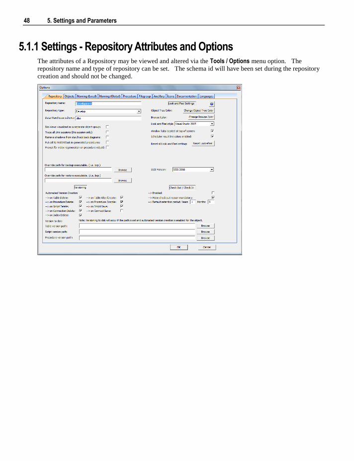
48 5. Settings and Parameters
5.1.1 Settings - Repository Attributes and Options The attributes of a Repository may be viewed and altered via the Tools / Options menu option. The
repository name and type of repository can be set. The schema id will have been set during the repository
creation and should not be changed.
Chapter 5 5. Settings and Parameters 49
Repository Name
The repository name can be set. This appears in the top left hand corner of the title bar in WhereScape
RED. Restart WhereScape RED for repository name changes to take affect.
Repository Type
The repository type should reflect the environment. For example a 'Production' type should be chosen for
the production environment. A color is associated with each repository type. These colors tint the left
hand pane of both the main browser window and the scheduler window. The colors can be changed on a
specific PC by changing the object tree color (see below).
Data Warehouse schema
The schema of the data warehouse is used by the WhereScape RED scheduler. You should not normally
need to change this value.
Views visualized as a separate object group
This check box will display a new object group called Views where all view objects are stored. The
default (unchecked) state is that views are part of the dimension object group and are considered dimension
views. WhereScape RED will have to be exited and restarted to see the impact of this change. This
setting is only relevant for the PC on which the setting is made. (i.e. it is not a global setting for the
repository).
Trace Unix sessions
This check box when set will trace all Unix activity undertaken by the WhereScape RED program until
terminated. The file WslMedTelnet.txt will be created in the program directory for WhereScape RED.
This option is intended for debugging of specific Unix problems and the setting of this switch would
normally be done at the request of WhereScape when attempting to solve a Telnet issue. This setting is
only relevant for the PC on which the setting is made. (i.e. it is not a global setting for the repository).
Remove shadows from star / track back diagrams
This check box when set will prevent a shadow appearing on all printable diagrams produced in the
diagrammatical window.
Put call to WsWrkTask in generated procedures
This check box when set will result in a call to the WsWrkTask function being placed at the end of most of
the generated update procedures. These calls to WsWrkTask result in counters being set in the meta table
ws_wrk_task_log. These counters can be viewed via a query on the view ws_admin_v_task.
Prompt for index regeneration on procedure rebuild
This check box when set, results in WhereScape RED prompting for index regeneration whenever an
update procedure is rebuilt.
Scheduler database logon uses Authenticated User
This option should be enabled if the scheduler is running under an operating system authenticated user.
This option is only available in Oracle.
50 5. Settings and Parameters
Override path for Backup executable
By default WhereScape RED tries to find the path of the backup executable. This is bcp.exe for SQL
Server, exp.exe for Oracle and db2cmd.exe for IBM DB2. This edit box provides the ability to specify the
exact location and name of the executable. This is useful when WhereScape RED cannot find the program
or if there are multiple versions of the program on the PC.
Override path for Restore executable
By default WhereScape RED tries to find the path of the restore executable. This is bcp.exe for SQL
Server, imp.exe for Oracle and db2cmd.exe for IBM DB2. This edit box provides the ability to specify the
exact location and name of the executable. This is useful when WhereScape RED cannot find the program
or if there are multiple versions of the program on the PC.
SSIS Version
Select the relevant version of SQL Server Integration Services from the drop down list.
Versioning
A number of check boxes exist to enable the selection of automated versioning of objects. The first group
of five check boxes will version an object prior to its deletion. If all five boxes are set then every type of
object will be versioned prior to deletion. These five check boxes are normally set by default. The table
delete option also covers cube deletion.
The remaining four check boxes should normally be set in a production environment at the very least.
They generate a version whenever a change is made that affects the data warehouse.
If the data warehouse is viewed as a series of tables, procedures and scripts then whenever one of these
elements is changed a new version of the element (object) is created.
Version to disk
If any of the three version to disk paths are set, WhereScape RED will automatically create ascii files
containing the applicable ddl or code each time an automated version occurs in the entered directory.
Look and Feel Settings
The Object Tree Color dialog allows the setting of the color of the left hand pane in the main browser
window. The color can be set for each repository type. For example in your production repository this
could be set to a light red to provide a visual reminder that the user is in the production environment. Any
changes made are for the local PC only. All other users will continue to get the default color scheme.
The Browse Color dialog sets the default color for the right hand pane in the main browser window when
the data warehouse connection is being browsed. It gives the ability to provide a visual reminder that the
data warehouse is being browsed.
The Look and Feel style drop down provides several different options for the look and feel of WhereScape
RED based on different available windows styles.
De-select the check box Window Tabs location at top of screen to change the tab location for the browser,
scheduler, etc to the size of the display.
The Scheduler result line color enabled check box can be enabled to turn on job status color coding in the
scheduler.
Chapter 5 5. Settings and Parameters 51
To reset the appearance of WhereScape RED to the defaults, click the Reset all Look and Feel settings
button and restart WhereScape RED.
Check Out and Check In
Click on the Enabled check box to enable check in and check out in WhereScape RED. By choosing Make check out reason mandatory, developers are required to enter a check out reason. The Default retention period can be set in years and/or months.
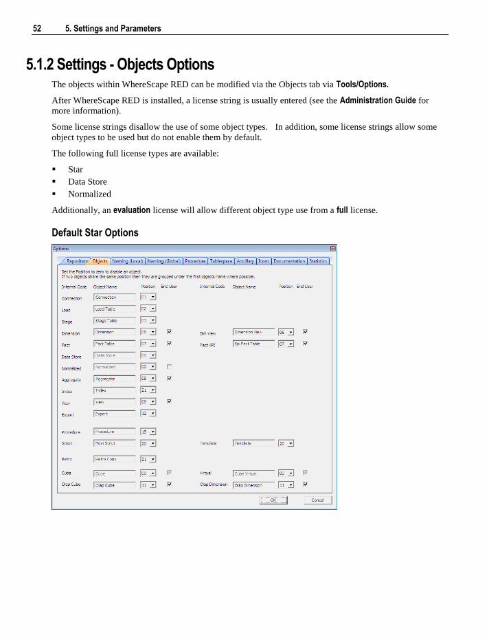
52 5. Settings and Parameters
5.1.2 Settings - Objects Options The objects within WhereScape RED can be modified via the Objects tab via Tools/Options.
After WhereScape RED is installed, a license string is usually entered (see the Administration Guide for
more information).
Some license strings disallow the use of some object types. In addition, some license strings allow some
object types to be used but do not enable them by default.
The following full license types are available:
Star
Data Store
Normalized
Additionally, an evaluation license will allow different object type use from a full license.
Default Star Options
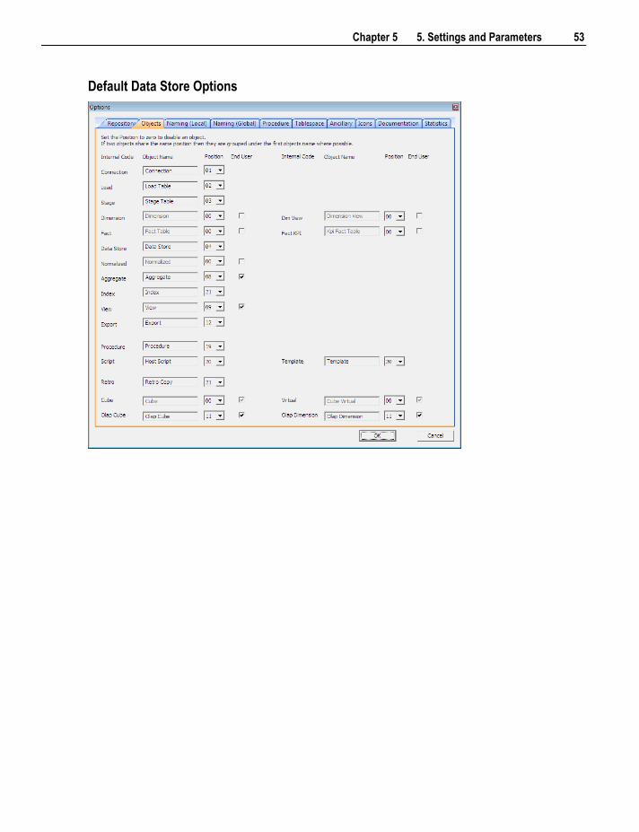
Chapter 5 5. Settings and Parameters 53
Default Data Store Options
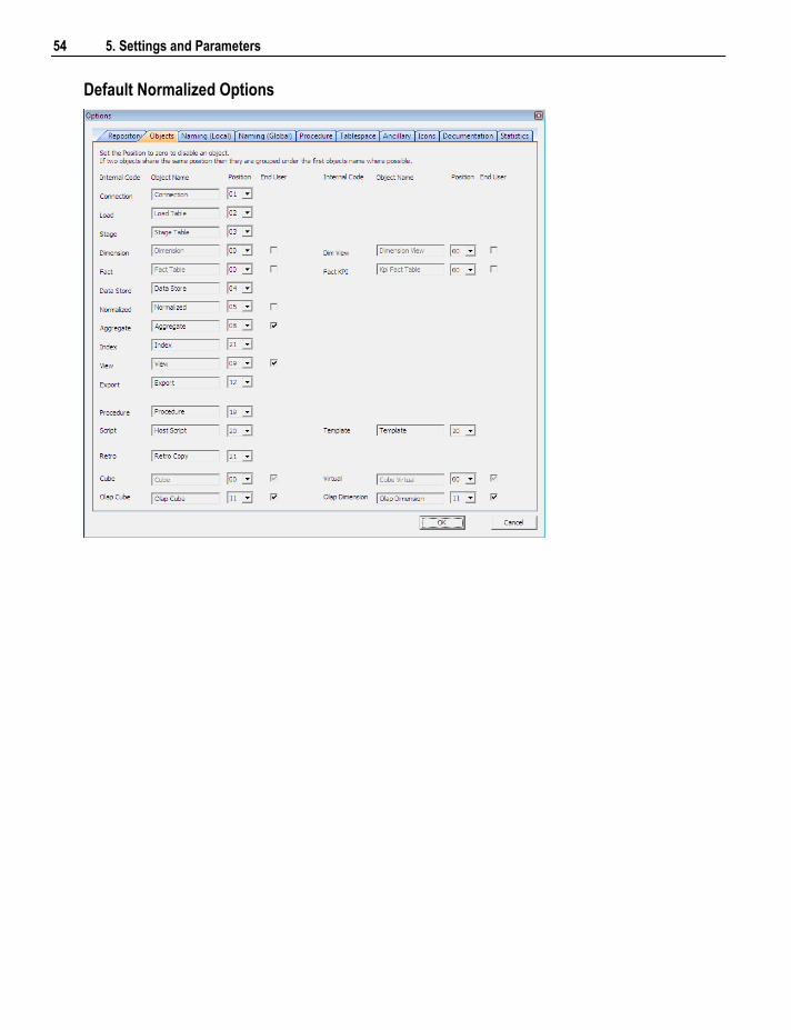
54 5. Settings and Parameters
Default Normalized Options
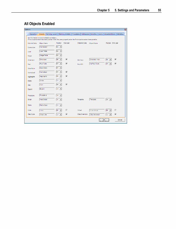
Chapter 5 5. Settings and Parameters 55
All Objects Enabled
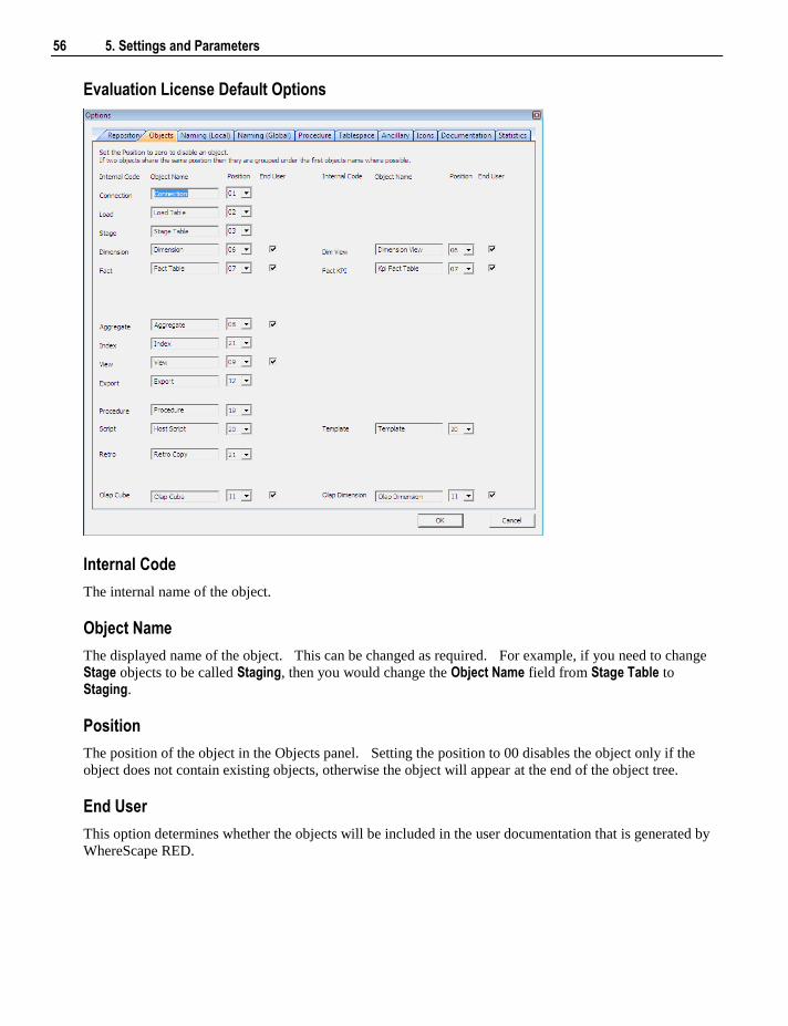
56 5. Settings and Parameters
Evaluation License Default Options
Internal Code
The internal name of the object.
Object Name
The displayed name of the object. This can be changed as required. For example, if you need to change
Stage objects to be called Staging, then you would change the Object Name field from Stage Table to
Staging.
Position
The position of the object in the Objects panel. Setting the position to 00 disables the object only if the
object does not contain existing objects, otherwise the object will appear at the end of the object tree.
End User
This option determines whether the objects will be included in the user documentation that is generated by
WhereScape RED.
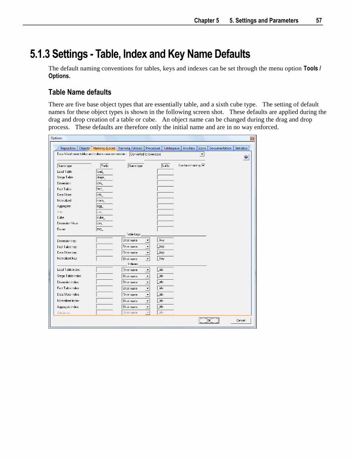
Chapter 5 5. Settings and Parameters 57
5.1.3 Settings - Table, Index and Key Name Defaults The default naming conventions for tables, keys and indexes can be set through the menu option Tools / Options.
Table Name defaults
There are five base object types that are essentially table, and a sixth cube type. The setting of default
names for these object types is shown in the following screen shot. These defaults are applied during the
drag and drop creation of a table or cube. An object name can be changed during the drag and drop
process. These defaults are therefore only the initial name and are in no way enforced.
58 5. Settings and Parameters
A prefix and/or a suffix string can be applied to an object name. Within Oracle and IBM DB2, a table
name may be a maximum of 30 characters long, so these pre and post fix strings should not be more than
eight characters long (WhereScape RED short names are a maximum of 22 long in Oracle and SQL Server
and 12 long in DB2).
From the example screen above, if a source table called 'customer' (with a short name of 'customer') was
dragged into a load table drop target then the default name would be 'load_customer'.
The object name defaults shown above are the values that are installed with the base metadata. They can
be changed at any stage, however, the change does not affect any existing objects. So, if a new naming
regime is chosen any existing objects will need to be renamed through the properties screen of the object.
Table and column case
WhereScape RED will automatically convert the case of table and column names when dragging from a
source system. The default is to convert all table and column names to lower case. This case conversion
setting is defined for the current computer only, as a local setting. Note that all Oracle table and column
names are upper case by default.
Global and local settings
Table name defaults can either be saved globally (in the database) or locally (on the current computer).
Choose the appropriate tabs Naming (Local) or Naming(Global) to save locally or globally.
Artificial Key name defaults
During the drag and drop generation of new dimension and fact tables, WhereScape RED will build an
artificial (surrogate) key for the table. The naming convention for that key can be set through the same
menu option as above. As well as potential pre-fix and suffix values, we also need to choose between the
inclusion of the full table name, or the short name assigned to each table.
In the example screen above, which is the default, a dimension table key would use the table short name and
have a suffix of "_key". So our load_customer table example would generate a key called
dim_customer_key if it where dragged into a dimension drop target.
Index name defaults
Whenever a new procedure is defined, WhereScape RED builds or rebuilds a standard set of indexes for the
table. These indexes will be created using the standard defined. As with the key naming we can set either
a pre-fix or suffix value, or in fact both, as well as choosing the use of either the table name or the short
name associated with the table.
In addition to the naming specifications above WhereScape RED will add up to a further 3 characters to the
end of the index name. These additional values will be "_0" through "_99", or "_A" through "_Z", or
"_SC". When a new index is manually added it will have the additional value of "_x" by default. This
should be changed. The WhereScape RED naming standard for indexes is described below, but any valid
name may be used.
From the example screen above, a fact table would have indexes generated using the short name and with a
suffix of "_idx". Therefore a fact_sales fact table would have indexes such as fact_sales_idx_x.
Ultimate suffix meaning
_0 artificial key
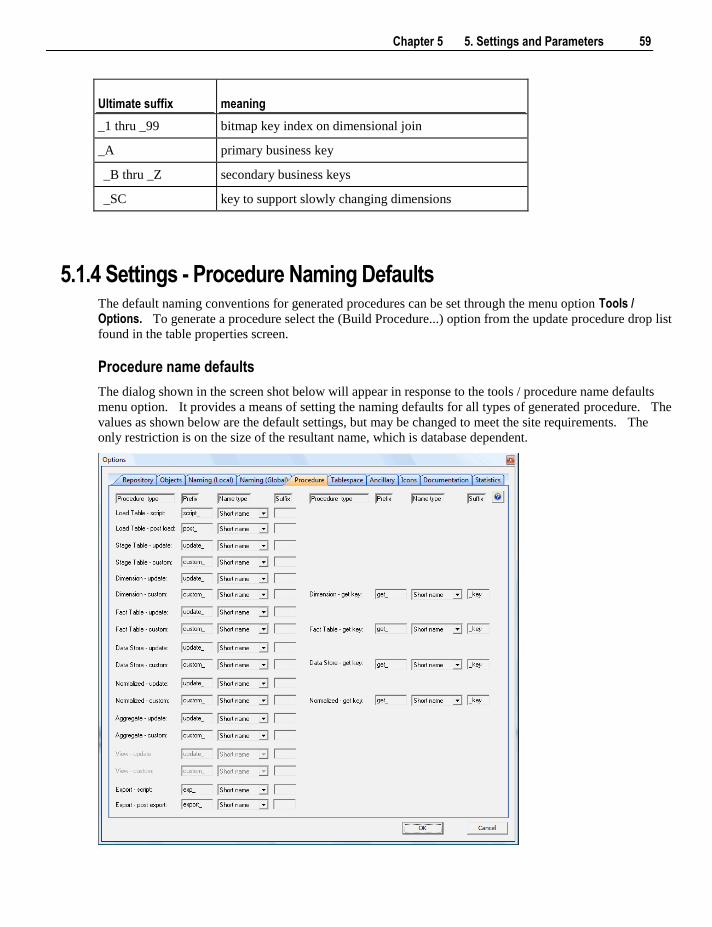
Chapter 5 5. Settings and Parameters 59
Ultimate suffix meaning
_1 thru _99 bitmap key index on dimensional join
_A primary business key
_B thru _Z secondary business keys
_SC key to support slowly changing dimensions
5.1.4 Settings - Procedure Naming Defaults The default naming conventions for generated procedures can be set through the menu option Tools / Options. To generate a procedure select the (Build Procedure...) option from the update procedure drop list
found in the table properties screen.
Procedure name defaults
The dialog shown in the screen shot below will appear in response to the tools / procedure name defaults
menu option. It provides a means of setting the naming defaults for all types of generated procedure. The
values as shown below are the default settings, but may be changed to meet the site requirements. The
only restriction is on the size of the resultant name, which is database dependent.
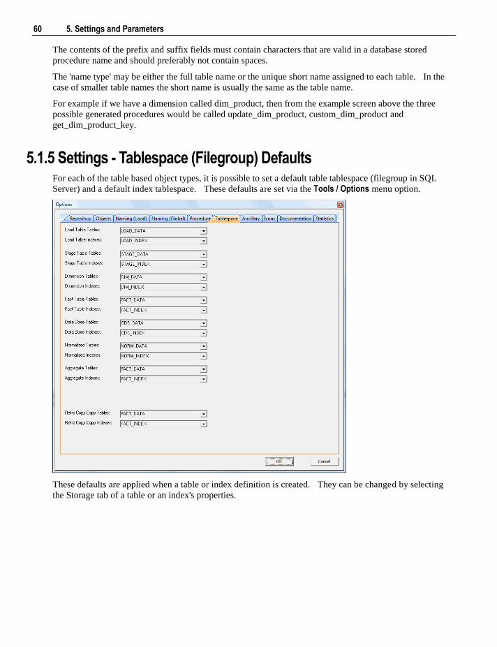
60 5. Settings and Parameters
The contents of the prefix and suffix fields must contain characters that are valid in a database stored
procedure name and should preferably not contain spaces.
The 'name type' may be either the full table name or the unique short name assigned to each table. In the
case of smaller table names the short name is usually the same as the table name.
For example if we have a dimension called dim_product, then from the example screen above the three
possible generated procedures would be called update_dim_product, custom_dim_product and
get_dim_product_key.
5.1.5 Settings - Tablespace (Filegroup) Defaults For each of the table based object types, it is possible to set a default table tablespace (filegroup in SQL
Server) and a default index tablespace. These defaults are set via the Tools / Options menu option.
These defaults are applied when a table or index definition is created. They can be changed by selecting
the Storage tab of a table or an index's properties.
Chapter 5 5. Settings and Parameters 61
5.1.6 Settings - Ancillary Table and Column Defaults When building the data warehouse WhereScape RED makes use of a number of special tables and columns.
Two tables are used. These are called by default dss_source_system and dss_fact_table and are discussed
in detail in the sections below.
The special columns used are defined in the table below.
Column name description
dss_source_system_key
Added to support dimensions that cannot be fully conformed, and
the inclusion of subsequent source systems. See the section
below for more details.
dss_fact_table_key Used in composite rollup fact tables to identify the source fact
table that contributed the particular row.
dss_create_time Indicates when a dimension record was created.
dss_update_time Indicates when the record was last updated in the data warehouse.
Used in the updating of rollup fact tables and aggregate tables.
dss_count Applied to fact tables. Provides a simple row count variable that
can be used by end user tools.
dss_current_flag Used for slowly changing dimensions. This flag identifies the
current record where multiple versions exist.
dss_version Used for slowly changing dimensions. This column contains the
version number of a dimension record. Numbered from 1
upwards with the highest number being the latest or current
version. It forms part of the unique constraint for the business
key of a slowly changing dimension.
dss_start_date Used for slowly changing dimensions. This column provides a
date time stamp when the dimension record began life. If null
then it was the first record. It is used to ascertain which
dimension record should be used when multiple are available.
dss_end_date Used for slowly changing dimensions. This column provides a
date time stamp when the dimension record ceased to be the
current record. It is used to ascertain which dimension record
should be used when multiple are available.
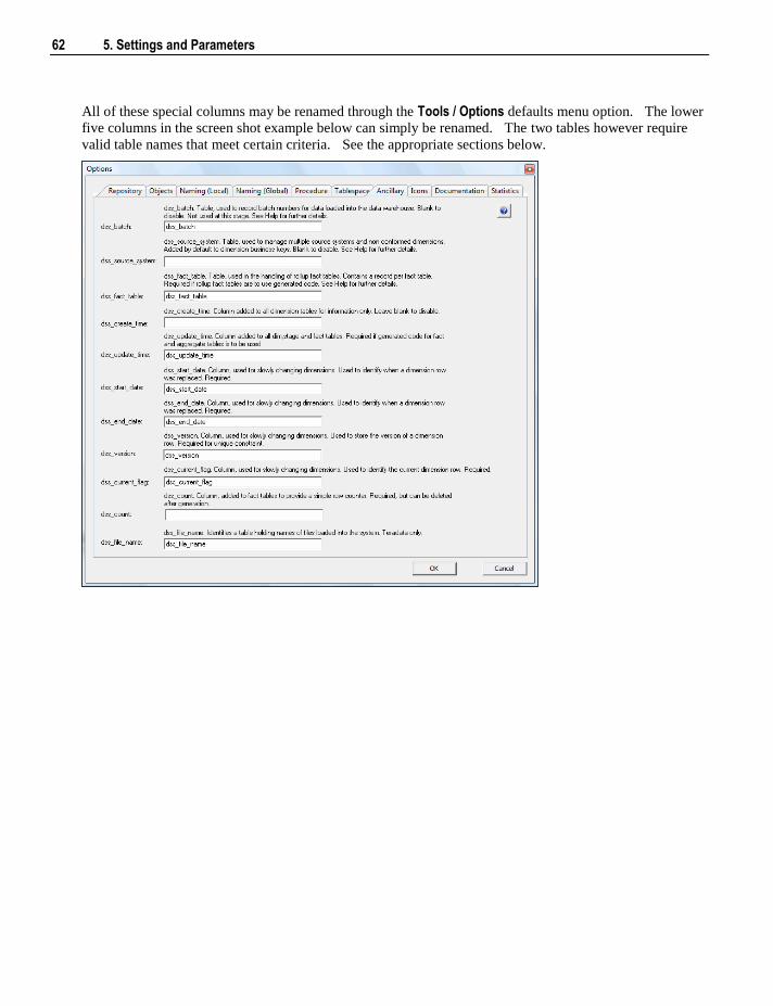
62 5. Settings and Parameters
All of these special columns may be renamed through the Tools / Options defaults menu option. The lower
five columns in the screen shot example below can simply be renamed. The two tables however require
valid table names that meet certain criteria. See the appropriate sections below.
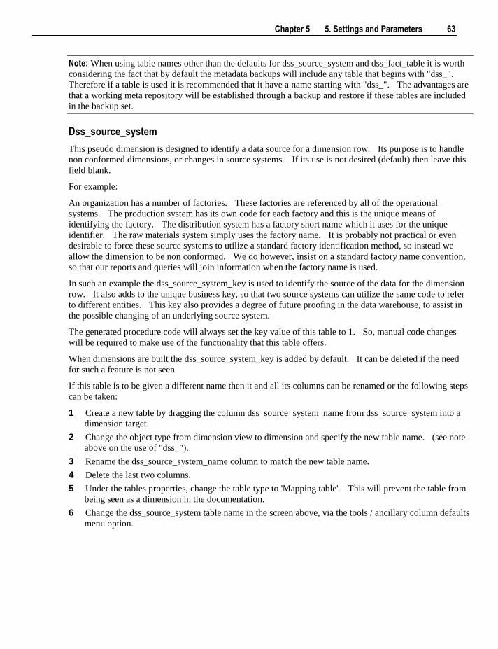
Chapter 5 5. Settings and Parameters 63
Note: When using table names other than the defaults for dss_source_system and dss_fact_table it is worth
considering the fact that by default the metadata backups will include any table that begins with "dss_".
Therefore if a table is used it is recommended that it have a name starting with "dss_". The advantages are
that a working meta repository will be established through a backup and restore if these tables are included
in the backup set.
Dss_source_system
This pseudo dimension is designed to identify a data source for a dimension row. Its purpose is to handle
non conformed dimensions, or changes in source systems. If its use is not desired (default) then leave this
field blank.
For example:
An organization has a number of factories. These factories are referenced by all of the operational
systems. The production system has its own code for each factory and this is the unique means of
identifying the factory. The distribution system has a factory short name which it uses for the unique
identifier. The raw materials system simply uses the factory name. It is probably not practical or even
desirable to force these source systems to utilize a standard factory identification method, so instead we
allow the dimension to be non conformed. We do however, insist on a standard factory name convention,
so that our reports and queries will join information when the factory name is used.
In such an example the dss_source_system_key is used to identify the source of the data for the dimension
row. It also adds to the unique business key, so that two source systems can utilize the same code to refer
to different entities. This key also provides a degree of future proofing in the data warehouse, to assist in
the possible changing of an underlying source system.
The generated procedure code will always set the key value of this table to 1. So, manual code changes
will be required to make use of the functionality that this table offers.
When dimensions are built the dss_source_system_key is added by default. It can be deleted if the need
for such a feature is not seen.
If this table is to be given a different name then it and all its columns can be renamed or the following steps
can be taken:
1 Create a new table by dragging the column dss_source_system_name from dss_source_system into a
dimension target.
2 Change the object type from dimension view to dimension and specify the new table name. (see note
above on the use of "dss_").
3 Rename the dss_source_system_name column to match the new table name.
4 Delete the last two columns.
5 Under the tables properties, change the table type to 'Mapping table'. This will prevent the table from
being seen as a dimension in the documentation.
6 Change the dss_source_system table name in the screen above, via the tools / ancillary column defaults
menu option.
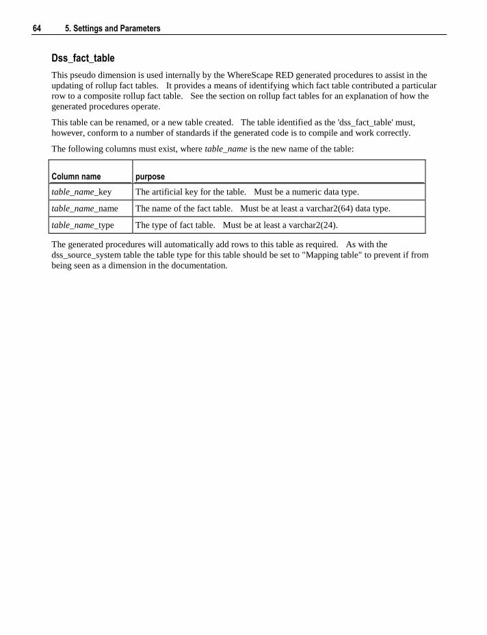
64 5. Settings and Parameters
Dss_fact_table
This pseudo dimension is used internally by the WhereScape RED generated procedures to assist in the
updating of rollup fact tables. It provides a means of identifying which fact table contributed a particular
row to a composite rollup fact table. See the section on rollup fact tables for an explanation of how the
generated procedures operate.
This table can be renamed, or a new table created. The table identified as the 'dss_fact_table' must,
however, conform to a number of standards if the generated code is to compile and work correctly.
The following columns must exist, where table_name is the new name of the table:
Column name purpose
table_name_key The artificial key for the table. Must be a numeric data type.
table_name_name The name of the fact table. Must be at least a varchar2(64) data type.
table_name_type The type of fact table. Must be at least a varchar2(24).
The generated procedures will automatically add rows to this table as required. As with the
dss_source_system table the table type for this table should be set to "Mapping table" to prevent if from
being seen as a dimension in the documentation.
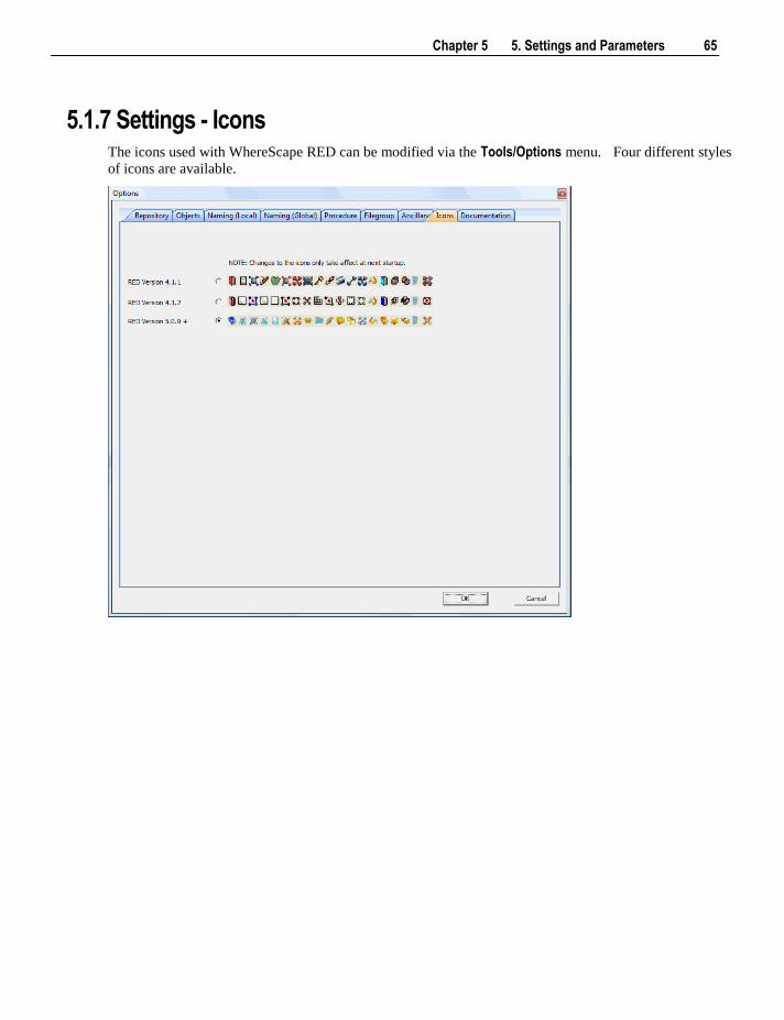
Chapter 5 5. Settings and Parameters 65
5.1.7 Settings - Icons The icons used with WhereScape RED can be modified via the Tools/Options menu. Four different styles
of icons are available.
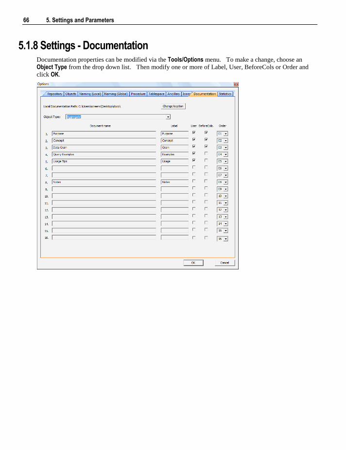
66 5. Settings and Parameters
5.1.8 Settings - Documentation Documentation properties can be modified via the Tools/Options menu. To make a change, choose an
Object Type from the drop down list. Then modify one or more of Label, User, BeforeCols or Order and
click OK.
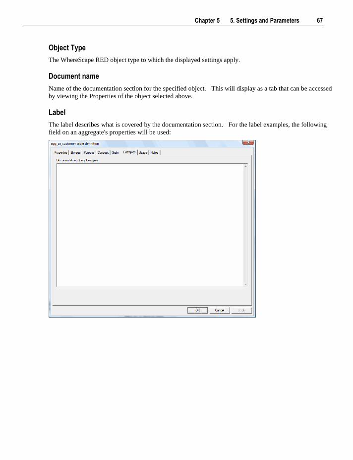
Chapter 5 5. Settings and Parameters 67
Object Type
The WhereScape RED object type to which the displayed settings apply.
Document name
Name of the documentation section for the specified object. This will display as a tab that can be accessed
by viewing the Properties of the object selected above.
Label
The label describes what is covered by the documentation section. For the label examples, the following
field on an aggregate's properties will be used:
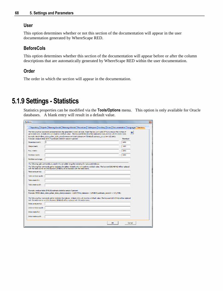
68 5. Settings and Parameters
User
This option determines whether or not this section of the documentation will appear in the user
documentation generated by WhereScape RED.
BeforeCols
This option determines whether this section of the documentation will appear before or after the column
descriptions that are automatically generated by WhereScape RED within the user documentation.
Order
The order in which the section will appear in the documentation.
5.1.9 Settings - Statistics Statistics properties can be modified via the Tools/Options menu. This option is only available for Oracle
databases. A blank entry will result in a default value.
Chapter 5 5. Settings and Parameters 69
Note: The example commands below contain returns and indents, these should be removed when entering
into the fields in this options screen.
Procedure Statistic Command Call Example
BEGIN
dbms_stats.gather_table_stats(ownname=>USER,tabname=>'$TABLE$'
,estimate_percent=>10);
END;
Threshold
The threshold parameter is used by the four statistic commands that are inserted into the automatically
generated procedures. It indicates how many rows to be inserted before the statistic commands are
executed.
Dimension insert
Statistics command entered here will be included in the automatically generated procedure for Dimension
tables. Parameter $TABLE$ will be automatically replaced by the table name. The key word
$UNUSED$ will remove the statistics portion from the generated code in procedure.
Stage insert
Statistics command entered here will be included in the automatically generated procedure for Stage tables.
Parameter $TABLE$ will be automatically replaced by the table name. The key word $UNUSED$ will
remove the statistics portion from the generated code in procedure.
Fact insert
Statistics command entered here will be included in the automatically generated procedure for Fact tables.
Parameter $TABLE$ will be automatically replaced by the table name. The key word $UNUSED$ will
remove the statistics portion from the generated code in procedure.
Partition insert
Statistics command entered here will be included in the automatically generated procedure for Partition
tables. Parameter $TABLE$ will be automatically replaced by the table name. The key word
$UNUSED$ will remove the statistics portion from the generated code in procedure.
Partition exchange
Statistics command entered here will be included in the automatically generated procedure during partition
exchanges. Parameter $TABLE$ will be automatically replaced by the table name. The key word
$UNUSED$ will remove the statistics portion from the generated code in procedure.
Scheduler Table Statistic Command Call Example
Analyze
analyze table $TABLE$ estimate statistics sample 35 percent
70 5. Settings and Parameters
Stats
BEGIN
dbms_stats.gather_table_stats(ownname=>'$SCHEMA$',,tabname=>'$TABLE$'
,estimate_percent=>'10');
END;
Table analyze full
Analyze command entered here will be executed when using the scheduler with Analyze Action to gather
statistics. Parameter $TABLE$ will be automatically replaced by the table name.
Table analyze quick
Analyze command entered here will be executed when using the scheduler with Quick Analyze Action to
gather statistics. Parameter $TABLE$ will be automatically replaced by the table name.
Table stats full
Statistics command entered here will be executed when using the scheduler with Stats Action to gather
statistics. Parameter $TABLE$ will be automatically replaced by the table name and parameter
$SCHEMA$ will be replaced by the owner name.
Table stats quick
Statistics command entered here will be executed when using the scheduler with Quick Stats Action to
gather statistics. Parameter $TABLE$ will be automatically replaced by the table name and parameter
$SCHEMA$ will be replaced by the owner name.
Scheduler Index Statistic Command Call Example
Analyze
analyze index $INDEX$ estimate statistics sample 5 percent
Stats
BEGIN
dbms_stats.gather_index_stats(ownname=>'$SCHEMA$',,indname=>'$INDEX$'
,estimate_percent=>'10');
END;
Index analyze full
Analyze command entered here will be executed when using the scheduler with Analyze Action to gather
statistics. Parameter $INDEX$ will be automatically replaced by the index name.
Index analyze quick
Analyze command entered here will be executed when using the scheduler with Quick Analyze Action to
gather statistics. Parameter $INDEX$ will be automatically replaced by the index name.
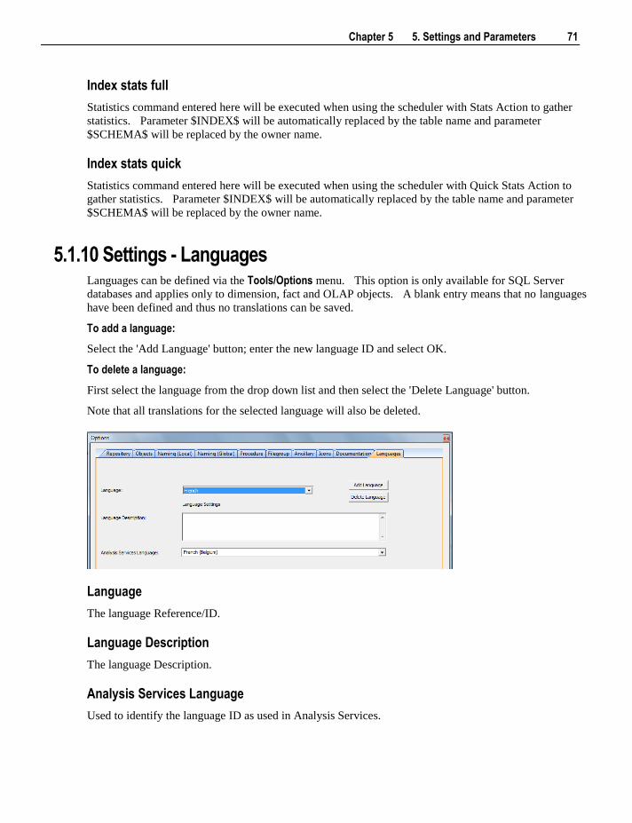
Chapter 5 5. Settings and Parameters 71
Index stats full
Statistics command entered here will be executed when using the scheduler with Stats Action to gather
statistics. Parameter $INDEX$ will be automatically replaced by the table name and parameter
$SCHEMA$ will be replaced by the owner name.
Index stats quick
Statistics command entered here will be executed when using the scheduler with Quick Stats Action to
gather statistics. Parameter $INDEX$ will be automatically replaced by the table name and parameter
$SCHEMA$ will be replaced by the owner name.
5.1.10 Settings - Languages Languages can be defined via the Tools/Options menu. This option is only available for SQL Server
databases and applies only to dimension, fact and OLAP objects. A blank entry means that no languages
have been defined and thus no translations can be saved.
To add a language:
Select the 'Add Language' button; enter the new language ID and select OK.
To delete a language:
First select the language from the drop down list and then select the 'Delete Language' button.
Note that all translations for the selected language will also be deleted.
Language
The language Reference/ID.
Language Description
The language Description.
Analysis Services Language
Used to identify the language ID as used in Analysis Services.
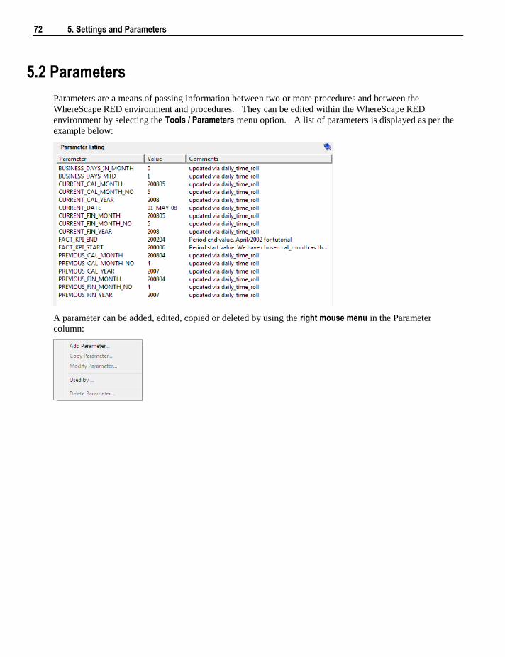
72 5. Settings and Parameters
5.2 Parameters
Parameters are a means of passing information between two or more procedures and between the
WhereScape RED environment and procedures. They can be edited within the WhereScape RED
environment by selecting the Tools / Parameters menu option. A list of parameters is displayed as per the
example below:
A parameter can be added, edited, copied or deleted by using the right mouse menu in the Parameter
column:
Chapter 5 5. Settings and Parameters 73
Typical parameter usage may be the global definition of how many days should be looked back for changed
data, a month or processing period etc.
Parameters can be used in load tables to place limits in a Where clause, etc. See Database Link Load -
Source Mapping (see "8.3.2 Database Link Load - Source Mapping" on page 125) for more information.
They are also used by stage table procedures as variables. See Generating the Staging Update Procedure
(see "11.3 Generating the Data Store Update Procedure" on page 224) for more information.
IBM DB2: Two procedures are provided to allow procedures to read and write parameters. These
procedures are WsParameterRead (see "29.20 WsParameterRead" on page 644) and WsParameterWrite
(see "29.23 WsParameterWrite" on page 653). Using these procedures a procedure can load and use the
contents of a parameter, or modify an existing parameter, or add a new parameter.
Oracle: Two functions are provided to allow procedures to read and write parameters. These functions are
WsParameterRead (see "29.20 WsParameterRead" on page 644) and WsParameterWrite (see "29.23
WsParameterWrite" on page 653). Using these functions a procedure can load and use the contents of a
parameter, or modify an existing parameter, or add a new parameter.
SQL Server: Two procedures are provided to allow procedures to read and write parameters. These
procedures are WsParameterRead (see "29.20 WsParameterRead" on page 644) and WsParameterWrite
(see "29.23 WsParameterWrite" on page 653). Using these procedures a procedure can load and use the
contents of a parameter, or modify an existing parameter, or add a new parameter. A function
WsParameterReadF (see "29.20 WsParameterRead" on page 644) is also provided. This function will
return the value of a parameter.
Global Parameters
A number of global parameters are provided when loading tables either via WhereScape RED or via the
scheduler. These global parameters are accessed by calling the function WsParameterReadG (see "29.21
WsParameterReadG" on page 647). The load table name and the source table name can be acquired by
using this function.
See Callable Procedures (see "29. Callable Procedures" on page 565) for more information on
WsParameterRead (see "29.20 WsParameterRead" on page 644), WsParameterWrite (see "29.23
WsParameterWrite" on page 653), WsParameterReadF (see "29.20 WsParameterRead" on page 644) and
WsParameterReadG (see "29.21 WsParameterReadG" on page 647).

Chapter 6 6. Connections 75
In This Chapter
6.1 Connections Overview .......................................................... 75
6.2 Connection to the Data Warehouse ....................................... 78
6.3 Connections to Another Database ......................................... 84
6.4 ODBC Based Connections .................................................... 93
6.5 Connections to Unix ............................................................. 95
6.6 Connections to Windows ...................................................... 99
6.7 Connections to Analysis Services ......................................... 103
6.1 Connections Overview
Connection objects serve several purposes in WhereScape RED:
1 They are used to browse potential source data in source systems and to acquire metadata. Potential
source data includes database tables and flat files. For database tables, WhereScape RED:
Uses the ODBC Source set on each connection to browse the source system.
Acquires the metadata for new load tables built from the source system using drag and drop.
For flat files, WhereScape RED:
Connects directly to Windows, Linux or Unix to analyze the source file for the new load table and
acquire its metadata.
Prompts for user input for any metadata not available in the source file.
Note: Windows and Unix connections do not have an ODBC Source property. Unix connections are
used for Unix and Linux systems.
2 Load tables with a connection of Connection type ODBC extract data from source systems using
ODBC. The ODBC Source of the connection is the ODBC DSN used for the extract.
3 Each data warehouse metadata repository must have a Data Warehouse connection to use drag and
drop to create new objects (other than load tables) in the data warehouse. WhereScape RED:
Uses the ODBC Source set on the Data Warehouse connection to browse the Data Warehouse
database.
Acquires the metadata for any tables built from existing data warehouse tables.
Note: This connection always has a Connection type of Database.
4 Cube objects require a connection to define the Analysis Services server used to create and load cubes.
This is a connection with a Connection type of Analysis Server 2000 if SQL Server 2000 OLAP is being
used. The Connection type is Microsoft Analysis Server 2005 for later versions of SQL Server OLAP.
C H A P T E R 6
6. Connections

76 6. Connections
5 Export objects require a connection to define the target environment where exported data is written.
This is a connection with a Connection type of Unix or Windows.
The tables or files associated with a connection are displayed one of the following ways:
Selecting the Browse / Data warehouse menu option nominally for the data warehouse connection.
Selecting the Browse / Source Tables menu option nominally for a source system connection.
Clicking on one of the two browser buttons on the toolbar:
The orange button is nominally for the data warehouse connection and the blue button is nominally for
a source system connection.
Clicking on one of the browse source system buttons in the right pane:
Each button remembers the last connection it browsed, so in this way one button can be used for the Data
Warehouse and one for a source system. A click on one of the buttons will display the source tables
without first displaying the source browser dialog box. To change the connection click the small black
down arrow next to the glasses to access the source browser dialog box. The current connection being
browsed is shown in the status bar at the bottom right of the screen.
TIP: When browsing to a connection, by default WhereScape RED will show a schema name. If
you want to see all schemas, blank out the default schema name. You can also enter multiple schemas,
separated by commas.
Browser Icons
When browsing a connection the following legend applies for the source tables and objects:
Chapter 6 6. Connections 77
The legend is displayed via Help / Source Legend menu.
Connection types
Connections can be set up via the following methods:
Connection to the Data Warehouse (see "6.2 Connection to the Data Warehouse" on page 78)
Connections to Another Database (see "6.3 Connections to Another Database" on page 84)
ODBC Based Connections (see "6.4 ODBC Based Connections" on page 93)
Connections to Unix (see "6.5 Connections to Unix" on page 95)
Connections to Windows (see "6.6 Connections to Windows" on page 99)
Connections to Analysis Services (see "6.7 Connections to Analysis Services" on page 103)
78 6. Connections
6.2 Connection to the Data Warehouse
This section describes the connection to the Data Warehouse. Tutorial 1 gives basic instructions for
creating a connection. This topic describes in greater detail the connection properties as they apply to the
Data Warehouse connection. This connection is used in the drag and drop functionality to create the
dimension, stage, fact and aggregate tables. It is also used to create cubes.
TIP: The Data Warehouse connection must exist if you wish to use drag and drop to create
dimensions, stage tables, fact tables, aggregates and cubes.
Datawarehouse check box
There should only be one data warehouse connection in any WhereScape RED repository. The data
warehouse connection must have the Datawarehouse check box enabled. No other connection should have
this check box enabled.
Connection name
Enter a name for the connection. Typically this is 'Data warehouse'
Connection type
The connection type is Database.
ODBC Source
The ODBC Source is the name as defined in the Windows 'ODBC Data Source Administrator'. This
Administrator is found in the Control Panel of the PC. The ODBC Source must be a valid User or System
DSN and for Oracle must have the 'Server' field set to the Tnsnames entry for the data warehouse database.
Provider Name
Leave Blank
TIP: For Oracle the ODBC driver used for the ODBC Source must be the Microsoft ODBC Driver
for Oracle Version 2.573.6019.00 or later.
If multiple PCs are accessing the meta repository there needs to be a standard naming convention such that
all PCs use the same ODBC Source name.
TIP: The same ODBC source name must be used on all PCs that use this connection.
Oracle Example Screen:
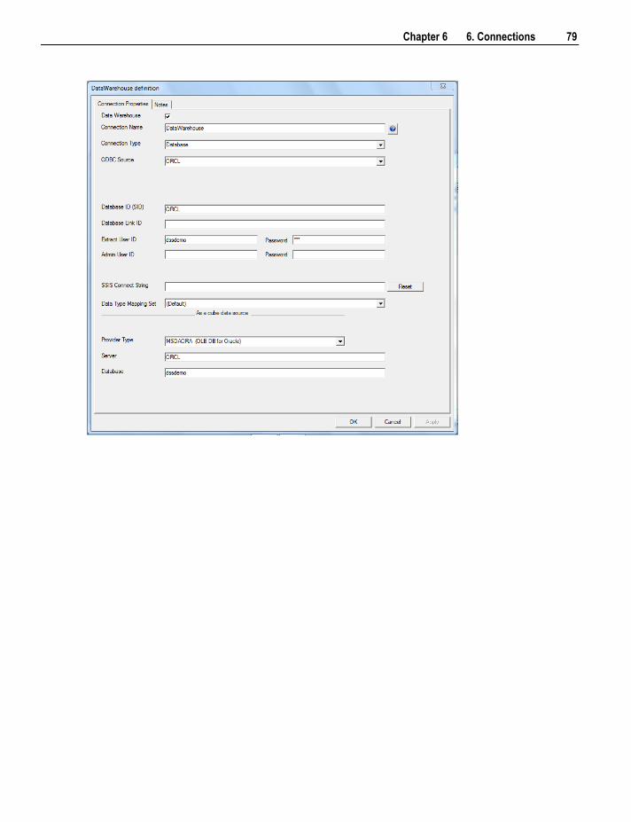
Chapter 6 6. Connections 79
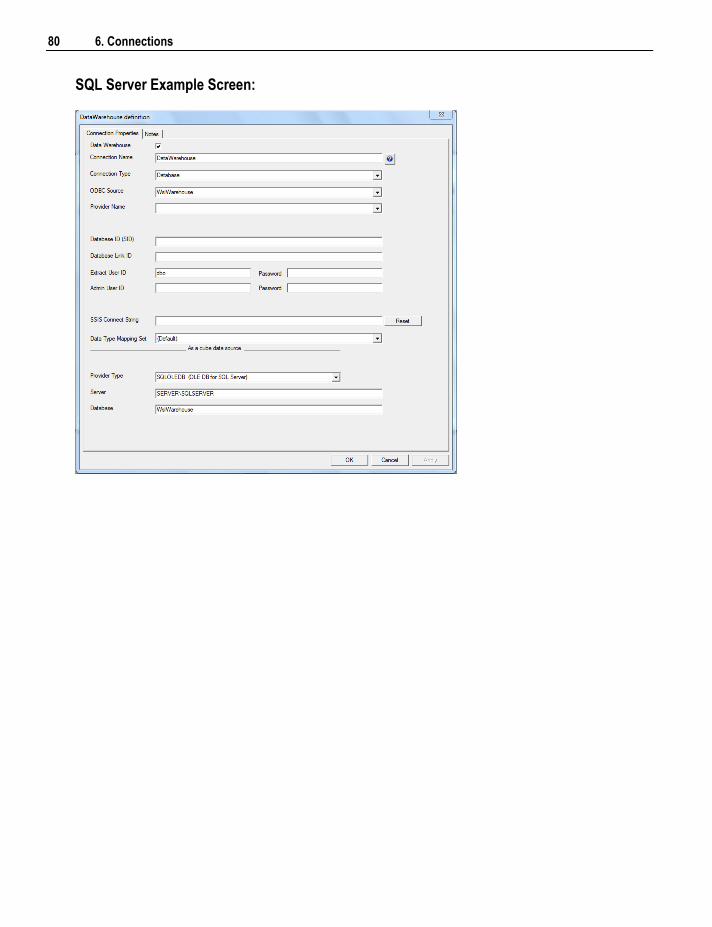
80 6. Connections
SQL Server Example Screen:
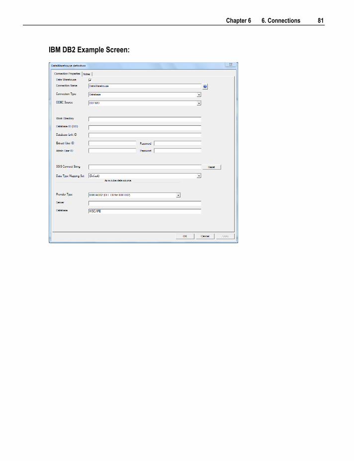
Chapter 6 6. Connections 81
IBM DB2 Example Screen:
82 6. Connections
Work Directory
The work directory must be an existing valid Windows directory.
Database id (SID)
For SQL Server and DB2 leave this field blank. For Oracle enter the database id of the Data Warehouse
database, e.g, ORCL.
Database link id
As this is a link back to the data warehouse this field must be left blank.
Extract user id
Enter the data warehouse user id. That is the database username under which the meta repository is loaded.
For SQL Server this must be dbo if a trusted connection or the server login id. For DB2, this should be left
blank if OS authentication is being used.
Extract password
The password of the data warehouse user. For SQL Server blank if a trusted login, or the server login
password. For DB2, this should be left blank if OS authentication is being used.
Admin user id
Left blank.
Admin password
Left blank.
For cubes, the properties dialog shows some additional columns at the bottom of the screen. These are
required so that the data warehouse can be used as a source for the Analysis Services cubes. Some other
fields are determined by the type of relation database being used for the data warehouse. These fields are:
SSIS Connect String
SSIS Connect String is a valid SSIS connection string that can be used to connect to the data source or
destination. The Reset button will attempt to construct a valid connection string from the connection
information supplied in the connection details consisting of the Database ID, Database Link ID (Instance
name), Provider Name, Extract User details.
Data Type Mapping Set
XML files have been created to store mappings from one set of data types to another. Setting this field to
"(Default)" will cause RED to automatically select the relevant mapping set; otherwise you can choose one
of the standard mapping sets from the drop down list or create a new one.
As a cube data source:
This section of fields is only relevant and will only be visible if the Datawarehouse check box has been
enabled.
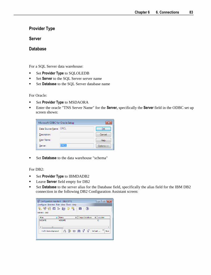
Chapter 6 6. Connections 83
Provider Type
Server
Database
For a SQL Server data warehouse:
Set Provider Type to SQLOLEDB
Set Server to the SQL Server server name
Set Database to the SQL Server database name
For Oracle:
Set Provider Type to MSDAORA
Enter the oracle "TNS Server Name" for the Server, specifically the Server field in the ODBC set up
screen shown:
Set Database to the data warehouse "schema"
For DB2:
Set Provider Type to IBMDADB2
Leave Server field empty for DB2
Set Database to the server alias for the Database field, specifically the alias field for the IBM DB2
connection in the following DB2 Configuration Assistant screen:
84 6. Connections
6.3 Connections to Another Database
This section describes connections to another database source where a database link can be established.
If running a SQL Server data warehouse it is possible to create database links (linked server) to other SQL
Server instances and most of the other major databases such as Oracle, DB2 etc.
Using the Oracle database it is possible to create a database link to another Oracle database as standard, or
to any other database by using Oracles Heterogeneous Services. Tutorial 1 gives basic instructions for
creating a connection. This topic describes in greater detail the connection properties. From this type of
connection you can do database link loads.
When coming to the Data Warehouse from an OLTP source system, the connection defines the path to get
to those source tables. A connection object must be defined for each source system.
The connection object properties window has the following fields:
Connection name
Enter a name for the connection. Typically this is a name that identifies the source system.
Connection type
The connection type is Database.
ODBC Source
The ODBC Source is the name as defined in the Windows 'ODBC Data Source Administrator'. This
Administrator is found in the Control Panel of the PC. The ODBC Source must be a valid User or System
DSN. For Oracle sources the 'Server' field must be set to the Tnsnames entry for the source system
database.
TIP: For Oracle sources the ODBC driver used for the ODBC Source must be the Microsoft ODBC
Driver for Oracle Version 2.573.6019.00 or later. If the source database is SQL Server, Progress,
Informix, DB2, Sybase, Ingres or some other database then the ODBC driver available can be tested or you
can contact WhereScape for a list of proven drivers.
If multiple PCs are accessing the meta repository there needs to be a standard naming convention such that
all PCs use the same ODBC Source name.
TIP: The same ODBC source name must be used on all PCs that use this connection.
Provider Name
For SQL Server this is the name of the server or a provider type selected from the drop down list. To
connect to another SQL Server database that resides on a different server select SQLOLEDB. In the
example below MSDAORA is chosen for a connection to an oracle database.
Database id (SID)
For Oracle enter the database id of the Source database. For SQL Server enter the database name.
Chapter 6 6. Connections 85
Database link id
If a database link already exists to this source database then enter that link name in this field. If no link
exists then enter a link name. Under some circumstances Oracle insists that this link name is the same as
the tnsnames entry for the database, so it may be good practice to use the source SID as the database link
name. If this is a new link then see the notes later in this section on database link creation (see "6.3.1
Database Link Creation" on page 91).
If SQL Server and the database are on the same server as the data warehouse then no link needs to be
defined, so this field can be left blank. Enter the defined SQL LINK name that points to the correct server,
the link name does not need to be the same name as the server name.
If Oracle and the source tables are in the same database then no link is required and this field must be left
blank.
Extract user id
Enter the source system user id under which you can logon to the source system. This is not necessarily
the user that owns the tables you will be extracting. It must, however, be a user that has 'Select' access to
the tables you wish to extract. For more information see remote view extract (see "8.3.3 Remote View
Extract" on page 129).
Extract password
The password of the user on the source system
Admin user id
Leave blank.
Admin password
Leave blank.
SSIS Connect String
SSIS Connect String is a valid SSIS connection string that can be used to connect to the data source or
destination. The Reset button will attempt to construct a valid connection string from the connection
information supplied in the connection details consisting of the Database ID, Database Link ID (Instance
name), Provider Name, Extract User details.
Data Type Mapping Set
XML files have been created to store mappings from one set of data types to another. Setting this field to
"(Default)" will cause RED to automatically select the relevant mapping set; otherwise you can choose one
of the standard mapping sets from the drop down list or create a new one.
Once the connection has been set up, you can right mouse click the connection in the middle pane and view
the properties for that connection.
Browsing a connection
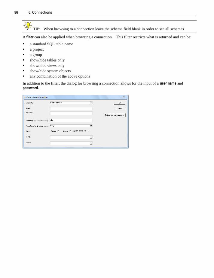
86 6. Connections
TIP: When browsing to a connection leave the schema field blank in order to see all schemas.
A filter can also be applied when browsing a connection. This filter restricts what is returned and can be:
a standard SQL table name
a project
a group
show/hide tables only
show/hide views only
show/hide system objects
any combination of the above options
In addition to the filter, the dialog for browsing a connection allows for the input of a user name and password.
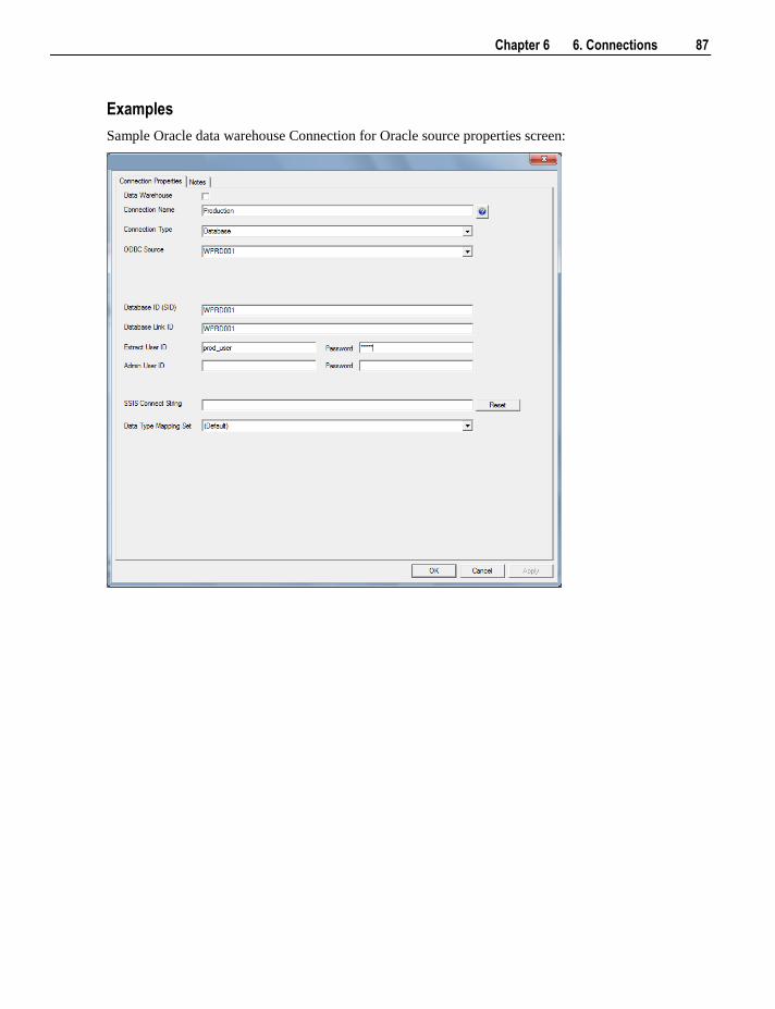
Chapter 6 6. Connections 87
Examples
Sample Oracle data warehouse Connection for Oracle source properties screen:
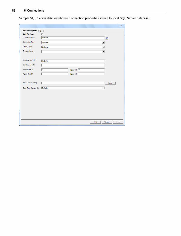
88 6. Connections
Sample SQL Server data warehouse Connection properties screen to local SQL Server database:
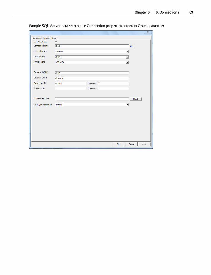
Chapter 6 6. Connections 89
Sample SQL Server data warehouse Connection properties screen to Oracle database:
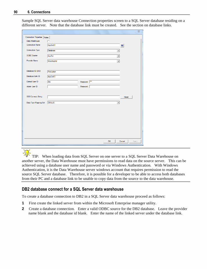
90 6. Connections
Sample SQL Server data warehouse Connection properties screen to a SQL Server database residing on a
different server. Note that the database link must be created. See the section on database links.
TIP: When loading data from SQL Server on one server to a SQL Server Data Warehouse on
another server, the Data Warehouse must have permissions to read data on the source server. This can be
achieved using a database user name and password or via Windows Authentication. With Windows
Authentication, it is the Data Warehouse server windows account that requires permission to read the
source SQL Server database. Therefore, it is possible for a developer to be able to access both databases
from their PC and a database link to be unable to copy data from the source to the data warehouse.
DB2 database connect for a SQL Server data warehouse
To create a database connection to DB2 in a SQL Server data warehouse proceed as follows:
1 First create the linked server from within the Microsoft Enterprise manager utility.
2 Create a database connection. Enter a valid ODBC source for the DB2 database. Leave the provider
name blank and the database id blank. Enter the name of the linked server under the database link.
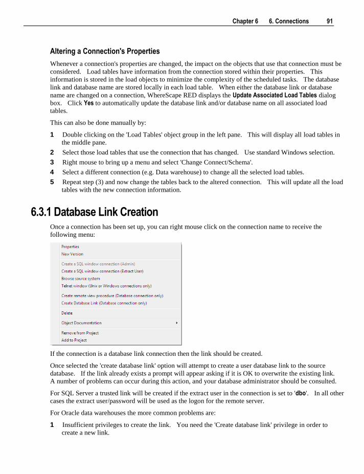
Chapter 6 6. Connections 91
Altering a Connection's Properties
Whenever a connection's properties are changed, the impact on the objects that use that connection must be
considered. Load tables have information from the connection stored within their properties. This
information is stored in the load objects to minimize the complexity of the scheduled tasks. The database
link and database name are stored locally in each load table. When either the database link or database
name are changed on a connection, WhereScape RED displays the Update Associated Load Tables dialog
box. Click Yes to automatically update the database link and/or database name on all associated load
tables.
This can also be done manually by:
1 Double clicking on the 'Load Tables' object group in the left pane. This will display all load tables in
the middle pane.
2 Select those load tables that use the connection that has changed. Use standard Windows selection.
3 Right mouse to bring up a menu and select 'Change Connect/Schema'.
4 Select a different connection (e.g. Data warehouse) to change all the selected load tables.
5 Repeat step (3) and now change the tables back to the altered connection. This will update all the load
tables with the new connection information.
6.3.1 Database Link Creation Once a connection has been set up, you can right mouse click on the connection name to receive the
following menu:
If the connection is a database link connection then the link should be created.
Once selected the 'create database link' option will attempt to create a user database link to the source
database. If the link already exists a prompt will appear asking if it is OK to overwrite the existing link.
A number of problems can occur during this action, and your database administrator should be consulted.
For SQL Server a trusted link will be created if the extract user in the connection is set to 'dbo'. In all other
cases the extract user/password will be used as the logon for the remote server.
For Oracle data warehouses the more common problems are:
1 Insufficient privileges to create the link. You need the 'Create database link' privilege in order to
create a new link.
92 6. Connections
2 TNS could not resolve the connection to the remote database. The database link uses the value entered
in the 'SID' field of the connection to identify the remote database. This value must be a valid entry in
the Tnsnames table for the source database.
Chapter 6 6. Connections 93
6.4 ODBC Based Connections
This connection is via an ODBC link. All data movement is performed using the ODBC connection.
Connection name
A name to define your connection.
Connection type
ODBC.
ODBC Source
The ODBC Source is the name as defined in the Windows 'ODBC Data Source Administrator'. This
Administrator is found in the Control Panel of the PC. The ODBC Source must be a valid User or System
DSN and for Oracle sources must have the 'Server' field set to the Tnsnames entry for the data warehouse
database.
TIP: For Oracle data source the ODBC driver used for the ODBC Source must be the Microsoft
ODBC Driver for Oracle Version 2.573.6019.00 or later.
If multiple PCs are accessing the meta repository there needs to be a standard naming convention such that
all PCs use the same ODBC Source name.
TIP: The same ODBC source name must be used on all PCs that use this connection.
Work directory
The work directory must be an existing valid Windows directory.
TIP: This directory must be valid on the Server that is running the Scheduler.
Extract user id
Enter the source system user id under which you can logon to the source system. This is not necessarily
the user that owns the tables you will be extracting. It must, however, be a user that has 'Select' access to
the tables you wish to extract.
Extract password
The password of the user on the source system
Admin user id
Leave blank.
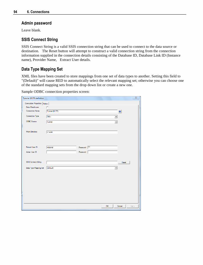
94 6. Connections
Admin password
Leave blank.
SSIS Connect String
SSIS Connect String is a valid SSIS connection string that can be used to connect to the data source or
destination. The Reset button will attempt to construct a valid connection string from the connection
information supplied in the connection details consisting of the Database ID, Database Link ID (Instance
name), Provider Name, Extract User details.
Data Type Mapping Set
XML files have been created to store mappings from one set of data types to another. Setting this field to
"(Default)" will cause RED to automatically select the relevant mapping set; otherwise you can choose one
of the standard mapping sets from the drop down list or create a new one.
Sample ODBC connection properties screen:
Chapter 6 6. Connections 95
6.5 Connections to Unix
Note: Unix connections are only supported from Oracle and DB2 data warehouses.
This section describes connections to Unix. Tutorial 1 gives basic instructions for creating a connection.
This topic describes in greater detail the connection properties as they apply to Unix connections.
From a Unix connection you can only do flat file loads.
TIP: If the connection type is Linux then the connection name must contain the word Linux. This
forces WhereScape RED to use /bin/sh shell instead of /bin/ksh shell.
Connection name
Enter a name for the connection. See the above tip regarding Linux connections.
Connection type
The connection type is Unix. See the above tip regarding Linux connections.
Host name
Enter the IP address or the host name of the Unix host.
Work directory
The directory must be a valid directory that you have write access to on the Unix machine, typically /tmp. This directory must be unique if multiple schedulers are running on the same Unix machine.
Note: There must be a different work directory for each scheduler running on a Unix platform. If this is not
done and common usernames/passwords are used then the possibility exists that the wrong script or file
based load could be processed.
Database id (SID)
Enter the database id of the Data Warehouse database, e.g, ORCL
Database home directory
If the home directory is different from the standard Oracle home directory then enter the directory here.
Unix user id
Enter the name of the Unix user being logged on to. That user must log on to the shell prompt for drag and
drop features to be used.
Unix password
The password of the Unix user being logged on to.
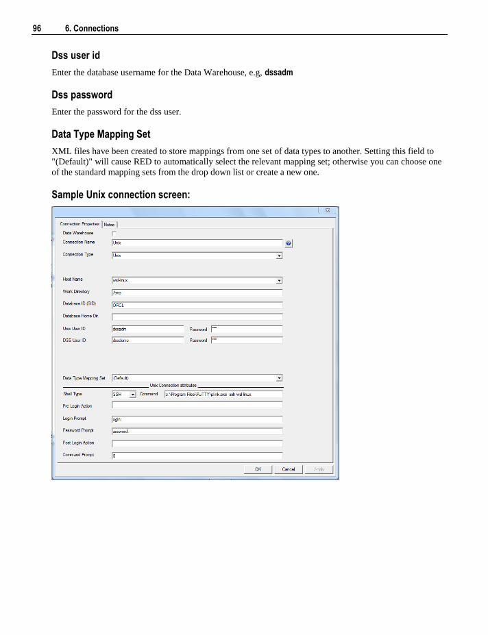
96 6. Connections
Dss user id
Enter the database username for the Data Warehouse, e.g, dssadm
Dss password
Enter the password for the dss user.
Data Type Mapping Set
XML files have been created to store mappings from one set of data types to another. Setting this field to
"(Default)" will cause RED to automatically select the relevant mapping set; otherwise you can choose one
of the standard mapping sets from the drop down list or create a new one.
Sample Unix connection screen:
Chapter 6 6. Connections 97
Shell Type
The shell type is either Telnet or SSH (secure shell). If SSH is selected, then the Command box is made
available.
Command
This is the command used by SSH for securing a connection to the LINUX or UNIX server.
Pre Login Action, Login prompt, Password prompt, Post login action, and Command prompt.
These fields are only used to create a Telnet connection to the host machine. WhereScape RED uses the
Telnet connection in the drag and drop functionality. It is not used in the actual production running of the Data Warehouse, and is only necessary if you wish to use the drag and drop functionality.
Pre Login Action
Only used as above, e.g, /n (to initiate a carriage return before the prompt).
Login prompt
The Unix login prompt, or the tail end of the login prompt, e.g, ogin:
Password prompt
The Unix password prompt, or the tail end of the password prompt, e.g, assword:
Post login action
Not often used but may be necessary to respond to a login question. It is preferable that the Unix login
goes straight to the command prompt.
Command prompt
Enter the Unix command prompt, or the tail end of that prompt, typically $
Note: In order to ascertain some of the above fields you will have to log in to the Unix system.
To validate the fields
Right click on the connection name
Select Telnet window
This will provide a telnet window that can be used to log on to the Unix server.
To test the drag and drop functionality
From the menu strip select Browse | Source Tables
Drill down to the area required
Drag an item to the middle pane, (having first selected the object in the left pane).
Connection Failures
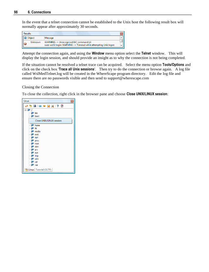
98 6. Connections
In the event that a telnet connection cannot be established to the Unix host the following result box will
normally appear after approximately 30 seconds.
Attempt the connection again, and using the Window menu option select the Telnet window. This will
display the login session, and should provide an insight as to why the connection is not being completed.
If the situation cannot be resolved a telnet trace can be acquired. Select the menu option Tools/Options and
click on the check box 'Trace all Unix sessions'. Then try to do the connection or browse again. A log file
called WslMedTelnet.log will be created in the WhereScape program directory. Edit the log file and
ensure there are no passwords visible and then send to [email protected]
Closing the Connection
To close the collection, right click in the browser pane and choose Close UNIX/LINUX session:
Chapter 6 6. Connections 99
6.6 Connections to Windows
This connection is back to the PC that you are working on, or to a host Windows PC. From Windows you
can only do flat file loads.
Connection name
A name to define your connection.
Connection type
Windows.
Host name
Leave this blank if you are connecting to your own PC. If you are connecting remotely to another
Windows system, enter the name of that system.
Work directory
The work directory must be an existing valid Windows directory.
TIP: If a Windows Scheduler is being used then this directory must be valid on the Server that is
running the Scheduler.
Database id (SID)
Enter the database id for the Data Warehouse database.
Database home directory
Enter the directory name here only if it differs from the standard.
Windows user id and password
Leave this blank if you are connecting to your own PC. Enter details if you are connecting remotely to
another Windows system.
Dss user id and password
Enter the relevant details for connecting to the Data Warehouse.
Data Type Mapping Set
XML files have been created to store mappings from one set of data types to another. Setting this field to
"(Default)" will cause RED to automatically select the relevant mapping set; otherwise you can choose one
of the standard mapping sets from the drop down list or create a new one.
To test the connection
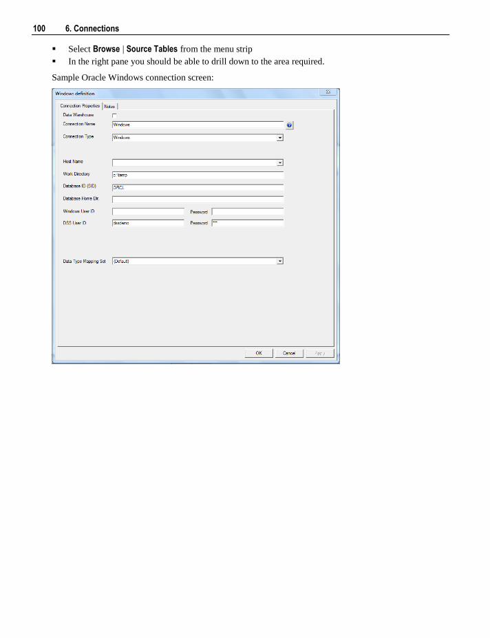
100 6. Connections
Select Browse | Source Tables from the menu strip
In the right pane you should be able to drill down to the area required.
Sample Oracle Windows connection screen:
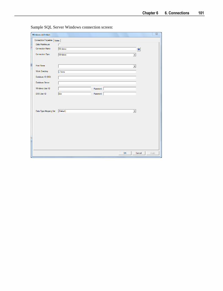
Chapter 6 6. Connections 101
Sample SQL Server Windows connection screen:
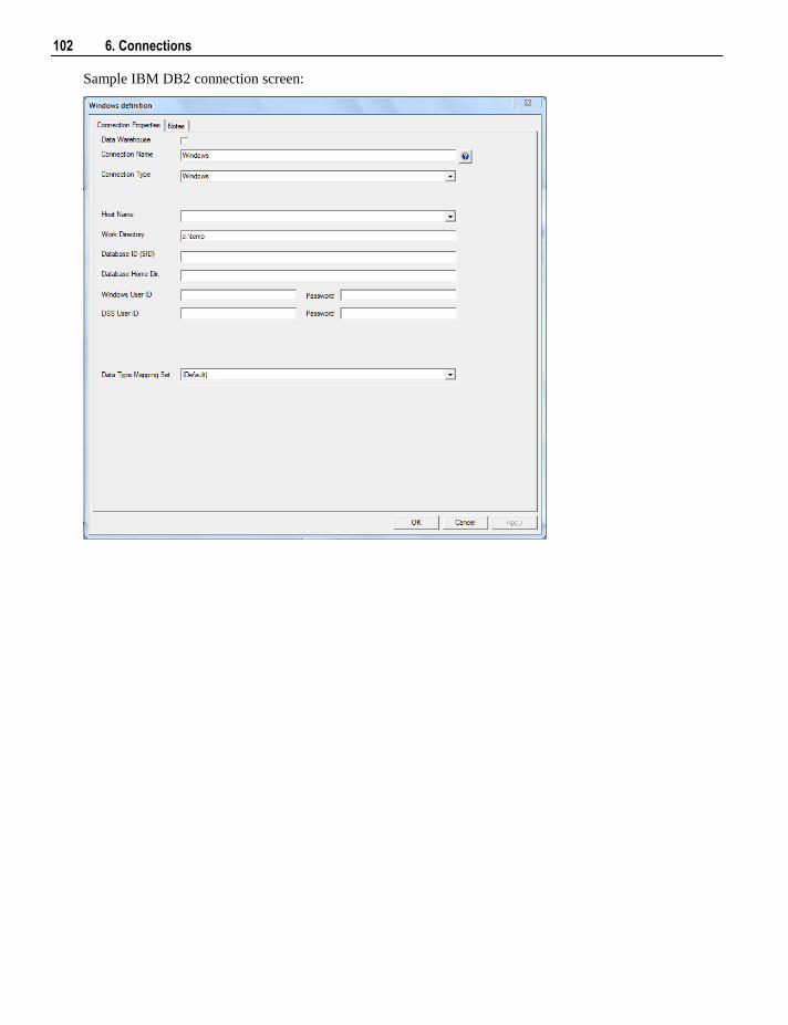
102 6. Connections
Sample IBM DB2 connection screen:
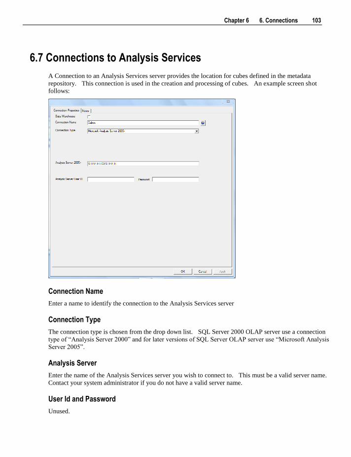
Chapter 6 6. Connections 103
6.7 Connections to Analysis Services
A Connection to an Analysis Services server provides the location for cubes defined in the metadata
repository. This connection is used in the creation and processing of cubes. An example screen shot
follows:
Connection Name
Enter a name to identify the connection to the Analysis Services server
Connection Type
The connection type is chosen from the drop down list. SQL Server 2000 OLAP server use a connection
type of “Analysis Server 2000” and for later versions of SQL Server OLAP server use “Microsoft Analysis
Server 2005”.
Analysis Server
Enter the name of the Analysis Services server you wish to connect to. This must be a valid server name.
Contact your system administrator if you do not have a valid server name.
User Id and Password
Unused.

Chapter 7 7. Table Properties 105
Several generic properties can be set on all table objects in WhereScape RED. These are:
Storage Properties
Notes
Documentation Fields
This Chapter discusses these properties.
In This Chapter
7.1 Table Storage Properties ....................................................... 106
7.2 Table Notes ........................................................................... 111
7.3 Table Documentation Fields ................................................. 113
7.4 Table Statistics in DB2 ......................................................... 114
C H A P T E R 7
7. Table Properties
106 7. Table Properties
7.1 Table Storage Properties
The fields on the Storage tab of the Properties screen for tables are described below. The properties
available depend on the data warehouse database environment.
For a SQL Server example, see Table Storage Screen - SQL Server (see "7.1.1 Table Storage Screen -
SQL Server" on page 108).
For an Oracle example, see Table Storage Screen - Oracle (see "7.1.2 Table Storage Screen - Oracle"
on page 109).
For a DB2 example, see Table Storage Screen - DB2 (see "7.1.3 Table Storage Screen - DB2" on page
111).
Tablespace / Filegroup name
Select a name from the drop down list box. If no tablespace is selected in Oracle or DB2, then the default
tablespace for the schema is used. If no filegroup name is selected for SQL Server, the default for the
database is used.
VarDecimal
Enables variable numeric storage in SQL Server for the table. The default is off - no variable numeric
storage. To enable variable number storage, the following command must also be run for the SQL Server
database: sp_db_vardecimal_storage_format 'DatabaseName', 'ON'
Initial extent (KB)
Oracle only. The size of the first extent of a created database table. The default is 0 kilobytes - use the
tablespace's default value. For locally managed tablespaces, this field is ignored.
Next extent (KB)
Oracle only. The size of the next (second) extent of a created database table, unless percent increase is
specified. The default is 0 kilobytes - use the tablespace's default value. For locally managed tablespaces,
this field is ignored.
Minimum extents
Oracle only. The number of extents the table is created with. The default is 0 - use the tablespace's
default value. For locally managed tablespaces, this field is ignored.
Maximum extents
Oracle only. The maximum number of extents the table can have. The default is 0 - use the tablespace's
default value. For locally managed tablespaces, this field is ignored.
Percent increase
Oracle only. The size the next extent is as a percent of the previous extent added. For example, a value of
5 will create the next extent 5% bigger than the previous extent added. The default is 0 - use the
tablespace's default value. For locally managed tablespaces, this field is ignored.
Chapter 7 7. Table Properties 107
Percent free
Oracle and DB2 only. The amount of free space to leave in each extent in Oracle and each page in DB2.
The default is 0 - use the database default.
Buffer Pool attribute
Oracle Dimension tables only. Mark the table to be retained in a special buffer pool. Possible values are
Default, Keep, Recycle and not set (blank). The default is not set.
Compress
DB2 only. Enable table compression. Default is off - no compression.
Volatile
DB2 only. Enable this option to alter the table after it is created to indicate size volatility to the DB2
optimizer.
Append Only
DB2 only. Enable this option to alter the table after it is created to append new data to the end of the table,
rather than using available free space in the table.
Index build logging
DB2 only. Specifies the degree of logging performed by DB2 when creating, recreating and re-organizing
indexes. Value is one of not selected, NULL, OFF or ON. Not selected and NULL are the same. The table
is created without this option and then altered to add this property. The default is not set (no alter takes
place). The following describes the values:
NULL - Database parameter logindexbuild determines whether logging is minimal or full.
OFF - only minimal logging occurs.
ON - all operations are logged.
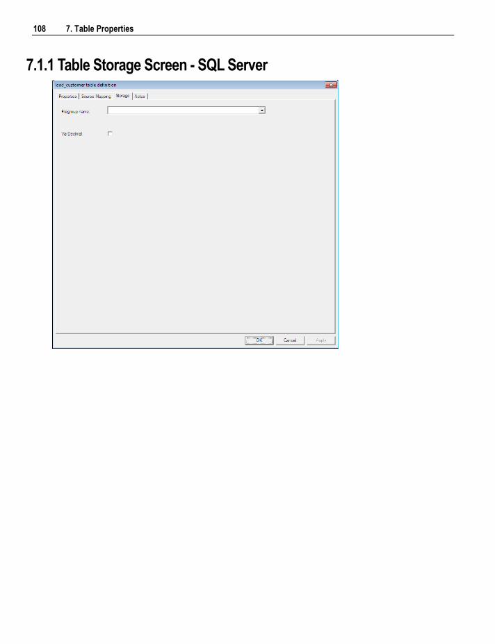
108 7. Table Properties
7.1.1 Table Storage Screen - SQL Server
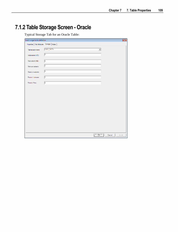
Chapter 7 7. Table Properties 109
7.1.2 Table Storage Screen - Oracle Typical Storage Tab for an Oracle Table:
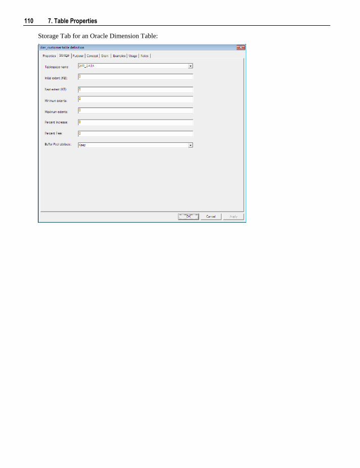
110 7. Table Properties
Storage Tab for an Oracle Dimension Table:
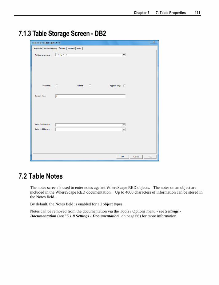
Chapter 7 7. Table Properties 111
7.1.3 Table Storage Screen - DB2
7.2 Table Notes
The notes screen is used to enter notes against WhereScape RED objects. The notes on an object are
included in the WhereScape RED documentation. Up to 4000 characters of information can be stored in
the Notes field.
By default, the Notes field is enabled for all object types.
Notes can be removed from the documentation via the Tools / Options menu - see Settings -
Documentation (see "5.1.8 Settings - Documentation" on page 66) for more information.
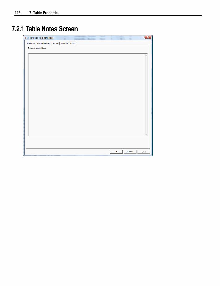
112 7. Table Properties
7.2.1 Table Notes Screen
Chapter 7 7. Table Properties 113
7.3 Table Documentation Fields
Each table has a set of associated documentation tabs. These are used to store descriptive metadata about
the fact table and how it is used. The contents of each tab appears in the generated documentation. Their
order and placement can be customized in the generated documentation using the Tools / Options menu.
The following tabs are available to store additional informational metadata that will appear in the generated
WhereScape RED documentation:
Purpose
Concept
Grain
Examples
Usage
Note: These names of the tabs are completely arbitrary and can be changed in the generated documentation
using Tools / Options menu, Documentation tab. By default, these fields are not enabled for load and stage
tables, but can be enabled using the Tools / Options menu, Documentation tab.
Up to 4000 characters of information can be stored in each field.
Some or all of these fields can be removed from the documentation via the Tools / Options menu - see
Settings - Documentation (see "5.1.8 Settings - Documentation" on page 66) for more information.
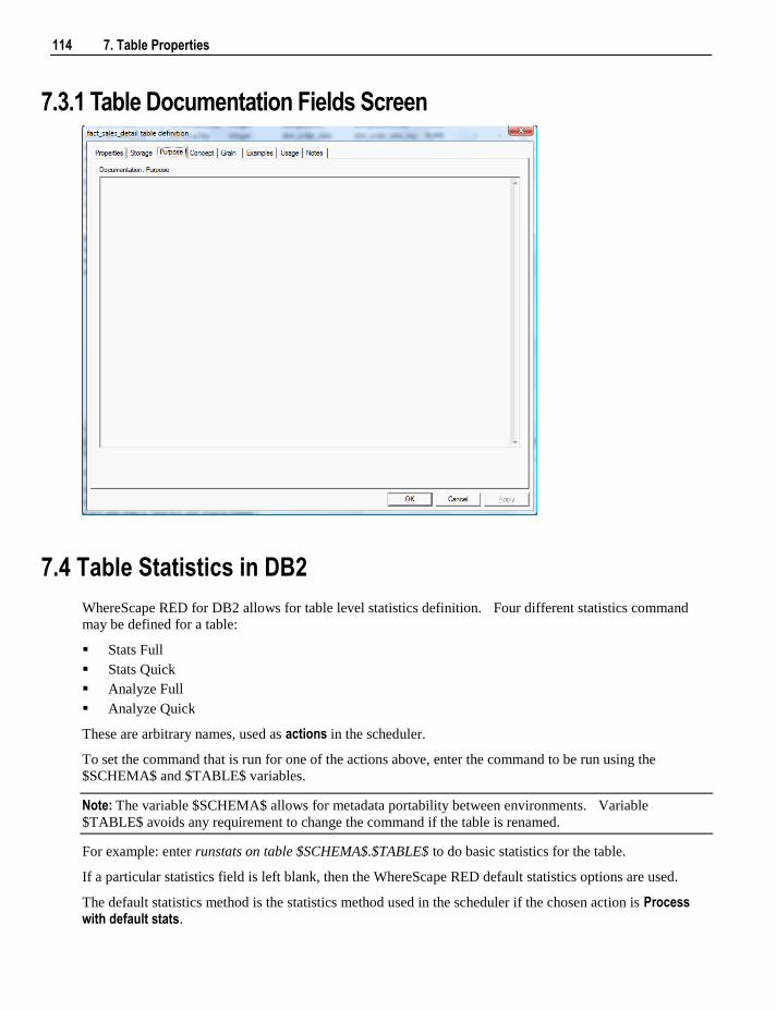
114 7. Table Properties
7.3.1 Table Documentation Fields Screen
7.4 Table Statistics in DB2
WhereScape RED for DB2 allows for table level statistics definition. Four different statistics command
may be defined for a table:
Stats Full
Stats Quick
Analyze Full
Analyze Quick
These are arbitrary names, used as actions in the scheduler.
To set the command that is run for one of the actions above, enter the command to be run using the
$SCHEMA$ and $TABLE$ variables.
Note: The variable $SCHEMA$ allows for metadata portability between environments. Variable
$TABLE$ avoids any requirement to change the command if the table is renamed.
For example: enter runstats on table $SCHEMA$.$TABLE$ to do basic statistics for the table.
If a particular statistics field is left blank, then the WhereScape RED default statistics options are used.
The default statistics method is the statistics method used in the scheduler if the chosen action is Process with default stats.
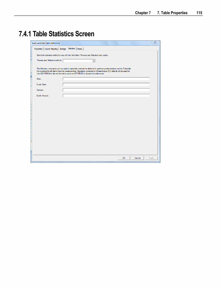
Chapter 7 7. Table Properties 115
7.4.1 Table Statistics Screen

Chapter 8 8. Loading Data 117
Load tables are the first entry point for all information coming into the data warehouse. There are multiple
ways of getting data into load tables.
Database link load - loaded from another database
Externally loaded - the load table is populated by some external process, e.g. an ETL (Extract,
Transform and Load) tool or EAI (Enterprise Application Integration) tool, putting the data directly into
the load tables.
ODBC based load - the data is loaded via an ODBC connection, either directly by reading and inserting
each row (a Load Type of ODBC load), or via a file by reading from the source system using ODBC and
writing to a file and then loading the file (a Load Type of Native ODBC). ODBC connections require a
Windows scheduler.
File load - a flat file load where most of the processing is managed and controlled by the scheduler.
Script-based load - a flat file load where a host system, i.e. Unix or Windows script file is executed to
perform the load.
XML file load - loading an XML file from a Windows directory.
In This Chapter
8.1 Choosing the Best Load Method ........................................... 118
8.2 Load Drag and Drop .............................................................. 119
8.3 Database Link Load .............................................................. 122
8.4 ODBC Based Load ................................................................ 132
8.5 SSIS Loader .......................................................................... 132
8.6 Native ODBC Based Load .................................................... 136
8.7 Flat File Loads....................................................................... 145
8.8 XML File load ....................................................................... 153
8.9 External Load ........................................................................ 156
8.10 Handling Missing Source Columns ..................................... 157
8.11 Load Table Transformations ............................................... 159
8.12 Changing Load Connection and Schema ............................ 159
C H A P T E R 8
8. Loading Data
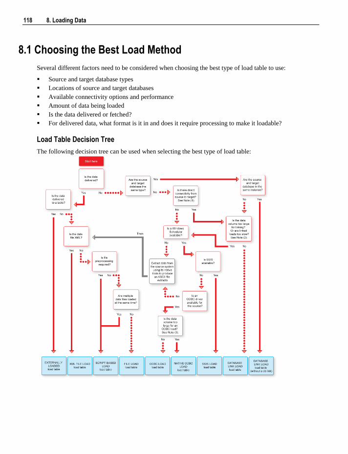
118 8. Loading Data
8.1 Choosing the Best Load Method
Several different factors need to be considered when choosing the best type of load table to use:
Source and target database types
Locations of source and target databases
Available connectivity options and performance
Amount of data being loaded
Is the data delivered or fetched?
For delivered data, what format is it in and does it require processing to make it loadable?
Load Table Decision Tree
The following decision tree can be used when selecting the best type of load table:
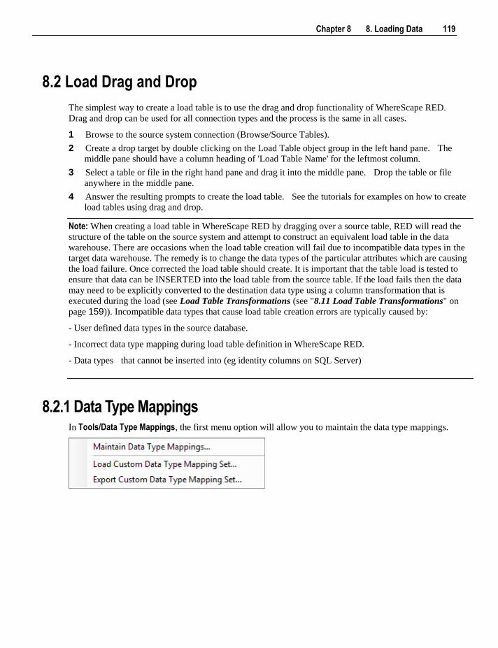
Chapter 8 8. Loading Data 119
8.2 Load Drag and Drop
The simplest way to create a load table is to use the drag and drop functionality of WhereScape RED.
Drag and drop can be used for all connection types and the process is the same in all cases.
1 Browse to the source system connection (Browse/Source Tables).
2 Create a drop target by double clicking on the Load Table object group in the left hand pane. The
middle pane should have a column heading of 'Load Table Name' for the leftmost column.
3 Select a table or file in the right hand pane and drag it into the middle pane. Drop the table or file
anywhere in the middle pane.
4 Answer the resulting prompts to create the load table. See the tutorials for examples on how to create
load tables using drag and drop.
Note: When creating a load table in WhereScape RED by dragging over a source table, RED will read the
structure of the table on the source system and attempt to construct an equivalent load table in the data
warehouse. There are occasions when the load table creation will fail due to incompatible data types in the
target data warehouse. The remedy is to change the data types of the particular attributes which are causing
the load failure. Once corrected the load table should create. It is important that the table load is tested to
ensure that data can be INSERTED into the load table from the source table. If the load fails then the data
may need to be explicitly converted to the destination data type using a column transformation that is
executed during the load (see Load Table Transformations (see "8.11 Load Table Transformations" on
page 159)). Incompatible data types that cause load table creation errors are typically caused by:
- User defined data types in the source database.
- Incorrect data type mapping during load table definition in WhereScape RED.
- Data types that cannot be inserted into (eg identity columns on SQL Server)
8.2.1 Data Type Mappings In Tools/Data Type Mappings, the first menu option will allow you to maintain the data type mappings.
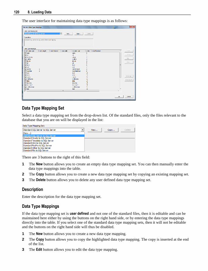
120 8. Loading Data
The user interface for maintaining data type mappings is as follows:
Data Type Mapping Set
Select a data type mapping set from the drop-down list. Of the standard files, only the files relevant to the
database that you are on will be displayed in the list:
There are 3 buttons to the right of this field:
1 The New button allows you to create an empty data type mapping set. You can then manually enter the
data type mappings into the table.
2 The Copy button allows you to create a new data type mapping set by copying an existing mapping set.
3 The Delete button allows you to delete any user defined data type mapping set.
Description
Enter the description for the data type mapping set.
Data Type Mappings
If the data type mapping set is user defined and not one of the standard files, then it is editable and can be
maintained here either by using the buttons on the right hand side, or by entering the data type mappings
directly into the table. If you select one of the standard data type mapping sets, then it will not be editable
and the buttons on the right hand side will thus be disabled.
1 The New button allows you to create a new data type mapping.
2 The Copy button allows you to copy the highlighted data type mapping. The copy is inserted at the end
of the list.
3 The Edit button allows you to edit the data type mapping.
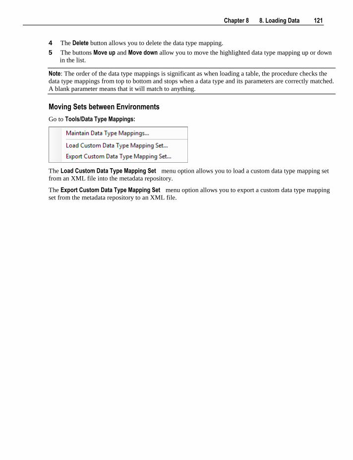
Chapter 8 8. Loading Data 121
4 The Delete button allows you to delete the data type mapping.
5 The buttons Move up and Move down allow you to move the highlighted data type mapping up or down
in the list.
Note: The order of the data type mappings is significant as when loading a table, the procedure checks the
data type mappings from top to bottom and stops when a data type and its parameters are correctly matched.
A blank parameter means that it will match to anything.
Moving Sets between Environments
Go to Tools/Data Type Mappings:
The Load Custom Data Type Mapping Set menu option allows you to load a custom data type mapping set
from an XML file into the metadata repository.
The Export Custom Data Type Mapping Set menu option allows you to export a custom data type mapping
set from the metadata repository to an XML file.
122 8. Loading Data
8.3 Database Link Load
8.3.1 Database Link Load - Properties The fields on the Load Table Properties screen (see "8.3.1.1 Load Table Properties Screen" on page 124)
for database link loads are described below:
Load Table Name
The table name is limited by most relational databases to a maximum of 30 characters and must be unique.
Table name defaults can be set up (Tools/Options) to define a prefix or a post fix that can be added in order
to identify clearly that this is a load table. Example: load_customer. By default WhereScape RED uses
the prefix load_ for load tables.
Short Name
The table short name is limited in size to 22 characters in Oracle and SQL Server and 12 characters in DB2.
It must be unique. The short name is used in the naming of indexes, keys, procedures and scripts.
Description
Enter here a description of the table. This description appears in the documentation that can be generated
once the data warehouse is built.
Connection
Enter the connection being used to get the data. The connections for load tables can be changed on bulk
see Changing load Connection and Schema (see "8.12 Changing Load Connection and Schema" on page
159).
Load Type
The load type is typically defined by the connection, and should not normally be changed. This drop down
shows all valid load types for the connection.
Database Link
The database link will display in this field.
Script Name
This field is only active if this is a script based load.
Pre-load Action
Select an action to be performed on the table before the load occurs. Options are:
Truncate
Execute pre-load Sql
Both Truncate and Execute pre-load Sql
No action
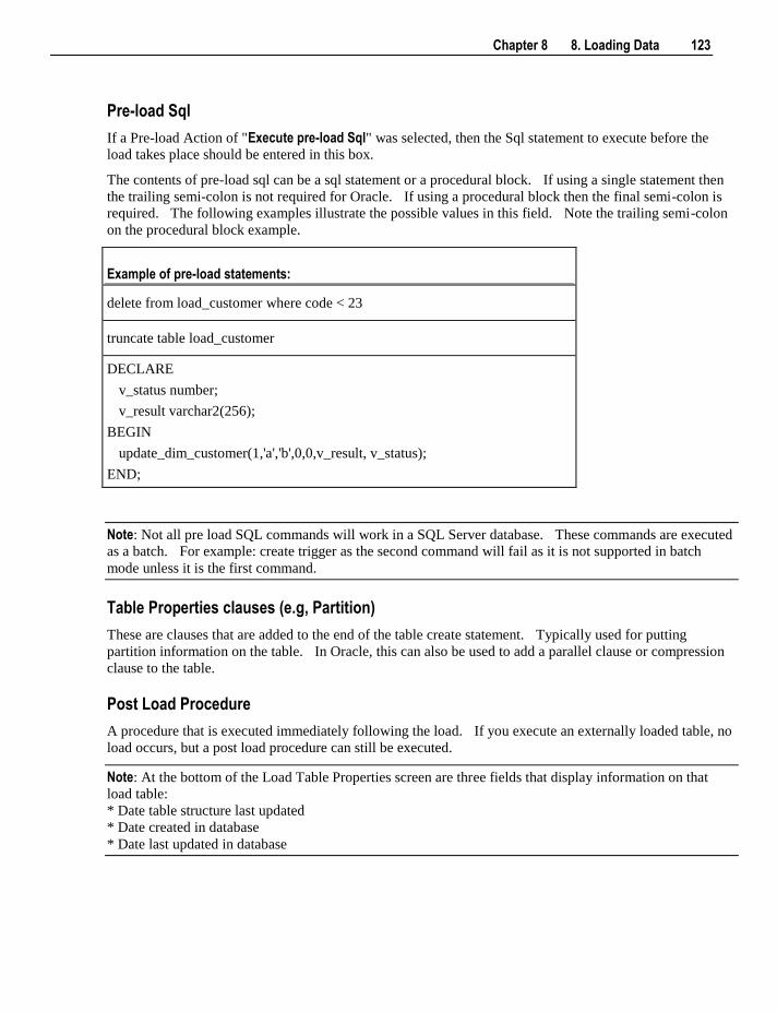
Chapter 8 8. Loading Data 123
Pre-load Sql
If a Pre-load Action of "Execute pre-load Sql" was selected, then the Sql statement to execute before the
load takes place should be entered in this box.
The contents of pre-load sql can be a sql statement or a procedural block. If using a single statement then
the trailing semi-colon is not required for Oracle. If using a procedural block then the final semi-colon is
required. The following examples illustrate the possible values in this field. Note the trailing semi-colon
on the procedural block example.
Example of pre-load statements:
delete from load_customer where code < 23
truncate table load_customer
DECLARE
v_status number;
v_result varchar2(256);
BEGIN
update_dim_customer(1,'a','b',0,0,v_result, v_status);
END;
Note: Not all pre load SQL commands will work in a SQL Server database. These commands are executed
as a batch. For example: create trigger as the second command will fail as it is not supported in batch
mode unless it is the first command.
Table Properties clauses (e.g, Partition)
These are clauses that are added to the end of the table create statement. Typically used for putting
partition information on the table. In Oracle, this can also be used to add a parallel clause or compression
clause to the table.
Post Load Procedure
A procedure that is executed immediately following the load. If you execute an externally loaded table, no
load occurs, but a post load procedure can still be executed.
Note: At the bottom of the Load Table Properties screen are three fields that display information on that
load table:
* Date table structure last updated
* Date created in database
* Date last updated in database
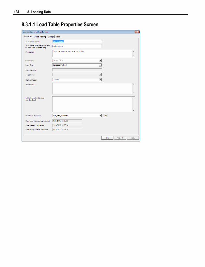
124 8. Loading Data
8.3.1.1 Load Table Properties Screen
Chapter 8 8. Loading Data 125
8.3.2 Database Link Load - Source Mapping The fields on the Load Table Source Mapping tab (see "8.3.2.1 Load Table Source Mapping Screen" on
page 127) of the properties screen for database link loads are described below:
Source schema
This displays the schema in the source database (where the data is coming from).
Source table name(s)
The name of the table or tables that the data is coming from.
Non mandatory source columns
This box can only be checked if the Use Source column/transformation checkbox is checked. When the non
mandatory source columns checkbox is selected WhereScape RED will process the load even when one or
more of the source columns does not exist. In this way a super set of source columns can be selected
across different versions of an application. If this option is chosen it may be advisable to set a default
value via a transformation if the column is null. (see the section on handling missing source columns (see
"8.10 Handling Missing Source Columns" on page 157)).
Note: This option is only available in Oracle.
Exit status when missing columns
If non mandatory source columns are detected how should the load exit? Options are success, warning or
error.
Load Type
The load type field can be used to reduce database logging in DB2. The default is to reduce logging and to
not provide for full recovery. The two options are:
Minimal Logging.
Recoverable Load.
Note: This option is only available in DB2.
Load Modifier
This option only applies if Minimal Logging is used in DB2. It allows for a LOAD statement load modifier
to be added to the load.
Note: This option is only available in DB2.
Distinct data select
If checked, the keyword DISTINCT is added to the select statement.
Insert Hint
126 8. Loading Data
A database hint to include when running the insert statement for the load table.
Note: This option is only available in SQL Server.
Use Source column/transformation checkbox
If this box is checked then WhereScape RED uses the information stored against each column rather than
the source columns as below. See the section on transformation (see "8.11 Load Table Transformations"
on page 159) below for a fuller explanation.
Source columns
The names of the columns that the data is coming from.
TIP: When a table is created, by default WhereScape RED populates the fields Source table names
and Source columns which show where each column came from. At the top right of the screen is a button
called Update columns and tables from the table column mappings. If you click on this button you can
update the Source table name and columns based on this information that is stored against each column.
This will overwrite whatever is currently in those two fields.
Where, Group etc. clauses:
WhereScape RED builds a select statement (SELECT * from [table name]). The Where or Group clauses
are those clauses that immediately follow the from verb of the select statement. For example: SELECT *
from Customer WHERE rownum < 300.
TIP: This is where you can build a statement to handle change data.
Parameter values can be in-line replaced and included in the where clause. Prefix the parameter name with
a '$P' and add a trailing '$'. For example if we have a parameter called SALES_LOCATION_CODE we
could construct a statement such as WHERE location_code = '$PSALES_LOCATION_CODE$' AND
region_code = 'NZ'. When this statement is executed the value of the parameter will replace the parameter
name. For example if the parameter was set to 'Auckland' then the statement would execute as: WHERE
location_code = 'Auckland' AND region_code = 'NZ'.
Remote view name
If a name is entered in this field, WhereScape RED will try and create a view over on the remote system
and then extract from that view. If you enter a remote view name you must enter a remote view where
clause. The remote view creation procedure must exist on the source system. See Remote View Extract
(see "8.3.3 Remote View Extract" on page 129) topic.
Note: Remote view name and the view where clause are only available in Oracle.
Where clause (for Remote view)
These are typically the same as the Where clauses above, but may prefix table names or schemas.
Parameter values can be in-line replaced and included in the where clause. See the example above in the
'Where, Group etc. clauses section'.
Load Statement
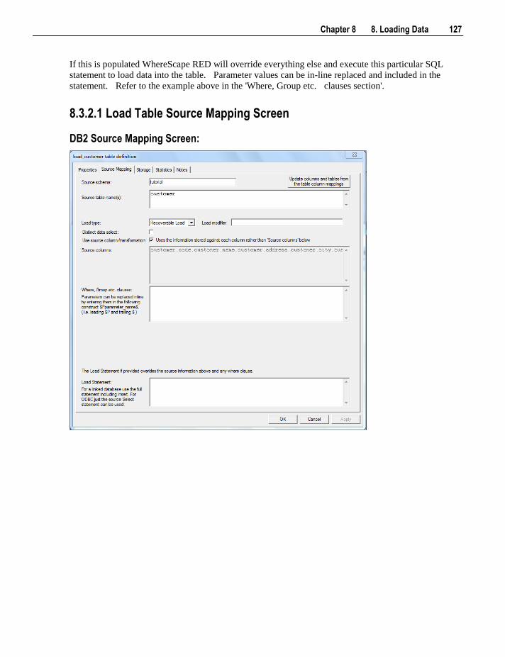
Chapter 8 8. Loading Data 127
If this is populated WhereScape RED will override everything else and execute this particular SQL
statement to load data into the table. Parameter values can be in-line replaced and included in the
statement. Refer to the example above in the 'Where, Group etc. clauses section'.
8.3.2.1 Load Table Source Mapping Screen
DB2 Source Mapping Screen:
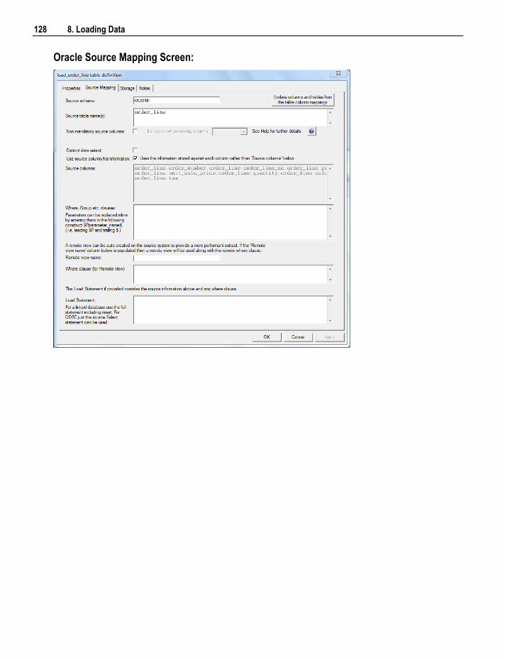
128 8. Loading Data
Oracle Source Mapping Screen:
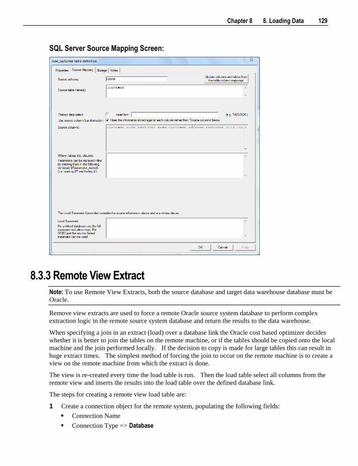
Chapter 8 8. Loading Data 129
SQL Server Source Mapping Screen:
8.3.3 Remote View Extract
Note: To use Remote View Extracts, both the source database and target data warehouse database must be
Oracle.
Remove view extracts are used to force a remote Oracle source system database to perform complex
extraction logic in the remote source system database and return the results to the data warehouse.
When specifying a join in an extract (load) over a database link the Oracle cost based optimizer decides
whether it is better to join the tables on the remote machine, or if the tables should be copied onto the local
machine and the join performed locally. If the decision to copy is made for large tables this can result in
huge extract times. The simplest method of forcing the join to occur on the remote machine is to create a
view on the remote machine from which the extract is done.
The view is re-created every time the load table is run. Then the load table select all columns from the
remote view and inserts the results into the load table over the defined database link.
The steps for creating a remote view load table are:
1 Create a connection object for the remote system, populating the following fields:
Connection Name
Connection Type => Database
130 8. Loading Data
ODBC Source
Database id (SID)
Database link id
Extract user name
Extract password
2 Ensure the user name and password being used to connect to the remote system have the following
privileges:
create view (granted as a specific privilege and not part of a role)
compile procedure (granted as a specific privilege and not part of a role)
execute on sys.dbms_sql
3 Right click on the connection to the remote system and choose Create Database Link. When the dialog
with the database link has been created message is displayed, click OK.
4 Right click on the connection to the remote system and choose Create remote view procedure. When
the dialog with the Procedure dss_view_compile compiled is displayed, click OK.
5 Browse the connection in the right hand pane.
6 Drag and drop a source table or columns of the source tables to create the required load table.
7 Create the load table in the data warehouse database by selecting Create (Recreate) from the right click
menu.
8 Right click on the load table and select Source Mapping.
9 Enter a name for the remote view to be created into the Remote view name box. For example, use the
name of the load table.
10 Cut or copy any existing where clause from the Where, Group etc. clauses box and paste it into the
Where clause (for Remote view) box. Alternatively, enter the where clause (including any table joins, if
multiple source tables are being extracted from) into the Where clause (for Remote view) box.
Note: Once the load table has a remote view name, the where clause in the Where, Group etc. clauses
box is ignored and the where clause in the Where clause (for Remote view) box is used instead.
11 Click OK.
12 Load or schedule the load table.
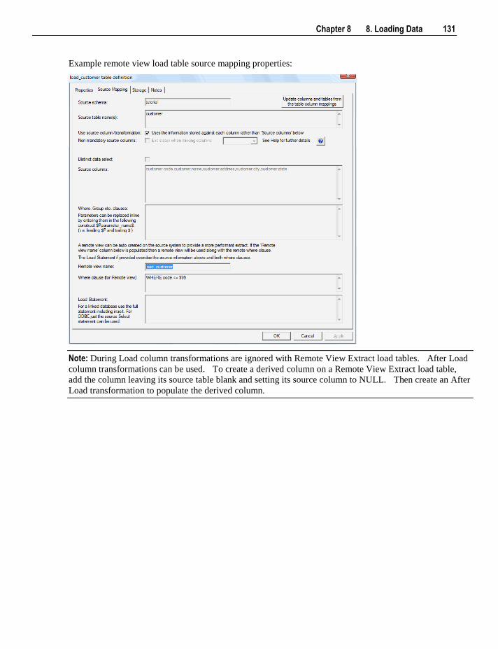
Chapter 8 8. Loading Data 131
Example remote view load table source mapping properties:
Note: During Load column transformations are ignored with Remote View Extract load tables. After Load
column transformations can be used. To create a derived column on a Remote View Extract load table,
add the column leaving its source table blank and setting its source column to NULL. Then create an After
Load transformation to populate the derived column.
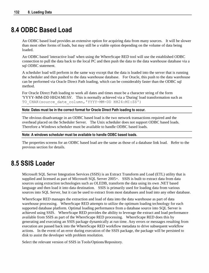
132 8. Loading Data
8.4 ODBC Based Load
An ODBC based load provides an extensive option for acquiring data from many sources. It will be slower
than most other forms of loads, but may still be a viable option depending on the volume of data being
loaded.
An ODBC based 'interactive load' when using the WhereScape RED tool will use the established ODBC
connection to pull the data back to the local PC and then push the data to the data warehouse database via a
sql ODBC statement.
A scheduler load will perform in the same way except that the data is loaded into the server that is running
the scheduler and then pushed to the data warehouse database. For Oracle, this push to the data warehouse
can be performed via Oracle Direct Path loading, which can be considerably faster than the ODBC sql
method.
For Oracle Direct Path loading to work all dates and times must be a character string of the form
'YYYY-MM-DD HH24:MI:SS'. This is normally achieved via a 'During' load transformation such as TO_CHAR(source_date_column,'YYYY-MM-DD HH24:MI:SS')
Note: Dates must be in the correct format for Oracle Direct Path loading to occur.
The obvious disadvantage in an ODBC based load is the two network transactions required and the
overhead placed on the Scheduler Server. The Unix scheduler does not support ODBC based loads.
Therefore a Windows scheduler must be available to handle ODBC based loads.
Note: A windows scheduler must be available to handle ODBC based loads.
The properties screens for an ODBC based load are the same as those of a database link load. Refer to the
previous section for details.
8.5 SSIS Loader
Microsoft SQL Server Integration Services (SSIS) is an Extract Transform and Load (ETL) utility that is
supplied and licensed as part of Microsoft SQL Server 2005+. SSIS is built to extract data from data
sources using extraction technologies such as OLEDB, transform the data using its own .NET based
language and then load it into data destination. SSIS is primarily used for loading data from various
sources into SQL Server, but it can be used to extract from most databases and load into any other database.
WhereScape RED manages the extraction and load of data into the data warehouse as part of data
warehouse processing. WhereScape RED attempts to utilize the optimum loading technology for each
supported database platform. Optimal loading performance from a database source into SQL Server is
achieved using SSIS. WhereScape RED provides the ability to leverage the extract and load performance
available from SSIS as part of the WhereScape RED processing. WhereScape RED does this by
generating and executing an SSIS package dynamically at run time. Any errors or messages resulting from
execution are passed back into the WhereScape RED workflow metadata to drive subsequent workflow
actions. In the event of an error during execution of the SSIS package, the package will be persisted to
disk to assist the developer with problem resolution.
Select the relevant version of SSIS in Tools/Options/Repository.
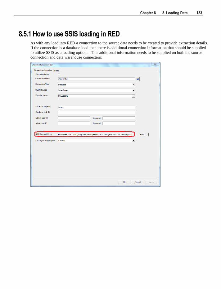
Chapter 8 8. Loading Data 133
8.5.1 How to use SSIS loading in RED As with any load into RED a connection to the source data needs to be created to provide extraction details.
If the connection is a database load then there is additional connection information that should be supplied
to utilize SSIS as a loading option. This additional information needs to be supplied on both the source
connection and data warehouse connection:
134 8. Loading Data
SSIS Connect String is a valid SSIS connection string that can be used to connect to the data source or
destination. The Reset button will attempt to construct a valid connection string from the connection
information supplied in the connection details consisting of the Database ID, Database Link ID (Instance
name), Provider Name, Extract User details.
Once the connection is defined then a load table needs to be created to hold data landed into the data
warehouse by dragging a source table to create a load table. (see Loading data (see "8. Loading Data" on
page 117) ) On the load table properties the Load type can be set to Integration Services (Beta). This will
create and execute a SSIS package at run time to load data into the data warehouse load table.
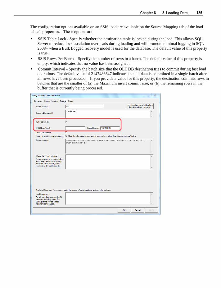
Chapter 8 8. Loading Data 135
The configuration options available on an SSIS load are available on the Source Mapping tab of the load
table‟s properties. These options are:
SSIS Table Lock - Specify whether the destination table is locked during the load. This allows SQL
Server to reduce lock escalation overheads during loading and will promote minimal logging in SQL
2008+ when a Bulk Logged recovery model is used for the database. The default value of this property
is true.
SSIS Rows Per Batch – Specify the number of rows in a batch. The default value of this property is
empty, which indicates that no value has been assigned.
Commit Interval - Specify the batch size that the OLE DB destination tries to commit during fast load
operations. The default value of 2147483647 indicates that all data is committed in a single batch after
all rows have been processed. If you provide a value for this property, the destination commits rows in
batches that are the smaller of (a) the Maximum insert commit size, or (b) the remaining rows in the
buffer that is currently being processed.

136 8. Loading Data
8.5.2 Troubleshooting If an SSIS load fails due to incorrect connection strings then the SSIS package will fail to create at run time.
The connection string information in both the source connection and the data warehouse connection (the
destination) should be checked to ensure that they are correct.
If the SSIS load fails due to incorrect extraction SQL, due to mismatched destination load table structure or
due to constraint violation then the SSIS package will be created in the file system for the developer to
check. The SSIS package file will be created in the WhereScape RED Work Directory (shown in the
dialog opened from the WhereScape RED menu item Tools / Object Count ). This SSIS package will have
a DTSX file extension and can be opened using the appropriate version of Microsoft‟s BI Development
Studio add-in to Visual Studio.
8.6 Native ODBC Based Load
A Native ODBC based load is similar to an ODBC load, except it provides a faster method to load data
from non-linked databases.
A Native ODBC based 'interactive load' when using the WhereScape RED tool will use the established
ODBC connection to pull the data back to a delimited file on the local PC and then push the data to the data
warehouse database via a Bulk Insert in SQL Server, SQL*LOADER in Oracle or LOAD statement in
DB2.
A scheduler load will perform in the same way except that the data is loaded into the server that is running
the scheduler and then pushed to the data warehouse database.
All loaders require dates in the default format of the target data warehouse database. This is normally
achieved via a 'During' load transformation using the correct casting function for the source database.
The properties and storage screens for a Native ODBC based load are the same as those of a database link
load. Refer to the previous section for details. Details of the source mapping screen follow.
Native Loads in Oracle
Some versions of Oracle do not return the ORACLE_SID correctly when an ODBC call requests it. To
ensure that you don't have any issues because of this, please ensure that the following steps are followed:
If you are doing interactive Native Loads in RED into Oracle:
1 Ensure that the "Database id (SID)" field on the Data Warehouse connection properties screen is set to
the actual ORACLE_SID for your database.
This value is used in the sqlldr connection during the native load IF the ORACLE_SID is not returned
correctly by the ODBC driver.
If you are using the windows scheduler for Native Loads into Oracle:
1 Change the scheduler to be a direct path load (via maintain scheduler in the WhereScape
Administrator).
2 Ensure that the TNS Service is set to the actual ORACLE_SID for your database.
3 Restart the scheduler.
Chapter 8 8. Loading Data 137
This value is used in the sqlldr connection IF the SID is not returned by the ODBC driver and only IF the
scheduler is set to do direct path loads.
138 8. Loading Data
8.6.1 Native ODBC Based Load - Source Mapping The fields on the Source Mapping tab of the properties screen for Native ODBC loads are described below:
Source schema
This displays the source database where the data is coming from.
Source table name(s)
The name of the table or tables that the data is coming from.
Non mandatory source columns
This box can only be checked if the Use Source column/transformation checkbox is checked. When the non
mandatory source columns checkbox is selected WhereScape RED will process the load even when one or
more of the source columns does not exist. In this way a super set of source columns can be selected
across different versions of an application. If this option is chosen it may be advisable to set a default
value via a transformation if the column is null. (see the section on handling missing source columns (see
"8.10 Handling Missing Source Columns" on page 157)).
Note: This option only applies to Oracle.
Exit status when missing columns
If Non mandatory source columns are detected how should the load exit. Options are success, warning or
error. This only applies to Oracle.
Native Load Routine
Choose the databases file loading routine. In some databases there may be only one Native Routine
available.
Native Load Delimiter
The native load delimiter is used to specify the character used as the delimiter of the extract file that is built
during the load. The default value is a | character (pipe). This should be changed if pipes are possible in
the source data.
UNICODE extract file
If you create a native ODBC load from any database containing UNICODE characters, then this field must
be checked.The default is unchecked and this field is not available on DB2.
Distinct data select
If checked, the keyword DISTINCT is added to the select statement.
Use Source column/transformation check box
If this box is checked then WhereScape RED uses the information stored against each column rather than
the source columns as below. See the section on Load Table Transformations (see "8.11 Load Table
Transformations" on page 159) below for a fuller explanation.
Chapter 8 8. Loading Data 139
Source columns
The names of the columns that the data is coming from.
TIP: When a table is created, by default WhereScape RED populates the fields Source table names
and Source columns which show where each column came from. At the top right of the screen is a button
called Update columns and tables from the table column mappings. If you click this button you can update
the Source table name and columns based on this information that is stored against each column. This will
overwrite whatever is currently in those two fields.
Where, Group etc. clauses:
WhereScape RED builds a select statement (SELECT * from [table name]). The Where or Group clauses
are those clauses that immediately follow the from verb of the select statement. For example: SELECT *
from Customer WHERE code > 225.
TIP: This is where you can build a statement to handle change data.
Parameter values can be in-line replaced and included in the where clause. Prefix the parameter name with
a '$P' and add a trailing '$'. For example if we have a parameter called SALES_LOCATION_CODE we
could construct a statement such as WHERE location_code = '$PSALES_LOCATION_CODE$' AND
region_code = 'NY'. When this statement is executed the value of the parameter will replace the parameter
name. For example if the parameter was set to 'New York' then the statement would execute as: WHERE
location_code = 'New York' AND region_code = 'US'.
Remote view name
If a name is entered in this field, WhereScape RED will try and create a view over on the remote system
and then extract from that view. If you enter a remote view name you must enter a remote view where
clause. The remote view creation procedure must exist on the source system. See Remote View Extract
(see "8.3.3 Remote View Extract" on page 129) topic.
Note: Remote view name and the view where clause are only available in Oracle.
Where clause (for Remote view)
These are typically the same as the Where clauses above, but may prefix table names or schemas.
Parameter values can be in-line replaced and included in the where clause. See the example above in the
'Where, Group etc. clauses section'.
Load Statement
If this is populated WhereScape RED will override everything else and execute this particular SQL
statement to load data into the table. Parameter values can be in-line replaced and included in the
statement. Refer to the example above in the 'Where, Group etc. clauses section'.
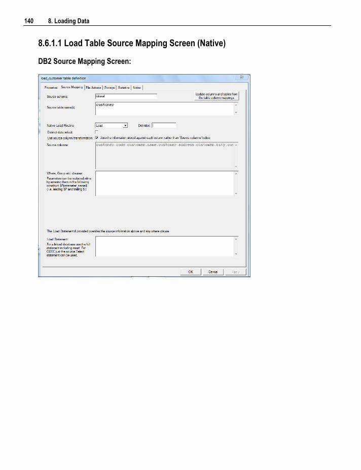
140 8. Loading Data
8.6.1.1 Load Table Source Mapping Screen (Native)
DB2 Source Mapping Screen:
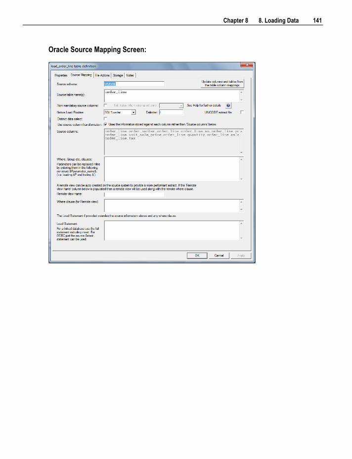
Chapter 8 8. Loading Data 141
Oracle Source Mapping Screen:
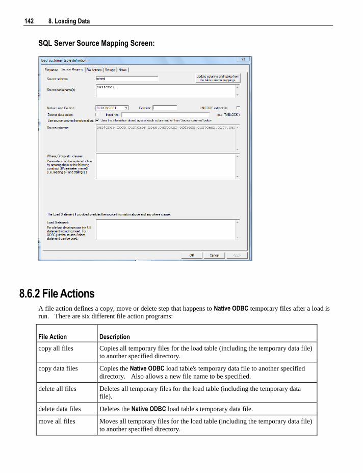
142 8. Loading Data
SQL Server Source Mapping Screen:
8.6.2 File Actions A file action defines a copy, move or delete step that happens to Native ODBC temporary files after a load is
run. There are six different file action programs:
File Action Description
copy all files Copies all temporary files for the load table (including the temporary data file)
to another specified directory.
copy data files Copies the Native ODBC load table's temporary data file to another specified
directory. Also allows a new file name to be specified.
delete all files Deletes all temporary files for the load table (including the temporary data
file).
delete data files Deletes the Native ODBC load table's temporary data file.
move all files Moves all temporary files for the load table (including the temporary data file)
to another specified directory.
Chapter 8 8. Loading Data 143
move data files Moves the Native ODBC load table's temporary data file to another specified
directory. Also allows a new file name to be specified.
Note: A load table may have more than one file action. File actions are processed in order, based on the
action number.
Creating a File Action
To create a file action:
1 Click on the File Actions tab of the load table properties dialog.
2 Click the Add new action button.
3 Choose After load from the Action Type drop down list.
4 Enter the Action Description.
5 Choose the Action Program from the drop down list (see above for the options).
6 For action programs of copy... and move..., enter the target directory name.
7 For copy data files and move data files, optionally enter the file's new name.
8 Click on Save / update action.
9 Repeat if necessary for additional file actions.
10 Click OK.
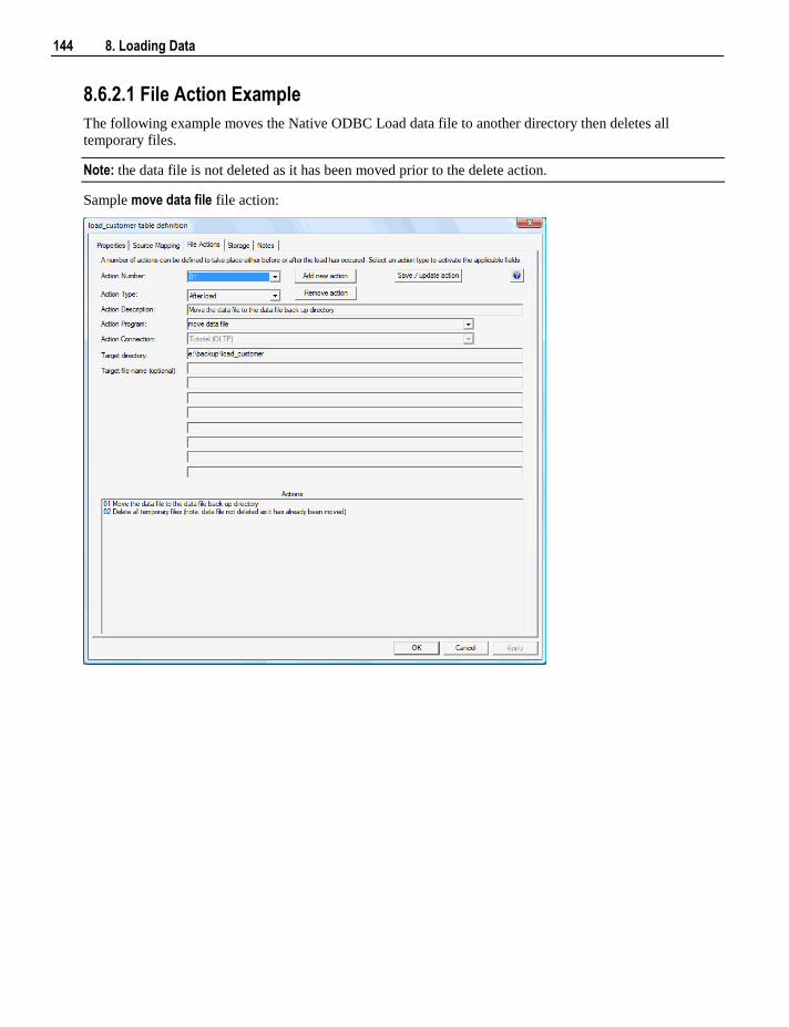
144 8. Loading Data
8.6.2.1 File Action Example
The following example moves the Native ODBC Load data file to another directory then deletes all
temporary files.
Note: the data file is not deleted as it has been moved prior to the delete action.
Sample move data file file action:
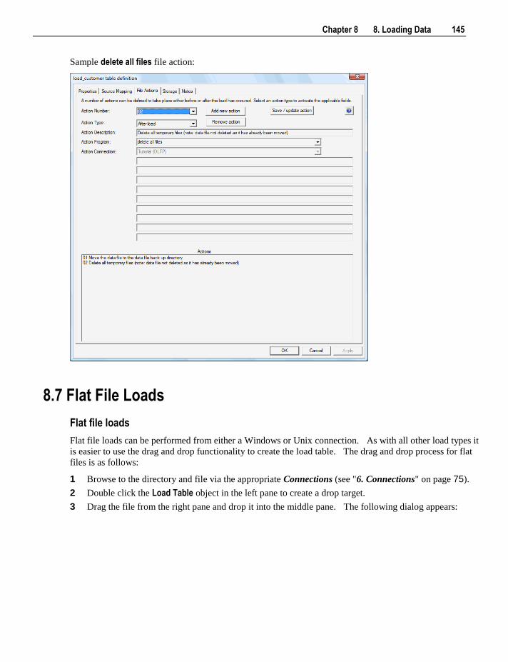
Chapter 8 8. Loading Data 145
Sample delete all files file action:
8.7 Flat File Loads
Flat file loads
Flat file loads can be performed from either a Windows or Unix connection. As with all other load types it
is easier to use the drag and drop functionality to create the load table. The drag and drop process for flat
files is as follows:
1 Browse to the directory and file via the appropriate Connections (see "6. Connections" on page 75).
2 Double click the Load Table object in the left pane to create a drop target.
3 Drag the file from the right pane and drop it into the middle pane. The following dialog appears:
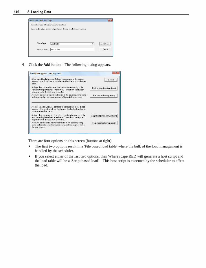
146 8. Loading Data
4 Click the Add button. The following dialog appears.
There are four options on this screen (buttons at right).
The first two options result in a 'File based load table' where the bulk of the load management is
handled by the scheduler.
If you select either of the last two options, then WhereScape RED will generate a host script and
the load table will be a 'Script based load'. This host script is executed by the scheduler to effect
the load.
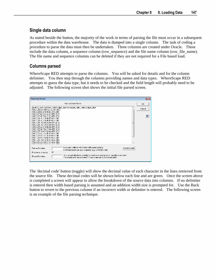
Chapter 8 8. Loading Data 147
Single data column
As stated beside the button, the majority of the work in terms of parsing the file must occur in a subsequent
procedure within the data warehouse. The data is dumped into a single column. The task of coding a
procedure to parse the data must then be undertaken. Three columns are created under Oracle. These
include the data column, a sequence column (row_sequence) and the file name column (row_file_name).
The file name and sequence columns can be deleted if they are not required for a File based load.
Columns parsed
WhereScape RED attempts to parse the columns. You will be asked for details and for the column
delimiter. You then step through the columns providing names and data types. WhereScape RED
attempts to guess the data type, but it needs to be checked and the field length will probably need to be
adjusted. The following screen shot shows the initial file parsed screen.
The 'decimal code' button (toggle) will show the decimal value of each character in the lines retrieved from
the source file. These decimal codes will be shown below each line and are green. Once the screen above
is completed a screen will appear to allow the breakdown of the source data into columns. If no delimiter
is entered then width based parsing is assumed and an addition width size is prompted for. Use the Back
button to revert to the previous column if an incorrect width or delimiter is entered. The following screen
is an example of the file parsing technique.
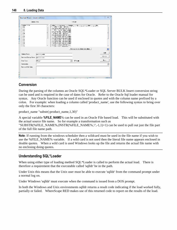
148 8. Loading Data
Conversion
During the parsing of the columns an Oracle SQL*Loader or SQL Server BULK Insert conversion string
can be used and is required in the case of dates for Oracle. Refer to the Oracle Sql loader manual for
syntax. Any Oracle function can be used if enclosed in quotes and with the column name prefixed by a
colon. For example: when loading a column called 'product_name', use the following syntax to bring over
only the first 30 characters:
product_name "substr(:product_name,1,30)"
A special variable %FILE_NAME% can be used in an Oracle File based load. This will be substituted with
the actual source file name. So for example a transformation such as
"SUBSTR(%FILE_NAME%,INSTR(%FILE_NAME%,'/',-1,1)+1) can be used to pull out just the file part
of the full file name path.
Note: If running from the windows scheduler then a wildcard must be used in the file name if you wish to
use the %FILE_NAME% variable. If a wild card is not used then the literal file name appears enclosed in
double quotes. When a wild card is used Windows looks up the file and returns the actual file name with
no enclosing doing quotes.
Understanding SQL*Loader
When using either type of loading method SQL*Loader is called to perform the actual load. There is
therefore a requirement that the executable called 'sqlldr' be in the path.
Under Unix this means that the Unix user must be able to execute 'sqlldr' from the command prompt under
a normal log on.
Under Windows 'sqlldr' must execute when the command is issued from a DOS prompt.
In both the Windows and Unix environments sqlldr returns a result code indicating if the load worked fully,
partially or failed. WhereScape RED makes use of this returned code to report on the results of the load.
Chapter 8 8. Loading Data 149
8.7.1 File Load When a file based load table is created a different tab is displayed on the properties screen. This is the File Attributes tab (see "8.7.1.1 Load Table File Attributes Screen" on page 151). The fields are described below:
TIP: If the file has been dragged and dropped (see "8.7 Flat File Loads" on page 145) into the load
table (middle pane) then some of the fields on this tab are automatically populated.
File Path
The full path name to the directory in which the file is located on the Windows or Unix system.
File Name
The name of the file in the directory.
File Column Delimiter
Any delimiter in the file that splits out the columns, e.g, a comma (,). Note that if an ASCII character
value is used this field may show as an unprintable character. To enter a special character enter the
uppercase string CHAR with the ASCII value in brackets (e.g. CHAR(9) ).
Optionally enclosed by
Oracle Only. Allows the entry of an optionally enclosed by statement in SQL*Loader. Normally this will
be a double quote
File has a Header line
If the file has a header line and this checkbox is ticked, then WhereScape RED will drop the first line from
the load.
File Record Delimiter
Enter the record delimiter of FIXnnn to specify a fixed length record. By default the delimiter is a newline
(\n). If no delimiters are used then enter the width of the record (e.g. FIX80 for a 80 byte record).
Sql loader options
Oracle only. Allows the entry of both SQL*Loader options and a 'When' statement. If both options and a
when statement are used then the when statement must follow the options. (e.g. options
(direct=true,parallel=true) when product_code = '02' ).
Note: There are some limitations on the 'When statement'. At the time of writing the not symbol (!) will not
work for a Windows based load but will work under Unix.
BULK INSERT options
150 8. Loading Data
SQL Server only. Allows the entry of both BULK INSERT options. For Example: to ensure a lock is
place on a table enter TABLOCK, to set the batch size for the load to 100000 rows enter BATCHSIZE=100000,
to make bulk insert error on the first row, enter MAXERRORS=0. Separate multiple values using commas.
LOAD options
DB2 only. Allow the entry of options for the LOAD statement. By default, this field is populated with
the NONRECOVERABLE option. This may be removed if not required.
LOAD modifier
DB2 only. Allow the entry of modifiers for the LOAD statement. By default, this field is populated with
the TIMESTAMPFORMAT option set. This may be modified or removed.
Wait seconds
Enter a time here, being the number of seconds to wait for a file, e.g, 1800 seconds. A value of 0 equates
to no wait. If the wait time expires and the specified file cannot be found, then the load will exit with the
status defined in Action, e.g, Default Action = Error
Action on wait expire
This will enable a scheduled job to continue if the file was not found within the wait period. If the action
chosen is success or warning then the scheduler will continue to run other scheduled tasks. An error will
cause the scheduler to stop the job and hold any remaining tasks.
Trigger Path
The purpose of the trigger file is to indicate that the copying / loading of the main file has completed and
that it is now safe to load the file. Secondly the trigger file may contain control sums to validate the
contents of the main load file. This field should contain the full path name to the directory in which a
trigger file is located on the Windows or Unix systems. If this field and/or the 'Trigger Name' field is
populated then the scheduler will look for this file rather than the actual load file.
Trigger Name
Refers to the name of the file that is used as a trigger to indicate that the main load file is available. A
trigger file typically contains check sums. If the trigger file exists then this is the file that is used in the
Wait Seconds, and Action on wait expire processing. (see notes under Trigger Path above).
Trigger Delimiter
If the trigger file provides control information then the delimiter identifies the field separation, e.g , or \n
for a return. The data found will be loaded into parameter values whose names will be prefixed by the
prefix specified and numbered 0 to n.
Trigger Parameter Prefix
If a trigger file and delimiter have been specified then the contents of the trigger file are loaded into
parameters. The parameters will be prefixed by the contents of this field and suffixed by an underscore
and the parameter number. These parameters can be viewed under ( Tools / Parameters ) from the
WhereScape RED menu bar. The checking of these parameters can be achieved by generating a 'Post Load
procedure'. An example set of parameters may be budget_0, budget_1 and budget_2 where there are 3
values in the trigger file and the prefix is set to 'budget'.
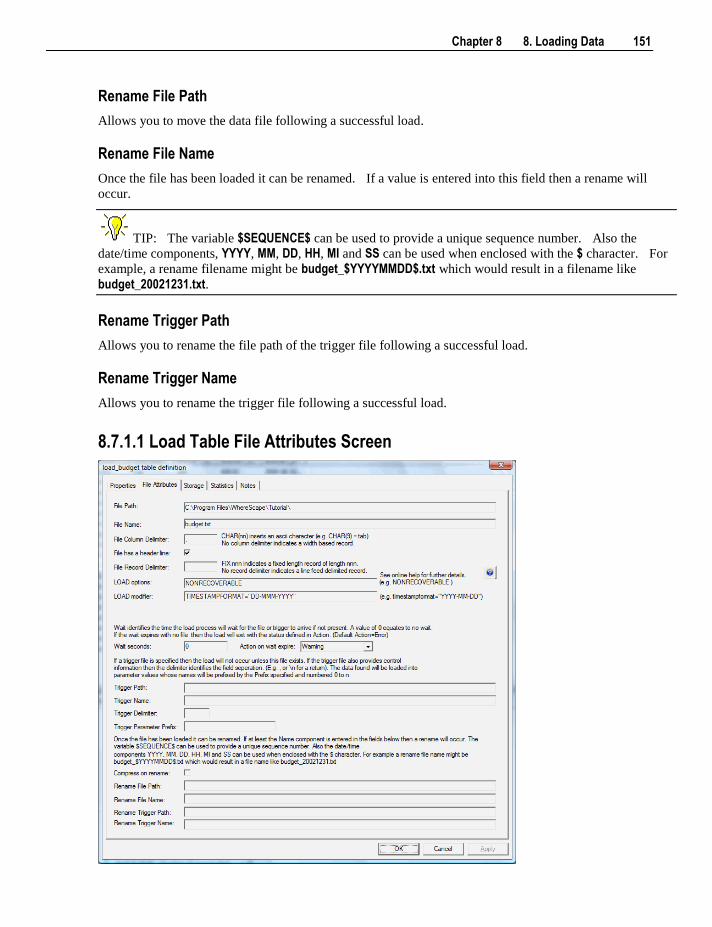
Chapter 8 8. Loading Data 151
Rename File Path
Allows you to move the data file following a successful load.
Rename File Name
Once the file has been loaded it can be renamed. If a value is entered into this field then a rename will
occur.
TIP: The variable $SEQUENCE$ can be used to provide a unique sequence number. Also the
date/time components, YYYY, MM, DD, HH, MI and SS can be used when enclosed with the $ character. For
example, a rename filename might be budget_$YYYYMMDD$.txt which would result in a filename like
budget_20021231.txt.
Rename Trigger Path
Allows you to rename the file path of the trigger file following a successful load.
Rename Trigger Name
Allows you to rename the trigger file following a successful load.
8.7.1.1 Load Table File Attributes Screen
152 8. Loading Data
8.7.2 Host Script Loads A script based load table will have a Host Script defined. During the load process this host script is
executed and the results returned.
During the 'drag and drop' creation of a load table from a Unix or Windows file a script can be generated by
selecting one of the 'Script based' load options. This script can then be edited to more fully meet any
requirements.
Note: If the Unix Scheduler is not being used and a Unix script is generated and executed interactively the
following two variables will be setup as part of the environment.
DSS_USER=username
DSS_PWD=password
Where 'username' and 'password' are the entries for the data warehouse database.
There are a number of conventions that must be followed if these host scripts are to be used by the
WhereScape scheduler.
1 The first line of data in 'standard out' must contain the resultant status of the script. Valid values are '1'
to indicate success, '-1' to indicate a Warning condition occurred but the result is considered a success,
'-2' to indicate a handled Error occurred and subsequent dependent tasks should be held, -3 to indicate
an unhandled Failure and that subsequent dependent tasks should be held.
2 The second line of data in 'standard out' must contain a resultant message of no more than 256
characters.
3 Any subsequent lines in 'standard out' are considered informational and are recorded in the audit trail.
The normal practice is to place a minimum of information in the audit trail. All bulk information
should be output to 'standard error'
4 Any data output to 'standard error' will be written to the error/detail log. Both the audit log and detail
log can be viewed from the WhereScape RED tool under the scheduler window.
8.7.3 File Wild Card Loads The loading of multiple files in one pass is best undertaken as a host script.
A generated host script contains the code to handle wild card loads and the subsequent loading and
renaming of multiple files. The process for setting up wild card loads is as follows:
1 Drag one of the files into a 'Load Table' target and select one of the 'Script' based options.
2 If necessary edit the generated script and replace the load file name with the required wild card version.
(For example test_result_234.txt renamed to test_result_*.txt. This load file name is defined as a
variable at the start of the script.
3 If renaming or moving to another directory is required, then you may need to uncomment the rename
phase and enter the desired directory or rename syntax.
4 If only one file at a time is to be processed, but still based on a wild card file name, then you may need
to uncomment the break statement at the bottom of the script. This will result in the loading of only
the first file encountered that matches the wild card criteria.
In every event check the generated script as it will contain instructions on how to handle wild cards for the
appropriate script type (Windows or Unix).
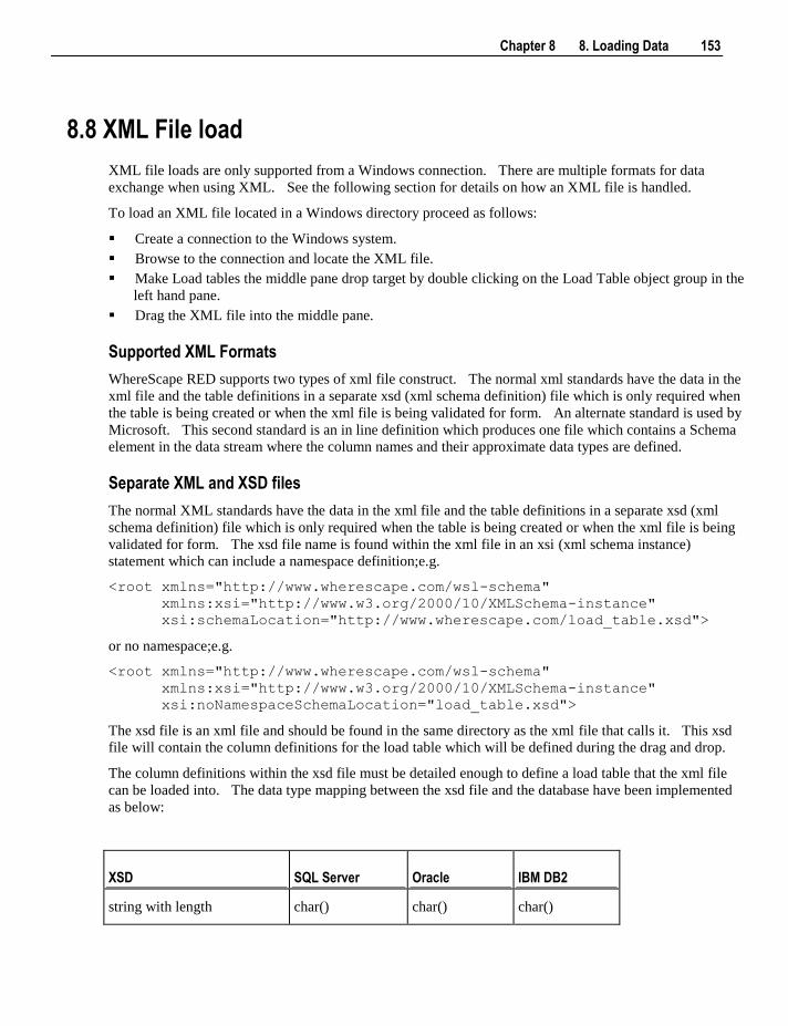
Chapter 8 8. Loading Data 153
8.8 XML File load
XML file loads are only supported from a Windows connection. There are multiple formats for data
exchange when using XML. See the following section for details on how an XML file is handled.
To load an XML file located in a Windows directory proceed as follows:
Create a connection to the Windows system.
Browse to the connection and locate the XML file.
Make Load tables the middle pane drop target by double clicking on the Load Table object group in the
left hand pane.
Drag the XML file into the middle pane.
Supported XML Formats
WhereScape RED supports two types of xml file construct. The normal xml standards have the data in the
xml file and the table definitions in a separate xsd (xml schema definition) file which is only required when
the table is being created or when the xml file is being validated for form. An alternate standard is used by
Microsoft. This second standard is an in line definition which produces one file which contains a Schema
element in the data stream where the column names and their approximate data types are defined.
Separate XML and XSD files
The normal XML standards have the data in the xml file and the table definitions in a separate xsd (xml
schema definition) file which is only required when the table is being created or when the xml file is being
validated for form. The xsd file name is found within the xml file in an xsi (xml schema instance)
statement which can include a namespace definition;e.g.
<root xmlns="http://www.wherescape.com/wsl-schema"
xmlns:xsi="http://www.w3.org/2000/10/XMLSchema-instance"
xsi:schemaLocation="http://www.wherescape.com/load_table.xsd">
or no namespace;e.g.
<root xmlns="http://www.wherescape.com/wsl-schema"
xmlns:xsi="http://www.w3.org/2000/10/XMLSchema-instance"
xsi:noNamespaceSchemaLocation="load_table.xsd">
The xsd file is an xml file and should be found in the same directory as the xml file that calls it. This xsd
file will contain the column definitions for the load table which will be defined during the drag and drop.
The column definitions within the xsd file must be detailed enough to define a load table that the xml file
can be loaded into. The data type mapping between the xsd file and the database have been implemented
as below:
XSD SQL Server Oracle IBM DB2
string with length char() char() char()
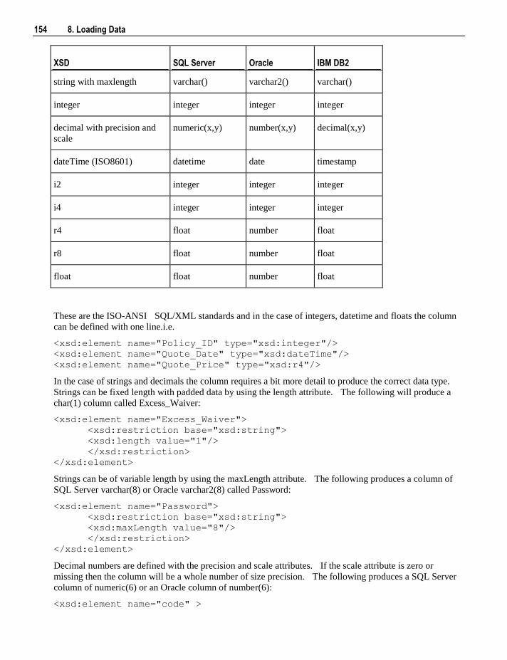
154 8. Loading Data
XSD SQL Server Oracle IBM DB2
string with maxlength varchar() varchar2() varchar()
integer integer integer integer
decimal with precision and
scale
numeric(x,y) number(x,y) decimal(x,y)
dateTime (ISO8601) datetime date timestamp
i2 integer integer integer
i4 integer integer integer
r4 float number float
r8 float number float
float float number float
These are the ISO-ANSI SQL/XML standards and in the case of integers, datetime and floats the column
can be defined with one line.i.e.
<xsd:element name="Policy_ID" type="xsd:integer"/>
<xsd:element name="Quote_Date" type="xsd:dateTime"/>
<xsd:element name="Quote_Price" type="xsd:r4"/>
In the case of strings and decimals the column requires a bit more detail to produce the correct data type.
Strings can be fixed length with padded data by using the length attribute. The following will produce a
char(1) column called Excess_Waiver:
<xsd:element name="Excess_Waiver">
<xsd:restriction base="xsd:string">
<xsd:length value="1"/>
</xsd:restriction>
</xsd:element>
Strings can be of variable length by using the maxLength attribute. The following produces a column of
SQL Server varchar(8) or Oracle varchar2(8) called Password:
<xsd:element name="Password">
<xsd:restriction base="xsd:string">
<xsd:maxLength value="8"/>
</xsd:restriction>
</xsd:element>
Decimal numbers are defined with the precision and scale attributes. If the scale attribute is zero or
missing then the column will be a whole number of size precision. The following produces a SQL Server
column of numeric(6) or an Oracle column of number(6):
<xsd:element name="code" >
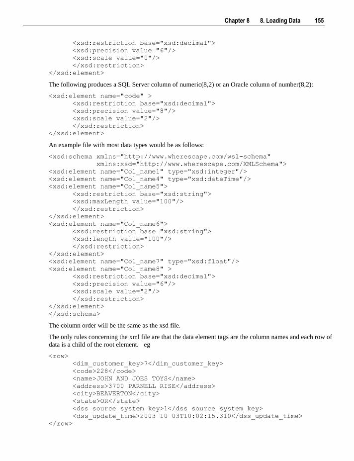
Chapter 8 8. Loading Data 155
<xsd:restriction base="xsd:decimal">
<xsd:precision value="6"/>
<xsd:scale value="0"/>
</xsd:restriction>
</xsd:element>
The following produces a SQL Server column of numeric(8,2) or an Oracle column of number(8,2):
<xsd:element name="code" >
<xsd:restriction base="xsd:decimal">
<xsd:precision value="8"/>
<xsd:scale value="2"/>
</xsd:restriction>
</xsd:element>
An example file with most data types would be as follows:
<xsd:schema xmlns="http://www.wherescape.com/wsl-schema"
xmlns:xsd="http://www.wherescape.com/XMLSchema">
<xsd:element name="Col_name1" type="xsd:integer"/>
<xsd:element name="Col_name4" type="xsd:dateTime"/>
<xsd:element name="Col_name5">
<xsd:restriction base="xsd:string">
<xsd:maxLength value="100"/>
</xsd:restriction>
</xsd:element>
<xsd:element name="Col_name6">
<xsd:restriction base="xsd:string">
<xsd:length value="100"/>
</xsd:restriction>
</xsd:element>
<xsd:element name="Col_name7" type="xsd:float"/>
<xsd:element name="Col_name8" >
<xsd:restriction base="xsd:decimal">
<xsd:precision value="6"/>
<xsd:scale value="2"/>
</xsd:restriction>
</xsd:element>
</xsd:schema>
The column order will be the same as the xsd file.
The only rules concerning the xml file are that the data element tags are the column names and each row of
data is a child of the root element. eg
<row>
<dim_customer_key>7</dim_customer_key>
<code>228</code>
<name>JOHN AND JOES TOYS</name>
<address>3700 PARNELL RISE</address>
<city>BEAVERTON</city>
<state>OR</state>
<dss_source_system_key>1</dss_source_system_key>
<dss_update_time>2003-10-03T10:02:15.310</dss_update_time>
</row>
156 8. Loading Data
Any columns which are missing from the row will be NULL in the loaded row.
The dateTime format in the xml file is defined as ISO8601 which looks like this:
2003-10-03T10:02:15.310
WhereScape RED will load this string into Oracle as:
TO_DATE(‘20031003100215’,’YYYYMMDDHH24MI’)
or for SQL Server:
CONVERT(DATETIME,‘2003-10-03T10:02:15.310’,126)
or for DB2:
TIMESTAMP_FORMAT('20031003100215', 'YYYYMMDDHH24MISS')
The xsd file is only required to create the load table, if the load table is only being loaded then this file is
ignored. To check that the xml and xsd files are well formed you can open them with any web browser.
If the files display with no errors then they are valid xml files.
In line schema definition
The other supported xml construct allows the use of in line schema definitions as produced by the Microsoft
FOR XML AUTO, ELEMENTS, XMLDATA query. This will produce one file which contains a Schema
element in which the column names and their approximate data types are defined. Because the supplied
data types are not concise enough to define the table columns correctly, this method will produce load
tables of either data type text for SQL Server or varchar2(4000) for Oracle. The column names are taken
from the <element type=”col_name”/> strings within the Schema element. The data elements will be the
same as above with the column names making up the start and end tags and the rows being the children of
the root element. The file that is produced by the FOR XML query above needs to be changed slightly to
comply with the xml standard. Remove everything before the Schema element and then give the file a
starting root element and a closing root element.eg <root> and </root>
The xml files can optionally start with an xml pre process statement.eg
<?xml version=”1.0”?>
They may also contain xml comments.eg
<!— comments -->
8.9 External Load
For an externally loaded table the only property that is executed is the Post Load procedure.
Any 'After' transformations recorded against any of the columns in an Externally loaded table will also be
processed.
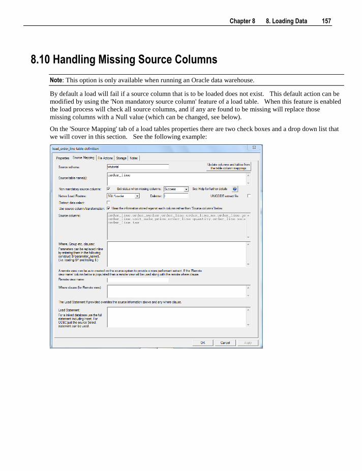
Chapter 8 8. Loading Data 157
8.10 Handling Missing Source Columns
Note: This option is only available when running an Oracle data warehouse.
By default a load will fail if a source column that is to be loaded does not exist. This default action can be
modified by using the 'Non mandatory source column' feature of a load table. When this feature is enabled
the load process will check all source columns, and if any are found to be missing will replace those
missing columns with a Null value (which can be changed, see below).
On the 'Source Mapping' tab of a load tables properties there are two check boxes and a drop down list that
we will cover in this section. See the following example:
158 8. Loading Data
Use Source column/transformation
When this check box is checked the 'Source columns' edit window is disabled. By default, and with this
box unchecked, a load table uses the contents of the 'Source columns' to specify which columns are being
extracted during a table load.
When this box is checked the load process builds up the statement to select from the source table(s) by
looking at the two fields source table and source column and any transformations associated with each
column in the load table. If a transformation is present then the transformation overrides the contents of
source table/source column. See the following section for more information on transformations.
Note: This box must be checked to enable non mandatory source column support.
Non mandatory source columns
When this check box is checked the load process will examine every column in the load table. Based on
the source table/source column fields associated with each column it will check to see if the column exists
in the source database. If the column exists normal processing will occur. If the column does not exist
then a Null will be substituted for the column, and the load will proceed.
If one or more columns are found to be missing the load process reports this situation. The status level of
this reporting can be set via the 'Exit status' drop down. See the following topic. In all cases the load will
be deemed to have been successful provided that no other errors occur.
Often Null values are not desirable in a data warehouse. This Null value can be replaced by some other
value by means of a 'During' or 'After' transformation. For example, a 'During' transformation, as shown
below, set on a missing column called 'State' will replace the Null with the value 'N/A'.
NVL(state,'N/A')
Exit status when missing columns
If columns are found to be missing as a result of a 'Non mandatory' check then a message is recorded in the
Audit trail and against the task if running in the Scheduler. The drop down list of the same name allows
the choice of action in the event of a missing column or columns. The choices are:
Choice Impact
Success The message informing that columns are missing uses an information status.
Warning The message issued is a warning. The table load will be identified as
successful but with warnings.
Error The message issued is an error. The table load will still complete successfully
albeit with an error message.
Chapter 8 8. Loading Data 159
This drop list is only available if the 'Non mandatory source columns' check box is checked.
Limitations of Missing Column check
The check for missing columns will only examine and check those columns that are recorded in the source
table and source column fields of a load table's column properties. Therefore if a source column is used in
a transformation or join, but is not recorded in the two fields mentioned above it will not be checked.
If a column is used in a transformation, it should have the same usage (name and case) as is found in the
source column and source table fields.
This check has no upper limit on the number of missing columns. All columns can be missing and the load
will still succeed.
8.11 Load Table Transformations
Each load table column can have a transformation associated with it. See Transformations (see "19.
Transformations" on page 387) and Load Table Column Transformations (see "19.1.2 Load Table
Column Transformations" on page 390) for more details.
8.11.1 Post-Load Procedures If a procedure name is entered in the post-load procedure field of a load table's properties, then this
procedure will be executed after the load has completed and after any 'after' transformations have occurred.
8.12 Changing Load Connection and Schema
The connection associated with a load table can be changed through the properties of that table.
Connections can also be changed in bulk by using the following process:
1 Double click on the 'Load Tables' object group in the left pane. This will display all load tables in the
middle pane.
2 Select those load tables that you wish to change using standard Windows selection.
3 Right mouse to bring up a menu and select 'Change Connect/Schema'.
4 Select the new connection to change all the selected load tables.
160 8. Loading Data
Note: You cannot change the connection type but it is possible to change from Database to ODBC
connections when the following considerations are taken into account.
Switching Connection from ODBC to Database
This switch should be successful in most cases, although it may not provide the most performant load
possible. By default ODBC connections use the source table / column transformation loading method as
dates and potentially other data types need to be converted.
When switching to a database link load any transformations will still occur although they may no longer be
necessary.
Switching Connection from Database to ODBC
Although it is possible to switch from a Database connection to an ODBC connection, the resultant extract
may not function correctly. The main issue is around the conversion of date fields under Oracle. SQL
Server tends to handle the date conversion better in most cases. When an extract occurs over an ODBC
connection the date is converted in the extract from the source system into a standard ASCII format. This
ASCII formatted date is then converted back when it is loaded into the load table. To resolve this problem
place a transformation on any date fields. Examples of typical Oracle transformations are:
'to_date('''||to_char(ORDER_DATE,'YYYYMMDD')||''',''YYYYMMDD'')'
to_char(ORDER_DATE,'YYYY-MM-DD HH24:MI:SS')
where ORDER_DATE is the name of the column being extracted. In the first example the conversion
string is enclosed within quote marks (') so that it is passed as a literal to the select statement that will be
built. Quote marks within the conversion string are protected from premature evaluation by the inclusion
of a second quote mark alongside the original.
Note: If a load table is created via drag and drop from an ODBC based connection WhereScape RED will
build all the required date transformations.
There are several supplied APIs for changing schema and connections programmatically. See Callable
Procedures (see "29. Callable Procedures" on page 565) for more details.
Chapter 9 9. Dimensions 161
In This Chapter
9.1 Dimensions Overview ........................................................... 162
9.2 Building a Dimension ........................................................... 164
9.3 Generating the Dimension Update Procedure ....................... 171
9.4 Dimension Artificial Keys .................................................... 179
9.5 Dimension Get Key Function................................................ 180
9.6 Dimension Initial Build ......................................................... 181
9.7 Dimension Column Properties .............................................. 182
9.8 Dimension Column Transformations .................................... 189
9.9 Dimension Hierarchies .......................................................... 189
9.10 Snowflake ........................................................................... 191
9.11 Dimension Language Mapping ........................................... 193
C H A P T E R 9
9. Dimensions
162 9. Dimensions
9.1 Dimensions Overview
A dimension table is normally defined, for our purposes, as a table that allows us to constrain queries on the
fact table.
A dimension is built from the Data Warehouse connection. Unless you are doing a retro-fit of an existing
system, dimensions are typically built from one or more load tables.
The normal steps for creating a dimension are defined below and are covered in this chapter. The steps
are:
Identify the source transactional data that will constitute the dimension. If the data is sourced from
multiple tables ascertain if a join between the source tables is possible, or if a series of lookups would
be a better option.
Using the 'drag and drop' functionality drag the load table that is the primary source of information for
the dimension into a dimension target. See Building a Dimension (see "9.2 Building a Dimension"
on page 164).
If only one table is being sourced and most of the columns are to be used (or if prototyping) you can
select the auto create option to build and load the dimension and skip the next 4 steps. See Building a
Dimension (see "9.2 Building a Dimension" on page 164).
Add columns from other load tables if required. See Building a Dimension (see "9.2 Building a
Dimension" on page 164).
Create the dimension table in the database. See Building a Dimension (see "9.2 Building a
Dimension" on page 164).
Build the update procedure. See Generating the Dimension Update Procedure (see "9.3 Generating
the Dimension Update Procedure" on page 171).
Run the update procedure and analyze the results. See Dimension Initial Build (see "9.6 Dimension
Initial Build" on page 181).
Modify the update procedure as required. See Dimension Initial Build (see "9.6 Dimension Initial Build"
on page 181).
Dimension Keys
Dimensions have two types of keys that we will refer to frequently. These are the Business Key and the
Artificial Key. A definition of these two key types follows:
Business Key
The business key is the column or columns that uniquely identify a record within the dimension. Where
the dimension maps back to a single or a main table in the source system, it is usually possible to ascertain
the business key by looking at the unique keys for that source table. Some people refer to the business key
as the 'natural' key. Examples of business keys are:
The product SKU in a product dimension
The customer code in a customer dimension
The calendar date in a date dimension
The 24 hour time in a time dimension (i.e. HHMM) (e.g. 1710)
The airport short code in an airport dimension.
Chapter 9 9. Dimensions 163
It is assumed that business keys will never be NULL. If a null value is possible in a business key then the
generated code will need to be modified to handle the null value by assigning some default value. For
example the Where clause in a dimension update may become:
SQL Server: Where isnull(business_key,'N/A') = isnull(v_LoadRec.business_key,'N/A')
Oracle: Where nvl(business_key,'N/A') = nvl(v_LoadRec.business_key,'N/A')
DB2: Where coalesce(business_key,'N/A') = coalesce(v_LoadRec.business_key,'N/A')
Note: Business keys are assumed to never be Null. If they could be null it is best to transform them to
some value prior to dimension or stage table update. If this is not done an unmodified update will probably
fail with a duplicate key error on the business key index.
Artificial Key
The artificial key is the unique identifier that is used to join a dimension record to a fact table. When
joining dimensions to fact tables it would be possible to perform the join using the business key. For fact
tables with a large number of records this however would result in slow query times and very large indexes.
As query time is one of our key drivers in data warehouse implementations the best answer is always to use
some form of artificial key. A price is paid in the additional processing required to build the fact table
rows, but this is offset by the reduced query times and index sizes. We can also make use of database
specific features such as bitmap indexes in Oracle.
The artificial key is an integer and is built sequentially from 1 upwards. See the section on artificial keys
for a more detailed explanation. An artificial key is sometimes referred to as a "surrogate" key.
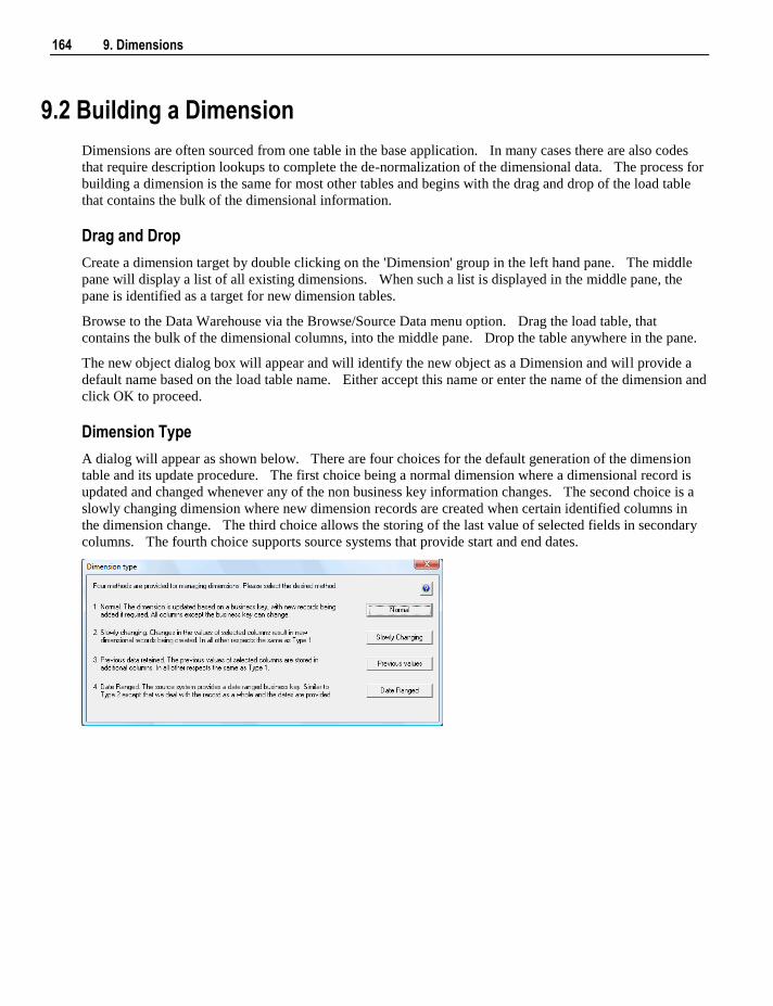
164 9. Dimensions
9.2 Building a Dimension
Dimensions are often sourced from one table in the base application. In many cases there are also codes
that require description lookups to complete the de-normalization of the dimensional data. The process for
building a dimension is the same for most other tables and begins with the drag and drop of the load table
that contains the bulk of the dimensional information.
Drag and Drop
Create a dimension target by double clicking on the 'Dimension' group in the left hand pane. The middle
pane will display a list of all existing dimensions. When such a list is displayed in the middle pane, the
pane is identified as a target for new dimension tables.
Browse to the Data Warehouse via the Browse/Source Data menu option. Drag the load table, that
contains the bulk of the dimensional columns, into the middle pane. Drop the table anywhere in the pane.
The new object dialog box will appear and will identify the new object as a Dimension and will provide a
default name based on the load table name. Either accept this name or enter the name of the dimension and
click OK to proceed.
Dimension Type
A dialog will appear as shown below. There are four choices for the default generation of the dimension
table and its update procedure. The first choice being a normal dimension where a dimensional record is
updated and changed whenever any of the non business key information changes. The second choice is a
slowly changing dimension where new dimension records are created when certain identified columns in
the dimension change. The third choice allows the storing of the last value of selected fields in secondary
columns. The fourth choice supports source systems that provide start and end dates.
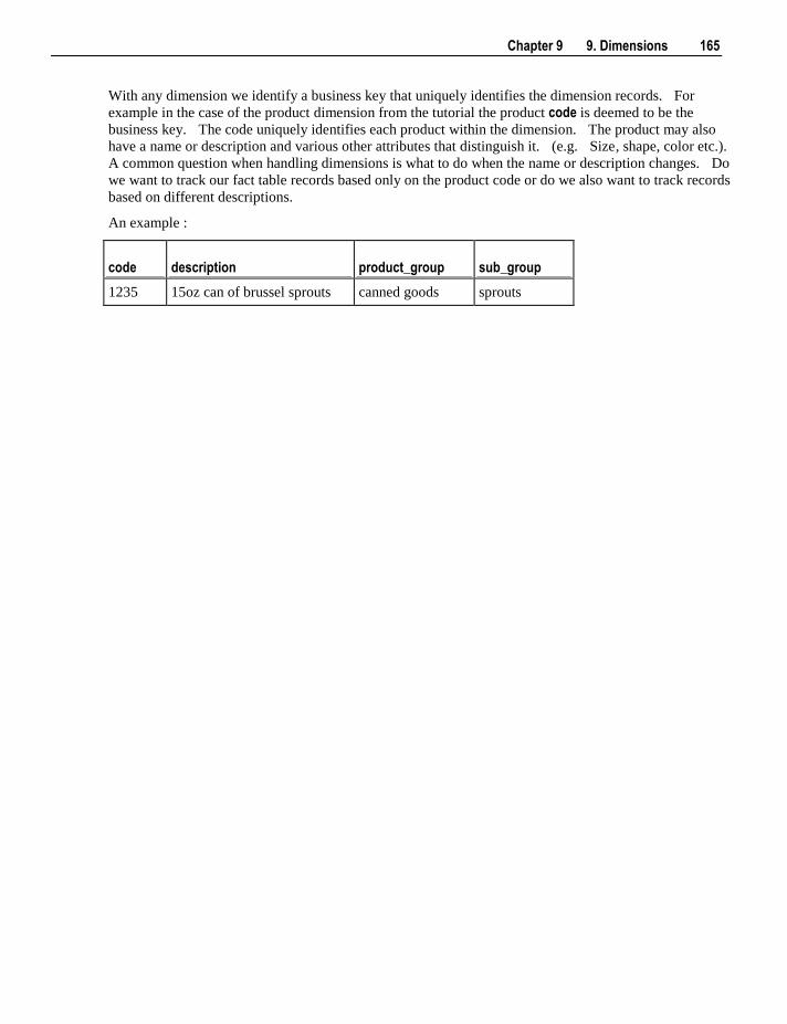
Chapter 9 9. Dimensions 165
With any dimension we identify a business key that uniquely identifies the dimension records. For
example in the case of the product dimension from the tutorial the product code is deemed to be the
business key. The code uniquely identifies each product within the dimension. The product may also
have a name or description and various other attributes that distinguish it. (e.g. Size, shape, color etc.).
A common question when handling dimensions is what to do when the name or description changes. Do
we want to track our fact table records based only on the product code or do we also want to track records
based on different descriptions.
An example :
code description product_group sub_group
1235 15oz can of brussel sprouts canned goods sprouts
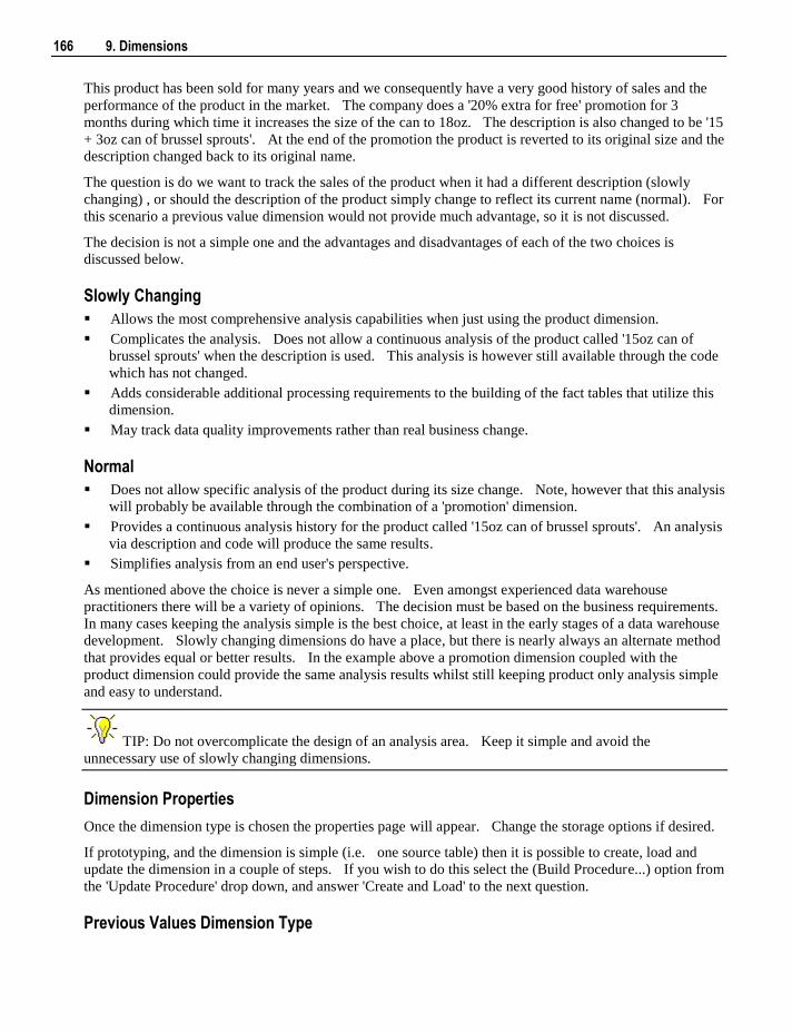
166 9. Dimensions
This product has been sold for many years and we consequently have a very good history of sales and the
performance of the product in the market. The company does a '20% extra for free' promotion for 3
months during which time it increases the size of the can to 18oz. The description is also changed to be '15
+ 3oz can of brussel sprouts'. At the end of the promotion the product is reverted to its original size and the
description changed back to its original name.
The question is do we want to track the sales of the product when it had a different description (slowly
changing) , or should the description of the product simply change to reflect its current name (normal). For
this scenario a previous value dimension would not provide much advantage, so it is not discussed.
The decision is not a simple one and the advantages and disadvantages of each of the two choices is
discussed below.
Slowly Changing
Allows the most comprehensive analysis capabilities when just using the product dimension.
Complicates the analysis. Does not allow a continuous analysis of the product called '15oz can of
brussel sprouts' when the description is used. This analysis is however still available through the code
which has not changed.
Adds considerable additional processing requirements to the building of the fact tables that utilize this
dimension.
May track data quality improvements rather than real business change.
Normal
Does not allow specific analysis of the product during its size change. Note, however that this analysis
will probably be available through the combination of a 'promotion' dimension.
Provides a continuous analysis history for the product called '15oz can of brussel sprouts'. An analysis
via description and code will produce the same results.
Simplifies analysis from an end user's perspective.
As mentioned above the choice is never a simple one. Even amongst experienced data warehouse
practitioners there will be a variety of opinions. The decision must be based on the business requirements.
In many cases keeping the analysis simple is the best choice, at least in the early stages of a data warehouse
development. Slowly changing dimensions do have a place, but there is nearly always an alternate method
that provides equal or better results. In the example above a promotion dimension coupled with the
product dimension could provide the same analysis results whilst still keeping product only analysis simple
and easy to understand.
TIP: Do not overcomplicate the design of an analysis area. Keep it simple and avoid the
unnecessary use of slowly changing dimensions.
Dimension Properties
Once the dimension type is chosen the properties page will appear. Change the storage options if desired.
If prototyping, and the dimension is simple (i.e. one source table) then it is possible to create, load and
update the dimension in a couple of steps. If you wish to do this select the (Build Procedure...) option from
the 'Update Procedure' drop down, and answer 'Create and Load' to the next question.
Previous Values Dimension Type
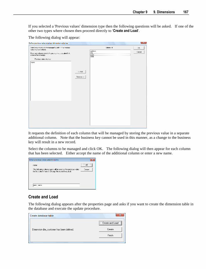
Chapter 9 9. Dimensions 167
If you selected a 'Previous values' dimension type then the following questions will be asked. If one of the
other two types where chosen then proceed directly to 'Create and Load'.
The following dialog will appear:
It requests the definition of each column that will be managed by storing the previous value in a separate
additional column. Note that the business key cannot be used in this manner, as a change to the business
key will result in a new record.
Select the columns to be managed and click OK. The following dialog will then appear for each column
that has been selected. Either accept the name of the additional column or enter a new name.
Create and Load
The following dialog appears after the properties page and asks if you want to create the dimension table in
the database and execute the update procedure.
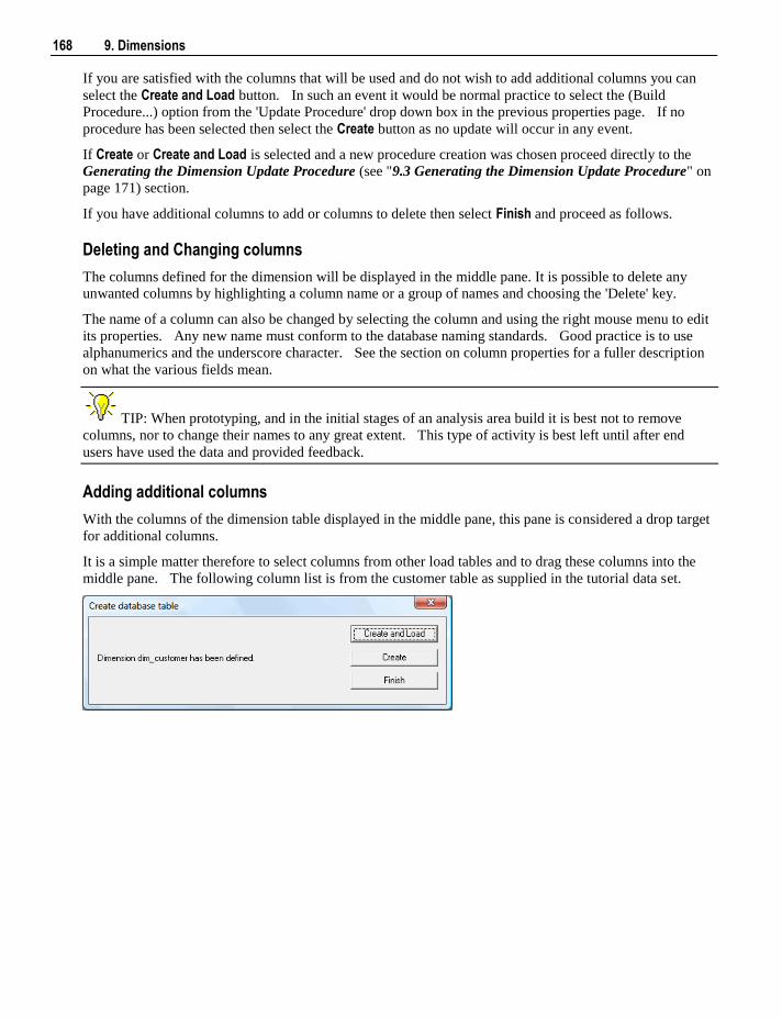
168 9. Dimensions
If you are satisfied with the columns that will be used and do not wish to add additional columns you can
select the Create and Load button. In such an event it would be normal practice to select the (Build
Procedure...) option from the 'Update Procedure' drop down box in the previous properties page. If no
procedure has been selected then select the Create button as no update will occur in any event.
If Create or Create and Load is selected and a new procedure creation was chosen proceed directly to the
Generating the Dimension Update Procedure (see "9.3 Generating the Dimension Update Procedure" on
page 171) section.
If you have additional columns to add or columns to delete then select Finish and proceed as follows.
Deleting and Changing columns
The columns defined for the dimension will be displayed in the middle pane. It is possible to delete any
unwanted columns by highlighting a column name or a group of names and choosing the 'Delete' key.
The name of a column can also be changed by selecting the column and using the right mouse menu to edit
its properties. Any new name must conform to the database naming standards. Good practice is to use
alphanumerics and the underscore character. See the section on column properties for a fuller description
on what the various fields mean.
TIP: When prototyping, and in the initial stages of an analysis area build it is best not to remove
columns, nor to change their names to any great extent. This type of activity is best left until after end
users have used the data and provided feedback.
Adding additional columns
With the columns of the dimension table displayed in the middle pane, this pane is considered a drop target
for additional columns.
It is a simple matter therefore to select columns from other load tables and to drag these columns into the
middle pane. The following column list is from the customer table as supplied in the tutorial data set.
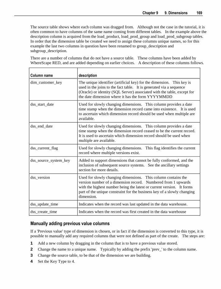
Chapter 9 9. Dimensions 169
The source table shows where each column was dragged from. Although not the case in the tutorial, it is
often common to have columns of the same name coming from different tables. In the example above the
description column is acquired from the load_product, load_prod_group and load_prod_subgroup tables.
In order that the dimension table be created we need to assign these columns unique names, so for this
example the last two columns in question have been renamed to group_description and
subgroup_description.
There are a number of columns that do not have a source table. These columns have been added by
WhereScape RED, and are added depending on earlier choices. A description of these columns follows.
Column name description
dim_customer_key The unique identifier (artificial key) for the dimension. This key is
used in the joins to the fact table. It is generated via a sequence
(Oracle) or identity (SQL Server) associated with the table, except for
the date dimension where it has the form YYYYMMDD
dss_start_date Used for slowly changing dimensions. This column provides a date
time stamp when the dimension record came into existence. It is used
to ascertain which dimension record should be used when multiple are
available.
dss_end_date Used for slowly changing dimensions. This column provides a date
time stamp when the dimension record ceased to be the current record.
It is used to ascertain which dimension record should be used when
multiple are available.
dss_current_flag Used for slowly changing dimensions. This flag identifies the current
record where multiple versions exist.
dss_source_system_key Added to support dimensions that cannot be fully conformed, and the
inclusion of subsequent source systems. See the ancillary settings
section for more details.
dss_version Used for slowly changing dimensions. This column contains the
version number of a dimension record. Numbered from 1 upwards
with the highest number being the latest or current version. It forms
part of the unique constraint for the business key of a slowly changing
dimension.
dss_update_time Indicates when the record was last updated in the data warehouse.
dss_create_time Indicates when the record was first created in the data warehouse
Manually adding previous value columns
If a 'Previous value' type of dimension is chosen, or in fact if the dimension is converted to this type, it is
possible to manually add any required columns that were not defined as part of the create. The steps are:
1 Add a new column by dragging in the column that is to have a previous value stored.
2 Change the name to a unique name. Typically by adding the prefix 'prev_' to the column name.
3 Change the source table, to be that of the dimension we are building.
4 Set the Key Type to 4.
170 9. Dimensions
Having performed these actions WhereScape RED will detect the column and build the appropriate code
during the procedure generation phase.
Create the table
Once the dimension has been defined in the metadata we need to physically create the table in the database.
This is achieved by using the right mouse button when positioned over the dimension name and selecting
Create (ReCreate) from the popup menu.
A results dialog box will appear to show the results of the creation.
The contents of this dialog are a message to the effect that the dimension table was created. A copy of the
actual database create statement, the sequence create statement (Oracle only), and if defined the results of
any index create statements will be listed. For the initial create no indexes will be defined.
If the table was not created then ascertain and fix the problem. A common problem is 'Duplicate column'
where a column has the same name in two of the source tables. The best way of finding such a column is
to double click on the list heading 'Col name'. This will sort the column names into alphabetic order.
Another double click on the heading will sort the columns back into their create order.
For Oracle data warehouses the sequence created as part of the table create is normally called
table_name_seq unless the default has been overridden. If this sequence already exists a warning is issued.
This sequence is used in the assigning of a unique artificial key to the dimension. SQL Server makes use
of an identity attribute on the artificial key column.
The next section covers the Generating the Dimension Update Procedure (see "9.3 Generating the
Dimension Update Procedure" on page 171).
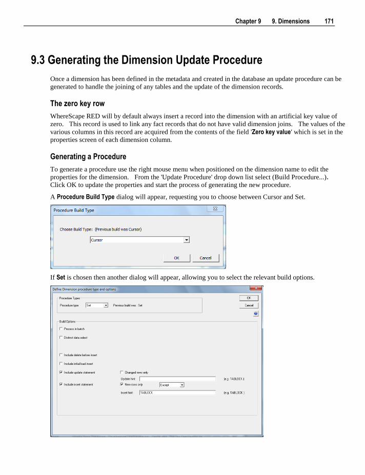
Chapter 9 9. Dimensions 171
9.3 Generating the Dimension Update Procedure
Once a dimension has been defined in the metadata and created in the database an update procedure can be
generated to handle the joining of any tables and the update of the dimension records.
The zero key row
WhereScape RED will by default always insert a record into the dimension with an artificial key value of
zero. This record is used to link any fact records that do not have valid dimension joins. The values of the
various columns in this record are acquired from the contents of the field 'Zero key value' which is set in the
properties screen of each dimension column.
Generating a Procedure
To generate a procedure use the right mouse menu when positioned on the dimension name to edit the
properties for the dimension. From the 'Update Procedure' drop down list select (Build Procedure...). Click OK to update the properties and start the process of generating the new procedure.
A Procedure Build Type dialog will appear, requesting you to choose between Cursor and Set.
If Set is chosen then another dialog will appear, allowing you to select the relevant build options.
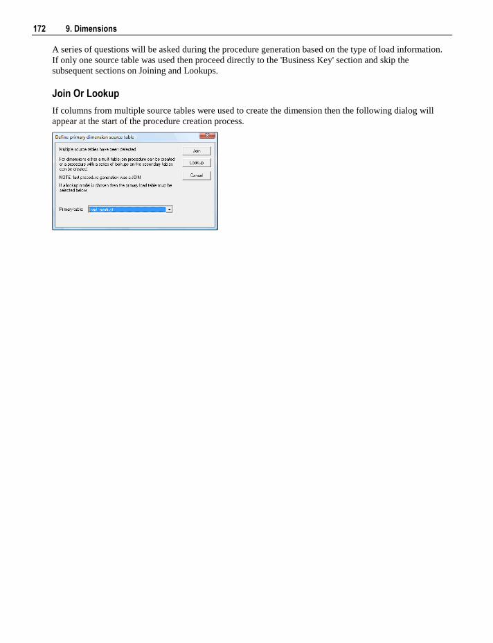
172 9. Dimensions
A series of questions will be asked during the procedure generation based on the type of load information.
If only one source table was used then proceed directly to the 'Business Key' section and skip the
subsequent sections on Joining and Lookups.
Join Or Lookup
If columns from multiple source tables were used to create the dimension then the following dialog will
appear at the start of the procedure creation process.
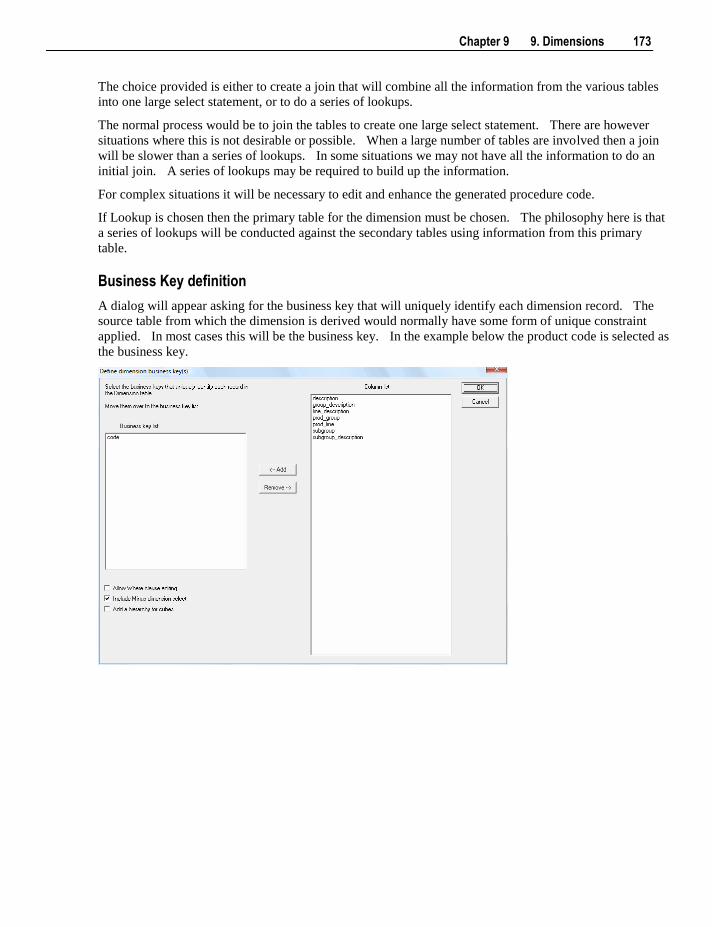
Chapter 9 9. Dimensions 173
The choice provided is either to create a join that will combine all the information from the various tables
into one large select statement, or to do a series of lookups.
The normal process would be to join the tables to create one large select statement. There are however
situations where this is not desirable or possible. When a large number of tables are involved then a join
will be slower than a series of lookups. In some situations we may not have all the information to do an
initial join. A series of lookups may be required to build up the information.
For complex situations it will be necessary to edit and enhance the generated procedure code.
If Lookup is chosen then the primary table for the dimension must be chosen. The philosophy here is that
a series of lookups will be conducted against the secondary tables using information from this primary
table.
Business Key definition
A dialog will appear asking for the business key that will uniquely identify each dimension record. The
source table from which the dimension is derived would normally have some form of unique constraint
applied. In most cases this will be the business key. In the example below the product code is selected as
the business key.
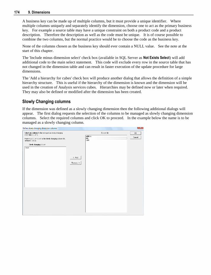
174 9. Dimensions
A business key can be made up of multiple columns, but it must provide a unique identifier. Where
multiple columns uniquely and separately identify the dimension, choose one to act as the primary business
key. For example a source table may have a unique constraint on both a product code and a product
description. Therefore the description as well as the code must be unique. It is of course possible to
combine the two columns, but the normal practice would be to choose the code as the business key.
None of the columns chosen as the business key should ever contain a NULL value. See the note at the
start of this chapter.
The 'Include minus dimension select' check box (available in SQL Server as Not Exists Select) will add
additional code to the main select statement. This code will exclude every row in the source table that has
not changed in the dimension table and can result in faster execution of the update procedure for large
dimensions.
The 'Add a hierarchy for cubes' check box will produce another dialog that allows the definition of a simple
hierarchy structure. This is useful if the hierarchy of the dimension is known and the dimension will be
used in the creation of Analysis services cubes. Hierarchies may be defined now or later when required.
They may also be defined or modified after the dimension has been created.
Slowly Changing columns
If the dimension was defined as a slowly changing dimension then the following additional dialogs will
appear. The first dialog requests the selection of the columns to be managed as slowly changing dimension
columns. Select the required columns and click OK to proceed. In the example below the name is to be
managed as a slowly changing column.
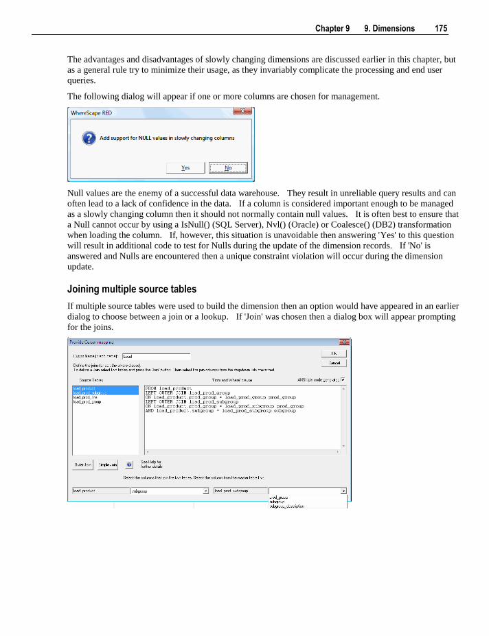
Chapter 9 9. Dimensions 175
The advantages and disadvantages of slowly changing dimensions are discussed earlier in this chapter, but
as a general rule try to minimize their usage, as they invariably complicate the processing and end user
queries.
The following dialog will appear if one or more columns are chosen for management.
Null values are the enemy of a successful data warehouse. They result in unreliable query results and can
often lead to a lack of confidence in the data. If a column is considered important enough to be managed
as a slowly changing column then it should not normally contain null values. It is often best to ensure that
a Null cannot occur by using a IsNull() (SQL Server), Nvl() (Oracle) or Coalesce() (DB2) transformation
when loading the column. If, however, this situation is unavoidable then answering 'Yes' to this question
will result in additional code to test for Nulls during the update of the dimension records. If 'No' is
answered and Nulls are encountered then a unique constraint violation will occur during the dimension
update.
Joining multiple source tables
If multiple source tables were used to build the dimension then an option would have appeared in an earlier
dialog to choose between a join or a lookup. If 'Join' was chosen then a dialog box will appear prompting
for the joins.
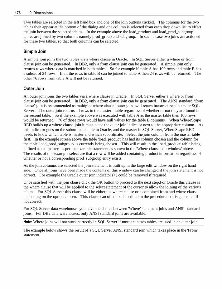
176 9. Dimensions
Two tables are selected in the left hand box and one of the join buttons clicked. The columns for the two
tables then appear at the bottom of the dialog and one column is selected from each drop down list to effect
the join between the selected tables. In the example above the load_product and load_prod_subgroup
tables are joined by two columns namely prod_group and subgroup. In such a case two joins are actioned
for these two tables, so that both columns can be selected.
Simple Join
A simple join joins the two tables via a where clause in Oracle. In SQL Server either a where or from
clause join can be generated. In DB2, only a from clause join can be generated. A simple join only
returns rows where data is matched in both tables. So for example if table A has 100 rows and table B has
a subset of 24 rows. If all the rows in table B can be joined to table A then 24 rows will be returned. The
other 76 rows from table A will not be returned.
Outer Join
An outer join joins the two tables via a where clause in Oracle. In SQL Server either a where or from
clause join can be generated. In DB2, only a from clause join can be generated. The ANSI standard „from
clause‟ join is recommended as multiple „where clause‟ outer joins will return incorrect results under SQL
Server. The outer join returns all rows in the master table regardless of whether or not they are found in
the second table. So if the example above was executed with table A as the master table then 100 rows
would be returned. 76 of those rows would have null values for the table B columns. When WhereScape
RED builds up a where clause join it must place the outer join indicator next to the appropriate column. As
this indicator goes on the subordinate table in Oracle, and the master in SQL Server, WhereScape RED
needs to know which table is master and which subordinate. Select the join column from the master table
first. In the example screen above the table 'load_product' has had its column chosen and the column for
the table 'load_prod_subgroup' is currently being chosen. This will result in the 'load_product' table being
defined as the master, as per the example statement as shown in the 'Where clause edit window' above.
The results of this example select are that a row will be added containing product information regardless of
whether or not a corresponding prod_subgroup entry exists.
As the join columns are selected the join statement is built up in the large edit window on the right hand
side. Once all joins have been made the contents of this window can be changed if the join statement is not
correct. For example the Oracle outer join indicator (+) could be removed if required.
Once satisfied with the join clause click the OK button to proceed to the next step.For Oracle this clause is
the where clause that will be applied to the select statement of the cursor to allow the joining of the various
tables. For SQL Server this clause will be either the where clause or a combined from and where clause
depending on the option chosen. This clause can of course be edited in the procedure that is generated if
not correct.
For SQL Server data warehouses you have the choice between 'Where' statement joins and ANSI standard
joins. For DB2 data warehouses, only ANSI standard joins are available.
Note: Where joins will not work correctly in SQL Server if more than two tables are used in an outer join.
The example below shows the result of a SQL Server ANSI standard join which takes place in the 'From'
statement.
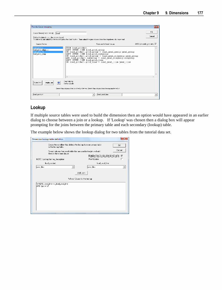
Chapter 9 9. Dimensions 177
Lookup
If multiple source tables were used to build the dimension then an option would have appeared in an earlier
dialog to choose between a join or a lookup. If 'Lookup' was chosen then a dialog box will appear
prompting for the joins between the primary table and each secondary (lookup) table.
The example below shows the lookup dialog for two tables from the tutorial data set.
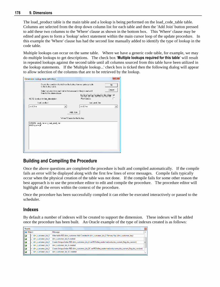
178 9. Dimensions
The load_product table is the main table and a lookup is being performed on the load_code_table table.
Columns are selected from the drop down column list for each table and then the 'Add Join' button pressed
to add these two columns to the 'Where' clause as shown in the bottom box. This 'Where' clause may be
edited and goes to form a 'lookup' select statement within the main cursor loop of the update procedure. In
this example the 'Where' clause has had the second line manually added to identify the type of lookup in the
code table.
Multiple lookups can occur on the same table. Where we have a generic code table, for example, we may
do multiple lookups to get descriptions. The check box 'Multiple lookups required for this table' will result
in repeated lookups against the second table until all columns sourced from this table have been utilized in
the lookup statements. If the 'Multiple lookup...' check box is ticked then the following dialog will appear
to allow selection of the columns that are to be retrieved by the lookup.
Building and Compiling the Procedure
Once the above questions are completed the procedure is built and compiled automatically. If the compile
fails an error will be displayed along with the first few lines of error messages. Compile fails typically
occur when the physical creation of the table was not done. If the compile fails for some other reason the
best approach is to use the procedure editor to edit and compile the procedure. The procedure editor will
highlight all the errors within the context of the procedure.
Once the procedure has been successfully compiled it can either be executed interactively or passed to the
scheduler.
Indexes
By default a number of indexes will be created to support the dimension. These indexes will be added
once the procedure has been built. An Oracle example of the type of indexes created is as follows:
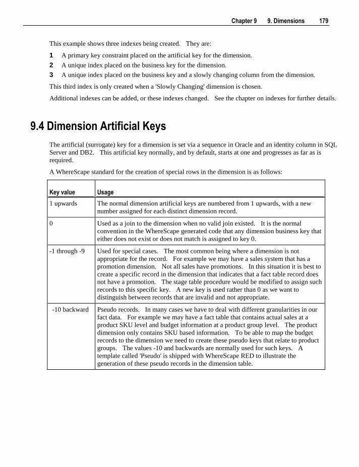
Chapter 9 9. Dimensions 179
This example shows three indexes being created. They are:
1 A primary key constraint placed on the artificial key for the dimension.
2 A unique index placed on the business key for the dimension.
3 A unique index placed on the business key and a slowly changing column from the dimension.
This third index is only created when a 'Slowly Changing' dimension is chosen.
Additional indexes can be added, or these indexes changed. See the chapter on indexes for further details.
9.4 Dimension Artificial Keys
The artificial (surrogate) key for a dimension is set via a sequence in Oracle and an identity column in SQL
Server and DB2. This artificial key normally, and by default, starts at one and progresses as far as is
required.
A WhereScape standard for the creation of special rows in the dimension is as follows:
Key value Usage
1 upwards The normal dimension artificial keys are numbered from 1 upwards, with a new
number assigned for each distinct dimension record.
0 Used as a join to the dimension when no valid join existed. It is the normal
convention in the WhereScape generated code that any dimension business key that
either does not exist or does not match is assigned to key 0.
-1 through -9 Used for special cases. The most common being where a dimension is not
appropriate for the record. For example we may have a sales system that has a
promotion dimension. Not all sales have promotions. In this situation it is best to
create a specific record in the dimension that indicates that a fact table record does
not have a promotion. The stage table procedure would be modified to assign such
records to this specific key. A new key is used rather than 0 as we want to
distinguish between records that are invalid and not appropriate.
-10 backward Pseudo records. In many cases we have to deal with different granularities in our
fact data. For example we may have a fact table that contains actual sales at a
product SKU level and budget information at a product group level. The product
dimension only contains SKU based information. To be able to map the budget
records to the dimension we need to create these pseudo keys that relate to product
groups. The values -10 and backwards are normally used for such keys. A
template called 'Pseudo' is shipped with WhereScape RED to illustrate the
generation of these pseudo records in the dimension table.
180 9. Dimensions
9.5 Dimension Get Key Function
When WhereScape RED is asked to generate a new procedure to support the updating of a dimension it also
generates a 'Get Key' function (procedure in SQL Server and DB2). Such a function is also generated
when dimension views are created, and can be generated for retro-fitted dimensions.
This 'Get Key' function is used to return an artificial key when supplied a business key. The normal syntax
is to call the function passing the business key and be returned a status indicating the result of the lookup.
On a successful lookup the artificial key for the dimension record is also returned. If the lookup fails
because the business key is not found in the dimension then an appropriate status is returned and the
artificial key is set to 0.
Note: Two parameters exist on the generated 'Get Key' function that allow manipulation of the process. It
is possible to automatically add a new dimension record when a match is not made. It is also possible to
record the lookup failure in the detail/error log. By default both these options are disabled.
Modifying the 'Get Key' function
There may be a situation where a dimension record can have multiple business keys.
For example: you may be able to look up a 'factory' based on the factory code, the name of the factory or its
address. The generated 'Get Key' function will only support the primary business key which in this case
may be the factory code. However, we may have a fact record that only contains the factory name. In
such a case we need to modify the 'Get Key' function or add a second function. The advantages of adding
a second function are that any code generated in the future that uses this dimension will work without
modification. The disadvantages are the multiple points of maintenance required when changing the
dimension. Both options are discussed below:
Adding a second 'Get Key' function for a dimension
Choose a name similar to the existing function. If say we have a 'get_dim_factory_key' function then we
may choose a name like 'get_factory_name_key'. Proceed to create and populate the function as follows:
1 Using the right mouse menu with the 'Procedure' group highlighted in the left pane, select the 'New Object' option to create a new procedure. Put the name chosen in the name field and click ADD.
2 A properties dialog will appear. Change the type to 'Function' for Oracle, leave as a 'Procedure' for
SQL Server. Enter a description under the 'Purpose' column and click the UPDATE button.
3 Expand the 'Procedure' group in the left pane and double click on the new object just created. This
will start the editor.
4 Select the Tools/View procedure or template menu option. This will start a dialog box.
5 Select the existing 'Get Key' function from the procedure drop down. A new window will appear on
the right hand side showing the existing 'Get Key' function.
6 Click the mouse in the existing function window. Using the right mouse menu choose 'Select All' and
then using the right mouse menu again choose 'Copy'.
7 Click the mouse in the main editor window and paste the existing function into the window. The
existing function window can now be closed if desired.
8 Using the menu option Edit/Replace change all occurrences of the old function name to the new name.
9 Change the various occurrences of the business key name and variable to match the new one and test it
all.
Chapter 9 9. Dimensions 181
Once a new 'Get Key' function has been produced it will obviously be necessary to modify the stage update
procedure to utilize the new function.
TIP: An alternative approach is to create a dimension view specifically to generate a different kind of
get key function. Then use this view's surrogate key in the stage table instead of the dimension table's
surrogate key. This approach avoids modifying the staging table procedure.
Extending the 'Get Key' function
If you want to keep all the information for the lookup of dimension keys in one location then extend the
functionality of the existing 'Get Key' function. The normal practice in this case is to include all potential
business keys as parameters. Multiple select statements can be employed to select the keys based on the
appropriate business key. To choose the correct statement either use Nulls in the unused business keys or
include an additional parameter to indicate which business key is being passed.
If this method is used then any stage update procedures will need to be modified to handle the new calling
syntax.
9.6 Dimension Initial Build
The initial population of a dimension with data can be achieved by generating a custom procedure and then;
using the right mouse on the dimension, choosing Execute Custom Procedure via Scheduler. The dimension
should be analyzed once the custom procedure is completed so that the database query optimizer can make
use of the indexes.
For smaller dimensions (i.e. less than 500,000 rows) run the normal 'Update' procedure against an empty
dimension table. There is however a danger in this action in that the query optimizer will not have any
information on the table and hence will do a full table pass when adding each new row. For a very small
dimension this will not be an issue, but it will rapidly become a major problem as the row count increases.
The problem with the initial update is that the database does not know to use the index that has been created
for the business key, and hence does a full table pass when attempting to update/insert a record.
To prevent this problem the generated code will issue an analyze statement after 1000 rows have been
added to the table. The statement used is as follows:
SQL Server: update statistics dim_table with sample 5 percent
Oracle: analyze table dim_table estimate statistics sample 5 percent for all indexed columns
DB2: runstats on table dim_table
where dim_table is the name of the dimension.
This command will be issued whenever 1000 or more new rows are added to a dimension. If this is
undesirable then the code should be removed from the update procedure. It may be undesirable if a plan
has been locked in for the table.
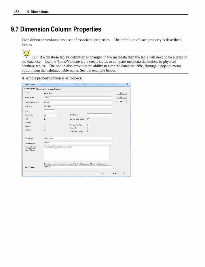
182 9. Dimensions
9.7 Dimension Column Properties
Each dimension column has a set of associated properties. The definition of each property is described
below:
TIP: If a database table's definition is changed in the metadata then the table will need to be altered in
the database. Use the Tools/Validate table create status to compare metadata definitions to physical
database tables. The option also provides the ability to alter the database table, through a pop-up menu
option from the validated table name. See the example below.
A sample property screen is as follows:
Chapter 9 9. Dimensions 183
The two special update keys allow you to update the column and step either forward or backward to the
next column's properties. ALT-Left Arrow and ALT-Right Arrow can also be used instead of the two special
update keys.
Table
The table to which the column belongs. Read only.
Column name
The database name of the column. This name must conform to database column naming standards.
Typically such standards exclude the use of spaces etc. A good practice is to only use alphanumerics, and
the underscore character. Changing this field alters the table's definition.
Business display name
This defines how the business refers to this column. It does not affect the physical table definition, but
rather provides input to the documentation and to the view ws_admin_v_dim_col which can be used to assist
in the population of a end user tool's end user layer. As such it is a free form entry and any characters are
valid.
Data type
This is the database specific data type. It must be a valid data type for the data warehouse database
platform. Typical data types for Oracle are integer, number, char(), varchar2() and date. For SQL Server
common types are integer, numeric, varchar() and datetime. See the database documentation for a
description of the data types available. Changing this field alters the table's definition.
Format
This field is to allow the definition of a format mask for end user tools. It does not affect the physical table
definition, but rather provides input to the view ws_admin_v_dim_col which can be used to assist in the
population of an end user tool's end user layer. As such it is a free form entry and any characters are valid.
Typically format masks are only used on numeric fields. Example: #,###0.00. It is not worth the effort of
populating this field unless it can be utilized by the end user tools in use.
Column order
This numeric field provides the ordering of the columns in the database table create statement. The lowest
numbered column will appear first in the table. Although this affects the physical table definition no action
will be taken unless the table is re-created in the database. The columns can be re-numbered based on the
existing order by choosing the 'Respace order number' pop-up menu option when positioned over any
column in the table. This action will number the columns in increments of 10 starting at 10. In addition to
a simple change of the order field, the column order can be changed by first displaying the columns in the
middle pane and then using drag and drop to move the columns around. This drag and drop process will
automatically renumber the columns as required.
Nulls
This checkbox when set allows nulls to exist in this column. If cleared then nulls are not permitted in the
column.
184 9. Dimensions
Numeric
This checkbox indicates that the column in question is numeric when set. This is normally only relevant
for fact tables. It does not affect the physical table definition, but rather provides input to the view
ws_admin_v_dim_col which can be used to assist in the population of an end user tool's end user layer. The
use of this field is not relevant unless it can be utilized by the end user tools.
Additive
This checkbox indicates that the column in question is additive when set. This implies that the column can
be summed when performing data grouping in a query. This is normally only relevant for fact tables. It
does not affect the physical table definition, but rather provides input to the view ws_admin_v_dim_col which can be used to assist in the population of an end user tool's end user layer. The use of this field is
not relevant unless it can be utilized by the end user tools.
Attribute
This checkbox indicates that the column in question is an attribute when set. An attribute is defined as a
column that is non factual. For example we may have an order number, or a invoice number stored in the
fact table. Such columns are considered attributes, rather than facts. This checkbox is therefore normally
only relevant for fact tables. This checkbox does not affect the physical table definition, but rather
provides input to the view ws_admin_v_dim_col which can be used to assist in the population of an end user
tools end user layer. The use of this field is not relevant unless it can be utilized by the end user tools.
Source table
Indicates the table from which the column was sourced. This source table is normally a load table within
the data warehouse. If the column was sourced from multiple tables, then the normal practice is to record
one of the tables in this field and a comment listing all of the other tables in the 'Source strategy' field.
This field is used when generating a procedure to update the dimension. It is also used in the track back
diagrams and in the documentation.
Source column
Indicates the column in the 'Source table' from which the column was sourced. Such a column is normally
a load table column, which in turn may have been a transformation or the combination of multiple columns.
For previous value managed columns the source column is the column in the table whose previous value is
being recorded.
Business definition / Source strategy
Normally this field will contain a business definition of the column. Such a definition may be a description
of the column from a business user's point of view. This field might additionally contain information on
where and how the column was acquired. For example if the column is sourced from multiple tables or is a
composite or derived column then this definition would normally describe the process used to populate the
column. This field is used in the documentation and is available via the view ws_admin_v_dim_col . This
field is also stored as a comment against the column in the database.
Zero key value
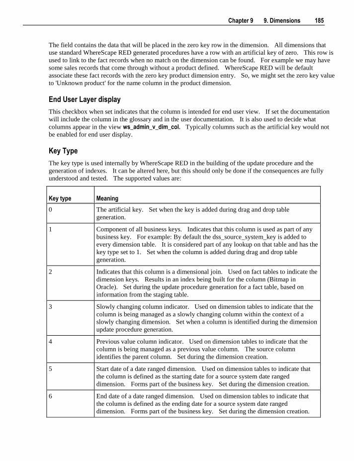
Chapter 9 9. Dimensions 185
The field contains the data that will be placed in the zero key row in the dimension. All dimensions that
use standard WhereScape RED generated procedures have a row with an artificial key of zero. This row is
used to link to the fact records when no match on the dimension can be found. For example we may have
some sales records that come through without a product defined. WhereScape RED will be default
associate these fact records with the zero key product dimension entry. So, we might set the zero key value
to 'Unknown product' for the name column in the product dimension.
End User Layer display
This checkbox when set indicates that the column is intended for end user view. If set the documentation
will include the column in the glossary and in the user documentation. It is also used to decide what
columns appear in the view ws_admin_v_dim_col. Typically columns such as the artificial key would not
be enabled for end user display.
Key Type
The key type is used internally by WhereScape RED in the building of the update procedure and the
generation of indexes. It can be altered here, but this should only be done if the consequences are fully
understood and tested. The supported values are:
Key type Meaning
0 The artificial key. Set when the key is added during drag and drop table
generation.
1 Component of all business keys. Indicates that this column is used as part of any
business key. For example: By default the dss_source_system_key is added to
every dimension table. It is considered part of any lookup on that table and has the
key type set to 1. Set when the column is added during drag and drop table
generation.
2 Indicates that this column is a dimensional join. Used on fact tables to indicate the
dimension keys. Results in an index being built for the column (Bitmap in
Oracle). Set during the update procedure generation for a fact table, based on
information from the staging table.
3 Slowly changing column indicator. Used on dimension tables to indicate that the
column is being managed as a slowly changing column within the context of a
slowly changing dimension. Set when a column is identified during the dimension
update procedure generation.
4 Previous value column indicator. Used on dimension tables to indicate that the
column is being managed as a previous value column. The source column
identifies the parent column. Set during the dimension creation.
5 Start date of a date ranged dimension. Used on dimension tables to indicate that
the column is defined as the starting date for a source system date ranged
dimension. Forms part of the business key. Set during the dimension creation.
6 End date of a date ranged dimension. Used on dimension tables to indicate that
the column is defined as the ending date for a source system date ranged
dimension. Forms part of the business key. Set during the dimension creation.
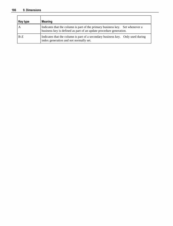
186 9. Dimensions
Key type Meaning
A Indicates that the column is part of the primary business key. Set whenever a
business key is defined as part of an update procedure generation.
B-Z Indicates that the column is part of a secondary business key. Only used during
index generation and not normally set.
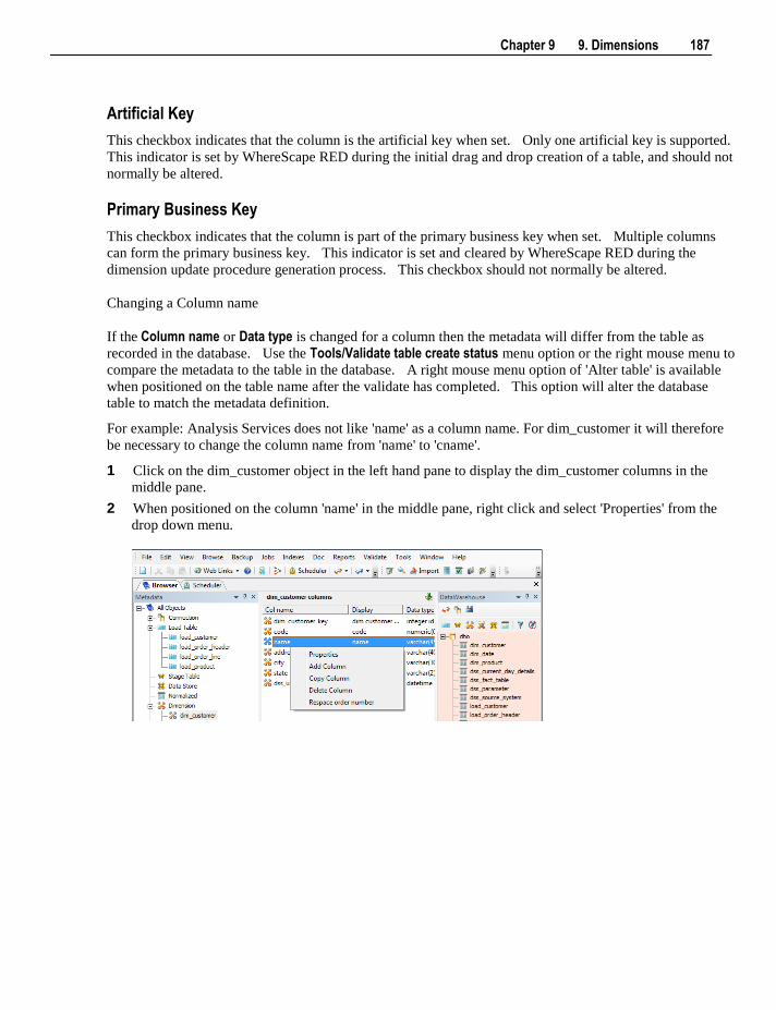
Chapter 9 9. Dimensions 187
Artificial Key
This checkbox indicates that the column is the artificial key when set. Only one artificial key is supported.
This indicator is set by WhereScape RED during the initial drag and drop creation of a table, and should not
normally be altered.
Primary Business Key
This checkbox indicates that the column is part of the primary business key when set. Multiple columns
can form the primary business key. This indicator is set and cleared by WhereScape RED during the
dimension update procedure generation process. This checkbox should not normally be altered.
Changing a Column name
If the Column name or Data type is changed for a column then the metadata will differ from the table as
recorded in the database. Use the Tools/Validate table create status menu option or the right mouse menu to
compare the metadata to the table in the database. A right mouse menu option of 'Alter table' is available
when positioned on the table name after the validate has completed. This option will alter the database
table to match the metadata definition.
For example: Analysis Services does not like 'name' as a column name. For dim_customer it will therefore
be necessary to change the column name from 'name' to 'cname'.
1 Click on the dim_customer object in the left hand pane to display the dim_customer columns in the
middle pane.
2 When positioned on the column 'name' in the middle pane, right click and select 'Properties' from the
drop down menu.
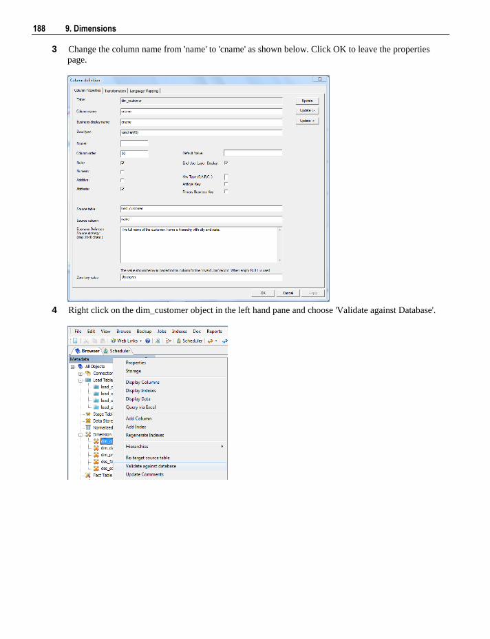
188 9. Dimensions
3 Change the column name from 'name' to 'cname' as shown below. Click OK to leave the properties
page.
4 Right click on the dim_customer object in the left hand pane and choose 'Validate against Database'.
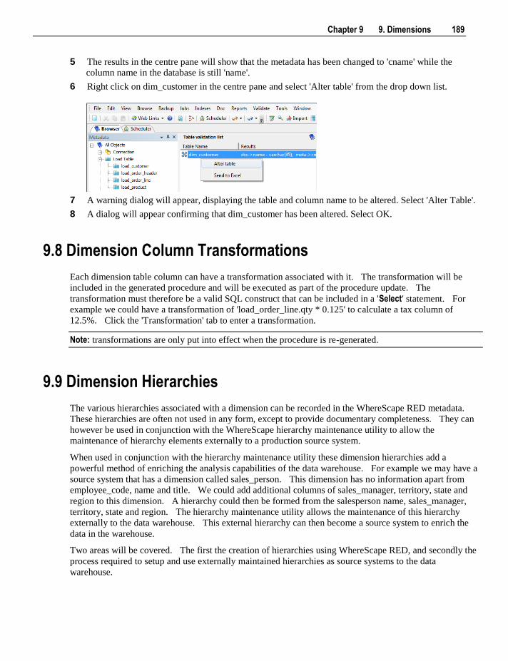
Chapter 9 9. Dimensions 189
5 The results in the centre pane will show that the metadata has been changed to 'cname' while the
column name in the database is still 'name'.
6 Right click on dim_customer in the centre pane and select 'Alter table' from the drop down list.
7 A warning dialog will appear, displaying the table and column name to be altered. Select 'Alter Table'.
8 A dialog will appear confirming that dim_customer has been altered. Select OK.
9.8 Dimension Column Transformations
Each dimension table column can have a transformation associated with it. The transformation will be
included in the generated procedure and will be executed as part of the procedure update. The
transformation must therefore be a valid SQL construct that can be included in a 'Select' statement. For
example we could have a transformation of 'load_order_line.qty * 0.125' to calculate a tax column of
12.5%. Click the 'Transformation' tab to enter a transformation.
Note: transformations are only put into effect when the procedure is re-generated.
9.9 Dimension Hierarchies
The various hierarchies associated with a dimension can be recorded in the WhereScape RED metadata.
These hierarchies are often not used in any form, except to provide documentary completeness. They can
however be used in conjunction with the WhereScape hierarchy maintenance utility to allow the
maintenance of hierarchy elements externally to a production source system.
When used in conjunction with the hierarchy maintenance utility these dimension hierarchies add a
powerful method of enriching the analysis capabilities of the data warehouse. For example we may have a
source system that has a dimension called sales_person. This dimension has no information apart from
employee_code, name and title. We could add additional columns of sales_manager, territory, state and
region to this dimension. A hierarchy could then be formed from the salesperson name, sales_manager,
territory, state and region. The hierarchy maintenance utility allows the maintenance of this hierarchy
externally to the data warehouse. This external hierarchy can then become a source system to enrich the
data in the warehouse.
Two areas will be covered. The first the creation of hierarchies using WhereScape RED, and secondly the
process required to setup and use externally maintained hierarchies as source systems to the data
warehouse.
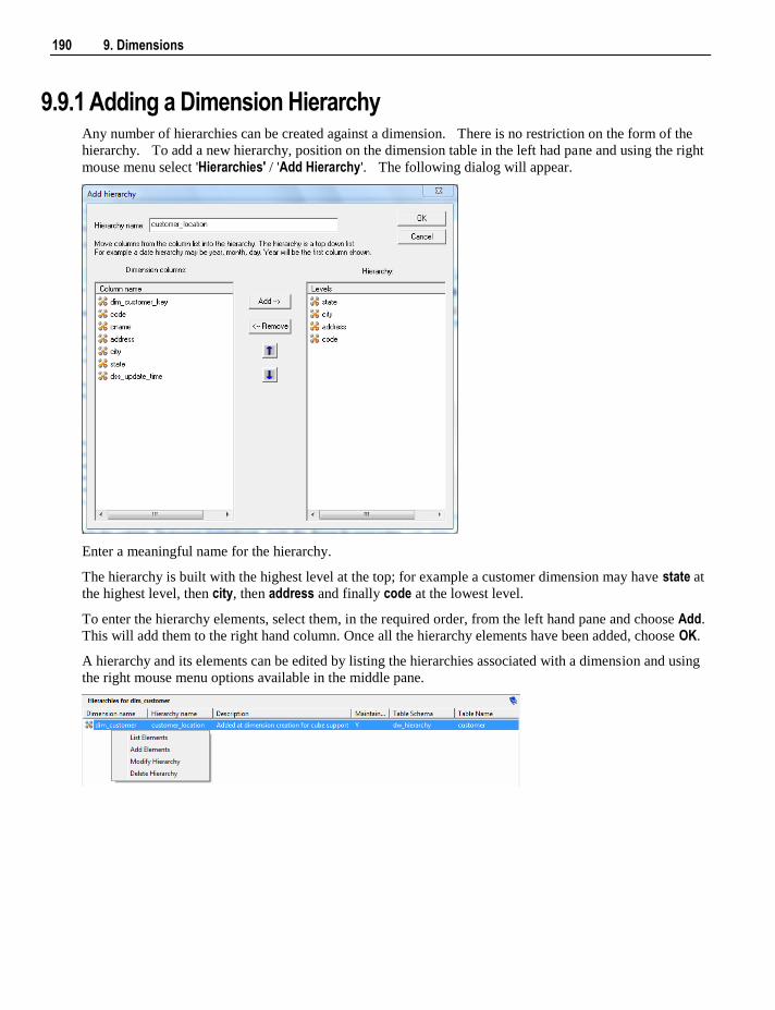
190 9. Dimensions
9.9.1 Adding a Dimension Hierarchy Any number of hierarchies can be created against a dimension. There is no restriction on the form of the
hierarchy. To add a new hierarchy, position on the dimension table in the left had pane and using the right
mouse menu select 'Hierarchies' / 'Add Hierarchy'. The following dialog will appear.
Enter a meaningful name for the hierarchy.
The hierarchy is built with the highest level at the top; for example a customer dimension may have state at
the highest level, then city, then address and finally code at the lowest level.
To enter the hierarchy elements, select them, in the required order, from the left hand pane and choose Add.
This will add them to the right hand column. Once all the hierarchy elements have been added, choose OK.
A hierarchy and its elements can be edited by listing the hierarchies associated with a dimension and using
the right mouse menu options available in the middle pane.
Chapter 9 9. Dimensions 191
9.9.2 Using a Maintained Hierarchy Once a hierarchy has been added to a dimension it can be maintained externally by the hierarchy
maintenance utility if the 'Maintained' attribute is set. The process for maintaining this hierarchy externally
and using it as a source system to the data warehouse is as follows.
1 Grant the user that is to undertake the maintenance select access to the following tables: ws_dim_tab,
ws_dim_col, ws_hie_header, ws_hie_link, ws_meta_tables.
2 Grant the user that is to undertake the maintenance select access to the dimension that has the
hierarchy.
3 Using the hierarchy maintenance utility (see online documentation) log on to the maintenance area and
create and populate/edit the maintenance table.
4 In WhereScape RED Create a connection to the hierarchy maintenance schema / database.
5 Browse the hierarchy connection.
6 Using drag and drop create a load table from the hierarchy maintenance table.
7 Edit the columns in the dimension that are to be sourced from the maintenance table and change their
source table and column to that of the load table and columns created in step 6.
8 Generate a new update procedure for the Dimension and either do a lookup of the maintenance table or
a join based on the business key.
9 Run the update procedure.
9.10 Snowflake
Snowflake schemas normalize dimensions to eliminate redundancy. That is, the dimension data has been
grouped into multiple tables instead of one large table. For example, a product dimension table in a star
schema might be normalized into a products table, a product_category table, and a product_manufacturer
table in a snowflake schema. While this saves space, it increases the number of dimension tables and
requires more foreign key joins. The result is more complex queries and reduced query performance.
9.10.1 Creating a Snowflake A snowflake dimensional structure is supported by WhereScape RED. A snowflake can be created for
normalized or partially normalized dimension tables. It is created by including the surrogate key of the
parent dimension in the child dimension. In the example below, the dim_state table represents the parent
dimension. The column dim_state_key is added to the child dimension dim_customer. Any fact tables
that include the dim_customer dimension will inherently have a link to the dim_state dimension.
The process for creating a snowflake is as follows:
1 Build both dimensions (see previous sections).
2 Expand dimensions in the left hand pane.
3 Click on the child dimension table in the left hand pane to display its columns in the centre pane.
4 Browse the data warehouse connection in the right hand pane.
5 Expand the parent dimension table in the right hand pane.
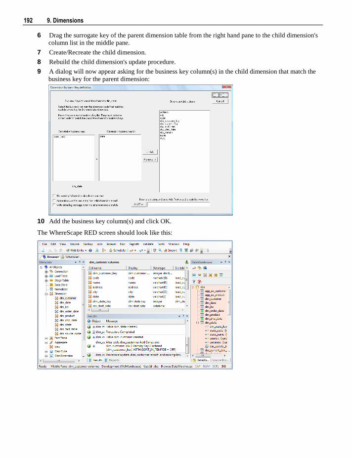
192 9. Dimensions
6 Drag the surrogate key of the parent dimension table from the right hand pane to the child dimension's
column list in the middle pane.
7 Create/Recreate the child dimension.
8 Rebuild the child dimension's update procedure.
9 A dialog will now appear asking for the business key column(s) in the child dimension that match the
business key for the parent dimension:
10 Add the business key column(s) and click OK.
The WhereScape RED screen should look like this:
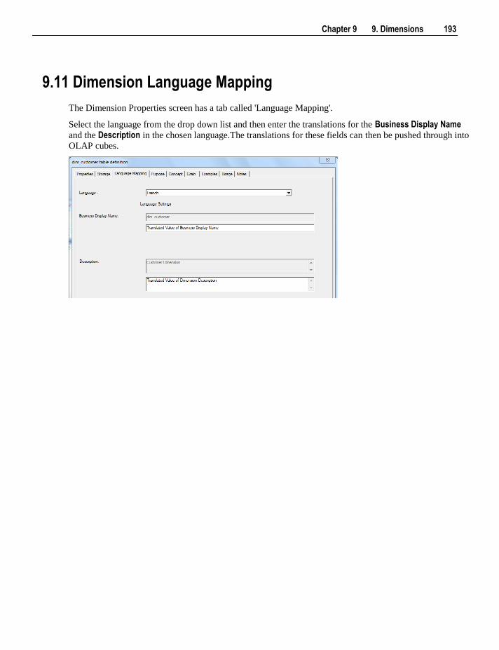
Chapter 9 9. Dimensions 193
9.11 Dimension Language Mapping
The Dimension Properties screen has a tab called 'Language Mapping'.
Select the language from the drop down list and then enter the translations for the Business Display Name
and the Description in the chosen language.The translations for these fields can then be pushed through into
OLAP cubes.

Chapter 10 10. Staging 195
Stage tables are used to transform the data to a star schema or third normal form model. A stage table can
be a fact or normalized table that only contains change data or a work table. In star schema data
warehouses, the stage table brings all the dimensional joins together in preparation for publishing into the
fact table.
A stage table is built from the Data Warehouse connection. Unless you are retrofitting an existing system,
stage tables are typically built from one or more load or stage tables. They can utilize the surrogate keys
from a number of dimension tables.
The normal steps for creating a stage table are defined below and are covered in this chapter. The steps
are:
Identify the source transactional data that will ultimately constitute the fact or normalized table. If the
data is sourced from multiple tables ascertain if a join between the source tables is possible, or if a
series of passes will be required to populate the stage table. If the latter option is chosen then bespoke
code is needed.
Using the 'drag and drop' functionality drag the table with the lowest granular data into a stage target.
See Building the Stage Table (see "10.1 Building the Stage Table" on page 196).
Add columns from other source tables. See Building the Stage Table (see "10.1 Building the Stage
Table" on page 196).
Add any relevant dimension table or normalized table keys. See Building the Stage Table (see "10.1
Building the Stage Table" on page 196).
Create the stage table in the database. See Building the Stage Table (see "10.1 Building the Stage
Table" on page 196).
Build the update procedure. See Generating the Staging Update Procedure (see "10.2 Generating
the Staging Update Procedure" on page 199).
Test the update procedure and analyze the results. See Tuning the Staging Update Process (see "10.3
Tuning the Staging Update Process" on page 210).
Modify the update procedure as required. See Tuning the Staging Update Process (see "10.3 Tuning
the Staging Update Process" on page 210).
In This Chapter
10.1 Building the Stage Table ..................................................... 196
10.2 Generating the Staging Update Procedure .......................... 199
10.3 Tuning the Staging Update Process ..................................... 210
10.4 Stage Table Column Properties ........................................... 211
10.5 Stage Table Column Transformations ................................. 216
C H A P T E R 1 0
10. Staging
196 10. Staging
10.1 Building the Stage Table
Building the stage table is potentially the most challenging part of the overall task of building a data
warehouse analysis area. Most of the effort required is in the design phase, in terms of knowing what data
needs to come into the fact table that will ultimately be built. This section assumes that the decision as to
what to include has been made.
Multiple data sources
A stage table typically contains the change data for a detail fact table. As such it normally maps to a
specific function within the business and in many cases relates back to one main OLTP table. In many
cases however it may be necessary to combine information from a number of tables. One of the decisions
required is whether or not it is practical or even possible to join the data from the different source tables.
In the tutorial the stage_sales_detail stage table is built by combining information from the order_header
table and the order_line table. These two tables are connected via the order_number field which is
common to both tables. The tutorial shows the building of a stage table and the joining of these two tables.
We could however also include two additional source tables being invoice_header and invoice_line which
contain specific information relating to what was on the invoice. We may want our fact table to contain
information from these tables as well. Although these two tables may contain the order_number and hence
potentially allow a join with the order tables we may choose not to perform such a join for performance
reasons. In such a situation we have three obvious choices in terms of how we ultimately update our fact
table. These are:
1 Join all four tables in one large join in our staging table.
2 Update the staging table in two passes. One pass updating the order information and one pass
updating the invoice information.
3 Generate two stage tables, one for order and one for invoice. Use these two staging tables to update
the one sales_detail fact table.
Although all three options are viable and a normal situation in the WhereScape RED environment, options
(2) and (3) will require specific coding and modifications to the generated procedures from the outset.
Given the example provided option (2) would be the normal approach, although in some cases option (3)
would be valid.
Drag and Drop
The best approach in creating a stage table is to choose the source table that contains the most fields that we
will be using and drag this table into the stage target. Then drag specific columns from the other source
tables until we have all the source data that is required.
The process for defining the metadata is as follows:
1 Double click on the 'Stage Table' object group in the left hand pane. This will result in all existing
stage tables being displayed in the middle pane. This also sets the middle pane as a stage drop target.
2 Browse the Data warehouse connection to display our load tables in the right hand pane. This is
achieved via the Browse/Source Tables menu option and then choosing the Data warehouse connection.
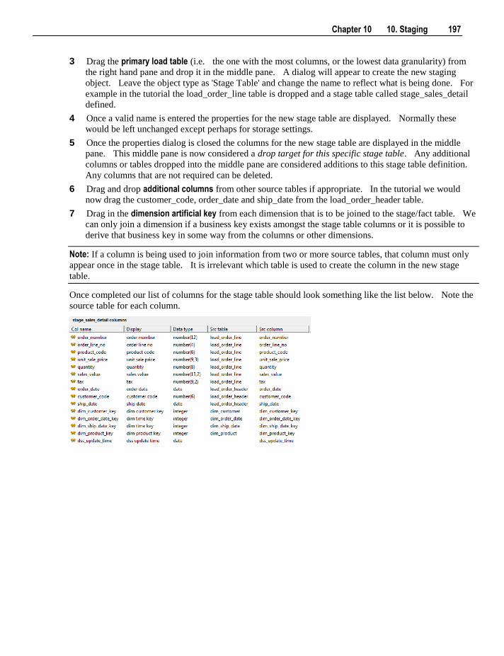
Chapter 10 10. Staging 197
3 Drag the primary load table (i.e. the one with the most columns, or the lowest data granularity) from
the right hand pane and drop it in the middle pane. A dialog will appear to create the new staging
object. Leave the object type as 'Stage Table' and change the name to reflect what is being done. For
example in the tutorial the load_order_line table is dropped and a stage table called stage_sales_detail
defined.
4 Once a valid name is entered the properties for the new stage table are displayed. Normally these
would be left unchanged except perhaps for storage settings.
5 Once the properties dialog is closed the columns for the new stage table are displayed in the middle
pane. This middle pane is now considered a drop target for this specific stage table. Any additional
columns or tables dropped into the middle pane are considered additions to this stage table definition.
Any columns that are not required can be deleted.
6 Drag and drop additional columns from other source tables if appropriate. In the tutorial we would
now drag the customer_code, order_date and ship_date from the load_order_header table.
7 Drag in the dimension artificial key from each dimension that is to be joined to the stage/fact table. We
can only join a dimension if a business key exists amongst the stage table columns or it is possible to
derive that business key in some way from the columns or other dimensions.
Note: If a column is being used to join information from two or more source tables, that column must only
appear once in the stage table. It is irrelevant which table is used to create the column in the new stage
table.
Once completed our list of columns for the stage table should look something like the list below. Note the
source table for each column.
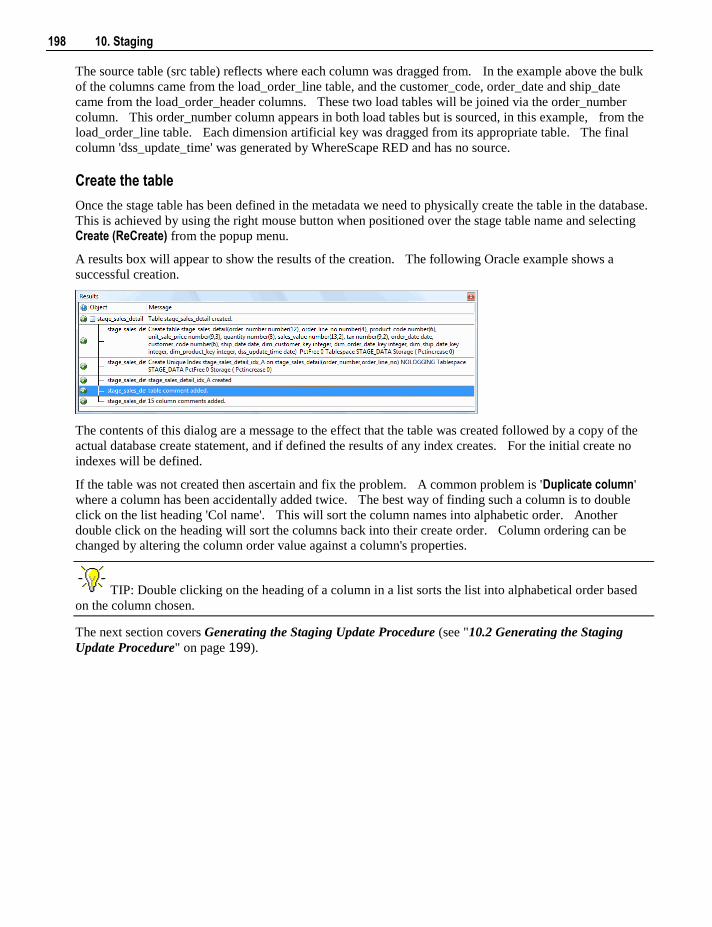
198 10. Staging
The source table (src table) reflects where each column was dragged from. In the example above the bulk
of the columns came from the load_order_line table, and the customer_code, order_date and ship_date
came from the load_order_header columns. These two load tables will be joined via the order_number
column. This order_number column appears in both load tables but is sourced, in this example, from the
load_order_line table. Each dimension artificial key was dragged from its appropriate table. The final
column 'dss_update_time' was generated by WhereScape RED and has no source.
Create the table
Once the stage table has been defined in the metadata we need to physically create the table in the database.
This is achieved by using the right mouse button when positioned over the stage table name and selecting
Create (ReCreate) from the popup menu.
A results box will appear to show the results of the creation. The following Oracle example shows a
successful creation.
The contents of this dialog are a message to the effect that the table was created followed by a copy of the
actual database create statement, and if defined the results of any index creates. For the initial create no
indexes will be defined.
If the table was not created then ascertain and fix the problem. A common problem is 'Duplicate column'
where a column has been accidentally added twice. The best way of finding such a column is to double
click on the list heading 'Col name'. This will sort the column names into alphabetic order. Another
double click on the heading will sort the columns back into their create order. Column ordering can be
changed by altering the column order value against a column's properties.
TIP: Double clicking on the heading of a column in a list sorts the list into alphabetical order based
on the column chosen.
The next section covers Generating the Staging Update Procedure (see "10.2 Generating the Staging
Update Procedure" on page 199).
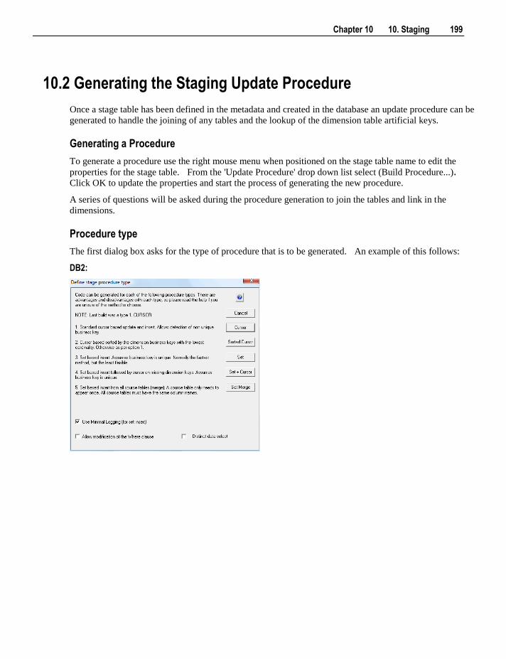
Chapter 10 10. Staging 199
10.2 Generating the Staging Update Procedure
Once a stage table has been defined in the metadata and created in the database an update procedure can be
generated to handle the joining of any tables and the lookup of the dimension table artificial keys.
Generating a Procedure
To generate a procedure use the right mouse menu when positioned on the stage table name to edit the
properties for the stage table. From the 'Update Procedure' drop down list select (Build Procedure...). Click OK to update the properties and start the process of generating the new procedure.
A series of questions will be asked during the procedure generation to join the tables and link in the
dimensions.
Procedure type
The first dialog box asks for the type of procedure that is to be generated. An example of this follows:
DB2:
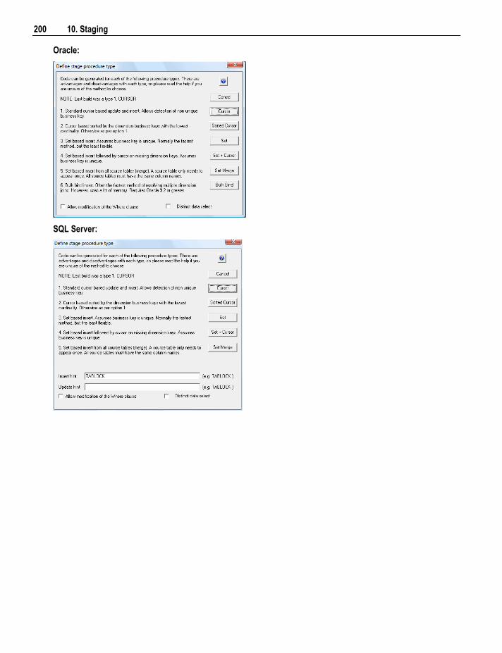
200 10. Staging
Oracle:
SQL Server:
Chapter 10 10. Staging 201
A number of different types of procedure generation are available. Each type is discussed below. There is
a check box at the bottom of the dialog box. This check box will only be present if advanced procedure
building features are enabled. This check box allows the editing of the 'Where' clause when no table joining
is being performed, and hence the where clause would not be exposed.
Cursor based procedure
This option creates a procedure that loops through each source transaction performing specific tasks on each
transaction before writing the transaction to the stage table. The tasks performed include the lookup of
each dimension key, and any bespoke value assignments or adjustments.
Sorted cursor procedure
This is a variant on the regular cursor procedure. In this case dimension key lookups only occur when
there is a change in the business key for a given dimension. This can improve the performance of the
procedure particularly when one or more of the dimensions has a low cardinality. Where slowly changing
dimensions are used this advantage is lessened as the relative date of the dimension records also comes into
play.
Set based procedure
A set based procedure performs one SQL statement to join all the dimensions and source tables together and
then insert this data into the stage table. This is normally the fastest method of building the stage table. It
is also the least flexible method and is easily prone to incorrect syntax. Care and experience must be used
with this option to ensure that all source transactions are processed and that they are processed correctly.
This option is only recommended for the experienced practitioner where performance is the overriding
requirement. Particular care must be taken with regards to NULL values in the business keys that are used
to make the table joins. The generated code deliberately does not handle such null values.
Set + Cursor Procedure
This option is normally used where a number of dimension keys will fail to join and we wish to
automatically add new dimension records. The first phase of the generated code will perform a set based
join and insert of the data. The dimensions that failed to join will be assigned the zero key value. The
second phase of the procedure will use a cursor to cycle through all the stage records that have a zero key
dimension join. By setting the appropriate flags in the dimension joins when building this procedure we
can request that any missing dimension records be automatically added.
Set Merge Procedure
This option is to allow the merging of two or more identical tables. The tables to be merged must have
exactly the same number of columns and column names. If necessary additional blank columns could be
added to one or other of the tables to make them identical. To use this procedure you must simply have the
tables to be merged mentioned at least once in the 'Source Table' field of a columns properties.
Bulk Bind Procedure
The bulk bind procedure is only available for Oracle. It uses memory arrays to join all the information
before writing it to the table. It can be the fastest method of performing a stage table update when a lot of
dimension joins are being used.
Note: The bulk bind procedure is only available for Oracle.
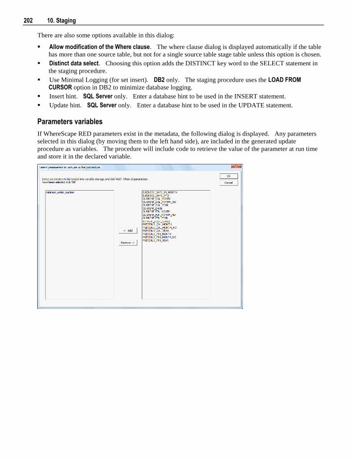
202 10. Staging
There are also some options available in this dialog:
Allow modification of the Where clause. The where clause dialog is displayed automatically if the table
has more than one source table, but not for a single source table stage table unless this option is chosen.
Distinct data select. Choosing this option adds the DISTINCT key word to the SELECT statement in
the staging procedure.
Use Minimal Logging (for set insert). DB2 only. The staging procedure uses the LOAD FROM CURSOR option in DB2 to minimize database logging.
Insert hint. SQL Server only. Enter a database hint to be used in the INSERT statement.
Update hint. SQL Server only. Enter a database hint to be used in the UPDATE statement.
Parameters variables
If WhereScape RED parameters exist in the metadata, the following dialog is displayed. Any parameters
selected in this dialog (by moving them to the left hand side), are included in the generated update
procedure as variables. The procedure will include code to retrieve the value of the parameter at run time
and store it in the declared variable.
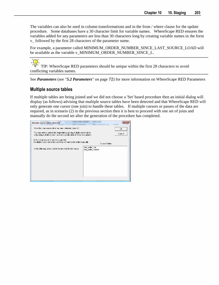
Chapter 10 10. Staging 203
The variables can also be used in column transformations and in the from / where clause for the update
procedure. Some databases have a 30 character limit for variable names. WhereScape RED ensures the
variables added for any parameters are less than 30 characters long by creating variable names in the form
v_ followed by the first 28 characters of the parameter name.
For example, a parameter called MINIMUM_ORDER_NUMBER_SINCE_LAST_SOURCE_LOAD will
be available as the variable v_MINIMUM_ORDER_NUMBER_SINCE_L.
TIP: WhereScape RED parameters should be unique within the first 28 characters to avoid
conflicting variables names.
See Parameters (see "5.2 Parameters" on page 72) for more information on WhereScape RED Parameters
Multiple source tables
If multiple tables are being joined and we did not choose a 'Set' based procedure then an initial dialog will
display (as follows) advising that multiple source tables have been detected and that WhereScape RED will
only generate one cursor (one join) to handle these tables. If multiple cursors or passes of the data are
required, as in scenario (2) in the previous section then it is best to proceed with one set of joins and
manually do the second set after the generation of the procedure has completed.
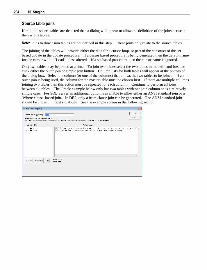
204 10. Staging
Source table joins
If multiple source tables are detected then a dialog will appear to allow the definition of the joins between
the various tables.
Note: Joins to dimension tables are not defined in this step. These joins only relate to the source tables.
The joining of the tables will provide either the data for a cursor loop, or part of the construct of the set
based update in the update procedure. If a cursor based procedure is being generated then the default name
for the cursor will be 'Load' unless altered. If a set based procedure then the cursor name is ignored.
Only two tables may be joined at a time. To join two tables select the two tables in the left hand box and
click either the outer join or simple join button. Column lists for both tables will appear at the bottom of
the dialog box. Select the column (or one of the columns) that allows the two tables to be joined. If an
outer join is being used, the column for the master table must be chosen first. If there are multiple columns
joining two tables then this action must be repeated for each column. Continue to perform all joins
between all tables. The Oracle example below only has two tables with one join column so is a relatively
simple case. For SQL Server an additional option is available to allow either an ANSI standard join or a
'Where clause' based join. In DB2, only a from clause join can be generated. The ANSI standard join
should be chosen in most situations. See the example screen in the following section.
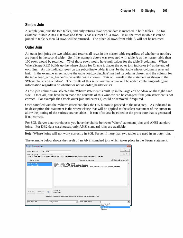
Chapter 10 10. Staging 205
Simple Join
A simple join joins the two tables, and only returns rows where data is matched in both tables. So for
example if table A has 100 rows and table B has a subset of 24 rows. If all the rows in table B can be
joined to table A then 24 rows will be returned. The other 76 rows from table A will not be returned.
Outer Join
An outer join joins the two tables, and returns all rows in the master table regardless of whether or not they
are found in the second table. So if the example above was executed with table A as the master table then
100 rows would be returned. 76 of those rows would have null values for the table B columns. When
WhereScape RED builds up the where clause for Oracle it places the outer join indicator (+) at the end of
each line. As this indicator goes on the subordinate table, it must be that table whose column is selected
last. In the example screen above the table 'load_order_line' has had its column chosen and the column for
the table 'load_order_header' is currently being chosen. This will result in the statement as shown in the
'Where clause edit window'. The results of this select are that a row will be added containing order_line
information regardless of whether or not an order_header exists.
As the join columns are selected the 'Where' statement is built up in the large edit window on the right hand
side. Once all joins have been made the contents of this window can be changed if the join statement is not
correct. For example the Oracle outer join indicator (+) could be removed if required.
Once satisfied with the 'Where' statement click the OK button to proceed to the next step. As indicated in
its description this statement is the where clause that will be applied to the select statement of the cursor to
allow the joining of the various source tables. It can of course be edited in the procedure that is generated
if not correct.
For SQL Server data warehouses you have the choice between 'Where' statement joins and ANSI standard
joins. For DB2 data warehouses, only ANSI standard joins are available.
Note: 'Where' joins will not work correctly in SQL Server if more than two tables are used in an outer join.
The example below shows the result of an ANSI standard join which takes place in the 'From' statement.
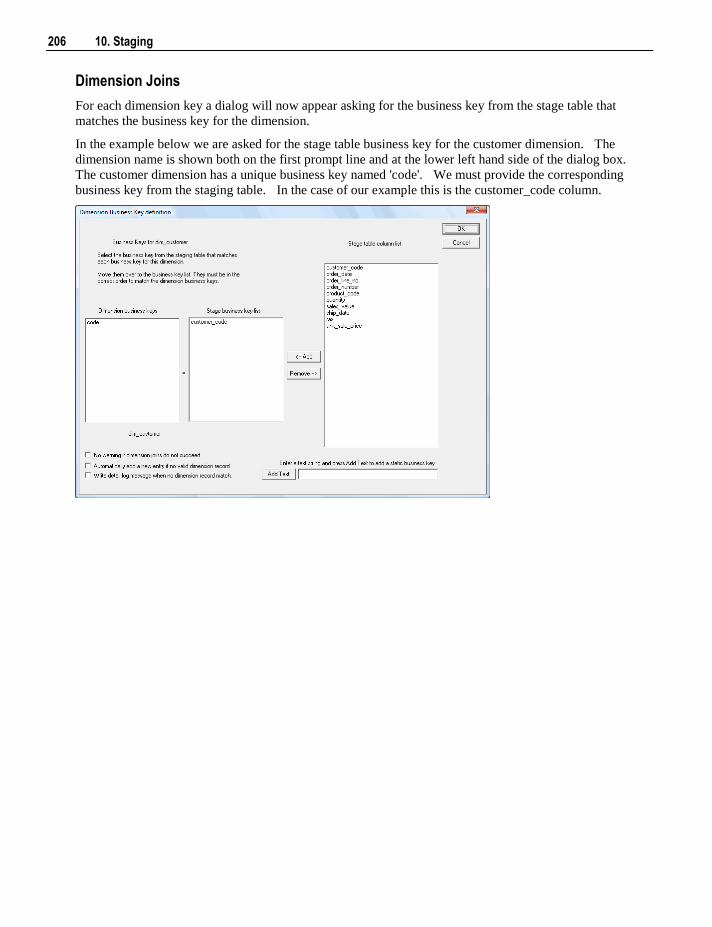
206 10. Staging
Dimension Joins
For each dimension key a dialog will now appear asking for the business key from the stage table that
matches the business key for the dimension.
In the example below we are asked for the stage table business key for the customer dimension. The
dimension name is shown both on the first prompt line and at the lower left hand side of the dialog box.
The customer dimension has a unique business key named 'code'. We must provide the corresponding
business key from the staging table. In the case of our example this is the customer_code column.
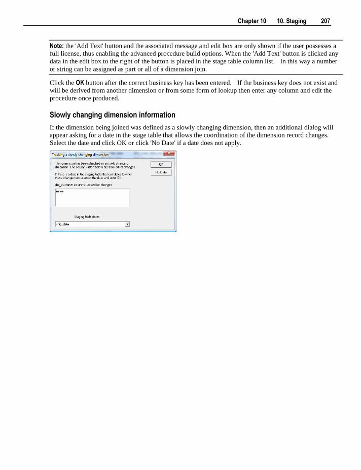
Chapter 10 10. Staging 207
Note: the 'Add Text' button and the associated message and edit box are only shown if the user possesses a
full license, thus enabling the advanced procedure build options. When the 'Add Text' button is clicked any
data in the edit box to the right of the button is placed in the stage table column list. In this way a number
or string can be assigned as part or all of a dimension join.
Click the OK button after the correct business key has been entered. If the business key does not exist and
will be derived from another dimension or from some form of lookup then enter any column and edit the
procedure once produced.
Slowly changing dimension information
If the dimension being joined was defined as a slowly changing dimension, then an additional dialog will
appear asking for a date in the stage table that allows the coordination of the dimension record changes.
Select the date and click OK or click 'No Date' if a date does not apply.
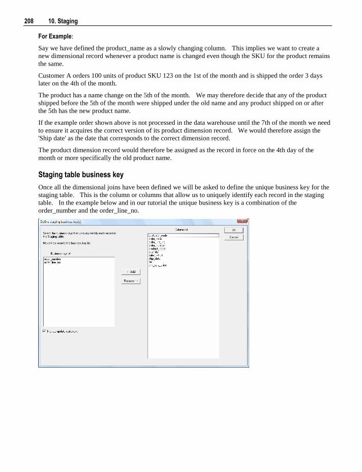
208 10. Staging
For Example:
Say we have defined the product_name as a slowly changing column. This implies we want to create a
new dimensional record whenever a product name is changed even though the SKU for the product remains
the same.
Customer A orders 100 units of product SKU 123 on the 1st of the month and is shipped the order 3 days
later on the 4th of the month.
The product has a name change on the 5th of the month. We may therefore decide that any of the product
shipped before the 5th of the month were shipped under the old name and any product shipped on or after
the 5th has the new product name.
If the example order shown above is not processed in the data warehouse until the 7th of the month we need
to ensure it acquires the correct version of its product dimension record. We would therefore assign the
'Ship date' as the date that corresponds to the correct dimension record.
The product dimension record would therefore be assigned as the record in force on the 4th day of the
month or more specifically the old product name.
Staging table business key
Once all the dimensional joins have been defined we will be asked to define the unique business key for the
staging table. This is the column or columns that allow us to uniquely identify each record in the staging
table. In the example below and in our tutorial the unique business key is a combination of the
order_number and the order_line_no.
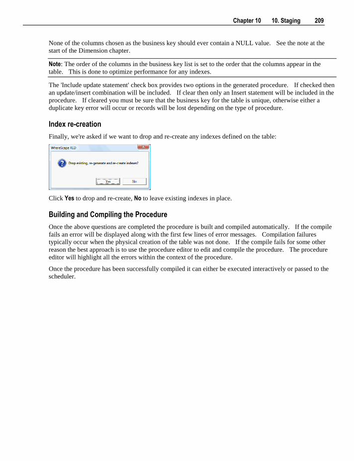
Chapter 10 10. Staging 209
None of the columns chosen as the business key should ever contain a NULL value. See the note at the
start of the Dimension chapter.
Note: The order of the columns in the business key list is set to the order that the columns appear in the
table. This is done to optimize performance for any indexes.
The 'Include update statement' check box provides two options in the generated procedure. If checked then
an update/insert combination will be included. If clear then only an Insert statement will be included in the
procedure. If cleared you must be sure that the business key for the table is unique, otherwise either a
duplicate key error will occur or records will be lost depending on the type of procedure.
Index re-creation
Finally, we're asked if we want to drop and re-create any indexes defined on the table:
Click Yes to drop and re-create, No to leave existing indexes in place.
Building and Compiling the Procedure
Once the above questions are completed the procedure is built and compiled automatically. If the compile
fails an error will be displayed along with the first few lines of error messages. Compilation failures
typically occur when the physical creation of the table was not done. If the compile fails for some other
reason the best approach is to use the procedure editor to edit and compile the procedure. The procedure
editor will highlight all the errors within the context of the procedure.
Once the procedure has been successfully compiled it can either be executed interactively or passed to the
scheduler.
210 10. Staging
10.3 Tuning the Staging Update Process
This section is for Cursor based procedures only. It is not relevant for Set based or other types.
When generating the cursor based procedures to update the staging table WhereScape RED includes
Update/Insert logic. This logic first attempts to update an existing staging record and then inserts a new
record if the record does not exist. This build option should be altered once an understanding of the data
you are dealing with is acquired.For the initial prototype and testing phases of a data warehouse analysis
area we need to find out if our business keys for the fact table are genuinely unique. The update/insert
logic in the staging procedure will only perform an 'Update' if our business key is not unique. In such a
situation we need to decide if this is a failure in the business key, or some form of additive record situation
we need to handle and code accordingly.
Removing the Update Component
Once we have resolved any data issues we would normally remove the update component to speed up the
processing of the stage data. There are two ways of doing this. Firstly we can clear the 'Include update
statement' check box when defining the table business key. This will result in a procedure with only an
insert statement. The other option is to do it manually as follows:
There are normally three steps to removing the update component. These being:
1 The update makes use of an index that can also be deleted in most situations.
2 The actual 'Update' statement can be removed from the code such that the insert is always executed.
3 The procedure also includes an analyze of the table after 1000 rows have been inserted. This code is
present to ensure that the index is used in the update. We can now remove this code. It would
normally look like the following (Oracle version):
--=======================================
-- If 1000 or more rows inserted then perform an analyze
--=======================================
IF v_insert_count >= 1000 And v_analyze_flag = 0 THEN
v_analyze_flag := 1;
v_Sql := 'analyze table stage estimate statistics sample 5 percent for all indexed columns';
execute immediate v_Sql;
END IF;
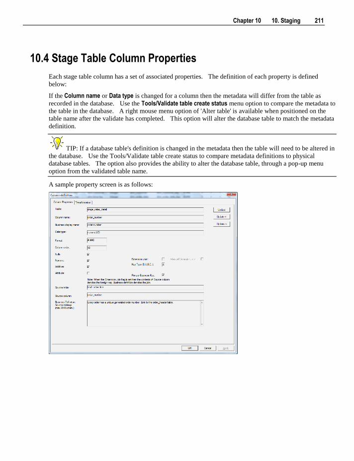
Chapter 10 10. Staging 211
10.4 Stage Table Column Properties
Each stage table column has a set of associated properties. The definition of each property is defined
below:
If the Column name or Data type is changed for a column then the metadata will differ from the table as
recorded in the database. Use the Tools/Validate table create status menu option to compare the metadata to
the table in the database. A right mouse menu option of 'Alter table' is available when positioned on the
table name after the validate has completed. This option will alter the database table to match the metadata
definition.
TIP: If a database table's definition is changed in the metadata then the table will need to be altered in
the database. Use the Tools/Validate table create status to compare metadata definitions to physical
database tables. The option also provides the ability to alter the database table, through a pop-up menu
option from the validated table name.
A sample property screen is as follows:
212 10. Staging
The two special update keys allow you to update the column and step either forward or backward to the
next column's properties. ALT-Left Arrow and ALT-Right Arrow can also be used instead of the two special
update keys.
Table
The table to which the column belongs. Read only.
Column name
The database name of the column. This name must conform to database column naming standards.
Typically such standards exclude the use of spaces etc. A good practice is to only use alphanumerics and
the underscore character. Changing this field alters the table's definition.
Business display name
This defines how the business refers to this column. Although it would not be normal practise to provide
end user access to stage tables, the contents of this field are passed through to the fact table during the drag
and drop operation, so this field can be commented for later use in the fact table if desired. This field does
not affect the physical table definition.
Data type
This is the database specific data type. It must be a valid data type for the data warehouse database
platform. Typical Oracle data types are number, char(), varchar2() and date. SQL Server databases often
have integer, numeric, varchar(), and datetime data types. See the database documentation for a
description of the data types available. Changing this field alters the table's definition.
Format
This field is to allow the definition of a format mask for end user tools. It does not affect the physical table
definition. This field would not normally be populated.
Column order
This numeric field provides the ordering of the columns in the database table create statement. The lowest
numbered column will appear first in the table. Although this affects the physical table definition no action
will be taken unless the table is re-created in the database. The columns can be re-numbered based on the
existing order by choosing the 'Respace order number' pop-up menu option when positioned over any
column in the table. This action will number the columns in increments of 10 starting at 10. In addition to
a simple change of the order field, the column order can be changed by first displaying the columns in the
middle pane and then using drag and drop to move the columns around. This drag and drop process will
automatically renumber the columns as required.
Nulls
This checkbox when set allows nulls to exist in this column. If cleared then nulls are not permitted in the
column.
Numeric
This checkbox indicates that the column in question is numeric when set. This is normally only relevant
for fact tables and would not normally be used for stage tables.
Chapter 10 10. Staging 213
Additive
This checkbox indicates that the column in question is additive when set. This is normally only relevant
for fact tables and would not normally be used for stage tables.
Attribute
This checkbox indicates that the column in question is an attribute when set. This is normally only
relevant for fact tables and would not normally be used for stage tables.
Source table
Indicates the table from which the column was sourced. This source table is normally a load table, or a
dimension table within the data warehouse. If the column was sourced from multiple tables, then the
normal practice is to record one of the tables in this field and a comment listing all of the other tables in the
'Source strategy' field. This field is used when generating a procedure to update the stage table. It is also
used in the track back diagrams and in the documentation.
Source column
Indicates the column in the 'Source table' from which the column was sourced. Such a column is normally
a load table column, which in turn may have been a transformation or the combination of multiple columns.
This may also be a dimensional key where a dimension is being joined.
Business definition / Source strategy
Normally this field will contain the strategy for acquiring or populating a column. It is a useful place to
record specific problems with the source data.
In the case of dimension keys this field is used to show the join between the stage table and the dimension,
once it has been defined as part of the stage table update procedure generation.
Dimension Join
This checkbox is set by WhereScape RED during the building of the update procedure and should not
normally be altered. It indicates that the column in question provides a join to a dimension table. The
'Source table' and 'Source column' fields will provide the dimension table's side of the join.
Manual Dimension Join
This checkbox can be set to change the way the dimension table is looked up during the staging table update
procedure build. Enabling this option allows you to join to the dimension manually in the Cursor mapping
dialog (where the Where clause is built). The usual dialog for matching the dimension business key to a
column or columns in the staging table is not displayed if this option is enabled.
Key Type
The key type is used internally by WhereScape RED in the building of the update procedure and the
generation of indexes. It can be altered here, but this should only be done if the consequences are fully
understood and tested. The supported values are:
Key type Meaning
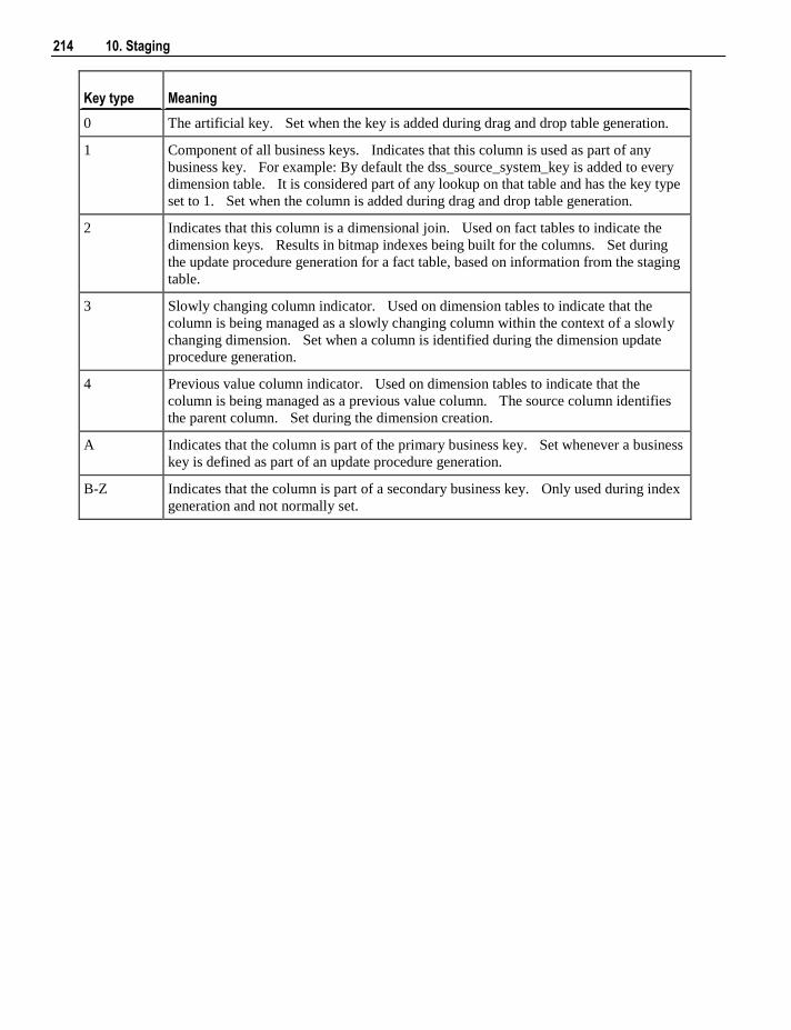
214 10. Staging
Key type Meaning
0 The artificial key. Set when the key is added during drag and drop table generation.
1 Component of all business keys. Indicates that this column is used as part of any
business key. For example: By default the dss_source_system_key is added to every
dimension table. It is considered part of any lookup on that table and has the key type
set to 1. Set when the column is added during drag and drop table generation.
2 Indicates that this column is a dimensional join. Used on fact tables to indicate the
dimension keys. Results in bitmap indexes being built for the columns. Set during
the update procedure generation for a fact table, based on information from the staging
table.
3 Slowly changing column indicator. Used on dimension tables to indicate that the
column is being managed as a slowly changing column within the context of a slowly
changing dimension. Set when a column is identified during the dimension update
procedure generation.
4 Previous value column indicator. Used on dimension tables to indicate that the
column is being managed as a previous value column. The source column identifies
the parent column. Set during the dimension creation.
A Indicates that the column is part of the primary business key. Set whenever a business
key is defined as part of an update procedure generation.
B-Z Indicates that the column is part of a secondary business key. Only used during index
generation and not normally set.
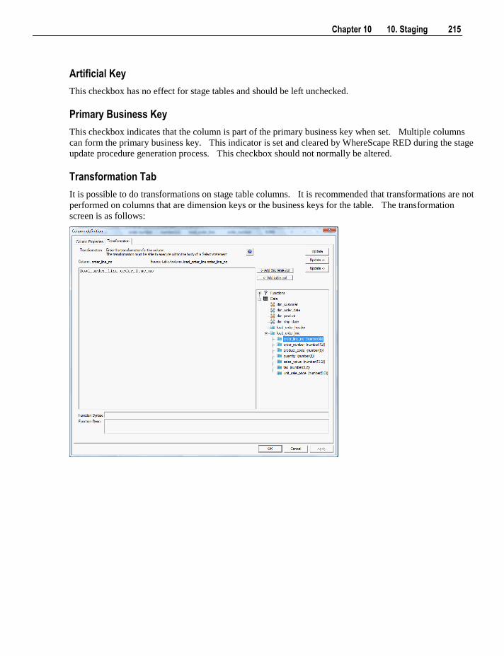
Chapter 10 10. Staging 215
Artificial Key
This checkbox has no effect for stage tables and should be left unchecked.
Primary Business Key
This checkbox indicates that the column is part of the primary business key when set. Multiple columns
can form the primary business key. This indicator is set and cleared by WhereScape RED during the stage
update procedure generation process. This checkbox should not normally be altered.
Transformation Tab
It is possible to do transformations on stage table columns. It is recommended that transformations are not
performed on columns that are dimension keys or the business keys for the table. The transformation
screen is as follows:
216 10. Staging
10.5 Stage Table Column Transformations
Each stage table column can have a transformation associated with it. The transformation will be included
in the generated procedure and will be executed as part of the procedure update. The transformation must
therefore be a valid SQL construct that can be included in a 'Select' statement. For example we could have
a transformation of 'load_order_line.qty * 0.125' to calculate a tax column of 12.5%. Click the
'Transformation' tab to enter a transformation.
Note: transformations are only put into effect when the procedure is re-generated.
See Transformations (see "19. Transformations" on page 387) for more details.
Chapter 11 11. Data Store Objects 217
In This Chapter
11.1 Data Store Object Overview ............................................... 218
11.2 Building a Data Store Object .............................................. 220
11.3 Generating the Data Store Update Procedure...................... 224
11.4 Data Store Artificial Keys ................................................... 235
11.5 Data Store Column Properties ............................................. 237
11.6 Data Store Object Column Transformations ....................... 240
C H A P T E R 1 1
11. Data Store Objects
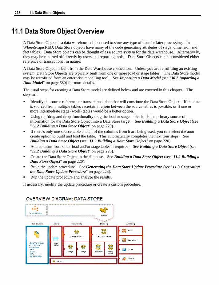
218 11. Data Store Objects
11.1 Data Store Object Overview
A Data Store Object is a data warehouse object used to store any type of data for later processing. In
WhereScape RED, Data Store objects have many of the code generating attributes of stage, dimension and
fact tables. Data Store objects can be thought of as a source system for the data warehouse. Alternatively,
they may be reported off directly by users and reporting tools. Data Store Objects can be considered either
reference or transactional in nature.
A Data Store Object is built from the Data Warehouse connection. Unless you are retrofitting an existing
system, Data Store Objects are typically built from one or more load or stage tables. The Data Store model
may be retrofitted from an enterprise modelling tool. See Importing a Data Model (see "30.2 Importing a
Data Model" on page 680) for more details.
The usual steps for creating a Data Store model are defined below and are covered in this chapter. The
steps are:
Identify the source reference or transactional data that will constitute the Data Store Object. If the data
is sourced from multiple tables ascertain if a join between the source tables is possible, or if one or
more intermediate stage (work) tables would be a better option.
Using the 'drag and drop' functionality drag the load or stage table that is the primary source of
information for the Data Store Object into a Data Store target. See Building a Data Store Object (see
"11.2 Building a Data Store Object" on page 220).
If there's only one source table and all of the columns from it are being used, you can select the auto
create option to build and load the table. This automatically completes the next four steps. See
Building a Data Store Object (see "11.2 Building a Data Store Object" on page 220).
Add columns from other load and/or stage tables if required. See Building a Data Store Object (see
"11.2 Building a Data Store Object" on page 220).
Create the Data Store Object in the database. See Building a Data Store Object (see "11.2 Building a
Data Store Object" on page 220).
Build the update procedure. See Generating the Data Store Update Procedure (see "11.3 Generating
the Data Store Update Procedure" on page 224).
Run the update procedure and analyze the results.
If necessary, modify the update procedure or create a custom procedure.
Chapter 11 11. Data Store Objects 219
Data Store Object Keys
Data Store Objects have Business Keys, they do not usually have Artificial Keys.
Business Key
The business key is the column or columns that uniquely identify a record within a Data Store Object.
Where the Data Store Object maps back to a single or a main table in the source system, it is usually
possible to ascertain the business key by looking at the unique keys for that source table. The business key
is sometimes referred to as the 'natural' key. Examples of business keys are:
The product SKU in a product table
The customer code in a customer table
The IATA airport code in an airport table.
It is assumed that business keys will never be NULL. If a null value is possible in a business key then the
generated code will need to be modified to handle the null value by assigning some default value. In the
following examples, the business key column is modified by using a database function and default value:
DB2: COALESCE(business_key,'N/A')
SQL Server: ISNULL(business_key,'N/A')
Oracle: NVL(business_key,'N/A')
Note: Business keys are assumed to never be Null. If they can be null it is best to transform them to some
value prior to the Data Store or stage table update. If this is not done, an un-modified update procedure
will probably fail with a duplicate key error on the business key index.
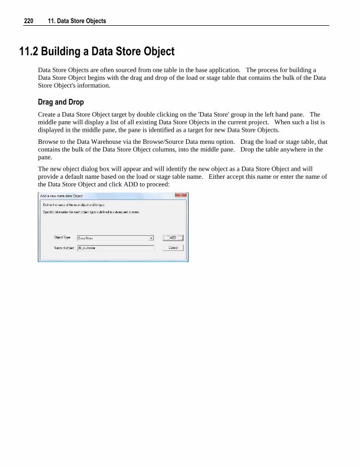
220 11. Data Store Objects
11.2 Building a Data Store Object
Data Store Objects are often sourced from one table in the base application. The process for building a
Data Store Object begins with the drag and drop of the load or stage table that contains the bulk of the Data
Store Object's information.
Drag and Drop
Create a Data Store Object target by double clicking on the 'Data Store' group in the left hand pane. The
middle pane will display a list of all existing Data Store Objects in the current project. When such a list is
displayed in the middle pane, the pane is identified as a target for new Data Store Objects.
Browse to the Data Warehouse via the Browse/Source Data menu option. Drag the load or stage table, that
contains the bulk of the Data Store Object columns, into the middle pane. Drop the table anywhere in the
pane.
The new object dialog box will appear and will identify the new object as a Data Store Object and will
provide a default name based on the load or stage table name. Either accept this name or enter the name of
the Data Store Object and click ADD to proceed:
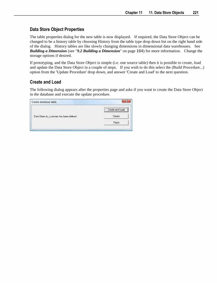
Chapter 11 11. Data Store Objects 221
Data Store Object Properties
The table properties dialog for the new table is now displayed. If required, the Data Store Object can be
changed to be a history table by choosing History from the table type drop down list on the right hand side
of the dialog. History tables are like slowly changing dimensions in dimensional data warehouses. See
Building a Dimension (see "9.2 Building a Dimension" on page 164) for more information. Change the
storage options if desired.
If prototyping, and the Data Store Object is simple (i.e. one source table) then it is possible to create, load
and update the Data Store Object in a couple of steps. If you wish to do this select the (Build Procedure...)
option from the 'Update Procedure' drop down, and answer 'Create and Load' to the next question.
Create and Load
The following dialog appears after the properties page and asks if you want to create the Data Store Object
in the database and execute the update procedure.
222 11. Data Store Objects
If you are satisfied with the columns that will be used and do not wish to add additional columns you can
select the Create and Load button. In such an event it would be normal practice to select the (Build
Procedure...) option from the 'Update Procedure' drop down box in the previous properties page. If no
procedure has been selected then select the Create button as no update will occur in any event.
If Create or Create and Load is selected and a new procedure creation was chosen proceed directly to the
Generating the Update Procedure (see "12.3 Generating the Normalized Update Procedure" on page 248)
section.
If you have additional columns to add or columns to delete then select Finish and proceed as follows.
Deleting and Changing columns
The columns defined for the Data Store Object will be displayed in the middle pane. It is possible to delete
any unwanted columns by highlighting a column name or a group of names and pushing the 'Delete' key.
The name of a column can also be changed by selecting the column and using the right mouse menu to edit
its properties. Any new name must conform to the database naming standards. Good practice is to use
alphanumerics and the underscore character. See the section on column properties for a fuller description
on what the various fields mean.
TIP: When prototyping, and in the initial stages of an analysis area build it is best not to remove
columns, nor to change their names to any great extent. This type of activity is best left until after end
users have used the data and provided feedback.
Adding additional columns
With the columns of the Data Store Object displayed in the middle pane, this pane is considered a drop
target for additional columns.
It is a simple matter to select columns from other load and/or stage tables and drag these columns into the
middle pane. The source table column in the middle pane shows where each column was dragged from.
The column description could be acquired from three different tables. The best practise is to rename at
least two of the columns, perhaps also adding context to the column name. For example, description could
become group_description, and so forth.
There are a number of WhereScape RED ancillary columns that do not have a source table. These columns
have been added by WhereScape RED, and are added depending on earlier choices. A description of these
columns follows.
Column name description
dss_start_date Used for history tables. This column provides a date time stamp when
the Data Store Object record came into existence. It is used to ascertain
which Data Store Object record should be used when multiple are
available.
dss_end_date Used for history tables. This column provides a date time stamp when
the Data Store Object record ceased to be the current record. It is used
to ascertain which Data Store Object record should be used when
multiple are available.
dss_current_flag Used for Data Store history tables. This flag identifies the current
record where multiple versions exist.
Chapter 11 11. Data Store Objects 223
Column name description
dss_source_system_key Added to support history tables that cannot be fully conformed, and the
inclusion of subsequent source systems. See the ancillary settings
section for more details.
dss_version Used for Data Store history tables. This column contains the version
number of a Data Store history tables record. Numbered from 1
upwards with the highest number being the latest or current version. It
forms part of the unique constraint for the business key of a Data Store
history tables.
dss_update_time Indicates when the record was last updated in the data warehouse.
dss_create_time Indicates when the record was first created in the data warehouse
Create the table
Once the Data Store Object has been defined in the metadata we need to physically create the table in the
database. This is achieved by using the right mouse button when positioned over the Data Store Object
name and selecting Create (ReCreate) from the popup menu.
A results dialog box will appear to show the results of the creation.
The contents of this dialog are a message to the effect that the Data Store Object was created. A copy of
the actual database create statement and if defined the results of any index create statements will be listed.
For the initial create no indexes will be defined.
If the table was not created then ascertain and fix the problem. A common problem is 'Duplicate column'
where a column has the same name in two of the source tables. The best way of finding such a column is
to double click on the list heading 'Col name'. This will sort the column names into alphabetic order.
Another double click on the heading will sort the columns back into their create order.
The next section covers Generating the Data Store Update Procedure (see "11.3 Generating the Data
Store Update Procedure" on page 224).
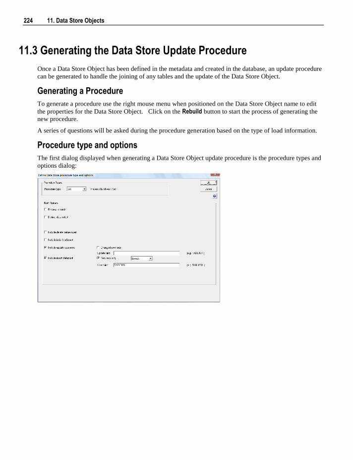
224 11. Data Store Objects
11.3 Generating the Data Store Update Procedure
Once a Data Store Object has been defined in the metadata and created in the database, an update procedure
can be generated to handle the joining of any tables and the update of the Data Store Object.
Generating a Procedure
To generate a procedure use the right mouse menu when positioned on the Data Store Object name to edit
the properties for the Data Store Object. Click on the Rebuild button to start the process of generating the
new procedure.
A series of questions will be asked during the procedure generation based on the type of load information.
Procedure type and options
The first dialog displayed when generating a Data Store Object update procedure is the procedure types and
options dialog:
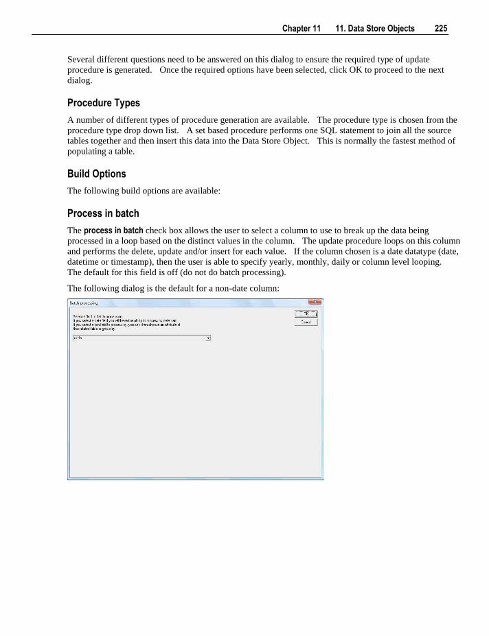
Chapter 11 11. Data Store Objects 225
Several different questions need to be answered on this dialog to ensure the required type of update
procedure is generated. Once the required options have been selected, click OK to proceed to the next
dialog.
Procedure Types
A number of different types of procedure generation are available. The procedure type is chosen from the
procedure type drop down list. A set based procedure performs one SQL statement to join all the source
tables together and then insert this data into the Data Store Object. This is normally the fastest method of
populating a table.
Build Options
The following build options are available:
Process in batch
The process in batch check box allows the user to select a column to use to break up the data being
processed in a loop based on the distinct values in the column. The update procedure loops on this column
and performs the delete, update and/or insert for each value. If the column chosen is a date datatype (date,
datetime or timestamp), then the user is able to specify yearly, monthly, daily or column level looping.
The default for this field is off (do not do batch processing).
The following dialog is the default for a non-date column:
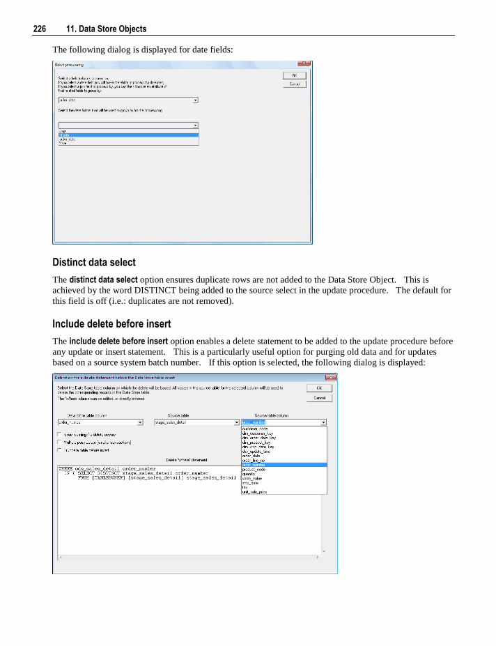
226 11. Data Store Objects
The following dialog is displayed for date fields:
Distinct data select
The distinct data select option ensures duplicate rows are not added to the Data Store Object. This is
achieved by the word DISTINCT being added to the source select in the update procedure. The default for
this field is off (i.e.: duplicates are not removed).
Include delete before insert
The include delete before insert option enables a delete statement to be added to the update procedure before
any update or insert statement. This is a particularly useful option for purging old data and for updates
based on a source system batch number. If this option is selected, the following dialog is displayed:
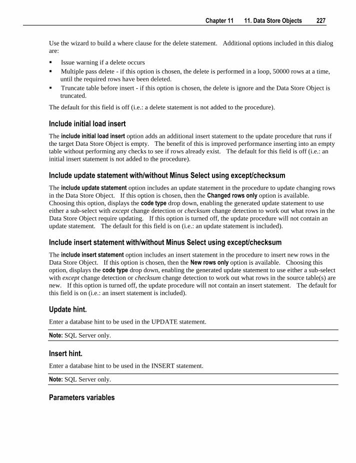
Chapter 11 11. Data Store Objects 227
Use the wizard to build a where clause for the delete statement. Additional options included in this dialog
are:
Issue warning if a delete occurs
Multiple pass delete - if this option is chosen, the delete is performed in a loop, 50000 rows at a time,
until the required rows have been deleted.
Truncate table before insert - if this option is chosen, the delete is ignore and the Data Store Object is
truncated.
The default for this field is off (i.e.: a delete statement is not added to the procedure).
Include initial load insert
The include initial load insert option adds an additional insert statement to the update procedure that runs if
the target Data Store Object is empty. The benefit of this is improved performance inserting into an empty
table without performing any checks to see if rows already exist. The default for this field is off (i.e.: an
initial insert statement is not added to the procedure).
Include update statement with/without Minus Select using except/checksum
The include update statement option includes an update statement in the procedure to update changing rows
in the Data Store Object. If this option is chosen, then the Changed rows only option is available.
Choosing this option, displays the code type drop down, enabling the generated update statement to use
either a sub-select with except change detection or checksum change detection to work out what rows in the
Data Store Object require updating. If this option is turned off, the update procedure will not contain an
update statement. The default for this field is on (i.e.: an update statement is included).
Include insert statement with/without Minus Select using except/checksum
The include insert statement option includes an insert statement in the procedure to insert new rows in the
Data Store Object. If this option is chosen, then the New rows only option is available. Choosing this
option, displays the code type drop down, enabling the generated update statement to use either a sub-select
with except change detection or checksum change detection to work out what rows in the source table(s) are
new. If this option is turned off, the update procedure will not contain an insert statement. The default for
this field is on (i.e.: an insert statement is included).
Update hint.
Enter a database hint to be used in the UPDATE statement.
Note: SQL Server only.
Insert hint.
Enter a database hint to be used in the INSERT statement.
Note: SQL Server only.
Parameters variables
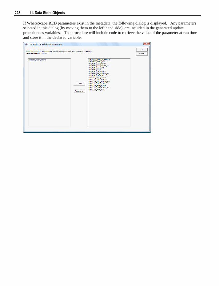
228 11. Data Store Objects
If WhereScape RED parameters exist in the metadata, the following dialog is displayed. Any parameters
selected in this dialog (by moving them to the left hand side), are included in the generated update
procedure as variables. The procedure will include code to retrieve the value of the parameter at run time
and store it in the declared variable.
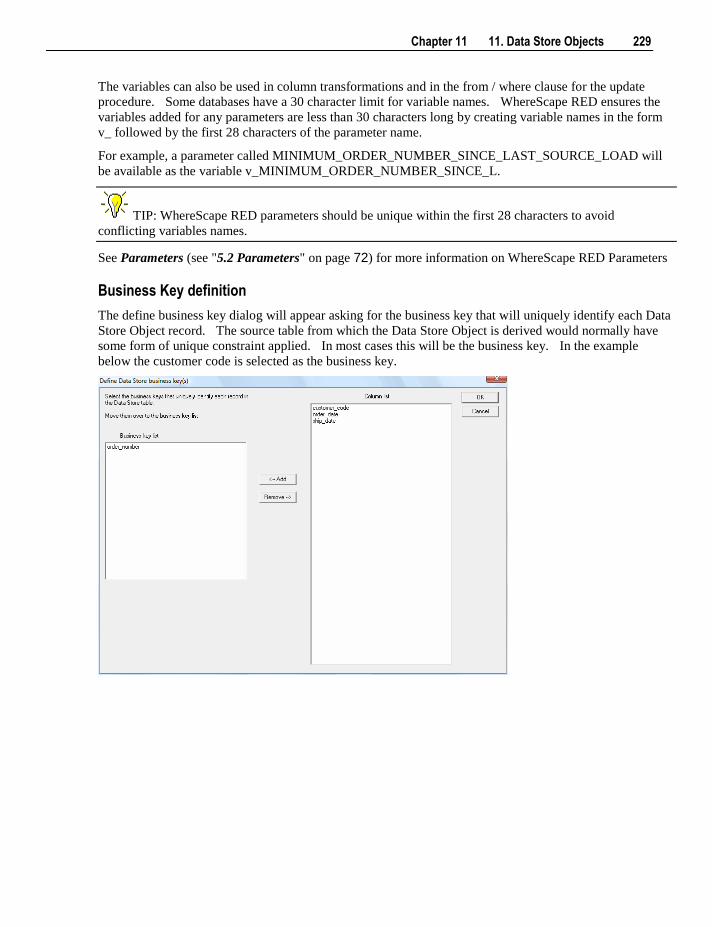
Chapter 11 11. Data Store Objects 229
The variables can also be used in column transformations and in the from / where clause for the update
procedure. Some databases have a 30 character limit for variable names. WhereScape RED ensures the
variables added for any parameters are less than 30 characters long by creating variable names in the form
v_ followed by the first 28 characters of the parameter name.
For example, a parameter called MINIMUM_ORDER_NUMBER_SINCE_LAST_SOURCE_LOAD will
be available as the variable v_MINIMUM_ORDER_NUMBER_SINCE_L.
TIP: WhereScape RED parameters should be unique within the first 28 characters to avoid
conflicting variables names.
See Parameters (see "5.2 Parameters" on page 72) for more information on WhereScape RED Parameters
Business Key definition
The define business key dialog will appear asking for the business key that will uniquely identify each Data
Store Object record. The source table from which the Data Store Object is derived would normally have
some form of unique constraint applied. In most cases this will be the business key. In the example
below the customer code is selected as the business key.
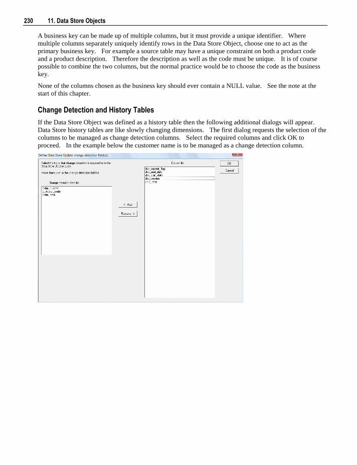
230 11. Data Store Objects
A business key can be made up of multiple columns, but it must provide a unique identifier. Where
multiple columns separately uniquely identify rows in the Data Store Object, choose one to act as the
primary business key. For example a source table may have a unique constraint on both a product code
and a product description. Therefore the description as well as the code must be unique. It is of course
possible to combine the two columns, but the normal practice would be to choose the code as the business
key.
None of the columns chosen as the business key should ever contain a NULL value. See the note at the
start of this chapter.
Change Detection and History Tables
If the Data Store Object was defined as a history table then the following additional dialogs will appear.
Data Store history tables are like slowly changing dimensions. The first dialog requests the selection of the
columns to be managed as change detection columns. Select the required columns and click OK to
proceed. In the example below the customer name is to be managed as a change detection column.
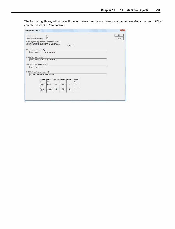
Chapter 11 11. Data Store Objects 231
The following dialog will appear if one or more columns are chosen as change detection columns. When
completed, click OK to continue.
232 11. Data Store Objects
Add null support
If the Add null support option is selected, then change detect column management will cater for null values
in any change detect columns. If this option is not selected, and null values are present, errors may occur
running the update procedure. The default for this value is off (i.e.: nulls are not catered for).
Update Current record only
The Update Current record only option will only apply changes to non-change detect columns on the current record. If this option is not selected, all past (non-current) rows will also be updated to reflect changes to
non-change detect columns. The default for this value is on (i.e.: only the current record is updated).
Start date for initial member
The Start date for initial member field contains the start date for the first version of a particular business key.
The value should be specified in an appropriate form, taking into account the default date format in the
databases. The date may need to be explicitly cast to the correct data type. The default value provided
will usually be cast to the correct datatype and can be treated as a template. The default value for this field
is 1 January 1900.
End date for current member
The End date for current member field contains the end date for the current version (the row with a current
flag of Y and the maximum version number) of a particular business key. The value should be specified in
an appropriate form, taking into account the default date format in the databases. The date may need to be
explicitly cast to the correct data type. The default value provided will usually be cast to the correct
datatype and can be treated as a template. The default value for this field is 31 December 2999.
Start date for new member entry
The Start date for new member entry field contains the start date for any subsequent rows added to the
history table (not the first row for a particular business key i.e.: not version 1). The value should be
specified in an appropriate form, taking into account the default date format in the databases. The date
may need to be explicitly cast to the correct data type. The default value provided will usually be cast to
the correct datatype and can be treated as a template. The default value for this field is the current date and
time.
End date for expiring member entry
The End date for expiring member entry field contains the end date for any rows updated to no longer be the
current row in the history table (i.e.: rows that are replaced by a new current row). The value should be
specified in an appropriate form, taking into account the default date format in the databases. The date
may need to be explicitly cast to the correct data type. The default value provided will usually be cast to
the correct datatype and can be treated as a template. The default value for this field is the current date and
time less an arbitrary small amount (for SQL Server this is 0.00000005 of a day, or about 4 thousandth of a
second.
Reset
Click on the Reset button to return all fields in this dialog to their default values.
Joining multiple source tables, where and group by clauses
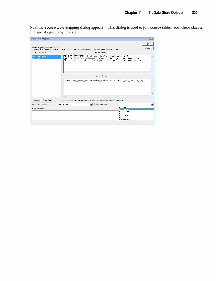
Chapter 11 11. Data Store Objects 233
Next the Source table mapping dialog appears. This dialog is used to join source tables, add where clauses
and specify group by clauses.
234 11. Data Store Objects
To join two tables, start by selecting the two tables in the left hand box and then clicking one of the join
buttons. The columns for the two tables then appear at the bottom of the dialog and one column is selected
from each drop down list to effect the join between the selected tables. In the example above the
load_prod_group and load_prod_subgroup tables are joined by the column prod_group. For multiple
column joins, repeat the join process.
Simple Join
A simple join only returns rows where data is matched in both tables. So for example if table A has 100
rows and table B has a subset of 24 rows. If all the rows in table B can be joined to table A then 24 rows
will be returned. The other 76 rows from table A will not be returned.
Outer Join
The outer join returns all rows in the master table regardless of whether or not they are found in the second
table. So if the example above was executed with table A as the master table then 100 rows would be
returned. 76 of those rows would have null values for the table B columns.
Note: When WhereScape RED builds up an outer join, it needs to know which table is the master table and
which is subordinate. Select the join column from the master table first. In the example screen above the
table 'load_prod_group' has had its column chosen and the column for the table 'load_prod_subgroup' is
currently being chosen. This will result in the 'load_prod_group' table being defined as the master, as per
the example statement above. The results of this example select are that a row will be added containing
product information regardless of whether or not a corresponding prod_subgroup entry exists.
As the join columns are selected the join statement is built up in the large edit window on the right hand
side. Once all joins have been made the contents of this window can be changed if the join statement is not
correct. For example the Oracle outer join indicator (+) could be removed if required.
Where Clause
A where clause can be manually added to the where clause field in this dialog.
Group By Clause
A group by clause (and any other clauses that come after the where clause) can be added to the group by
clause in this dialog.
Building and Compiling the Procedure
Once the above questions are completed the procedure is built and compiled automatically. If the compile
fails an error will be displayed along with the first few lines of error messages. Compile fails typically
occur when the physical creation of the table was not done. If the compile fails for some other reason the
best approach is to use the procedure editor to edit and compile the procedure. The procedure editor will
highlight all the errors within the context of the procedure.
Once the procedure has been successfully compiled it can either be executed interactively or passed to the
scheduler.
Indexes
By default a number of indexes will be created to support each Data Store Object. These indexes will be
added once the procedure has been built. An example of the type of indexes created is as follows:
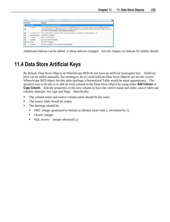
Chapter 11 11. Data Store Objects 235
Additional indexes can be added, or these indexes changed. See the chapter on indexes for further details.
11.4 Data Store Artificial Keys
By default, Data Store Objects in WhereScape RED do not have an artificial (surrogate) key. Artificial
keys can be added manually, but needing to do so could indicate Data Store Objects are not the correct
WhereScape RED object for this table (perhaps a Normalized Table would be more appropriate). The
quickest way to do this is to add an extra column to the Data Store Object by using either Add Column or
Copy Column. Edit the properties of the new column to have the correct name and order, source table and
column, datatype, key type and flags. Specifically:
The column name and source column name should be the same.
The source table should be empty.
The datatype should be:
DB2: integer generated by default as identity (start with 1, increment by 1)
Oracle: integer
SQL Server: integer identity(0,1)
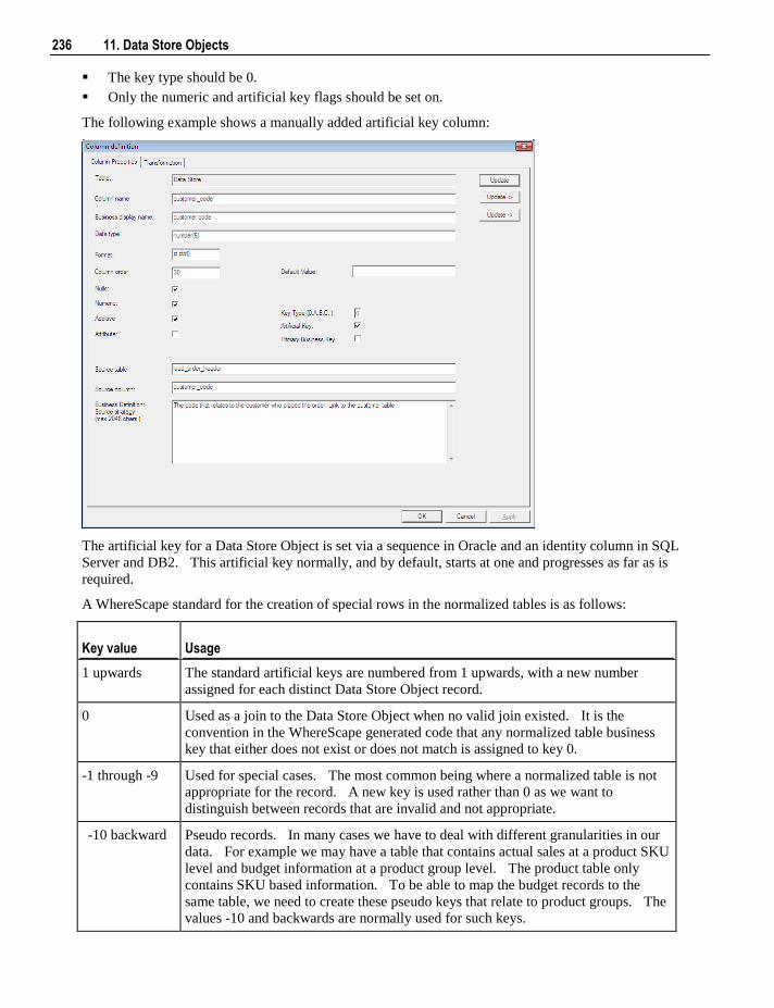
236 11. Data Store Objects
The key type should be 0.
Only the numeric and artificial key flags should be set on.
The following example shows a manually added artificial key column:
The artificial key for a Data Store Object is set via a sequence in Oracle and an identity column in SQL
Server and DB2. This artificial key normally, and by default, starts at one and progresses as far as is
required.
A WhereScape standard for the creation of special rows in the normalized tables is as follows:
Key value Usage
1 upwards The standard artificial keys are numbered from 1 upwards, with a new number
assigned for each distinct Data Store Object record.
0 Used as a join to the Data Store Object when no valid join existed. It is the
convention in the WhereScape generated code that any normalized table business
key that either does not exist or does not match is assigned to key 0.
-1 through -9 Used for special cases. The most common being where a normalized table is not
appropriate for the record. A new key is used rather than 0 as we want to
distinguish between records that are invalid and not appropriate.
-10 backward Pseudo records. In many cases we have to deal with different granularities in our
data. For example we may have a table that contains actual sales at a product SKU
level and budget information at a product group level. The product table only
contains SKU based information. To be able to map the budget records to the
same table, we need to create these pseudo keys that relate to product groups. The
values -10 and backwards are normally used for such keys.
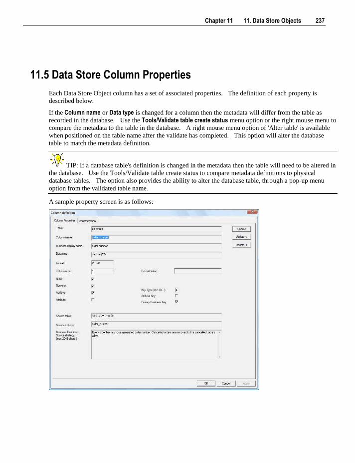
Chapter 11 11. Data Store Objects 237
11.5 Data Store Column Properties
Each Data Store Object column has a set of associated properties. The definition of each property is
described below:
If the Column name or Data type is changed for a column then the metadata will differ from the table as
recorded in the database. Use the Tools/Validate table create status menu option or the right mouse menu to
compare the metadata to the table in the database. A right mouse menu option of 'Alter table' is available
when positioned on the table name after the validate has completed. This option will alter the database
table to match the metadata definition.
TIP: If a database table's definition is changed in the metadata then the table will need to be altered in
the database. Use the Tools/Validate table create status to compare metadata definitions to physical
database tables. The option also provides the ability to alter the database table, through a pop-up menu
option from the validated table name.
A sample property screen is as follows:
238 11. Data Store Objects
The two special update keys allow you to update the column and step either forward or backward to the
next column's properties. ALT-Left Arrow and ALT-Right Arrow can also be used instead of the two special
update keys.
Table
The table to which the column belongs. Read only.
Column name
The database name of the column. This name must conform to database column naming standards.
Typically such standards exclude the use of spaces etc. A good practice is to only use alphanumerics, and
the underscore character. Changing this field alters the table's definition.
Business display name
This defines how the business refers to this column. It does not affect the physical table definition, but
rather provides input to the documentation and to the view ws_admin_v_dim_col which can be used to assist
in the population of an end user tool's end user layer. As such it is a free form entry and any characters are
valid.
Data type
This is the database specific data type. It must be a valid data type for the data warehouse database
platform. Typical data types for DB2 are integer, numeric, char(), varchar() and date. Typical data types
for Oracle are integer, number, char(), varchar2() and date. For SQL Server common types are integer,
numeric, varchar() and datetime. See the database documentation for a description of the data types
available. Changing this field alters the table's definition.
Format
This field is to allow the definition of a format mask for end user tools. It does not affect the physical table
definition, but rather provides input to the view ws_admin_v_dim_col which can be used to assist in the
population of an end user tool's end user layer. As such it is a free form entry and any characters are valid.
Typically format masks are only used on numeric fields. Example: #,###0.00. It is not worth the effort of
populating this field unless it can be utilized by the end user tools in use.
Column order
This numeric field provides the ordering of the columns in the database table create statement. The lowest
numbered column will appear first in the table. Although this affects the physical table definition no action
will be taken unless the table is re-created in the database. The columns can be re-numbered based on the
existing order by choosing the 'Respace order number' pop-up menu option when positioned over any
column in the table. This action will number the columns in increments of 10 starting at 10. In addition to
a simple change of the order field, the column order can be changed by first displaying the columns in the
middle pane and then using drag and drop to move the columns around. This drag and drop process will
automatically renumber the columns as required.
Nulls
This check box when set allows nulls to exist in this column. If cleared then nulls are not permitted in the
column.

Chapter 11 11. Data Store Objects 239
Numeric
This check box indicates that the column in question is numeric when set. This is normally only relevant
for fact tables. It does not affect the physical table definition, but rather provides input to the view
ws_admin_v_dim_col which can be used to assist in the population of an end user tool's end user layer. The
use of this field is not relevant unless it can be utilized by the end user tools.
Additive
This check box indicates that the column in question is additive when set. This implies that the column can
be summed when performing data grouping in a query. This is normally only relevant for fact tables. It
does not affect the physical table definition, but rather provides input to the view ws_admin_v_dim_col which can be used to assist in the population of an end user tool's end user layer. The use of this field is
not relevant unless it can be utilized by the end user tools.
Attribute
This checkbox indicates that the column in question is an attribute when set. An attribute is defined as a
column that is non factual. For example we may have an order number, or an invoice number stored in the
fact table. Such columns are considered attributes, rather than facts. This checkbox is therefore normally
only relevant for fact tables. This checkbox does not affect the physical table definition, but rather
provides input to the view ws_admin_v_dim_col which can be used to assist in the population of an end user
tools end user layer. The use of this field is not relevant unless it can be utilized by the end user tools.
Source table
Indicates the table from which the column was sourced. This source table is normally a load table within
the data warehouse. If the column was sourced from multiple tables, then the normal practice is to record
one of the tables in this field and a comment listing all of the other tables in the 'Source strategy' field.
This field is used when generating a procedure to update the Data Store Object. It is also used in the track
back diagrams and in the documentation.
Source column
Indicates the column in the 'Source table' from which the column was sourced. Such a column is normally
a load table column, which in turn may have been a transformation or the combination of multiple columns.
For previous value managed columns the source column is the column in the table whose previous value is
being recorded.
Business definition / Source strategy
Normally this field will contain a business definition of the column. Such a definition may be a description
of the column from a business user's point of view. This field might additionally contain information on
where and how the column was acquired. For example if the column is sourced from multiple tables or is a
composite or derived column then this definition would normally describe the process used to populate the
column. This field is used in the documentation and is available via the view ws_admin_v_dim_col . This
field is also stored as a comment against the column in the database.
Default Value
This field contains the default value applied to the column if it is not explicitly specified when the table has
data inserted into it.
240 11. Data Store Objects
Key Type
The key type is used internally by WhereScape RED in the building of the update procedure and the
generation of indexes. It can be altered here, but this should only be done if the consequences are fully
understood and tested. The supported values are:
Key type Meaning
0 The artificial key. Set when the key is added during drag and drop table
generation.
1 Component of all business keys. Indicates that this column is used as part of any
business key.
A Indicates that the column is part of the primary business key. Set whenever a
business key is defined as part of an update procedure generation.
B-Z Indicates that the column is part of a secondary business key. Only used during
index generation and not normally set.
Artificial Key
This checkbox indicates that the column is the artificial key when set. Only one artificial key is supported.
This indicator is set by WhereScape RED during the initial drag and drop creation of a table, and should not
normally be altered.
Primary Business Key
This checkbox indicates that the column is part of the primary business key when set. Multiple columns
can form the primary business key. This indicator is set and cleared by WhereScape RED during the Data
Store Object update procedure generation process. This check box should not normally be altered.
11.6 Data Store Object Column Transformations
Each Data Store Object column can have a transformation associated with it. The transformation will be
included in the generated procedure and will be executed as part of the procedure update. The
transformation must therefore be a valid SQL construct that can be included in a 'Select' statement. For
example we could have a transformation of 'load_order_line.qty * 0.125' to calculate a tax column of
12.5%. Click the 'Transformation' tab to enter a transformation.
Note: transformations are only put into effect when the procedure is re-generated.
Chapter 12 12. Normalized Tables 241
In This Chapter
12.1 Normalized Tables Overview ............................................. 242
12.2 Building a Normalized Table .............................................. 244
12.3 Generating the Normalized Update Procedure .................... 248
12.4 Normalized Table Artificial Keys ....................................... 260
12.5 Normalized Table Column Properties ................................. 263
12.6 Normalized Table Column Transformations ....................... 267
C H A P T E R 1 2
12. Normalized Tables
242 12. Normalized Tables
12.1 Normalized Tables Overview
A Normalized Table is a data warehouse object used to build third normal form enterprise data warehouses.
In WhereScape RED, normalized objects have many of the code generating attributes of stage, dimension
and fact tables. Third normal form enterprise data warehouses can be thought of as a source system for star
schema data marts. Alternatively, they may be reported off directly by users and reporting tools.
Normalized Tables can be considered either reference or transactional in nature.
A Normalized Table is built from the Data Warehouse connection. Unless you are retrofitting an existing
system, Normalized Tables are typically built from one or more load or stage tables. The normalized
model may be retrofitted from an enterprise modelling tool. See Importing a Data Model (see "30.2
Importing a Data Model" on page 680) for more details.
The usual steps for creating a normalized model are defined below and are covered in this chapter. The
steps are:
Identify the source reference or transactional data that will constitute the Normalized Table. If the
data is sourced from multiple tables ascertain if a join between the source tables is possible, or if one or
more intermediate stage (work) tables would be a better option.
Using the 'drag and drop' functionality drag the load or stage table that is the primary source of
information for the Normalized Table into a normalized target. See Building a Normalized Table (see
"12.2 Building a Normalized Table" on page 244).
If there's only one source table and all of the columns from it are being used, you can select the auto
create option to build and load the table. This automatically completes the next four steps. See
Building a Normalized Table (see "12.2 Building a Normalized Table" on page 244).
Add columns from other load and/or stage tables if required. See Building a Normalized Table (see
"12.2 Building a Normalized Table" on page 244).
Create the Normalized Table in the database. See Building a Normalized Table (see "12.2 Building a
Normalized Table" on page 244).
Build the update procedure. See Generating the Update Procedure (see "12.3 Generating the
Normalized Update Procedure" on page 248).
Run the update procedure and analyze the results.
If necessary, modify the update procedure or create a custom procedure.
Normalized Table Keys
Normalized Tables have two types of keys that we will refer to frequently. These are the Business Key and
the Artificial Key. A definition of these two key types follows:
Business Key
The business key is the column or columns that uniquely identify a record within a Normalized Table.
Where the Normalized Table maps back to a single or a main table in the source system, it is usually
possible to ascertain the business key by looking at the unique keys for that source table. The business key
is sometimes referred to as the 'natural' key. Examples of business keys are:
The product SKU in a product table
The customer code in a customer table
The IATA airport code in an airport table.
Chapter 12 12. Normalized Tables 243
It is assumed that business keys will never be NULL. If a null value is possible in a business key then the
generated code will need to be modified to handle the null value by assigning some default value. In the
following examples, the business key column is modified by using a database function and default value:
DB2: COALESCE(business_key,'N/A')
SQL Server: ISNULL(business_key,'N/A')
Oracle: NVL(business_key,'N/A')
Note: Business keys are assumed to never be Null. If they can be null it is best to transform them to some
value prior to the normalized or stage table update. If this is not done, an un-modified update procedure
will probably fail with a duplicate key error on the business key index.
Artificial Key
By default, Normalized Tables in WhereScape RED do not have an artificial key (artificial keys can be
added manually, see Normalized Table Artificial Keys (see "12.4 Normalized Table Artificial Keys" on
page 260) for more details).
An artificial key is the unique identifier that can be used to join a Normalized Table record to other
Normalized Tables. When joining Normalized Tables it would be possible to perform the join using the
business key. For Normalized Tables that satisfy one of more of the following conditions, joining with
business keys could result in slow query times and excessive use of database storage:
Multiple column business keys (excessive storage and multiple column joins)
One or more large character business key columns (excessive storage)
Very large tables (excessive storage - integer artificial keys often use less space than one small
character field)
History Normalized Tables (complex joins involving a between dates construct)
As query time is one of our key drivers in data warehouse implementations the best answer is often to use
some form of artificial key. A price is paid in the additional processing required doing key lookups, but
this is offset by the reduced query times and reduced complexity.
The artificial key is an integer and is built sequentially from 1 upwards. See the section on artificial keys
for a more detailed explanation. An artificial key is sometimes referred to as a "surrogate" key.
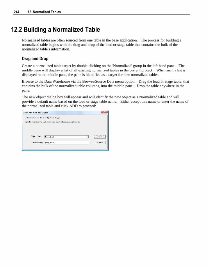
244 12. Normalized Tables
12.2 Building a Normalized Table
Normalized tables are often sourced from one table in the base application. The process for building a
normalized table begins with the drag and drop of the load or stage table that contains the bulk of the
normalized table's information.
Drag and Drop
Create a normalized table target by double clicking on the 'Normalized' group in the left hand pane. The
middle pane will display a list of all existing normalized tables in the current project. When such a list is
displayed in the middle pane, the pane is identified as a target for new normalized tables.
Browse to the Data Warehouse via the Browse/Source Data menu option. Drag the load or stage table, that
contains the bulk of the normalized table columns, into the middle pane. Drop the table anywhere in the
pane.
The new object dialog box will appear and will identify the new object as a Normalized table and will
provide a default name based on the load or stage table name. Either accept this name or enter the name of
the normalized table and click ADD to proceed:
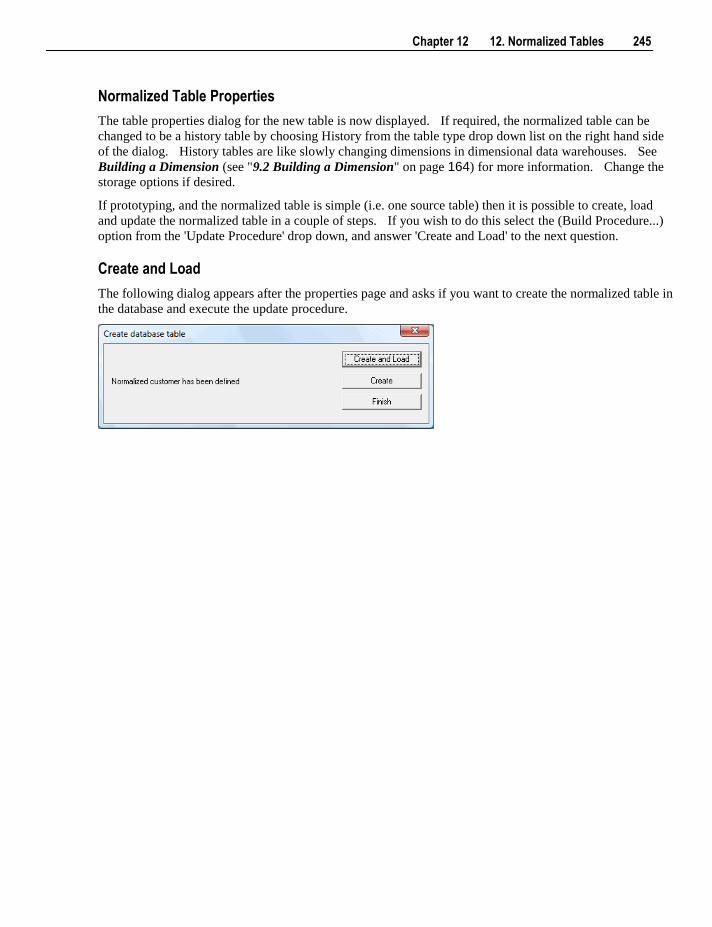
Chapter 12 12. Normalized Tables 245
Normalized Table Properties
The table properties dialog for the new table is now displayed. If required, the normalized table can be
changed to be a history table by choosing History from the table type drop down list on the right hand side
of the dialog. History tables are like slowly changing dimensions in dimensional data warehouses. See
Building a Dimension (see "9.2 Building a Dimension" on page 164) for more information. Change the
storage options if desired.
If prototyping, and the normalized table is simple (i.e. one source table) then it is possible to create, load
and update the normalized table in a couple of steps. If you wish to do this select the (Build Procedure...)
option from the 'Update Procedure' drop down, and answer 'Create and Load' to the next question.
Create and Load
The following dialog appears after the properties page and asks if you want to create the normalized table in
the database and execute the update procedure.
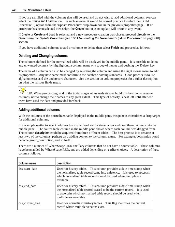
246 12. Normalized Tables
If you are satisfied with the columns that will be used and do not wish to add additional columns you can
select the Create and Load button. In such an event it would be normal practice to select the (Build
Procedure...) option from the 'Update Procedure' drop down box in the previous properties page. If no
procedure has been selected then select the Create button as no update will occur in any event.
If Create or Create and Load is selected and a new procedure creation was chosen proceed directly to the
Generating the Update Procedure (see "12.3 Generating the Normalized Update Procedure" on page 248)
section.
If you have additional columns to add or columns to delete then select Finish and proceed as follows.
Deleting and Changing columns
The columns defined for the normalized table will be displayed in the middle pane. It is possible to delete
any unwanted columns by highlighting a column name or a group of names and pushing the 'Delete' key.
The name of a column can also be changed by selecting the column and using the right mouse menu to edit
its properties. Any new name must conform to the database naming standards. Good practice is to use
alphanumerics and the underscore character. See the section on column properties for a fuller description
on what the various fields mean.
TIP: When prototyping, and in the initial stages of an analysis area build it is best not to remove
columns, nor to change their names to any great extent. This type of activity is best left until after end
users have used the data and provided feedback.
Adding additional columns
With the columns of the normalized table displayed in the middle pane, this pane is considered a drop target
for additional columns.
It is a simple matter to select columns from other load and/or stage tables and drag these columns into the
middle pane. The source table column in the middle pane shows where each column was dragged from.
The column description could be acquired from three different tables. The best practise is to rename at
least two of the columns, perhaps also adding context to the column name. For example, description could
become group_description, and so forth.
There are a number of WhereScape RED ancillary columns that do not have a source table. These columns
have been added by WhereScape RED, and are added depending on earlier choices. A description of these
columns follows.
Column name description
dss_start_date Used for history tables. This column provides a date time stamp when
the normalized table record came into existence. It is used to ascertain
which normalized table record should be used when multiple are
available.
dss_end_date Used for history tables. This column provides a date time stamp when
the normalized table record ceased to be the current record. It is used
to ascertain which normalized table record should be used when
multiple are available.
dss_current_flag Used for normalized history tables. This flag identifies the current
record where multiple versions exist.
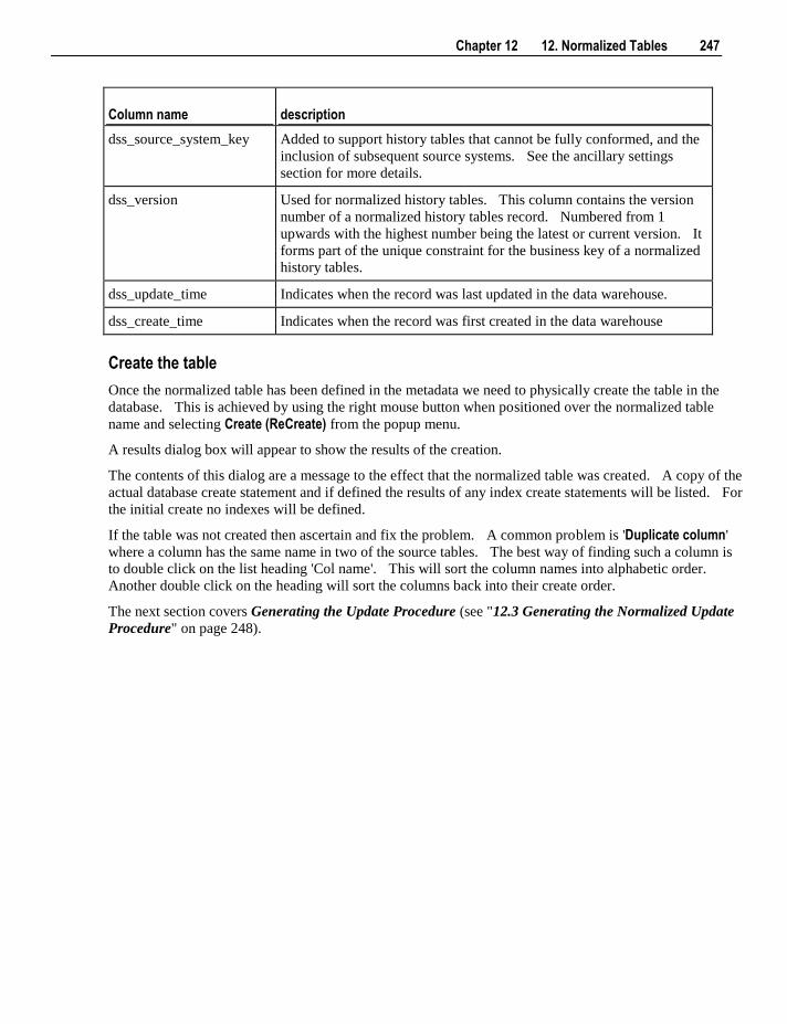
Chapter 12 12. Normalized Tables 247
Column name description
dss_source_system_key Added to support history tables that cannot be fully conformed, and the
inclusion of subsequent source systems. See the ancillary settings
section for more details.
dss_version Used for normalized history tables. This column contains the version
number of a normalized history tables record. Numbered from 1
upwards with the highest number being the latest or current version. It
forms part of the unique constraint for the business key of a normalized
history tables.
dss_update_time Indicates when the record was last updated in the data warehouse.
dss_create_time Indicates when the record was first created in the data warehouse
Create the table
Once the normalized table has been defined in the metadata we need to physically create the table in the
database. This is achieved by using the right mouse button when positioned over the normalized table
name and selecting Create (ReCreate) from the popup menu.
A results dialog box will appear to show the results of the creation.
The contents of this dialog are a message to the effect that the normalized table was created. A copy of the
actual database create statement and if defined the results of any index create statements will be listed. For
the initial create no indexes will be defined.
If the table was not created then ascertain and fix the problem. A common problem is 'Duplicate column'
where a column has the same name in two of the source tables. The best way of finding such a column is
to double click on the list heading 'Col name'. This will sort the column names into alphabetic order.
Another double click on the heading will sort the columns back into their create order.
The next section covers Generating the Update Procedure (see "12.3 Generating the Normalized Update
Procedure" on page 248).
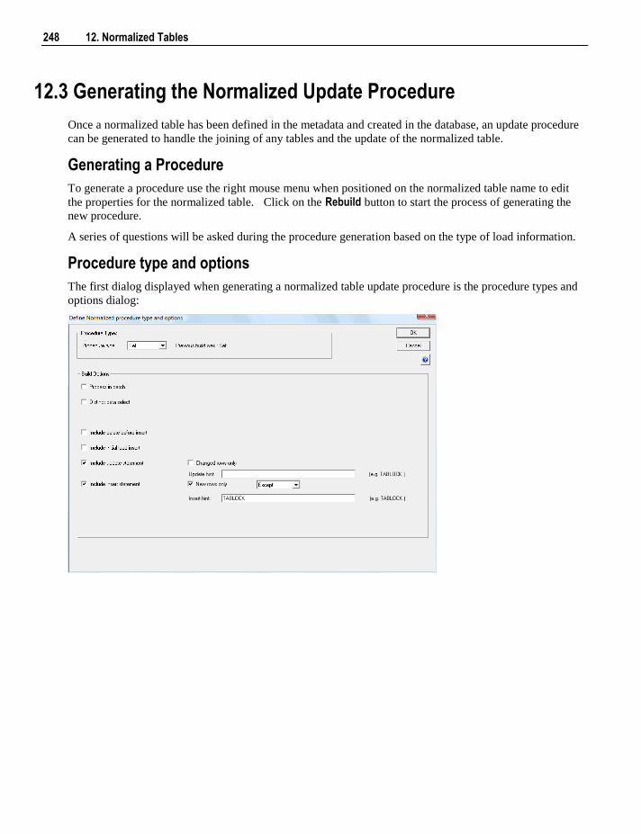
248 12. Normalized Tables
12.3 Generating the Normalized Update Procedure
Once a normalized table has been defined in the metadata and created in the database, an update procedure
can be generated to handle the joining of any tables and the update of the normalized table.
Generating a Procedure
To generate a procedure use the right mouse menu when positioned on the normalized table name to edit
the properties for the normalized table. Click on the Rebuild button to start the process of generating the
new procedure.
A series of questions will be asked during the procedure generation based on the type of load information.
Procedure type and options
The first dialog displayed when generating a normalized table update procedure is the procedure types and
options dialog:
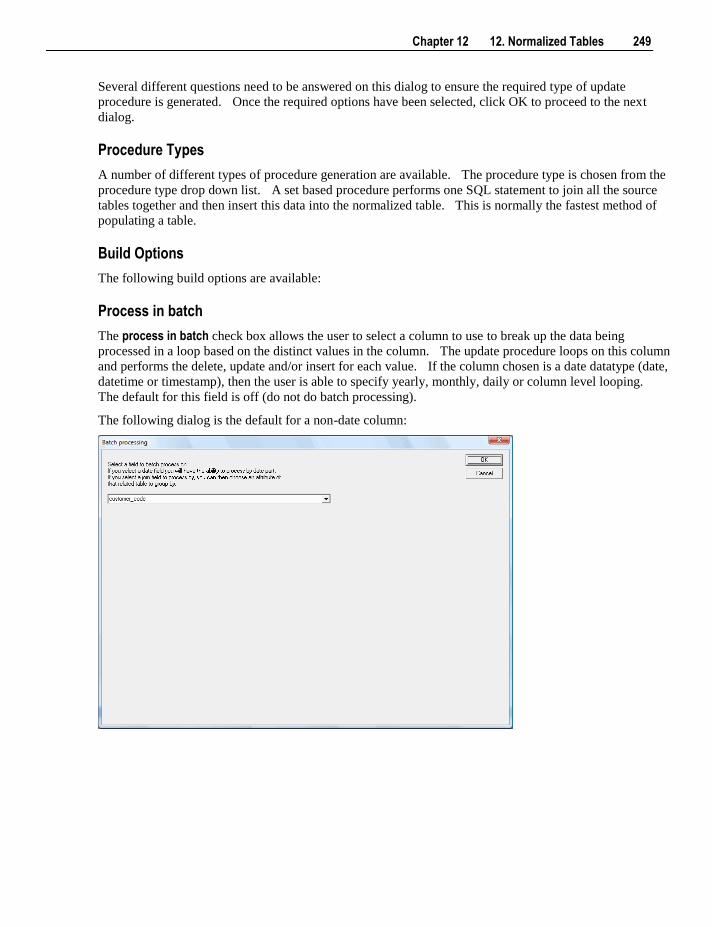
Chapter 12 12. Normalized Tables 249
Several different questions need to be answered on this dialog to ensure the required type of update
procedure is generated. Once the required options have been selected, click OK to proceed to the next
dialog.
Procedure Types
A number of different types of procedure generation are available. The procedure type is chosen from the
procedure type drop down list. A set based procedure performs one SQL statement to join all the source
tables together and then insert this data into the normalized table. This is normally the fastest method of
populating a table.
Build Options
The following build options are available:
Process in batch
The process in batch check box allows the user to select a column to use to break up the data being
processed in a loop based on the distinct values in the column. The update procedure loops on this column
and performs the delete, update and/or insert for each value. If the column chosen is a date datatype (date,
datetime or timestamp), then the user is able to specify yearly, monthly, daily or column level looping.
The default for this field is off (do not do batch processing).
The following dialog is the default for a non-date column:
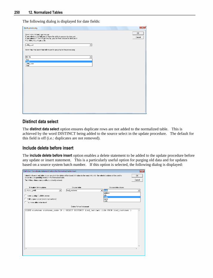
250 12. Normalized Tables
The following dialog is displayed for date fields:
Distinct data select
The distinct data select option ensures duplicate rows are not added to the normalized table. This is
achieved by the word DISTINCT being added to the source select in the update procedure. The default for
this field is off (i.e.: duplicates are not removed).
Include delete before insert
The include delete before insert option enables a delete statement to be added to the update procedure before
any update or insert statement. This is a particularly useful option for purging old data and for updates
based on a source system batch number. If this option is selected, the following dialog is displayed:
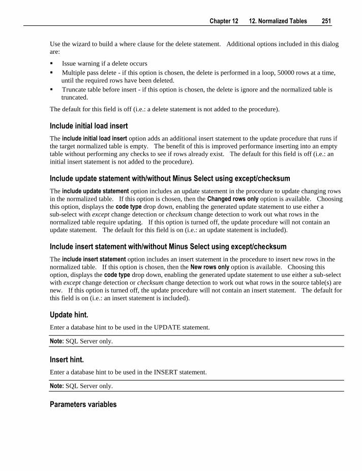
Chapter 12 12. Normalized Tables 251
Use the wizard to build a where clause for the delete statement. Additional options included in this dialog
are:
Issue warning if a delete occurs
Multiple pass delete - if this option is chosen, the delete is performed in a loop, 50000 rows at a time,
until the required rows have been deleted.
Truncate table before insert - if this option is chosen, the delete is ignore and the normalized table is
truncated.
The default for this field is off (i.e.: a delete statement is not added to the procedure).
Include initial load insert
The include initial load insert option adds an additional insert statement to the update procedure that runs if
the target normalized table is empty. The benefit of this is improved performance inserting into an empty
table without performing any checks to see if rows already exist. The default for this field is off (i.e.: an
initial insert statement is not added to the procedure).
Include update statement with/without Minus Select using except/checksum
The include update statement option includes an update statement in the procedure to update changing rows
in the normalized table. If this option is chosen, then the Changed rows only option is available. Choosing
this option, displays the code type drop down, enabling the generated update statement to use either a
sub-select with except change detection or checksum change detection to work out what rows in the
normalized table require updating. If this option is turned off, the update procedure will not contain an
update statement. The default for this field is on (i.e.: an update statement is included).
Include insert statement with/without Minus Select using except/checksum
The include insert statement option includes an insert statement in the procedure to insert new rows in the
normalized table. If this option is chosen, then the New rows only option is available. Choosing this
option, displays the code type drop down, enabling the generated update statement to use either a sub-select
with except change detection or checksum change detection to work out what rows in the source table(s) are
new. If this option is turned off, the update procedure will not contain an insert statement. The default for
this field is on (i.e.: an insert statement is included).
Update hint.
Enter a database hint to be used in the UPDATE statement.
Note: SQL Server only.
Insert hint.
Enter a database hint to be used in the INSERT statement.
Note: SQL Server only.
Parameters variables

252 12. Normalized Tables
If WhereScape RED parameters exist in the metadata, the following dialog is displayed. Any parameters
selected in this dialog (by moving them to the left hand side), are included in the generated update
procedure as variables. The procedure will include code to retrieve the value of the parameter at run time
and store it in the declared variable.
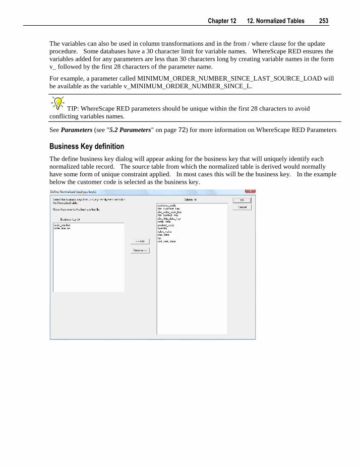
Chapter 12 12. Normalized Tables 253
The variables can also be used in column transformations and in the from / where clause for the update
procedure. Some databases have a 30 character limit for variable names. WhereScape RED ensures the
variables added for any parameters are less than 30 characters long by creating variable names in the form
v_ followed by the first 28 characters of the parameter name.
For example, a parameter called MINIMUM_ORDER_NUMBER_SINCE_LAST_SOURCE_LOAD will
be available as the variable v_MINIMUM_ORDER_NUMBER_SINCE_L.
TIP: WhereScape RED parameters should be unique within the first 28 characters to avoid
conflicting variables names.
See Parameters (see "5.2 Parameters" on page 72) for more information on WhereScape RED Parameters
Business Key definition
The define business key dialog will appear asking for the business key that will uniquely identify each
normalized table record. The source table from which the normalized table is derived would normally
have some form of unique constraint applied. In most cases this will be the business key. In the example
below the customer code is selected as the business key.
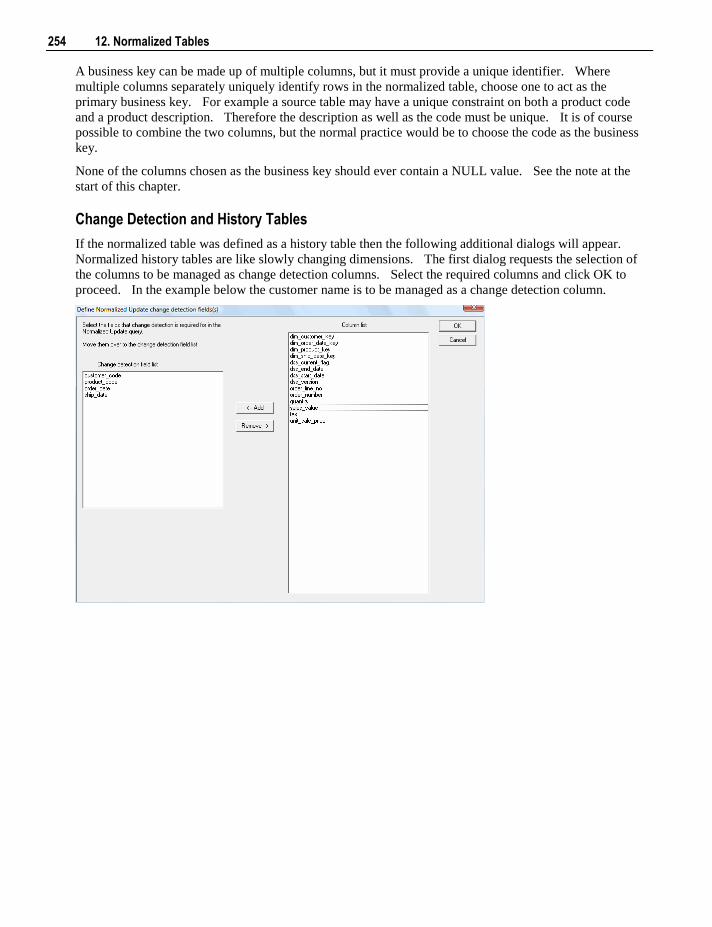
254 12. Normalized Tables
A business key can be made up of multiple columns, but it must provide a unique identifier. Where
multiple columns separately uniquely identify rows in the normalized table, choose one to act as the
primary business key. For example a source table may have a unique constraint on both a product code
and a product description. Therefore the description as well as the code must be unique. It is of course
possible to combine the two columns, but the normal practice would be to choose the code as the business
key.
None of the columns chosen as the business key should ever contain a NULL value. See the note at the
start of this chapter.
Change Detection and History Tables
If the normalized table was defined as a history table then the following additional dialogs will appear.
Normalized history tables are like slowly changing dimensions. The first dialog requests the selection of
the columns to be managed as change detection columns. Select the required columns and click OK to
proceed. In the example below the customer name is to be managed as a change detection column.
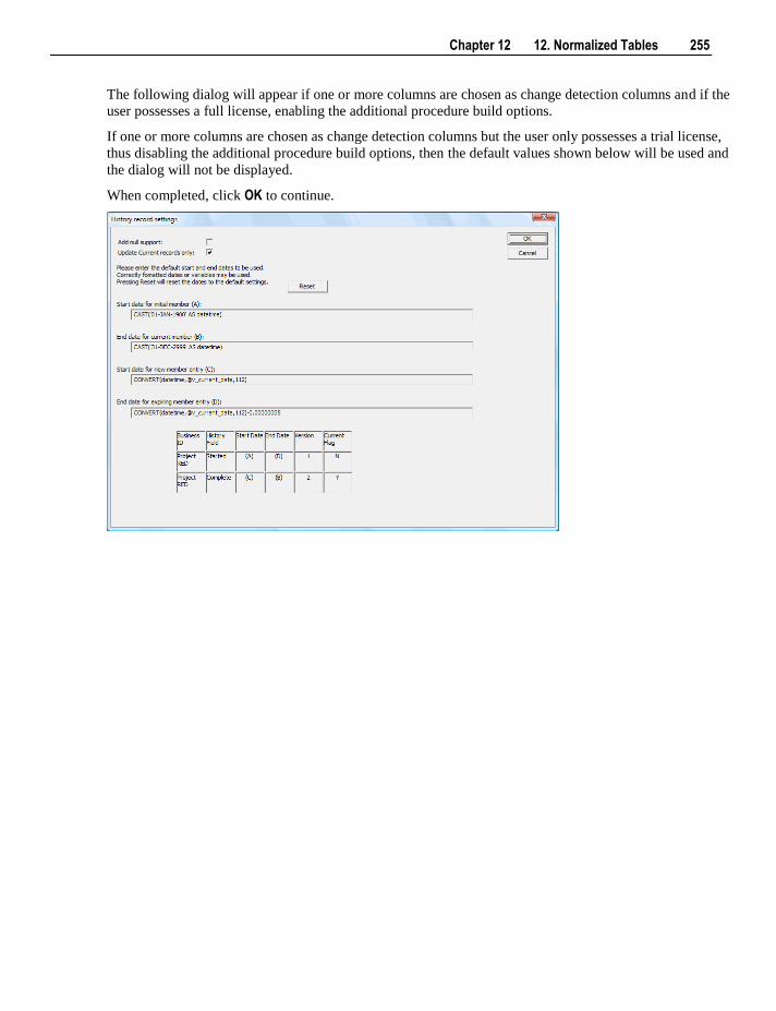
Chapter 12 12. Normalized Tables 255
The following dialog will appear if one or more columns are chosen as change detection columns and if the
user possesses a full license, enabling the additional procedure build options.
If one or more columns are chosen as change detection columns but the user only possesses a trial license,
thus disabling the additional procedure build options, then the default values shown below will be used and
the dialog will not be displayed.
When completed, click OK to continue.
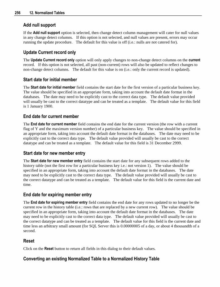
256 12. Normalized Tables
Add null support
If the Add null support option is selected, then change detect column management will cater for null values
in any change detect columns. If this option is not selected, and null values are present, errors may occur
running the update procedure. The default for this value is off (i.e.: nulls are not catered for).
Update Current record only
The Update Current record only option will only apply changes to non-change detect columns on the current record. If this option is not selected, all past (non-current) rows will also be updated to reflect changes to
non-change detect columns. The default for this value is on (i.e.: only the current record is updated).
Start date for initial member
The Start date for initial member field contains the start date for the first version of a particular business key.
The value should be specified in an appropriate form, taking into account the default date format in the
databases. The date may need to be explicitly cast to the correct data type. The default value provided
will usually be cast to the correct datatype and can be treated as a template. The default value for this field
is 1 January 1900.
End date for current member
The End date for current member field contains the end date for the current version (the row with a current
flag of Y and the maximum version number) of a particular business key. The value should be specified in
an appropriate form, taking into account the default date format in the databases. The date may need to be
explicitly cast to the correct data type. The default value provided will usually be cast to the correct
datatype and can be treated as a template. The default value for this field is 31 December 2999.
Start date for new member entry
The Start date for new member entry field contains the start date for any subsequent rows added to the
history table (not the first row for a particular business key i.e.: not version 1). The value should be
specified in an appropriate form, taking into account the default date format in the databases. The date
may need to be explicitly cast to the correct data type. The default value provided will usually be cast to
the correct datatype and can be treated as a template. The default value for this field is the current date and
time.
End date for expiring member entry
The End date for expiring member entry field contains the end date for any rows updated to no longer be the
current row in the history table (i.e.: rows that are replaced by a new current row). The value should be
specified in an appropriate form, taking into account the default date format in the databases. The date
may need to be explicitly cast to the correct data type. The default value provided will usually be cast to
the correct datatype and can be treated as a template. The default value for this field is the current date and
time less an arbitrary small amount (for SQL Server this is 0.00000005 of a day, or about 4 thousandth of a
second.
Reset
Click on the Reset button to return all fields in this dialog to their default values.
Converting an existing Normalized Table to a Normalized History Table
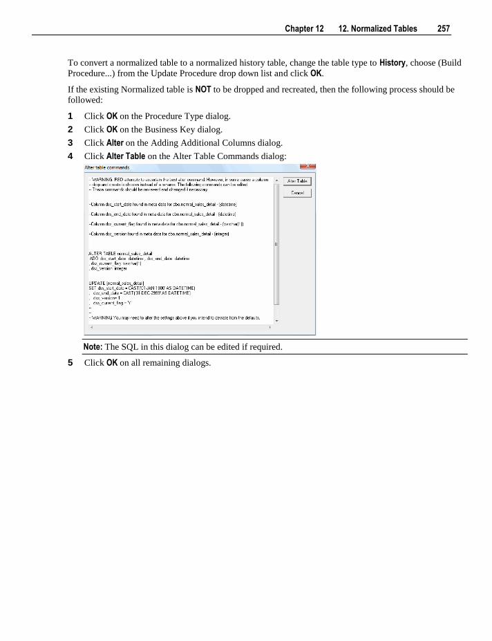
Chapter 12 12. Normalized Tables 257
To convert a normalized table to a normalized history table, change the table type to History, choose (Build
Procedure...) from the Update Procedure drop down list and click OK.
If the existing Normalized table is NOT to be dropped and recreated, then the following process should be
followed:
1 Click OK on the Procedure Type dialog.
2 Click OK on the Business Key dialog.
3 Click Alter on the Adding Additional Columns dialog.
4 Click Alter Table on the Alter Table Commands dialog:
Note: The SQL in this dialog can be edited if required.
5 Click OK on all remaining dialogs.
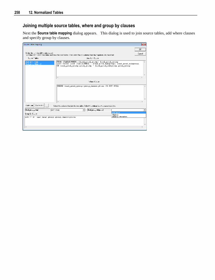
258 12. Normalized Tables
Joining multiple source tables, where and group by clauses
Next the Source table mapping dialog appears. This dialog is used to join source tables, add where clauses
and specify group by clauses.
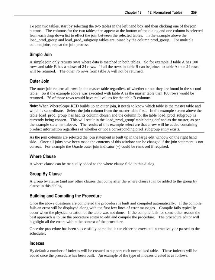
Chapter 12 12. Normalized Tables 259
To join two tables, start by selecting the two tables in the left hand box and then clicking one of the join
buttons. The columns for the two tables then appear at the bottom of the dialog and one column is selected
from each drop down list to effect the join between the selected tables. In the example above the
load_prod_group and load_prod_subgroup tables are joined by the column prod_group. For multiple
column joins, repeat the join process.
Simple Join
A simple join only returns rows where data is matched in both tables. So for example if table A has 100
rows and table B has a subset of 24 rows. If all the rows in table B can be joined to table A then 24 rows
will be returned. The other 76 rows from table A will not be returned.
Outer Join
The outer join returns all rows in the master table regardless of whether or not they are found in the second
table. So if the example above was executed with table A as the master table then 100 rows would be
returned. 76 of those rows would have null values for the table B columns.
Note: When WhereScape RED builds up an outer join, it needs to know which table is the master table and
which is subordinate. Select the join column from the master table first. In the example screen above the
table 'load_prod_group' has had its column chosen and the column for the table 'load_prod_subgroup' is
currently being chosen. This will result in the 'load_prod_group' table being defined as the master, as per
the example statement above. The results of this example select are that a row will be added containing
product information regardless of whether or not a corresponding prod_subgroup entry exists.
As the join columns are selected the join statement is built up in the large edit window on the right hand
side. Once all joins have been made the contents of this window can be changed if the join statement is not
correct. For example the Oracle outer join indicator (+) could be removed if required.
Where Clause
A where clause can be manually added to the where clause field in this dialog.
Group By Clause
A group by clause (and any other clauses that come after the where clause) can be added to the group by
clause in this dialog.
Building and Compiling the Procedure
Once the above questions are completed the procedure is built and compiled automatically. If the compile
fails an error will be displayed along with the first few lines of error messages. Compile fails typically
occur when the physical creation of the table was not done. If the compile fails for some other reason the
best approach is to use the procedure editor to edit and compile the procedure. The procedure editor will
highlight all the errors within the context of the procedure.
Once the procedure has been successfully compiled it can either be executed interactively or passed to the
scheduler.
Indexes
By default a number of indexes will be created to support each normalized table. These indexes will be
added once the procedure has been built. An example of the type of indexes created is as follows:
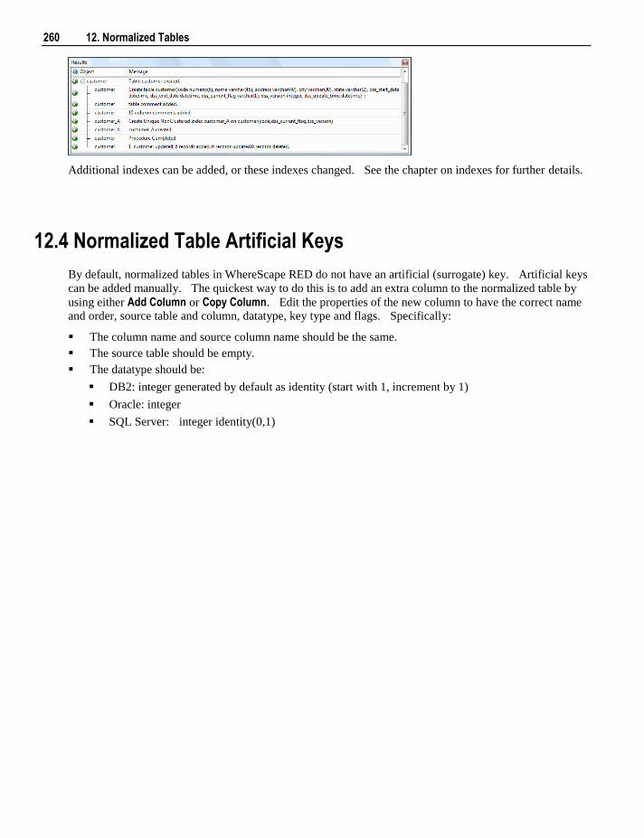
260 12. Normalized Tables
Additional indexes can be added, or these indexes changed. See the chapter on indexes for further details.
12.4 Normalized Table Artificial Keys
By default, normalized tables in WhereScape RED do not have an artificial (surrogate) key. Artificial keys
can be added manually. The quickest way to do this is to add an extra column to the normalized table by
using either Add Column or Copy Column. Edit the properties of the new column to have the correct name
and order, source table and column, datatype, key type and flags. Specifically:
The column name and source column name should be the same.
The source table should be empty.
The datatype should be:
DB2: integer generated by default as identity (start with 1, increment by 1)
Oracle: integer
SQL Server: integer identity(0,1)
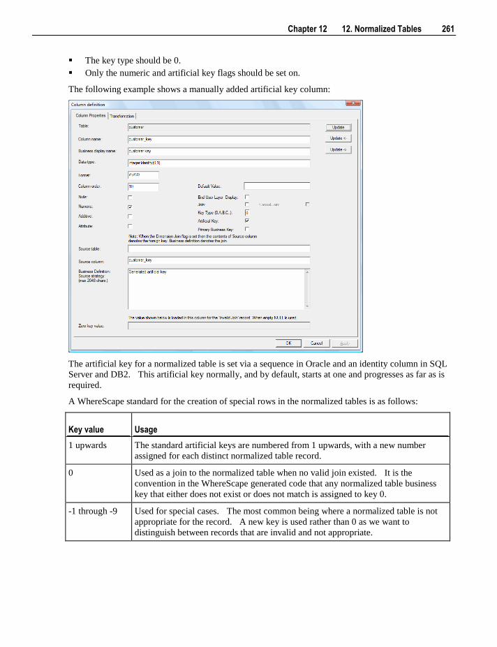
Chapter 12 12. Normalized Tables 261
The key type should be 0.
Only the numeric and artificial key flags should be set on.
The following example shows a manually added artificial key column:
The artificial key for a normalized table is set via a sequence in Oracle and an identity column in SQL
Server and DB2. This artificial key normally, and by default, starts at one and progresses as far as is
required.
A WhereScape standard for the creation of special rows in the normalized tables is as follows:
Key value Usage
1 upwards The standard artificial keys are numbered from 1 upwards, with a new number
assigned for each distinct normalized table record.
0 Used as a join to the normalized table when no valid join existed. It is the
convention in the WhereScape generated code that any normalized table business
key that either does not exist or does not match is assigned to key 0.
-1 through -9 Used for special cases. The most common being where a normalized table is not
appropriate for the record. A new key is used rather than 0 as we want to
distinguish between records that are invalid and not appropriate.
262 12. Normalized Tables
Key value Usage
-10 backward Pseudo records. In many cases we have to deal with different granularities in our
data. For example we may have a table that contains actual sales at a product SKU
level and budget information at a product group level. The product table only
contains SKU based information. To be able to map the budget records to the
same table, we need to create these pseudo keys that relate to product groups. The
values -10 and backwards are normally used for such keys.
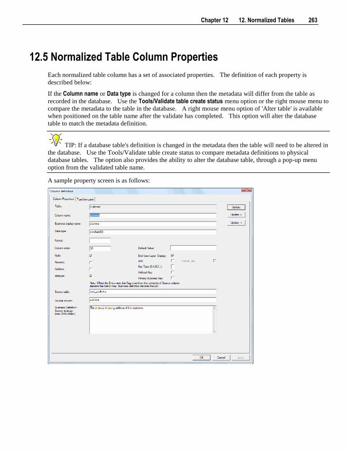
Chapter 12 12. Normalized Tables 263
12.5 Normalized Table Column Properties
Each normalized table column has a set of associated properties. The definition of each property is
described below:
If the Column name or Data type is changed for a column then the metadata will differ from the table as
recorded in the database. Use the Tools/Validate table create status menu option or the right mouse menu to
compare the metadata to the table in the database. A right mouse menu option of 'Alter table' is available
when positioned on the table name after the validate has completed. This option will alter the database
table to match the metadata definition.
TIP: If a database table's definition is changed in the metadata then the table will need to be altered in
the database. Use the Tools/Validate table create status to compare metadata definitions to physical
database tables. The option also provides the ability to alter the database table, through a pop-up menu
option from the validated table name.
A sample property screen is as follows:

264 12. Normalized Tables
The two special update keys allow you to update the column and step either forward or backward to the
next column's properties. ALT-Left Arrow and ALT-Right Arrow can also be used instead of the two special
update keys.
Table
The table to which the column belongs. Read only.
Column name
The database name of the column. This name must conform to database column naming standards.
Typically such standards exclude the use of spaces etc. A good practice is to only use alphanumerics, and
the underscore character. Changing this field alters the table's definition.
Business display name
This defines how the business refers to this column. It does not affect the physical table definition, but
rather provides input to the documentation and to the view ws_admin_v_dim_col which can be used to assist
in the population of an end user tool's end user layer. As such it is a free form entry and any characters are
valid.
Data type
This is the database specific data type. It must be a valid data type for the data warehouse database
platform. Typical data types for DB2 are integer, numeric, char(), varchar() and date. Typical data types
for Oracle are integer, number, char(), varchar2() and date. For SQL Server common types are integer,
numeric, varchar() and datetime. See the database documentation for a description of the data types
available. Changing this field alters the table's definition.
Format
This field is to allow the definition of a format mask for end user tools. It does not affect the physical table
definition, but rather provides input to the view ws_admin_v_dim_col which can be used to assist in the
population of an end user tool's end user layer. As such it is a free form entry and any characters are valid.
Typically format masks are only used on numeric fields. Example: #,###0.00. It is not worth the effort of
populating this field unless it can be utilized by the end user tools in use.
Column order
This numeric field provides the ordering of the columns in the database table create statement. The lowest
numbered column will appear first in the table. Although this affects the physical table definition no action
will be taken unless the table is re-created in the database. The columns can be re-numbered based on the
existing order by choosing the 'Respace order number' pop-up menu option when positioned over any
column in the table. This action will number the columns in increments of 10 starting at 10. In addition to
a simple change of the order field, the column order can be changed by first displaying the columns in the
middle pane and then using drag and drop to move the columns around. This drag and drop process will
automatically renumber the columns as required.
Nulls
This check box when set allows nulls to exist in this column. If cleared then nulls are not permitted in the
column.
Chapter 12 12. Normalized Tables 265
Numeric
This check box indicates that the column in question is numeric when set. This is normally only relevant
for fact tables. It does not affect the physical table definition, but rather provides input to the view
ws_admin_v_dim_col which can be used to assist in the population of an end user tool's end user layer. The
use of this field is not relevant unless it can be utilized by the end user tools.
Additive
This check box indicates that the column in question is additive when set. This implies that the column can
be summed when performing data grouping in a query. This is normally only relevant for fact tables. It
does not affect the physical table definition, but rather provides input to the view ws_admin_v_dim_col which can be used to assist in the population of an end user tool's end user layer. The use of this field is
not relevant unless it can be utilized by the end user tools.
Attribute
This checkbox indicates that the column in question is an attribute when set. An attribute is defined as a
column that is non factual. For example we may have an order number, or an invoice number stored in the
fact table. Such columns are considered attributes, rather than facts. This checkbox is therefore normally
only relevant for fact tables. This checkbox does not affect the physical table definition, but rather
provides input to the view ws_admin_v_dim_col which can be used to assist in the population of an end user
tools end user layer. The use of this field is not relevant unless it can be utilized by the end user tools.
Source table
Indicates the table from which the column was sourced. This source table is normally a load table within
the data warehouse. If the column was sourced from multiple tables, then the normal practice is to record
one of the tables in this field and a comment listing all of the other tables in the 'Source strategy' field.
This field is used when generating a procedure to update the normalized table. It is also used in the track
back diagrams and in the documentation.
Source column
Indicates the column in the 'Source table' from which the column was sourced. Such a column is normally
a load table column, which in turn may have been a transformation or the combination of multiple columns.
For previous value managed columns the source column is the column in the table whose previous value is
being recorded.
Business definition / Source strategy
Normally this field will contain a business definition of the column. Such a definition may be a description
of the column from a business user's point of view. This field might additionally contain information on
where and how the column was acquired. For example if the column is sourced from multiple tables or is a
composite or derived column then this definition would normally describe the process used to populate the
column. This field is used in the documentation and is available via the view ws_admin_v_dim_col . This
field is also stored as a comment against the column in the database.
Default Value
This field contains the default value applied to the column if it is not explicitly specified when the table has
data inserted into it.
266 12. Normalized Tables
End User Layer display
This checkbox when set indicates that the column is intended for end user view. If set the documentation
will include the column in the glossary and in the user documentation. It is also used to decide what
columns appear in the view ws_admin_v_dim_col. Typically columns such as the artificial key would not
be enabled for end user display.
Join
This checkbox is set by WhereScape RED during the building of the update procedure and should not
normally be altered. It indicates that the column in question provides a join to another normalized table.
The 'Source table' and 'Source column' fields will provide the other normalized table's side of the join.
Manual Join
This checkbox can be set to change the way the other normalized table is looked up during the update
procedure build. Enabling this option allows you to join to the normalized table manually during the
procedure build process. The usual dialog for matching the other normalized table business key to a
column or columns in the table is not displayed if this option is enabled.
Key Type
The key type is used internally by WhereScape RED in the building of the update procedure and the
generation of indexes. It can be altered here, but this should only be done if the consequences are fully
understood and tested. The supported values are:
Key type Meaning
0 The artificial key. Set when the key is added during drag and drop table
generation.
1 Component of all business keys. Indicates that this column is used as part of any
business key.
A Indicates that the column is part of the primary business key. Set whenever a
business key is defined as part of an update procedure generation.
B-Z Indicates that the column is part of a secondary business key. Only used during
index generation and not normally set.
Artificial Key
This checkbox indicates that the column is the artificial key when set. Only one artificial key is supported.
This indicator is set by WhereScape RED during the initial drag and drop creation of a table, and should not
normally be altered.
Primary Business Key
This checkbox indicates that the column is part of the primary business key when set. Multiple columns
can form the primary business key. This indicator is set and cleared by WhereScape RED during the
normalized table update procedure generation process. This checkbox should not normally be altered.
Chapter 12 12. Normalized Tables 267
12.6 Normalized Table Column Transformations
Each normalized table column can have a transformation associated with it. The transformation will be
included in the generated procedure and will be executed as part of the procedure update. The
transformation must therefore be a valid SQL construct that can be included in a 'Select' statement. For
example we could have a transformation of 'load_order_line.qty * 0.125' to calculate a tax column of 12.5%
Click the 'Transformation' tab to enter a transformation.
Note: transformations are only put into effect when the procedure is re-generated.

Chapter 13 13. Fact Tables 269
A Fact Table is normally defined, for our purposes, as a table with facts (measures) and dimensional keys
that allow the linking of multiple dimensions. It is normally illustrated in the form of a Star Schema with
the central fact table and the outlying dimensions.
The ultimate goal of the Fact Table is to provide business information to the end user community. In many
cases, different types of fact table are required to address different end user requirements. For simplicity
the different types of fact table will be grouped together under the following headings:
Detail (see "13.1 Detail Fact Tables" on page 270)
Rollup (see "13.2 Rollup or Combined Fact Tables" on page 271)
KPI (see "13.3 KPI Fact Tables" on page 273)
Snapshot (see "13.4 Snapshot Fact Tables" on page 281) (essentially a type of Rollup fact table)
Slowly Changing (see "13.5 Slowly Changing Fact Tables" on page 281)
Partitioned (see "13.6 Partitioned Fact Tables" on page 282)
In This Chapter
13.1 Detail Fact Tables ............................................................... 270
13.2 Rollup or Combined Fact Tables ......................................... 271
13.3 KPI Fact Tables ................................................................... 273
13.4 Snapshot Fact Tables ........................................................... 281
13.5 Slowly Changing Fact Tables.............................................. 281
13.6 Partitioned Fact Tables ........................................................ 282
13.7 Fact Table Column Properties ............................................. 295
13.8 Fact Table Language Mapping ............................................ 299
C H A P T E R 1 3
13. Fact Tables
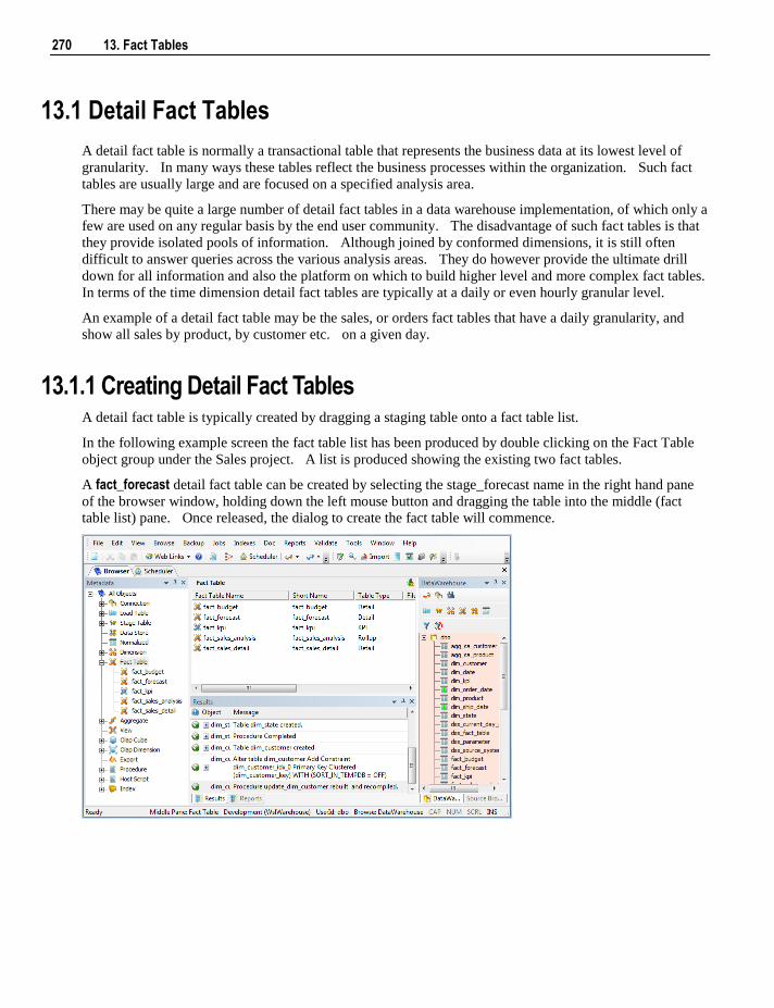
270 13. Fact Tables
13.1 Detail Fact Tables
A detail fact table is normally a transactional table that represents the business data at its lowest level of
granularity. In many ways these tables reflect the business processes within the organization. Such fact
tables are usually large and are focused on a specified analysis area.
There may be quite a large number of detail fact tables in a data warehouse implementation, of which only a
few are used on any regular basis by the end user community. The disadvantage of such fact tables is that
they provide isolated pools of information. Although joined by conformed dimensions, it is still often
difficult to answer queries across the various analysis areas. They do however provide the ultimate drill
down for all information and also the platform on which to build higher level and more complex fact tables.
In terms of the time dimension detail fact tables are typically at a daily or even hourly granular level.
An example of a detail fact table may be the sales, or orders fact tables that have a daily granularity, and
show all sales by product, by customer etc. on a given day.
13.1.1 Creating Detail Fact Tables A detail fact table is typically created by dragging a staging table onto a fact table list.
In the following example screen the fact table list has been produced by double clicking on the Fact Table
object group under the Sales project. A list is produced showing the existing two fact tables.
A fact_forecast detail fact table can be created by selecting the stage_forecast name in the right hand pane
of the browser window, holding down the left mouse button and dragging the table into the middle (fact
table list) pane. Once released, the dialog to create the fact table will commence.
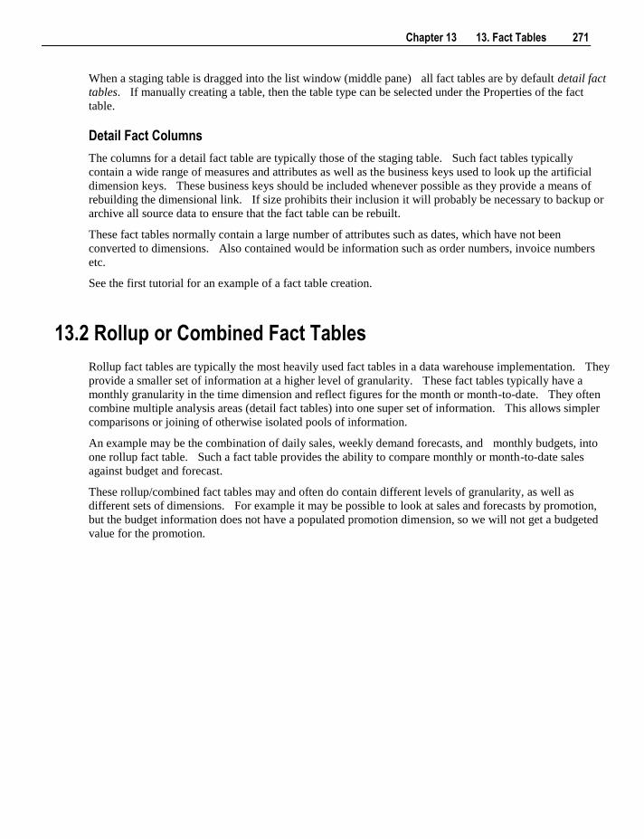
Chapter 13 13. Fact Tables 271
When a staging table is dragged into the list window (middle pane) all fact tables are by default detail fact
tables. If manually creating a table, then the table type can be selected under the Properties of the fact
table.
Detail Fact Columns
The columns for a detail fact table are typically those of the staging table. Such fact tables typically
contain a wide range of measures and attributes as well as the business keys used to look up the artificial
dimension keys. These business keys should be included whenever possible as they provide a means of
rebuilding the dimensional link. If size prohibits their inclusion it will probably be necessary to backup or
archive all source data to ensure that the fact table can be rebuilt.
These fact tables normally contain a large number of attributes such as dates, which have not been
converted to dimensions. Also contained would be information such as order numbers, invoice numbers
etc.
See the first tutorial for an example of a fact table creation.
13.2 Rollup or Combined Fact Tables
Rollup fact tables are typically the most heavily used fact tables in a data warehouse implementation. They
provide a smaller set of information at a higher level of granularity. These fact tables typically have a
monthly granularity in the time dimension and reflect figures for the month or month-to-date. They often
combine multiple analysis areas (detail fact tables) into one super set of information. This allows simpler
comparisons or joining of otherwise isolated pools of information.
An example may be the combination of daily sales, weekly demand forecasts, and monthly budgets, into
one rollup fact table. Such a fact table provides the ability to compare monthly or month-to-date sales
against budget and forecast.
These rollup/combined fact tables may and often do contain different levels of granularity, as well as
different sets of dimensions. For example it may be possible to look at sales and forecasts by promotion,
but the budget information does not have a populated promotion dimension, so we will not get a budgeted
value for the promotion.
272 13. Fact Tables
13.2.1 Creating Rollup Fact Tables A rollup or combined fact table is typically created by dragging a fact table onto a fact table list. In the
example screenshot below a double click on the Fact Table object group under the Sales project produced a
list in the middle pane showing the existing fact tables. A fact_sales_analysis rollup fact table is being
created after having selected the fact_sales_detail table in the right hand panel, holding down the left mouse
button and dragging the table into the middle pane. The initial object create dialog will appear. Note that
the name implies that this is a rollup fact table. The name will be changed to the one chosen above. A list
of columns is displayed and those not required are deleted (everything except additive measures and
dimensions).
Drag and drop additional columns from other fact tables into the middle pane if required. Where columns
have the same name these will need to be changed. For example if we acquired a quantity column from
fact_sales_detail and a column of the same name from fact_forecast we may choose to change the names to
actual_quantity and forecast_quantity.
Once all columns have been defined:
1 create the table
2 edit the properties of the table and request that a new procedure be created.
Once OK is entered the dialog to create a template procedure will commence. Included in this process will
be the definition of the date dimension granularity. Monthly rollup is the norm. To just combine fact
tables with no rollup select the date dimension key as directed in the dialog. Other forms of dimension
rollup will require some alteration to the produced template procedure.
Rollup Fact Columns
The columns for a rollup fact table are typically the dimensions, and only those key measures that are
added. For example in the sales world, measures may simply be quantity, kilograms, $value,
forecast_quantity, forecast_$value, budget_quantity, budget_$value.
See the second tutorial for an example of rollup fact table creation.

Chapter 13 13. Fact Tables 273
13.3 KPI Fact Tables
Key Performance Indicator (KPI) fact tables share a lot of similarities with the rollup fact tables in that they
are typically at a monthly level of granularity and they combine information from multiple detail fact tables.
They differ in that they provide specific sets of pre-defined information (KPIs). Such KPIs are often
difficult to answer and require the implementation of some form of business rule. Also they often provide
pre-calculated year-to-date, same month last year, and previous year-to-date values for easier comparisons.
They will have a KPI dimension which provides a list of all the specific statistics or performance indicators
we are tracking.
An example from our previous sales examples may be a set of KPIs dealing with customer acquisition and
loss. We may have a specific KPI that records the number of new customers during the period and the
$value of their business during that period. Another KPI may record the percentage growth of all
customers over the last six months. Another may show the number of customers who closed their accounts
in the period, and the value of their business over the preceding 12 months.
KPI fact tables require the specific definition of each KPI.
It is strongly recommended that the KPI tutorial be undertaken. This tutorial will give an understanding of
what can be achieved via a KPI fact table.
13.3.1 Creating the KPI Dimension The KPI dimension essentially provides a record of each KPI or statistic we are tracking. There should be
one row in this table for each such element. The KPI fact table requires that this dimension contain at the
least an artificial dimension key and a business key. We will refer to the business key as the KPI Identifier.
The following example covers the manual creation of a basic KPI dimension:
1 When positioned over the Dimension object group use the right mouse menu and select the 'New Object' menu option.
2 Give the new dimension a name for example dim_kpi.
3 Select a Normal dimension and click OK on the properties screen to define the dimension table.
4 Position on the dimension name in the left hand pane and using the right mouse menu to 'Add Column',
add the three columns defined in the following table.
Field Column 1 Column 2 Column 3
Column Name dim_kpi_key kpi_identifier kpi_name
Business display kpi artificial key kpi unique id kpi name
Datatype
- Oracle
- SQL Server / DB2
integer
integer
varchar2(12)
varchar(12)
varchar2(256)
varchar(256)
Nulls Clear Clear Checked
Key Type 0 A Clear
Artificial Key Checked Clear Clear
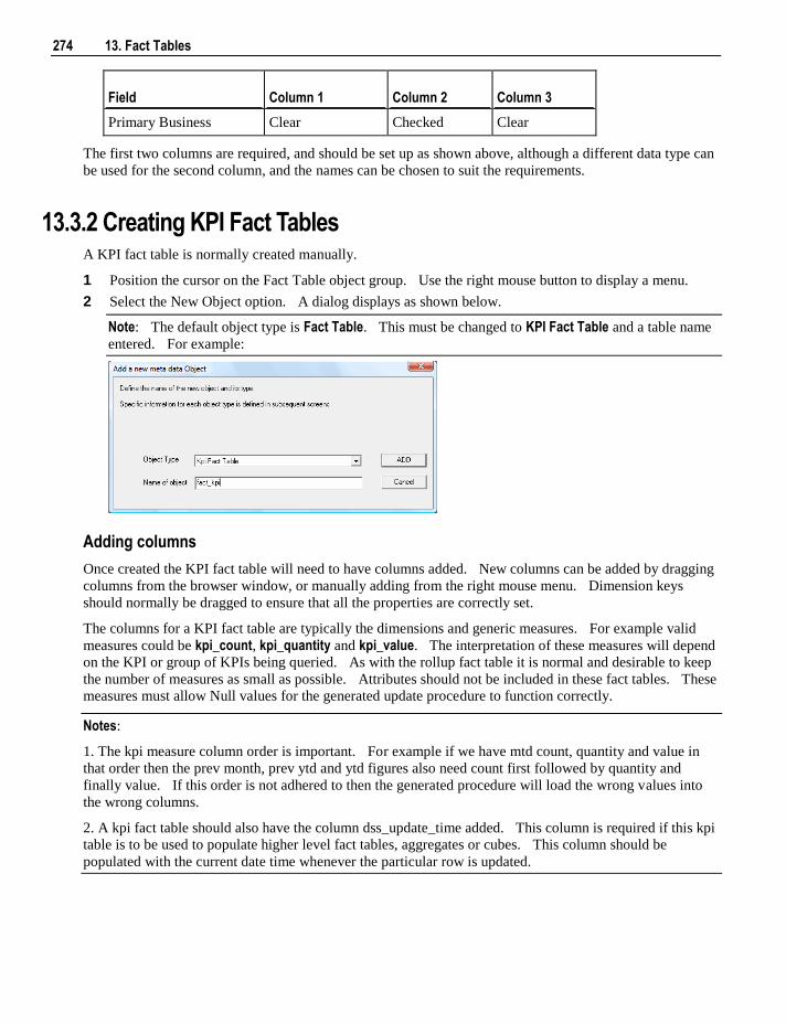
274 13. Fact Tables
Field Column 1 Column 2 Column 3
Primary Business Clear Checked Clear
The first two columns are required, and should be set up as shown above, although a different data type can
be used for the second column, and the names can be chosen to suit the requirements.
13.3.2 Creating KPI Fact Tables A KPI fact table is normally created manually.
1 Position the cursor on the Fact Table object group. Use the right mouse button to display a menu.
2 Select the New Object option. A dialog displays as shown below.
Note: The default object type is Fact Table. This must be changed to KPI Fact Table and a table name
entered. For example:
Adding columns
Once created the KPI fact table will need to have columns added. New columns can be added by dragging
columns from the browser window, or manually adding from the right mouse menu. Dimension keys
should normally be dragged to ensure that all the properties are correctly set.
The columns for a KPI fact table are typically the dimensions and generic measures. For example valid
measures could be kpi_count, kpi_quantity and kpi_value. The interpretation of these measures will depend
on the KPI or group of KPIs being queried. As with the rollup fact table it is normal and desirable to keep
the number of measures as small as possible. Attributes should not be included in these fact tables. These
measures must allow Null values for the generated update procedure to function correctly.
Notes:
1. The kpi measure column order is important. For example if we have mtd count, quantity and value in
that order then the prev month, prev ytd and ytd figures also need count first followed by quantity and
finally value. If this order is not adhered to then the generated procedure will load the wrong values into
the wrong columns.
2. A kpi fact table should also have the column dss_update_time added. This column is required if this kpi
table is to be used to populate higher level fact tables, aggregates or cubes. This column should be
populated with the current date time whenever the particular row is updated.
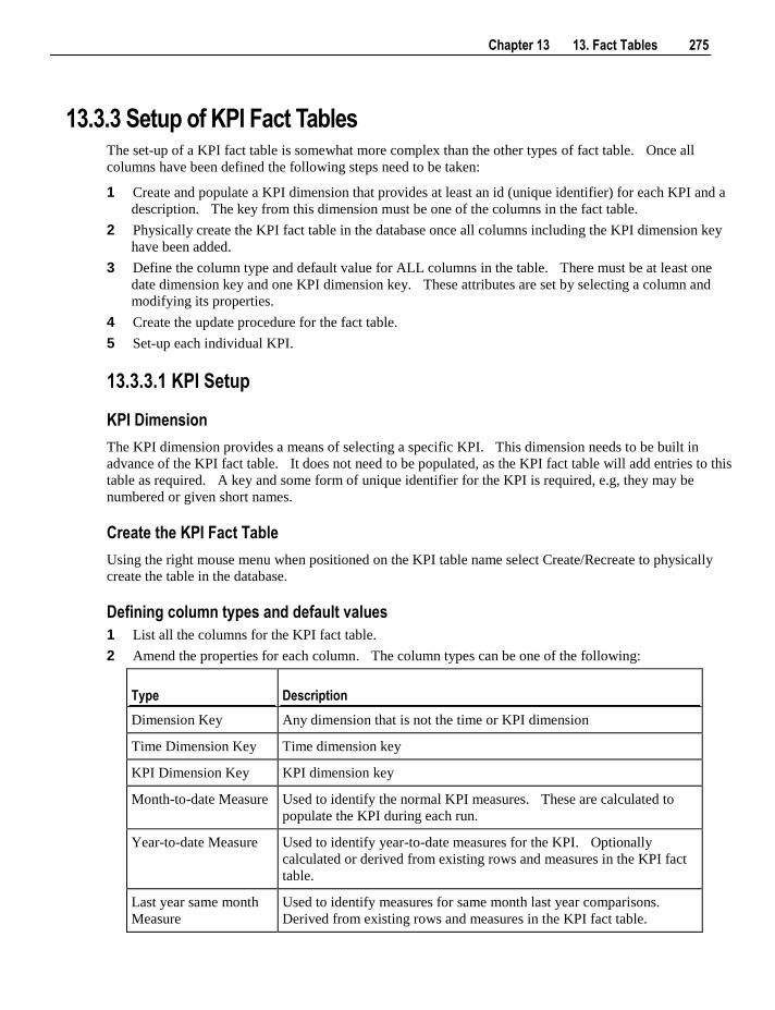
Chapter 13 13. Fact Tables 275
13.3.3 Setup of KPI Fact Tables The set-up of a KPI fact table is somewhat more complex than the other types of fact table. Once all
columns have been defined the following steps need to be taken:
1 Create and populate a KPI dimension that provides at least an id (unique identifier) for each KPI and a
description. The key from this dimension must be one of the columns in the fact table.
2 Physically create the KPI fact table in the database once all columns including the KPI dimension key
have been added.
3 Define the column type and default value for ALL columns in the table. There must be at least one
date dimension key and one KPI dimension key. These attributes are set by selecting a column and
modifying its properties.
4 Create the update procedure for the fact table.
5 Set-up each individual KPI.
13.3.3.1 KPI Setup
KPI Dimension
The KPI dimension provides a means of selecting a specific KPI. This dimension needs to be built in
advance of the KPI fact table. It does not need to be populated, as the KPI fact table will add entries to this
table as required. A key and some form of unique identifier for the KPI is required, e.g, they may be
numbered or given short names.
Create the KPI Fact Table
Using the right mouse menu when positioned on the KPI table name select Create/Recreate to physically
create the table in the database.
Defining column types and default values
1 List all the columns for the KPI fact table.
2 Amend the properties for each column. The column types can be one of the following:
Type Description
Dimension Key Any dimension that is not the time or KPI dimension
Time Dimension Key Time dimension key
KPI Dimension Key KPI dimension key
Month-to-date Measure Used to identify the normal KPI measures. These are calculated to
populate the KPI during each run.
Year-to-date Measure Used to identify year-to-date measures for the KPI. Optionally
calculated or derived from existing rows and measures in the KPI fact
table.
Last year same month
Measure
Used to identify measures for same month last year comparisons.
Derived from existing rows and measures in the KPI fact table.
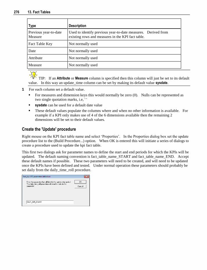
276 13. Fact Tables
Type Description
Previous year-to-date
Measure
Used to identify previous year-to-date measures. Derived from
existing rows and measures in the KPI fact table.
Fact Table Key Not normally used
Date Not normally used
Attribute Not normally used
Measure Not normally used
TIP: If an Attribute or Measure column is specified then this column will just be set to its default
value. In this way an update_time column can be set by making its default value sysdate.
1 For each column set a default value.
For measures and dimension keys this would normally be zero (0). Nulls can be represented as
two single quotation marks, i.e, ' '
sysdate can be used for a default date value
These default values populate the columns where and when no other information is available. For
example if a KPI only makes use of 4 of the 6 dimensions available then the remaining 2
dimensions will be set to their default values.
Create the 'Update' procedure
Right mouse on the KPI fact table name and select „Properties‟. In the Properties dialog box set the update
procedure list to the (Build Procedure...) option. When OK is entered this will initiate a series of dialogs to
create a procedure used to update the kpi fact table.
This first two dialogs ask for parameter names to define the start and end periods for which the KPIs will be
updated. The default naming convention is fact_table_name_START and fact_table_name_END. Accept
these default names if possible. These two parameters will need to be created, and will need to be updated
once the KPIs have been defined and tested. Under normal operation these parameters should probably be
set daily from the daily_time_roll procedure.
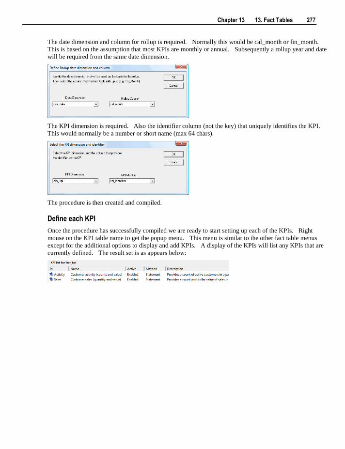
Chapter 13 13. Fact Tables 277
The date dimension and column for rollup is required. Normally this would be cal_month or fin_month.
This is based on the assumption that most KPIs are monthly or annual. Subsequently a rollup year and date
will be required from the same date dimension.
The KPI dimension is required. Also the identifier column (not the key) that uniquely identifies the KPI.
This would normally be a number or short name (max 64 chars).
The procedure is then created and compiled.
Define each KPI
Once the procedure has successfully compiled we are ready to start setting up each of the KPIs. Right
mouse on the KPI table name to get the popup menu. This menu is similar to the other fact table menus
except for the additional options to display and add KPIs. A display of the KPIs will list any KPIs that are
currently defined. The result set is as appears below:
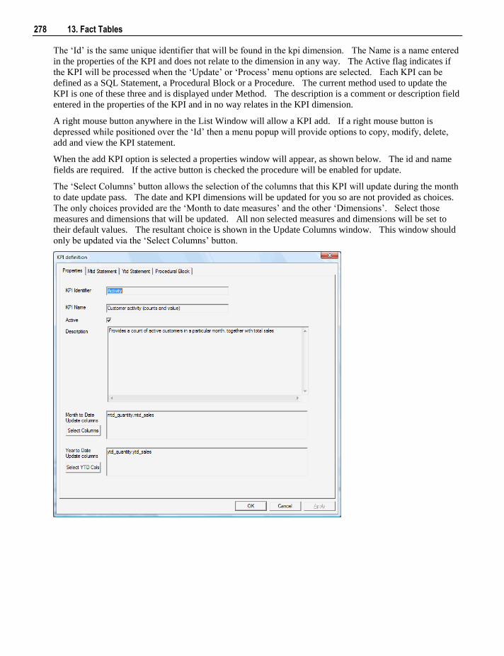
278 13. Fact Tables
The „Id‟ is the same unique identifier that will be found in the kpi dimension. The Name is a name entered
in the properties of the KPI and does not relate to the dimension in any way. The Active flag indicates if
the KPI will be processed when the „Update‟ or „Process‟ menu options are selected. Each KPI can be
defined as a SQL Statement, a Procedural Block or a Procedure. The current method used to update the
KPI is one of these three and is displayed under Method. The description is a comment or description field
entered in the properties of the KPI and in no way relates in the KPI dimension.
A right mouse button anywhere in the List Window will allow a KPI add. If a right mouse button is
depressed while positioned over the „Id‟ then a menu popup will provide options to copy, modify, delete,
add and view the KPI statement.
When the add KPI option is selected a properties window will appear, as shown below. The id and name
fields are required. If the active button is checked the procedure will be enabled for update.
The „Select Columns‟ button allows the selection of the columns that this KPI will update during the month
to date update pass. The date and KPI dimensions will be updated for you so are not provided as choices.
The only choices provided are the „Month to date measures‟ and the other „Dimensions‟. Select those
measures and dimensions that will be updated. All non selected measures and dimensions will be set to
their default values. The resultant choice is shown in the Update Columns window. This window should
only be updated via the „Select Columns‟ button.
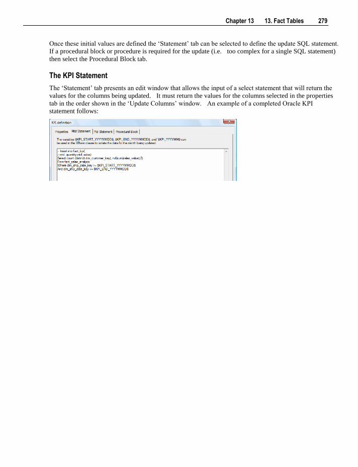
Chapter 13 13. Fact Tables 279
Once these initial values are defined the „Statement‟ tab can be selected to define the update SQL statement.
If a procedural block or procedure is required for the update (i.e. too complex for a single SQL statement)
then select the Procedural Block tab.
The KPI Statement
The „Statement‟ tab presents an edit window that allows the input of a select statement that will return the
values for the columns being updated. It must return the values for the columns selected in the properties
tab in the order shown in the „Update Columns‟ window. An example of a completed Oracle KPI
statement follows:
280 13. Fact Tables
The first two lines are comments inserted (when modifying) to provide a reminder of the columns and order
required by the select statement. Anything prior to the initial select statement is ignored.
The statement must make use of at least one of the variables provided to select the appropriate period. This
variable will be replaced with the values for the period being updated at run time. These values are derived
from the start and end parameters defined for the KPI fact table.
In order to group by the non selected columns and any attributes etc.WhereScape RED must be able to
break this statement into its component Select, From, Where, Group By, and Having components (where
present). If a complex statement is used that has more than one of these key words then the primary one
must be in UPPER case. For example if a sub query is being used then the main SELECT and FROM key
words must be in upper case and must be the only occurrence of these key words in uppercase.
WhereScape RED will check and issue a warning if it is unable to resolve the main key words.
To facilitate the testing of a statement there is a „View statement‟ option when you right mouse button on
the KPI Id. This will provide a window with the full statement with the default columns inserted and the
parameters converted. This statement can be cut and run in Sql Admin (shipped with WhereScape RED)
or in a database specific utility for testing.
Procedural Block
The „Procedural Block‟ tab presents an edit window that allows the input of an Oracle anonymous block.
If there is anything in this window it will be actioned instead of the statement. A button in the lower right
allows a rudimentary template block to be built. If used this block must do the actual insert statement
rather than just the select. It must also handle ALL dimension, month to date measure and non standard
columns. In addition, it will need to put default values in columns not actively being updated. The KPI
dimension and date dimension keys must also be updated. The output from a „View Statement‟ option for
another KPI will give an indication of what the block must do. The same month last year, year to date and
previous year to date measures will still be handled automatically. The same $KPI_ variables as shown
above the statement edit window can and must be used.
Procedure
If for some reason it is not possible to implement the KPI in either the statement or procedural block then a
procedure may be created. The name of such a procedure can be entered in the window at the bottom of
the Procedural Block tab. If any value is in this window then the procedure will take precedence over both
the statement and block.
This procedure must adhere to the standard set of parameters as with all other procedures to be executed by
the scheduler. It must undertake the same tasks as defined above in the Procedural Block section, and as
with those tasks it does not need to set the year to date, last year same month and previous year to date
values.
Copying KPIs
By choosing „copy kpi‟ from the right mouse popup menu when positioned over a KPI „Id‟ an exact
duplicate of the KPI will be inserted. This copy can then have its Id and Name changed along with its
statement to create a new KPI. This is particularly useful when only small differences exist between a
number of KPIs.
Testing / Development.
Chapter 13 13. Fact Tables 281
During testing it would be normal to DISABLE all KPIs except the one currently being developed. In this
way the update or process options will only utilize that KPI. As mentioned above the „View Statement‟
option of the KPI popup menu displays, and allows the cutting of, the statement that will be executed to
acquire the KPI information. This statement can be tested in sql*plus or some other environment if
problems are encountered.
13.4 Snapshot Fact Tables
Snapshot fact tables provide an „as at‟ view of some part of the business. They always have a time
dimension that represents the „as at‟ date. For example, we may have a weekly or monthly snapshot of our
inventory information. Such a snapshot would allow us to see what inventory we had at a particular point
in time, and allow us to compare our holdings over time. Snapshots are often used when dealing with
people profiles or client/customer profiles to enable us to view the state of our relationship with an entity at
a given point in time, e.g, to see a monthly trend of a client's outstanding balance.
13.4.1 Creating Snapshot Fact Tables The creation of snapshot fact tables is very dependent on the method used to create the snapshot. In some
cases they may be created in exactly the same way as detail fact tables. Such cases are typically where the
OLTP application provides the „as at‟ state. For example an inventory system may provide a weekly stock
take table which is the basis for our snapshot fact table. In such cases the table is created as per a detail
fact table, but with additional tailoring around the time dimension. In other situations the snapshot is built
from an existing transactional fact table, where all information up to a specific date is summarized or frozen
to create the snapshot. In these instances the snapshot can be created as a rollup fact table. Regardless of
whether a detail or rollup method is used for the creation of the snapshot table, a significant amount of work
will be required to tailor the update procedure to reflect the particular requirements of the snapshot table.
Snapshot Fact Columns
The columns for a snapshot fact table vary to a large degree. A date dimension is always present to reflect
the „as at‟ date. Some snapshots may have a large number of measures reflecting $values quantities etc,
whereas others may be rich in attribute (non additive) facts.
13.5 Slowly Changing Fact Tables
Slowly changing fact tables provide a complete history of changes for some part of the business. Typically
such fact tables are used for situations where a relatively small number of changes occur over time, but we
need to track all of these changes. A good example is an inventory stock holding that does not change very
often. In such a case a slowly changing fact table can record both the current inventory levels as well as
providing a means of seeing the state of inventory holdings at any point in time.
282 13. Fact Tables
13.5.1 Creating Slowly Changing Fact Tables WhereScape RED does not provide any automated way for creating a slowly changing fact table. The best
method is to proceed as follows.
1 Drag and drop the stage table into a dimension target and create a dummy slowly changing dimension
with the name we will be using for our fact table. (i.e. fact_...).
2 Answer the questions to the pop-up dialog boxes. Select a join if asked, but do not bother to join any
of the tables. Select the columns to be managed as slowly changing. Normally these will be the
measures such as quantity and all of the dimension keys. The generated procedure will fail to compile.
3 Inspect the additional columns added for the dimension and make a note of them. Specifically
dss_end_date, dss_start_date, dss_current_flag and dss_version.
4 Inspect the indexes created to help manage the slowly changing dimension and make a note of their
columns.
5 Delete the dummy dimension you have created.
6 Delete the get_.._key procedure created for the dimension. Do not delete the update procedure.
7 Create a detail fact table in the normal manner.
8 Add in the special columns as created for the dimension. Namely dss_end_date, dss_start_date,
dss_current_flag and dss_version.
9 Recreate the table
10 Create indexes as per the dimension table to help maintain the slowly changing fact table.
11 Modify the update procedure for the fact table. Bring up the old version of the procedure that was
created for the dimension of the same name. This will have been automatically versioned out when the
latest procedure was created and can be seen through the procedure viewer.
12 This new procedure will need to merge the code from the old procedure, which will provide a guide in
how to build the code for a slowly changing fact table.
13.6 Partitioned Fact Tables
Partitioned fact tables are normally used for performance reasons. They allow us to break a large fact table
into a number of smaller tables (partitions).
Note: Partitioned fact tables are not directly supported in SQL Server 2000. A view must be created over
a number of tables to create the concept of a logical partitioned fact table.
WhereScape RED supports partitioned fact tables. The following section explains their creation and
support.
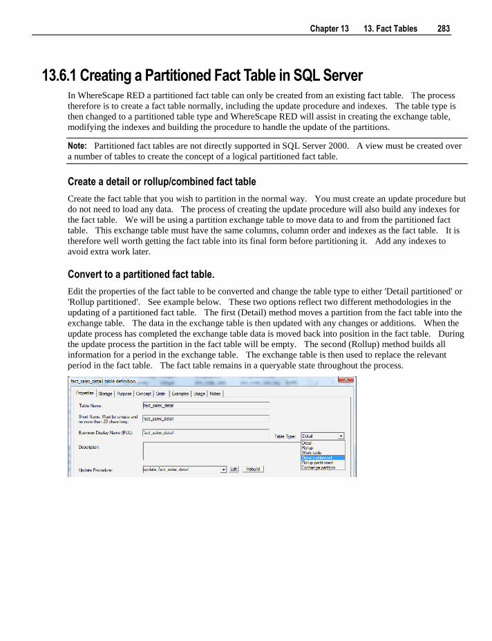
Chapter 13 13. Fact Tables 283
13.6.1 Creating a Partitioned Fact Table in SQL Server In WhereScape RED a partitioned fact table can only be created from an existing fact table. The process
therefore is to create a fact table normally, including the update procedure and indexes. The table type is
then changed to a partitioned table type and WhereScape RED will assist in creating the exchange table,
modifying the indexes and building the procedure to handle the update of the partitions.
Note: Partitioned fact tables are not directly supported in SQL Server 2000. A view must be created over
a number of tables to create the concept of a logical partitioned fact table.
Create a detail or rollup/combined fact table
Create the fact table that you wish to partition in the normal way. You must create an update procedure but
do not need to load any data. The process of creating the update procedure will also build any indexes for
the fact table. We will be using a partition exchange table to move data to and from the partitioned fact
table. This exchange table must have the same columns, column order and indexes as the fact table. It is
therefore well worth getting the fact table into its final form before partitioning it. Add any indexes to
avoid extra work later.
Convert to a partitioned fact table.
Edit the properties of the fact table to be converted and change the table type to either 'Detail partitioned' or
'Rollup partitioned'. See example below. These two options reflect two different methodologies in the
updating of a partitioned fact table. The first (Detail) method moves a partition from the fact table into the
exchange table. The data in the exchange table is then updated with any changes or additions. When the
update process has completed the exchange table data is moved back into position in the fact table. During
the update process the partition in the fact table will be empty. The second (Rollup) method builds all
information for a period in the exchange table. The exchange table is then used to replace the relevant
period in the fact table. The fact table remains in a queryable state throughout the process.

284 13. Fact Tables
A dialog will pop-up as follows, asking for confirmation that the table is to be converted to a partitioned
fact table. If 'yes' is chosen then the existing fact table will be renamed to become the partition exchange
table. Any current data will remain in this table.
The parameters for the partitioned fact table are then prompted for:
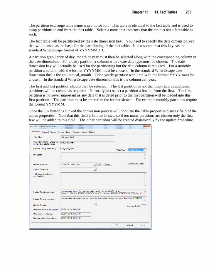
Chapter 13 13. Fact Tables 285
The partition exchange table name is prompted for. This table is identical to the fact table and is used to
swap partitions to and from the fact table. Select a name that indicates that the table is not a fact table as
such.
The fact table will be partitioned by the date dimension key. You need to specify the date dimension key
that will be used as the basis for the partitioning of the fact table. It is assumed that this key has the
standard WhereScape format of YYYYMMDD.
A partition granularity of day, month or year must then be selected along with the corresponding column in
the date dimension. For a daily partition a column with a date data type must be chosen. The date
dimension key will actually be used for the partitioning but the date column is required. For a monthly
partition a column with the format YYYYMM must be chosen. In the standard WhereScape date
dimension this is the column cal_month. For a yearly partition a column with the format YYYY must be
chosen. In the standard WhereScape date dimension this is the column cal_year.
The first and last partition should then be selected. The last partition is not that important as additional
partitions will be created as required. Normally just select a partition a few on from the first. The first
partition is however important as any data that is dated prior to the first partition will be loaded into this
first partition. The partition must be entered in the format shown. For example monthly partitions require
the format YYYYMM.
Once the OK button is clicked the conversion process will populate the 'table properties clauses' field of the
tables properties. Note that this field is limited in size, so if too many partitions are chosen only the first
few will be added to this field. The other partitions will be created dynamically by the update procedure.
286 13. Fact Tables
Click the OK button on the table properties dialog to begin the process of converting the fact table, creating
the new fact table and building the new update procedure. Examine the results screen to see what has been
done.
The partition table will now have any current data, to populate the fact table, copy the data from partition
table to the fact table, drop and recreate fact index. The date dimension key used to base the partitioning
on is not allowed to have nulls. WhereScape RED has modified the table property, however the partition
table needs to be validated and recreated to be valid. Now the fact table can be processed.
The partitioned fact table update procedure
The generated procedure will handle the creation of new partitions as required. Any data for periods prior
to the first partition is placed in the first partition. If data is received for a period after the last partition
then new partitions are created. Empty partitions are created if necessary to skip periods where no data is
present. For example, if we have a table partitioned by month and the latest partition is 200204
(april/2002). If data is then received for say september 2002 the update procedure will build partitions for
may, june, july, august and september. There is a variable at the start of the update procedure called
v_max_skip_periods. This variable is by default set to 12. This defines the maximum number of
continuous partitions we will leave empty. From our previous example if our latest partition was april
2002 and we received data for july 2003 with no interim data then the update procedure will fail as it would
have to skip 14 partitions. This check is present to prevent erroneous data from creating hundreds of
partitions into the future.
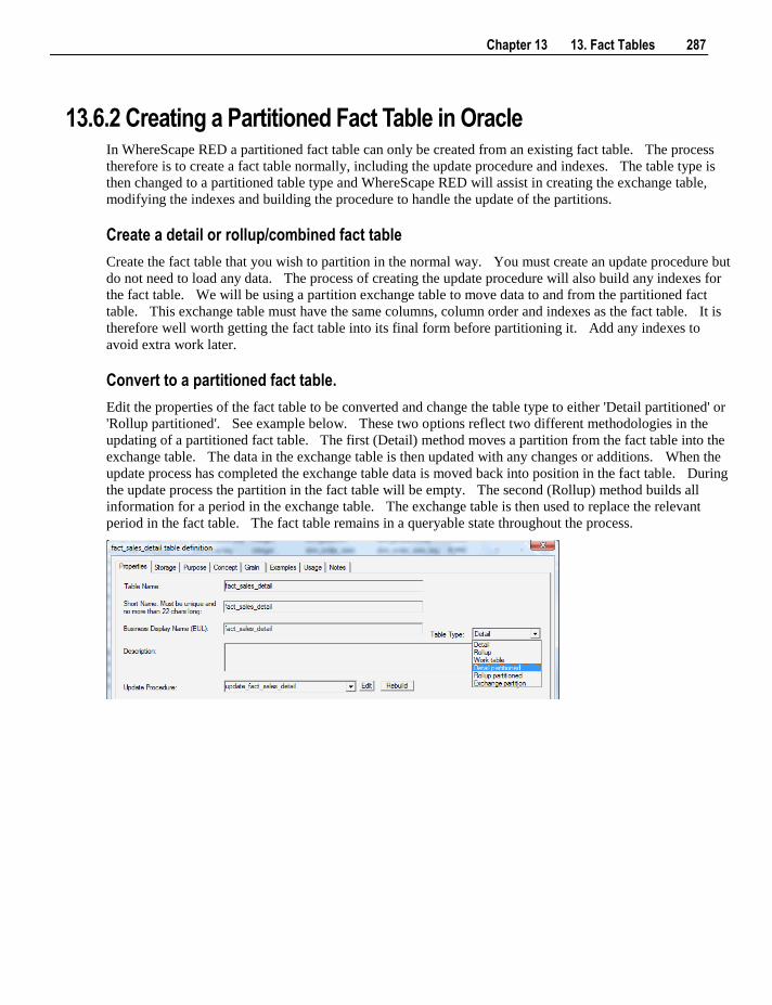
Chapter 13 13. Fact Tables 287
13.6.2 Creating a Partitioned Fact Table in Oracle In WhereScape RED a partitioned fact table can only be created from an existing fact table. The process
therefore is to create a fact table normally, including the update procedure and indexes. The table type is
then changed to a partitioned table type and WhereScape RED will assist in creating the exchange table,
modifying the indexes and building the procedure to handle the update of the partitions.
Create a detail or rollup/combined fact table
Create the fact table that you wish to partition in the normal way. You must create an update procedure but
do not need to load any data. The process of creating the update procedure will also build any indexes for
the fact table. We will be using a partition exchange table to move data to and from the partitioned fact
table. This exchange table must have the same columns, column order and indexes as the fact table. It is
therefore well worth getting the fact table into its final form before partitioning it. Add any indexes to
avoid extra work later.
Convert to a partitioned fact table.
Edit the properties of the fact table to be converted and change the table type to either 'Detail partitioned' or
'Rollup partitioned'. See example below. These two options reflect two different methodologies in the
updating of a partitioned fact table. The first (Detail) method moves a partition from the fact table into the
exchange table. The data in the exchange table is then updated with any changes or additions. When the
update process has completed the exchange table data is moved back into position in the fact table. During
the update process the partition in the fact table will be empty. The second (Rollup) method builds all
information for a period in the exchange table. The exchange table is then used to replace the relevant
period in the fact table. The fact table remains in a queryable state throughout the process.
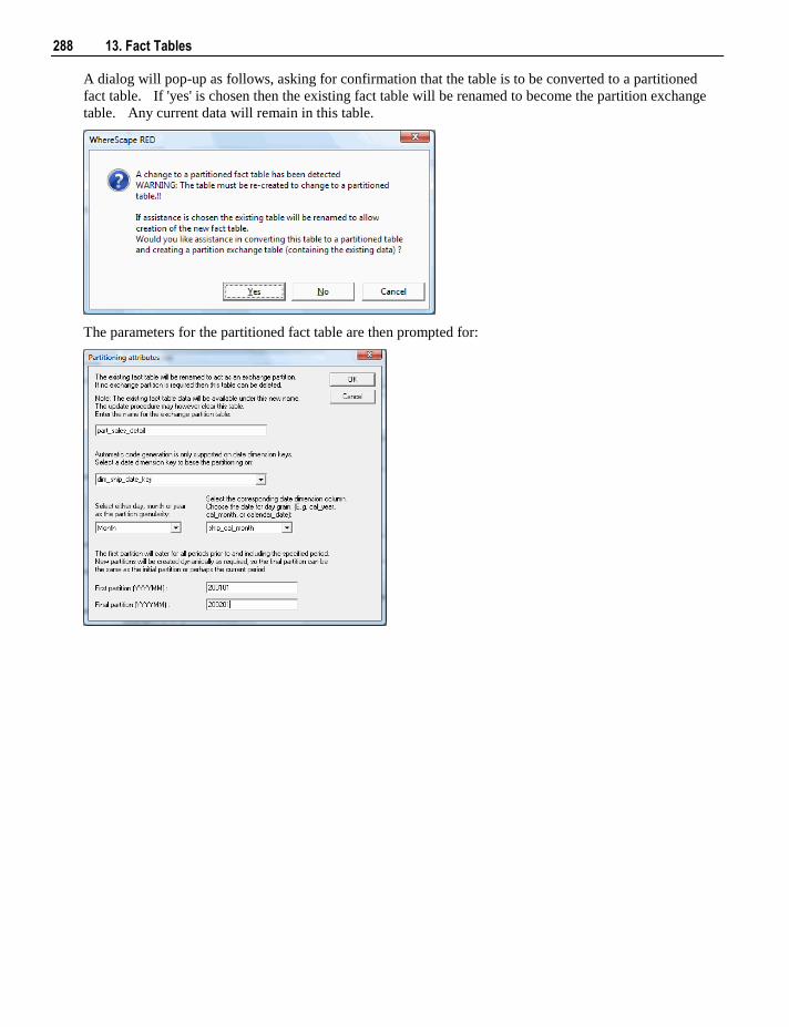
288 13. Fact Tables
A dialog will pop-up as follows, asking for confirmation that the table is to be converted to a partitioned
fact table. If 'yes' is chosen then the existing fact table will be renamed to become the partition exchange
table. Any current data will remain in this table.
The parameters for the partitioned fact table are then prompted for:
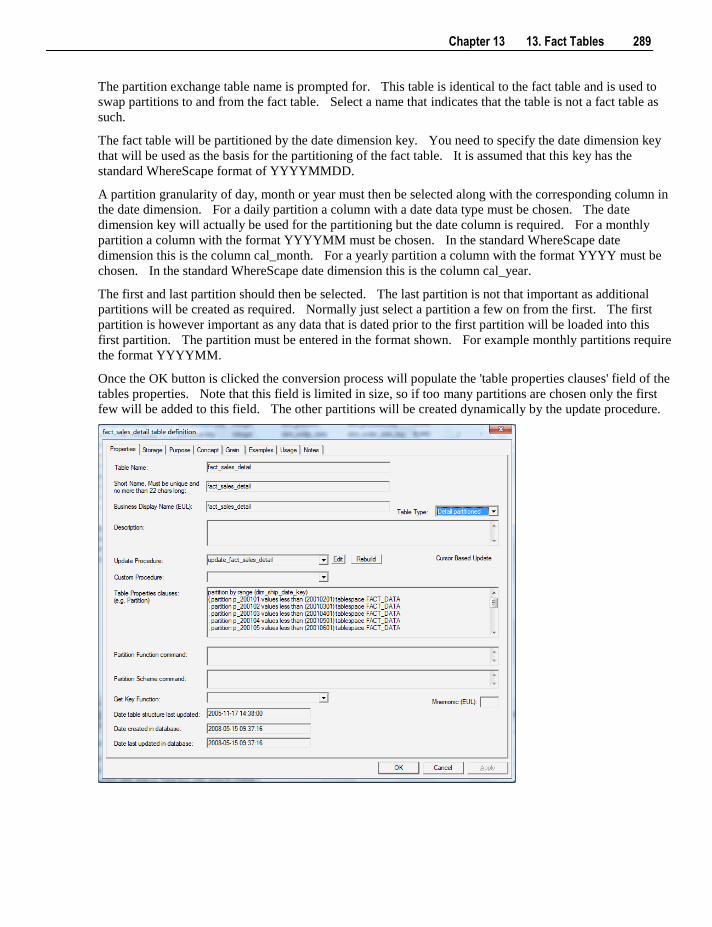
Chapter 13 13. Fact Tables 289
The partition exchange table name is prompted for. This table is identical to the fact table and is used to
swap partitions to and from the fact table. Select a name that indicates that the table is not a fact table as
such.
The fact table will be partitioned by the date dimension key. You need to specify the date dimension key
that will be used as the basis for the partitioning of the fact table. It is assumed that this key has the
standard WhereScape format of YYYYMMDD.
A partition granularity of day, month or year must then be selected along with the corresponding column in
the date dimension. For a daily partition a column with a date data type must be chosen. The date
dimension key will actually be used for the partitioning but the date column is required. For a monthly
partition a column with the format YYYYMM must be chosen. In the standard WhereScape date
dimension this is the column cal_month. For a yearly partition a column with the format YYYY must be
chosen. In the standard WhereScape date dimension this is the column cal_year.
The first and last partition should then be selected. The last partition is not that important as additional
partitions will be created as required. Normally just select a partition a few on from the first. The first
partition is however important as any data that is dated prior to the first partition will be loaded into this
first partition. The partition must be entered in the format shown. For example monthly partitions require
the format YYYYMM.
Once the OK button is clicked the conversion process will populate the 'table properties clauses' field of the
tables properties. Note that this field is limited in size, so if too many partitions are chosen only the first
few will be added to this field. The other partitions will be created dynamically by the update procedure.
290 13. Fact Tables
Click the OK button on the table properties dialog to begin the process of converting the fact table, creating
the new fact table and building the new update procedure. Examine the results screen to see what has been
done.
The partitioned fact table update procedure
The generated procedure will handle the creation of new partitions as required. Any data for periods prior
to the first partition is placed in the first partition. If data is received for a period after the last partition
then new partitions are created. Empty partitions are created if necessary to skip periods where no data is
present. For example, if we have a table partitioned by month and the latest partition is 200204
(april/2002). If data is then received for say september 2002 the update procedure will build partitions for
may, june, july, august and september. There is a variable at the start of the update procedure called
v_max_skip_periods. This variable is by default set to 12. This defines the maximum number of
continuous partitions we will leave empty. From our previous example if our latest partition was april
2002 and we received data for july 2003 with no interim data then the update procedure will fail as it would
have to skip 14 partitions. This check is present to prevent erroneous data from creating hundreds of
partitions into the future.
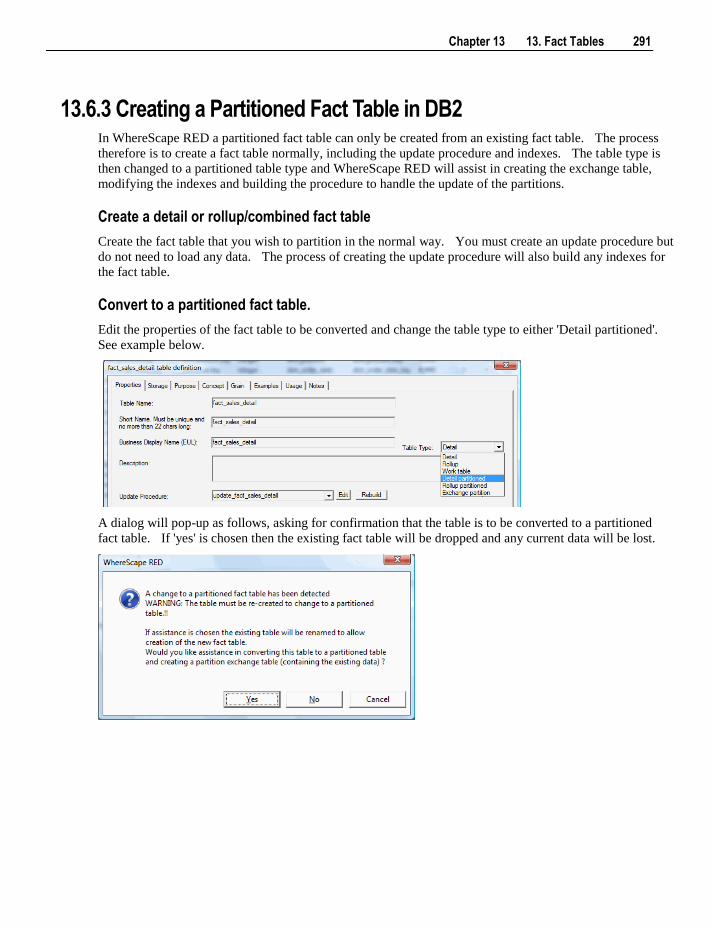
Chapter 13 13. Fact Tables 291
13.6.3 Creating a Partitioned Fact Table in DB2 In WhereScape RED a partitioned fact table can only be created from an existing fact table. The process
therefore is to create a fact table normally, including the update procedure and indexes. The table type is
then changed to a partitioned table type and WhereScape RED will assist in creating the exchange table,
modifying the indexes and building the procedure to handle the update of the partitions.
Create a detail or rollup/combined fact table
Create the fact table that you wish to partition in the normal way. You must create an update procedure but
do not need to load any data. The process of creating the update procedure will also build any indexes for
the fact table.
Convert to a partitioned fact table.
Edit the properties of the fact table to be converted and change the table type to either 'Detail partitioned'.
See example below.
A dialog will pop-up as follows, asking for confirmation that the table is to be converted to a partitioned
fact table. If 'yes' is chosen then the existing fact table will be dropped and any current data will be lost.
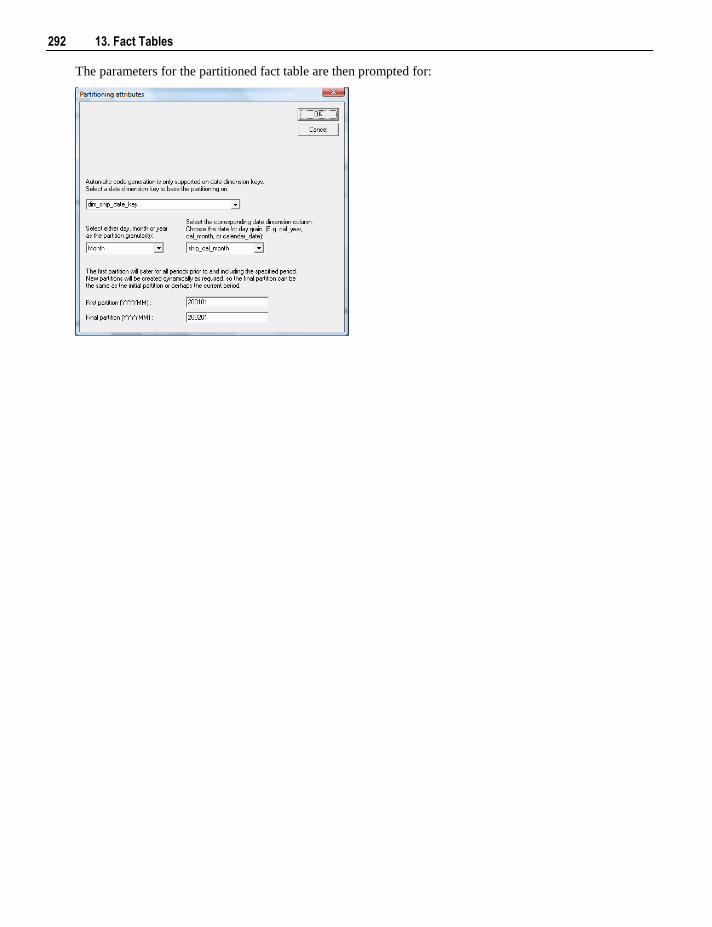
292 13. Fact Tables
The parameters for the partitioned fact table are then prompted for:
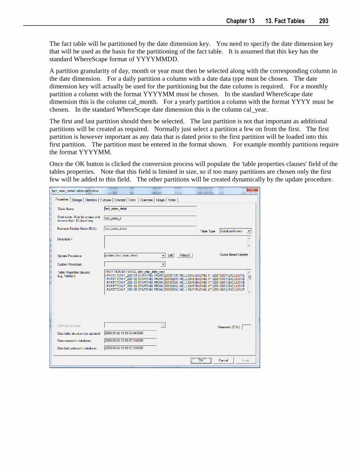
Chapter 13 13. Fact Tables 293
The fact table will be partitioned by the date dimension key. You need to specify the date dimension key
that will be used as the basis for the partitioning of the fact table. It is assumed that this key has the
standard WhereScape format of YYYYMMDD.
A partition granularity of day, month or year must then be selected along with the corresponding column in
the date dimension. For a daily partition a column with a date data type must be chosen. The date
dimension key will actually be used for the partitioning but the date column is required. For a monthly
partition a column with the format YYYYMM must be chosen. In the standard WhereScape date
dimension this is the column cal_month. For a yearly partition a column with the format YYYY must be
chosen. In the standard WhereScape date dimension this is the column cal_year.
The first and last partition should then be selected. The last partition is not that important as additional
partitions will be created as required. Normally just select a partition a few on from the first. The first
partition is however important as any data that is dated prior to the first partition will be loaded into this
first partition. The partition must be entered in the format shown. For example monthly partitions require
the format YYYYMM.
Once the OK button is clicked the conversion process will populate the 'table properties clauses' field of the
tables properties. Note that this field is limited in size, so if too many partitions are chosen only the first
few will be added to this field. The other partitions will be created dynamically by the update procedure.

294 13. Fact Tables
Click the OK button on the table properties dialog to begin the process of converting the fact table to be
partitioned. This drops and re-creates the fact table in DB2. The new update procedure is also generated
and compiled. Examine the results screen to see what has been done.
The partitioned fact table update procedure
The generated procedure will handle the creation of new partitions as required. Any data for periods prior
to the first partition is placed in the first partition. If data is received for a period after the last partition
then new partitions are created. Empty partitions are created if necessary to skip periods where no data is
present. For example, if we have a table partitioned by month and the latest partition is 200204
(april/2002). If data is then received for say september 2002 the update procedure will build partitions for
may, june, july, august and september. There is a variable at the start of the update procedure called
v_max_skip_periods. This variable is by default set to 12. This defines the maximum number of
continuous partitions we will leave empty. From our previous example if our latest partition was april
2002 and we received data for july 2003 with no interim data then the update procedure will fail as it would
have to skip 14 partitions. This check is present to prevent erroneous data from creating hundreds of
partitions into the future.
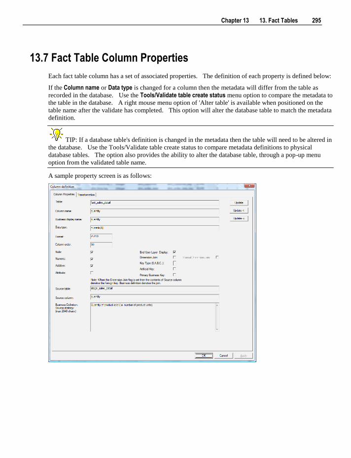
Chapter 13 13. Fact Tables 295
13.7 Fact Table Column Properties
Each fact table column has a set of associated properties. The definition of each property is defined below:
If the Column name or Data type is changed for a column then the metadata will differ from the table as
recorded in the database. Use the Tools/Validate table create status menu option to compare the metadata to
the table in the database. A right mouse menu option of 'Alter table' is available when positioned on the
table name after the validate has completed. This option will alter the database table to match the metadata
definition.
TIP: If a database table's definition is changed in the metadata then the table will need to be altered in
the database. Use the Tools/Validate table create status to compare metadata definitions to physical
database tables. The option also provides the ability to alter the database table, through a pop-up menu
option from the validated table name.
A sample property screen is as follows:
296 13. Fact Tables
The two special update keys allow you to update the column and step either forward or backward to the
next column's properties. ALT-Left Arrow and ALT-Right Arrow can also be used instead of the two special
update keys.
Table
The table to which the column belongs. Read only.
Column name
The database name of the column. This name must conform to database column naming standards.
Typically such standards exclude the use of spaces etc. A good practice is to only use alphanumerics and
the underscore character. Changing this field alters the table's definition.
Business display name
This defines how the business refers to this column. It does not affect the physical table definition, but
rather provides input to the documentation and to the view ws_admin_v_fact_col which can be used to assist
in the population of an end user tool's end user layer. As such it is a free form entry and any characters are
valid.
Data type
This is the database specific data type. It must be a valid data type for the data warehouse database
platform. Typical Oracle data types are number, char(), varchar2() and date. For SQL Server common
types are integer, numeric, varchar() and datetime. See the database documentation for a description of the
data types available. Changing this field alters the table's definition.
Format
This field is to allow the definition of a format mask for end user tools. It does not affect the physical table
definition, but rather provides input to the view ws_admin_v_fact_col which can be used to assist in the
population of an end user tool's end user layer. As such it is a free form entry and any characters are valid.
Typically format masks are only used on numeric fields. Example: #,###0.00. It is not worth the effort of
populating this field unless it can be utilized by the end user tools in use.
Column order
This numeric field provides the ordering of the columns in the database table create statement. The lowest
numbered column will appear first in the table. Although this affects the physical table definition no action
will be taken unless the table is re-created in the database. The columns can be re-numbered based on the
existing order by choosing the 'Respace order number' pop-up menu option when positioned over any
column in the table. This action will number the columns in increments of 10 starting at 10. In addition to
a simple change of the order field, the column order can be changed by first displaying the columns in the
middle pane and then using drag and drop to move the columns around. This drag and drop process will
automatically renumber the columns as required.
Nulls
This checkbox when set allows nulls to exist in this column. If cleared then nulls are not permitted in the
column.
Numeric
Chapter 13 13. Fact Tables 297
This checkbox indicates that the column in question is numeric when set. It does not affect the physical
table definition, but rather provides input to the view ws_admin_v_fact_col which can be used to assist in the
population of an end user tools end user layer. The use of this field is not relevant unless it can be utilized
by the end user tools.
Additive
This checkbox indicates that the column in question is additive when set. This implies that the column can
be summed when performing data grouping in a query. It does not affect the physical table definition, but
rather provides input to the view ws_admin_v_fact_col which can be used to assist in the population of an
end user tool's end user layer. The use of this field is not relevant unless it can be utilized by the end user
tools.
Attribute
This checkbox indicates that the column in question is an attribute when set. An attribute is defined as a
column that is non factual. For example we may have an order number, or a invoice number stored in the
fact table. Such columns are considered attributes, rather than facts. This checkbox does not affect the
physical table definition, but rather provides input to the view ws_admin_v_fact_col which can be used to
assist in the population of an end user tool's end user layer. The use of this field is not relevant unless it
can be utilized by the end user tools.
Source table
Indicates the table from which the column was sourced. This source table is normally a stage table within
the data warehouse. If the column was sourced from multiple stage tables, then the normal practice is to
record one of the tables in this field and a comment listing all of the other tables in the 'Business definition /
Source strategy' field. This field is used when generating a procedure to update the fact table. It is also
used in the track back diagrams and in the documentation.
If the column is a dimension join then the table shown will be the dimension table to which we are joining.
A dimension join will have the 'Dimension Join' checkbox set. Such joins are visible in the view
ws_admin_v_fact_join.
Source column
Indicates the column in the 'Source table' from which the column was sourced. Such a column is normally
a stage table column or a dimension table column.
If the column is a dimension join then the column shown will be the dimension table key column to which
we are joining. A dimension join will have the 'Dimension Join' checkbox set. Such joins are visible in
the view ws_admin_v_fact_join.
Business definition / Source strategy
Normally this field will contain a business definition of the column. Such a definition may be a description
of the column from a business user's point of view. This field might additionally contain information on
where and how the column was acquired. For example if the column is sourced from multiple tables or is a
composite or derived column then this definition would normally describe the process used to populate the
column. This field is used in the documentation and is available via the view ws_admin_v_fact_col . This
field is also stored as a comment against the column in the database.
Column Type
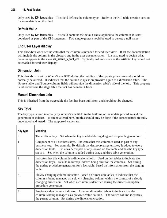
298 13. Fact Tables
Only used by KPI fact tables. This field defines the column type. Refer to the KPI table creation section
for more details on this field.
Default Value
Only used by KPI fact tables. This field contains the default value applied to the column if it is not
populated as part of the KPI statement. Two single quotes should be used to denote a null value.
End User Layer display
This checkbox when set indicates that the column is intended for end user view. If set the documentation
will include the column in the glossary and in the user documentation. It is also used to decide what
columns appear in the view ws_admin_v_fact_col. Typically columns such as the artificial key would not
be enabled for end user display.
Dimension Join
This checkbox is set by WhereScape RED during the building of the update procedure and should not
normally be altered. It indicates that the column in question provides a join to a dimension table. The
'Source table' and 'Source column' fields will provide the dimension table's side of the join. This property
is inherited from the stage table the fact has been built from.
Manual Dimension Join
This is inherited from the stage table the fact has been built from and should not be changed.
Key Type
The key type is used internally by WhereScape RED in the building of the update procedure and the
generation of indexes. It can be altered here, but this should only be done if the consequences are fully
understood and tested. The supported values are:
Key type Meaning
0 The artificial key. Set when the key is added during drag and drop table generation.
1 Component of all business keys. Indicates that this column is used as part of any
business key. For example: By default the dss_source_system_key is added to every
dimension table. It is considered part of any lookup on that table and has the key type
set to 1. Set when the column is added during drag and drop table generation.
2 Indicates that this column is a dimensional join. Used on fact tables to indicate the
dimension keys. Results in bitmap indexes being built for the columns. Set during
the update procedure generation for a fact table, based on information from the staging
table.
3 Slowly changing column indicator. Used on dimension tables to indicate that the
column is being managed as a slowly changing column within the context of a slowly
changing dimension. Set when a column is identified during the dimension update
procedure generation.
4 Previous value column indicator. Used on dimension tables to indicate that the
column is being managed as a previous value column. The source column identifies
the parent column. Set during the dimension creation.
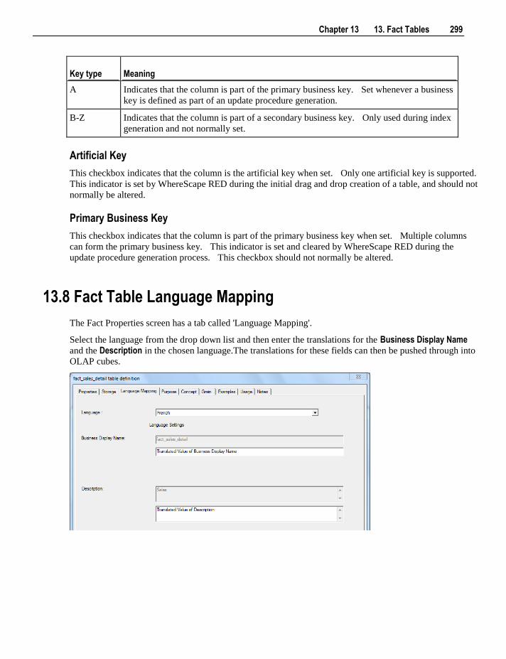
Chapter 13 13. Fact Tables 299
Key type Meaning
A Indicates that the column is part of the primary business key. Set whenever a business
key is defined as part of an update procedure generation.
B-Z Indicates that the column is part of a secondary business key. Only used during index
generation and not normally set.
Artificial Key
This checkbox indicates that the column is the artificial key when set. Only one artificial key is supported.
This indicator is set by WhereScape RED during the initial drag and drop creation of a table, and should not
normally be altered.
Primary Business Key
This checkbox indicates that the column is part of the primary business key when set. Multiple columns
can form the primary business key. This indicator is set and cleared by WhereScape RED during the
update procedure generation process. This checkbox should not normally be altered.
13.8 Fact Table Language Mapping
The Fact Properties screen has a tab called 'Language Mapping'.
Select the language from the drop down list and then enter the translations for the Business Display Name
and the Description in the chosen language.The translations for these fields can then be pushed through into
OLAP cubes.

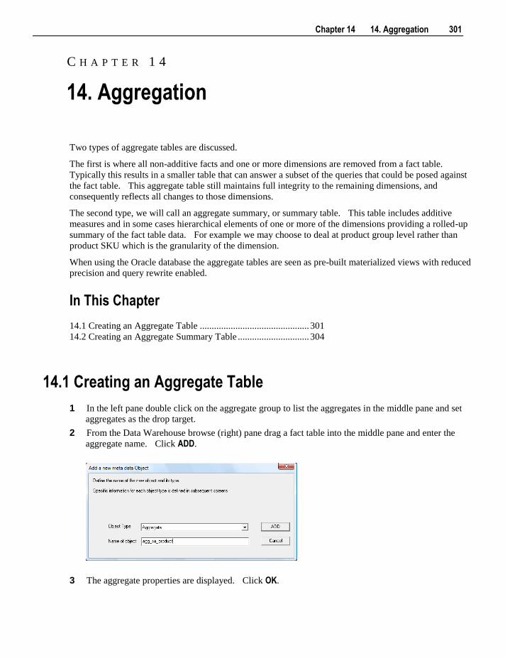
Chapter 14 14. Aggregation 301
Two types of aggregate tables are discussed.
The first is where all non-additive facts and one or more dimensions are removed from a fact table.
Typically this results in a smaller table that can answer a subset of the queries that could be posed against
the fact table. This aggregate table still maintains full integrity to the remaining dimensions, and
consequently reflects all changes to those dimensions.
The second type, we will call an aggregate summary, or summary table. This table includes additive
measures and in some cases hierarchical elements of one or more of the dimensions providing a rolled-up
summary of the fact table data. For example we may choose to deal at product group level rather than
product SKU which is the granularity of the dimension.
When using the Oracle database the aggregate tables are seen as pre-built materialized views with reduced
precision and query rewrite enabled.
In This Chapter
14.1 Creating an Aggregate Table .............................................. 301
14.2 Creating an Aggregate Summary Table .............................. 304
14.1 Creating an Aggregate Table
1 In the left pane double click on the aggregate group to list the aggregates in the middle pane and set
aggregates as the drop target.
2 From the Data Warehouse browse (right) pane drag a fact table into the middle pane and enter the
aggregate name. Click ADD.
3 The aggregate properties are displayed. Click OK.
C H A P T E R 1 4
14. Aggregation
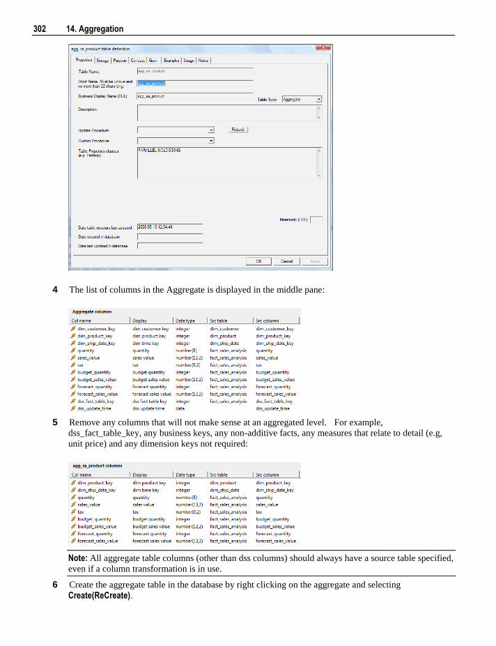
302 14. Aggregation
4 The list of columns in the Aggregate is displayed in the middle pane:
5 Remove any columns that will not make sense at an aggregated level. For example,
dss_fact_table_key, any business keys, any non-additive facts, any measures that relate to detail (e.g,
unit price) and any dimension keys not required:
Note: All aggregate table columns (other than dss columns) should always have a source table specified,
even if a column transformation is in use.
6 Create the aggregate table in the database by right clicking on the aggregate and selecting
Create(ReCreate).
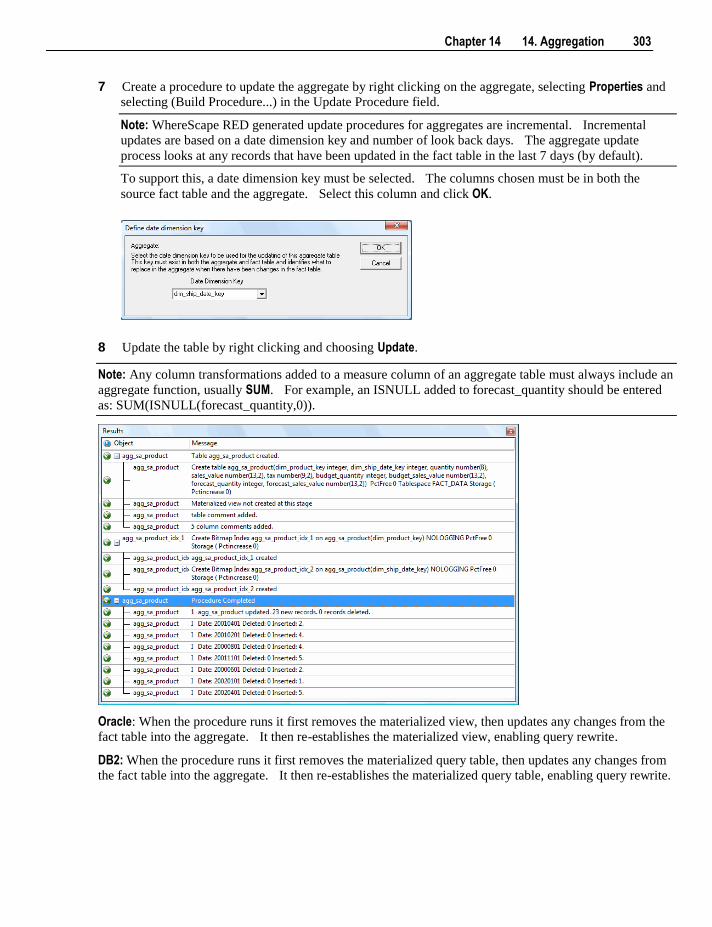
Chapter 14 14. Aggregation 303
7 Create a procedure to update the aggregate by right clicking on the aggregate, selecting Properties and
selecting (Build Procedure...) in the Update Procedure field.
Note: WhereScape RED generated update procedures for aggregates are incremental. Incremental
updates are based on a date dimension key and number of look back days. The aggregate update
process looks at any records that have been updated in the fact table in the last 7 days (by default).
To support this, a date dimension key must be selected. The columns chosen must be in both the
source fact table and the aggregate. Select this column and click OK.
8 Update the table by right clicking and choosing Update.
Note: Any column transformations added to a measure column of an aggregate table must always include an
aggregate function, usually SUM. For example, an ISNULL added to forecast_quantity should be entered
as: SUM(ISNULL(forecast_quantity,0)).
Oracle: When the procedure runs it first removes the materialized view, then updates any changes from the
fact table into the aggregate. It then re-establishes the materialized view, enabling query rewrite.
DB2: When the procedure runs it first removes the materialized query table, then updates any changes from
the fact table into the aggregate. It then re-establishes the materialized query table, enabling query rewrite.
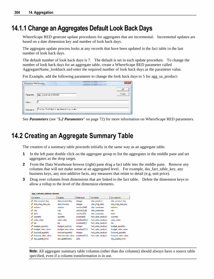
304 14. Aggregation
14.1.1 Change an Aggregates Default Look Back Days WhereScape RED generate update procedures for aggregates that are incremental. Incremental updates are
based on a date dimension key and number of look back days.
The aggregate update process looks at any records that have been updated in the fact table in the last
number of look back days.
The default number of look back days is 7. The default is set in each update procedure. To change the
number of look back days for an aggregate table, create a WhereScape RED parameter called
AggregateName_lookback and enter the required number of look back days as the parameter value.
For Example, add the following parameter to change the look back days to 5 for agg_sa_product:
See Parameters (see "5.2 Parameters" on page 72) for more information on WhereScape RED parameters.
14.2 Creating an Aggregate Summary Table
The creation of a summary table proceeds initially in the same way as an aggregate table.
1 In the left pane double click on the aggregate group to list the aggregates in the middle pane and set
aggregates as the drop target.
2 From the Data Warehouse browse (right) pane drag a fact table into the middle pane. Remove any
columns that will not make sense at an aggregated level. For example, dss_fact_table_key, any
business keys, any non-additive facts, any measures that relate to detail (e.g, unit price).
3 Drag over columns from dimensions that are linked to the fact table. Delete the dimension keys to
allow a rollup to the level of the dimension elements.
Note: All aggregate summary table columns (other than dss columns) should always have a source table
specified, even if a column transformation is in use.
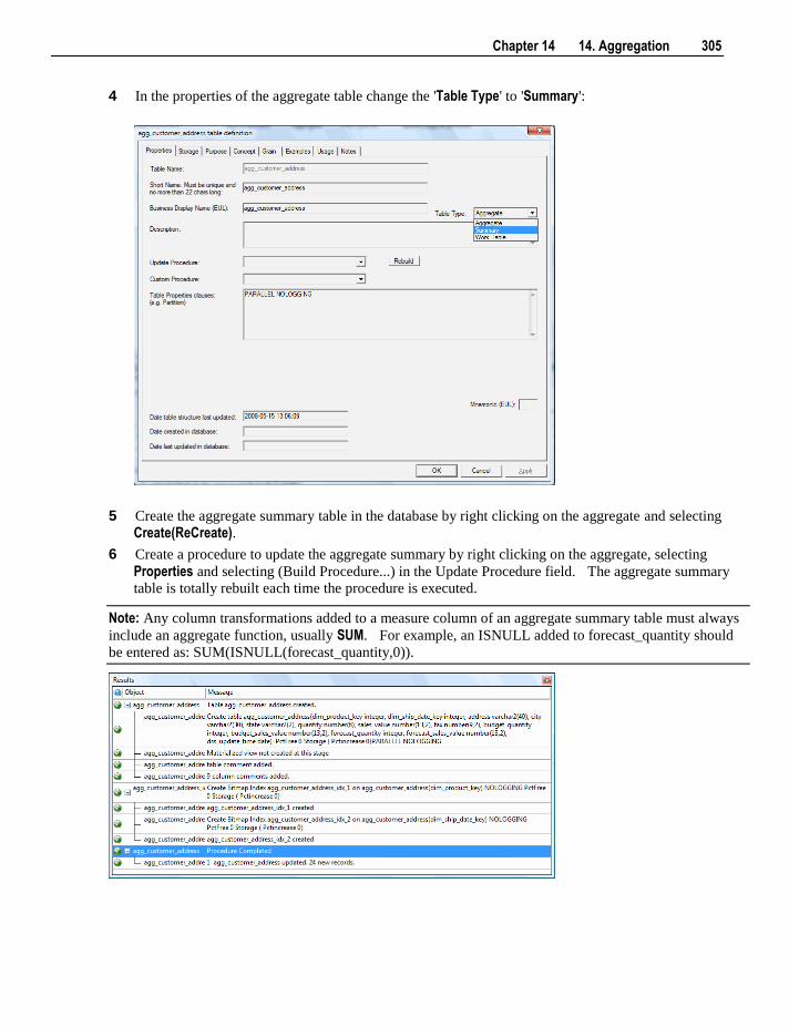
Chapter 14 14. Aggregation 305
4 In the properties of the aggregate table change the 'Table Type' to 'Summary':
5 Create the aggregate summary table in the database by right clicking on the aggregate and selecting
Create(ReCreate).
6 Create a procedure to update the aggregate summary by right clicking on the aggregate, selecting
Properties and selecting (Build Procedure...) in the Update Procedure field. The aggregate summary
table is totally rebuilt each time the procedure is executed.
Note: Any column transformations added to a measure column of an aggregate summary table must always
include an aggregate function, usually SUM. For example, an ISNULL added to forecast_quantity should
be entered as: SUM(ISNULL(forecast_quantity,0)).

Chapter 15 15. Views 307
Views are normally created from dimensions. These views are then used to define dimensions in a fact
table where the dimension appears multiple times. A classic example is that of the date dimension. In our
tutorials we create a fact table that has two date dimensions. An order date and a ship date dimension. To
facilitate the creation of the fact table we create two dimension views to allow the date dimension to be
joined to the fact table twice.
Views can also be created from any other table type. By default views are visualized as part of the
dimension object group. If fact table views or other views are being used then views can be visualized as a
separate object type by checking the appropriate box under the Tools/Options menu item.
In This Chapter
15.1 Creating a Dimension View ................................................ 308
15.2 Non-Dimension Object Views ............................................ 313
15.3 Creating a Custom View ..................................................... 316
15.4 Dimension View Language Mapping ................................. 318
C H A P T E R 1 5
15. Views
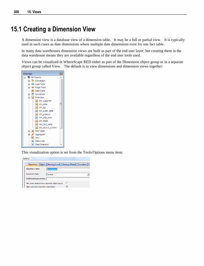
308 15. Views
15.1 Creating a Dimension View
A dimension view is a database view of a dimension table. It may be a full or partial view. It is typically
used in such cases as date dimensions where multiple date dimensions exist for one fact table.
In many data warehouses dimension views are built as part of the end user layer, but creating them in the
data warehouse means they are available regardless of the end user tools used.
Views can be visualized in WhereScape RED either as part of the Dimension object group or in a separate
object group called View. The default is to view dimensions and dimension views together:
This visualization option is set from the Tools/Options menu item:
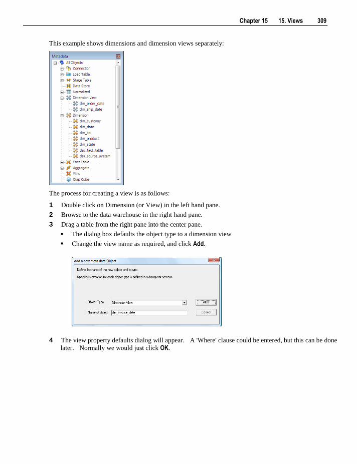
Chapter 15 15. Views 309
This example shows dimensions and dimension views separately:
The process for creating a view is as follows:
1 Double click on Dimension (or View) in the left hand pane.
2 Browse to the data warehouse in the right hand pane.
3 Drag a table from the right pane into the center pane.
The dialog box defaults the object type to a dimension view
Change the view name as required, and click Add.
4 The view property defaults dialog will appear. A 'Where' clause could be entered, but this can be done
later. Normally we would just click OK.
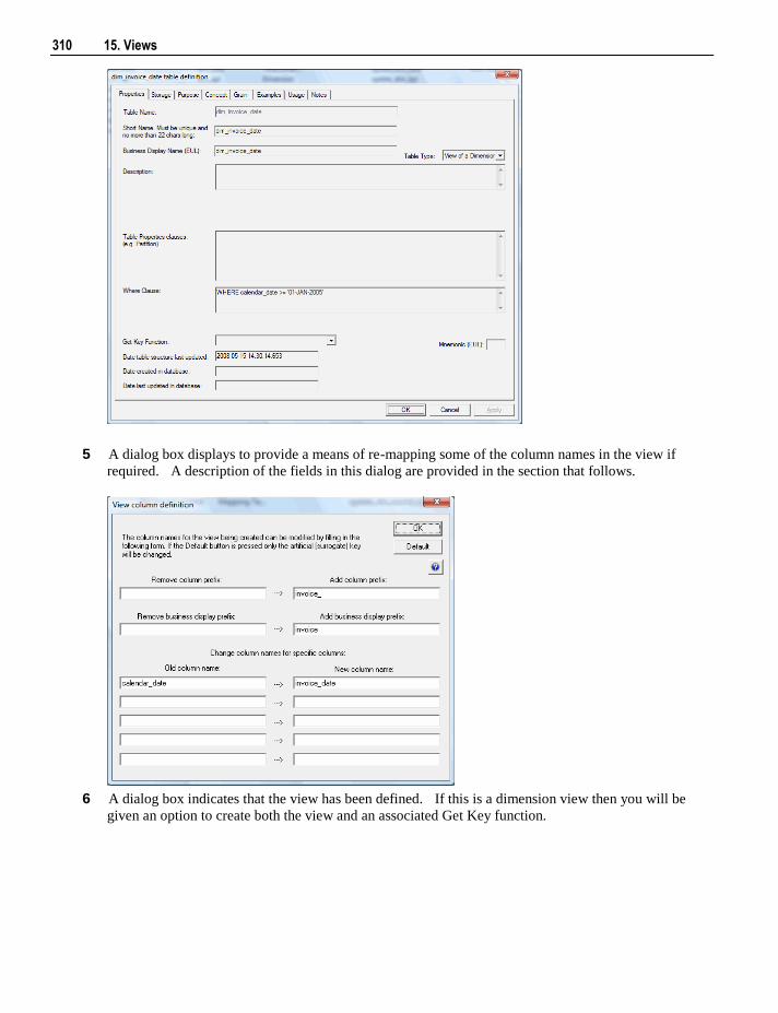
310 15. Views
5 A dialog box displays to provide a means of re-mapping some of the column names in the view if
required. A description of the fields in this dialog are provided in the section that follows.
6 A dialog box indicates that the view has been defined. If this is a dimension view then you will be
given an option to create both the view and an associated Get Key function.
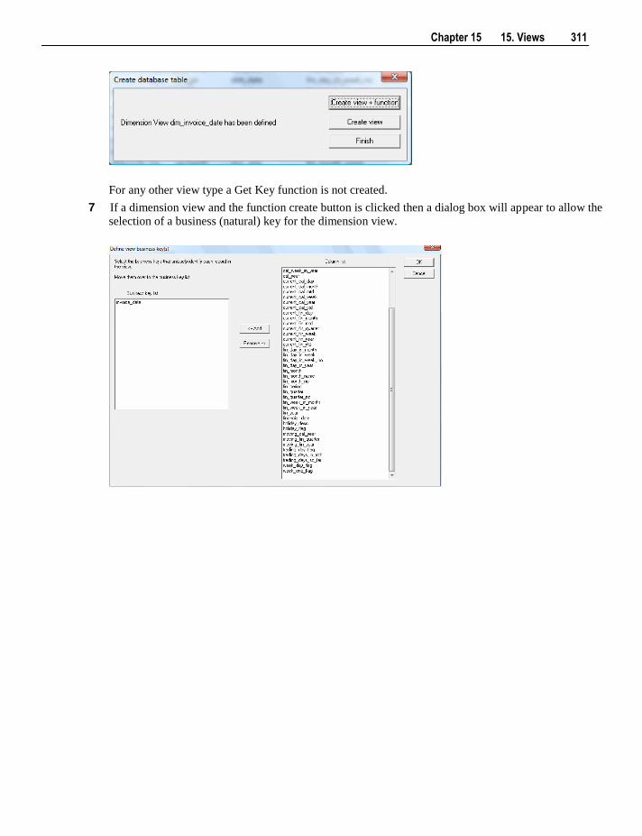
Chapter 15 15. Views 311
For any other view type a Get Key function is not created.
7 If a dimension view and the function create button is clicked then a dialog box will appear to allow the
selection of a business (natural) key for the dimension view.
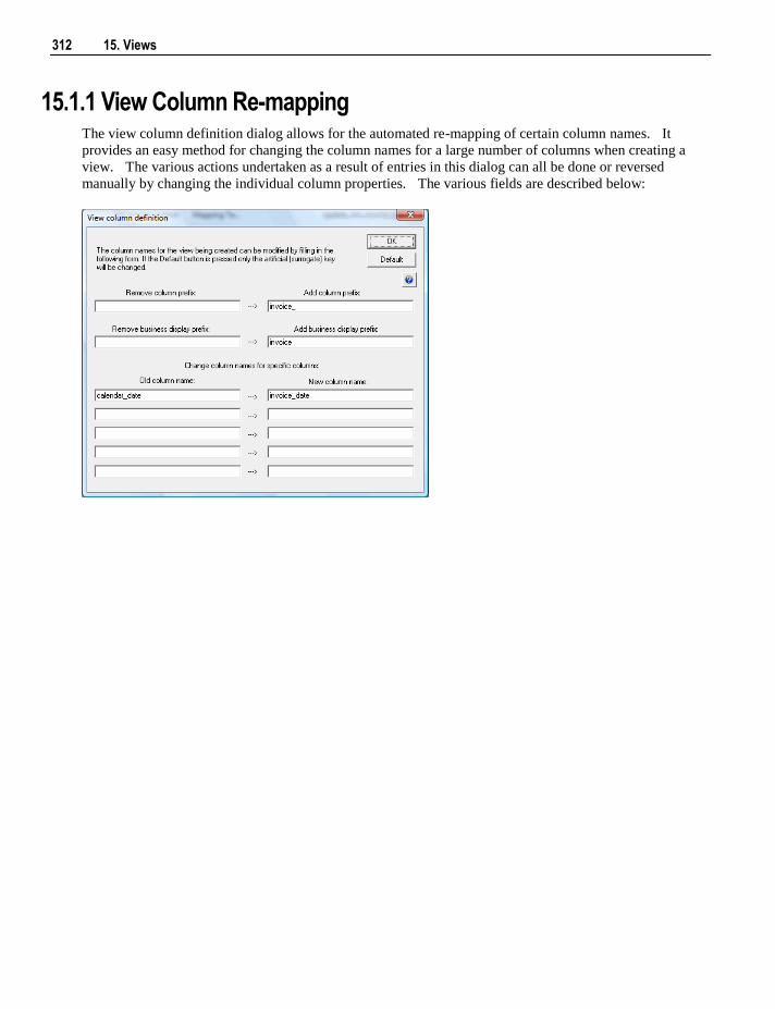
312 15. Views
15.1.1 View Column Re-mapping The view column definition dialog allows for the automated re-mapping of certain column names. It
provides an easy method for changing the column names for a large number of columns when creating a
view. The various actions undertaken as a result of entries in this dialog can all be done or reversed
manually by changing the individual column properties. The various fields are described below:
Chapter 15 15. Views 313
Remove column prefix
If the columns in the source table are prefixed then that prefix can be removed by entering it in this field.
An example may be a date dimension which has each column prefixed with date_ (e.g. date_month,
date_year etc.). If this field is left blank then no removal action is taken.
Add column prefix
If required a prefix can be added to each column name. This is particularly useful when defining a date
dimension view where you would like each column to be prefixed by the date type.
Remove business display prefix
As per the column names it may be required to remove a prefix from the business display fields. If so enter
the prefix to remove in this column.
Add business display prefix
The business display fields are used in the creation of the glossary. It is therefore quite useful to prefix
these display fields with an identifier for the view being created. It is assumed that these business display
names will be carried forward to the end user layer. Enter a value in this field to prefix the business
display name fields for each column. It is normal to include a space at the end of this field.
Old column name
Up to five individual column names can be re mapped. Enter the column name as it appears in the source
table in one of the 'old column name' fields in order to re map that column name. The business display
name is also changed to match.
New column name
Place a new column name alongside any existing column name you wish to re map. In the example dialog
above a column named 'calendar_date' is being renamed to 'order_date' in the view.
15.2 Non-Dimension Object Views
WhereScape RED also supports creating views of objects other that dimensions (load tables, facts, stage
tables, aggregates, ...).
A fact view is a database view of a fact table. It may be a full, partial view, or a view incorporating both
the fact data and some dimensional attributes. It is typically used in cases where a subset of information is
to be provided for specific end user communities. It is common that the 'Where' clause be populated in fact
views, either to join the dimension tables or restrict the data that the view represents.
Similarly, views may be created over staging tables or any other table object.
The creation of non-dimension table views is the same process as that for dimension views:
1 Drag a table from the right pane into the center pane.
2 The dialog box defaults the object type to a view.
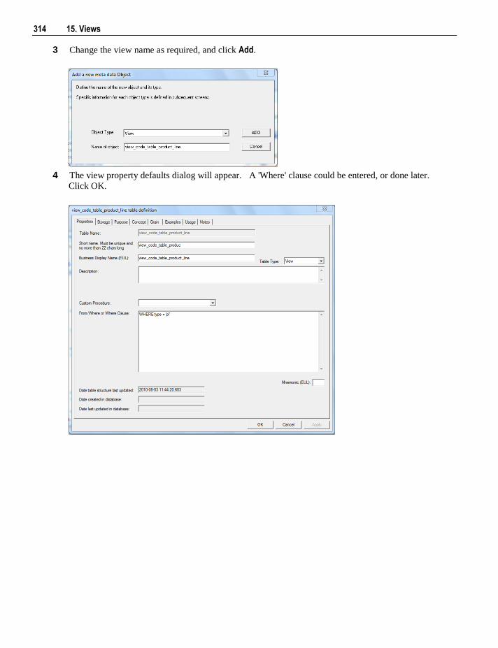
314 15. Views
3 Change the view name as required, and click Add.
4 The view property defaults dialog will appear. A 'Where' clause could be entered, or done later.
Click OK.
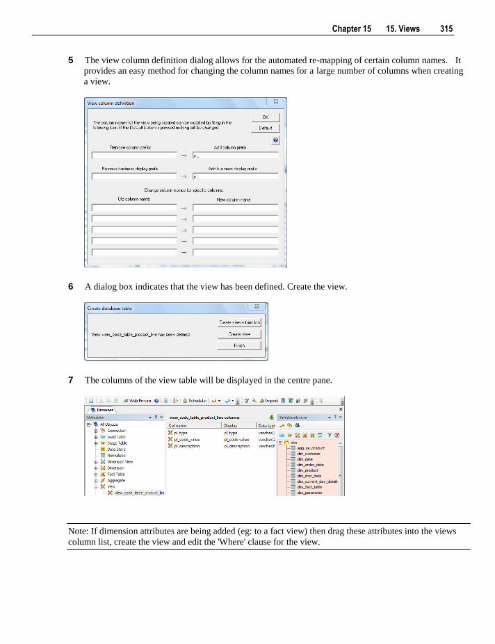
Chapter 15 15. Views 315
5 The view column definition dialog allows for the automated re-mapping of certain column names. It
provides an easy method for changing the column names for a large number of columns when creating
a view.
6 A dialog box indicates that the view has been defined. Create the view.
7 The columns of the view table will be displayed in the centre pane.
Note: If dimension attributes are being added (eg: to a fact view) then drag these attributes into the views
column list, create the view and edit the 'Where' clause for the view.
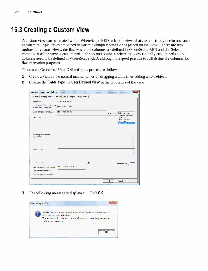
316 15. Views
15.3 Creating a Custom View
A custom view can be created within WhereScape RED to handle views that are not strictly one to one such
as where multiple tables are joined or where a complex condition is placed on the view. There are two
options for custom views, the first where the columns are defined in WhereScape RED and the 'Select'
component of the view is customized. The second option is where the view is totally customized and no
columns need to be defined in WhereScape RED, although it is good practice to still define the columns for
documentation purposes.
To create a Custom or 'User Defined' view proceed as follows:
1 Create a view in the normal manner either by dragging a table in or adding a new object.
2 Change the 'Table Type' to 'User Defined View' in the properties of the view.
3 The following message is displayed. Click OK.
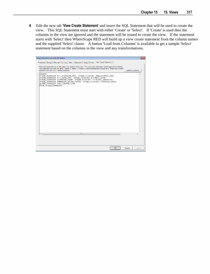
Chapter 15 15. Views 317
4 Edit the new tab 'View Create Statement' and insert the SQL Statement that will be used to create the
view. This SQL Statement must start with either 'Create' or 'Select'. If 'Create' is used then the
columns in the view are ignored and the statement will be issued to create the view. If the statement
starts with 'Select' then WhereScape RED will build up a view create statement from the column names
and the supplied 'Select' clause. A button 'Load from Columns' is available to get a sample 'Select'
statement based on the columns in the view and any transformations.
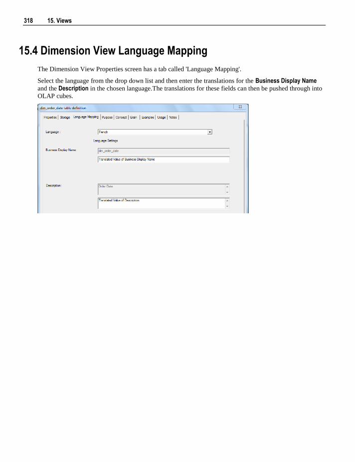
318 15. Views
15.4 Dimension View Language Mapping
The Dimension View Properties screen has a tab called 'Language Mapping'.
Select the language from the drop down list and then enter the translations for the Business Display Name
and the Description in the chosen language.The translations for these fields can then be pushed through into
OLAP cubes.
Chapter 16 16. Analysis Services OLAP Cubes 319
In This Chapter
16.1 Overview ............................................................................. 319
16.2 Defining an OLAP Cube ..................................................... 320
16.3 Inspecting and Modifying Advanced Cube Properties ........ 323
16.4 Creating an OLAP Cube on the Analysis Services Server .. 325
16.5 Cube Objects ....................................................................... 326
16.6 Dimension Objects .............................................................. 356
16.7 Changing OLAP Cubes ....................................................... 368
16.8 Retrofitting an OLAP Object .............................................. 370
16.1 Overview
A cube is a set of related measures and dimensions that is used to analyze data.
A measure is a transactional value or measurement that a user may want to aggregate. The source of
measures are usually columns in one or more source tables. Measures are grouped into measure groups.
A dimension is a group of attributes that represent an area of interest related to the measures in the cube
and which are used to analyze the measures in the cube. For example, a customer dimension might
include the attributes:
Customer Name
Customer Gender
Customer City
These would enable measures in the cube to be analyzed by Customer Name, Customer Gender, and
Customer City. The source of attributes are usually columns in one or more source tables. The
attributes within each dimension can be organized into hierarchies to provide paths for analysis.
C H A P T E R 1 6
16. Analysis Services OLAP Cubes
320 16. Analysis Services OLAP Cubes
A cube is then augmented with calculations, key performance indicators (generally known as KPIs), actions,
partitions, perspectives, and translations.
The information required to build and support an Analysis Services cube and its surrounding structure is
reasonably complex and diverse. In attempting to automate the building of Analysis Services cubes
WhereScape RED has simplified and restricted many of the functions available to the cube designer.
WhereScape RED includes most of the commonly used capabilities and the components that logically fit
into the methodology incorporated within WhereScape RED.
WhereScape RED broadly provides functionality to manage all of the above, except for perspectives and
translations. These can be created outside of WhereScape RED, scripted in xmla and executed from within
WhereScape RED. Features of cubes that are not supported in WhereScape RED can be added to the cube
via the Microsoft tools. These altered cubes can still be processed through the WhereScape RED
scheduler, and the cube should be documented within WhereScape RED to explain the post creation phases
required.
As a general rule, once a cube or a component of a cube is created on the Analysis Services server it cannot
be altered through WhereScape RED. The OLAP object can be dropped and recreated easily using RED.
New OLAP objects defined in RED (e.g. additional calculations or measures) can be added by recreating
the cube.
WhereScape RED supports cubes in Microsoft Sql Server Analysis Services versions 2005 and 2008.
16.2 Defining an OLAP Cube
OLAP Cubes can be created from fact, fact view or aggregate objects . A single cube can contain dates
from multiple source star schemas, each defined with a measure group. An OLAP Cube consists of many
parts namely, measure groups, measures, calculations, actions, dimensions, dimension hierarchies,
dimension attributes and dimension attribute relationships. It is strongly recommended that drag and drop
is used to create an OLAP Cube in order that all the components are set up correctly. OLAP Cubes can
utilize a hierarchical structure in the dimensions to facilitate user queries. Therefore each dimension
present in an OLAP Cube should have either a hierarchy of levels or attributes and relationships.. The
hierarchies are defined against the underlying dimensional attributes which can be inherited from the source
dimension metadata. Individual attributes can be added to the dimension after the OLAP Cube or OLAP
Dimension metadata has been created.
Building a New OLAP Cube
To create an OLAP Cube proceed as follows:
1 Double click on the 'OLAP Cube' object group to make the middle pane a cube drop target.
2 Select the data warehouse connection to browse in the source pane. The connection can be selected by
right clicking the Data Warehouse connection in the Object pane and choosing Browse Source System.
3 Drag a fact table from the source pane into the target pane.
4 Set the cube name in the 'Create new metadata Object' dialog box and click Add.
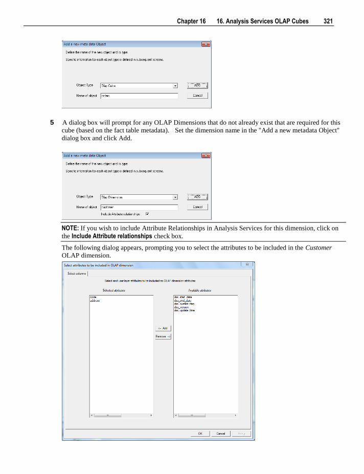
Chapter 16 16. Analysis Services OLAP Cubes 321
5 A dialog box will prompt for any OLAP Dimensions that do not already exist that are required for this
cube (based on the fact table metadata). Set the dimension name in the "Add a new metadata Object"
dialog box and click Add.
NOTE: If you wish to include Attribute Relationships in Analysis Services for this dimension, click on
the Include Attribute relationships check box.
The following dialog appears, prompting you to select the attributes to be included in the Customer
OLAP dimension.
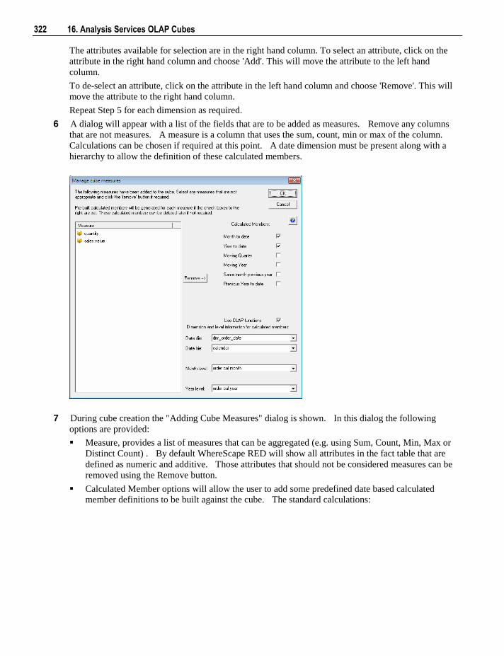
322 16. Analysis Services OLAP Cubes
The attributes available for selection are in the right hand column. To select an attribute, click on the
attribute in the right hand column and choose 'Add'. This will move the attribute to the left hand
column.
To de-select an attribute, click on the attribute in the left hand column and choose 'Remove'. This will
move the attribute to the right hand column.
Repeat Step 5 for each dimension as required.
6 A dialog will appear with a list of the fields that are to be added as measures. Remove any columns
that are not measures. A measure is a column that uses the sum, count, min or max of the column.
Calculations can be chosen if required at this point. A date dimension must be present along with a
hierarchy to allow the definition of these calculated members.
7 During cube creation the "Adding Cube Measures" dialog is shown. In this dialog the following
options are provided:
Measure, provides a list of measures that can be aggregated (e.g. using Sum, Count, Min, Max or
Distinct Count) . By default WhereScape RED will show all attributes in the fact table that are
defined as numeric and additive. Those attributes that should not be considered measures can be
removed using the Remove button.
Calculated Member options will allow the user to add some predefined date based calculated
member definitions to be built against the cube. The standard calculations:
Chapter 16 16. Analysis Services OLAP Cubes 323
Month to date
Year to date
Moving Quarter
Moving Year
Same Month Previous Year
Previous Year to date
These will define a calculated measure based on the associated drop down boxes. There are 2
different ways that WhereScape RED will implement these calculations which is dictated by the
Use OLAP functions check box:
Using OLAP Functions - will implement the calculations using MDX Expressions within the
cube using date based MDX functions. These calculations are efficiently executed by
Analysis Services.
Without using OLAP functions - will implement the calculations using an MDX Filter function
built over date dimension attributes. This option leverages the flags from the relational date
dimension and ensures that a query using the calculations in the Cube will match an equivalent
query against the star schema and is particularly useful if non-standard date periods are used.
8 The cube and dimensions will be created in WhereScape RED metadata and the cube measures will be
displayed.
Setting Cube Properties
The properties of the cube must be completed before we can create the cube in the Analysis services
database. Most of the elements in the properties screen will be defaulted, but each of the following
columns will probably need to be completed.
1 The connection to the Analysis services server must be defined within the cube properties. This
connection is a connection object. If no such connection exists then a new connection of type must be
created and configured. SQL Server 2005 or 2008 Analysis Services use a connection type of
"Analysis Server 2005+". This connection name must then be chosen in the cubes properties.
2 A cube database name must be selected. A new database name can be created by clicking the 'new
database' button. This database name is the database that the cubes will reside in on the Analysis
services server.
3 The data source connection must be defined and the three derived values shown under this connection
must be present. If there is nothing in the three fields below the data source connection then the
connection object will need to be modified. The provider type will normally be MSDAORA if the
data warehouse is an Oracle database or SQLOLEDB if the data warehouse is SQL Server. The Server
is either the SQL Server database server, or the Oracle TNS name. The database is the data warehouse
database name.
16.3 Inspecting and Modifying Advanced Cube Properties
Now that the basic OLAP Cube has been defined, various properties of the OLAP Cube can be inspected or
modified:
Measure Groups
1 Display the Measure Groups by selecting the right mouse menu option "Display Measure Groups"
when positioned on the cube name.
324 16. Analysis Services OLAP Cubes
2 Measure Group properties can be changed by using the right mouse menu option "Properties" when
positioned over the measure.
Measures
1 Display all of the Measures associated with a cube by selecting the right mouse menu option "Display
Measures" when positioned on the cube name.
2 The measure properties can be changed by using the right mouse menu option "Properties" when
positioned on a measure name.
Calculations
1 Display all of the Calculated members defined on the cube by selecting the right mouse menu option
"Display Calculations" when positioned on the cube name.
2 Calculated members can be changed by using the right mouse menu item "Properties" when positioned
on the calculation name.
KPIs
1 Display all of the KPIs defined on the cube by selecting the right mouse menu option "Display KPIs"
when positioned on the cube name.
2 KPIs can be changed by using the right mouse menu item "Properties" when positioned on the KPI
name.
Actions
1 Display all of the Actions defined on the cube by selecting the right mouse menu option "Display
Actions" when positioned on the cube name.
2 Actions can be changed by using the right mouse menu item "Properties" when positioned on the
Action name.
Partitions
1 Display all of the Partitions defined on the Measure Groups that are associated with the cube by
selecting the right mouse menu option "Display Partitions" when positioned on the cube name.
2 Partitions can be changed by using the right mouse menu item "Properties" when positioned on the
Partition name.
Dimensions
1 Display all of the OLAP Dimensions associated with the cube by selecting the right mouse menu
option 'Display Dimensions' when positioned on the cube name.
2 OLAP Dimension properties that are customisable for a cube can be changed by using the right mouse
menu item "Properties" when positioned on the OLAP Dimension name.
Measure Group Dimensions
1 Display the relationship of OLAP Dimensions to Measure Groups defined against the cube by selecting
the right mouse menu option 'Display Measure Group Dimensions' when positioned on the cube name.
2 The properties of the relationship of the OLAP Dimension to Measure Group that are customisable can
be changed by using the right mouse menu item "Properties" when positioned on the OLAP Dimension
name.
Chapter 16 16. Analysis Services OLAP Cubes 325
16.4 Creating an OLAP Cube on the Analysis Services Server
If all of the tasks above are completed then it should be possible to now create the cube on the Analysis
Services server. When positioned on the OLAP Cube name use the right mouse menu and select the Create Cube option. WhereScape RED will check that key components of the cube are correct before it proceeds
to issue the create command.
The create cube menu option will perform the following tasks on the Analysis Services server:
Create an Analysis Services database if the name specified is not already present.
Create a Data Source with connection information back to the data warehouse based on the cube source
information in the Data Warehouse connection.
Create a Data Source View to support the cube objects defined
Create the dimensions used by the cube as database shared dimensions if they do not already exist.
Create the cube if it does not exist
Create a partition for the cube.
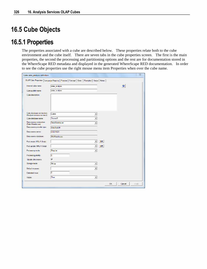
326 16. Analysis Services OLAP Cubes
16.5 Cube Objects
16.5.1 Properties The properties associated with a cube are described below. These properties relate both to the cube
environment and the cube itself. There are seven tabs in the cube properties screen. The first is the main
properties, the second the processing and partitioning options and the rest are for documentation stored in
the WhereScape RED metadata and displayed in the generated WhereScape RED documentation. In order
to see the cube properties use the right mouse menu item Properties when over the cube name.
Chapter 16 16. Analysis Services OLAP Cubes 327
Internal Cube Name
This is the name by which the cube is known within WhereScape RED. This name is limited to 64
characters in length and may contain only alphanumeric characters and underscores.
Cube Publish Name
This is the name that the cube will have in the Analysis Services server. It is not constrained in its content
except for the limitations imposed on it by Analysis Services.
Cube Description
A description of the cube. This is used both in the WhereScape RED documentation and is also stored
against the cube in Analysis Services.
Cube Database Connection
This field allows the selection of one of the existing connections defined within WhereScape RED. The
connection must be of type 'Microsoft Analysis Server 2005+'. If no such connection exists then a new
connection object must be created. This connection object is used to point to the Analysis Services server.
Cube Database Name
An Analysis Services server must have databases associated with it. Each database can contain one or
more cubes, dimensions, data sources etc. Select the name of an existing database on the server from the
drop down list. To create a new Database name, select '(Define New Cube Database)' from the drop down
list and the dialog that follows will allow you to register the name within the WhereScape RED metadata.
Once registered, the name can then be selected as the database.
Data Source Connection
In Analysis Services the data source is the location of the data to be used to build the cube. It also defines
the path for any drill through operations. This field provides a drop down of the existing connections.
The Data Warehouse connection must be chosen.
Data Source Provider Type
This field essentially defines what type of database the Data Warehouse is. The three options are
MSDAORA where the data source is an Oracle database. OLESQLDB where the data source is a SQL
Server database, or MSDASQL to define an ODBC source. The MSDASQL provider type could be used
for either Oracle or SQL Server data warehouses, but performance may be compromised. This field is a
read only field in the properties screen. Its value is set in the properties of the data source connection.
Data Source Server
The data source server is also a read only field being sourced from the properties of the data source
connection. For SQL Server it defines the server on which the data warehouse database runs. For Oracle
it is the TNS names entry for the database.
Data Source Database
328 16. Analysis Services OLAP Cubes
The data source database is also a read only field being sourced from the properties of the data source
connection. For SQL Server it defines the database in which the data warehouse runs. For Oracle it is
also the database name.
Post Create XML/A Script
This is an XML/A script that is run on the cube database when the cube is created. This script allows
Analysis Services features to be added to the cube or cube database that have been built outside of
WhereScape RED - for example security roles that has been defined for the cube can be recreated from the
script when the cube is created (or recreated).
Post Update XML/A Script
This is an XML/A script that is run on the cube database when the cube is updated or processed via the
scheduler. This script allows Analysis Services features to be added to the cube or cube database that have
been built outside of WhereScape RED - for example security roles that has been defined for the cube can
be recreated from the script when the cube is updated or processed.
Processing Mode
Gets or sets the index and aggregation settings for cube processing. The value indicates whether processed
data is available after all required data aggregation has been completed (Regular) or immediately after the
data has been loaded (Lazy Aggregations). This setting will be used as the default for new measure groups
and partitions created for the cube.
Processing Priority
Gets or sets the processing priority for the cube.
Update Dimensions
Will determine whether to process the OLAP Dimension related to the cube as part of the processing of the
cube.
Storage Mode
This field allows two options; MOLAP - Multidimensional OLAP or ROLAP.- Relational OLAP. At the
cube properties level, setting this field will determine the defaults for the Storage Mode field on its related
Measure Groups and partitions.
Default Measure
Specifies the measure used to resolve MDX expressions if a measure is not explicitly referenced in the
expression. If no default measure is specified an arbitrary measure is used as the default measure.
Estimated Rows
Specifies the estimated number of rows in the fact tables. Enter the size of the fact or source table if
known, otherwise leave as zero.
Visible
Indicates whether the cube is visible to client applications.
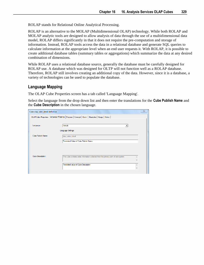
Chapter 16 16. Analysis Services OLAP Cubes 329
ROLAP stands for Relational Online Analytical Processing.
ROLAP is an alternative to the MOLAP (Multidimensional OLAP) technology. While both ROLAP and
MOLAP analytic tools are designed to allow analysis of data through the use of a multidimensional data
model, ROLAP differs significantly in that it does not require the pre-computation and storage of
information. Instead, ROLAP tools access the data in a relational database and generate SQL queries to
calculate information at the appropriate level when an end user requests it. With ROLAP, it is possible to
create additional database tables (summary tables or aggregations) which summarize the data at any desired
combination of dimensions.
While ROLAP uses a relational database source, generally the database must be carefully designed for
ROLAP use. A database which was designed for OLTP will not function well as a ROLAP database.
Therefore, ROLAP still involves creating an additional copy of the data. However, since it is a database, a
variety of technologies can be used to populate the database.
Language Mapping
The OLAP Cube Properties screen has a tab called 'Language Mapping'.
Select the language from the drop down list and then enter the translations for the Cube Publish Name and
the Cube Description in the chosen language.
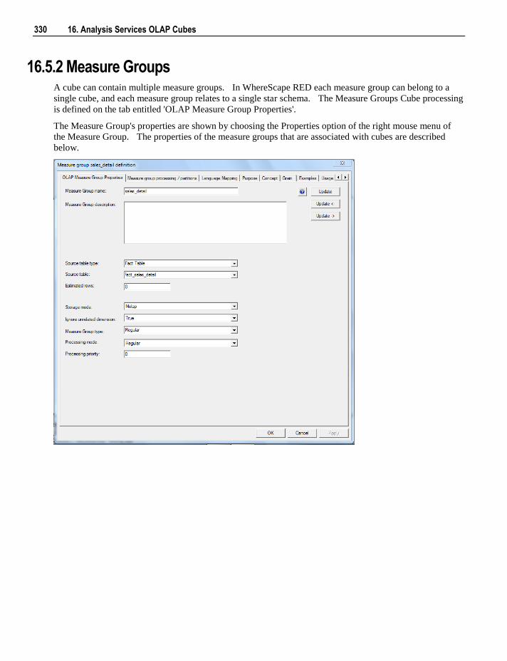
330 16. Analysis Services OLAP Cubes
16.5.2 Measure Groups A cube can contain multiple measure groups. In WhereScape RED each measure group can belong to a
single cube, and each measure group relates to a single star schema. The Measure Groups Cube processing
is defined on the tab entitled 'OLAP Measure Group Properties'.
The Measure Group's properties are shown by choosing the Properties option of the right mouse menu of
the Measure Group. The properties of the measure groups that are associated with cubes are described
below.
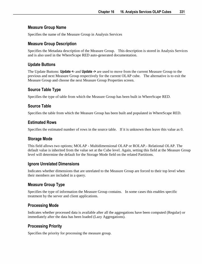
Chapter 16 16. Analysis Services OLAP Cubes 331
Measure Group Name
Specifies the name of the Measure Group in Analysis Services
Measure Group Description
Specifies the Metadata description of the Measure Group. This description is stored in Analysis Services
and is also used in the WhereScape RED auto-generated documentation.
Update Buttons
The Update Buttons: Update <- and Update -> are used to move from the current Measure Group to the
previous and next Measure Group respectively for the current OLAP cube. The alternative is to exit the
Measure Group and choose the next Measure Group Properties screen.
Source Table Type
Specifies the type of table from which the Measure Group has been built in WhereScape RED.
Source Table
Specifies the table from which the Measure Group has been built and populated in WhereScape RED.
Estimated Rows
Specifies the estimated number of rows in the source table. If it is unknown then leave this value as 0.
Storage Mode
This field allows two options; MOLAP - Multidimensional OLAP or ROLAP.- Relational OLAP. The
default value is inherited from the value set at the Cube level. Again, setting this field at the Measure Group
level will determine the default for the Storage Mode field on the related Partitions.
Ignore Unrelated Dimensions
Indicates whether dimensions that are unrelated to the Measure Group are forced to their top level when
their members are included in a query.
Measure Group Type
Specifies the type of information the Measure Group contains. In some cases this enables specific
treatment by the server and client applications.
Processing Mode
Indicates whether processed data is available after all the aggregations have been computed (Regular) or
immediately after the data has been loaded (Lazy Aggregations).
Processing Priority
Specifies the priority for processing the measure group.
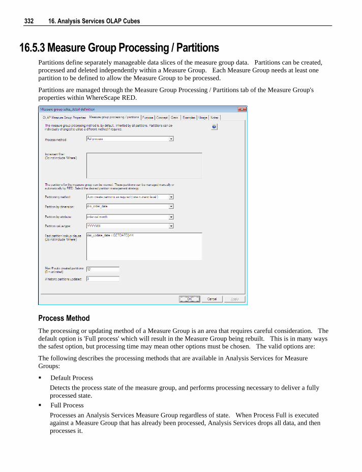
332 16. Analysis Services OLAP Cubes
16.5.3 Measure Group Processing / Partitions Partitions define separately manageable data slices of the measure group data. Partitions can be created,
processed and deleted independently within a Measure Group. Each Measure Group needs at least one
partition to be defined to allow the Measure Group to be processed.
Partitions are managed through the Measure Group Processing / Partitions tab of the Measure Group's
properties within WhereScape RED.
Process Method
The processing or updating method of a Measure Group is an area that requires careful consideration. The
default option is 'Full process' which will result in the Measure Group being rebuilt. This is in many ways
the safest option, but processing time may mean other options must be chosen. The valid options are:
The following describes the processing methods that are available in Analysis Services for Measure
Groups:
Default Process
Detects the process state of the measure group, and performs processing necessary to deliver a fully
processed state.
Full Process
Processes an Analysis Services Measure Group regardless of state. When Process Full is executed
against a Measure Group that has already been processed, Analysis Services drops all data, and then
processes it.
Chapter 16 16. Analysis Services OLAP Cubes 333
Incremental Process
Adds newly available fact data and process only to the relevant partitions. In order to use this option
you must set the 'incremental filter' field with a statement that will result in only new data being
selected. Failure to do so will result in duplicated data in the cube. In many data warehouses a fact
table undergoes changes to the data as well as the addition of new data, and so the incremental update
option is not possible. A validation regime should be put in place to compare cube data to the fact data
if incremental is used. This validation regime should be used to notify the administrator in the event
that duplicate data is inserted into the cube.
Update Data
Processes data only without building aggregations or indexes. If there is data in the partitions, it will
be dropped before re-populating the partition with source data. This processing option is supported for
dimensions, cubes, measure groups, and partitions.
Build Structure
If the cube is unprocessed, Analysis Services will process, if it is necessary, all the cube's dimensions.
After that, Analysis Services will create only cube definitions. The build structure option just builds
the cube structure without populating it. This can be useful if you have a very large cube and want to
validate the design.
Increment Filter
If an incremental processing option is chosen then a filter statement must be selected to only return those
rows that are to be added to the Measure Group. As mentioned above, care must be taken when using
incremental updates. For example, if the Measure Group is accidentally processed twice and the filter is
based on date, then duplicate data will be inserted into the Measure Group without any warning.
Partitioning
Partitioning is useful for handling large datasets where it is impractical to reprocess the entire Measure
Group. In such a case the full process option would probably be chosen but only selected partitions would
be processed. See the section on partitioning for more information. The default process will perform a
full process on the first pass followed by incremental updates on subsequent processing runs. Care should
be taken when choosing default for the cube.
Partitioning Method
Three options are provided for handling Measure Group partitions. They are:
1 One partition only
When this option is selected the partition information for the Measure Group is ignored and one
partition is created and processed for the Measure Group. This would be the normal situation unless
performance issues require an alternate strategy.
2 Manually managed multiple partitions
With this option the partition information stored for the Measure Group is used in the creation and
processing of the Measure Group.
3 Automatic partition handling
This option is available if the Measure Group is to be partitioned by one numeric value. The
partitioning should preferably be on something like day, month or year. (i.e. YYYY, YYYYMM or
YYYYDDD). If this option is chosen together with one of the date formats described above, then
WhereScape RED will automatically create partitions as required and process only those partitions that
are marked for processing.
334 16. Analysis Services OLAP Cubes
Partition by Dimension
This field is only available if automatic partition handling is chosen. Select the dimension in the Measure
Group that we will partition by. This would normally be a date dimension.
Partition by Attribute
This field is only available if automatic partition handling is chosen. Select the attribute that we are to
partition by. This would normally be a year or maybe a month level. (e.g. cal_year, fin_year from the
WhereScape date dimension).
Partition by Value Type
This field is only available if automatic partition handling is chosen. Select the type of level we are dealing
with. Choose YYYY for a year partition and YYYYMM for a month partition. This format must
correspond with the column in the date dimension. WhereScape RED only supports partitioning by Year,
Quarter, month or day.
Fact Partition Lookup Clause
This field is only available if automatic partition handling is chosen. In order to know when to create a
new partition WhereScape RED executes a query against the fact table and the date dimension to acquire
each unique period. When dealing with a large fact table, such a query may take a long time to complete.
This field can be used to include the components of the 'Where' clause to restrict the amount of data
examined. For example we may enter 'dss_update_time < GETDATE()-14' to only look at fact table
records that have been inserted or updated in the last 14 days. This should still allow us to catch any new
partitions and add them. The first time a cube is converted to auto partitioning handling, a full pass of the
fact table should occur to allow inclusion of every partition. This field should therefore only be populated
once the cube has been initially built with all partitions intact.
Max Number of Auto Created Partitions
This field is only available if automatic partition handling is chosen. You can specify an upper limit for
automatically created partitions. The default is zero, or no limit. This limit may be useful if your source
system can get erroneous data. If set, then the processing of the Measure Group will fail if a new partition
will exceed the counter.
Number of Historic Partitions Updated
This field is only available if automatic partition handling is chosen. This field allows you to restrict the
partition updating to the latest nnn partitions. If for example, we were partitioning by year and we set this
value to 2, we would process the current and previous years only. WhereScape RED turns off partition
processing after it does a partition update, so the first pass will still update all partitions.
To Display Measure Groups
To display a list of measure groups defined against a cube, right click on a cube and choose Display
Measure Groups.
To Add a Measure Group
To add a measure group, display the measure groups in the middle pane and either:
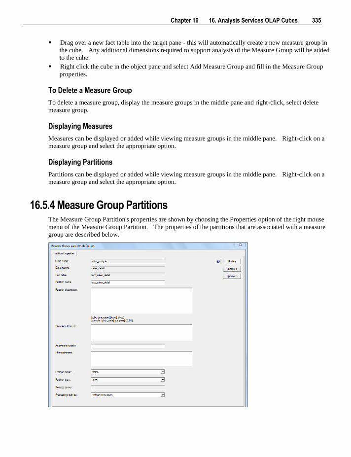
Chapter 16 16. Analysis Services OLAP Cubes 335
Drag over a new fact table into the target pane - this will automatically create a new measure group in
the cube. Any additional dimensions required to support analysis of the Measure Group will be added
to the cube.
Right click the cube in the object pane and select Add Measure Group and fill in the Measure Group
properties.
To Delete a Measure Group
To delete a measure group, display the measure groups in the middle pane and right-click, select delete
measure group.
Displaying Measures
Measures can be displayed or added while viewing measure groups in the middle pane. Right-click on a
measure group and select the appropriate option.
Displaying Partitions
Partitions can be displayed or added while viewing measure groups in the middle pane. Right-click on a
measure group and select the appropriate option.
16.5.4 Measure Group Partitions The Measure Group Partition's properties are shown by choosing the Properties option of the right mouse
menu of the Measure Group Partition. The properties of the partitions that are associated with a measure
group are described below.
336 16. Analysis Services OLAP Cubes
Cube name
The name of the cube that the partition belongs to.
Data source
The data source for the partitions. This will be inherited from the cube and cannot be changed. You cannot
have partitions with different data sources or different fact tables in WhereScape RED. If you need to
support either scenario then the partition must be created directly within Analysis Services. In such a case it
can still be managed in terms of processing through WhereScape RED.
Fact table
The fact table that the data is derived from.This is inherited from the cube and cannot be changed. See the
notes above under data source.
Update Buttons
The Update Buttons: Update <- and Update -> are used to move from the current Measure Group Partition to
the previous and next Measure Group Partition respectively for the current Measure Group. The
alternative is to exit the Measure Group Partition and choose the next Measure Group Partition Properties
screen.
Partition name
Where only one partition exists it is normally given the same name as the cube. If manually creating then a
unique name must be assigned for each partition. If auto partitioning is chosen then WhereScape RED will
use the cube name plus the level value to make the partition name.
Partition description
A description of the partition for documentation purposes.
Data slice formula
This field defines the range of data stored in the partition. It is a very simplified version of what can be done
in Analysis Services. If a more complex partitioning algorithm is required then the partition will need to be
created in Analysis Services. The format for the formula is as follows:
The brackets must surround each name and a full stop must separate the three parts of the formula. For
example a cube that is partitioned by year on its date dimension would have the following formula for the
2003 year. [dim_date].[cal_year].[2003]
Aggregation prefix
By default any cube aggregation will be prefixed with the partition name. An alternate name can be entered
here. See Analysis Services for more details.
Filter statement
Not implemented.
Storage mode
Chapter 16 16. Analysis Services OLAP Cubes 337
This field allows two options; MOLAP - Multidimensional OLAP or ROLAP.- Relational OLAP. This
determines how the OLAP cube is processed. The default value is inherited from the value set at the
Measure Group level.
Partition type
The partition can be either Local or Remote. Local means that the partition resides on the same Analysis
Services server as the cube. If Remote is chosen than a server must be specified where the partition will be
located.
Remote server
If a Remote partition then the name of the remote Analysis Services server must be entered here.
Processing method
A partition is either enabled for processing or disabled. This field can be set to Always process or Never
process. If left as default and in automatic mode then WhereScape RED will disable the processing once the
partition has been aged out.
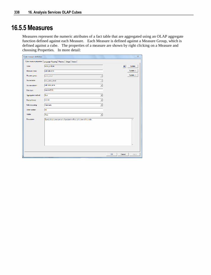
338 16. Analysis Services OLAP Cubes
16.5.5 Measures Measures represent the numeric attributes of a fact table that are aggregated using an OLAP aggregate
function defined against each Measure. Each Measure is defined against a Measure Group, which is
defined against a cube. The properties of a measure are shown by right clicking on a Measure and
choosing Properties. In more detail:
Chapter 16 16. Analysis Services OLAP Cubes 339
Cube
A Read Only field that indicates against which OLAP Cube the measure is defined.
Measure Name
Specifies the Analysis Services name defined for the measure.
Measure Group
Specifies against which Measure Group the Measure is defined. This is related to the fact table of which
the Measure is an attribute.
Update Buttons
The Update Buttons: Update <- and Update -> are used to move from the current Measure to the previous
and next Measure respectively for the current OLAP Cube Measure Group. The alternative is to exit the
Measure and choose the next Measure Properties screen.
Source Table
A read only field that indicates the fact table that is related to the Measure Group.
Source Column
Specifies from which numeric attribute of the underlying fact table the Measure is built. This is a drop
down list populated from REDs metadata definition of the fact table associated with the Measure Group
above.
Data Type
Specifies the data type used by Analysis Services. The data type specified for this property is inherited
from the fact table attribute defined in WhereScape RED metadata but can be different (typically a larger
data type is used in the cube to cope with the larger numbers generated by aggregating the source data).
Aggregation Method
Specifies the OLAP function used to aggregate measure values. The default options are:
Sum
Count
Distinct Count - only one distinct count is allowed per Measure Group and can have query performance
implications.
Min - Minimum
Max - Maximum
Display Format
Specifies the format used by clients when displaying the measure value.
Null Processing
340 16. Analysis Services OLAP Cubes
Specifies the processing null values. Setting this property to Automatic means that Analysis Services uses
default behavior.
Order number
The order in which the measures appear in the cube is dictated by their order number.
Visible
Measures are normally visible, but some measures used in calculations may be hidden. In such a case clear
this check box.
Description
A description of the measure which is stored in the cube. This description will by default be acquired from
the source column.
To View measures
The measures can be viewed by clicking on an OLAP Cube in the left pane which will display the measures
in the middle pane.
To Add a New Measure
To add a new measure, view the measures in the middle pane, right-click in the middle pane and select add
measure. This can also be done when viewing measure groups in the middle pane. Alternatively to create
measure which is very similar to an existing measure, view the measures in the middle pane and right-click,
select "copy measure". The same dialog box appears as for "add measure" with most of the fields filled in.
Notice that the measure name has the suffix "- Copy". Change the name in the Measure Name field and
make any other alterations and click OK.
To Delete a measure
Display the measures in the middle pane, select the measure to delete, right-click and select Delete.
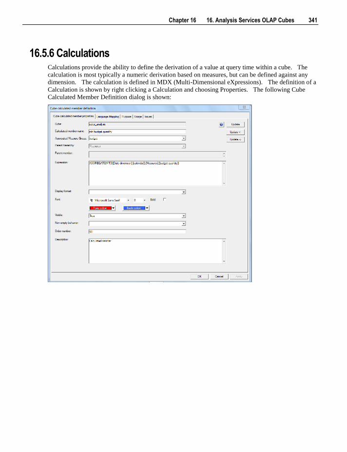
Chapter 16 16. Analysis Services OLAP Cubes 341
16.5.6 Calculations Calculations provide the ability to define the derivation of a value at query time within a cube. The
calculation is most typically a numeric derivation based on measures, but can be defined against any
dimension. The calculation is defined in MDX (Multi-Dimensional eXpressions). The definition of a
Calculation is shown by right clicking a Calculation and choosing Properties. The following Cube
Calculated Member Definition dialog is shown:
342 16. Analysis Services OLAP Cubes
Cube
A Read Only field that indicates against which OLAP Cube the Calculation is defined.
Calculated Member Name
Specifies the Analysis Services name defined for the Calculation.
Associated Measure Group
Specifies against which Measure Group the Measure is defined. This is related to the fact table of which
the Measure is an attribute.
Note: SSAS 2008+ uses the property "Associated Measure Group" but previous versions of SSAS do not
and can result in errors when creating the cube. It is possible to set this attribute in RED to "(Undefined)"
for previous versions of RED, but this is not necessary for the current version of RED as this attribute will
only be used when appropriate.
Update Buttons
The Update Buttons: Update <- and Update -> are used to move from the current Calculation to the previous
and next Calculation respectively for the current OLAP Cube. The alternative is to exit the Calculation and
choose the next Calculation Properties screen.
Parent Hierarchy
Specifies the dimension hierarchy in which the calculation is created.
Parent Member
If the Parent Hierarchy is anything other than Measures, then this value specifies the parent member for the
calculation.
Expression
Specifies the MDX expression that defines the calculation.
Display Format
Specifies the format used by clients when displaying the measure value.
Visible
Specifies whether the calculation is visible to client tools.
Non Empty Behavior
Determines the non-empty behavior associated with the calculation
Order Number
The create order of the member in the dimension hierarchy.
Description
Chapter 16 16. Analysis Services OLAP Cubes 343
A business description of the Calculation that is used to populate WhereScape RED documentation.
To View Calculations
To view the list of calculations (sometimes called a calculated measure), right-click on an OLAP Cube in
the left pane and select Display Calculations.
To Add a Calculation
1 To add a calculation, right-click on an OLAP Cube in the left pane and select "Add Calculation". This
can also be achieved by displaying calculations in the middle pane, right-clicking and selecting "add
calculation". Fill out the dialog box with the relevant details.
2 To create a calculation that is similar to an existing calculation, display the calculations in the middle
pane and select "copy Calculation". The same dialog box appears as for "add calculation" with most of
the fields filled in. Notice that the calculated member name has the suffix "- Copy". Change the
name in the Measure Name field and make any other alterations and click OK.
To Delete a calculation
Display the calculations in the middle pane, select the calculation to delete, right-click and select Delete.
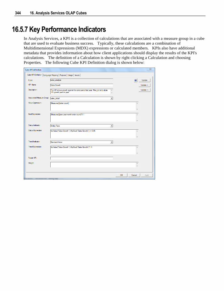
344 16. Analysis Services OLAP Cubes
16.5.7 Key Performance Indicators In Analysis Services, a KPI is a collection of calculations that are associated with a measure group in a cube
that are used to evaluate business success. Typically, these calculations are a combination of
Multidimensional Expressions (MDX) expressions or calculated members. KPIs also have additional
metadata that provides information about how client applications should display the results of the KPI's
calculations. The definition of a Calculation is shown by right clicking a Calculation and choosing
Properties. The following Cube KPI Definition dialog is shown below:
Chapter 16 16. Analysis Services OLAP Cubes 345
Cube
A Read Only field that indicates against which OLAP Cube the KPI is defined.
KPI Name
Specifies the name of the KPI defined in Analysis Services.
Description
A business description of the KPI that is used to populate WhereScape RED documentation.
Update Buttons
The Update Buttons: Update <- and Update -> are used to move from the current KPI to the previous and
next KPI respectively for the current OLAP Cube. The alternative is to exit the KPI and choose the next
KPI Properties screen.
Associated Measure Group
Specifies the Measure Group against which the KPI is defined.
Value
An MDX numeric expression that returns the actual value of the KPI.
Goal
An MDX numeric expression or a calculation that returns the target value of the KPI.
Status
An MDX expression that represents the state of the KPI at a specified point in time.
The status MDX expression should return a normalized value between -1 and 1. Values equal to or less
than -1 will be interpreted as "bad" or "low." A value of zero (0) is interpreted as "acceptable" or "medium."
Values equal to or greater than 1 will be interpreted as "good" or "high."
An unlimited number of intermediate values can optionally be returned and can be used to display any
number of additional states, if supported by the client application.
Status Indicator
A visual element that provides a quick indication of the status of a KPI. The display of the element is
determined by the value of the MDX expression that evaluates status.
Trend
An MDX expression that evaluates the value of the KPI over time. The trend can be any time-based
criterion that is useful in a specific business context.
The trend MDX expression enables a business user to determine whether the KPI is improving over time or
degrading over time.
346 16. Analysis Services OLAP Cubes
Trend Indicator
A visual element that provides a quick indication of the trend for a KPI. The display of the element is
determined by the value of the MDX expression that evaluates trend.
Display Folder
The folder in which the KPI will appear when a user is browsing the cube.
Parent KPI
A reference to an existing KPI that uses the value of the child KPI as part of computation of the parent KPI.
Sometimes, a single KPI will be a computation that consists of the values for other KPIs. This property
facilitates the correct display of the child KPIs underneath the parent KPI in client applications.
Current Time Member
An MDX expression that returns the member that identifies the temporal context of the KPI.
Weight
An MDX numeric expression that assigns a relative importance to a KPI. If the KPI is assigned to a parent
KPI, the weight is used to proportionally adjust the results of the child KPI value when calculating the value
of the parent KPI.
To View KPIs
To view the list of KPIs, right-click on an OLAP Cube in the left pane and select "Display KPIs".
To Add a KPI
1 To add a calculation, right-click on an OLAP Cube in the left pane and select "Add KPI". This can
also be achieved by displaying KPIs in the middle pane, right-clicking and selecting "Add KPI". Fill
out the dialog box with the relevant details.
2 To create a KPI that is similar to an existing KPI, display the KPIs in the middle pane and select "Copy
KPI". The same dialog box appears as for "Add KPI" with most of the fields filled in. Notice that the
KPI name has the suffix "- Copy". Change the name in the KPI Name field and make any other
alterations and click OK.
To Delete a KPI
Display the KPIs in the middle pane, select the KPI to delete, right-click and select Delete.
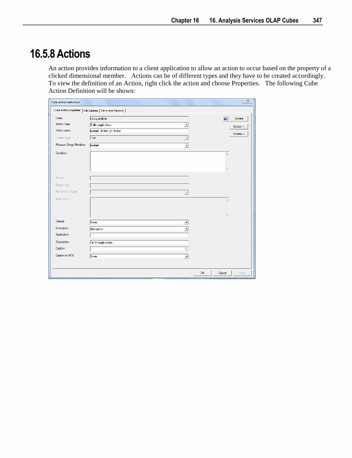
Chapter 16 16. Analysis Services OLAP Cubes 347
16.5.8 Actions An action provides information to a client application to allow an action to occur based on the property of a
clicked dimensional member. Actions can be of different types and they have to be created accordingly.
To view the definition of an Action, right click the action and choose Properties. The following Cube
Action Definition will be shown:
348 16. Analysis Services OLAP Cubes
Cube
A Read Only field that indicates against which OLAP Cube the Calculation is defined.
Action Type
Actions can be of the following types:
Drill through actions which return the set of rows that represents the underlying data of the selected
cells of the cube where the action occurs. When this option is chosen an additional tab is enabled that
allows drill through columns to be chosen.
Reporting actions which return a report from Reporting Services that is associated with the selected
section of the cube where the action occurs.
Standard actions (Action), which return the action element (URL, HTML, DataSet, RowSet, and other
elements) that is associated with the selected section of the cube where the action occurs.
The action type chosen determines which action specific fields are enabled within the dialog.
Action Name
Defines the name of the Action in the Cube.
Update Buttons
The Update Buttons: Update <- and Update -> are used to move from the current Action to the previous and
next Action respectively for the current OLAP Cube. The alternative is to exit the Action and choose the
next Action Properties screen.
Target Type
Select the object to which the action is attached. Generally, in client applications, the action is displayed
when end users select the target object; however, the client application determines which end-user operation
displays actions. For Target type, select from the following objects:
Attribute members
Cells
Cube
Dimension members
Hierarchy
Hierarchy members
Level
Level members
Target Object
The cube object of the designated target type against which the action is defined.
Condition
Chapter 16 16. Analysis Services OLAP Cubes 349
Specify an optional Multidimensional Expressions (MDX) expression that resolves to a Boolean value. If
the value is True, the action is performed on the specified target. If the value is False, the action is not
performed.
Report Action: Server
The name of the computer running report server.
Report Action: Report Path
The path exposed by report server.
Content Type
Select the type of action. The following table summarizes the available types.
Data Set - Retrieves a dataset
Proprietary - Performs an operation by using an interface other than those listed in this table.
Row Set - Retrieves a rowset.
Statement - Runs an OLE DB command.
URL - Displays a page in an Internet Browser.
Expression
Specifies the parameters that are passed when the action is run. The syntax must evaluate to a string, and
you must include an expression written in MDX. MDX expressions are evaluated before the parameters
are passed.
Default
An additional true/false drop list is enabled for Drill through actions. This gets or sets the current
DrillThroughAction as the default action when multiple drillthrough actions are defined. This is important
for users of Excell 2007 to browse the Olap Cube because Excell will only invoke the Drill through Action
marked as the default.
Invocation
Specifies how the action is run. Interactive, the default, specifies that the action is run when a user
accesses an object. The possible settings are:
Batch
Interactive
On Open
Application
Describes the application of the action.
URL
The URL opened by the action.
350 16. Analysis Services OLAP Cubes
Description
Describes the action.
Caption
Provides a caption that is displayed for the action.
Caption is MDX
If the caption is MDX, specify True, if not specify False.
To View Actions
To view the list of Actions, right-click on an OLAP Cube in the left pane and select "Display Actions".
To Add an Action
1 To add an Action, right-click on an OLAP Cube in the left pane and select "Add Action". This can
also be achieved by displaying Actions in the middle pane, right-clicking and selecting "Add Action".
Fill out the dialog box with the relevant details.
2 To create an Action that is similar to an existing Action, display the Actions in the middle pane and
select "Copy Action". The same dialog box appears as for "Add Action" with most of the fields filled
in. Notice that the Action name has the suffix "- Copy". Change the name in the Action Name field
and make any other alterations and click OK.
To Delete an Action
Display the Actions in the middle pane, select the Action to delete, right-click and select Delete.
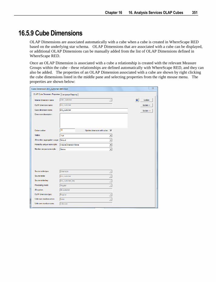
Chapter 16 16. Analysis Services OLAP Cubes 351
16.5.9 Cube Dimensions OLAP Dimensions are associated automatically with a cube when a cube is created in WhereScape RED
based on the underlying star schema. OLAP Dimensions that are associated with a cube can be displayed,
or additional OLAP Dimensions can be manually added from the list of OLAP Dimensions defined in
WhereScape RED.
Once an OLAP Dimension is associated with a cube a relationship is created with the relevant Measure
Groups within the cube - these relationships are defined automatically with WhereScape RED, and they can
also be added. The properties of an OLAP Dimension associated with a cube are shown by right clicking
the cube dimensions listed in the middle pane and selecting properties from the right mouse menu. The
properties are shown below:
352 16. Analysis Services OLAP Cubes
Internal Dimension Name
A read only field displaying the name of the OLAP Dimension in WhereScape RED.
OLAP Dimension Name
Specifies the name of the OLAP Dimension as a Dimension in Analysis Services.
Cube Dimension Name
Specifies the exposed name of the Dimension when associated with a cube (this can be different from the
OLAP Dimension Name).
Update Buttons
The Update Buttons: Update <- and Update -> are used to move from the current OLAP Dimension to the
previous and next OLAP Dimension respectively for the current OLAP Cube. The alternative is to exit the
OLAP Dimension and choose the next OLAP Dimension Properties screen.
Dimension Description
A description of the dimension when associated with the cube.
Order Number
The order number.
All member aggregation usage
Specifies how aggregations will be designed by the BIDS Storage Design Wizard if it is used to design cube
aggregations.
Hierarchy unique name style
Indicates whether the dimension name will be included in the name of the hierarchies. If set to Default
then the system will apply a default behavior and will include the dimension name in the case where there is
more than one usage of the same dimension.
Member unique name style
Indicates how member unique names will be formed.
Other Read only fields that are displayed in this dialog are configurable against the OLAP Dimensions'
properties and cannot be changed in this dialog, including:
Source Table Type
Source Table
Source Table Key
Processing Mode
All caption
OLAP Dimension Type
Unknown Member Action
Unknown Member Name
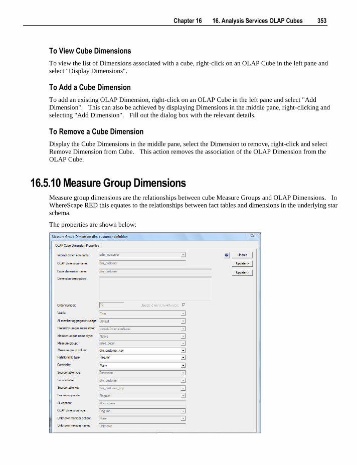
Chapter 16 16. Analysis Services OLAP Cubes 353
To View Cube Dimensions
To view the list of Dimensions associated with a cube, right-click on an OLAP Cube in the left pane and
select "Display Dimensions".
To Add a Cube Dimension
To add an existing OLAP Dimension, right-click on an OLAP Cube in the left pane and select "Add
Dimension". This can also be achieved by displaying Dimensions in the middle pane, right-clicking and
selecting "Add Dimension". Fill out the dialog box with the relevant details.
To Remove a Cube Dimension
Display the Cube Dimensions in the middle pane, select the Dimension to remove, right-click and select
Remove Dimension from Cube. This action removes the association of the OLAP Dimension from the
OLAP Cube.
16.5.10 Measure Group Dimensions Measure group dimensions are the relationships between cube Measure Groups and OLAP Dimensions. In
WhereScape RED this equates to the relationships between fact tables and dimensions in the underlying star
schema.
The properties are shown below:
354 16. Analysis Services OLAP Cubes
Internal Dimension Name
A read only field displaying the name of the OLAP Dimension in WhereScape RED.
OLAP Dimension Name
A read only field displaying the name of the OLAP Dimension as a Dimension in Analysis Services.
Cube Dimension Name
A read only field displaying the name of the Dimension when associated with a cube (this can be different
from the OLAP Dimension Name).
Update Buttons
The Update Buttons: Update <- and Update -> are used to move from the current OLAP Measure Group
Dimension to the previous and next OLAP Measure Group Dimension respectively for the current OLAP
Cube. The alternative is to exit the OLAP Measure Group Dimension and choose the next OLAP Measure
Group Dimension Properties screen.
Dimension Description
A description of the dimension when it is associated with the cube.
Order Number
The order number.
Update dimension with Cube
A read only check box showing whether the dimension is processed when the cube is processed.
Visible
A read only field displaying the visibility of the dimension on the cube.
All member aggregation usage
A read only field displaying how aggregations will be designed by the BIDS Storage Design Wizard if it is
used to design cube aggregations.
Hierarchy unique name style
A read only field which indicates whether the dimension name will be included in the name of the
hierarchies.
Member unique name style
A read only field which indicates how member unique names will be formed. A read only field.
Measure group
A read only field displaying the Measure Group which is being referenced by the Measure Group
Dimension relationship.
Chapter 16 16. Analysis Services OLAP Cubes 355
Measure group column
Specifies which fact table key joins to the dimension key.
Relationship type
Defines the relationship type for the relationship between the Dimension and Measure Group. In
WhereScape RED this option can be Regular, which means that the relationship is based on a dimension
key join, or No Relationship between the Measure Group and Dimension.
Cardinality
Indicates whether the measure group has a many to one or one to one relationship with the dimension.
Source Table Type
A read only field that displays the type of table from which the OLAP Dimension was created.
Source Table
A read only field that displays the name of the table from which the OLAP Dimension was created.
Source Table Key
A read only field that displays the key (typically the primary key) that relates the dimension to the fact in
the underlying star schema.
Processing Mode
A read only field that indicates whether processed data is available after all aggregations have been
computed or immediately after the data has been loaded.
All Caption
A read only field that displays the name of the (All) member. This applies to all hierarchies in the
dimension that have an (All) member.
OLAP Dimension Type
A read only field that displays the type of information contained by the dimension.
Unknown member Action
A read only field that displays the existence of an Unknown member and whether that member is visible or
hidden.
Unknown Member Name
A read only field that displays the caption for the unknown member.
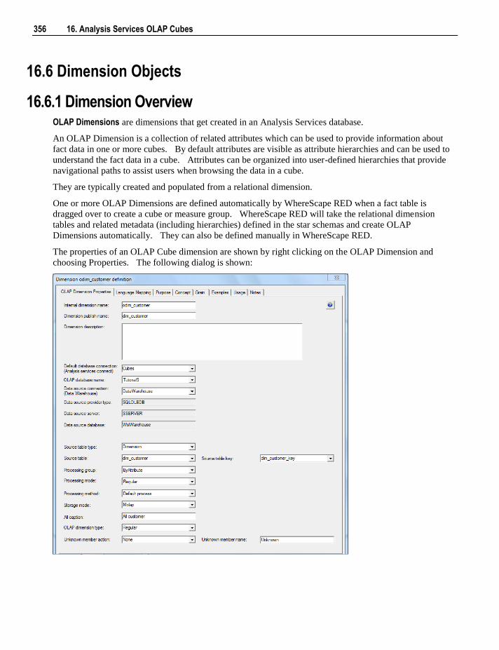
356 16. Analysis Services OLAP Cubes
16.6 Dimension Objects
16.6.1 Dimension Overview OLAP Dimensions are dimensions that get created in an Analysis Services database.
An OLAP Dimension is a collection of related attributes which can be used to provide information about
fact data in one or more cubes. By default attributes are visible as attribute hierarchies and can be used to
understand the fact data in a cube. Attributes can be organized into user-defined hierarchies that provide
navigational paths to assist users when browsing the data in a cube.
They are typically created and populated from a relational dimension.
One or more OLAP Dimensions are defined automatically by WhereScape RED when a fact table is
dragged over to create a cube or measure group. WhereScape RED will take the relational dimension
tables and related metadata (including hierarchies) defined in the star schemas and create OLAP
Dimensions automatically. They can also be defined manually in WhereScape RED.
The properties of an OLAP Cube dimension are shown by right clicking on the OLAP Dimension and
choosing Properties. The following dialog is shown:
Chapter 16 16. Analysis Services OLAP Cubes 357
Internal Dimension Name
Specifies the name of the dimension in WhereScape RED.
Dimension Publish Name
Specifies the name of the dimension as created in Analysis Services.
Dimension Description
A business description of the OLAP Dimension for use in documentation - this description also gets created
in the analysis services metadata.
Default database connection and OLAP Database Name
The WhereScape RED connection that is an OLAP connection to an analysis services server. These fields
only need to be populated when the OLAP Dimension needs to be created in Analysis Services separately
from a cube. If these fields are blank this dimension can only be created in the same Analysis Services
server and database as the related cubes when the cubes get created.
Data Source Connection
Defines the WhereScape RED connection that points to the relational dimensional table(s) used to populate
the OLAP Dimension - typically the Data Warehouse connection. When the connection is defined the
following read only fields are populated with the connection information:
Data Source Provider Type
Data Source Server
Data Source Database
Source Table Type
Specifies the type of table from which the OLAP Dimension was created.
Source Table
Specifies the name of the table from which the OLAP Dimension was created.
Source Table Key
Specifies the key (typically the primary key) that relates the dimension to the fact in the underlying star
schema.
Processing Group
Specifies the processing group for processing the dimension. This determines how much data is read into
memory during dimension processing at any one time.
Processing Mode
Indicates whether processed data is available after all aggregations have been computed (Regular) or
immediately after the data has been loaded (Lazy aggregations).
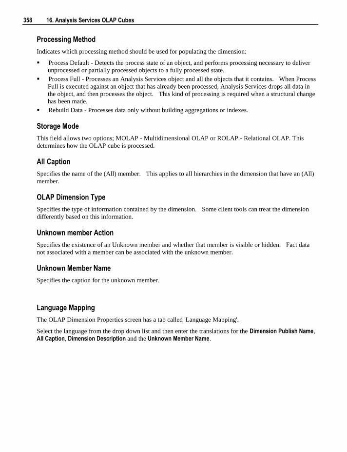
358 16. Analysis Services OLAP Cubes
Processing Method
Indicates which processing method should be used for populating the dimension:
Process Default - Detects the process state of an object, and performs processing necessary to deliver
unprocessed or partially processed objects to a fully processed state.
Process Full - Processes an Analysis Services object and all the objects that it contains. When Process
Full is executed against an object that has already been processed, Analysis Services drops all data in
the object, and then processes the object. This kind of processing is required when a structural change
has been made.
Rebuild Data - Processes data only without building aggregations or indexes.
Storage Mode
This field allows two options; MOLAP - Multidimensional OLAP or ROLAP.- Relational OLAP. This
determines how the OLAP cube is processed.
All Caption
Specifies the name of the (All) member. This applies to all hierarchies in the dimension that have an (All)
member.
OLAP Dimension Type
Specifies the type of information contained by the dimension. Some client tools can treat the dimension
differently based on this information.
Unknown member Action
Specifies the existence of an Unknown member and whether that member is visible or hidden. Fact data
not associated with a member can be associated with the unknown member.
Unknown Member Name
Specifies the caption for the unknown member.
Language Mapping
The OLAP Dimension Properties screen has a tab called 'Language Mapping'.
Select the language from the drop down list and then enter the translations for the Dimension Publish Name, All Caption, Dimension Description and the Unknown Member Name.
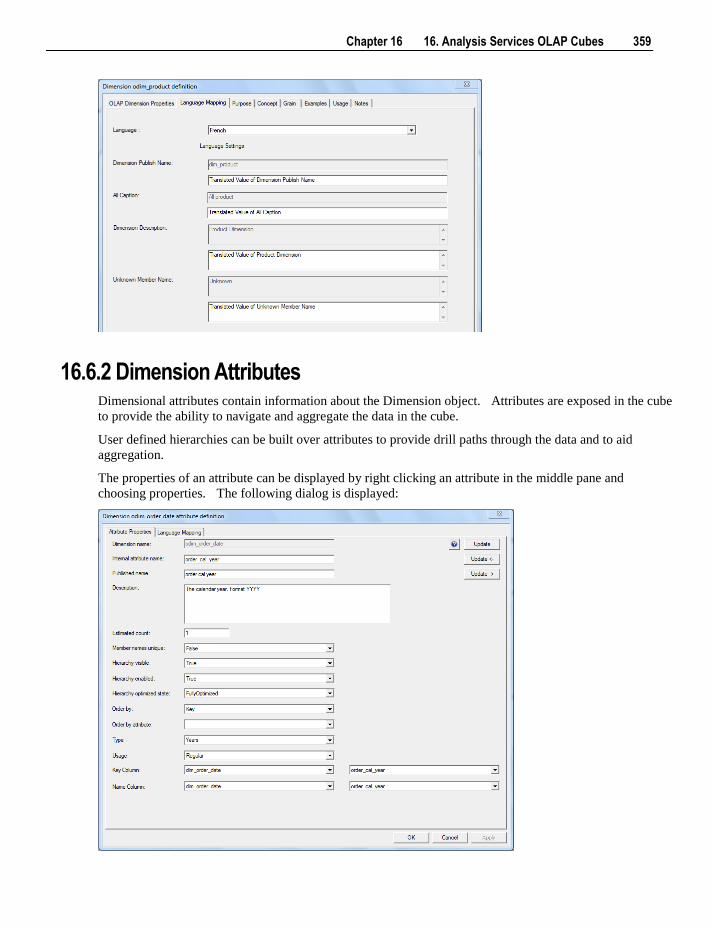
Chapter 16 16. Analysis Services OLAP Cubes 359
16.6.2 Dimension Attributes Dimensional attributes contain information about the Dimension object. Attributes are exposed in the cube
to provide the ability to navigate and aggregate the data in the cube.
User defined hierarchies can be built over attributes to provide drill paths through the data and to aid
aggregation.
The properties of an attribute can be displayed by right clicking an attribute in the middle pane and
choosing properties. The following dialog is displayed:
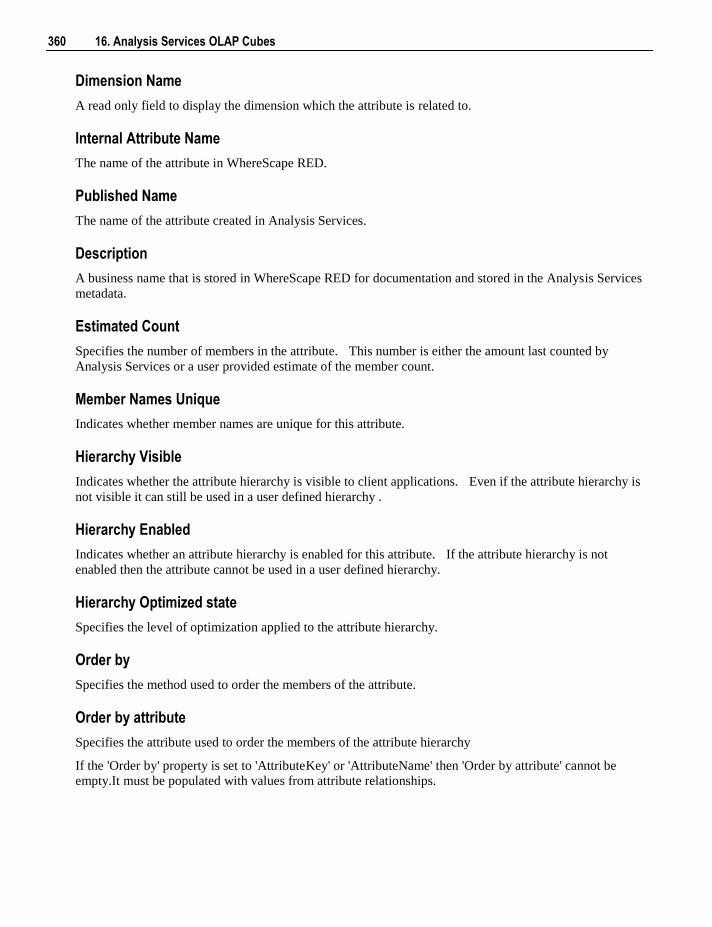
360 16. Analysis Services OLAP Cubes
Dimension Name
A read only field to display the dimension which the attribute is related to.
Internal Attribute Name
The name of the attribute in WhereScape RED.
Published Name
The name of the attribute created in Analysis Services.
Description
A business name that is stored in WhereScape RED for documentation and stored in the Analysis Services
metadata.
Estimated Count
Specifies the number of members in the attribute. This number is either the amount last counted by
Analysis Services or a user provided estimate of the member count.
Member Names Unique
Indicates whether member names are unique for this attribute.
Hierarchy Visible
Indicates whether the attribute hierarchy is visible to client applications. Even if the attribute hierarchy is
not visible it can still be used in a user defined hierarchy .
Hierarchy Enabled
Indicates whether an attribute hierarchy is enabled for this attribute. If the attribute hierarchy is not
enabled then the attribute cannot be used in a user defined hierarchy.
Hierarchy Optimized state
Specifies the level of optimization applied to the attribute hierarchy.
Order by
Specifies the method used to order the members of the attribute.
Order by attribute
Specifies the attribute used to order the members of the attribute hierarchy
If the 'Order by' property is set to 'AttributeKey' or 'AttributeName' then 'Order by attribute' cannot be
empty.It must be populated with values from attribute relationships.
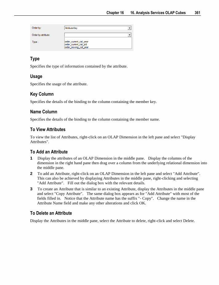
Chapter 16 16. Analysis Services OLAP Cubes 361
Type
Specifies the type of information contained by the attribute.
Usage
Specifies the usage of the attribute.
Key Column
Specifies the details of the binding to the column containing the member key.
Name Column
Specifies the details of the binding to the column containing the member name.
To View Attributes
To view the list of Attributes, right-click on an OLAP Dimension in the left pane and select "Display
Attributes".
To Add an Attribute
1 Display the attributes of an OLAP Dimension in the middle pane. Display the columns of the
dimension in the right hand pane then drag over a column from the underlying relational dimension into
the middle pane.
2 To add an Attribute, right-click on an OLAP Dimension in the left pane and select "Add Attribute".
This can also be achieved by displaying Attributes in the middle pane, right-clicking and selecting
"Add Attribute". Fill out the dialog box with the relevant details.
3 To create an Attribute that is similar to an existing Attribute, display the Attributes in the middle pane
and select "Copy Attribute". The same dialog box appears as for "Add Attribute" with most of the
fields filled in. Notice that the Attribute name has the suffix "- Copy". Change the name in the
Attribute Name field and make any other alterations and click OK.
To Delete an Attribute
Display the Attributes in the middle pane, select the Attribute to delete, right-click and select Delete.
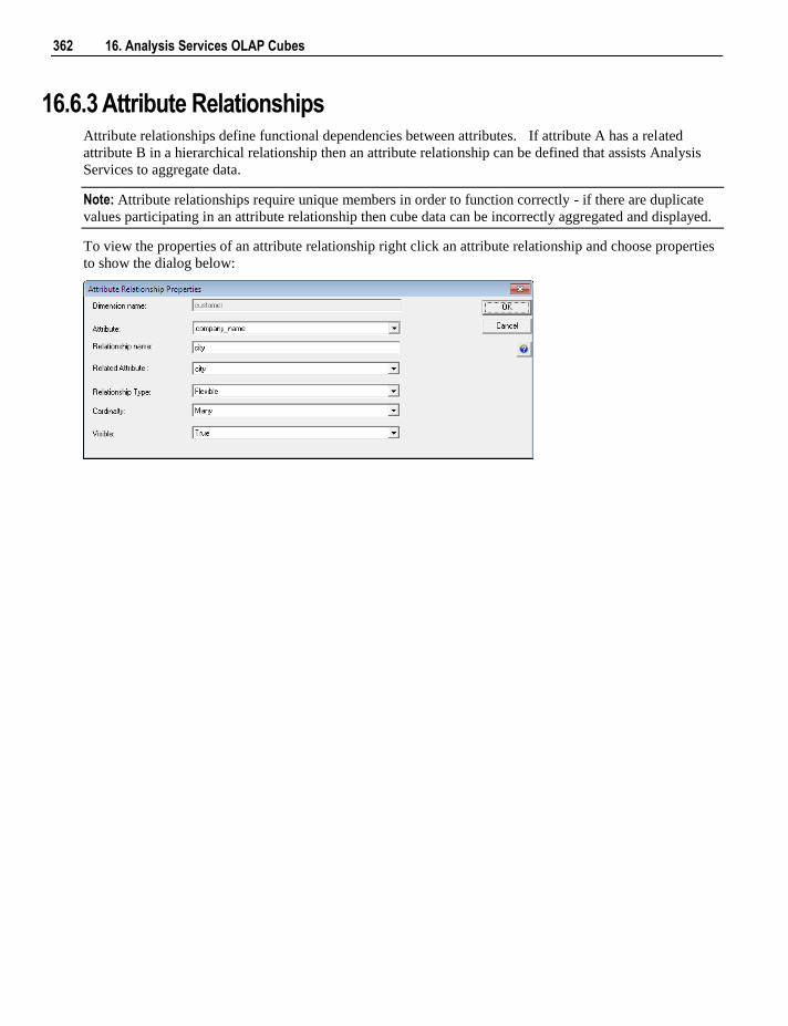
362 16. Analysis Services OLAP Cubes
16.6.3 Attribute Relationships Attribute relationships define functional dependencies between attributes. If attribute A has a related
attribute B in a hierarchical relationship then an attribute relationship can be defined that assists Analysis
Services to aggregate data.
Note: Attribute relationships require unique members in order to function correctly - if there are duplicate
values participating in an attribute relationship then cube data can be incorrectly aggregated and displayed.
To view the properties of an attribute relationship right click an attribute relationship and choose properties
to show the dialog below:
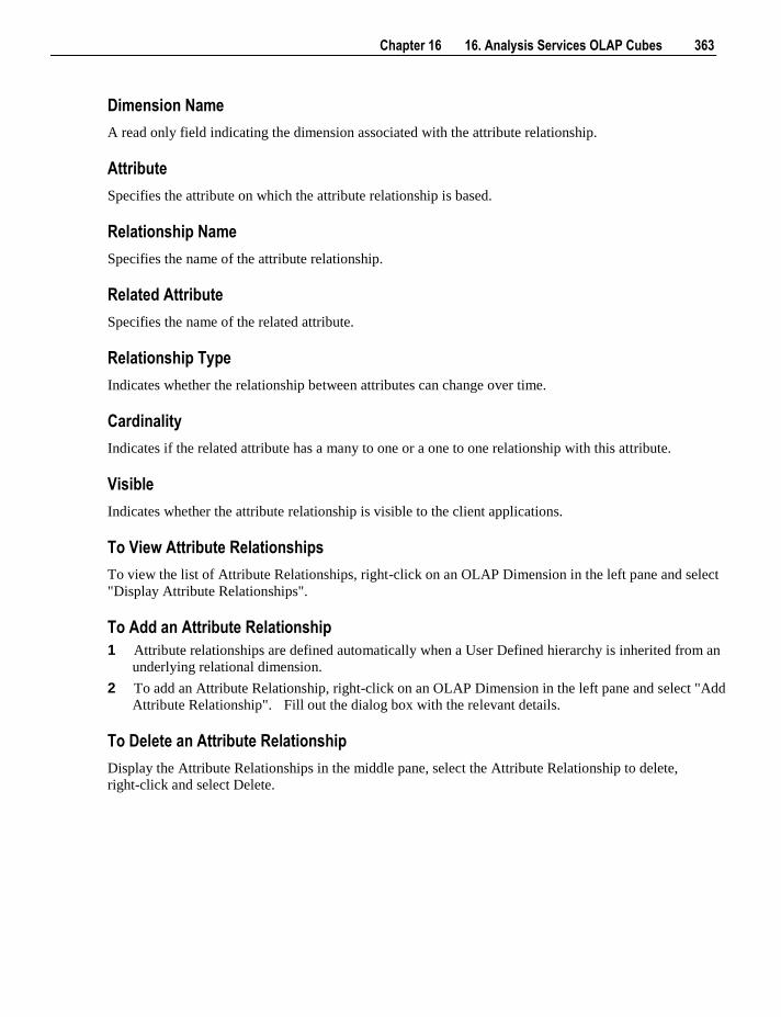
Chapter 16 16. Analysis Services OLAP Cubes 363
Dimension Name
A read only field indicating the dimension associated with the attribute relationship.
Attribute
Specifies the attribute on which the attribute relationship is based.
Relationship Name
Specifies the name of the attribute relationship.
Related Attribute
Specifies the name of the related attribute.
Relationship Type
Indicates whether the relationship between attributes can change over time.
Cardinality
Indicates if the related attribute has a many to one or a one to one relationship with this attribute.
Visible
Indicates whether the attribute relationship is visible to the client applications.
To View Attribute Relationships
To view the list of Attribute Relationships, right-click on an OLAP Dimension in the left pane and select
"Display Attribute Relationships".
To Add an Attribute Relationship
1 Attribute relationships are defined automatically when a User Defined hierarchy is inherited from an
underlying relational dimension.
2 To add an Attribute Relationship, right-click on an OLAP Dimension in the left pane and select "Add
Attribute Relationship". Fill out the dialog box with the relevant details.
To Delete an Attribute Relationship
Display the Attribute Relationships in the middle pane, select the Attribute Relationship to delete,
right-click and select Delete.
364 16. Analysis Services OLAP Cubes
16.6.4 Dimension Hierarchies User defined hierarchies define hierarchical relationships between related dimensional attributes (e.g.
Geographical or time based attributes). These related attributes are defined as levels within the hierarchy.
To view the properties of a user defined Hierarchy right click the Hierarchy and choose properties to show
the dialog below:
Chapter 16 16. Analysis Services OLAP Cubes 365
Dimension Name
A read only field indicating the dimension associated with the attribute relationship.
Internal Hierarchy Name
The name of the hierarchy within WhereScape RED.
Hierarchy Publish Name
The name of the hierarchy as created within Analysis Services.
Hierarchy Description
A business name that is stored in WhereScape RED for documentation and stored in the Analysis Services
metadata.
All Member Name
Specifies the name of the member in the All level
Allow duplicate Names
Indicates whether the members under a common parent can have the same name.
Member Keys Unique
Indicates whether member keys are unique for this hierarchy.
Member Names Unique
Indicates whether member names are unique for this hierarchy.
To view User Defined Hierarchies
To view the list of User Defined Hierarchies, right-click on an OLAP Dimension in the left pane and select
"Display Hierarchies".
To Add a User Defined Hierarchy
To add a User Defined Hierarchy, right-click on an OLAP Dimension in the left pane and select "Add
Hierarchy". Fill out the dialog box with the relevant details.
To Delete a User Defined Hierarchy
Display the User Defined Hierarchies in the middle pane, select the User Defined Hierarchy to delete,
right-click and select Delete.
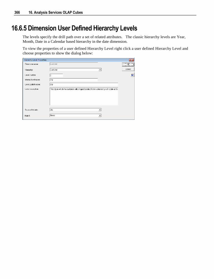
366 16. Analysis Services OLAP Cubes
16.6.5 Dimension User Defined Hierarchy Levels The levels specify the drill path over a set of related attributes. The classic hierarchy levels are Year,
Month, Date in a Calendar based hierarchy in the date dimension.
To view the properties of a user defined Hierarchy Level right click a user defined Hierarchy Level and
choose properties to show the dialog below:
Chapter 16 16. Analysis Services OLAP Cubes 367
Dimension Name
A read only field indicating the dimension associated with the attribute relationship.
Hierarchy
The User Defined Hierarchy that contains the level.
Level Number
The number of levels from the top most hierarchy level. These level numbers must start at 1 for the top
level and provide continuous numbering to the bottom level.
Internal Level Name
The name of the Level within WhereScape RED.
Level Publish Name
The name of the Level as created within Analysis Services.
Level Description
A business name that is stored in WhereScape RED for documentation and stored in the Analysis Services
metadata.
Source Attribute
Specifies the source attribute on which the level is based.
Hide If
Specifies which members are hidden. This property supports ragged hierarchies containing logical gaps
between members.
To View User Defined Hierarchy Levels
To view the list of User Defined Hierarchy Levels, right-click on an OLAP Dimension in the left pane and
select "Display Hierarchy Levels".
To Add a User Defined Hierarchy
1 To add a User Defined Hierarchy level, right-click on an OLAP Dimension in the left pane and select
"Add Hierarchy Level". Fill out the dialog box with the relevant details.
2 Alternatively right click on a User Defined Hierarchy in the middle pane and select "Add Hierarchy
Level". Fill out the dialog box with the relevant details.
To Delete a User Defined Hierarchy Level
Display the User Defined Hierarchy Levels in the middle pane, select the User Defined Hierarchy Level to
delete, right-click and select Delete.
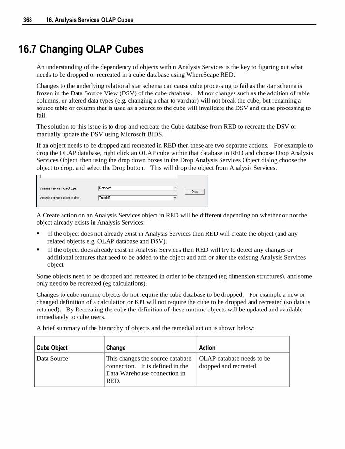
368 16. Analysis Services OLAP Cubes
16.7 Changing OLAP Cubes
An understanding of the dependency of objects within Analysis Services is the key to figuring out what
needs to be dropped or recreated in a cube database using WhereScape RED.
Changes to the underlying relational star schema can cause cube processing to fail as the star schema is
frozen in the Data Source View (DSV) of the cube database. Minor changes such as the addition of table
columns, or altered data types (e.g. changing a char to varchar) will not break the cube, but renaming a
source table or column that is used as a source to the cube will invalidate the DSV and cause processing to
fail.
The solution to this issue is to drop and recreate the Cube database from RED to recreate the DSV or
manually update the DSV using Microsoft BIDS.
If an object needs to be dropped and recreated in RED then these are two separate actions. For example to
drop the OLAP database, right click an OLAP cube within that database in RED and choose Drop Analysis
Services Object, then using the drop down boxes in the Drop Analysis Services Object dialog choose the
object to drop, and select the Drop button. This will drop the object from Analysis Services.
A Create action on an Analysis Services object in RED will be different depending on whether or not the
object already exists in Analysis Services:
If the object does not already exist in Analysis Services then RED will create the object (and any
related objects e.g. OLAP database and DSV).
If the object does already exist in Analysis Services then RED will try to detect any changes or
additional features that need to be added to the object and add or alter the existing Analysis Services
object.
Some objects need to be dropped and recreated in order to be changed (eg dimension structures), and some
only need to be recreated (eg calculations).
Changes to cube runtime objects do not require the cube database to be dropped. For example a new or
changed definition of a calculation or KPI will not require the cube to be dropped and recreated (so data is
retained). By Recreating the cube the definition of these runtime objects will be updated and available
immediately to cube users.
A brief summary of the hierarchy of objects and the remedial action is shown below:
Cube Object Change Action
Data Source This changes the source database
connection. It is defined in the
Data Warehouse connection in
RED.
OLAP database needs to be
dropped and recreated.
Chapter 16 16. Analysis Services OLAP Cubes 369
Data Source View
(underlying relational
star)
The DSV reflects the design of
the relational star. So the DSV
would need to be updated if any
changes are made to tables or
views that are used to build
OLAP objects.
Changes to the underlying
relational star that affect an
existing OLAP Object requires
that the OLAP Database is
dropped and recreated to
regenerate the DSV.
OLAP Dimension The addition or deletion of
attributes or hierarchies to an
existing OLAP dimension.
The OLAP dimension plus any
OLAP cubes associated with the
dimension need to be dropped and
recreated.
OLAP Cube Measure
Group
Delete or Add a Measure Group
based on a fact that already exists
in the DSV.
Recreate the cube in RED and
reprocess.
OLAP Cube Measure
Group
Add a Measure Group based on a
fact that does not exist in the
DSV.
Recreate the OLAP cube database
and reprocess.
OLAP Cube Measures Delete or Add measures based on
columns that already exist in the
DSV.
Recreate the cube in RED and
reprocess.
OLAP Cube Measures Add measures that are based on
new columns that do not exist in
the DSV.
Recreate the OLAP cube database
and reprocess.
OLAP Cube
Calculations, KPIs,
Actions
Add, change or delete definition
on the cube.
Recreate the cube in RED (a
reprocess is not necessary because
just the calculation definition is
stored in the cube - the result is
calculated at query time).
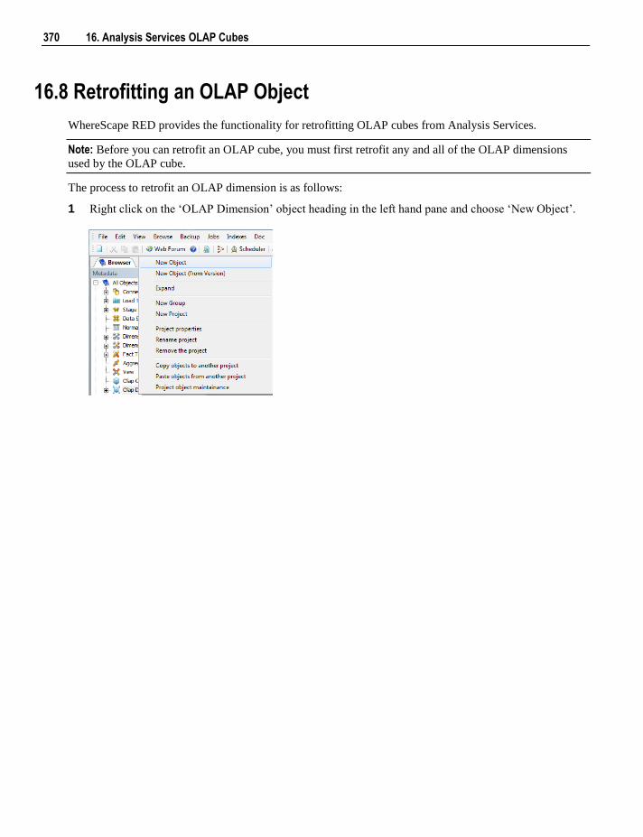
370 16. Analysis Services OLAP Cubes
16.8 Retrofitting an OLAP Object
WhereScape RED provides the functionality for retrofitting OLAP cubes from Analysis Services.
Note: Before you can retrofit an OLAP cube, you must first retrofit any and all of the OLAP dimensions
used by the OLAP cube.
The process to retrofit an OLAP dimension is as follows:
1 Right click on the „OLAP Dimension‟ object heading in the left hand pane and choose „New Object‟.
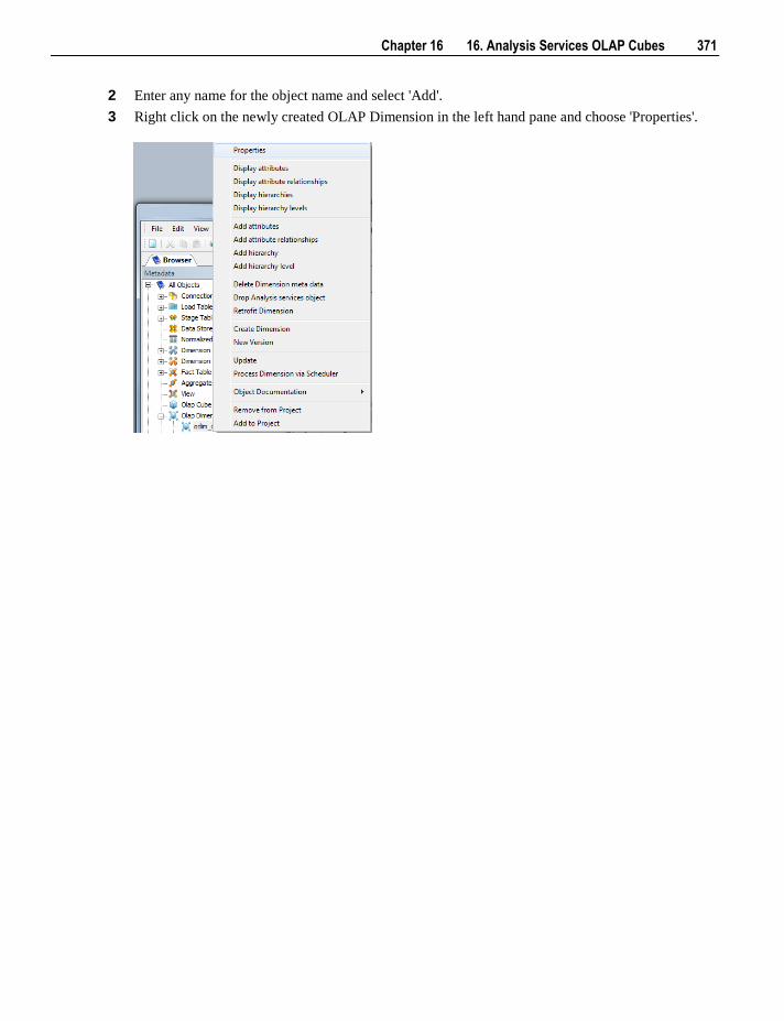
Chapter 16 16. Analysis Services OLAP Cubes 371
2 Enter any name for the object name and select 'Add'.
3 Right click on the newly created OLAP Dimension in the left hand pane and choose 'Properties'.
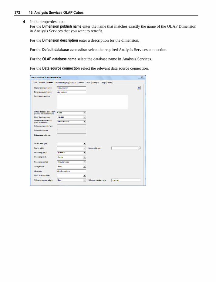
372 16. Analysis Services OLAP Cubes
4 In the properties box:
For the Dimension publish name enter the name that matches exactly the name of the OLAP Dimension
in Analysis Services that you want to retrofit.
For the Dimension description enter a description for the dimension.
For the Default database connection select the required Analysis Services connection.
For the OLAP database name select the database name in Analysis Services.
For the Data source connection select the relevant data source connection.
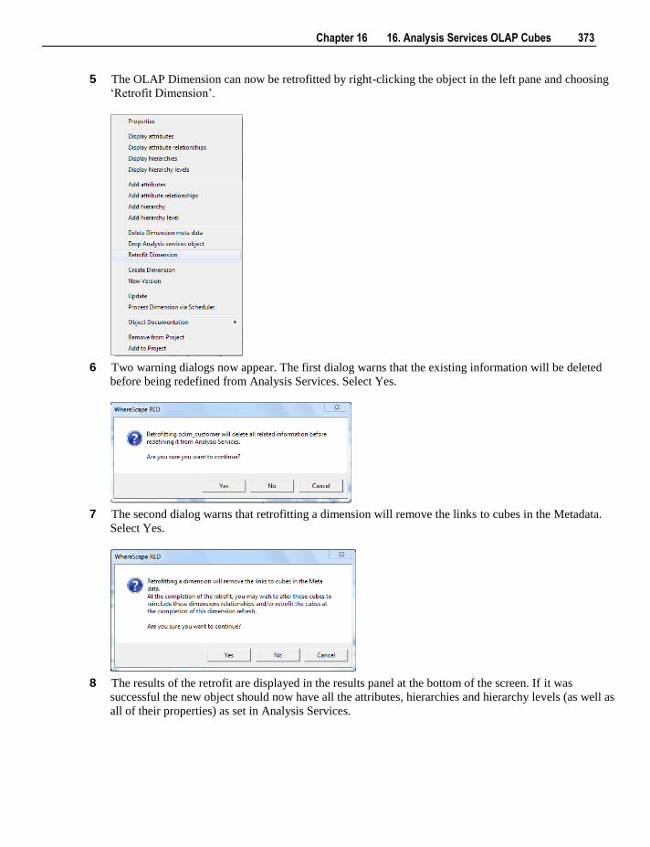
Chapter 16 16. Analysis Services OLAP Cubes 373
5 The OLAP Dimension can now be retrofitted by right-clicking the object in the left pane and choosing
„Retrofit Dimension‟.
6 Two warning dialogs now appear. The first dialog warns that the existing information will be deleted
before being redefined from Analysis Services. Select Yes.
7 The second dialog warns that retrofitting a dimension will remove the links to cubes in the Metadata.
Select Yes.
8 The results of the retrofit are displayed in the results panel at the bottom of the screen. If it was
successful the new object should now have all the attributes, hierarchies and hierarchy levels (as well as
all of their properties) as set in Analysis Services.
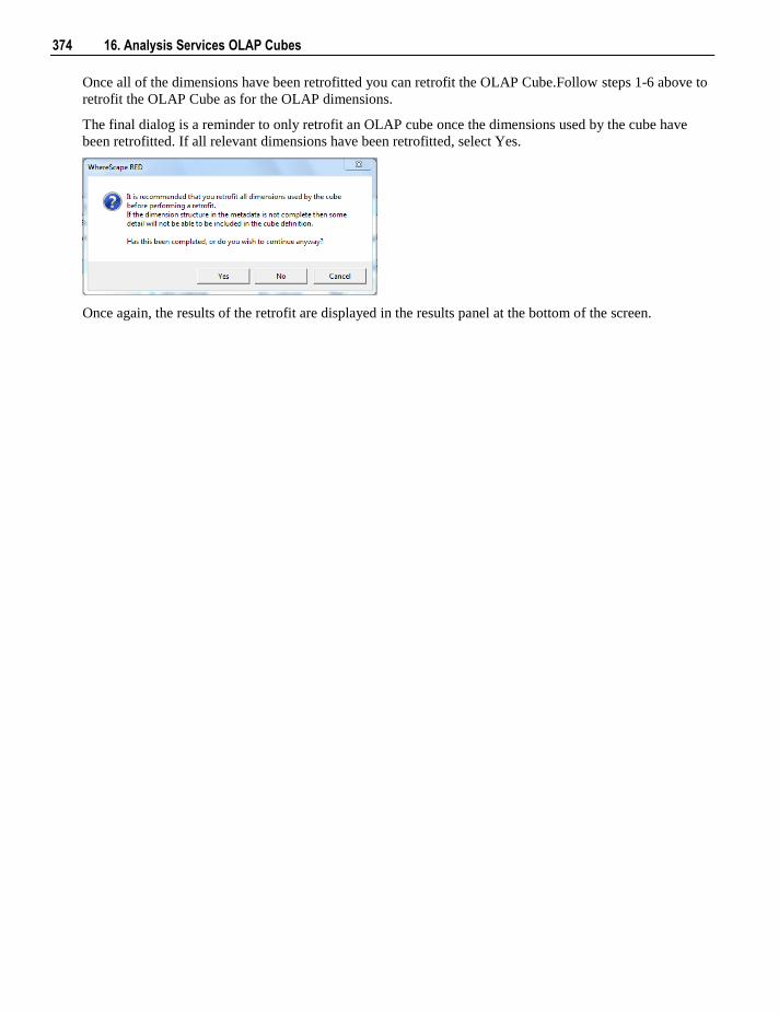
374 16. Analysis Services OLAP Cubes
Once all of the dimensions have been retrofitted you can retrofit the OLAP Cube.Follow steps 1-6 above to
retrofit the OLAP Cube as for the OLAP dimensions.
The final dialog is a reminder to only retrofit an OLAP cube once the dimensions used by the cube have
been retrofitted. If all relevant dimensions have been retrofitted, select Yes.
Once again, the results of the retrofit are displayed in the results panel at the bottom of the screen.
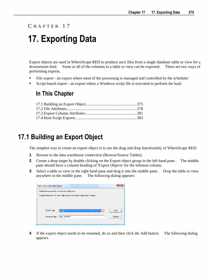
Chapter 17 17. Exporting Data 375
Export objects are used in WhereScape RED to produce ascii files from a single database table or view for a
downstream feed. Some or all of the columns in a table or view can be exported. There are two ways of
performing exports.
File export - an export where most of the processing is managed and controlled by the scheduler
Script-based export - an export where a Windows script file is executed to perform the load.
In This Chapter
17.1 Building an Export Object ................................................... 375
17.2 File Attributes ...................................................................... 378
17.3 Export Column Attributes ................................................... 381
17.4 Host Script Exports ............................................................. 383
17.1 Building an Export Object
The simplest way to create an export object is to use the drag and drop functionality of WhereScape RED.
1 Browse to the data warehouse connection (Browse/Source Tables).
2 Create a drop target by double clicking on the Export object group in the left hand pane. The middle
pane should have a column heading of 'Export Objects' for the leftmost column.
3 Select a table or view in the right hand pane and drag it into the middle pane. Drop the table or view
anywhere in the middle pane. The following dialog appears:
4 If the export object needs to be renamed, do so and then click the Add button. The following dialog
appears.
C H A P T E R 1 7
17. Exporting Data
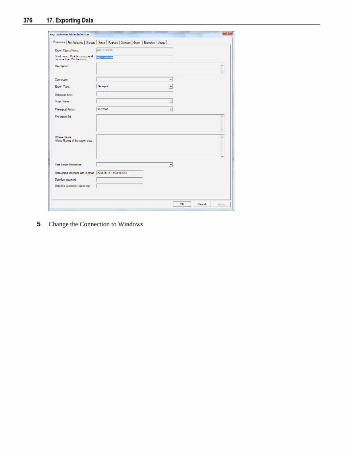
376 17. Exporting Data
5 Change the Connection to Windows
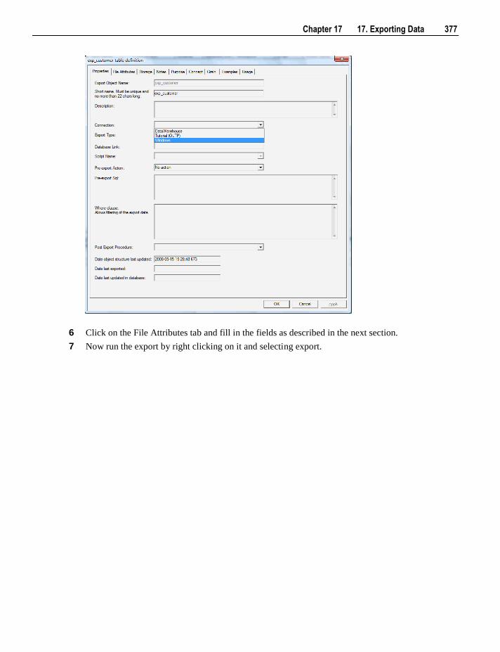
Chapter 17 17. Exporting Data 377
6 Click on the File Attributes tab and fill in the fields as described in the next section.
7 Now run the export by right clicking on it and selecting export.
378 17. Exporting Data
17.2 File Attributes
The following fields are available to define the location, name and contents of the exported data file:
Export File Path
The full path name to the directory in which the file is to be created on the Windows system.
Export File Name
The name of the file in the directory.
Export Routine
For Oracle this is SQL*Plus. In SQL Server 2000 this is BCP or isql. In later versions of SQL Server
this is BCP or sqlcmd. For DB2 the supported export routine is EXPORT.
Export Format
This is the format of the data in the export file and is either Delimited Text or Width Fixed Text in Oracle
and SQL Server. In DB2, the supported formats are DEL (delimited), WSF (worksheet format) and
IXF(intergrated exchange format).
Export File Delimiter
Any delimiter in the file that splits out the columns, e.g, a comma (,). To enter a special character enter the
uppercase string CHAR with the ASCII value in brackets (e.g. CHAR(9) ). This is only available if the
Export Format is Delimited Text.
Optionally Enclosed by
Character to enclose each text field with. This is only available if the Export Format is Delimited Text.
Header row in export file
If a header line is required, choose business names or column names from this drop down list. This option
is not available in DB2.
Export options
Allows the entry of export utility options. If more than one option is required, then a semi-colon should be
used between options. This option is not available in DB2.
Export modifier
Allows the entry of EXPORT modifiers in DB2.
Trigger Path
Chapter 17 17. Exporting Data 379
The purpose of the trigger file is to indicate that the copying / loading of the main file has completed and
that it is now safe to load the file. Secondly the trigger file may contain control sums to validate the
contents of the main load file. This field should contain the full path name to the directory in which a
trigger file is to be generated on the Windows systems.
Trigger Name
Refers to the name of the file that is to be created as a trigger file. A trigger file typically contains check
sums (row count or the sum of a numeric column).
Trigger Delimiter
Multiple fields in the trigger file are to be separated by the trigger delimiter.
Trigger Parameter 1,2,3
The checksums to be put in the trigger file. One of the row count and the sum of any numeric fields in the
source data.
Compress after export
Check this box if you want to compress the export file after it has been created.
Compress Utility Path
The directory in which the compress utility exists.
Compress Utility Name
The name of the compression utility executable.
Compress Utility Parameters
The name of the file to be compressed (using the WhereScape RED variable $EXPFILE$) and any switches
required to make the compression utility work.
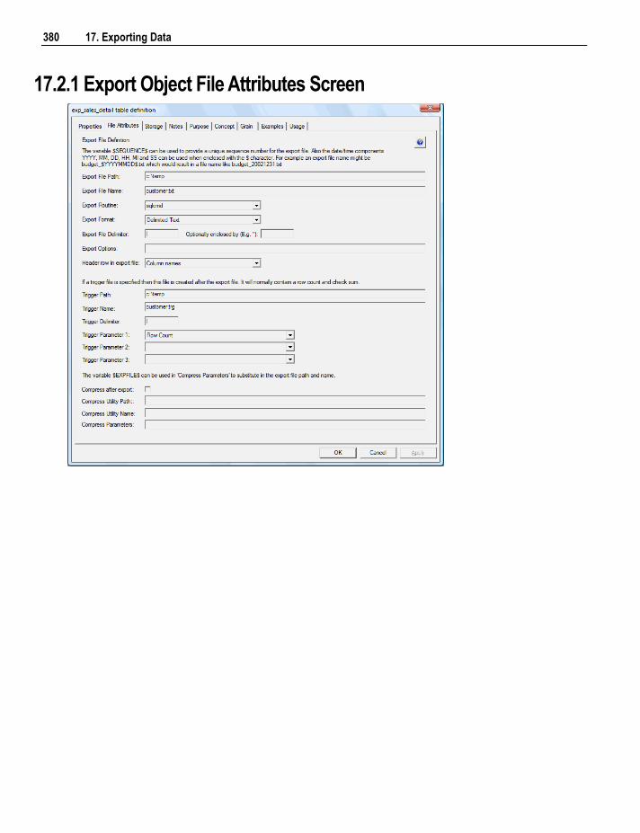
380 17. Exporting Data
17.2.1 Export Object File Attributes Screen
Chapter 17 17. Exporting Data 381
17.3 Export Column Attributes
Table
The export object to which the column belongs. Read only.
Column name
The name of the column in the export object. This name must conform to database column naming
standards. Typically such standards exclude the use of spaces etc. A good practice is to only use
alphanumerics and the underscore character. Changing this field alters the table's definition.
Business display name
This defines how the business refers to this column. It provides input to the documentation and to the view
ws_admin_v_fact_col which can be used to assist in the population of an end user tool's end user layer. As
such it is a free form entry and any characters are valid.
Data type
This is the database specific data type. It must be a valid data type for the data warehouse database
platform. The data type determines the space used by the column in a fixed width export.
Column order
This numeric field provides the ordering of the columns in the database table create statement. The lowest
numbered column will appear first in the table. Although this affects the physical table definition no action
will be taken unless the table is re-created in the database. The columns can be re-numbered based on the
existing order by choosing the 'Respace order number' pop-up menu option when positioned over any
column in the table. This action will number the columns in increments of 10 starting at 10. In addition to
a simple change of the order field, the column order can be changed by first displaying the columns in the
middle pane and then using drag and drop to move the columns around. This drag and drop process will
automatically renumber the columns as required.
Format
Not relevant for Export Objects.
Nulls
Not relevant for Export Objects.
Numeric
Not relevant for Export Objects.
Additive
Not relevant for Export Objects.
Attribute
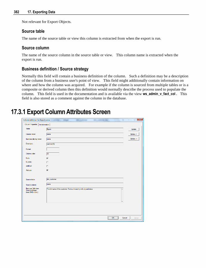
382 17. Exporting Data
Not relevant for Export Objects.
Source table
The name of the source table or view this column is extracted from when the export is run.
Source column
The name of the source column in the source table or view. This column name is extracted when the
export is run.
Business definition / Source strategy
Normally this field will contain a business definition of the column. Such a definition may be a description
of the column from a business user's point of view. This field might additionally contain information on
where and how the column was acquired. For example if the column is sourced from multiple tables or is a
composite or derived column then this definition would normally describe the process used to populate the
column. This field is used in the documentation and is available via the view ws_admin_v_fact_col . This
field is also stored as a comment against the column in the database.
17.3.1 Export Column Attributes Screen
Chapter 17 17. Exporting Data 383
17.4 Host Script Exports
A script based export object will have a Host Script defined. During the export process this host script is
executed and the results returned.
During the 'drag and drop' creation of a export object from a single table or view, a script can be generated
by selecting one of the 'Script based' export options. This script can then be edited to more fully meet any
requirements.
There are a number of conventions that must be followed if these host scripts are to be used by the
WhereScape scheduler.
1 The first line of data in 'standard out' must contain the resultant status of the script. Valid values are '1'
to indicate success, '-1' to indicate a Warning condition occurred but the result is considered a success,
'-2' to indicate a handled Error occurred and subsequent dependent tasks should be held, -3 to indicate
an unhandled Failure and that subsequent dependent tasks should be held.
2 The second line of data in 'standard out' must contain a resultant message of no more than 256
characters.
3 Any subsequent lines in 'standard out' are considered informational and are recorded in the audit trail.
The normal practice is to place a minimum of information in the audit trail. All bulk information
should be output to 'standard error'
4 Any data output to 'standard error' will be written to the error/detail log. Both the audit log and detail
log can be viewed from the WhereScape RED tool under the scheduler window.

Chapter 18 18. MicroStrategy Projects 385
MicroStrategy Projects can be designed and created from within the WhereScape RED framework. This
chapter covers the procedures required to create and manage these MicroStrategy Projects.
In This Chapter
18.1 MicroStrategy Prerequisites ................................................ 385
18.2 Building MicroStrategy Projects ......................................... 385
18.1 MicroStrategy Prerequisites
Before building MicroStrategy projects using WhereScape RED, the following prerequisites are required:
MicroStrategy must be installed on the Developer's PC.
Install the WhereScape RED for MicroStratgey extension package. This is a separately shipped
package that you must acquire via your account or partner manager.
Note: Installing this package enables the Tools/Build MicroStrategy Project menu in WhereScape RED.
18.2 Building MicroStrategy Projects
For full instructions for build MicroStrategy Projects, refer to the documentation contained in the
WhereScape RED for MicroStratgey extension package.
C H A P T E R 1 8
18. MicroStrategy Projects

Chapter 19 19. Transformations 387
Standard column transformations (see "19.1 Column Transformations" on page 387) can be used in
WhereScape RED to perform calculations, change data types or format data.
Re-using complex transformations can save a significant amount of time. These can be achieved in two
ways with WhereScape RED:
Database Functions
WhereScape RED Re-usable Transformations
In This Chapter
19.1 Column Transformations .................................................... 387
19.2 Database Functions ............................................................. 393
19.3 Re-usable Transformations ................................................. 393
19.1 Column Transformations
Each table or export object column can have a transformation associated with it. For all table types, except
for load tables, the transformation will be included in the generated procedure for the table. These are
executed as part of the procedure update. The transformation must therefore be a valid SQL construct that
can be included in a 'Select' statement. For example, we could have a transformation of
'load_order_line.qty * 0.125' to calculate a tax column of 12.5%. Click the 'Transformation' tab on the
column properties to enter a transformation.
Note: Transformations added to an existing table that have an update procedure are only put into effect
when the procedure is re-generated and re-compiled.
Column transformations on load tables are more complex, due to the unique nature of load tables. See
Load Table Column Transformations (see "19.1.2 Load Table Column Transformations" on page 390)
for more details.
Dimension View transformations are included in the Database Definition Language (DDL) that creates the
view in the database. Any changes to Dimension View column transformations require the view to be
dropped and recreated.
Export object column transformations are dynamically applied for file exports. If the export object is
executed via a host script, then the script needs to be regenerated for changes to transformations to take
effect.
C H A P T E R 1 9
19. Transformations
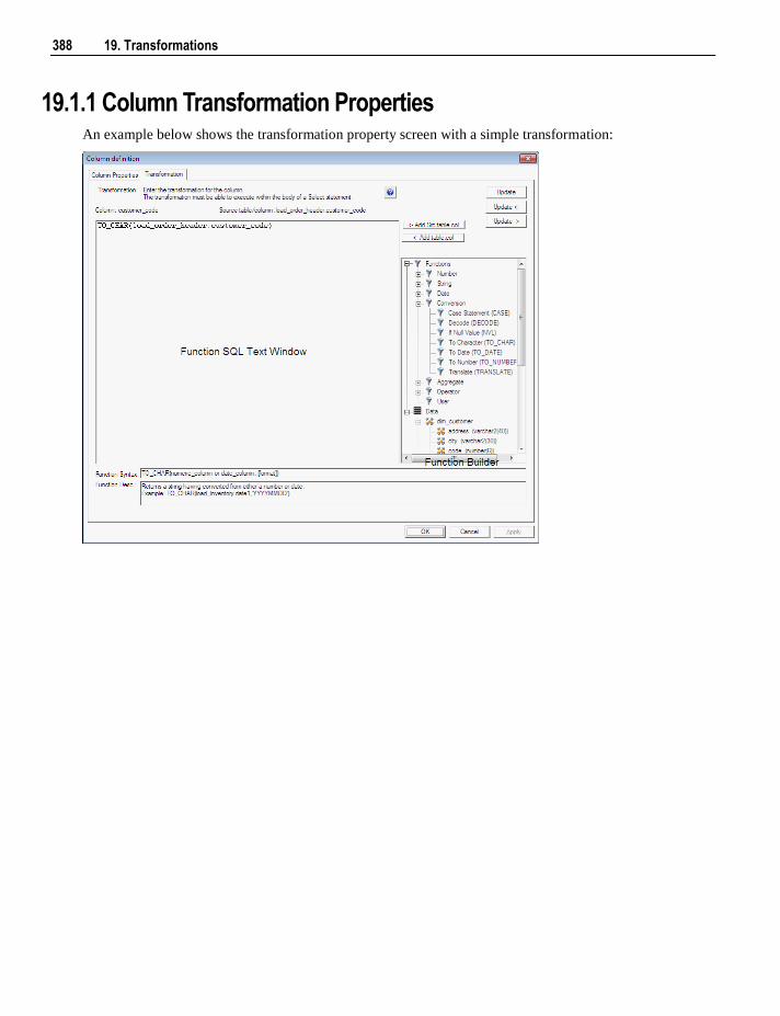
388 19. Transformations
19.1.1 Column Transformation Properties An example below shows the transformation property screen with a simple transformation:
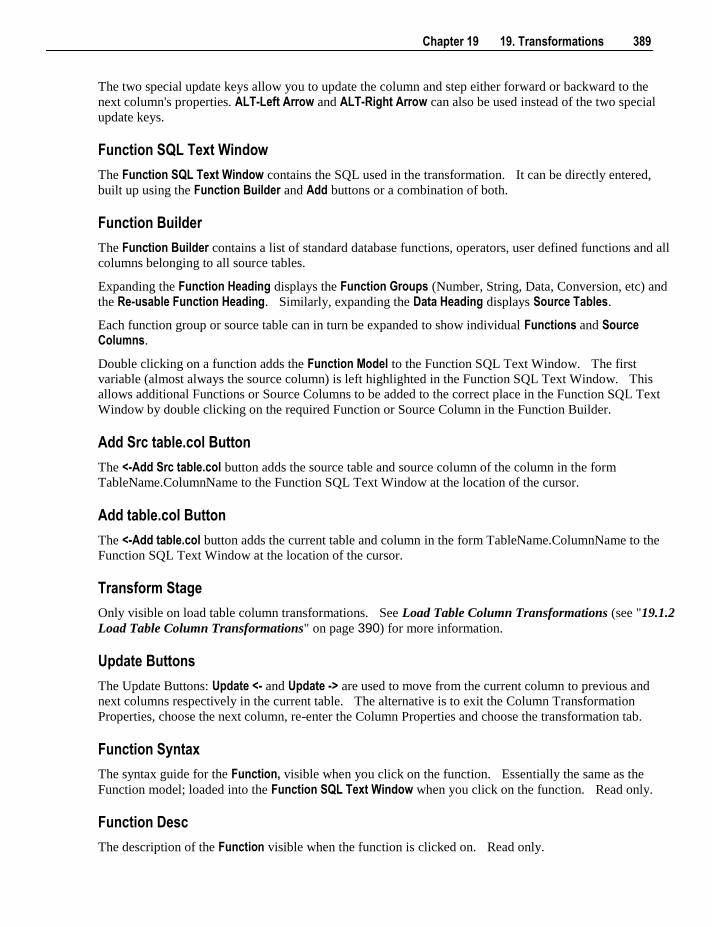
Chapter 19 19. Transformations 389
The two special update keys allow you to update the column and step either forward or backward to the
next column's properties. ALT-Left Arrow and ALT-Right Arrow can also be used instead of the two special
update keys.
Function SQL Text Window
The Function SQL Text Window contains the SQL used in the transformation. It can be directly entered,
built up using the Function Builder and Add buttons or a combination of both.
Function Builder
The Function Builder contains a list of standard database functions, operators, user defined functions and all
columns belonging to all source tables.
Expanding the Function Heading displays the Function Groups (Number, String, Data, Conversion, etc) and
the Re-usable Function Heading. Similarly, expanding the Data Heading displays Source Tables.
Each function group or source table can in turn be expanded to show individual Functions and Source Columns.
Double clicking on a function adds the Function Model to the Function SQL Text Window. The first
variable (almost always the source column) is left highlighted in the Function SQL Text Window. This
allows additional Functions or Source Columns to be added to the correct place in the Function SQL Text
Window by double clicking on the required Function or Source Column in the Function Builder.
Add Src table.col Button
The <-Add Src table.col button adds the source table and source column of the column in the form
TableName.ColumnName to the Function SQL Text Window at the location of the cursor.
Add table.col Button
The <-Add table.col button adds the current table and column in the form TableName.ColumnName to the
Function SQL Text Window at the location of the cursor.
Transform Stage
Only visible on load table column transformations. See Load Table Column Transformations (see "19.1.2
Load Table Column Transformations" on page 390) for more information.
Update Buttons
The Update Buttons: Update <- and Update -> are used to move from the current column to previous and
next columns respectively in the current table. The alternative is to exit the Column Transformation
Properties, choose the next column, re-enter the Column Properties and choose the transformation tab.
Function Syntax
The syntax guide for the Function, visible when you click on the function. Essentially the same as the
Function model; loaded into the Function SQL Text Window when you click on the function. Read only.
Function Desc
The description of the Function visible when the function is clicked on. Read only.
390 19. Transformations
Function Model
The model (template SQL code) for a Re-usable Transformations. This is only visible for Re-usable
Transformations. Read only.
Localize Transformation
The Localize transformation button breaks the link between a column transformation and the Re-usable Transformation it is based on. If this button is clicked on, changes to the underlying re-usable
transformation cannot be automatically propagated to the column transformation. This is only visible for
Re-usable Transformations.
19.1.2 Load Table Column Transformations
Overview
Data entering the data warehouse can be manipulated if required. This manipulation can occur at any
stage, but is supported via a number of methods during the Load stage. Load tables provide options to
transform data. If multiple pass transformations are required then a load table can be created from another
load table, i.e. multiple load tables can be supported in the data flow path.
The options available differ depending on the type of load but in most cases the "after" transformation and
post load procedure can be utilized. Specifically:
Database Link Load During Load transformations
After Load transformations
Post Load procedure
ODBC Based Load During Load transformations
After Load transformations
Post load procedure
File Based Load During Load transformations
After Load transformations
Post load procedure
Script Based Load During Load transformations
After Load transformations
Post load procedure
Externally Loaded After Load transformations
Post Load procedure
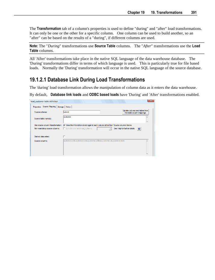
Chapter 19 19. Transformations 391
The Transformation tab of a column's properties is used to define "during" and "after" load transformations.
It can only be one or the other for a specific column. One column can be used to build another, so an
"after" can be based on the results of a "during", if different columns are used.
Note: The "During" transformations use Source Table columns. The "After" transformations use the Load Table columns.
All 'After' transformations take place in the native SQL language of the data warehouse database. The
'During' transformations differ in terms of which language is used. This is particularly true for file based
loads. Normally the 'During' transformation will occur in the native SQL language of the source database.
19.1.2.1 Database Link During Load Transformations
The 'during' load transformation allows the manipulation of column data as it enters the data warehouse.
By default, Database link loads and ODBC based loads have 'During' and 'After' transformations enabled.
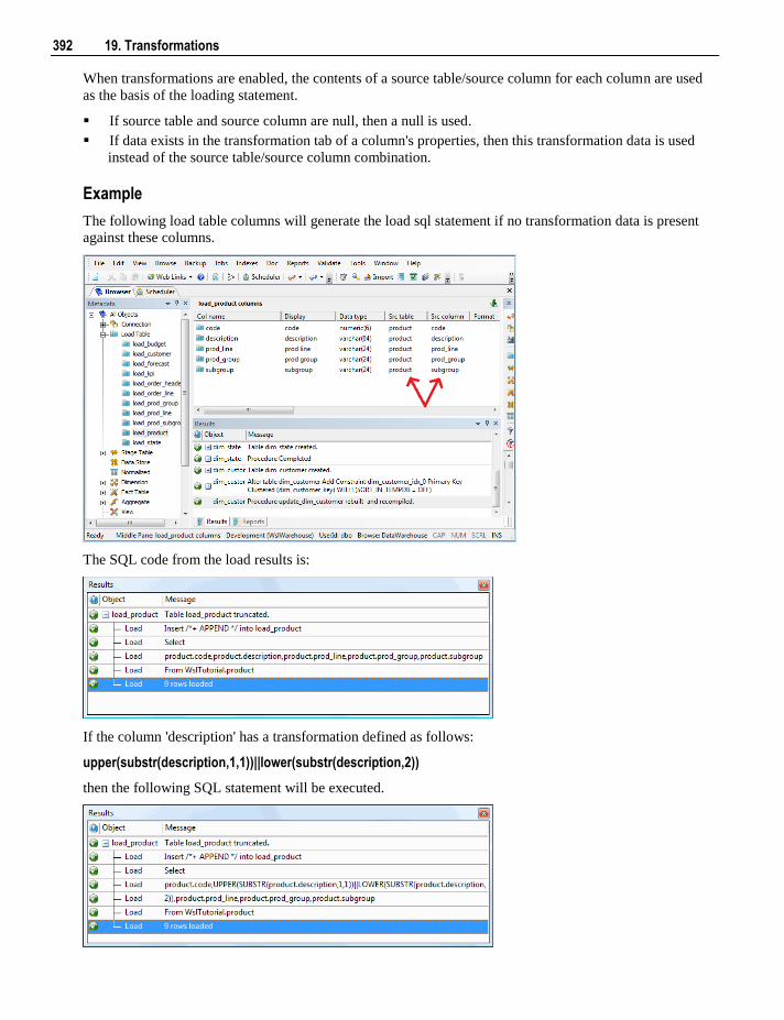
392 19. Transformations
When transformations are enabled, the contents of a source table/source column for each column are used
as the basis of the loading statement.
If source table and source column are null, then a null is used.
If data exists in the transformation tab of a column's properties, then this transformation data is used
instead of the source table/source column combination.
Example
The following load table columns will generate the load sql statement if no transformation data is present
against these columns.
The SQL code from the load results is:
If the column 'description' has a transformation defined as follows:
upper(substr(description,1,1))||lower(substr(description,2))
then the following SQL statement will be executed.
Chapter 19 19. Transformations 393
19.1.2.2 File During Load Transformations
The loading of flat files is performed using the database specific loader. For Oracle, this is
SQL*LOADER. For SQL Server it is the Bulk Insert Transact SQL statement. The contents of the
transformation tab in the column's properties are the functions and conversions supported by the database
loader.
Example
SQL*LOADER performs transformations such as:
DATE 'DD-MMM-YYYY' converts from a value such as 23-Mar-1999 to an Oracle date.
"TO_NUMBER(:COL)" converts the data to a number
"NVL(TRIM(:COL),0)" trims leading and trailing white characters and inserts zero if null.
19.1.2.3 After Load Transformations
'After' transformations will initiate a pass of the load table after the load has occurred. They allow
manipulation of the load table columns using the database and SQL functions.
Example
The following 'after' transformation set for the column code in the table load_product
lpad(code,5,'0')
would result in the following SQL statement being executed after the load:
update load_product set code = lpad(code,5,'0');
19.2 Database Functions
Database functions can be created in the data warehouse database (as procedure objects in WhereScape
RED) and used in column transformation in WhereScape RED. See the Oracle and SQL Server
documentation on functions and Procedures and Scripts (see "20. Procedures and Scripts" on page 401)
for more information on creating functions inside WhereScape RED.
19.3 Re-usable Transformations
WhereScape RED Re-usable Transformations allow a complex SQL transformation using standard database
functions (including User Defined Functions) to be built once and reused in multiple column
transformations. Functionality is included to manage and propagate changes to re-usable transformations.
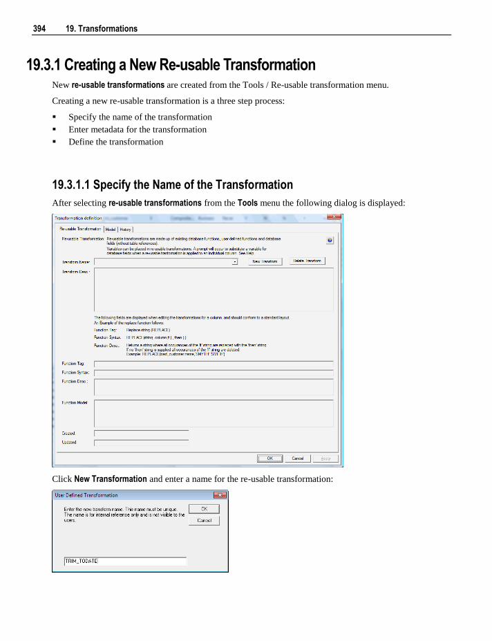
394 19. Transformations
19.3.1 Creating a New Re-usable Transformation New re-usable transformations are created from the Tools / Re-usable transformation menu.
Creating a new re-usable transformation is a three step process:
Specify the name of the transformation
Enter metadata for the transformation
Define the transformation
19.3.1.1 Specify the Name of the Transformation
After selecting re-usable transformations from the Tools menu the following dialog is displayed:
Click New Transformation and enter a name for the re-usable transformation:
Chapter 19 19. Transformations 395
Note: This is the internal WhereScape RED name for the transformation, not the name developers reference
when utilizing the transformation on column transformations.
Click OK.
19.3.1.2 Enter Re-usable Transformation Metadata
Enter the following metadata for the transformation to describe the transformation for developers.
Transform Desc
A general description of the transformation.
Function Tag
This is the function name visible to the users, which can be selected from the function builder when
building column transformations.
Function Syntax
The syntax guide for the function. This is visible in the function builder when clicking on the User defined
function.
Function Desc
The description of the function visible in the function builder when clicking on the User defined function.
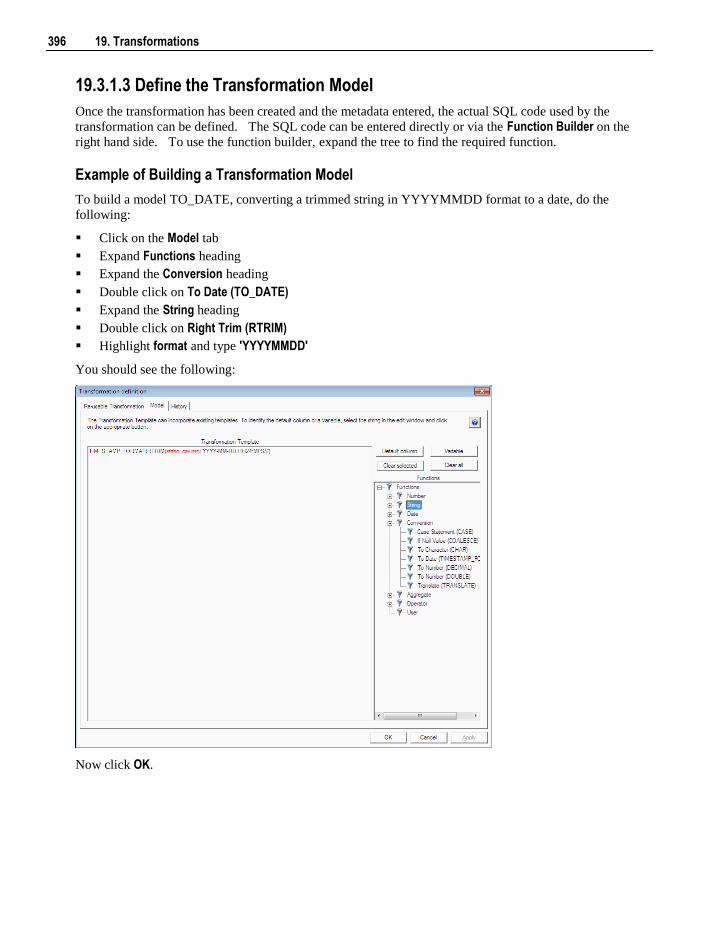
396 19. Transformations
19.3.1.3 Define the Transformation Model
Once the transformation has been created and the metadata entered, the actual SQL code used by the
transformation can be defined. The SQL code can be entered directly or via the Function Builder on the
right hand side. To use the function builder, expand the tree to find the required function.
Example of Building a Transformation Model
To build a model TO_DATE, converting a trimmed string in YYYYMMDD format to a date, do the
following:
Click on the Model tab
Expand Functions heading
Expand the Conversion heading
Double click on To Date (TO_DATE)
Expand the String heading
Double click on Right Trim (RTRIM)
Highlight format and type 'YYYYMMDD'
You should see the following:
Now click OK.
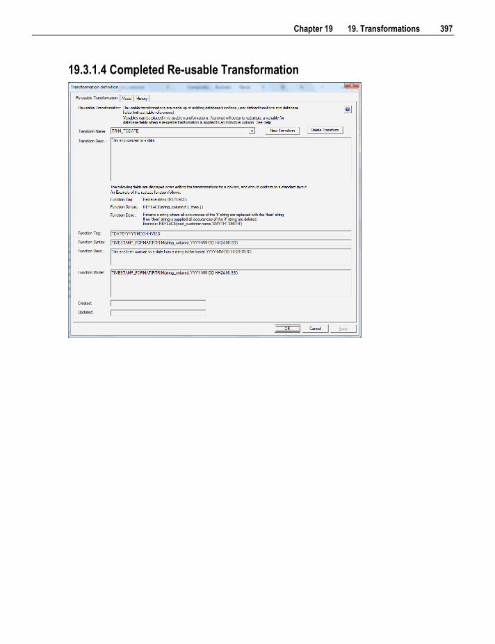
Chapter 19 19. Transformations 397
19.3.1.4 Completed Re-usable Transformation
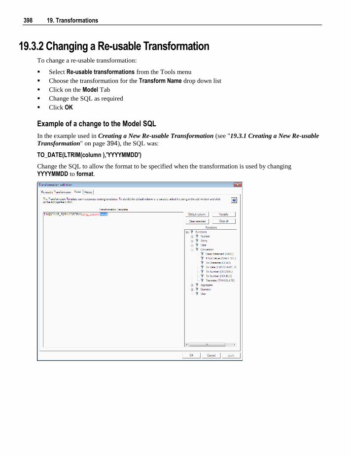
398 19. Transformations
19.3.2 Changing a Re-usable Transformation To change a re-usable transformation:
Select Re-usable transformations from the Tools menu
Choose the transformation for the Transform Name drop down list
Click on the Model Tab
Change the SQL as required
Click OK
Example of a change to the Model SQL
In the example used in Creating a New Re-usable Transformation (see "19.3.1 Creating a New Re-usable
Transformation" on page 394), the SQL was:
TO_DATE(LTRIM(column ),'YYYYMMDD')
Change the SQL to allow the format to be specified when the transformation is used by changing
YYYYMMDD to format.
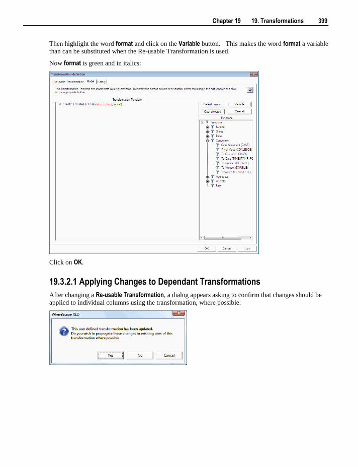
Chapter 19 19. Transformations 399
Then highlight the word format and click on the Variable button. This makes the word format a variable
than can be substituted when the Re-usable Transformation is used.
Now format is green and in italics:
Click on OK.
19.3.2.1 Applying Changes to Dependant Transformations
After changing a Re-usable Transformation, a dialog appears asking to confirm that changes should be
applied to individual columns using the transformation, where possible:
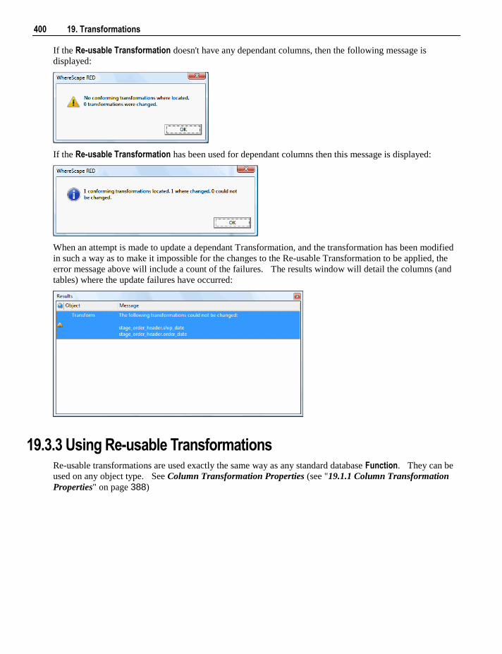
400 19. Transformations
If the Re-usable Transformation doesn't have any dependant columns, then the following message is
displayed:
If the Re-usable Transformation has been used for dependant columns then this message is displayed:
When an attempt is made to update a dependant Transformation, and the transformation has been modified
in such a way as to make it impossible for the changes to the Re-usable Transformation to be applied, the
error message above will include a count of the failures. The results window will detail the columns (and
tables) where the update failures have occurred:
19.3.3 Using Re-usable Transformations Re-usable transformations are used exactly the same way as any standard database Function. They can be
used on any object type. See Column Transformation Properties (see "19.1.1 Column Transformation
Properties" on page 388)
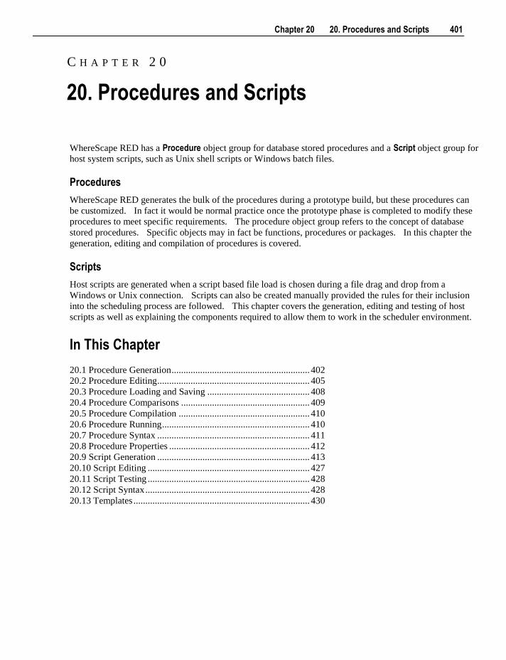
Chapter 20 20. Procedures and Scripts 401
WhereScape RED has a Procedure object group for database stored procedures and a Script object group for
host system scripts, such as Unix shell scripts or Windows batch files.
Procedures
WhereScape RED generates the bulk of the procedures during a prototype build, but these procedures can
be customized. In fact it would be normal practice once the prototype phase is completed to modify these
procedures to meet specific requirements. The procedure object group refers to the concept of database
stored procedures. Specific objects may in fact be functions, procedures or packages. In this chapter the
generation, editing and compilation of procedures is covered.
Scripts
Host scripts are generated when a script based file load is chosen during a file drag and drop from a
Windows or Unix connection. Scripts can also be created manually provided the rules for their inclusion
into the scheduling process are followed. This chapter covers the generation, editing and testing of host
scripts as well as explaining the components required to allow them to work in the scheduler environment.
In This Chapter
20.1 Procedure Generation .......................................................... 402
20.2 Procedure Editing ................................................................ 405
20.3 Procedure Loading and Saving ........................................... 408
20.4 Procedure Comparisons ...................................................... 409
20.5 Procedure Compilation ....................................................... 410
20.6 Procedure Running .............................................................. 410
20.7 Procedure Syntax ................................................................ 411
20.8 Procedure Properties ........................................................... 412
20.9 Script Generation ................................................................ 413
20.10 Script Editing .................................................................... 427
20.11 Script Testing .................................................................... 428
20.12 Script Syntax ..................................................................... 428
20.13 Templates .......................................................................... 430
C H A P T E R 2 0
20. Procedures and Scripts
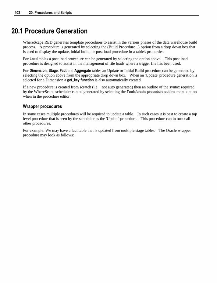
402 20. Procedures and Scripts
20.1 Procedure Generation
WhereScape RED generates template procedures to assist in the various phases of the data warehouse build
process. A procedure is generated by selecting the (Build Procedure...) option from a drop down box that
is used to display the update, initial build, or post load procedure in a table's properties.
For Load tables a post load procedure can be generated by selecting the option above. This post load
procedure is designed to assist in the management of file loads where a trigger file has been used.
For Dimension, Stage, Fact and Aggregate tables an Update or Initial Build procedure can be generated by
selecting the option above from the appropriate drop down box. When an 'Update' procedure generation is
selected for a Dimension a get_key function is also automatically created.
If a new procedure is created from scratch (i.e. not auto generated) then an outline of the syntax required
by the WhereScape scheduler can be generated by selecting the Tools/create procedure outline menu option
when in the procedure editor.
Wrapper procedures
In some cases multiple procedures will be required to update a table. In such cases it is best to create a top
level procedure that is seen by the scheduler as the 'Update' procedure. This procedure can in turn call
other procedures.
For example: We may have a fact table that is updated from multiple stage tables. The Oracle wrapper
procedure may look as follows:
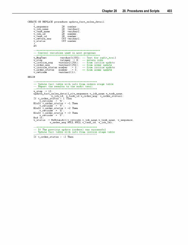
Chapter 20 20. Procedures and Scripts 403
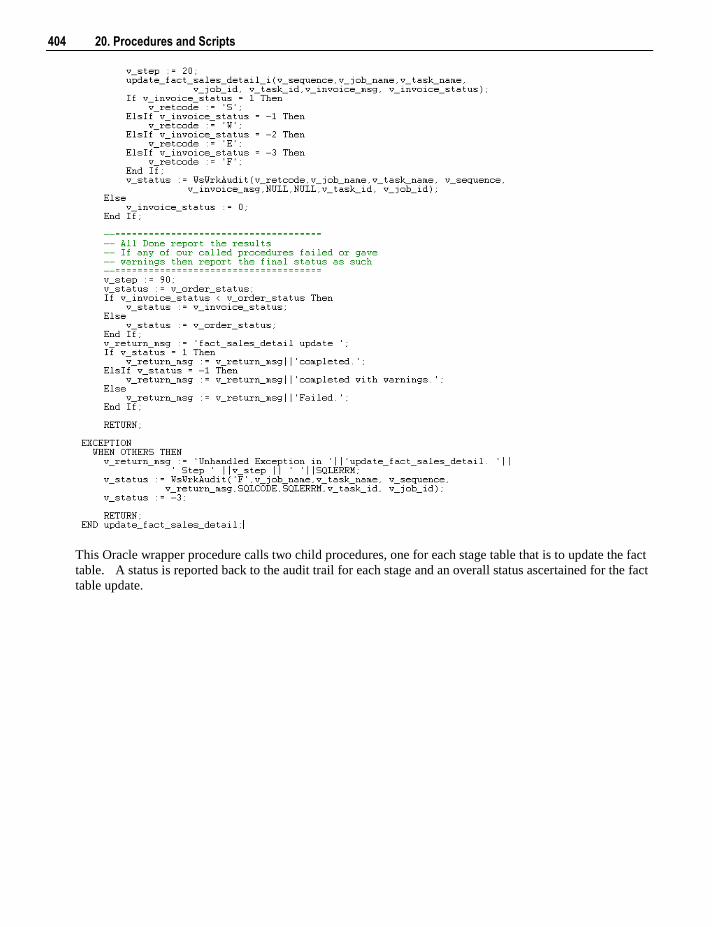
404 20. Procedures and Scripts
This Oracle wrapper procedure calls two child procedures, one for each stage table that is to update the fact
table. A status is reported back to the audit trail for each stage and an overall status ascertained for the fact
table update.
Chapter 20 20. Procedures and Scripts 405
20.2 Procedure Editing
WhereScape RED includes a procedure editor which allows the maintenance of the various procedures,
functions and packages within the data warehouse. The editor is invoked by double clicking on a
procedure name in the left hand pane or by selecting the 'Edit the procedure' pop-up menu option when a
right mouse menu is activated on the procedure name.
A procedure can be compiled by selecting the Compile/Compile menu option. See the section on
compiling procedures for more information.
This section will discuss some of the features of the procedure editor.
In the following sections reference is made to a selected block of text. A selected block of text is a normal
windows selection where the text in question is highlighted. Normally achieved by holding down the left
mouse button and moving the cursor.
Indenting code
The tab character inserts four spaces into the text. A shift/tab removes four spaces.
Cut, Copy, Paste and Delete
The normal Windows cut, copy, paste and delete functions are available either through the toolbar or via the
right mouse popup menu.
Indenting a block of text
A selected block of text can be indented by four spaces by depressing the tab character. Each tab will
indent by a further four spaces. A shift/tab will remove four spaces from the front of each line in the
selected block.
Commenting out a block of text
A selected block of text can be turned into a comment by using the 'Comment' option in the right mouse
pop-up menu. The editor will place two dashes '--' at the front of each line in the selected block. In the
same way a block of text can be uncommented by choosing the 'UnComment' option. Note that only lines
that start with two dashes in the left most column can be uncommented.
Inserting Steps
The right mouse pop-up menu has an option to insert step. This option will insert a code line of the format
'v_step := 1000;'. Each subsequent insert will add 100 to the step value. The Alt/Z key can also be used to
insert a step line.
The v_step variable is used in the event of an unhandled exception. In such a case the current v_step value
is reported, and it may be possible to ascertain the code that failed based on the value of this v_step
variable.
Note: If a step is inserted via this method then the step numbering will be automatically reset for all steps
numbering from 100 in increments of 100 when the procedure is compiled or saved.
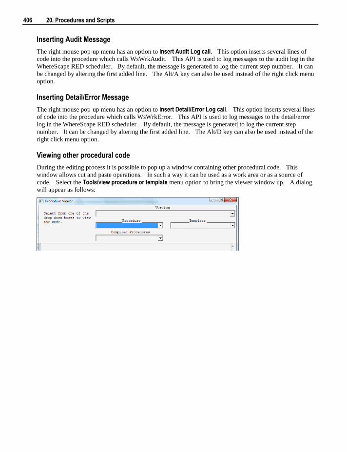
406 20. Procedures and Scripts
Inserting Audit Message
The right mouse pop-up menu has an option to Insert Audit Log call. This option inserts several lines of
code into the procedure which calls WsWrkAudit. This API is used to log messages to the audit log in the
WhereScape RED scheduler. By default, the message is generated to log the current step number. It can
be changed by altering the first added line. The Alt/A key can also be used instead of the right click menu
option.
Inserting Detail/Error Message
The right mouse pop-up menu has an option to Insert Detail/Error Log call. This option inserts several lines
of code into the procedure which calls WsWrkError. This API is used to log messages to the detail/error
log in the WhereScape RED scheduler. By default, the message is generated to log the current step
number. It can be changed by altering the first added line. The Alt/D key can also be used instead of the
right click menu option.
Viewing other procedural code
During the editing process it is possible to pop up a window containing other procedural code. This
window allows cut and paste operations. In such a way it can be used as a work area or as a source of
code. Select the Tools/view procedure or template menu option to bring the viewer window up. A dialog
will appear as follows:
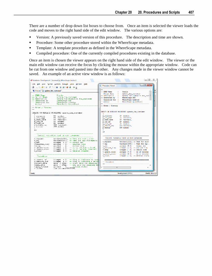
Chapter 20 20. Procedures and Scripts 407
There are a number of drop down list boxes to choose from. Once an item is selected the viewer loads the
code and moves to the right hand side of the edit window. The various options are:
Version: A previously saved version of this procedure. The description and time are shown.
Procedure: Some other procedure stored within the WhereScape metadata.
Template: A template procedure as defined in the WhereScape metadata.
Compiled procedure: One of the currently compiled procedures existing in the database.
Once an item is chosen the viewer appears on the right hand side of the edit window. The viewer or the
main edit window can receive the focus by clicking the mouse within the appropriate window. Code can
be cut from one window and pasted into the other. Any changes made in the viewer window cannot be
saved. An example of an active view window is as follows:
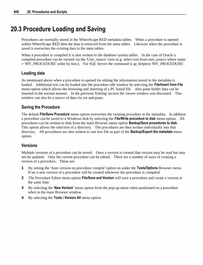
408 20. Procedures and Scripts
20.3 Procedure Loading and Saving
Procedures are normally stored in the WhereScape RED metadata tables. When a procedure is opened
within WhereScape RED then the data is retrieved from the meta tables. Likewise when the procedure is
saved it overwrites the existing data in the meta tables.
When a procedure is compiled it is also written to the database system tables. In the case of Oracle a
compiled procedure can be viewed via the 'User_source' view (e.g. select text from user_source where name
= 'MY_PROCEDURE' order by line;). For SQL Server the command is sp_helptext 'MY_PROCEDURE'.
Loading data
As mentioned above when a procedure is opened for editing the information stored in the metadata is
loaded. Additional text can be loaded into the procedure edit window by selecting the File/Insert from File
menu option which allows the browsing and inserting of a PC based file. Also paste buffer data can be
inserted in the normal manner. In the previous 'Editing' section the viewer window was discussed. This
window can also be a source of data via cut and paste.
Saving the Procedure
The default File/Save Procedure menu option overwrites the existing procedure in the metadata. In addition
a procedure can be saved to a Windows disk by selecting the File/Write procedure to disk menu option. All
procedures can be written to disk from the main Browser menu option Backup/Save procedures to disk.
This option allows the selection of a directory. The procedures are then written individually into that
directory. All procedures are also written to one text file as part of the Backup/Export the metadata menu
option.
Versions
Multiple versions of a procedure can be stored. Once a version is created that version may be read but may
not be updated. Only the current procedure can be edited. There are a number of ways of creating a
version of a procedure. These are:
1 By setting the 'Auto version on procedure compile' option on under the Tools/Options Browser menu.
If set a new version of a procedure will be created whenever the procedure is compiled.
2 The Procedure Editor menu option File/Save and Version will save a procedure and create a version at
the same time.
3 By selecting the 'New Version' menu option from the pop-up menu when positioned on a procedure
when in the main Browser window.
4 By selecting the Tools / Version All menu option.
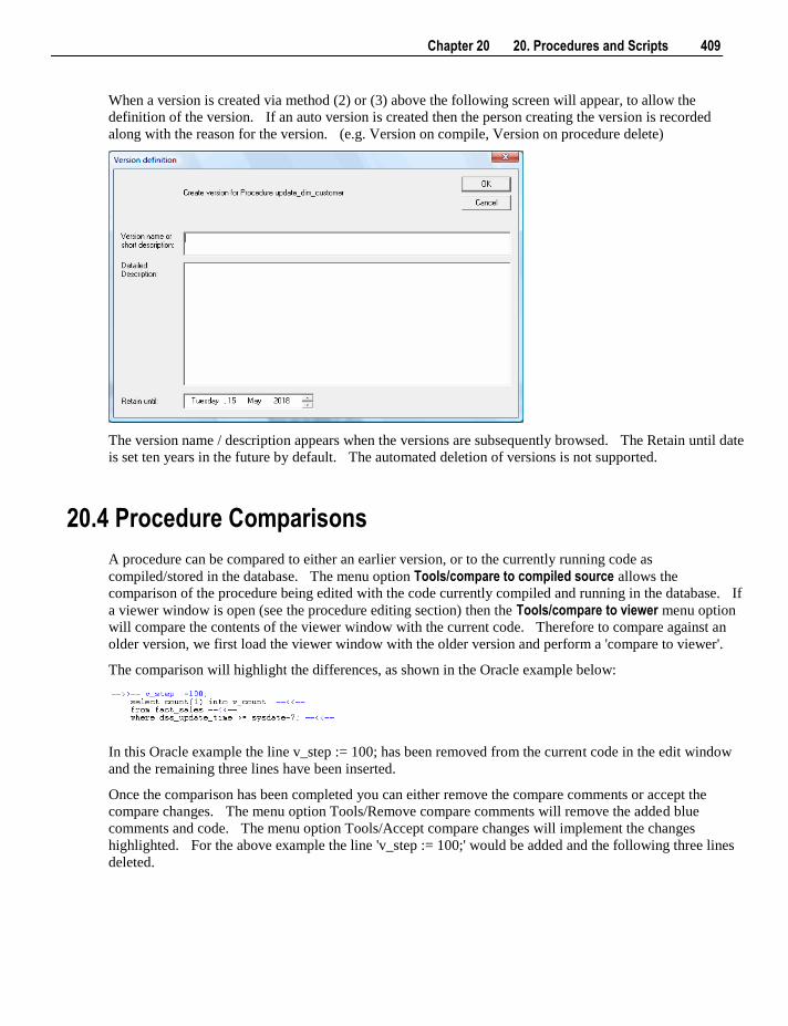
Chapter 20 20. Procedures and Scripts 409
When a version is created via method (2) or (3) above the following screen will appear, to allow the
definition of the version. If an auto version is created then the person creating the version is recorded
along with the reason for the version. (e.g. Version on compile, Version on procedure delete)
The version name / description appears when the versions are subsequently browsed. The Retain until date
is set ten years in the future by default. The automated deletion of versions is not supported.
20.4 Procedure Comparisons
A procedure can be compared to either an earlier version, or to the currently running code as
compiled/stored in the database. The menu option Tools/compare to compiled source allows the
comparison of the procedure being edited with the code currently compiled and running in the database. If
a viewer window is open (see the procedure editing section) then the Tools/compare to viewer menu option
will compare the contents of the viewer window with the current code. Therefore to compare against an
older version, we first load the viewer window with the older version and perform a 'compare to viewer'.
The comparison will highlight the differences, as shown in the Oracle example below:
In this Oracle example the line v_step := 100; has been removed from the current code in the edit window
and the remaining three lines have been inserted.
Once the comparison has been completed you can either remove the compare comments or accept the
compare changes. The menu option Tools/Remove compare comments will remove the added blue
comments and code. The menu option Tools/Accept compare changes will implement the changes
highlighted. For the above example the line 'v_step := 100;' would be added and the following three lines
deleted.
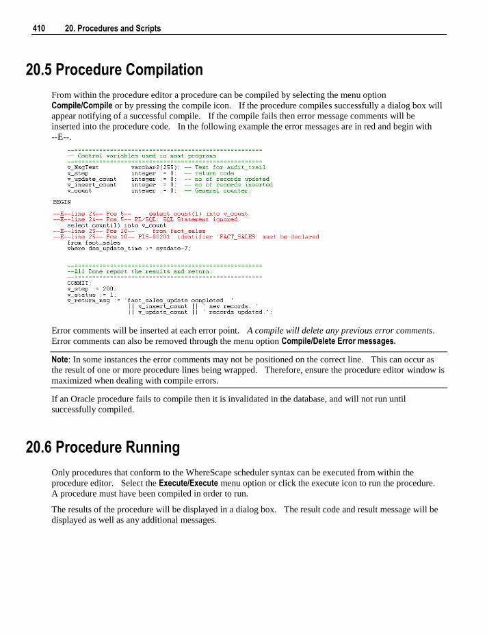
410 20. Procedures and Scripts
20.5 Procedure Compilation
From within the procedure editor a procedure can be compiled by selecting the menu option
Compile/Compile or by pressing the compile icon. If the procedure compiles successfully a dialog box will
appear notifying of a successful compile. If the compile fails then error message comments will be
inserted into the procedure code. In the following example the error messages are in red and begin with
--E--.
Error comments will be inserted at each error point. A compile will delete any previous error comments.
Error comments can also be removed through the menu option Compile/Delete Error messages.
Note: In some instances the error comments may not be positioned on the correct line. This can occur as
the result of one or more procedure lines being wrapped. Therefore, ensure the procedure editor window is
maximized when dealing with compile errors.
If an Oracle procedure fails to compile then it is invalidated in the database, and will not run until
successfully compiled.
20.6 Procedure Running
Only procedures that conform to the WhereScape scheduler syntax can be executed from within the
procedure editor. Select the Execute/Execute menu option or click the execute icon to run the procedure.
A procedure must have been compiled in order to run.
The results of the procedure will be displayed in a dialog box. The result code and result message will be
displayed as well as any additional messages.
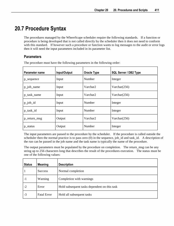
Chapter 20 20. Procedures and Scripts 411
20.7 Procedure Syntax
The procedures managed by the WhereScape scheduler require the following standards. If a function or
procedure is being developed that is not called directly by the scheduler then it does not need to conform
with this standard. If however such a procedure or function wants to log messages to the audit or error logs
then it will need the input parameters included in its parameter list.
Parameters
The procedure must have the following parameters in the following order:
Parameter name Input/Output Oracle Type SQL Server / DB2 Type
p_sequence Input Number Integer
p_job_name Input Varchar2 Varchar(256)
p_task_name Input Varchar2 Varchar(256)
p_job_id Input Number Integer
p_task_id Input Number Integer
p_return_msg Output Varchar2 Varchar(256)
p_status Output Number Integer
The input parameters are passed to the procedure by the scheduler. If the procedure is called outside the
scheduler then the normal practice is to pass zero (0) in the sequence, job_id and task_id. A description of
the run can be passed in the job name and the task name is typically the name of the procedure.
The output parameters must be populated by the procedure on completion. The return_msg can be any
string up to 256 characters long that describes the result of the procedures execution. The status must be
one of the following values:
Status Meaning Description
1 Success Normal completion
-1 Warning Completion with warnings
-2 Error Hold subsequent tasks dependent on this task
-3 Fatal Error Hold all subsequent tasks
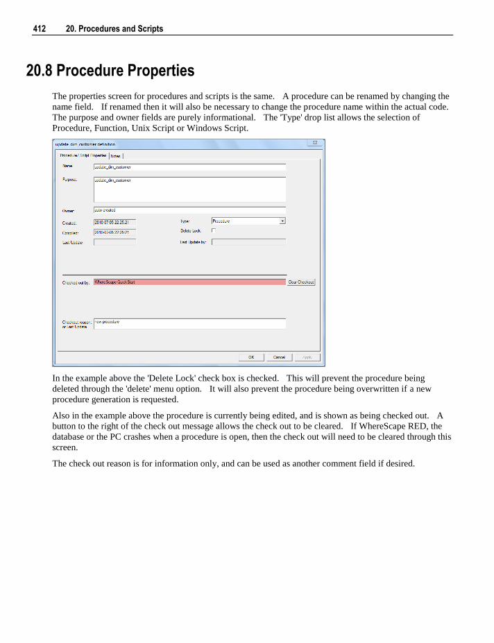
412 20. Procedures and Scripts
20.8 Procedure Properties
The properties screen for procedures and scripts is the same. A procedure can be renamed by changing the
name field. If renamed then it will also be necessary to change the procedure name within the actual code.
The purpose and owner fields are purely informational. The 'Type' drop list allows the selection of
Procedure, Function, Unix Script or Windows Script.
In the example above the 'Delete Lock' check box is checked. This will prevent the procedure being
deleted through the 'delete' menu option. It will also prevent the procedure being overwritten if a new
procedure generation is requested.
Also in the example above the procedure is currently being edited, and is shown as being checked out. A
button to the right of the check out message allows the check out to be cleared. If WhereScape RED, the
database or the PC crashes when a procedure is open, then the check out will need to be cleared through this
screen.
The check out reason is for information only, and can be used as another comment field if desired.
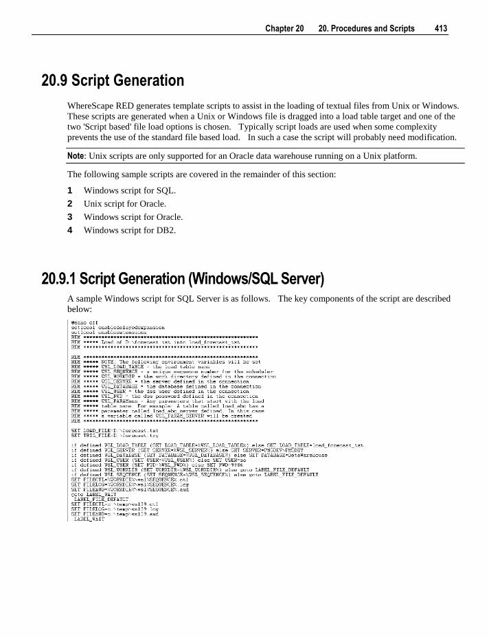
Chapter 20 20. Procedures and Scripts 413
20.9 Script Generation
WhereScape RED generates template scripts to assist in the loading of textual files from Unix or Windows.
These scripts are generated when a Unix or Windows file is dragged into a load table target and one of the
two 'Script based' file load options is chosen. Typically script loads are used when some complexity
prevents the use of the standard file based load. In such a case the script will probably need modification.
Note: Unix scripts are only supported for an Oracle data warehouse running on a Unix platform.
The following sample scripts are covered in the remainder of this section:
1 Windows script for SQL.
2 Unix script for Oracle.
3 Windows script for Oracle.
4 Windows script for DB2.
20.9.1 Script Generation (Windows/SQL Server) A sample Windows script for SQL Server is as follows. The key components of the script are described
below:
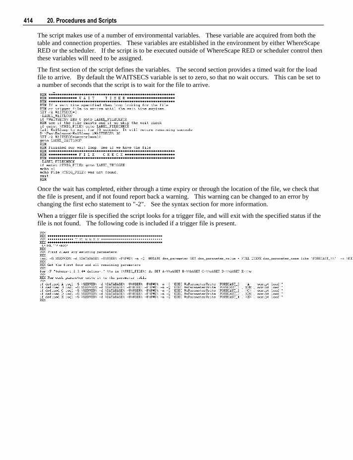
414 20. Procedures and Scripts
The script makes use of a number of environmental variables. These variable are acquired from both the
table and connection properties. These variables are established in the environment by either WhereScape
RED or the scheduler. If the script is to be executed outside of WhereScape RED or scheduler control then
these variables will need to be assigned.
The first section of the script defines the variables. The second section provides a timed wait for the load
file to arrive. By default the WAITSECS variable is set to zero, so that no wait occurs. This can be set to
a number of seconds that the script is to wait for the file to arrive.
Once the wait has completed, either through a time expiry or through the location of the file, we check that
the file is present, and if not found report back a warning. This warning can be changed to an error by
changing the first echo statement to "-2". See the syntax section for more information.
When a trigger file is specified the script looks for a trigger file, and will exit with the specified status if the
file is not found. The following code is included if a trigger file is present.
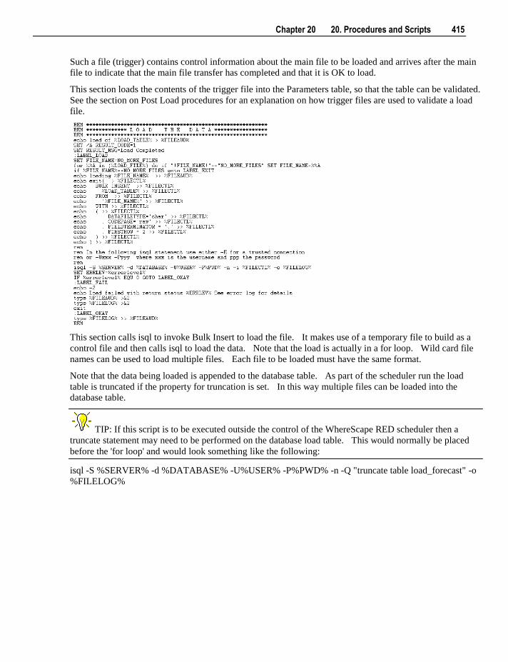
Chapter 20 20. Procedures and Scripts 415
Such a file (trigger) contains control information about the main file to be loaded and arrives after the main
file to indicate that the main file transfer has completed and that it is OK to load.
This section loads the contents of the trigger file into the Parameters table, so that the table can be validated.
See the section on Post Load procedures for an explanation on how trigger files are used to validate a load
file.
This section calls isql to invoke Bulk Insert to load the file. It makes use of a temporary file to build as a
control file and then calls isql to load the data. Note that the load is actually in a for loop. Wild card file
names can be used to load multiple files. Each file to be loaded must have the same format.
Note that the data being loaded is appended to the database table. As part of the scheduler run the load
table is truncated if the property for truncation is set. In this way multiple files can be loaded into the
database table.
TIP: If this script is to be executed outside the control of the WhereScape RED scheduler then a
truncate statement may need to be performed on the database load table. This would normally be placed
before the 'for loop' and would look something like the following:
isql -S %SERVER% -d %DATABASE% -U%USER% -P%PWD% -n -Q "truncate table load_forecast" -o
%FILELOG%
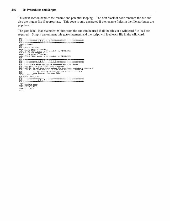
416 20. Procedures and Scripts
This next section handles the rename and potential looping. The first block of code renames the file and
also the trigger file if appropriate. This code is only generated if the rename fields in the file attributes are
populated.
The goto label_load statement 9 lines from the end can be used if all the files in a wild card file load are
required. Simply uncomment this goto statement and the script will load each file in the wild card.

Chapter 20 20. Procedures and Scripts 417
20.9.2 Script Generation (Unix/Oracle) A sample Unix script for Oracle is as follows. The key components of the script are described below:
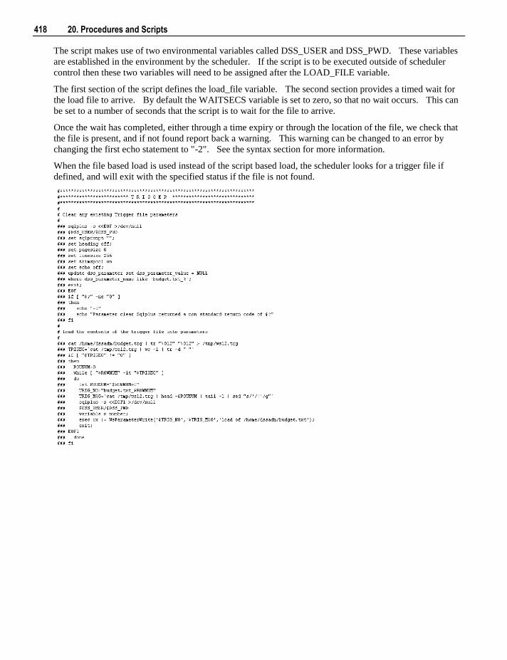
418 20. Procedures and Scripts
The script makes use of two environmental variables called DSS_USER and DSS_PWD. These variables
are established in the environment by the scheduler. If the script is to be executed outside of scheduler
control then these two variables will need to be assigned after the LOAD_FILE variable.
The first section of the script defines the load_file variable. The second section provides a timed wait for
the load file to arrive. By default the WAITSECS variable is set to zero, so that no wait occurs. This can
be set to a number of seconds that the script is to wait for the file to arrive.
Once the wait has completed, either through a time expiry or through the location of the file, we check that
the file is present, and if not found report back a warning. This warning can be changed to an error by
changing the first echo statement to "-2". See the syntax section for more information.
When the file based load is used instead of the script based load, the scheduler looks for a trigger file if
defined, and will exit with the specified status if the file is not found.
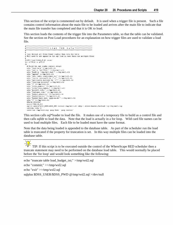
Chapter 20 20. Procedures and Scripts 419
This section of the script is commented out by default. It is used when a trigger file is present. Such a file
contains control information about the main file to be loaded and arrives after the main file to indicate that
the main file transfer has completed and that it is OK to load.
This section loads the contents of the trigger file into the Parameters table, so that the table can be validated.
See the section on Post Load procedures for an explanation on how trigger files are used to validate a load
file.
This section calls sql*loader to load the file. It makes use of a temporary file to build as a control file and
then calls sqlldr to load the data. Note that the load is actually in a for loop. Wild card file names can be
used to load multiple files. Each file to be loaded must have the same format.
Note that the data being loaded is appended to the database table. As part of the scheduler run the load
table is truncated if the property for truncation is set. In this way multiple files can be loaded into the
database table.
TIP: If this script is to be executed outside the control of the WhereScape RED scheduler then a
truncate statement may need to be performed on the database load table. This would normally be placed
before the 'for loop' and would look something like the following:
echo "truncate table load_budget_txt;" >/tmp/wsl2.sql
echo "commit;" >>/tmp/wsl2.sql
echo "exit" >>/tmp/wsl2.sql
sqlplus $DSS_USER/$DSS_PWD @/tmp/wsl2.sql >/dev/null
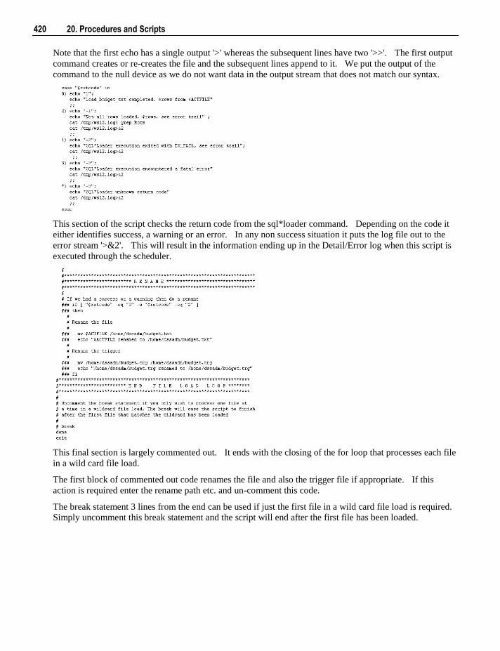
420 20. Procedures and Scripts
Note that the first echo has a single output '>' whereas the subsequent lines have two '>>'. The first output
command creates or re-creates the file and the subsequent lines append to it. We put the output of the
command to the null device as we do not want data in the output stream that does not match our syntax.
This section of the script checks the return code from the sql*loader command. Depending on the code it
either identifies success, a warning or an error. In any non success situation it puts the log file out to the
error stream '>&2'. This will result in the information ending up in the Detail/Error log when this script is
executed through the scheduler.
This final section is largely commented out. It ends with the closing of the for loop that processes each file
in a wild card file load.
The first block of commented out code renames the file and also the trigger file if appropriate. If this
action is required enter the rename path etc. and un-comment this code.
The break statement 3 lines from the end can be used if just the first file in a wild card file load is required.
Simply uncomment this break statement and the script will end after the first file has been loaded.
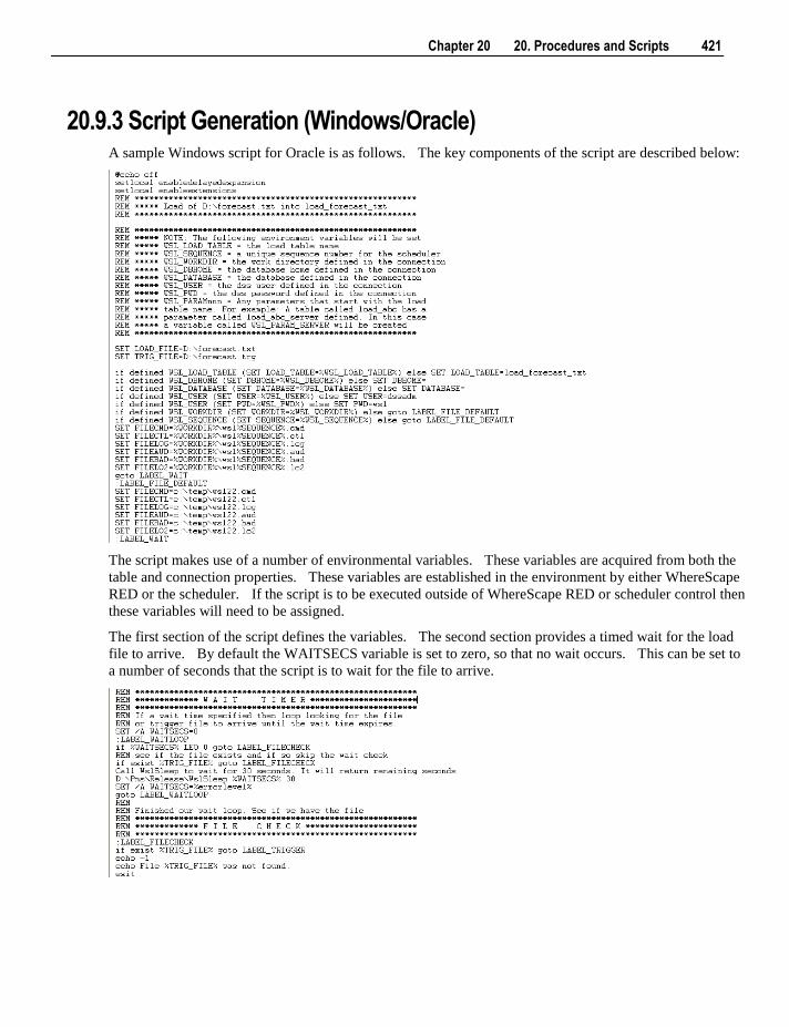
Chapter 20 20. Procedures and Scripts 421
20.9.3 Script Generation (Windows/Oracle) A sample Windows script for Oracle is as follows. The key components of the script are described below:
The script makes use of a number of environmental variables. These variables are acquired from both the
table and connection properties. These variables are established in the environment by either WhereScape
RED or the scheduler. If the script is to be executed outside of WhereScape RED or scheduler control then
these variables will need to be assigned.
The first section of the script defines the variables. The second section provides a timed wait for the load
file to arrive. By default the WAITSECS variable is set to zero, so that no wait occurs. This can be set to
a number of seconds that the script is to wait for the file to arrive.
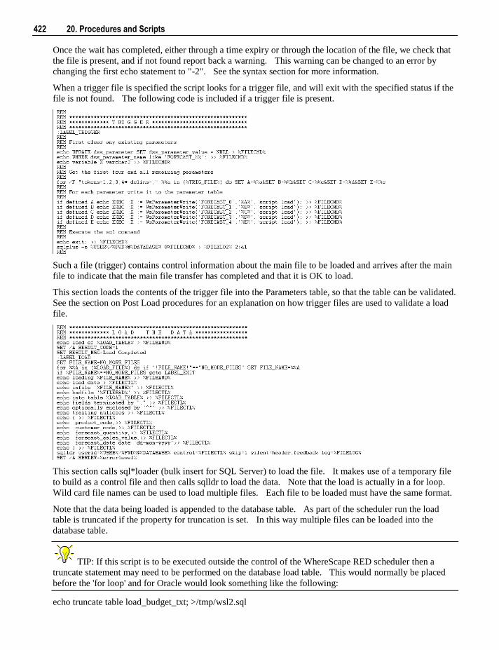
422 20. Procedures and Scripts
Once the wait has completed, either through a time expiry or through the location of the file, we check that
the file is present, and if not found report back a warning. This warning can be changed to an error by
changing the first echo statement to "-2". See the syntax section for more information.
When a trigger file is specified the script looks for a trigger file, and will exit with the specified status if the
file is not found. The following code is included if a trigger file is present.
Such a file (trigger) contains control information about the main file to be loaded and arrives after the main
file to indicate that the main file transfer has completed and that it is OK to load.
This section loads the contents of the trigger file into the Parameters table, so that the table can be validated.
See the section on Post Load procedures for an explanation on how trigger files are used to validate a load
file.
This section calls sql*loader (bulk insert for SQL Server) to load the file. It makes use of a temporary file
to build as a control file and then calls sqlldr to load the data. Note that the load is actually in a for loop.
Wild card file names can be used to load multiple files. Each file to be loaded must have the same format.
Note that the data being loaded is appended to the database table. As part of the scheduler run the load
table is truncated if the property for truncation is set. In this way multiple files can be loaded into the
database table.
TIP: If this script is to be executed outside the control of the WhereScape RED scheduler then a
truncate statement may need to be performed on the database load table. This would normally be placed
before the 'for loop' and for Oracle would look something like the following:
echo truncate table load_budget_txt; >/tmp/wsl2.sql
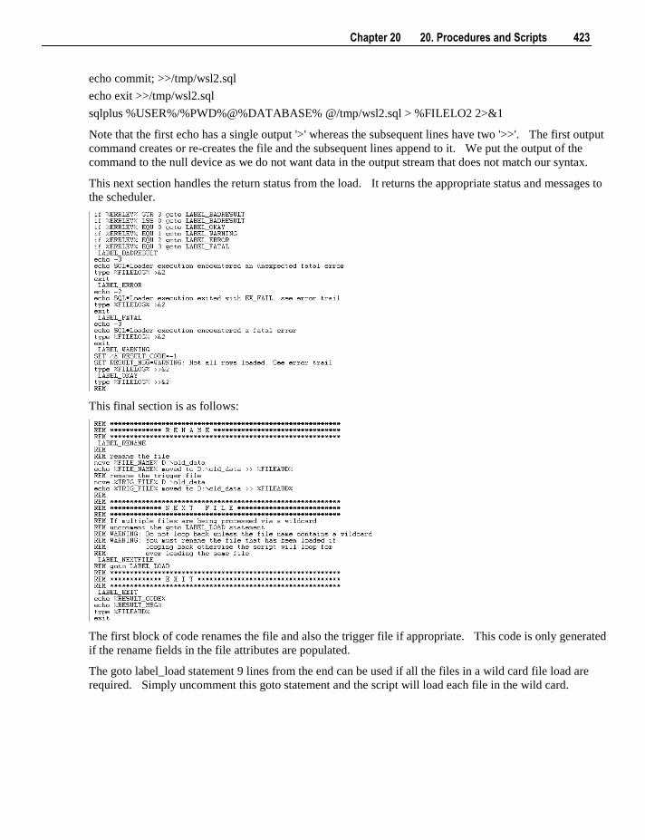
Chapter 20 20. Procedures and Scripts 423
echo commit; >>/tmp/wsl2.sql
echo exit >>/tmp/wsl2.sql
sqlplus %USER%/%PWD%@%DATABASE% @/tmp/wsl2.sql > %FILELO2 2>&1
Note that the first echo has a single output '>' whereas the subsequent lines have two '>>'. The first output
command creates or re-creates the file and the subsequent lines append to it. We put the output of the
command to the null device as we do not want data in the output stream that does not match our syntax.
This next section handles the return status from the load. It returns the appropriate status and messages to
the scheduler.
This final section is as follows:
The first block of code renames the file and also the trigger file if appropriate. This code is only generated
if the rename fields in the file attributes are populated.
The goto label_load statement 9 lines from the end can be used if all the files in a wild card file load are
required. Simply uncomment this goto statement and the script will load each file in the wild card.
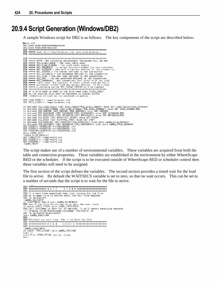
424 20. Procedures and Scripts
20.9.4 Script Generation (Windows/DB2) A sample Windows script for DB2 is as follows. The key components of the script are described below:
The script makes use of a number of environmental variables. These variables are acquired from both the
table and connection properties. These variables are established in the environment by either WhereScape
RED or the scheduler. If the script is to be executed outside of WhereScape RED or scheduler control then
these variables will need to be assigned.
The first section of the script defines the variables. The second section provides a timed wait for the load
file to arrive. By default the WAITSECS variable is set to zero, so that no wait occurs. This can be set to
a number of seconds that the script is to wait for the file to arrive.
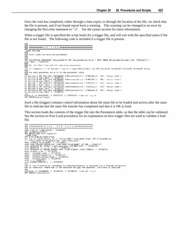
Chapter 20 20. Procedures and Scripts 425
Once the wait has completed, either through a time expiry or through the location of the file, we check that
the file is present, and if not found report back a warning. This warning can be changed to an error by
changing the first echo statement to "-2". See the syntax section for more information.
When a trigger file is specified the script looks for a trigger file, and will exit with the specified status if the
file is not found. The following code is included if a trigger file is present.
Such a file (trigger) contains control information about the main file to be loaded and arrives after the main
file to indicate that the main file transfer has completed and that it is OK to load.
This section loads the contents of the trigger file into the Parameters table, so that the table can be validated.
See the section on Post Load procedures for an explanation on how trigger files are used to validate a load
file.
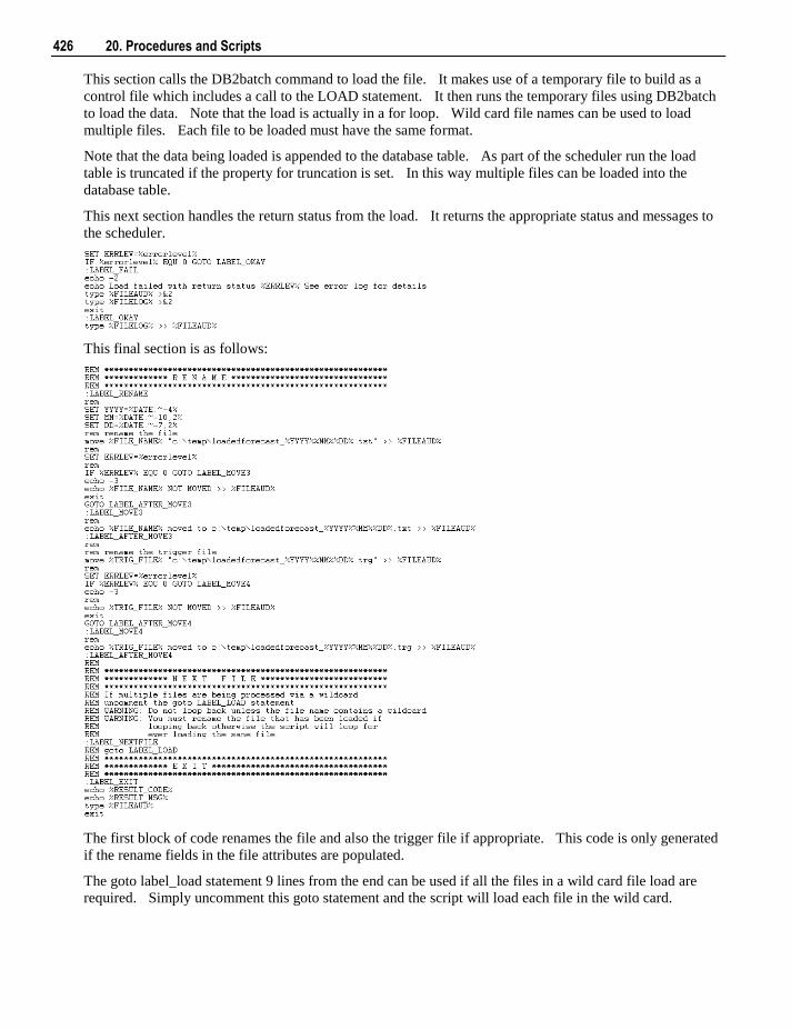
426 20. Procedures and Scripts
This section calls the DB2batch command to load the file. It makes use of a temporary file to build as a
control file which includes a call to the LOAD statement. It then runs the temporary files using DB2batch
to load the data. Note that the load is actually in a for loop. Wild card file names can be used to load
multiple files. Each file to be loaded must have the same format.
Note that the data being loaded is appended to the database table. As part of the scheduler run the load
table is truncated if the property for truncation is set. In this way multiple files can be loaded into the
database table.
This next section handles the return status from the load. It returns the appropriate status and messages to
the scheduler.
This final section is as follows:
The first block of code renames the file and also the trigger file if appropriate. This code is only generated
if the rename fields in the file attributes are populated.
The goto label_load statement 9 lines from the end can be used if all the files in a wild card file load are
required. Simply uncomment this goto statement and the script will load each file in the wild card.
Chapter 20 20. Procedures and Scripts 427
20.10 Script Editing
WhereScape RED includes a script editor which allows the maintenance of any host scripts within the data
warehouse. The editor is invoked by double clicking on a script name in the left hand pane or by selecting
the 'Edit the script' pop-up menu option when a right mouse menu is activated on the script name.
Indenting code
The tab character inserts four spaces into the text. A shift/tab removes four spaces.
Cut, Copy, Paste and Delete
The normal Windows cut, copy, paste and delete functions are available either through the toolbar or via the
right mouse popup menu.
Indenting a block of text
A selected block of text can be indented by four spaces by depressing the tab character. Each tab will
indent by a further four spaces. A shift/tab will remove four spaces from the front of each line in the
selected block.
Viewing other scripts
During the editing process it is possible to pop up a window containing other scripts. This window allows
cut and paste operations. In such a way it can be used as a work area or as a source of code. Select the
Tools/view script or template menu option to bring the viewer window up. A dialog will appear.
A number of drop down list boxes can be chosen from. Once an item is selected the viewer loads the code
and moves to the right hand side of the edit window. The various options are:
Version: A previously saved version of this script. The description and time are shown.
Script: Some other script stored within the WhereScape metadata.
Template: A template script as defined in the WhereScape metadata.
Once an item is chosen the viewer appears on the right hand side of the edit window. The viewer or the
main edit window can receive the focus by clicking the mouse within the appropriate window. Code can
be cut from one window and pasted into the other. Any changes made in the viewer window cannot be
saved.
428 20. Procedures and Scripts
20.11 Script Testing
When a host script is scheduled, it is run in the scheduler environment. Therefore a Unix scheduler must
be available to run a Unix script and only a Windows scheduler can run a Windows script.
It is possible to test a script interactively. For a Windows script this is achieved by running the script on
the current PC. For a Unix script WhereScape RED will attempt to start a telnet window to the Unix host
(as defined in the default connection for the script) and run the script within this telnet window.
A script is invoked via the Execute/Execute the script menu option. The output from the script is shown in
a pop-up dialog box.
Unix Scripts
Unix scripts have the additional execution option being the menu option Execute/ Execute and retain. This
option will create a Telnet window to the Unix host, execute the script, display the results and leave the
Telnet window up. Additional commands or a review of what occurred can then be undertaken directly in
the Telnet window. When completed the Telnet window should be closed to return to the script editor.
Note: A connection must be correctly set-up to support Unix script testing. See the installation manual and
the section on Unix connections.
20.12 Script Syntax
There are a number of conventions that must be followed if a host script is to be used by the WhereScape
scheduler. These conventions are:
1 The first line of data in 'standard out' must contain the resultant status of the script. Valid values are '1'
to indicate success, '-1' to indicate a warning condition occurred but the result is considered a success,
'-2' to indicate a handled error occurred and subsequent dependent tasks should be held, -3 to indicate
an unhandled Failure and that subsequent dependent tasks should be held.
2 The second line of data in 'standard out' must contain a resultant message of no more than 256
characters.
3 Any subsequent lines in 'standard out' are considered informational and are recorded in the audit trail.
The normal practice is to place a minimum of information in the audit trail. All bulk information
should be output to 'standard error'.
4 Any data output to 'standard error' will be written to the error/detail log. Both the audit log and detail
log can be viewed from the WhereScape RED tool under the scheduler window.
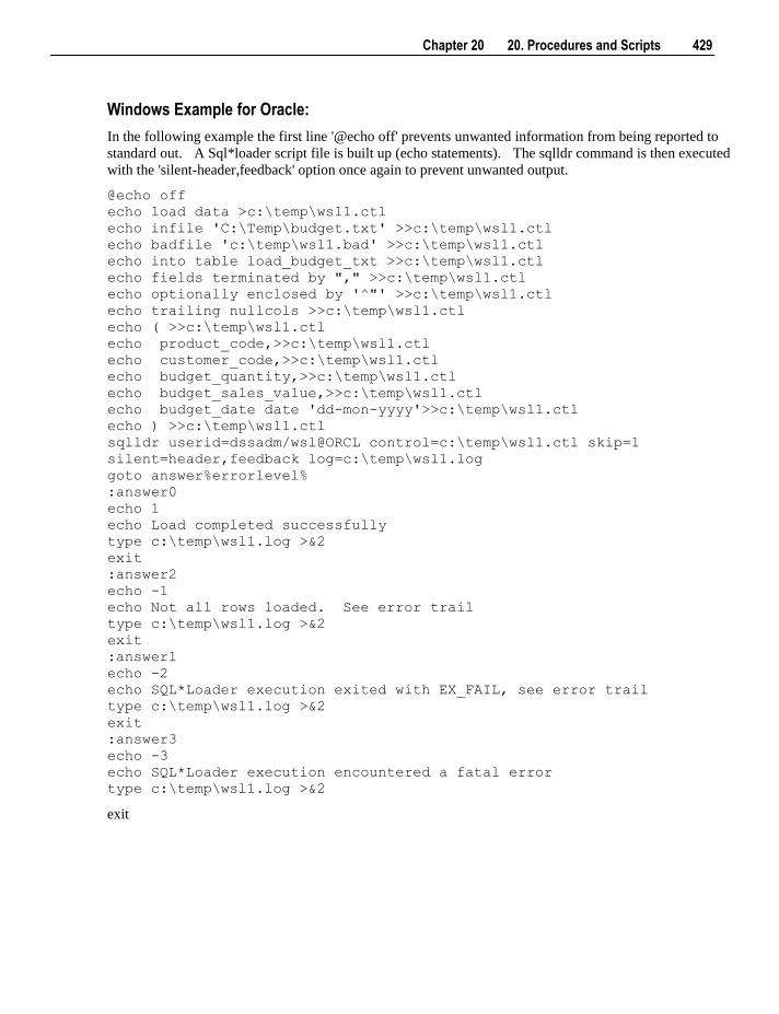
Chapter 20 20. Procedures and Scripts 429
Windows Example for Oracle:
In the following example the first line '@echo off' prevents unwanted information from being reported to
standard out. A Sql*loader script file is built up (echo statements). The sqlldr command is then executed
with the 'silent-header,feedback' option once again to prevent unwanted output.
@echo off
echo load data >c:\temp\wsl1.ctl
echo infile 'C:\Temp\budget.txt' >>c:\temp\wsl1.ctl
echo badfile 'c:\temp\wsl1.bad' >>c:\temp\wsl1.ctl
echo into table load_budget_txt >>c:\temp\wsl1.ctl
echo fields terminated by "," >>c:\temp\wsl1.ctl
echo optionally enclosed by '^"' >>c:\temp\wsl1.ctl
echo trailing nullcols >>c:\temp\wsl1.ctl
echo ( >>c:\temp\wsl1.ctl
echo product_code,>>c:\temp\wsl1.ctl
echo customer_code,>>c:\temp\wsl1.ctl
echo budget_quantity,>>c:\temp\wsl1.ctl
echo budget_sales_value,>>c:\temp\wsl1.ctl
echo budget_date date 'dd-mon-yyyy'>>c:\temp\wsl1.ctl
echo ) >>c:\temp\wsl1.ctl
sqlldr userid=dssadm/wsl@ORCL control=c:\temp\wsl1.ctl skip=1
silent=header,feedback log=c:\temp\wsl1.log
goto answer%errorlevel%
:answer0
echo 1
echo Load completed successfully
type c:\temp\wsl1.log >&2
exit
:answer2
echo -1
echo Not all rows loaded. See error trail
type c:\temp\wsl1.log >&2
exit
:answer1
echo -2
echo SQL*Loader execution exited with EX_FAIL, see error trail
type c:\temp\wsl1.log >&2
exit
:answer3
echo -3
echo SQL*Loader execution encountered a fatal error
type c:\temp\wsl1.log >&2
exit
430 20. Procedures and Scripts
20.13 Templates
Templates serve two main purposes. Firstly they provide a structure for the building of procedures and
scripts. Secondly they provide example code to illustrate how to handle a specific application problem.
A simple template editor is provided to allow the maintenance of templates. Templates are normally either
procedure or host script examples. The normal practice is to develop the template within either the
procedure or script editor and then paste it into the template for storage.
Procedure Structure Templates
These templates are normally only defined at initial setup, and are in fact not visible or accessible in this
version of WhereScape RED.
Example Templates
WhereScape RED ships with a number of example templates to illustrate such situations as set based
updates, pseudo dimension key generation, and job dependencies. A special template called ToDo is also
shipped. This ToDo template provides a To Do list that can be accessed directly from the main browser
window via the appropriate icon. Example templates are also available at the WhereScape web site
http://www.wherescape.com
Submitting Example Templates
WhereScape welcomes the supply of new templates. If you develop custom code that you believe may be
of value to other WhereScape RED users, please feel free to email a copy to [email protected]
Author identities will be acknowledged.
Chapter 21 21. Scheduler 431
The scheduler is accessible by clicking the scheduler button on the toolbar. It is also
available as a stand alone utility. In this way operators can be given access to the scheduler without
gaining full access to the data warehouse.
The scheduler runs on either a Unix host or under Windows ( as a system service ). It processes
pre-defined jobs, recording the success, failure or otherwise of the job.
Audit trail
Specific information relating to the tasks in the job are recorded to the audit trail. Generally only summary
information is written to this audit trail. The contents of the audit trail are maintained even after a job is
deleted.
Error trail
Detail or error information is written to the error trail. The contents of the error trail are deleted when the
job is deleted.
Administration Views
It is possible to view the status of a job without using the WhereScape RED product. Three views are
provided to assist in this undertaking. They are ws_admin_v_audit, ws_admin_v_error and
ws_admin_v_sched. Queries can be issued using these views to see the results or status of a job.
In This Chapter
21.1 Scheduler Options ............................................................... 432
21.2 Scheduler States .................................................................. 435
21.3 Scheduling a Job ................................................................. 437
21.4 Editing Jobs ......................................................................... 445
21.5 Deleting Job Logs ............................................................... 446
21.6 Monitoring the Database and Jobs ...................................... 447
21.7 Stand Alone Scheduler Maintenance .................................. 454
C H A P T E R 2 1
21. Scheduler
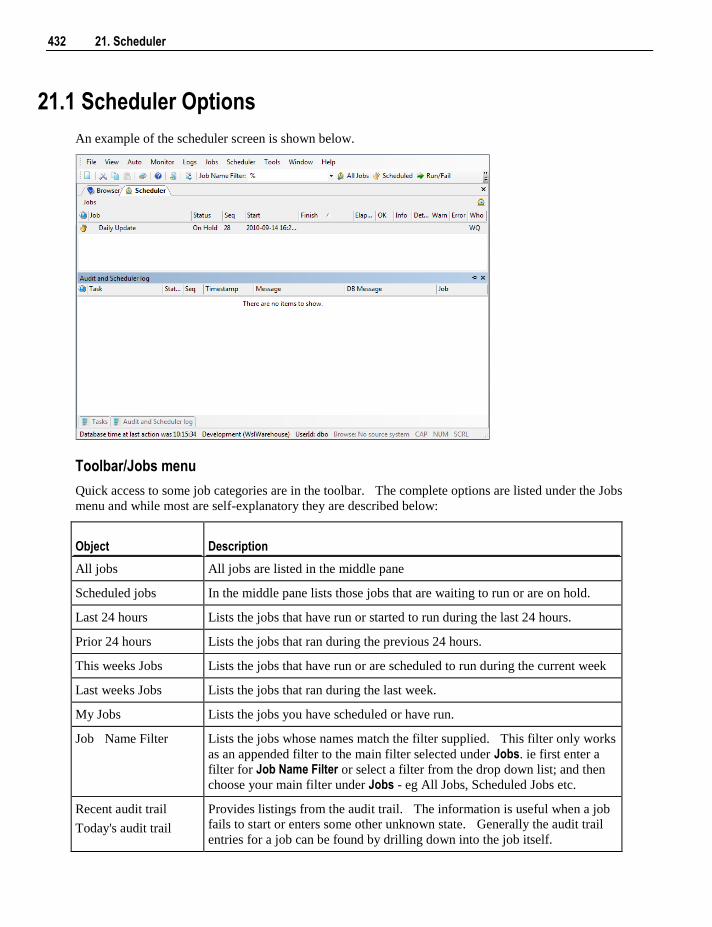
432 21. Scheduler
21.1 Scheduler Options
An example of the scheduler screen is shown below.
Toolbar/Jobs menu
Quick access to some job categories are in the toolbar. The complete options are listed under the Jobs
menu and while most are self-explanatory they are described below:
Object Description
All jobs All jobs are listed in the middle pane
Scheduled jobs In the middle pane lists those jobs that are waiting to run or are on hold.
Last 24 hours Lists the jobs that have run or started to run during the last 24 hours.
Prior 24 hours Lists the jobs that ran during the previous 24 hours.
This weeks Jobs Lists the jobs that have run or are scheduled to run during the current week
Last weeks Jobs Lists the jobs that ran during the last week.
My Jobs Lists the jobs you have scheduled or have run.
Job Name Filter Lists the jobs whose names match the filter supplied. This filter only works
as an appended filter to the main filter selected under Jobs. ie first enter a
filter for Job Name Filter or select a filter from the drop down list; and then
choose your main filter under Jobs - eg All Jobs, Scheduled Jobs etc.
Recent audit trail
Today's audit trail
Provides listings from the audit trail. The information is useful when a job
fails to start or enters some other unknown state. Generally the audit trail
entries for a job can be found by drilling down into the job itself.
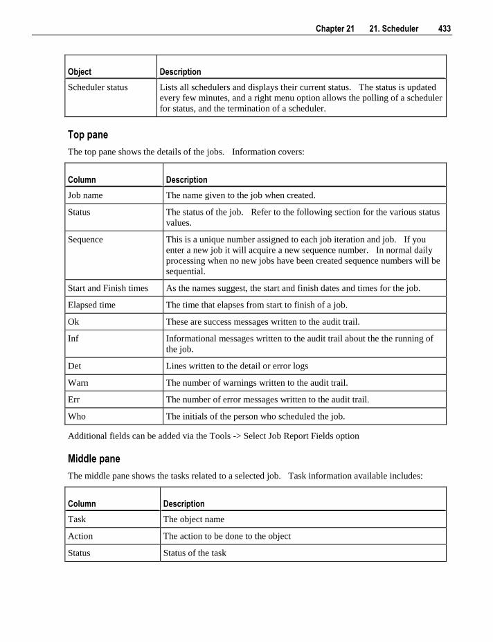
Chapter 21 21. Scheduler 433
Object Description
Scheduler status Lists all schedulers and displays their current status. The status is updated
every few minutes, and a right menu option allows the polling of a scheduler
for status, and the termination of a scheduler.
Top pane
The top pane shows the details of the jobs. Information covers:
Column Description
Job name The name given to the job when created.
Status The status of the job. Refer to the following section for the various status
values.
Sequence This is a unique number assigned to each job iteration and job. If you
enter a new job it will acquire a new sequence number. In normal daily
processing when no new jobs have been created sequence numbers will be
sequential.
Start and Finish times As the names suggest, the start and finish dates and times for the job.
Elapsed time The time that elapses from start to finish of a job.
Ok These are success messages written to the audit trail.
Inf Informational messages written to the audit trail about the the running of
the job.
Det Lines written to the detail or error logs
Warn The number of warnings written to the audit trail.
Err The number of error messages written to the audit trail.
Who The initials of the person who scheduled the job.
Additional fields can be added via the Tools -> Select Job Report Fields option
Middle pane
The middle pane shows the tasks related to a selected job. Task information available includes:
Column Description
Task The object name
Action The action to be done to the object
Status Status of the task
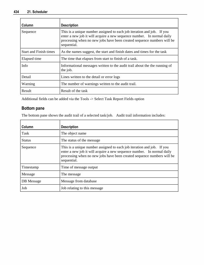
434 21. Scheduler
Column Description
Sequence This is a unique number assigned to each job iteration and job. If you
enter a new job it will acquire a new sequence number. In normal daily
processing when no new jobs have been created sequence numbers will be
sequential.
Start and Finish times As the names suggest, the start and finish dates and times for the task
Elapsed time The time that elapses from start to finish of a task.
Info Informational messages written to the audit trail about the the running of
the job.
Detail Lines written to the detail or error logs
Warning The number of warnings written to the audit trail.
Result Result of the task
Additional fields can be added via the Tools -> Select Task Report Fields option
Bottom pane
The bottom pane shows the audit trail of a selected task/job. Audit trail information includes:
Column Description
Task The object name
Status The status of the message
Sequence This is a unique number assigned to each job iteration and job. If you
enter a new job it will acquire a new sequence number. In normal daily
processing when no new jobs have been created sequence numbers will be
sequential.
Timestamp Time of message output
Message The message
DB Message Message from database
Job Job relating to this message
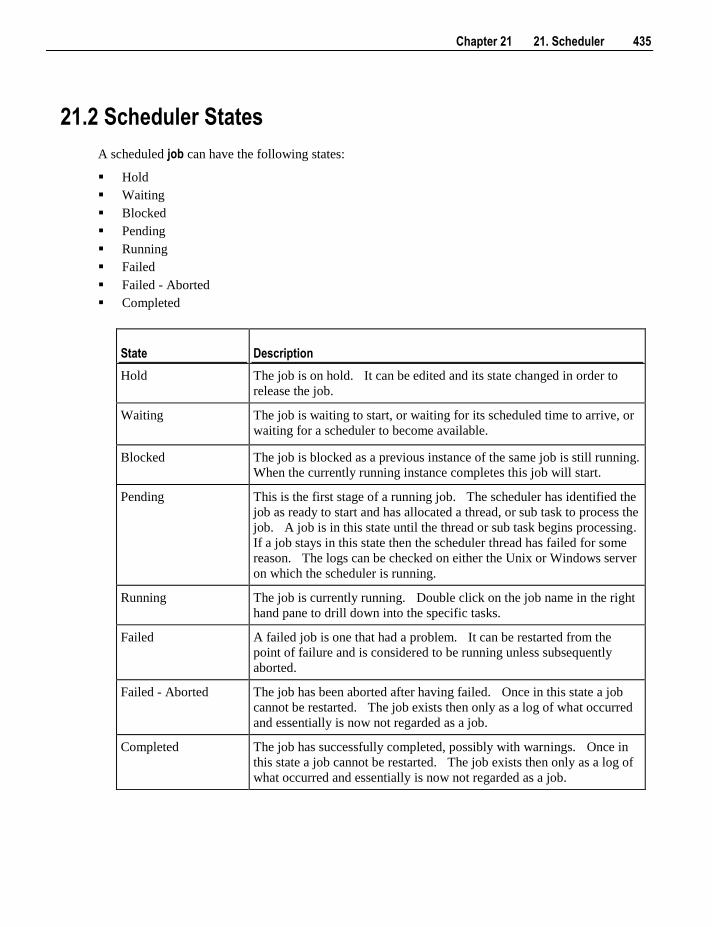
Chapter 21 21. Scheduler 435
21.2 Scheduler States
A scheduled job can have the following states:
Hold
Waiting
Blocked
Pending
Running
Failed
Failed - Aborted
Completed
State Description
Hold The job is on hold. It can be edited and its state changed in order to
release the job.
Waiting
The job is waiting to start, or waiting for its scheduled time to arrive, or
waiting for a scheduler to become available.
Blocked The job is blocked as a previous instance of the same job is still running.
When the currently running instance completes this job will start.
Pending This is the first stage of a running job. The scheduler has identified the
job as ready to start and has allocated a thread, or sub task to process the
job. A job is in this state until the thread or sub task begins processing.
If a job stays in this state then the scheduler thread has failed for some
reason. The logs can be checked on either the Unix or Windows server
on which the scheduler is running.
Running The job is currently running. Double click on the job name in the right
hand pane to drill down into the specific tasks.
Failed A failed job is one that had a problem. It can be restarted from the
point of failure and is considered to be running unless subsequently
aborted.
Failed - Aborted The job has been aborted after having failed. Once in this state a job
cannot be restarted. The job exists then only as a log of what occurred
and essentially is now not regarded as a job.
Completed The job has successfully completed, possibly with warnings. Once in
this state a job cannot be restarted. The job exists then only as a log of
what occurred and essentially is now not regarded as a job.
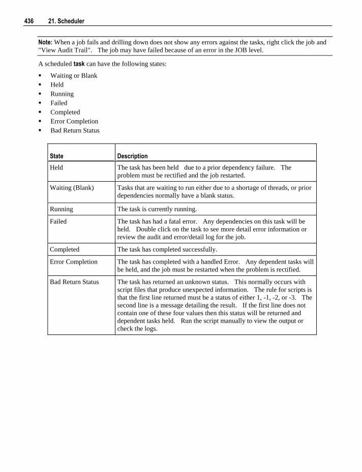
436 21. Scheduler
Note: When a job fails and drilling down does not show any errors against the tasks, right click the job and
"View Audit Trail". The job may have failed because of an error in the JOB level.
A scheduled task can have the following states:
Waiting or Blank
Held
Running
Failed
Completed
Error Completion
Bad Return Status
State Description
Held The task has been held due to a prior dependency failure. The
problem must be rectified and the job restarted.
Waiting (Blank)
Tasks that are waiting to run either due to a shortage of threads, or prior
dependencies normally have a blank status.
Running The task is currently running.
Failed The task has had a fatal error. Any dependencies on this task will be
held. Double click on the task to see more detail error information or
review the audit and error/detail log for the job.
Completed The task has completed successfully.
Error Completion The task has completed with a handled Error. Any dependent tasks will
be held, and the job must be restarted when the problem is rectified.
Bad Return Status The task has returned an unknown status. This normally occurs with
script files that produce unexpected information. The rule for scripts is
that the first line returned must be a status of either 1, -1, -2, or -3. The
second line is a message detailing the result. If the first line does not
contain one of these four values then this status will be returned and
dependent tasks held. Run the script manually to view the output or
check the logs.
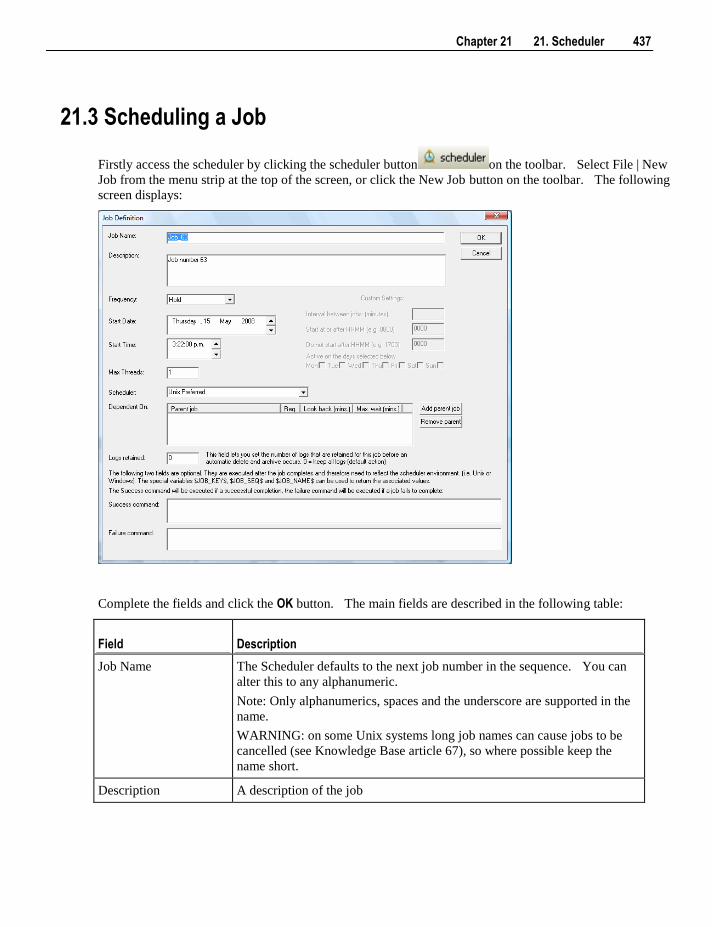
Chapter 21 21. Scheduler 437
21.3 Scheduling a Job
Firstly access the scheduler by clicking the scheduler button on the toolbar. Select File | New
Job from the menu strip at the top of the screen, or click the New Job button on the toolbar. The following
screen displays:
Complete the fields and click the OK button. The main fields are described in the following table:
Field Description
Job Name The Scheduler defaults to the next job number in the sequence. You can
alter this to any alphanumeric.
Note: Only alphanumerics, spaces and the underscore are supported in the
name.
WARNING: on some Unix systems long job names can cause jobs to be
cancelled (see Knowledge Base article 67), so where possible keep the
name short.
Description A description of the job
438 21. Scheduler
Field Description
Frequency When the job runs. The options available in the drop down list box are:
Once Only - job is deleted on completion
Once and Hold - runs and puts another copy of the job on hold
Hold - puts the job on hold for manual release
Daily - runs the job daily
Custom - enables custom definition
Weekly - runs the job weekly
Monthly - runs the job monthly
Annually - runs the job annually
Start Date and Start
Time
The date and time for the job to start.
Max Threads The maximum number of threads allocated to run the job, e.g, if some tasks
can run in parallel then if more than one thread is allocated then they will
run in parallel.
Scheduler Certain types of job will only run in a specific environment. For example
ODBC based loads can only be handled by the Windows' scheduler. It is
possible to have multiple schedulers running. Select the desired scheduler
from this drop down. The valid options are:
Unix Preferred, Unix Only, Windows Preferred, Windows Only, or the
name of a specific scheduler can be entered (e.g. WIN0002)
Dependent On A job can be dependent on the successful completion of one or more other
jobs. Click the 'Add Parent Job' button to select a job that this job will be
dependent on. The maximum time to look back for parent job completion
field prevents older iterations of the parent job as being identified as a
completion. The maximum time to wait specifies how long to await a
successful completion of the parent job. The action if that wait expires can
also be set.
Logs Retained Specify the number of logs to retain for the job. By default all logs are
retained. This field can be used to reduce the build up of scheduler logs by
specifying a number of logs to retain.
OK command and
Failure command
These are either Unix or Windows shell commands depending on which
scheduler is used. They are executed if the condition is met. Typically,
these commands would mail or page on success or failure.
The following fields are available if a frequency of Custom is chosen:
Field Description
Interval between jobs
(Minutes)
Specify the number of minutes between iterations of the job. For example
to run a job every 30 minutes set this value to 30. If a job is to run only
once but on selected days set this value to 1440 (daily)
Start at or after HHMM The time that the job may run from. To run anytime set to 0000.
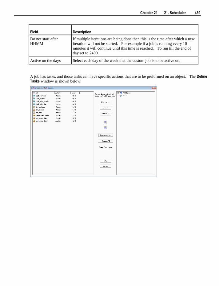
Chapter 21 21. Scheduler 439
Field Description
Do not start after
HHMM
If multiple iterations are being done then this is the time after which a new
iteration will not be started. For example if a job is running every 10
minutes it will continue until this time is reached. To run till the end of
day set to 2400.
Active on the days Select each day of the week that the custom job is to be active on.
A job has tasks, and those tasks can have specific actions that are to be performed on an object. The Define Tasks window is shown below:
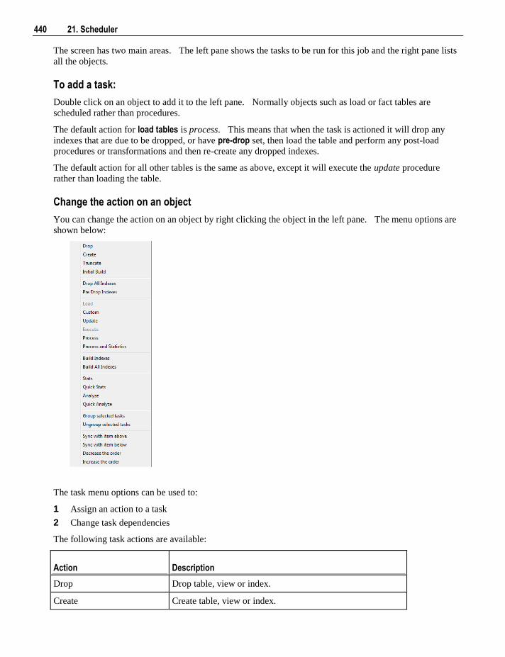
440 21. Scheduler
The screen has two main areas. The left pane shows the tasks to be run for this job and the right pane lists
all the objects.
To add a task:
Double click on an object to add it to the left pane. Normally objects such as load or fact tables are
scheduled rather than procedures.
The default action for load tables is process. This means that when the task is actioned it will drop any
indexes that are due to be dropped, or have pre-drop set, then load the table and perform any post-load
procedures or transformations and then re-create any dropped indexes.
The default action for all other tables is the same as above, except it will execute the update procedure
rather than loading the table.
Change the action on an object
You can change the action on an object by right clicking the object in the left pane. The menu options are
shown below:
The task menu options can be used to:
1 Assign an action to a task
2 Change task dependencies
The following task actions are available:
Action Description
Drop Drop table, view or index.
Create Create table, view or index.
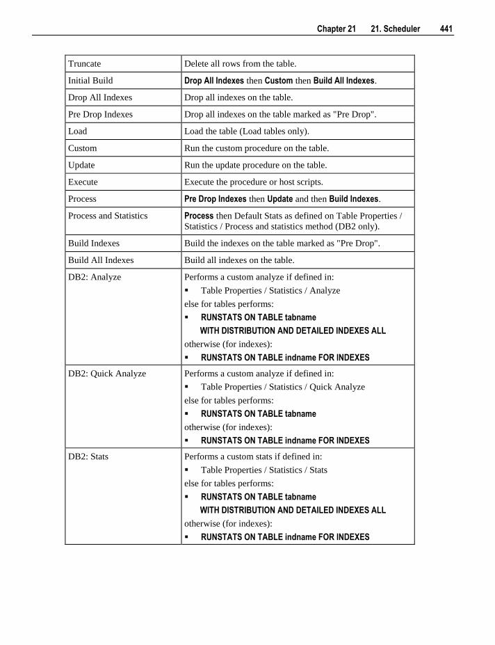
Chapter 21 21. Scheduler 441
Truncate Delete all rows from the table.
Initial Build Drop All Indexes then Custom then Build All Indexes.
Drop All Indexes Drop all indexes on the table.
Pre Drop Indexes Drop all indexes on the table marked as "Pre Drop".
Load Load the table (Load tables only).
Custom Run the custom procedure on the table.
Update Run the update procedure on the table.
Execute Execute the procedure or host scripts.
Process Pre Drop Indexes then Update and then Build Indexes.
Process and Statistics Process then Default Stats as defined on Table Properties /
Statistics / Process and statistics method (DB2 only).
Build Indexes Build the indexes on the table marked as "Pre Drop".
Build All Indexes Build all indexes on the table.
DB2: Analyze Performs a custom analyze if defined in:
Table Properties / Statistics / Analyze
else for tables performs:
RUNSTATS ON TABLE tabname
WITH DISTRIBUTION AND DETAILED INDEXES ALL
otherwise (for indexes):
RUNSTATS ON TABLE indname FOR INDEXES
DB2: Quick Analyze Performs a custom analyze if defined in:
Table Properties / Statistics / Quick Analyze
else for tables performs:
RUNSTATS ON TABLE tabname
otherwise (for indexes):
RUNSTATS ON TABLE indname FOR INDEXES
DB2: Stats Performs a custom stats if defined in:
Table Properties / Statistics / Stats
else for tables performs:
RUNSTATS ON TABLE tabname
WITH DISTRIBUTION AND DETAILED INDEXES ALL
otherwise (for indexes):
RUNSTATS ON TABLE indname FOR INDEXES
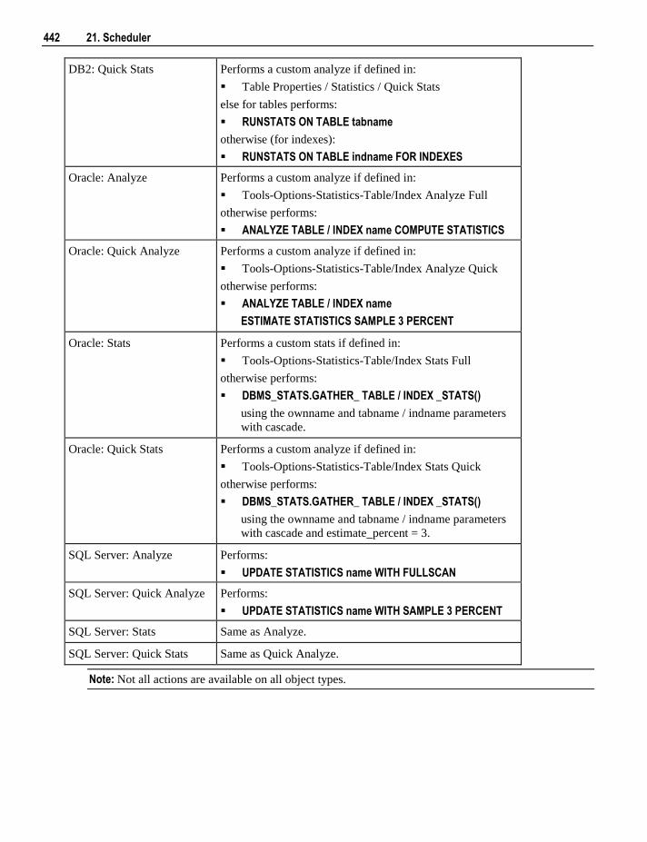
442 21. Scheduler
DB2: Quick Stats Performs a custom analyze if defined in:
Table Properties / Statistics / Quick Stats
else for tables performs:
RUNSTATS ON TABLE tabname
otherwise (for indexes):
RUNSTATS ON TABLE indname FOR INDEXES
Oracle: Analyze Performs a custom analyze if defined in:
Tools-Options-Statistics-Table/Index Analyze Full
otherwise performs:
ANALYZE TABLE / INDEX name COMPUTE STATISTICS
Oracle: Quick Analyze Performs a custom analyze if defined in:
Tools-Options-Statistics-Table/Index Analyze Quick
otherwise performs:
ANALYZE TABLE / INDEX name
ESTIMATE STATISTICS SAMPLE 3 PERCENT
Oracle: Stats Performs a custom stats if defined in:
Tools-Options-Statistics-Table/Index Stats Full
otherwise performs:
DBMS_STATS.GATHER_ TABLE / INDEX _STATS()
using the ownname and tabname / indname parameters
with cascade.
Oracle: Quick Stats Performs a custom analyze if defined in:
Tools-Options-Statistics-Table/Index Stats Quick
otherwise performs:
DBMS_STATS.GATHER_ TABLE / INDEX _STATS()
using the ownname and tabname / indname parameters
with cascade and estimate_percent = 3.
SQL Server: Analyze Performs:
UPDATE STATISTICS name WITH FULLSCAN
SQL Server: Quick Analyze Performs:
UPDATE STATISTICS name WITH SAMPLE 3 PERCENT
SQL Server: Stats Same as Analyze.
SQL Server: Quick Stats Same as Quick Analyze.
Note: Not all actions are available on all object types.
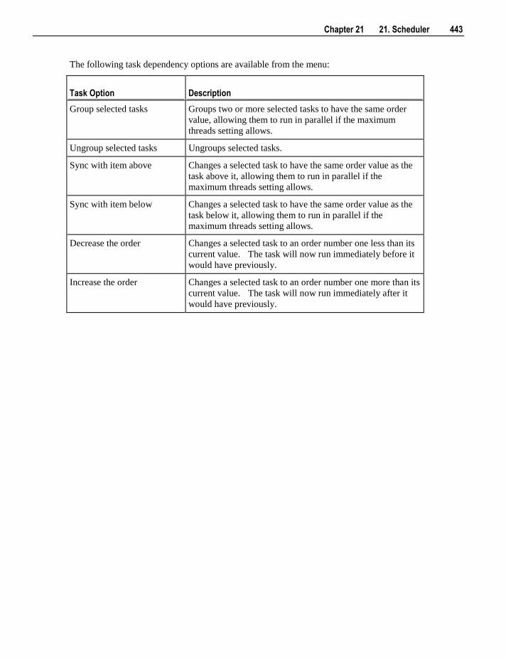
Chapter 21 21. Scheduler 443
The following task dependency options are available from the menu:
Task Option Description
Group selected tasks Groups two or more selected tasks to have the same order
value, allowing them to run in parallel if the maximum
threads setting allows.
Ungroup selected tasks Ungroups selected tasks.
Sync with item above Changes a selected task to have the same order value as the
task above it, allowing them to run in parallel if the
maximum threads setting allows.
Sync with item below Changes a selected task to have the same order value as the
task below it, allowing them to run in parallel if the
maximum threads setting allows.
Decrease the order Changes a selected task to an order number one less than its
current value. The task will now run immediately before it
would have previously.
Increase the order Changes a selected task to an order number one more than its
current value. The task will now run immediately after it
would have previously.
444 21. Scheduler
Order
The order column shows the order in which the tasks are to be run, e.g, 20.20 If the two numbers are the
same as another task then those tasks can run in parallel. If the two numbers are different then those tasks
run sequentially. This is an initial definition of dependencies. These dependencies can be altered
specifically once the job has been created. (An example of dependency editing is provided in Tutorial 3).
Tasks can be moved up or down by selecting the task and clicking the Move Up or Move Down
buttons.
Respace Order
This button will respace the order numbers. The existing dependency structure and groupings are retained.
The purpose of this button is simply to allow room between tasks to fit new tasks. So for example if we
have two tasks that have an order of 20.19.5 and 20.20.6 and we want to add a task between these two tasks
we can click the 'Respace Order' button to open up a gap between the two tasks.
Ungroup All
This button will remove all groupings and make all tasks sequential. New groupings can be made by
selecting a range of sequentially listed tasks in the left hand pane and using the right mouse menu option
'Group selected tasks'. Tasks that are grouped have the same first two numbers in the order and can
execute at the same time if the job has multiple threads.
Group Object Types
This option will put all objects of the same type into groups. For example all load tables will be able to run
in parallel, all dimensions etc.
Jobs within Jobs
It is possible to schedule one job from another job. There are however some limitations and rules that must
be understood when doing this.
1 A job that is called from another job is only ever allocated one thread. All tasks within the called job
will therefore run sequentially.
2 A job can only have one running iteration. Therefore a called job will be blocked if that job is already
running independently or as part of another job.
3 Any job dependencies for the called job are ignored. The parent's job dependencies are the only ones
that are used.
4 A called job essentially runs as a separate job, so that if it fails both it and the parent job will show in a
failed state. Once the problem is fixed the parent job should be restarted which will restart the called
job.
Upon completion of adding tasks click the OK button.
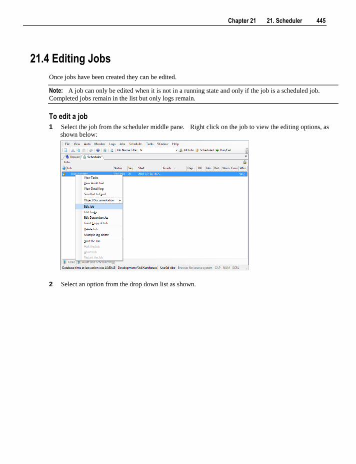
Chapter 21 21. Scheduler 445
21.4 Editing Jobs
Once jobs have been created they can be edited.
Note: A job can only be edited when it is not in a running state and only if the job is a scheduled job.
Completed jobs remain in the list but only logs remain.
To edit a job
1 Select the job from the scheduler middle pane. Right click on the job to view the editing options, as
shown below:
2 Select an option from the drop down list as shown.
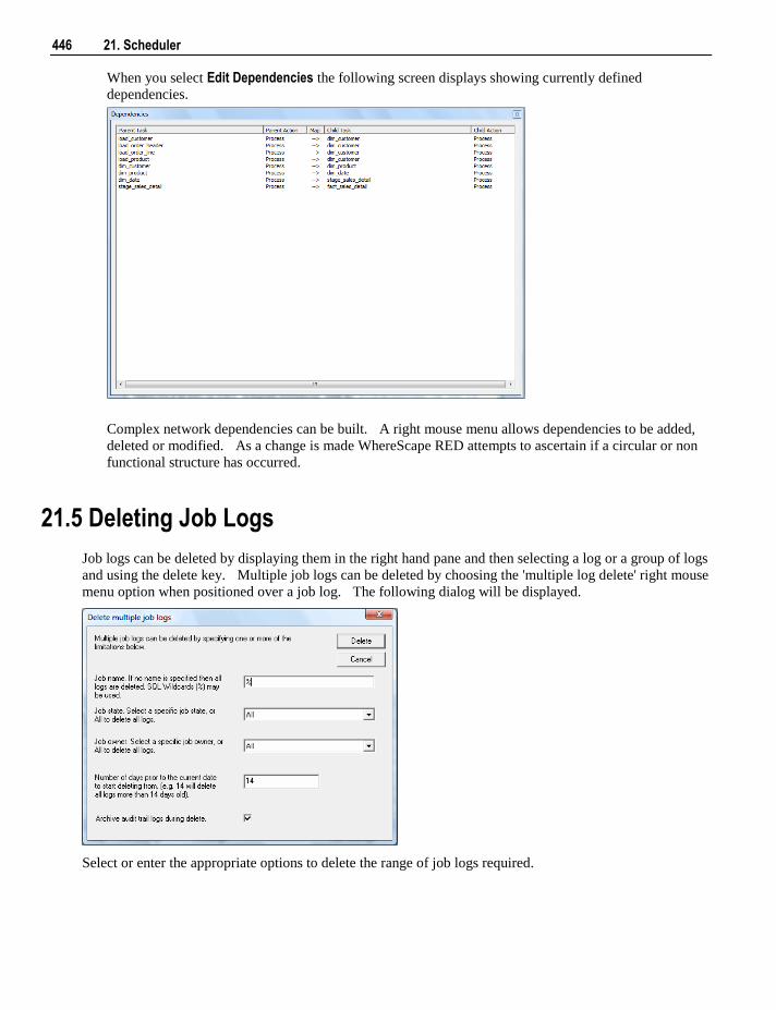
446 21. Scheduler
When you select Edit Dependencies the following screen displays showing currently defined
dependencies.
Complex network dependencies can be built. A right mouse menu allows dependencies to be added,
deleted or modified. As a change is made WhereScape RED attempts to ascertain if a circular or non
functional structure has occurred.
21.5 Deleting Job Logs
Job logs can be deleted by displaying them in the right hand pane and then selecting a log or a group of logs
and using the delete key. Multiple job logs can be deleted by choosing the 'multiple log delete' right mouse
menu option when positioned over a job log. The following dialog will be displayed.
Select or enter the appropriate options to delete the range of job logs required.
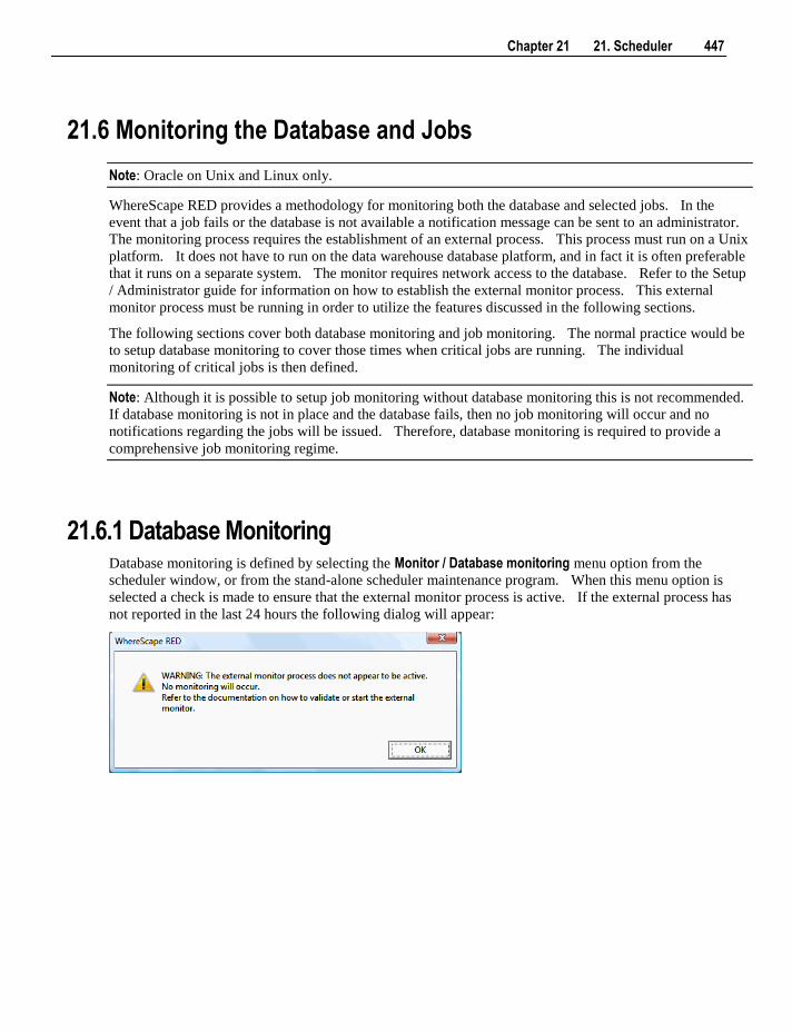
Chapter 21 21. Scheduler 447
21.6 Monitoring the Database and Jobs
Note: Oracle on Unix and Linux only.
WhereScape RED provides a methodology for monitoring both the database and selected jobs. In the
event that a job fails or the database is not available a notification message can be sent to an administrator.
The monitoring process requires the establishment of an external process. This process must run on a Unix
platform. It does not have to run on the data warehouse database platform, and in fact it is often preferable
that it runs on a separate system. The monitor requires network access to the database. Refer to the Setup
/ Administrator guide for information on how to establish the external monitor process. This external
monitor process must be running in order to utilize the features discussed in the following sections.
The following sections cover both database monitoring and job monitoring. The normal practice would be
to setup database monitoring to cover those times when critical jobs are running. The individual
monitoring of critical jobs is then defined.
Note: Although it is possible to setup job monitoring without database monitoring this is not recommended.
If database monitoring is not in place and the database fails, then no job monitoring will occur and no
notifications regarding the jobs will be issued. Therefore, database monitoring is required to provide a
comprehensive job monitoring regime.
21.6.1 Database Monitoring Database monitoring is defined by selecting the Monitor / Database monitoring menu option from the
scheduler window, or from the stand-alone scheduler maintenance program. When this menu option is
selected a check is made to ensure that the external monitor process is active. If the external process has
not reported in the last 24 hours the following dialog will appear:
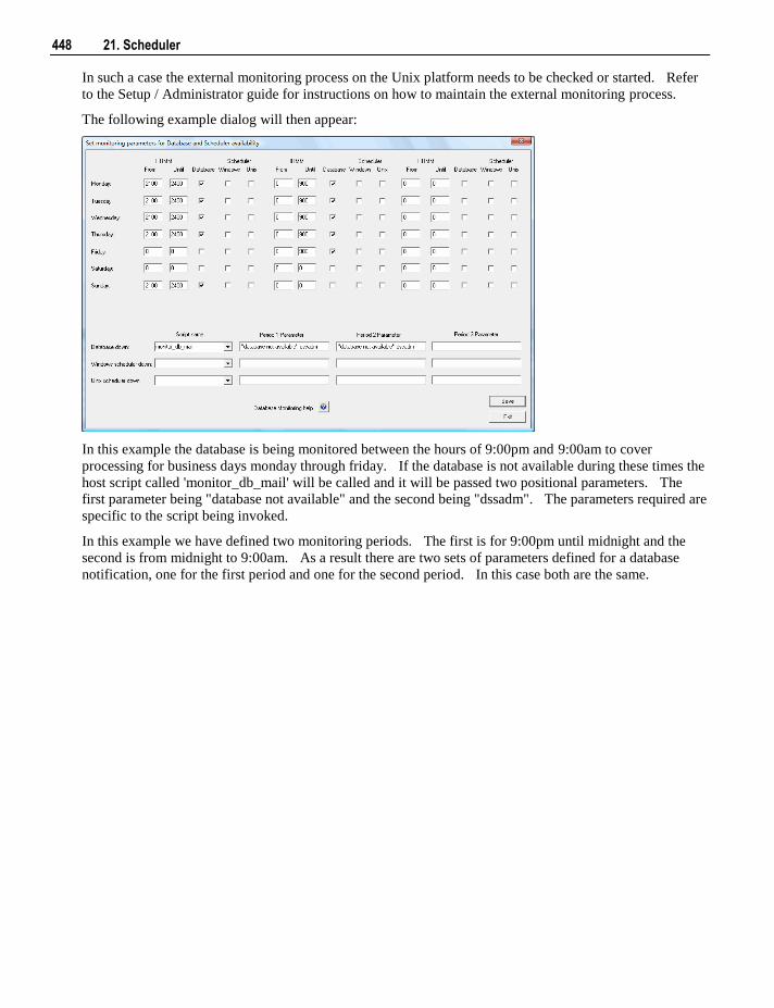
448 21. Scheduler
In such a case the external monitoring process on the Unix platform needs to be checked or started. Refer
to the Setup / Administrator guide for instructions on how to maintain the external monitoring process.
The following example dialog will then appear:
In this example the database is being monitored between the hours of 9:00pm and 9:00am to cover
processing for business days monday through friday. If the database is not available during these times the
host script called 'monitor_db_mail' will be called and it will be passed two positional parameters. The
first parameter being "database not available" and the second being "dssadm". The parameters required are
specific to the script being invoked.
In this example we have defined two monitoring periods. The first is for 9:00pm until midnight and the
second is from midnight to 9:00am. As a result there are two sets of parameters defined for a database
notification, one for the first period and one for the second period. In this case both are the same.
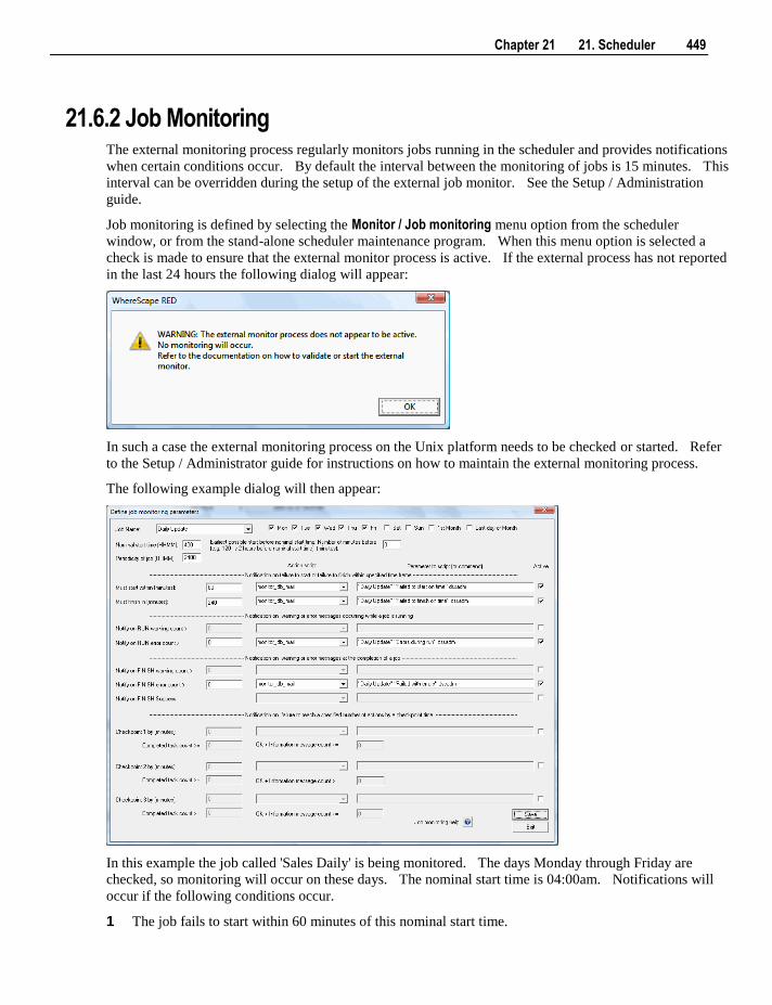
Chapter 21 21. Scheduler 449
21.6.2 Job Monitoring The external monitoring process regularly monitors jobs running in the scheduler and provides notifications
when certain conditions occur. By default the interval between the monitoring of jobs is 15 minutes. This
interval can be overridden during the setup of the external job monitor. See the Setup / Administration
guide.
Job monitoring is defined by selecting the Monitor / Job monitoring menu option from the scheduler
window, or from the stand-alone scheduler maintenance program. When this menu option is selected a
check is made to ensure that the external monitor process is active. If the external process has not reported
in the last 24 hours the following dialog will appear:
In such a case the external monitoring process on the Unix platform needs to be checked or started. Refer
to the Setup / Administrator guide for instructions on how to maintain the external monitoring process.
The following example dialog will then appear:
In this example the job called 'Sales Daily' is being monitored. The days Monday through Friday are
checked, so monitoring will occur on these days. The nominal start time is 04:00am. Notifications will
occur if the following conditions occur.
1 The job fails to start within 60 minutes of this nominal start time.
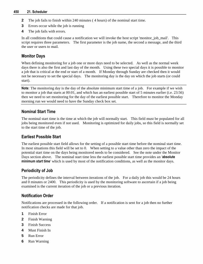
450 21. Scheduler
2 The job fails to finish within 240 minutes ( 4 hours) of the nominal start time.
3 Errors occur while the job is running
4 The job fails with errors.
In all conditions that could cause a notification we will invoke the host script 'monitor_job_mail'. This
script requires three parameters. The first parameter is the job name, the second a message, and the third
the user or users to mail.
Monitor Days
When defining monitoring for a job one or more days need to be selected. As well as the normal week
days there is also the first and last day of the month. Using these two special days it is possible to monitor
a job that is critical at the end or start of a month. If Monday through Sunday are checked then it would
not be necessary to set the special days. The monitoring day is the day on which the job starts (or could
start).
Note: The monitoring day is the day of the absolute minimum start time of a job. For example if we wish
to monitor a job that starts at 00:01, and which has an earliest possible start of 5 minutes earlier (i.e. 23:56)
then we need to set monitoring for the day of the earliest possible start. Therefore to monitor the Monday
morning run we would need to have the Sunday check box set.
Nominal Start Time
The nominal start time is the time at which the job will normally start. This field must be populated for all
jobs being monitored even if not used. Monitoring is optimized for daily jobs, so this field is normally set
to the start time of the job.
Earliest Possible Start
The earliest possible start field allows for the setting of a possible start time before the nominal start time.
In most situations this field will be set to 0. When setting to a value other than zero the impact of the
potential start time on the days being monitored needs to be considered. See the note under the Monitor
Days section above. The nominal start time less the earliest possible start time provides an 'absolute minimum start time' which is used by most of the notification conditions, as well as the monitor days.
Periodicity of Job
The periodicity defines the interval between iterations of the job. For a daily job this would be 24 hours
and 0 minutes or 2400. This periodicity is used by the monitoring software to ascertain if a job being
examined is the current iteration of the job or a previous iteration.
Notification Order
Notifications are processed in the following order. If a notification is sent for a job then no further
notification checks are made for that job.
1 Finish Error
2 Finish Warning
3 Finish Success
4 Must Finish In
5 Run Error
6 Run Warning

Chapter 21 21. Scheduler 451
7 Checkpoint 3
8 Checkpoint 2
9 Checkpoint 1
10 Must Start Within
452 21. Scheduler
To fully cover all possible events it is usually necessary to set multiple notifications.
Must Start Within (Notification)
The 'must start within' notification allows notification when a job fails to start within a specified number of
minutes of the absolute minimum start time. In the example dialog above the job must start within 60
minutes of the start time.
If this criteria is not met then the monitoring software will look at the 'Action script' and 'Parameter to
script' fields to ascertain how to process the notification. If an action script has been defined then this
script will be executed in the Unix environment and will be passed the defined parameters. If no script is
defined then the 'Parameter to script' field will be executed in the Unix environment.
An example notification script is included as a template called 'unix_mon_job_mail'.
Must Finish In (Notification)
The 'must finish in' notification allows notification when a job fails to finish within a specified number of
minutes of the absolute minimum start time. In the example dialog above the job must finish within 4
hours of the start time. See the notes under 'Must Start Within' for the action taken if the criteria is met.
Run Warning Count (Notification)
The 'run warning count' notification allows notification when a job exceeds a specified number of warning
messages whilst running. This notification will only occur when a job is running. If the job has failed to
start, has finished or failed before the external monitor checks the number of warnings this notification will
be ignored. See the notes under 'Must Start Within' for the action taken if the criteria is met.
Run Error Count (Notification)
The 'run error count' notification allows notification when a job exceeds a specified number of error
messages whilst running. This notification will only occur when a job is running. If the job has failed to
start, has finished or failed before the external monitor checks the number of errors this notification will be
ignored. See the notes under 'Must Start Within' for the action taken if the criteria is met.
Finish Warning Count (Notification)
The 'finish warning count' notification allows notification when a job has exceeded a specified number of
warning messages and has completed or failed. This notification will only occur when a job has completed
or failed. If the job has failed to start or is still running when the external monitor checks the number of
warnings this notification will be ignored. See the notes under 'Must Start Within' for the action taken if
the criteria is met.
Finish Error Count (Notification)
The 'finish error count' notification allows notification when a job has exceeded a specified number of error
messages and has failed. This notification will only occur when a job has failed. If the job is still running
when the external monitor checks the number of warnings, this notification will be ignored. If the job has
been restarted and gone on to complete normally, this notification will be ignored even when errors have
occurred. See the notes under 'Must Start Within' for the action taken if the criteria is met.
Finish Success (Notification)
Chapter 21 21. Scheduler 453
The 'finish success' notification allows notification when a job completes. This notification can be used for
example to mail a log of the completed job to a specified user. See the notes under 'Must Start Within' for
the action taken if the criteria is met.
Checkpoint 1 (Notification)
The 'checkpoint 1' notification allows notification when a job fails to achieve either a specified number of
task completions, or a specified number of information/OK messages within a specified elapsed time. The
elapsed time is the time from the absolute minimum start time. This notification will only occur when the
job is running. If the job has failed to start, completed or failed when the external monitor checks the
checkpoint, this notification will be ignored. See the notes under 'Must Start Within' for the action taken if
the criteria is not met.
Checkpoint 2 (Notification)
The 'checkpoint 2' notification allows notification when a job fails to achieve either a specified number of
task completions, or a specified number of information/OK messages within a specified elapsed time. The
elapsed time is the time from the absolute minimum start time. This notification will only occur when the
job is running. If the job has failed to start, completed or failed when the external monitor checks the
checkpoint, this notification will be ignored. See the notes under 'Must Start Within' for the action taken if
the criteria is not met.
Checkpoint 3 (Notification)
The 'checkpoint 3' notification allows notification when a job fails to achieve either a specified number of
task completions, or a specified number of information/OK messages within a specified elapsed time. The
elapsed time is the time from the absolute minimum start time. This notification will only occur when the
job is running. If the job has failed to start, completed or failed when the external monitor checks the
checkpoint, this notification will be ignored. See the notes under 'Must Start Within' for the action taken if
the criteria is not met.
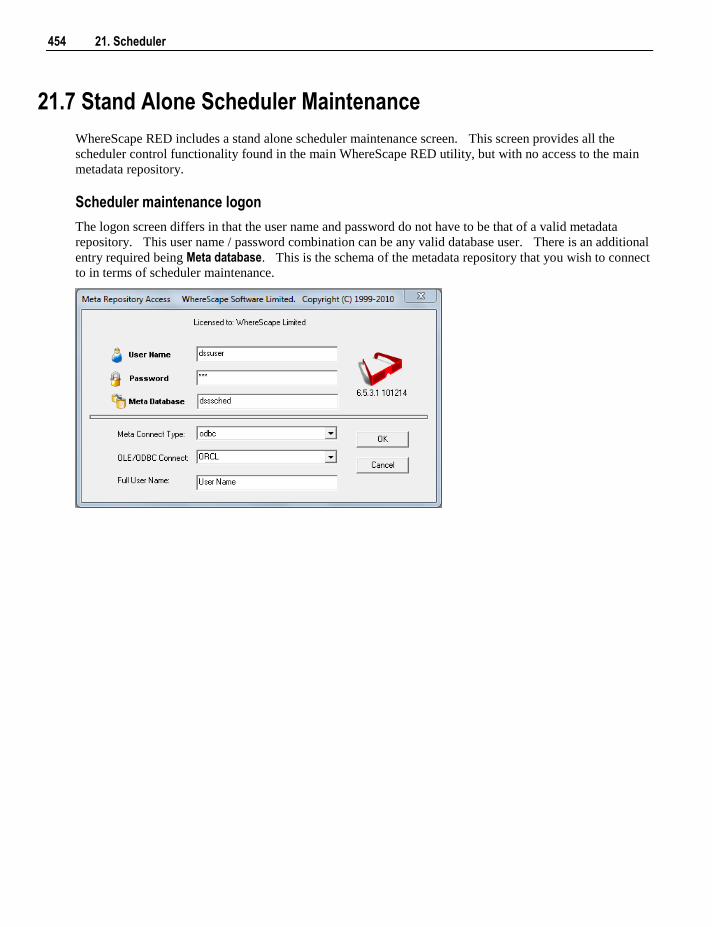
454 21. Scheduler
21.7 Stand Alone Scheduler Maintenance
WhereScape RED includes a stand alone scheduler maintenance screen. This screen provides all the
scheduler control functionality found in the main WhereScape RED utility, but with no access to the main
metadata repository.
Scheduler maintenance logon
The logon screen differs in that the user name and password do not have to be that of a valid metadata
repository. This user name / password combination can be any valid database user. There is an additional
entry required being Meta database. This is the schema of the metadata repository that you wish to connect
to in terms of scheduler maintenance.
Chapter 21 21. Scheduler 455
For SQL Server the Meta database must be set to dbo.
For Oracle data warehouses the 'Meta database' owner must have made the following grants to the specified
user before the scheduler maintenance utility can be used.
Scheduler maintenance grants
Repository access grants:
grant select on ws_meta to dsssched;
grant select on ws_meta_tables to dsssched;
grant select on ws_obj_type to dsssched;
grant select,insert on ws_user_adm to dsssched;
grant select,insert,update on ws_user_adm to dsssched;
grant select,alter on ws_wrk_job_dependency_seq to dsssched;
Object access (job create) grants:
grant select on ws_obj_object to dsssched;
grant select on ws_obj_pro_map to dsssched;
grant select on ws_obj_project to dsssched;
grant select on ws_obj_group to dsssched;
grant select on ws_pro_gro_map to dsssched;
Scheduler status grants:
grant select on ws_wrk_audit_log to dsssched;
Scheduler status, and job deletion grants:
grant select,delete on ws_wrk_error_log to dsssched;
Scheduler status, poll grants:
grant select,update on ws_wrk_scheduler to dsssched;
Job creation grants:
grant select,insert,update,delete on ws_wrk_dependency to dsssched;
grant select,insert,update,delete on ws_wrk_job_ctrl to dsssched;
grant select,alter on ws_job_seq to dsssched;
grant select,alter on ws_task_seq to dsssched;
Job maintenance grants:
grant select,insert,delete on ws_wrk_job_log to dsssched;
grant select,update,delete on ws_wrk_job_run to dsssched;
grant select,insert,update,delete on ws_wrk_dependency to dsssched;
grant select,insert,update,delete on ws_wrk_job_dependency to dsssched;
grant select,delete on ws_wrk_job_thread to dsssched;
Task maintenance grants:
grant select,insert,update,delete on ws_wrk_task_ctrl to dsssched;
grant select,update,delete on ws_wrk_task_run to dsssched;
grant select,insert,delete on ws_wrk_task_log to dsssched;
456 21. Scheduler
grant select,insert,update on dss_parameter to dsssched;
Right mouse 'used by' option in parameters listing grants:
grant select on ws_pro_header to dsssched;
grant select on ws_pro_line to dsssched;
grant select on ws_scr_header to dsssched;
grant select on ws_scr_line to dsssched;
grant select on ws_load_tab to dsssched;
grant select on ws_load_col to dsssched;
grant select on ws_stage_tab to dsssched;
grant select on ws_stage_col to dsssched;
grant select on ws_dim_tab to dsssched;
grant select on ws_dim_col to dsssched;
grant select on ws_fact_tab to dsssched;
grant select on ws_fact_col to dsssched;
grant select on ws_agg_tab to dsssched;
grant select on ws_agg_col to dsssched;
A sample script to grant these privileges is shipped with WhereScape RED. This script is called
'grant_sched_access.sql' and can be found in the WhereScape program directory.
The scheduler maintenance utility does not require a WhereScape license key. The WhereScape RED
software can be installed onto a PC, and this utility utilized without having to use the WhereScape 'Setup
Administrator' utility.
Chapter 22 22. Indexes 457
Indexes may exist on any table defined in WhereScape RED. By default WhereScape RED will
auto-generate a number of indexes during the drag and drop process and when building procedures. These
indexes can be altered or deleted. New indexes can be created as desired.
Note: The maintenance of the indexes is performed as part of the normal scheduler processing.
In the left pane right click on a table to:
Display indexes
Add indexes
In This Chapter
22.1 Index Definition .................................................................. 458
22.2 Index Storage Properties ..................................................... 464
22.3 Index Menu Options ............................................................ 468
C H A P T E R 2 2
22. Indexes
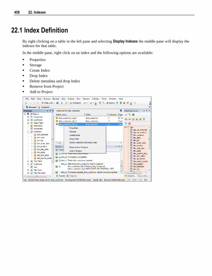
458 22. Indexes
22.1 Index Definition
By right clicking on a table in the left pane and selecting Display Indexes the middle pane will display the
indexes for that table.
In the middle pane, right click on an index and the following options are available:
Properties
Storage
Create Index
Drop Index
Delete metadata and drop Index
Remove from Project
Add to Project
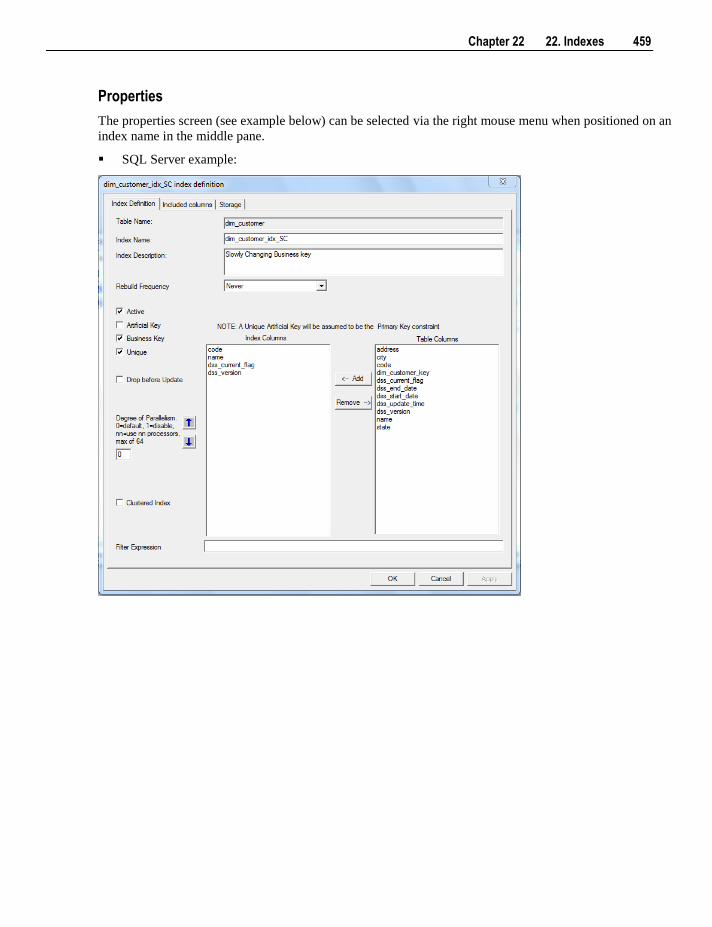
Chapter 22 22. Indexes 459
Properties
The properties screen (see example below) can be selected via the right mouse menu when positioned on an
index name in the middle pane.
SQL Server example:
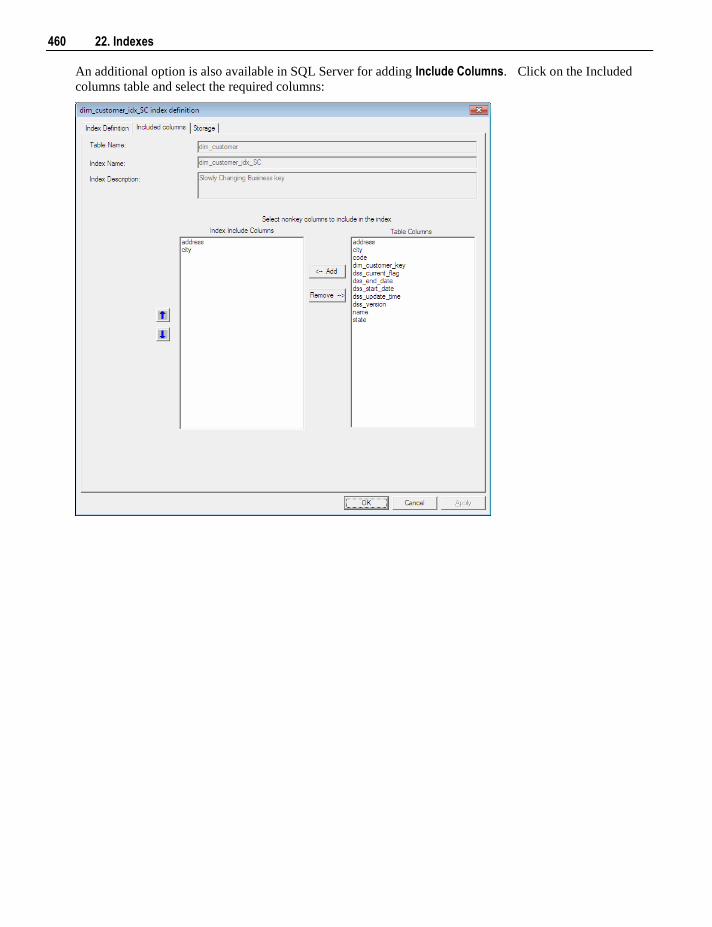
460 22. Indexes
An additional option is also available in SQL Server for adding Include Columns. Click on the Included
columns table and select the required columns:
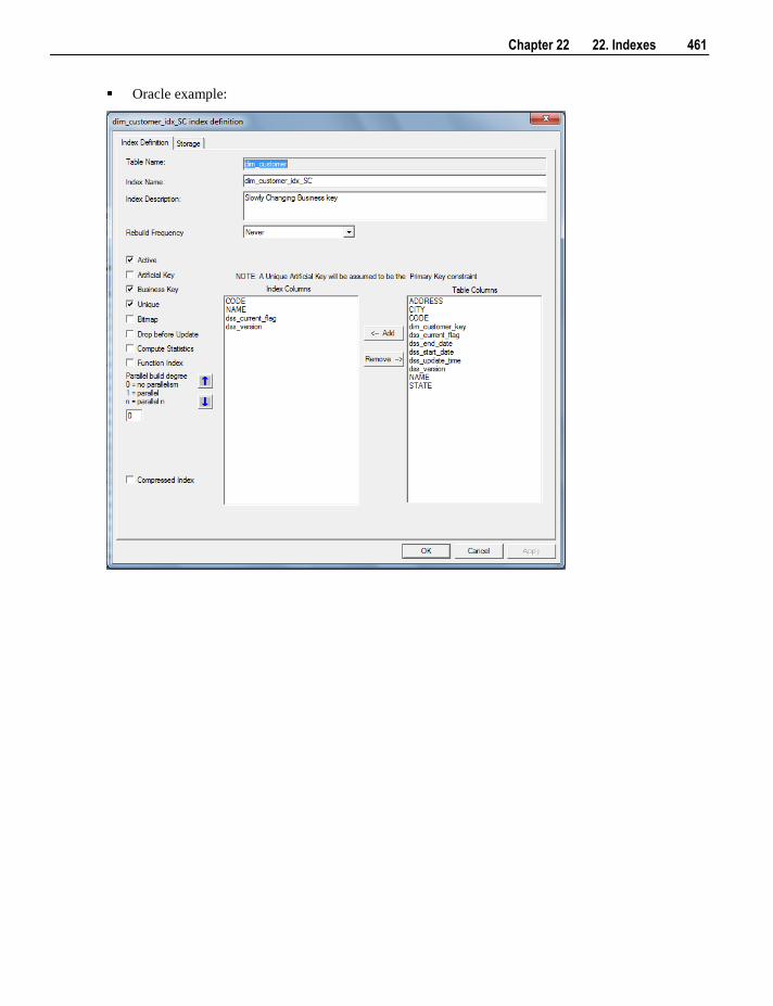
Chapter 22 22. Indexes 461
Oracle example:
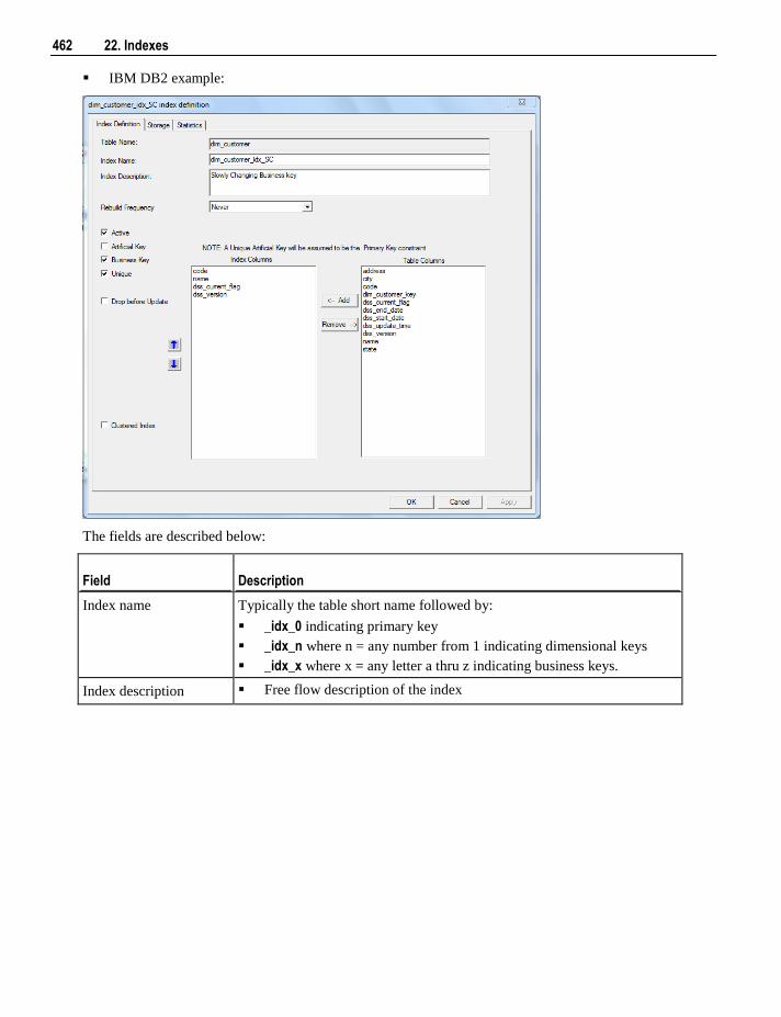
462 22. Indexes
IBM DB2 example:
The fields are described below:
Field Description
Index name Typically the table short name followed by:
_idx_0 indicating primary key
_idx_n where n = any number from 1 indicating dimensional keys
_idx_x where x = any letter a thru z indicating business keys.
Index description Free flow description of the index
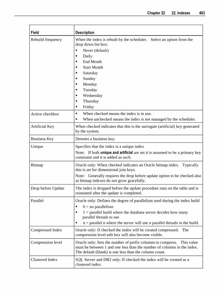
Chapter 22 22. Indexes 463
Field Description
Rebuild frequency When the index is rebuilt by the scheduler. Select an option from the
drop down list box:
Never (default)
Daily
End Month
Start Month
Saturday
Sunday
Monday
Tuesday
Wednesday
Thursday
Friday
Active checkbox When checked means the index is in use.
When unchecked means the index is not managed by the scheduler.
Artificial Key When checked indicates that this is the surrogate (artificial) key generated
by the system.
Business Key Denotes a business key.
Unique Specifies that the index is a unique index
Note: If both unique and artificial are set it is assumed to be a primary key
constraint and it is added as such.
Bitmap Oracle only: When checked indicates an Oracle bitmap index. Typically
this is set for dimensional join keys.
Note: Generally requires the drop before update option to be checked also
as bitmap indexes do not grow gracefully.
Drop before Update The index is dropped before the update procedure runs on the table and is
reinstated after the update is completed.
Parallel Oracle only: Defines the degree of parallelism used during the index build
0 = no parallelism
1 = parallel build where the database server decides how many
parallel threads to use
n = parallel n where the server will use n parallel threads in the build.
Compressed Index Oracle only: If checked the index will be created compressed. The
compression level edit box will also become visible.
Compression level Oracle only: Sets the number of prefix columns to compress. This value
must be between 1 and one less than the number of columns in the index.
The default (blank) is one less than the column count.
Clustered Index SQL Server and DB2 only: If checked the index will be created as a
clustered index.
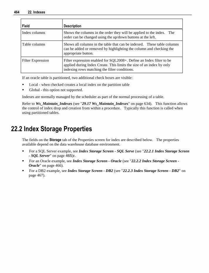
464 22. Indexes
Field Description
Index columns Shows the columns in the order they will be applied to the index. The
order can be changed using the up/down buttons at the left.
Table columns Shows all columns in the table that can be indexed. These table columns
can be added or removed by highlighting the column and checking the
appropriate button.
Filter Expression Filter expression enabled for SQL2008+. Define an Index filter to be
applied during Index Create. This limits the size of an index by only
indexing rows matching the filter conditions.
If an oracle table is partitioned, two additional check boxes are visible:
Local - when checked creates a local index on the partition table
Global - this option not supported.
Indexes are normally managed by the scheduler as part of the normal processing of a table.
Refer to Ws_Maintain_Indexes (see "29.17 Ws_Maintain_Indexes" on page 634). This function allows
the control of index drop and creation from within a procedure. Typically this function is called when
using partitioned tables.
22.2 Index Storage Properties
The fields on the Storage tab of the Properties screen for index are described below. The properties
available depend on the data warehouse database environment.
For a SQL Server example, see Index Storage Screen - SQL Serve (see "22.2.1 Index Storage Screen
- SQL Server" on page 465)r.
For an Oracle example, see Index Storage Screen - Oracle (see "22.2.2 Index Storage Screen -
Oracle" on page 466).
For a DB2 example, see Index Storage Screen - DB2 (see "22.2.3 Index Storage Screen - DB2" on
page 467).
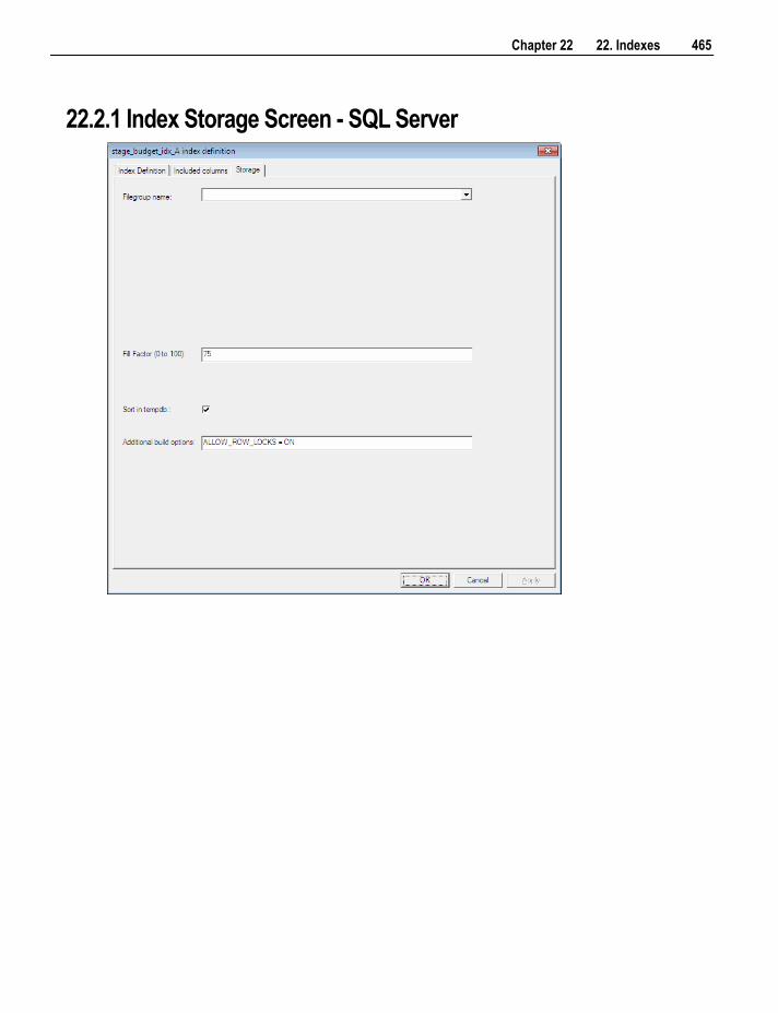
Chapter 22 22. Indexes 465
22.2.1 Index Storage Screen - SQL Server
466 22. Indexes
Filegroup name
Select a name from the drop down list box. If no filegroup name is selected for SQL Server, the default for
the database is used.
Fill Factor (0 to 100)
The amount of space to use in each leaf level page with creating or rebuilding the index. The default is 0 -
use the database default.
Note: This option is available from SQL Server 2005 onwards.
Sort in tempdb
If this check box is on WhereScape RED will tell SQL Server to use tempdb to store intermediate sort
results when creating or rebuilding the index. If this check box is off, WhereScape RED does not tell SQL
Server to use tempdb (so SQL Server uses the filegroup the index resides in). The default is off.
Note: This option is available from SQL Server 2005 onwards.
Additional build options
Enter any additional index creation options valid in SQL Server. The example above uses
ALLOW_ROW_LOCKS = ON, an option that enables the use of row locks when accessing the index.
22.2.2 Index Storage Screen - Oracle The storage properties for an Oracle index as the same as the storage properties for an Oracle table. Refer
to Table Storage Screen - Oracle (see "7.1.2 Table Storage Screen - Oracle" on page 109) for more
information.
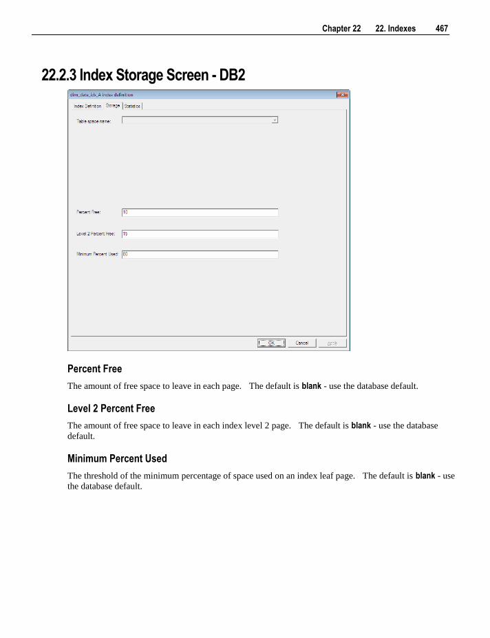
Chapter 22 22. Indexes 467
22.2.3 Index Storage Screen - DB2
Percent Free
The amount of free space to leave in each page. The default is blank - use the database default.
Level 2 Percent Free
The amount of free space to leave in each index level 2 page. The default is blank - use the database
default.
Minimum Percent Used
The threshold of the minimum percentage of space used on an index leaf page. The default is blank - use
the database default.
468 22. Indexes
22.3 Index Menu Options
The main Browser window has a menu section labelled 'Indexes'. Under this menu are a number of options
for dealing with indexes in bulk. Care should be taken when using these options, and an understanding of
what will occur is important.
Enable all foreign constraints
If an index has been defined as a foreign key constrain then this operation will enable the foreign constraint.
By default no auto generated indexes are created with foreign key constraints enabled.
Remove all foreign constraints
The index metadata is searched and any index that has a foreign key constraint enabled will have that
constraint removed from the database. On a large database this may be a very large operation.
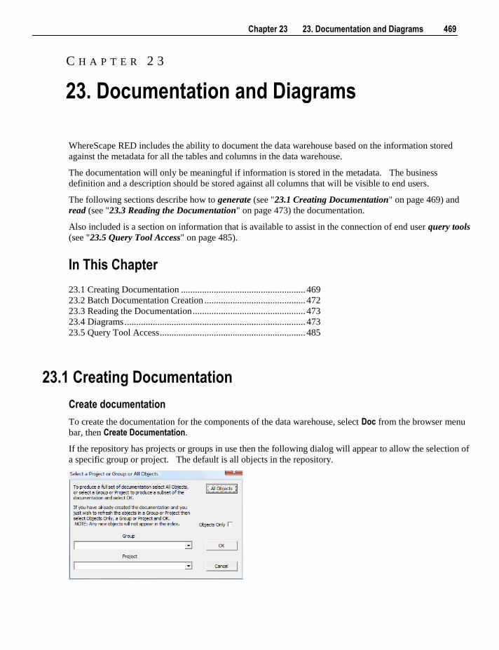
Chapter 23 23. Documentation and Diagrams 469
WhereScape RED includes the ability to document the data warehouse based on the information stored
against the metadata for all the tables and columns in the data warehouse.
The documentation will only be meaningful if information is stored in the metadata. The business
definition and a description should be stored against all columns that will be visible to end users.
The following sections describe how to generate (see "23.1 Creating Documentation" on page 469) and
read (see "23.3 Reading the Documentation" on page 473) the documentation.
Also included is a section on information that is available to assist in the connection of end user query tools
(see "23.5 Query Tool Access" on page 485).
In This Chapter
23.1 Creating Documentation ..................................................... 469
23.2 Batch Documentation Creation ........................................... 472
23.3 Reading the Documentation ................................................ 473
23.4 Diagrams ............................................................................. 473
23.5 Query Tool Access .............................................................. 485
23.1 Creating Documentation
Create documentation
To create the documentation for the components of the data warehouse, select Doc from the browser menu
bar, then Create Documentation.
If the repository has projects or groups in use then the following dialog will appear to allow the selection of
a specific group or project. The default is all objects in the repository.
C H A P T E R 2 3
23. Documentation and Diagrams

470 23. Documentation and Diagrams
A file dialog will appear next. Select a file path (directory) under which to save the HTML files that will
be produced.
A style sheet called mainstyle.css is created if it does not exist. If this style sheet exists then it is not
overwritten. The style sheet can therefore be modified to match an existing intranet standard.
The next screen allows for the inclusion of a banner and user defined links. It also provides some build
options:
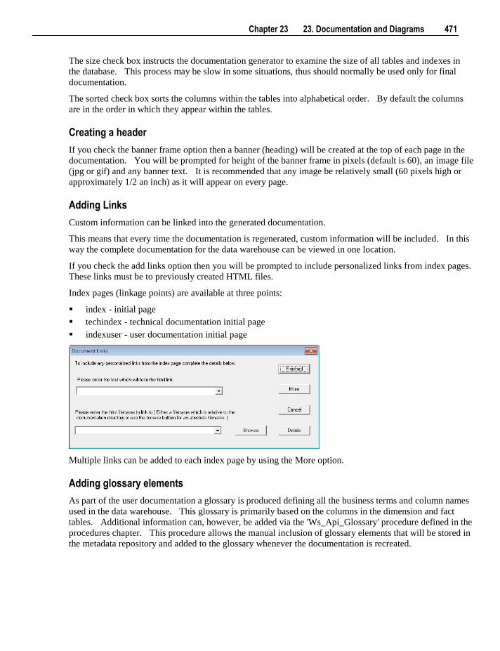
Chapter 23 23. Documentation and Diagrams 471
The size check box instructs the documentation generator to examine the size of all tables and indexes in
the database. This process may be slow in some situations, thus should normally be used only for final
documentation.
The sorted check box sorts the columns within the tables into alphabetical order. By default the columns
are in the order in which they appear within the tables.
Creating a header
If you check the banner frame option then a banner (heading) will be created at the top of each page in the
documentation. You will be prompted for height of the banner frame in pixels (default is 60), an image file
(jpg or gif) and any banner text. It is recommended that any image be relatively small (60 pixels high or
approximately 1/2 an inch) as it will appear on every page.
Adding Links
Custom information can be linked into the generated documentation.
This means that every time the documentation is regenerated, custom information will be included. In this
way the complete documentation for the data warehouse can be viewed in one location.
If you check the add links option then you will be prompted to include personalized links from index pages.
These links must be to previously created HTML files.
Index pages (linkage points) are available at three points:
index - initial page
techindex - technical documentation initial page
indexuser - user documentation initial page
Multiple links can be added to each index page by using the More option.
Adding glossary elements
As part of the user documentation a glossary is produced defining all the business terms and column names
used in the data warehouse. This glossary is primarily based on the columns in the dimension and fact
tables. Additional information can, however, be added via the 'Ws_Api_Glossary' procedure defined in the
procedures chapter. This procedure allows the manual inclusion of glossary elements that will be stored in
the metadata repository and added to the glossary whenever the documentation is recreated.
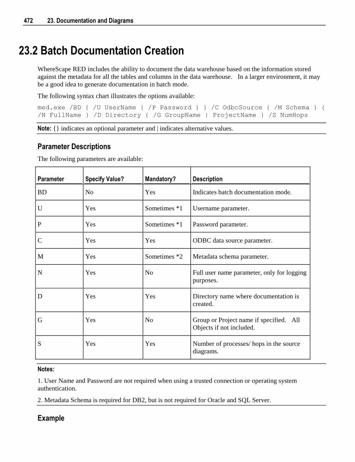
472 23. Documentation and Diagrams
23.2 Batch Documentation Creation
WhereScape RED includes the ability to document the data warehouse based on the information stored
against the metadata for all the tables and columns in the data warehouse. In a larger environment, it may
be a good idea to generate documentation in batch mode.
The following syntax chart illustrates the options available:
med.exe /BD { /U UserName { /P Password } } /C OdbcSource { /M Schema } {
/N FullName } /D Directory { /G GroupName | ProjectName } /S NumHops
Note: {} indicates an optional parameter and | indicates alternative values.
Parameter Descriptions
The following parameters are available:
Parameter Specify Value? Mandatory? Description
BD No Yes Indicates batch documentation mode.
U Yes Sometimes *1 Username parameter.
P Yes Sometimes *1 Password parameter.
C Yes Yes ODBC data source parameter.
M Yes Sometimes *2 Metadata schema parameter.
N Yes No Full user name parameter, only for logging
purposes.
D Yes Yes Directory name where documentation is
created.
G Yes No Group or Project name if specified. All
Objects if not included.
S Yes Yes Number of processes/ hops in the source
diagrams.
Notes:
1. User Name and Password are not required when using a trusted connection or operating system
authentication.
2. Metadata Schema is required for DB2, but is not required for Oracle and SQL Server.
Example
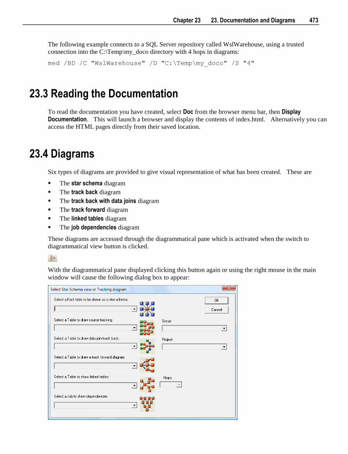
Chapter 23 23. Documentation and Diagrams 473
The following example connects to a SQL Server repository called WslWarehouse, using a trusted
connection into the C:\Temp\my_doco directory with 4 hops in diagrams:
med /BD /C "WslWarehouse" /D "C:\Temp\my_doco" /S "4"
23.3 Reading the Documentation
To read the documentation you have created, select Doc from the browser menu bar, then Display Documentation. This will launch a browser and display the contents of index.html. Alternatively you can
access the HTML pages directly from their saved location.
23.4 Diagrams
Six types of diagrams are provided to give visual representation of what has been created. These are
The star schema diagram
The track back diagram
The track back with data joins diagram
The track forward diagram
The linked tables diagram
The job dependencies diagram
These diagrams are accessed through the diagrammatical pane which is activated when the switch to
diagrammatical view button is clicked.
With the diagrammatical pane displayed clicking this button again or using the right mouse in the main
window will cause the following dialog box to appear:
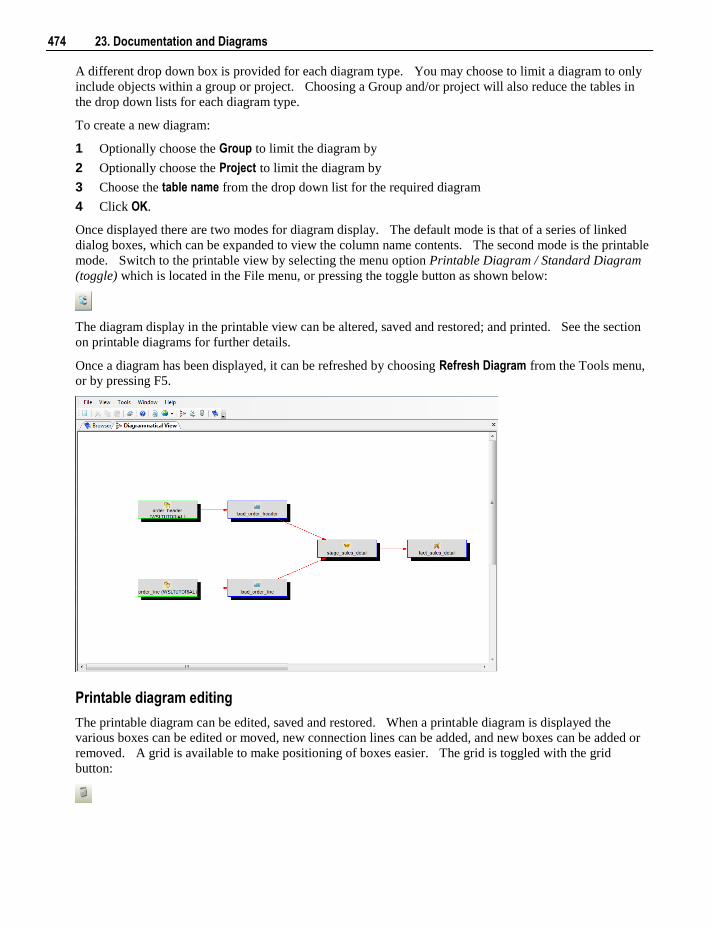
474 23. Documentation and Diagrams
A different drop down box is provided for each diagram type. You may choose to limit a diagram to only
include objects within a group or project. Choosing a Group and/or project will also reduce the tables in
the drop down lists for each diagram type.
To create a new diagram:
1 Optionally choose the Group to limit the diagram by
2 Optionally choose the Project to limit the diagram by
3 Choose the table name from the drop down list for the required diagram
4 Click OK.
Once displayed there are two modes for diagram display. The default mode is that of a series of linked
dialog boxes, which can be expanded to view the column name contents. The second mode is the printable
mode. Switch to the printable view by selecting the menu option Printable Diagram / Standard Diagram
(toggle) which is located in the File menu, or pressing the toggle button as shown below:
The diagram display in the printable view can be altered, saved and restored; and printed. See the section
on printable diagrams for further details.
Once a diagram has been displayed, it can be refreshed by choosing Refresh Diagram from the Tools menu,
or by pressing F5.
Printable diagram editing
The printable diagram can be edited, saved and restored. When a printable diagram is displayed the
various boxes can be edited or moved, new connection lines can be added, and new boxes can be added or
removed. A grid is available to make positioning of boxes easier. The grid is toggled with the grid
button:
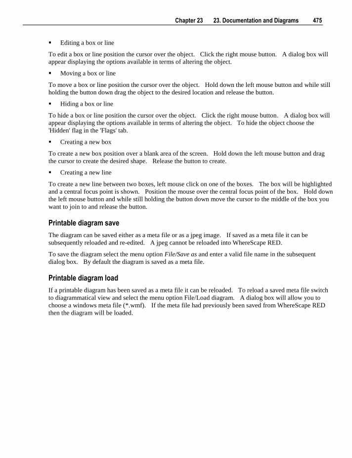
Chapter 23 23. Documentation and Diagrams 475
Editing a box or line
To edit a box or line position the cursor over the object. Click the right mouse button. A dialog box will
appear displaying the options available in terms of altering the object.
Moving a box or line
To move a box or line position the cursor over the object. Hold down the left mouse button and while still
holding the button down drag the object to the desired location and release the button.
Hiding a box or line
To hide a box or line position the cursor over the object. Click the right mouse button. A dialog box will
appear displaying the options available in terms of altering the object. To hide the object choose the
'Hidden' flag in the 'Flags' tab.
Creating a new box
To create a new box position over a blank area of the screen. Hold down the left mouse button and drag
the cursor to create the desired shape. Release the button to create.
Creating a new line
To create a new line between two boxes, left mouse click on one of the boxes. The box will be highlighted
and a central focus point is shown. Position the mouse over the central focus point of the box. Hold down
the left mouse button and while still holding the button down move the cursor to the middle of the box you
want to join to and release the button.
Printable diagram save
The diagram can be saved either as a meta file or as a jpeg image. If saved as a meta file it can be
subsequently reloaded and re-edited. A jpeg cannot be reloaded into WhereScape RED.
To save the diagram select the menu option File/Save as and enter a valid file name in the subsequent
dialog box. By default the diagram is saved as a meta file.
Printable diagram load
If a printable diagram has been saved as a meta file it can be reloaded. To reload a saved meta file switch
to diagrammatical view and select the menu option File/Load diagram. A dialog box will allow you to
choose a windows meta file (*.wmf). If the meta file had previously been saved from WhereScape RED
then the diagram will be loaded.
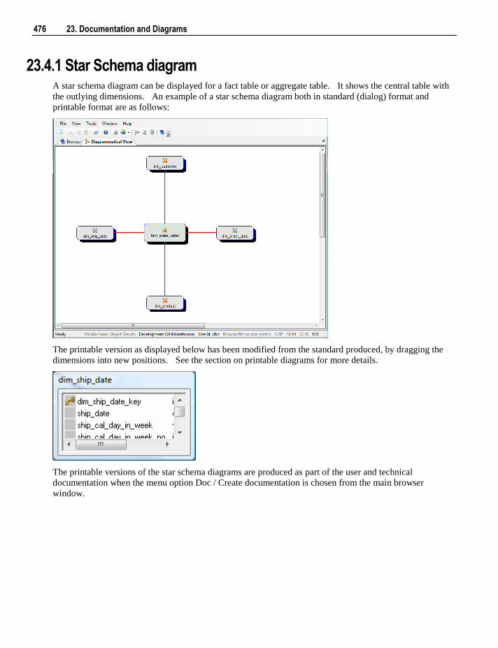
476 23. Documentation and Diagrams
23.4.1 Star Schema diagram A star schema diagram can be displayed for a fact table or aggregate table. It shows the central table with
the outlying dimensions. An example of a star schema diagram both in standard (dialog) format and
printable format are as follows:
The printable version as displayed below has been modified from the standard produced, by dragging the
dimensions into new positions. See the section on printable diagrams for more details.
The printable versions of the star schema diagrams are produced as part of the user and technical
documentation when the menu option Doc / Create documentation is chosen from the main browser
window.
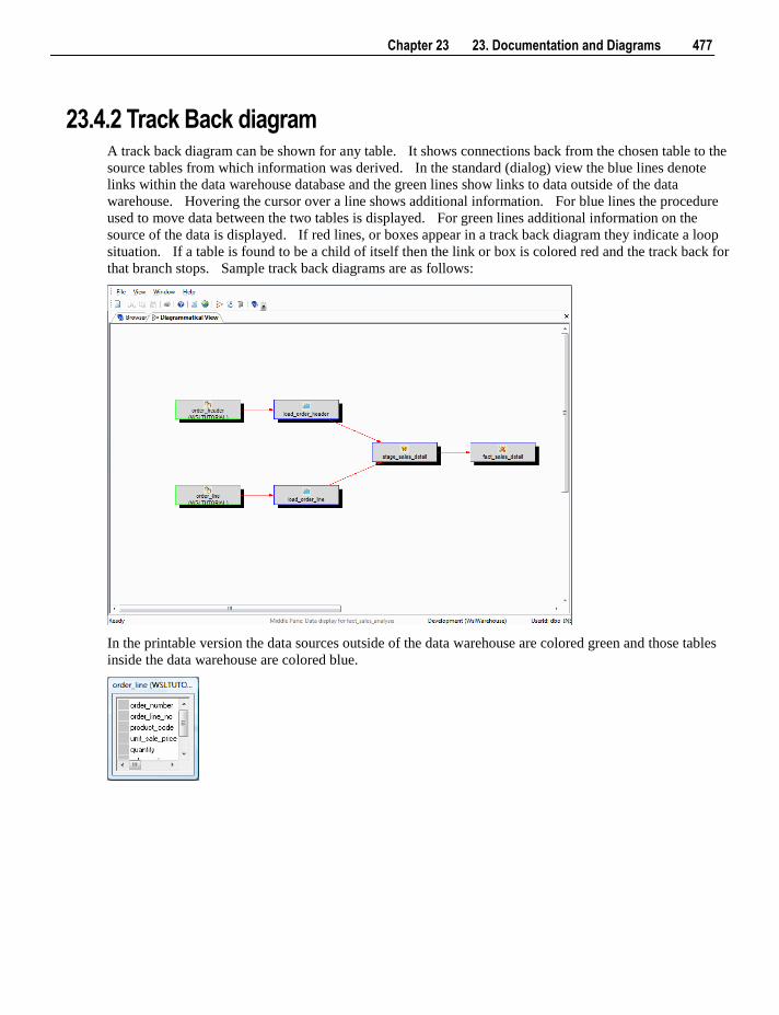
Chapter 23 23. Documentation and Diagrams 477
23.4.2 Track Back diagram A track back diagram can be shown for any table. It shows connections back from the chosen table to the
source tables from which information was derived. In the standard (dialog) view the blue lines denote
links within the data warehouse database and the green lines show links to data outside of the data
warehouse. Hovering the cursor over a line shows additional information. For blue lines the procedure
used to move data between the two tables is displayed. For green lines additional information on the
source of the data is displayed. If red lines, or boxes appear in a track back diagram they indicate a loop
situation. If a table is found to be a child of itself then the link or box is colored red and the track back for
that branch stops. Sample track back diagrams are as follows:
In the printable version the data sources outside of the data warehouse are colored green and those tables
inside the data warehouse are colored blue.
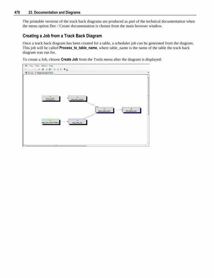
478 23. Documentation and Diagrams
The printable versions of the track back diagrams are produced as part of the technical documentation when
the menu option Doc / Create documentation is chosen from the main browser window.
Creating a Job from a Track Back Diagram
Once a track back diagram has been created for a table, a scheduler job can be generated from the diagram.
This job will be called Process_to_table_name, where table_name is the name of the table the track back
diagram was run for.
To create a Job, choose Create Job from the Tools menu after the diagram is displayed:
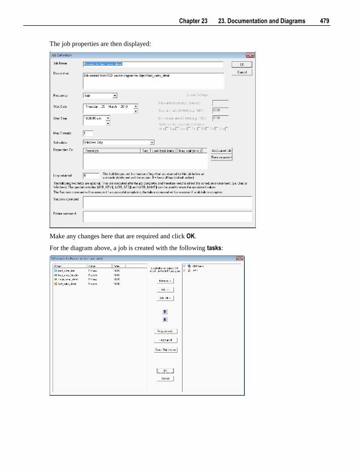
Chapter 23 23. Documentation and Diagrams 479
The job properties are then displayed:
Make any changes here that are required and click OK.
For the diagram above, a job is created with the following tasks:
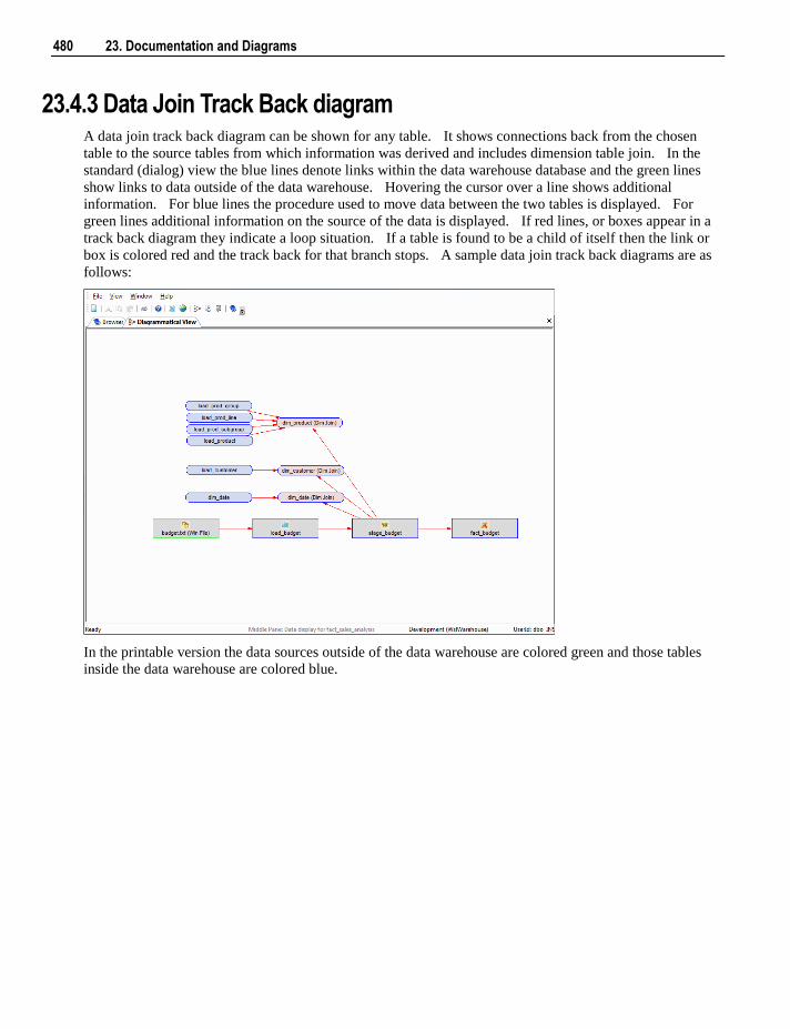
480 23. Documentation and Diagrams
23.4.3 Data Join Track Back diagram A data join track back diagram can be shown for any table. It shows connections back from the chosen
table to the source tables from which information was derived and includes dimension table join. In the
standard (dialog) view the blue lines denote links within the data warehouse database and the green lines
show links to data outside of the data warehouse. Hovering the cursor over a line shows additional
information. For blue lines the procedure used to move data between the two tables is displayed. For
green lines additional information on the source of the data is displayed. If red lines, or boxes appear in a
track back diagram they indicate a loop situation. If a table is found to be a child of itself then the link or
box is colored red and the track back for that branch stops. A sample data join track back diagrams are as
follows:
In the printable version the data sources outside of the data warehouse are colored green and those tables
inside the data warehouse are colored blue.
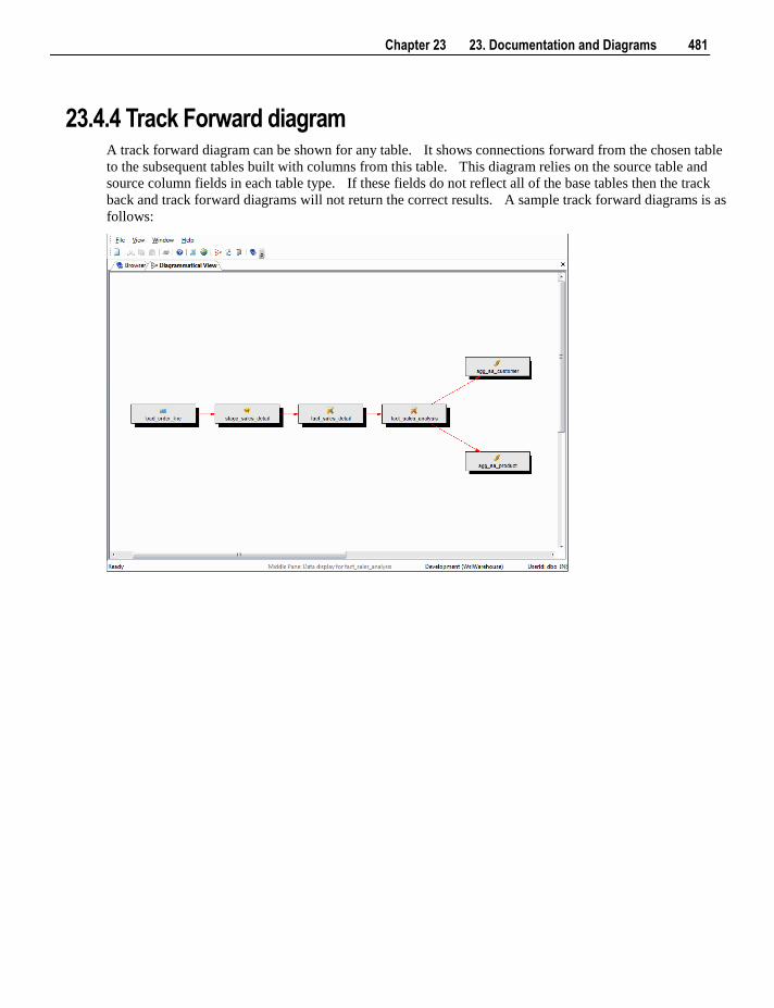
Chapter 23 23. Documentation and Diagrams 481
23.4.4 Track Forward diagram A track forward diagram can be shown for any table. It shows connections forward from the chosen table
to the subsequent tables built with columns from this table. This diagram relies on the source table and
source column fields in each table type. If these fields do not reflect all of the base tables then the track
back and track forward diagrams will not return the correct results. A sample track forward diagrams is as
follows:
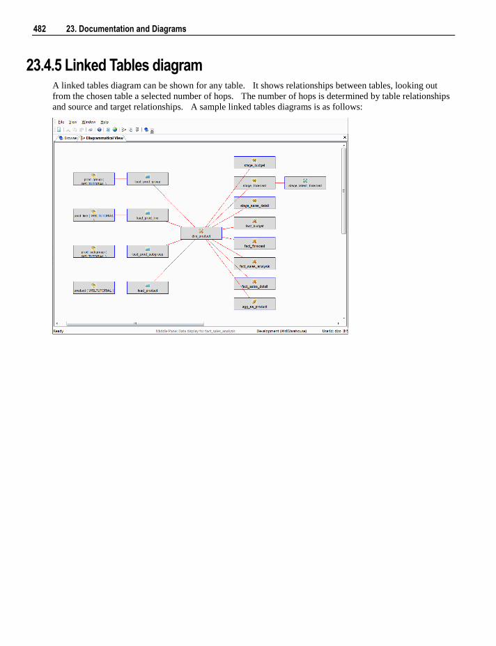
482 23. Documentation and Diagrams
23.4.5 Linked Tables diagram A linked tables diagram can be shown for any table. It shows relationships between tables, looking out
from the chosen table a selected number of hops. The number of hops is determined by table relationships
and source and target relationships. A sample linked tables diagrams is as follows:
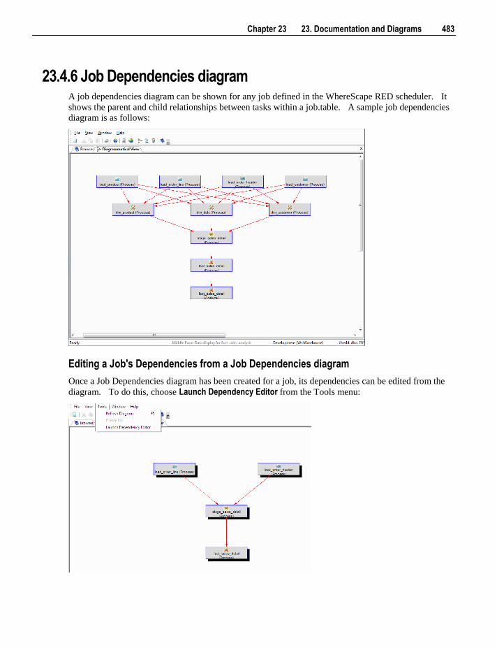
Chapter 23 23. Documentation and Diagrams 483
23.4.6 Job Dependencies diagram A job dependencies diagram can be shown for any job defined in the WhereScape RED scheduler. It
shows the parent and child relationships between tasks within a job.table. A sample job dependencies
diagram is as follows:
Editing a Job's Dependencies from a Job Dependencies diagram
Once a Job Dependencies diagram has been created for a job, its dependencies can be edited from the
diagram. To do this, choose Launch Dependency Editor from the Tools menu:
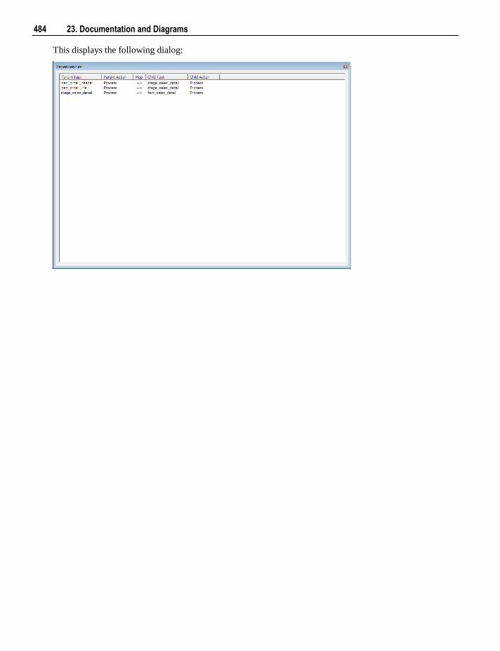
484 23. Documentation and Diagrams
This displays the following dialog:
Chapter 23 23. Documentation and Diagrams 485
23.5 Query Tool Access
Where the business definition has been set in the properties of either a fact or dimension column
WhereScape RED will attempt to record this information in the database. For the Oracle database this
business definition is stored as a column comment. Many end user query tools can make use of these
Oracle column comments. They can also be examined via the Oracle database system views
all_col_comments and user_col_comments. For the SQL Server database the business definition is also
stored as a column comment via the sp_addextendedproperty procedure with a property name of
'Comment'.
In addition a number of metadata views exist to make the task of connecting an end user query tool to the
data warehouse simpler. Many end user tools can make use of external data to populate their
end-user-layer (eul) definitions. Using these views end user query tools can utilize WhereScape RED's
business metadata. The views supplied are:
Dimension tables and columns
The view ws_admin_v_dim_col provides a listing of all columns in all dimensions that have the 'Eul visible'
flag set. Included in the information provided is the business definition and description of the column as
defined within WhereScape RED.
Fact tables and columns
The view ws_admin_v_fact_col provides a listing of all columns in all fact tables that have the 'Eul visible'
flag set. Included in the information provided is the business definition and description of the column as
defined within WhereScape RED.
Fact - Dimension Joins
The view ws_admin_v_fact_join provides a listing of all fact tables and all the dimensions that each fact
table joins to. Both the fact table dimension key column and the dimension key column are included in the
view.

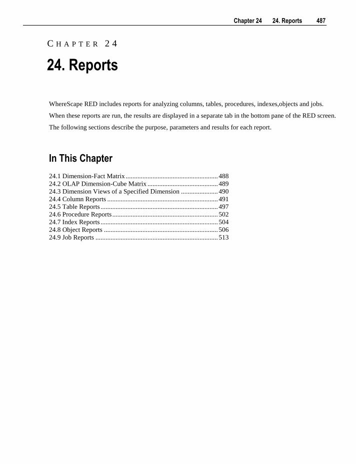
Chapter 24 24. Reports 487
WhereScape RED includes reports for analyzing columns, tables, procedures, indexes,objects and jobs.
When these reports are run, the results are displayed in a separate tab in the bottom pane of the RED screen.
The following sections describe the purpose, parameters and results for each report.
In This Chapter
24.1 Dimension-Fact Matrix ....................................................... 488
24.2 OLAP Dimension-Cube Matrix .......................................... 489
24.3 Dimension Views of a Specified Dimension ...................... 490
24.4 Column Reports .................................................................. 491
24.5 Table Reports ...................................................................... 497
24.6 Procedure Reports ............................................................... 502
24.7 Index Reports ...................................................................... 504
24.8 Object Reports .................................................................... 506
24.9 Job Reports ......................................................................... 513
C H A P T E R 2 4
24. Reports
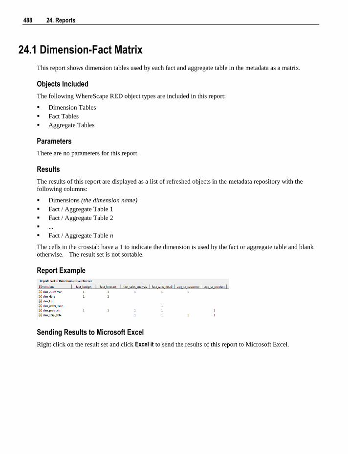
488 24. Reports
24.1 Dimension-Fact Matrix
This report shows dimension tables used by each fact and aggregate table in the metadata as a matrix.
Objects Included
The following WhereScape RED object types are included in this report:
Dimension Tables
Fact Tables
Aggregate Tables
Parameters
There are no parameters for this report.
Results
The results of this report are displayed as a list of refreshed objects in the metadata repository with the
following columns:
Dimensions (the dimension name)
Fact / Aggregate Table 1
Fact / Aggregate Table 2
...
Fact / Aggregate Table n
The cells in the crosstab have a 1 to indicate the dimension is used by the fact or aggregate table and blank
otherwise. The result set is not sortable.
Report Example
Sending Results to Microsoft Excel
Right click on the result set and click Excel it to send the results of this report to Microsoft Excel.
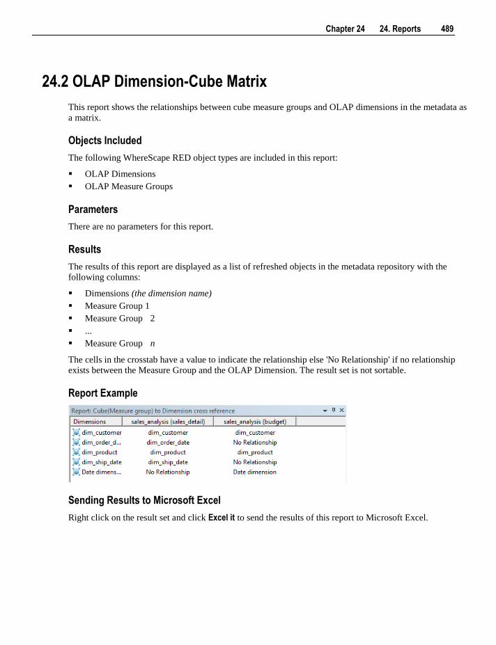
Chapter 24 24. Reports 489
24.2 OLAP Dimension-Cube Matrix
This report shows the relationships between cube measure groups and OLAP dimensions in the metadata as
a matrix.
Objects Included
The following WhereScape RED object types are included in this report:
OLAP Dimensions
OLAP Measure Groups
Parameters
There are no parameters for this report.
Results
The results of this report are displayed as a list of refreshed objects in the metadata repository with the
following columns:
Dimensions (the dimension name)
Measure Group 1
Measure Group 2
...
Measure Group n
The cells in the crosstab have a value to indicate the relationship else 'No Relationship' if no relationship
exists between the Measure Group and the OLAP Dimension. The result set is not sortable.
Report Example
Sending Results to Microsoft Excel
Right click on the result set and click Excel it to send the results of this report to Microsoft Excel.
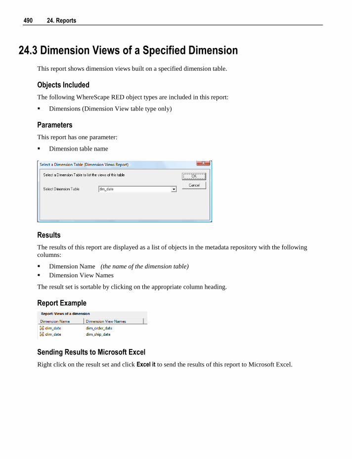
490 24. Reports
24.3 Dimension Views of a Specified Dimension
This report shows dimension views built on a specified dimension table.
Objects Included
The following WhereScape RED object types are included in this report:
Dimensions (Dimension View table type only)
Parameters
This report has one parameter:
Dimension table name
Results
The results of this report are displayed as a list of objects in the metadata repository with the following
columns:
Dimension Name (the name of the dimension table)
Dimension View Names
The result set is sortable by clicking on the appropriate column heading.
Report Example
Sending Results to Microsoft Excel
Right click on the result set and click Excel it to send the results of this report to Microsoft Excel.
Chapter 24 24. Reports 491
24.4 Column Reports
There are four reports for analyzing Columns:
Columns without Comments
All Column Transformations
Re-Usable Column Transformations
Column Track-Back
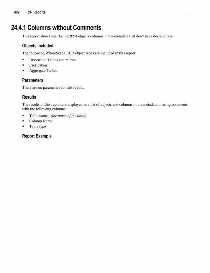
492 24. Reports
24.4.1 Columns without Comments This report shows user facing table objects columns in the metadata that don't have descriptions.
Objects Included
The following WhereScape RED object types are included in this report:
Dimension Tables and Views
Fact Tables
Aggregate Tables
Parameters
There are no parameters for this report.
Results
The results of this report are displayed as a list of objects and columns in the metadata missing comments
with the following columns:
Table name (the name of the table)
Column Name
Table type
Report Example
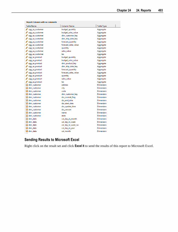
Chapter 24 24. Reports 493
Sending Results to Microsoft Excel
Right click on the result set and click Excel it to send the results of this report to Microsoft Excel.
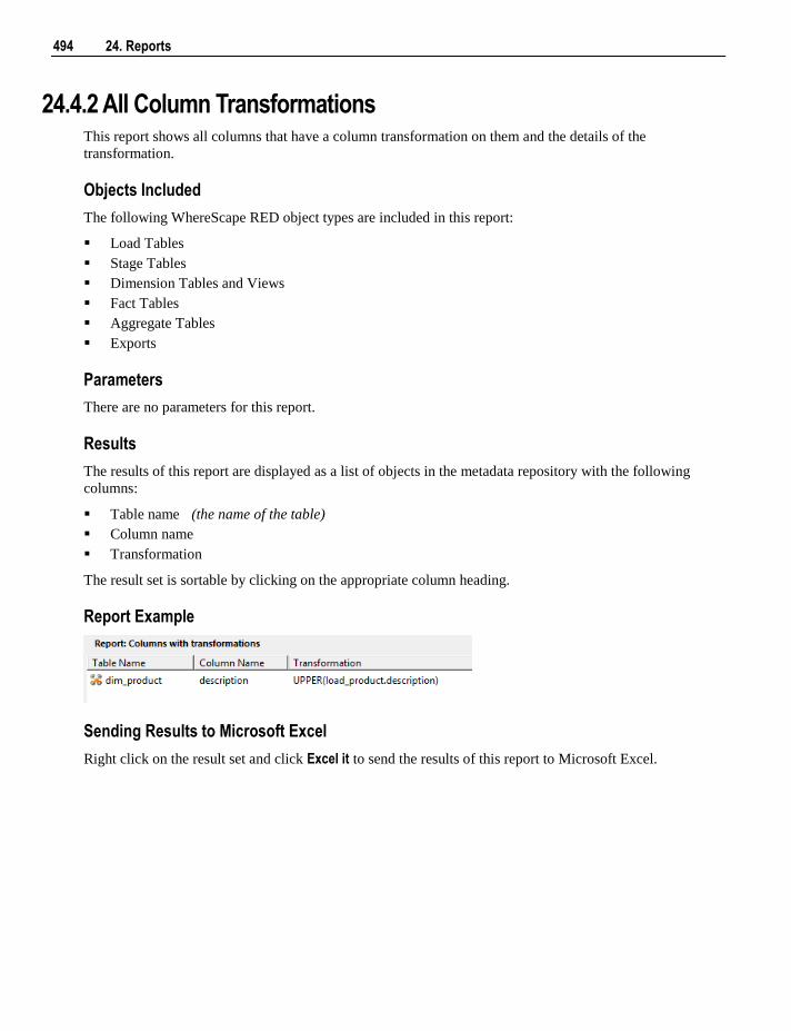
494 24. Reports
24.4.2 All Column Transformations This report shows all columns that have a column transformation on them and the details of the
transformation.
Objects Included
The following WhereScape RED object types are included in this report:
Load Tables
Stage Tables
Dimension Tables and Views
Fact Tables
Aggregate Tables
Exports
Parameters
There are no parameters for this report.
Results
The results of this report are displayed as a list of objects in the metadata repository with the following
columns:
Table name (the name of the table)
Column name
Transformation
The result set is sortable by clicking on the appropriate column heading.
Report Example
Sending Results to Microsoft Excel
Right click on the result set and click Excel it to send the results of this report to Microsoft Excel.
Chapter 24 24. Reports 495
24.4.3 Re-Usable Column Transformations This report shows all reusable transformations as defined via tools/Reusable transformations.
Parameters
There are no parameters for this report.
Results
The results of this report are displayed as a list of Re-Usable transformations with the following columns :
Template Name
Description
The result set is not sortable.
Report Example
Sending Results to Microsoft Excel
Right click on the result set and click Excel it to send the results of this report to Microsoft Excel.
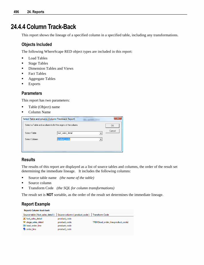
496 24. Reports
24.4.4 Column Track-Back This report shows the lineage of a specified column in a specified table, including any transformations.
Objects Included
The following WhereScape RED object types are included in this report:
Load Tables
Stage Tables
Dimension Tables and Views
Fact Tables
Aggregate Tables
Exports
Parameters
This report has two parameters:
Table (Object) name
Column Name
Results
The results of this report are displayed as a list of source tables and columns, the order of the result set
determining the immediate lineage. It includes the following columns:
Source table name (the name of the table)
Source column
Transform Code (the SQL for column transformations)
The result set is NOT sortable, as the order of the result set determines the immediate lineage.
Report Example
Chapter 24 24. Reports 497
Sending Results to Microsoft Excel
Right click on the result set and click Excel it to send the results of this report to Microsoft Excel.
24.5 Table Reports
There are four reports for analyzing Tables:
Tables without Comments
Load Tables by Connection
Records that failed a Dimension Join
External source table/files
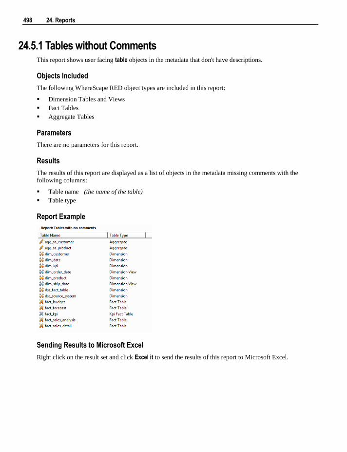
498 24. Reports
24.5.1 Tables without Comments This report shows user facing table objects in the metadata that don't have descriptions.
Objects Included
The following WhereScape RED object types are included in this report:
Dimension Tables and Views
Fact Tables
Aggregate Tables
Parameters
There are no parameters for this report.
Results
The results of this report are displayed as a list of objects in the metadata missing comments with the
following columns:
Table name (the name of the table)
Table type
Report Example
Sending Results to Microsoft Excel
Right click on the result set and click Excel it to send the results of this report to Microsoft Excel.
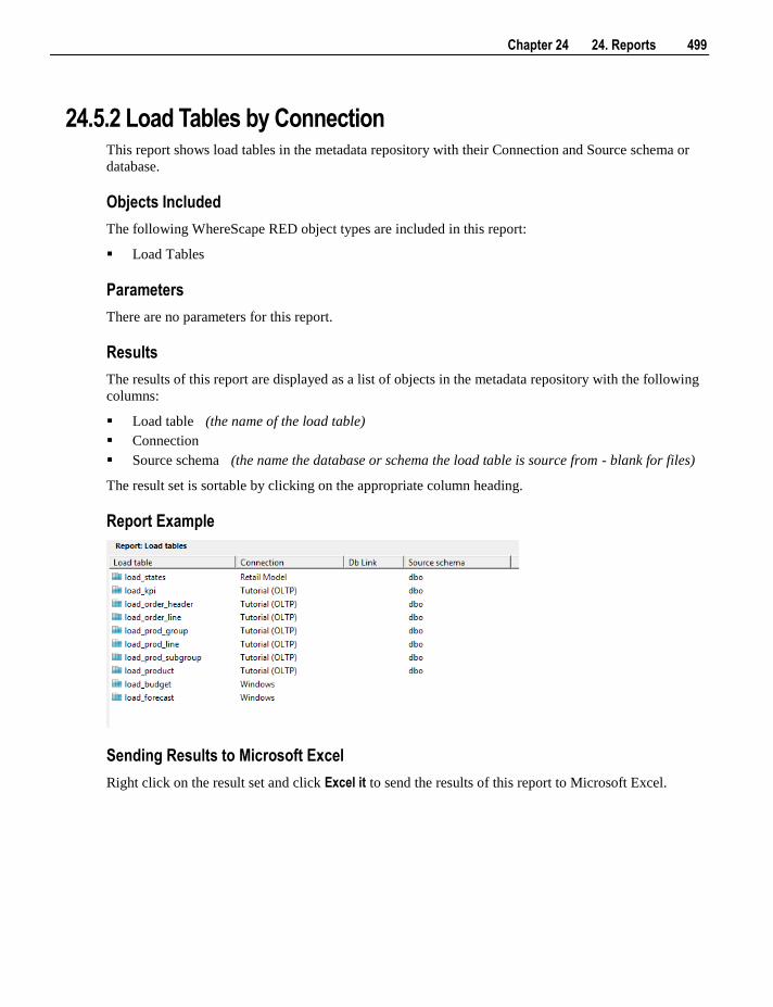
Chapter 24 24. Reports 499
24.5.2 Load Tables by Connection This report shows load tables in the metadata repository with their Connection and Source schema or
database.
Objects Included
The following WhereScape RED object types are included in this report:
Load Tables
Parameters
There are no parameters for this report.
Results
The results of this report are displayed as a list of objects in the metadata repository with the following
columns:
Load table (the name of the load table)
Connection
Source schema (the name the database or schema the load table is source from - blank for files)
The result set is sortable by clicking on the appropriate column heading.
Report Example
Sending Results to Microsoft Excel
Right click on the result set and click Excel it to send the results of this report to Microsoft Excel.
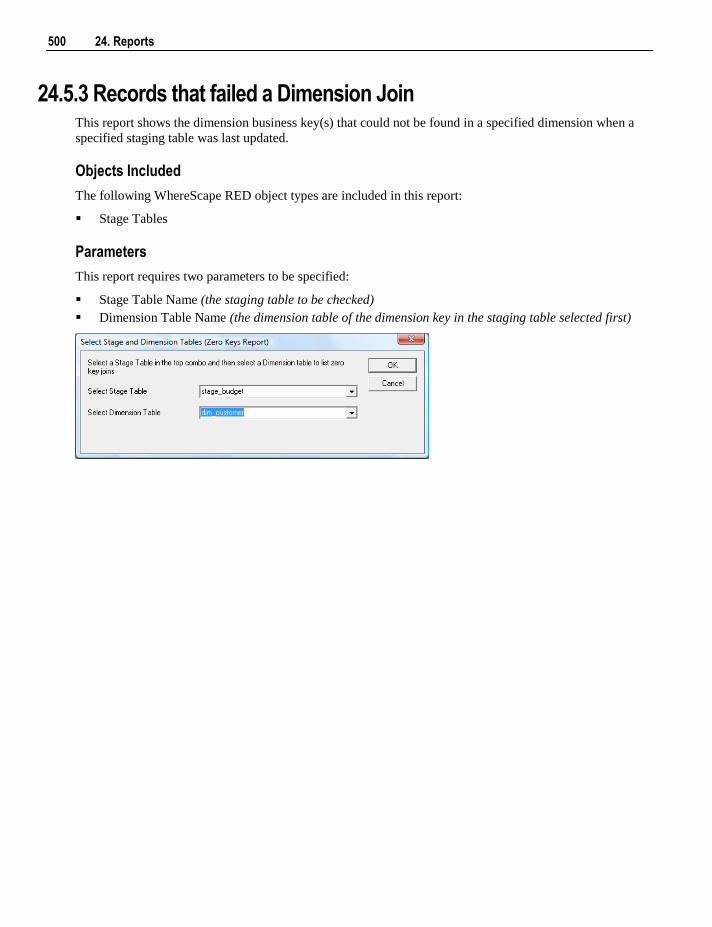
500 24. Reports
24.5.3 Records that failed a Dimension Join This report shows the dimension business key(s) that could not be found in a specified dimension when a
specified staging table was last updated.
Objects Included
The following WhereScape RED object types are included in this report:
Stage Tables
Parameters
This report requires two parameters to be specified:
Stage Table Name (the staging table to be checked)
Dimension Table Name (the dimension table of the dimension key in the staging table selected first)
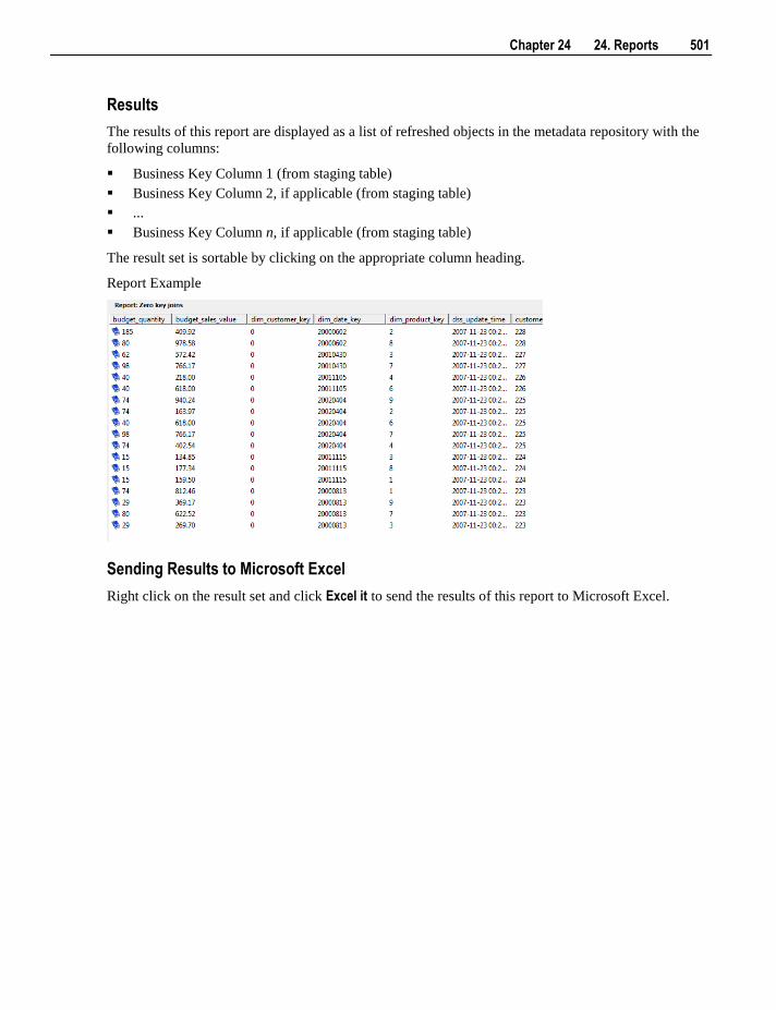
Chapter 24 24. Reports 501
Results
The results of this report are displayed as a list of refreshed objects in the metadata repository with the
following columns:
Business Key Column 1 (from staging table)
Business Key Column 2, if applicable (from staging table)
...
Business Key Column n, if applicable (from staging table)
The result set is sortable by clicking on the appropriate column heading.
Report Example
Sending Results to Microsoft Excel
Right click on the result set and click Excel it to send the results of this report to Microsoft Excel.
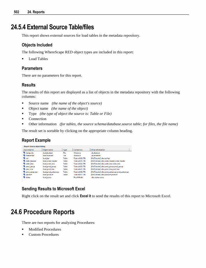
502 24. Reports
24.5.4 External Source Table/files This report shows external sources for load tables in the metadata repository.
Objects Included
The following WhereScape RED object types are included in this report:
Load Tables
Parameters
There are no parameters for this report.
Results
The results of this report are displayed as a list of objects in the metadata repository with the following
columns:
Source name (the name of the object's source)
Object name (the name of the object)
Type (the type of object the source is: Table or File)
Connection
Other information (for tables, the source schema/database.source table; for files, the file name)
The result set is sortable by clicking on the appropriate column heading.
Report Example
Sending Results to Microsoft Excel
Right click on the result set and click Excel it to send the results of this report to Microsoft Excel.
24.6 Procedure Reports
There are two reports for analyzing Procedures:
Modified Procedures
Custom Procedures
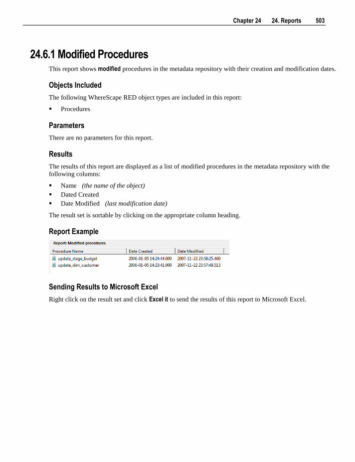
Chapter 24 24. Reports 503
24.6.1 Modified Procedures This report shows modified procedures in the metadata repository with their creation and modification dates.
Objects Included
The following WhereScape RED object types are included in this report:
Procedures
Parameters
There are no parameters for this report.
Results
The results of this report are displayed as a list of modified procedures in the metadata repository with the
following columns:
Name (the name of the object)
Dated Created
Date Modified (last modification date)
The result set is sortable by clicking on the appropriate column heading.
Report Example
Sending Results to Microsoft Excel
Right click on the result set and click Excel it to send the results of this report to Microsoft Excel.
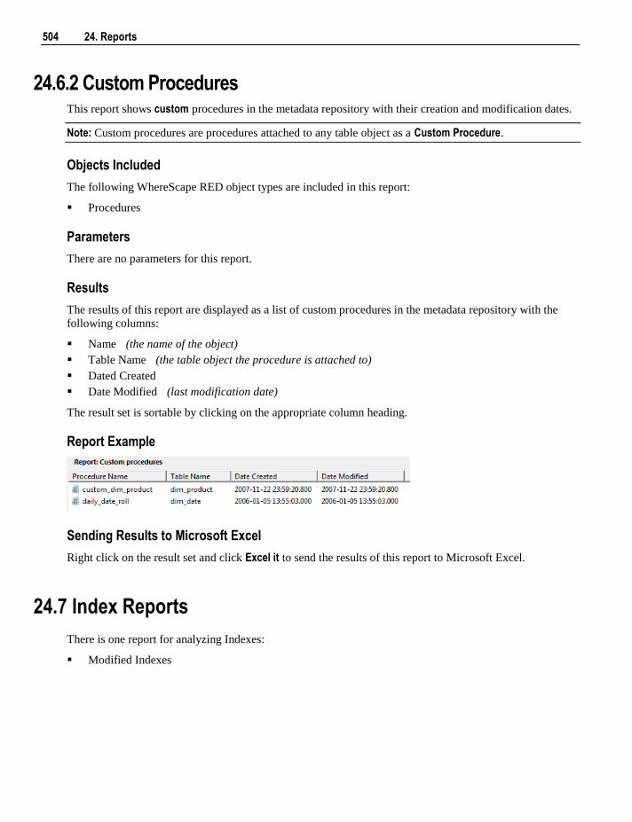
504 24. Reports
24.6.2 Custom Procedures This report shows custom procedures in the metadata repository with their creation and modification dates.
Note: Custom procedures are procedures attached to any table object as a Custom Procedure.
Objects Included
The following WhereScape RED object types are included in this report:
Procedures
Parameters
There are no parameters for this report.
Results
The results of this report are displayed as a list of custom procedures in the metadata repository with the
following columns:
Name (the name of the object)
Table Name (the table object the procedure is attached to)
Dated Created
Date Modified (last modification date)
The result set is sortable by clicking on the appropriate column heading.
Report Example
Sending Results to Microsoft Excel
Right click on the result set and click Excel it to send the results of this report to Microsoft Excel.
24.7 Index Reports
There is one report for analyzing Indexes:
Modified Indexes
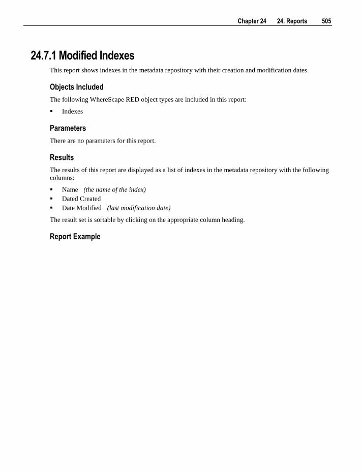
Chapter 24 24. Reports 505
24.7.1 Modified Indexes This report shows indexes in the metadata repository with their creation and modification dates.
Objects Included
The following WhereScape RED object types are included in this report:
Indexes
Parameters
There are no parameters for this report.
Results
The results of this report are displayed as a list of indexes in the metadata repository with the following
columns:
Name (the name of the index)
Dated Created
Date Modified (last modification date)
The result set is sortable by clicking on the appropriate column heading.
Report Example
506 24. Reports
Sending Results to Microsoft Excel
Right click on the result set and click Excel it to send the results of this report to Microsoft Excel.
24.8 Object Reports
There is four reports for analyzing Objects:
Objects-Project Matrix
Modified Objects (excluding indexes)
Objects Checked-out
Loaded or Imported Objects
Chapter 24 24. Reports 507
24.8.1 Objects-Project Matrix This report shows all objects that exist in one or more projects (other than All Objects) and the project(s) in
which they exist.
Objects Included
All object types are included in this report.
Parameters
There are no parameters for this report.
Results
The results of this report are displayed as a list of objects in the metadata repository that are in one or more
projects (other than All Objects) with the following columns as a grid:
Objects (the name of the object)
Project Name 1 (heading is the name of the first project, value is a 1 to indicate the object is in this
project, blank otherwise)
Project Name 2 (heading is the name of the second project, value is a 1 to indicate the object is in this
project, blank otherwise)
...
Project Name n (heading is the name of the nth project, value is a 1 to indicate the object is in this
project, blank otherwise)
The result set is sortable by clicking on the appropriate column heading.
Report Example
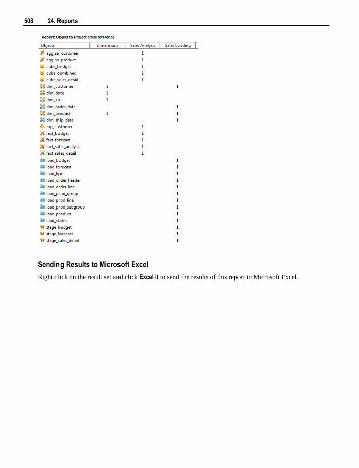
508 24. Reports
Sending Results to Microsoft Excel
Right click on the result set and click Excel it to send the results of this report to Microsoft Excel.
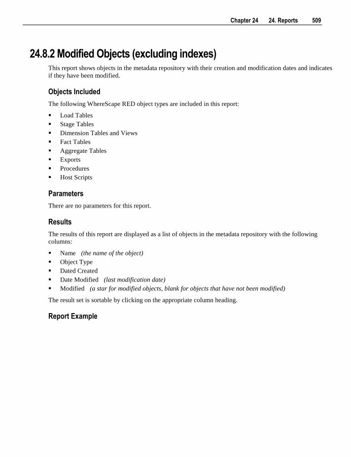
Chapter 24 24. Reports 509
24.8.2 Modified Objects (excluding indexes) This report shows objects in the metadata repository with their creation and modification dates and indicates
if they have been modified.
Objects Included
The following WhereScape RED object types are included in this report:
Load Tables
Stage Tables
Dimension Tables and Views
Fact Tables
Aggregate Tables
Exports
Procedures
Host Scripts
Parameters
There are no parameters for this report.
Results
The results of this report are displayed as a list of objects in the metadata repository with the following
columns:
Name (the name of the object)
Object Type
Dated Created
Date Modified (last modification date)
Modified (a star for modified objects, blank for objects that have not been modified)
The result set is sortable by clicking on the appropriate column heading.
Report Example
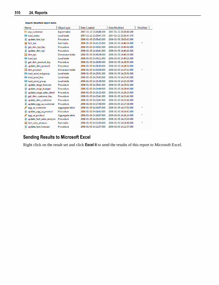
510 24. Reports
Sending Results to Microsoft Excel
Right click on the result set and click Excel it to send the results of this report to Microsoft Excel.
Chapter 24 24. Reports 511
24.8.3 Objects Checked-out This report lists all objects currently checked out.
Objects Included
All object types and data warehouse tables can be included in this report.
Parameters
There are no parameters for this report.
Results
The results of this report are displayed with the following columns:
Object Name (The name of the object)
Object Type (The type of the object, e.g. Fact, Dimension, etc)
Checked until (The date the object will be automatically checked back in)
Checked by (The name of the WhereScape RED user who checked out the object)
Reason (The reason provided for checking out the object)
Contact (The contact details provided when the object was checked out)
The result set is sortable by clicking on the appropriate column heading.
Report Example
Sending Results to Microsoft Excel
Right click on the result set and click Excel it to send the results of this report to Microsoft Excel.
512 24. Reports
24.8.4 Loaded or Imported Objects This report shows objects in the metadata repository that have been refreshed or imported from another
repository.
Objects Included
The following WhereScape RED object types are included in this report:
Load Tables
Stage Tables
Dimension Tables and Views
Fact Tables
Aggregate Tables
Join Indexes
Views
Cubes
Exports
Procedures
Host Scripts
Note: Indexes are not included.
Parameters
There are no parameters for this report.
Results
The results of this report are displayed as a list of refreshed objects in the metadata repository with the
following columns:
Object Name
Date (of last refresh or import)
Description (the kind of import or refresh)
Detail (not currently used)
The result set is sortable by clicking on the appropriate column heading.
Report Example
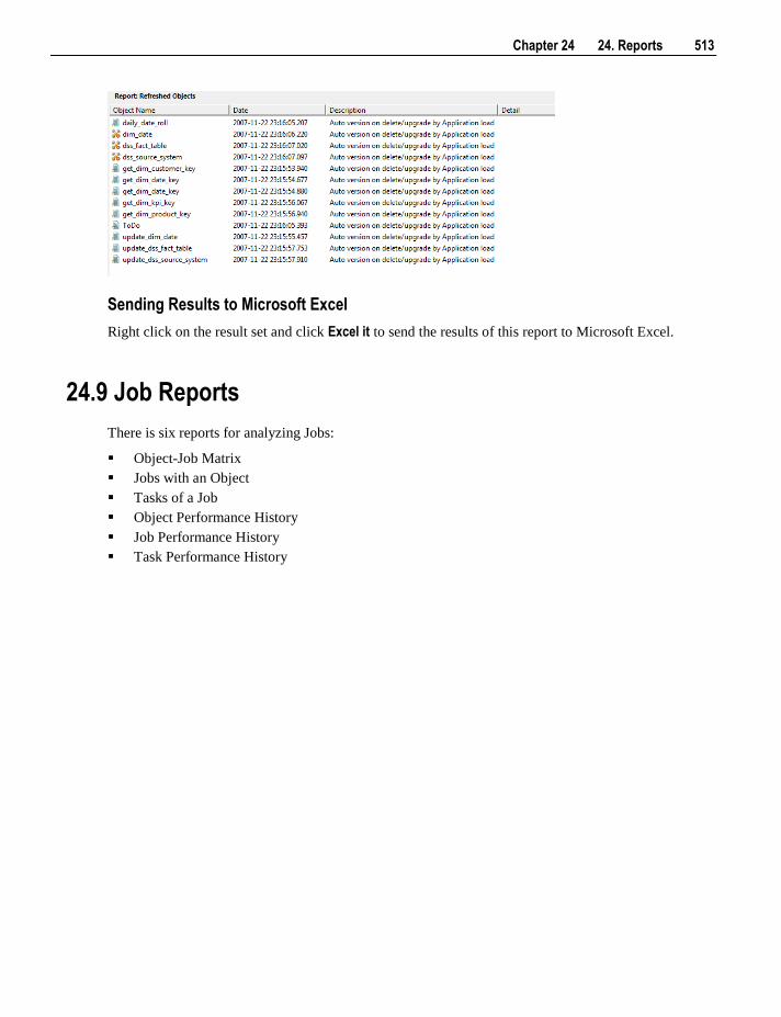
Chapter 24 24. Reports 513
Sending Results to Microsoft Excel
Right click on the result set and click Excel it to send the results of this report to Microsoft Excel.
24.9 Job Reports
There is six reports for analyzing Jobs:
Object-Job Matrix
Jobs with an Object
Tasks of a Job
Object Performance History
Job Performance History
Task Performance History
514 24. Reports
24.9.1 Object-Job Matrix This report shows all jobs and objects as well as the object actions. Table and Cube objects not in any jobs
also appears with No Job as their job.
Objects Included
All object types are included in this report.
Parameters
There are no parameters for this report.
Results
The results of this report are displayed as a list of jobs with the following columns:
Table Name (the name of the table or cube)
Action
Job Name (the name of the job)
Job Status
Job Last Run
Job Next Run
Report Example
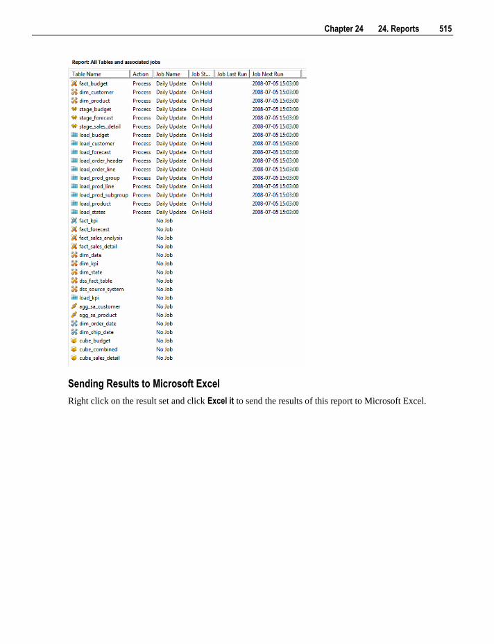
Chapter 24 24. Reports 515
Sending Results to Microsoft Excel
Right click on the result set and click Excel it to send the results of this report to Microsoft Excel.
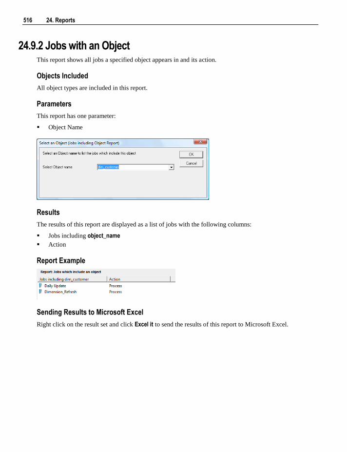
516 24. Reports
24.9.2 Jobs with an Object This report shows all jobs a specified object appears in and its action.
Objects Included
All object types are included in this report.
Parameters
This report has one parameter:
Object Name
Results
The results of this report are displayed as a list of jobs with the following columns:
Jobs including object_name
Action
Report Example
Sending Results to Microsoft Excel
Right click on the result set and click Excel it to send the results of this report to Microsoft Excel.
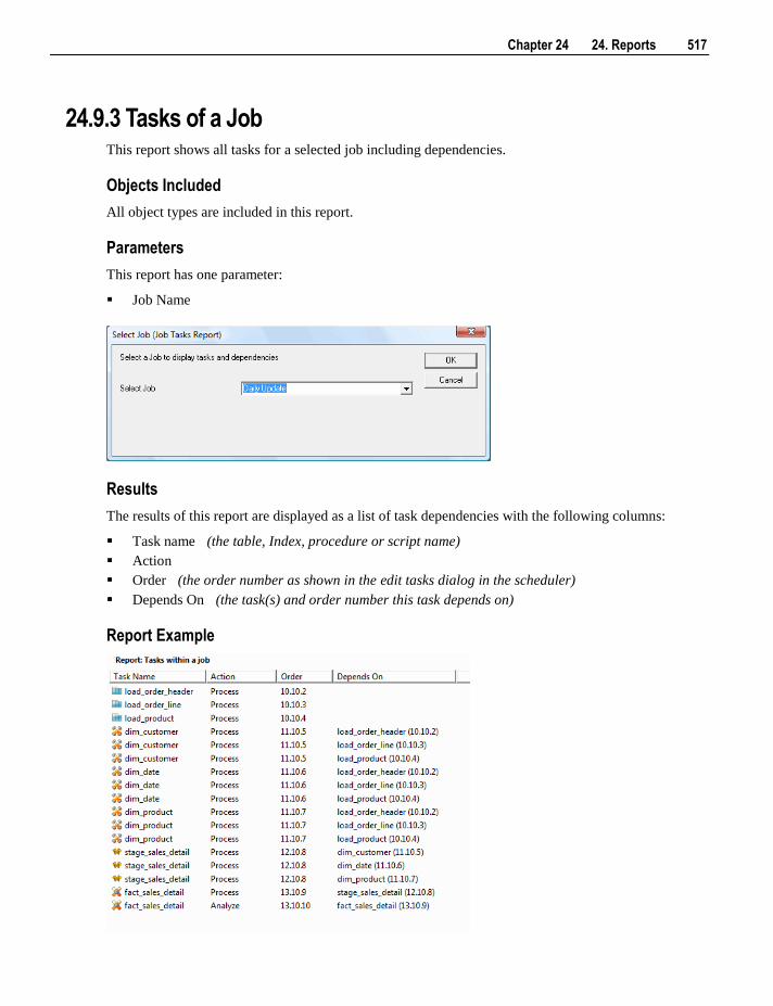
Chapter 24 24. Reports 517
24.9.3 Tasks of a Job This report shows all tasks for a selected job including dependencies.
Objects Included
All object types are included in this report.
Parameters
This report has one parameter:
Job Name
Results
The results of this report are displayed as a list of task dependencies with the following columns:
Task name (the table, Index, procedure or script name)
Action
Order (the order number as shown in the edit tasks dialog in the scheduler)
Depends On (the task(s) and order number this task depends on)
Report Example
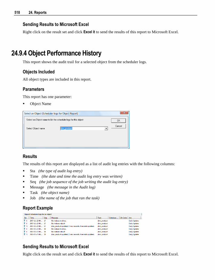
518 24. Reports
Sending Results to Microsoft Excel
Right click on the result set and click Excel it to send the results of this report to Microsoft Excel.
24.9.4 Object Performance History This report shows the audit trail for a selected object from the scheduler logs.
Objects Included
All object types are included in this report.
Parameters
This report has one parameter:
Object Name
Results
The results of this report are displayed as a list of audit log entries with the following columns:
Sta (the type of audit log entry)
Time (the date and time the audit log entry was written)
Seq (the job sequence of the job writing the audit log entry)
Message (the message in the Audit log)
Task (the object name)
Job (the name of the job that ran the task)
Report Example
Sending Results to Microsoft Excel
Right click on the result set and click Excel it to send the results of this report to Microsoft Excel.
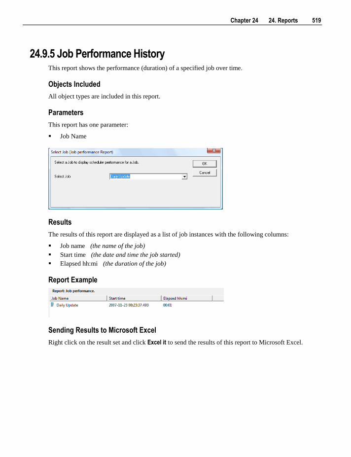
Chapter 24 24. Reports 519
24.9.5 Job Performance History This report shows the performance (duration) of a specified job over time.
Objects Included
All object types are included in this report.
Parameters
This report has one parameter:
Job Name
Results
The results of this report are displayed as a list of job instances with the following columns:
Job name (the name of the job)
Start time (the date and time the job started)
Elapsed hh:mi (the duration of the job)
Report Example
Sending Results to Microsoft Excel
Right click on the result set and click Excel it to send the results of this report to Microsoft Excel.
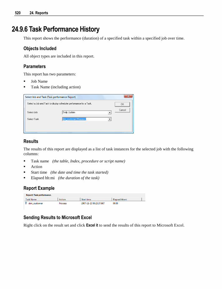
520 24. Reports
24.9.6 Task Performance History This report shows the performance (duration) of a specified task within a specified job over time.
Objects Included
All object types are included in this report.
Parameters
This report has two parameters:
Job Name
Task Name (including action)
Results
The results of this report are displayed as a list of task instances for the selected job with the following
columns:
Task name (the table, Index, procedure or script name)
Action
Start time (the date and time the task started)
Elapsed hh:mi (the duration of the task)
Report Example
Sending Results to Microsoft Excel
Right click on the result set and click Excel it to send the results of this report to Microsoft Excel.
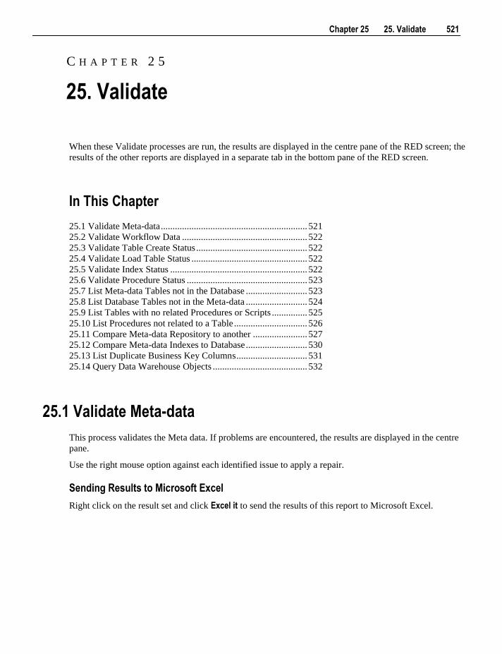
Chapter 25 25. Validate 521
When these Validate processes are run, the results are displayed in the centre pane of the RED screen; the
results of the other reports are displayed in a separate tab in the bottom pane of the RED screen.
In This Chapter
25.1 Validate Meta-data .............................................................. 521
25.2 Validate Workflow Data ..................................................... 522
25.3 Validate Table Create Status ............................................... 522
25.4 Validate Load Table Status ................................................. 522
25.5 Validate Index Status .......................................................... 522
25.6 Validate Procedure Status ................................................... 523
25.7 List Meta-data Tables not in the Database .......................... 523
25.8 List Database Tables not in the Meta-data .......................... 524
25.9 List Tables with no related Procedures or Scripts ............... 525
25.10 List Procedures not related to a Table ............................... 526
25.11 Compare Meta-data Repository to another ....................... 527
25.12 Compare Meta-data Indexes to Database .......................... 530
25.13 List Duplicate Business Key Columns .............................. 531
25.14 Query Data Warehouse Objects ........................................ 532
25.1 Validate Meta-data
This process validates the Meta data. If problems are encountered, the results are displayed in the centre
pane.
Use the right mouse option against each identified issue to apply a repair.
Sending Results to Microsoft Excel
Right click on the result set and click Excel it to send the results of this report to Microsoft Excel.
C H A P T E R 2 5
25. Validate
522 25. Validate
25.2 Validate Workflow Data
This process validates the Workflow data. If problems are encountered, the results are displayed in the
centre pane.
Use the right mouse option against each identified issue to apply a repair.
Sending Results to Microsoft Excel
Right click on the result set and click Excel it to send the results of this report to Microsoft Excel.
25.3 Validate Table Create Status
This process validates a table structure in the meta data against the table in the database. Select one or more
tables and use the Validate Selected button or Validate ALL tables.
If a table is found to be different then it can be altered by using the right mouse menu option when
positioned over the table name.
If the update date and the modified in database date imply a change that is not apparent then these dates can
be re-synced in the same way.
Sending Results to Microsoft Excel
Right click on the result set and click Excel it to send the results of this report to Microsoft Excel.
25.4 Validate Load Table Status
This process compares a load table in the meta data with the table in the source system. It compares the
columns and column data types.
Sending Results to Microsoft Excel
Right click on the result set and click Excel it to send the results of this report to Microsoft Excel.
25.5 Validate Index Status
This process validates an index structure in the meta data against the index in the database. Select one or
more indexes and use the Validate Selected button or Validate ALL indexes.
Sending Results to Microsoft Excel
Right click on the result set and click Excel it to send the results of this report to Microsoft Excel.
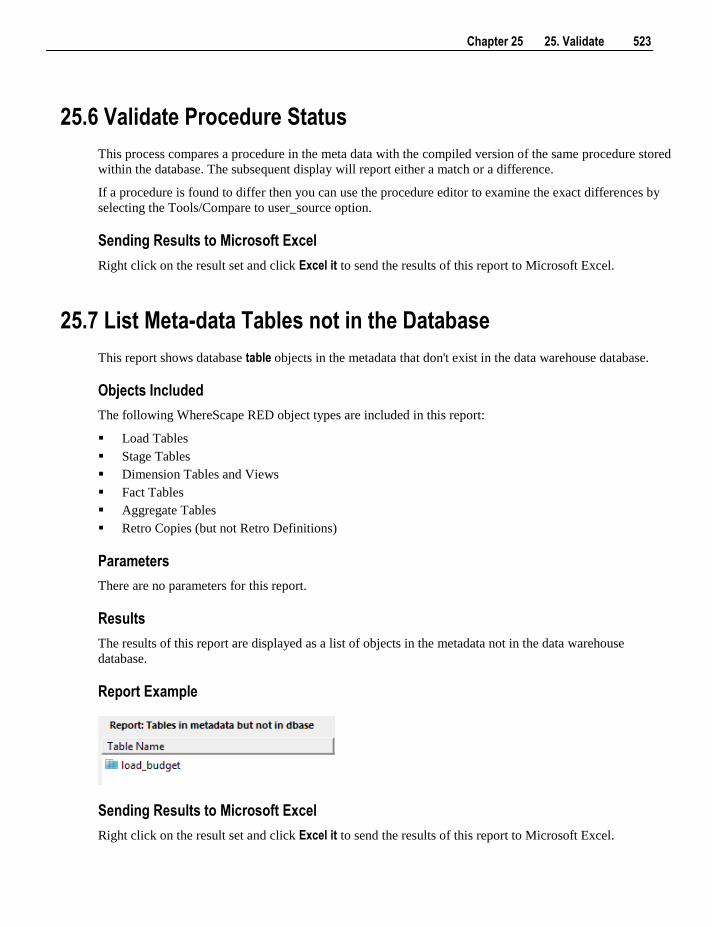
Chapter 25 25. Validate 523
25.6 Validate Procedure Status
This process compares a procedure in the meta data with the compiled version of the same procedure stored
within the database. The subsequent display will report either a match or a difference.
If a procedure is found to differ then you can use the procedure editor to examine the exact differences by
selecting the Tools/Compare to user_source option.
Sending Results to Microsoft Excel
Right click on the result set and click Excel it to send the results of this report to Microsoft Excel.
25.7 List Meta-data Tables not in the Database
This report shows database table objects in the metadata that don't exist in the data warehouse database.
Objects Included
The following WhereScape RED object types are included in this report:
Load Tables
Stage Tables
Dimension Tables and Views
Fact Tables
Aggregate Tables
Retro Copies (but not Retro Definitions)
Parameters
There are no parameters for this report.
Results
The results of this report are displayed as a list of objects in the metadata not in the data warehouse
database.
Report Example
Sending Results to Microsoft Excel
Right click on the result set and click Excel it to send the results of this report to Microsoft Excel.
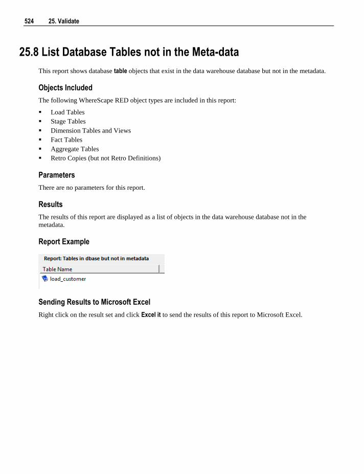
524 25. Validate
25.8 List Database Tables not in the Meta-data
This report shows database table objects that exist in the data warehouse database but not in the metadata.
Objects Included
The following WhereScape RED object types are included in this report:
Load Tables
Stage Tables
Dimension Tables and Views
Fact Tables
Aggregate Tables
Retro Copies (but not Retro Definitions)
Parameters
There are no parameters for this report.
Results
The results of this report are displayed as a list of objects in the data warehouse database not in the
metadata.
Report Example
Sending Results to Microsoft Excel
Right click on the result set and click Excel it to send the results of this report to Microsoft Excel.
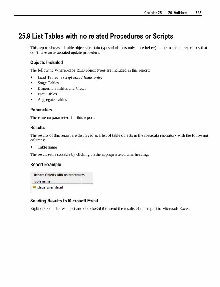
Chapter 25 25. Validate 525
25.9 List Tables with no related Procedures or Scripts
This report shows all table objects (certain types of objects only - see below) in the metadata repository that
don't have an associated update procedure.
Objects Included
The following WhereScape RED object types are included in this report:
Load Tables (script based loads only)
Stage Tables
Dimension Tables and Views
Fact Tables
Aggregate Tables
Parameters
There are no parameters for this report.
Results
The results of this report are displayed as a list of table objects in the metadata repository with the following
columns:
Table name
The result set is sortable by clicking on the appropriate column heading.
Report Example
Sending Results to Microsoft Excel
Right click on the result set and click Excel it to send the results of this report to Microsoft Excel.
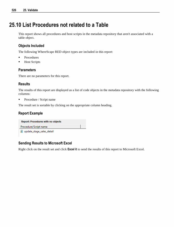
526 25. Validate
25.10 List Procedures not related to a Table
This report shows all procedures and host scripts in the metadata repository that aren't associated with a
table object.
Objects Included
The following WhereScape RED object types are included in this report:
Procedures
Host Scripts
Parameters
There are no parameters for this report.
Results
The results of this report are displayed as a list of code objects in the metadata repository with the following
columns:
Procedure / Script name
The result set is sortable by clicking on the appropriate column heading.
Report Example
Sending Results to Microsoft Excel
Right click on the result set and click Excel it to send the results of this report to Microsoft Excel.
Chapter 25 25. Validate 527
25.11 Compare Meta-data Repository to another
This report compares the current metadata repository to a remote repository.
Objects Included
All object types are included in this report.
Parameters
This report requires connection information for the remote repository to be entered. Specifically:
Odbc Connect (the odbc source for the other repository)
User Name (user name for the remote repository)
Password (password for the remote repository)
Meta Repository (database/user the remote repository metadata is stored in)
Four additional parameters may be specified:
Optional filter on Local Groups
Optional filter on Local Projects
Do detail report
Only validate procedures that have been modified
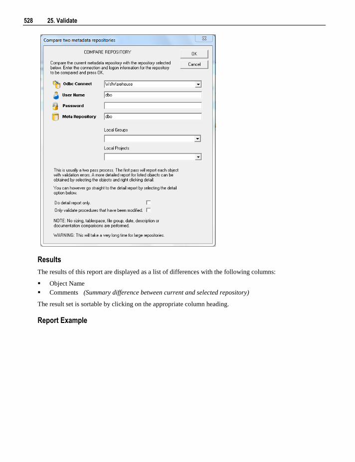
528 25. Validate
Results
The results of this report are displayed as a list of differences with the following columns:
Object Name
Comments (Summary difference between current and selected repository)
The result set is sortable by clicking on the appropriate column heading.
Report Example
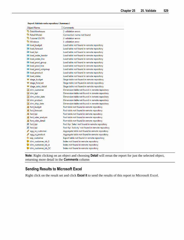
Chapter 25 25. Validate 529
Note: Right clicking on an object and choosing Detail will rerun the report for just the selected object,
returning more detail in the Comments column
Sending Results to Microsoft Excel
Right click on the result set and click Excel it to send the results of this report to Microsoft Excel.
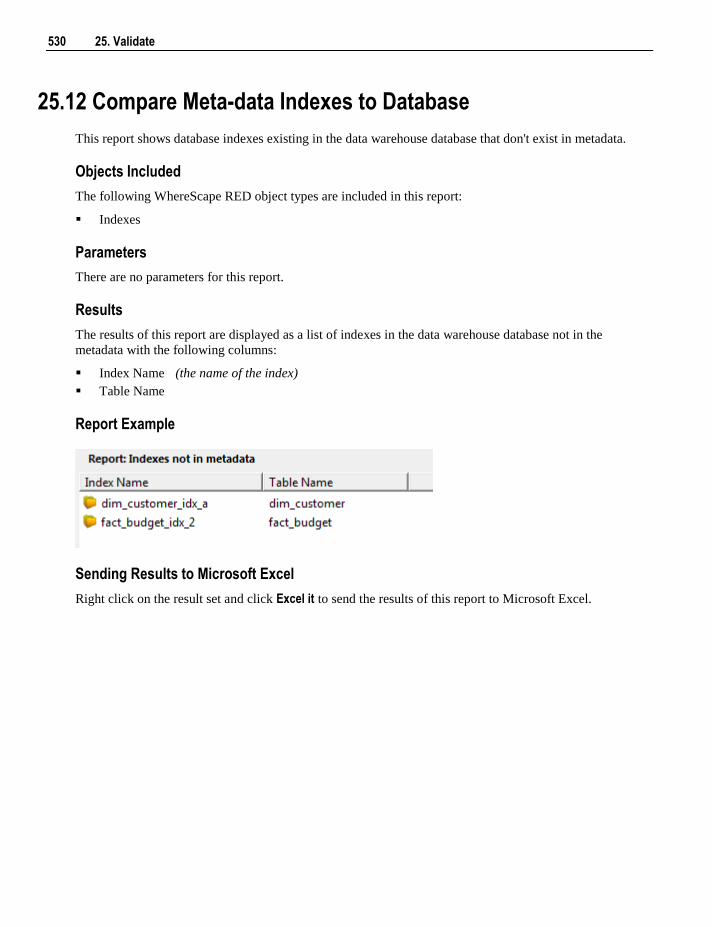
530 25. Validate
25.12 Compare Meta-data Indexes to Database
This report shows database indexes existing in the data warehouse database that don't exist in metadata.
Objects Included
The following WhereScape RED object types are included in this report:
Indexes
Parameters
There are no parameters for this report.
Results
The results of this report are displayed as a list of indexes in the data warehouse database not in the
metadata with the following columns:
Index Name (the name of the index)
Table Name
Report Example
Sending Results to Microsoft Excel
Right click on the result set and click Excel it to send the results of this report to Microsoft Excel.
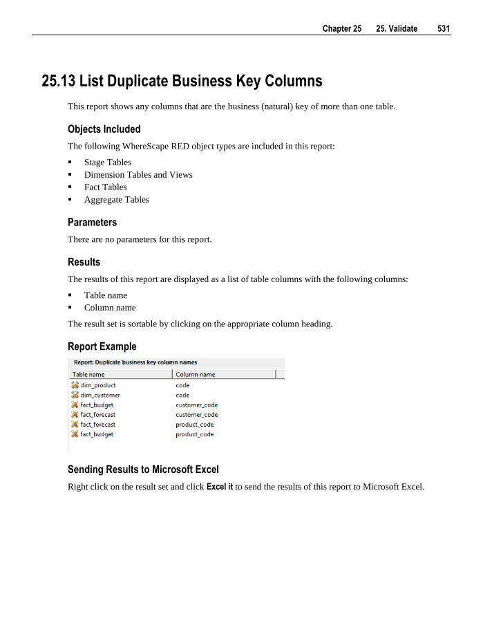
Chapter 25 25. Validate 531
25.13 List Duplicate Business Key Columns
This report shows any columns that are the business (natural) key of more than one table.
Objects Included
The following WhereScape RED object types are included in this report:
Stage Tables
Dimension Tables and Views
Fact Tables
Aggregate Tables
Parameters
There are no parameters for this report.
Results
The results of this report are displayed as a list of table columns with the following columns:
Table name
Column name
The result set is sortable by clicking on the appropriate column heading.
Report Example
Sending Results to Microsoft Excel
Right click on the result set and click Excel it to send the results of this report to Microsoft Excel.
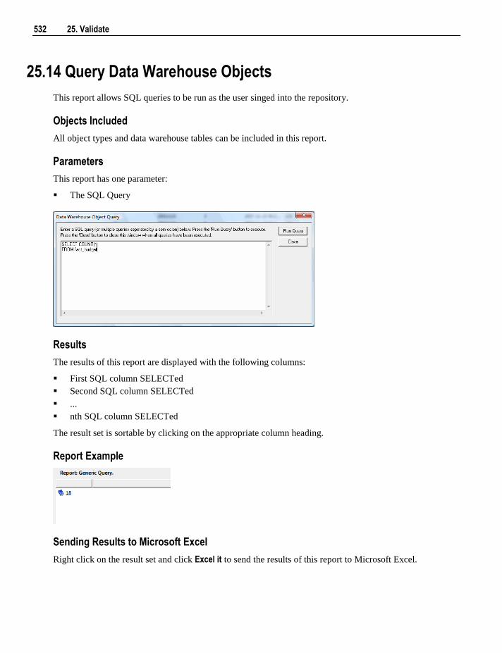
532 25. Validate
25.14 Query Data Warehouse Objects
This report allows SQL queries to be run as the user singed into the repository.
Objects Included
All object types and data warehouse tables can be included in this report.
Parameters
This report has one parameter:
The SQL Query
Results
The results of this report are displayed with the following columns:
First SQL column SELECTed
Second SQL column SELECTed
...
nth SQL column SELECTed
The result set is sortable by clicking on the appropriate column heading.
Report Example
Sending Results to Microsoft Excel
Right click on the result set and click Excel it to send the results of this report to Microsoft Excel.
Chapter 26 26. Promoting Between Environments 533
This chapter covers the promotion of metadata objects between environments. Various methods exist for
getting new or changed metadata from one repository into another repository.
It is of course possible and in fact desirable to have multiple metadata repositories. At the very least we
would normally have a development and a production environment.
In some situations it may also be desirable to have multiple child development repositories with one master
repository where all elements are brought together. WhereScape RED supports this type of structure but
does not include source control or co-ordination of the repositories. It is up to the data warehouse manager
to manually ensure that the various objects are kept in sync and coordinated.
As with any software system there are issues around how code is moved from a development environment
into a testing or production environment.
This promotion of objects can be achieved via a number of different methods. Each is discussed below.
In summary they are:
1 Updating a repository with an application or application patch.
2 Importing objects from another repository.
3 Restoring a full metadata set into a repository (see Backup and Restore (see "27. Backing Up and
Restoring Metadata" on page 547)).
In This Chapter
26.1 Applications ........................................................................ 534
26.2 Importing Object Metadata ................................................. 539
26.3 Importing Language Files ................................................... 540
26.4 Data Warehouse Testing ..................................................... 542
26.5 Creating and Loading Applications from the Command Line 545
C H A P T E R 2 6
26. Promoting Between Environments
534 26. Promoting Between Environments
26.1 Applications
The definition of an application is discussed in the following section on applications and the loading and
updating of applications is discussed at some length in the Installation and Administration Guide. Only the
concepts of the use of applications will be covered here.
An application is defined for our purposes as a group of objects. An application is a method of loading
objects into a metadata repository. It can be used to upgrade or provide patches to an existing metadata
repository. As such an application can be used to distribute and remotely maintain a specific data
warehousing solution.
An application consists of a series of Windows' files, which can be distributed to remote sites.
A list of the applications that have been applied to the metadata repository can be acquired via the Tools / List installed applications menu option.
An application is created through the Tools/Build application tables menu option. This application can then
update a metadata repository through the Setup / Administration utility. In this manner the application
model can be used to update a metadata repository in an ordered and controlled fashion. Loading an
application inserts various objects into the chosen metadata repository. An application is best defined as a
set of objects that are shipped to allow inclusion of those objects in a remote repository.
Note: An application can only be loaded into a metadata repository running on the same database type as
that of the application creator. (e.g. An Oracle application cannot be loaded into a SQL Server metadata
repository, etc).
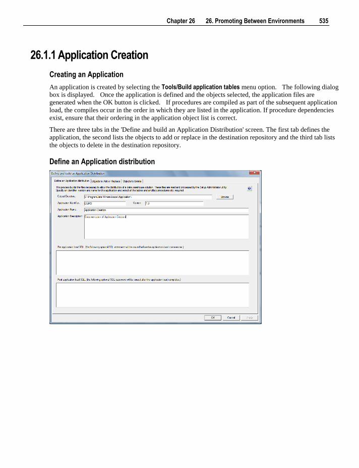
Chapter 26 26. Promoting Between Environments 535
26.1.1 Application Creation
Creating an Application
An application is created by selecting the Tools/Build application tables menu option. The following dialog
box is displayed. Once the application is defined and the objects selected, the application files are
generated when the OK button is clicked. If procedures are compiled as part of the subsequent application
load, the compiles occur in the order in which they are listed in the application. If procedure dependencies
exist, ensure that their ordering in the application object list is correct.
There are three tabs in the 'Define and build an Application Distribution' screen. The first tab defines the
application, the second lists the objects to add or replace in the destination repository and the third tab lists
the objects to delete in the destination repository.
Define an Application distribution
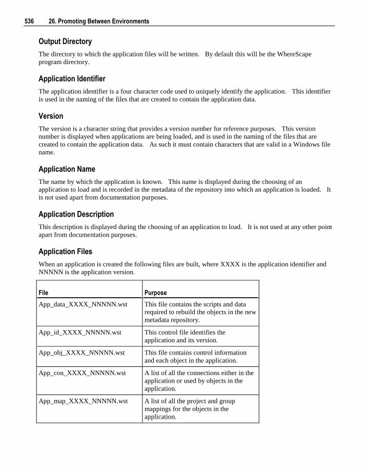
536 26. Promoting Between Environments
Output Directory
The directory to which the application files will be written. By default this will be the WhereScape
program directory.
Application Identifier
The application identifier is a four character code used to uniquely identify the application. This identifier
is used in the naming of the files that are created to contain the application data.
Version
The version is a character string that provides a version number for reference purposes. This version
number is displayed when applications are being loaded, and is used in the naming of the files that are
created to contain the application data. As such it must contain characters that are valid in a Windows file
name.
Application Name
The name by which the application is known. This name is displayed during the choosing of an
application to load and is recorded in the metadata of the repository into which an application is loaded. It
is not used apart from documentation purposes.
Application Description
This description is displayed during the choosing of an application to load. It is not used at any other point
apart from documentation purposes.
Application Files
When an application is created the following files are built, where XXXX is the application identifier and
NNNNN is the application version.
File Purpose
App_data_XXXX_NNNNN.wst This file contains the scripts and data
required to rebuild the objects in the new
metadata repository.
App_id_XXXX_NNNNN.wst This control file identifies the
application and its version.
App_obj_XXXX_NNNNN.wst This file contains control information
and each object in the application.
App_con_XXXX_NNNNN.wst A list of all the connections either in the
application or used by objects in the
application.
App_map_XXXX_NNNNN.wst A list of all the project and group
mappings for the objects in the
application.
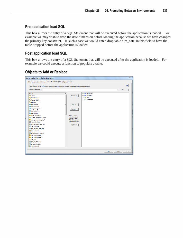
Chapter 26 26. Promoting Between Environments 537
Pre application load SQL
This box allows the entry of a SQL Statement that will be executed before the application is loaded. For
example we may wish to drop the date dimension before loading the application because we have changed
the primary key constraint. In such a case we would enter 'drop table dim_date' in this field to have the
table dropped before the application is loaded.
Post application load SQL
This box allows the entry of a SQL Statement that will be executed after the application is loaded. For
example we could execute a function to populate a table.
Objects to Add or Replace
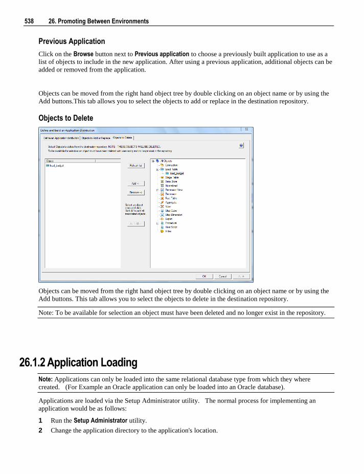
538 26. Promoting Between Environments
Previous Application
Click on the Browse button next to Previous application to choose a previously built application to use as a
list of objects to include in the new application. After using a previous application, additional objects can be
added or removed from the application.
Objects can be moved from the right hand object tree by double clicking on an object name or by using the
Add buttons.This tab allows you to select the objects to add or replace in the destination repository.
Objects to Delete
Objects can be moved from the right hand object tree by double clicking on an object name or by using the
Add buttons. This tab allows you to select the objects to delete in the destination repository.
Note: To be available for selection an object must have been deleted and no longer exist in the repository.
26.1.2 Application Loading
Note: Applications can only be loaded into the same relational database type from which they where
created. (For Example an Oracle application can only be loaded into an Oracle database).
Applications are loaded via the Setup Administrator utility. The normal process for implementing an
application would be as follows:
1 Run the Setup Administrator utility.
2 Change the application directory to the application's location.
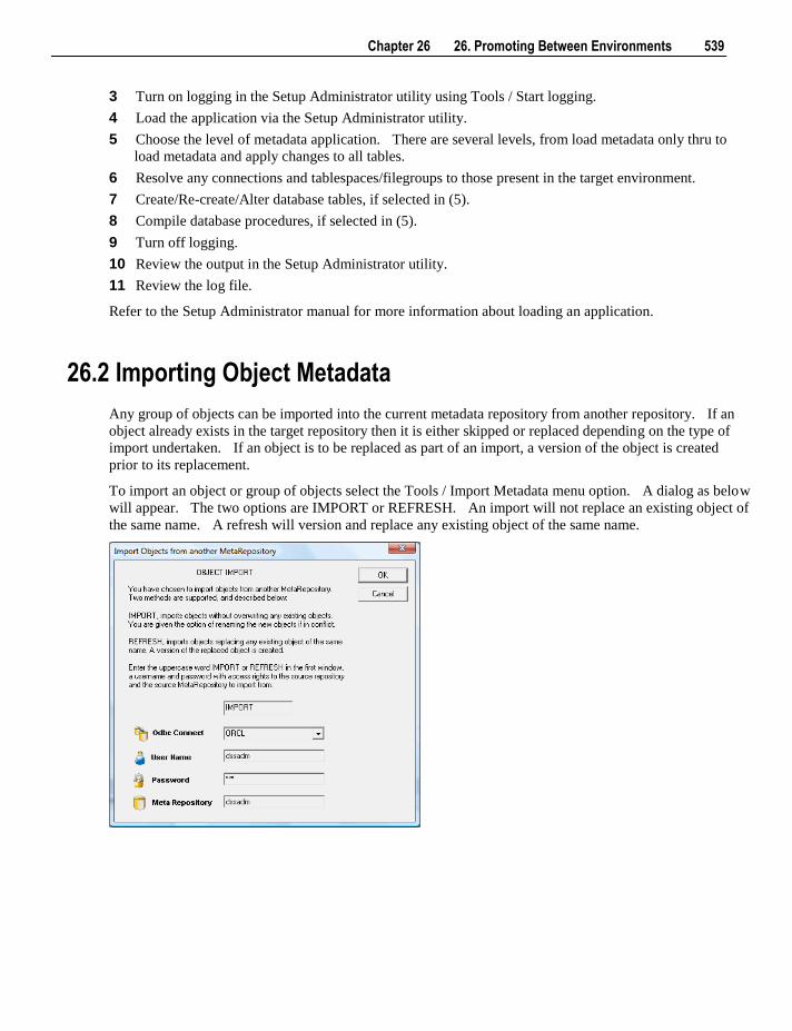
Chapter 26 26. Promoting Between Environments 539
3 Turn on logging in the Setup Administrator utility using Tools / Start logging.
4 Load the application via the Setup Administrator utility.
5 Choose the level of metadata application. There are several levels, from load metadata only thru to
load metadata and apply changes to all tables.
6 Resolve any connections and tablespaces/filegroups to those present in the target environment.
7 Create/Re-create/Alter database tables, if selected in (5).
8 Compile database procedures, if selected in (5).
9 Turn off logging.
10 Review the output in the Setup Administrator utility.
11 Review the log file.
Refer to the Setup Administrator manual for more information about loading an application.
26.2 Importing Object Metadata
Any group of objects can be imported into the current metadata repository from another repository. If an
object already exists in the target repository then it is either skipped or replaced depending on the type of
import undertaken. If an object is to be replaced as part of an import, a version of the object is created
prior to its replacement.
To import an object or group of objects select the Tools / Import Metadata menu option. A dialog as below
will appear. The two options are IMPORT or REFRESH. An import will not replace an existing object of
the same name. A refresh will version and replace any existing object of the same name.
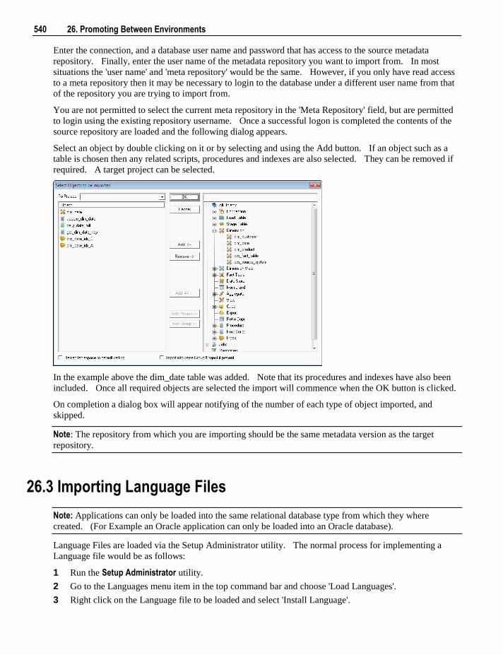
540 26. Promoting Between Environments
Enter the connection, and a database user name and password that has access to the source metadata
repository. Finally, enter the user name of the metadata repository you want to import from. In most
situations the 'user name' and 'meta repository' would be the same. However, if you only have read access
to a meta repository then it may be necessary to login to the database under a different user name from that
of the repository you are trying to import from.
You are not permitted to select the current meta repository in the 'Meta Repository' field, but are permitted
to login using the existing repository username. Once a successful logon is completed the contents of the
source repository are loaded and the following dialog appears.
Select an object by double clicking on it or by selecting and using the Add button. If an object such as a
table is chosen then any related scripts, procedures and indexes are also selected. They can be removed if
required. A target project can be selected.
In the example above the dim_date table was added. Note that its procedures and indexes have also been
included. Once all required objects are selected the import will commence when the OK button is clicked.
On completion a dialog box will appear notifying of the number of each type of object imported, and
skipped.
Note: The repository from which you are importing should be the same metadata version as the target
repository.
26.3 Importing Language Files
Note: Applications can only be loaded into the same relational database type from which they where
created. (For Example an Oracle application can only be loaded into an Oracle database).
Language Files are loaded via the Setup Administrator utility. The normal process for implementing a
Language file would be as follows:
1 Run the Setup Administrator utility.
2 Go to the Languages menu item in the top command bar and choose 'Load Languages'.
3 Right click on the Language file to be loaded and select 'Install Language'.
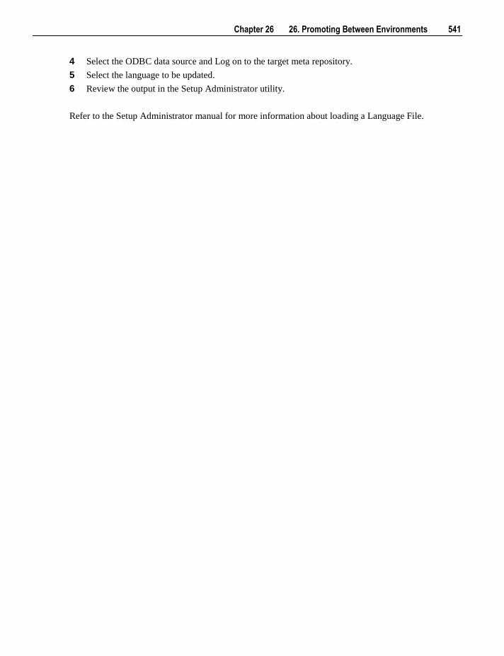
Chapter 26 26. Promoting Between Environments 541
4 Select the ODBC data source and Log on to the target meta repository.
5 Select the language to be updated.
6 Review the output in the Setup Administrator utility.
Refer to the Setup Administrator manual for more information about loading a Language File.
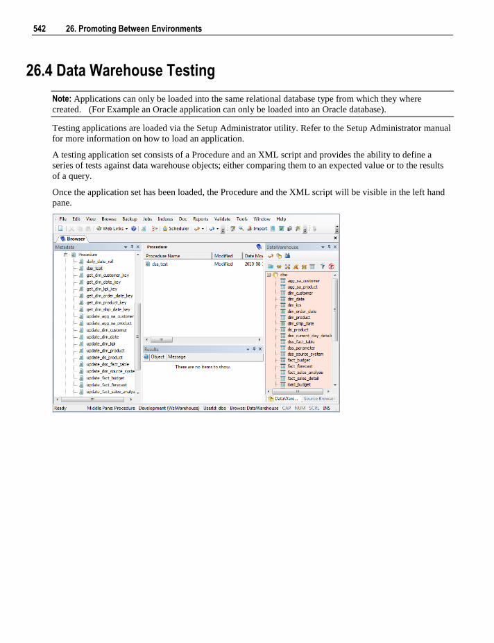
542 26. Promoting Between Environments
26.4 Data Warehouse Testing
Note: Applications can only be loaded into the same relational database type from which they where
created. (For Example an Oracle application can only be loaded into an Oracle database).
Testing applications are loaded via the Setup Administrator utility. Refer to the Setup Administrator manual
for more information on how to load an application.
A testing application set consists of a Procedure and an XML script and provides the ability to define a
series of tests against data warehouse objects; either comparing them to an expected value or to the results
of a query.
Once the application set has been loaded, the Procedure and the XML script will be visible in the left hand
pane.
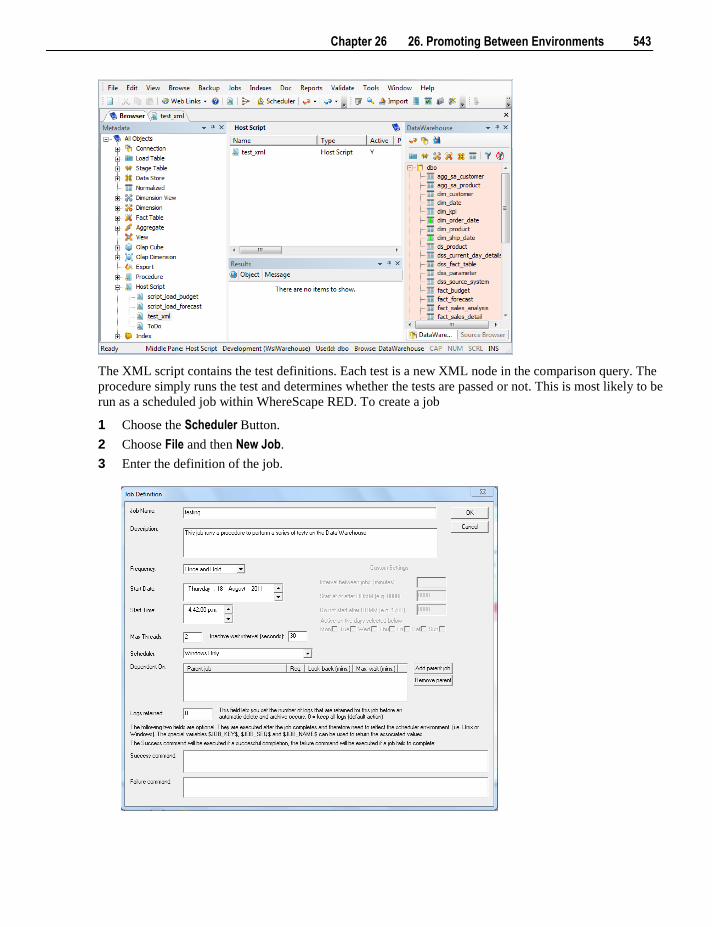
Chapter 26 26. Promoting Between Environments 543
The XML script contains the test definitions. Each test is a new XML node in the comparison query. The
procedure simply runs the test and determines whether the tests are passed or not. This is most likely to be
run as a scheduled job within WhereScape RED. To create a job
1 Choose the Scheduler Button.
2 Choose File and then New Job.
3 Enter the definition of the job.
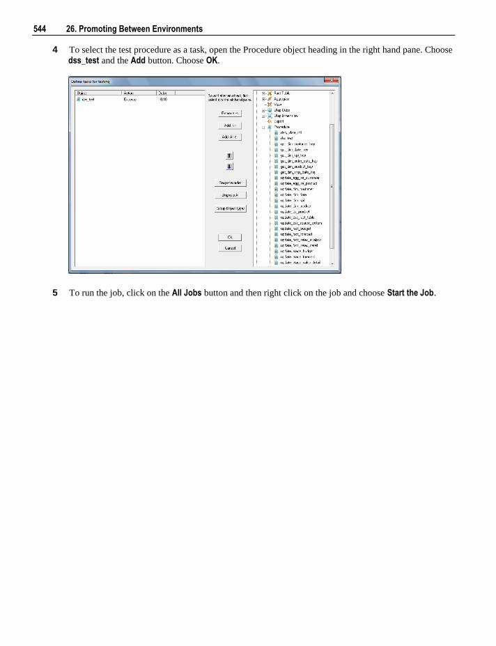
544 26. Promoting Between Environments
4 To select the test procedure as a task, open the Procedure object heading in the right hand pane. Choose
dss_test and the Add button. Choose OK.
5 To run the job, click on the All Jobs button and then right click on the job and choose Start the Job.
Chapter 26 26. Promoting Between Environments 545
26.5 Creating and Loading Applications from the Command Line
It is possible to create and load applications from the command line by running a bat file. The WhereScape
RED Application directory contains an example bat file
WSL_Application_Create_Restore_Point_and_Load.bat for creating and loading.
If you right mouse on this file and choose Edit you will see the steps outlined as well as the details on the
options available.
The first step creates a restore point application (R) based on objects about to be loaded. This process calls
the command line functionality of RED and creates the application file.
The second step loads an application (A) into a test WhereScape RED repository. It uses an xml file to
specify various options, calls the command line automation functionality of Setup Administrator and loads
the application (A). The WhereScape RED Application directory contains example xml files:
WSL_Application_Load_SQL.xml for SQL Server
WSL_Application_Load_DB2.xml for DB2
WSL_Application_Load_ORA.xml for Oracle
The tags in the xml file need to be edited as the login/connection details etc need setting.
The Batch Application Create options and the Batch Application Load options are listed at the end of the
bat file. The values for these variables will also need to be customized before running this file.
The process typically involves the following steps:
1 Create an application (A) in RED containing your data warehouse changes.
2 RUN WSL_Application_Create_Restore_Point_and_Load.bat from the command line; which creates a
restore point application (R) and applies application (A) to a test WhereScape RED repository.
3 If the changes are incorrect, they can be undone by loading the restore point application (R).
Note: You can only create a RESTORE application through the command line; deployment applications are
still built through RED.

Chapter 27 27. Backing Up and Restoring Metadata 547
This chapter covers the saving and reloading of metadata repository objects. The backup section describes
the methods for backing up the metadata repository. It can also be backed up via normal database backup
procedures. The restore section covers the metadata restoration functions available.
WhereScape RED provides two different methods for backing up and restoring metadata:
1 Backup and Restore using the native backup tools available in the data warehouse database.
2 WhereScape RED unload and load.
In This Chapter
27.1 Backup using DB Routines ................................................. 548
27.2 Restoring DB Backups ........................................................ 551
27.3 Unloading Metadata ............................................................ 555
27.4 Loading an Unload .............................................................. 556
C H A P T E R 2 7
27. Backing Up and Restoring Metadata
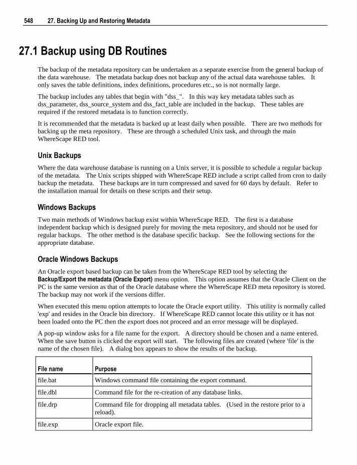
548 27. Backing Up and Restoring Metadata
27.1 Backup using DB Routines
The backup of the metadata repository can be undertaken as a separate exercise from the general backup of
the data warehouse. The metadata backup does not backup any of the actual data warehouse tables. It
only saves the table definitions, index definitions, procedures etc., so is not normally large.
The backup includes any tables that begin with "dss_". In this way key metadata tables such as
dss_parameter, dss_source_system and dss_fact_table are included in the backup. These tables are
required if the restored metadata is to function correctly.
It is recommended that the metadata is backed up at least daily when possible. There are two methods for
backing up the meta repository. These are through a scheduled Unix task, and through the main
WhereScape RED tool.
Unix Backups
Where the data warehouse database is running on a Unix server, it is possible to schedule a regular backup
of the metadata. The Unix scripts shipped with WhereScape RED include a script called from cron to daily
backup the metadata. These backups are in turn compressed and saved for 60 days by default. Refer to
the installation manual for details on these scripts and their setup.
Windows Backups
Two main methods of Windows backup exist within WhereScape RED. The first is a database
independent backup which is designed purely for moving the meta repository, and should not be used for
regular backups. The other method is the database specific backup. See the following sections for the
appropriate database.
Oracle Windows Backups
An Oracle export based backup can be taken from the WhereScape RED tool by selecting the
Backup/Export the metadata (Oracle Export) menu option. This option assumes that the Oracle Client on the
PC is the same version as that of the Oracle database where the WhereScape RED meta repository is stored.
The backup may not work if the versions differ.
When executed this menu option attempts to locate the Oracle export utility. This utility is normally called
'exp' and resides in the Oracle bin directory. If WhereScape RED cannot locate this utility or it has not
been loaded onto the PC then the export does not proceed and an error message will be displayed.
A pop-up window asks for a file name for the export. A directory should be chosen and a name entered.
When the save button is clicked the export will start. The following files are created (where 'file' is the
name of the chosen file). A dialog box appears to show the results of the backup.
File name Purpose
file.bat Windows command file containing the export command.
file.dbl Command file for the re-creation of any database links.
file.drp Command file for dropping all metadata tables. (Used in the restore prior to a
reload).
file.exp Oracle export file.
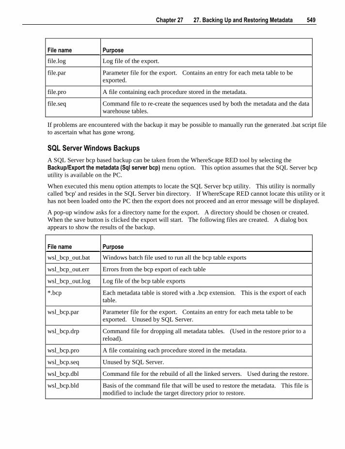
Chapter 27 27. Backing Up and Restoring Metadata 549
File name Purpose
file.log Log file of the export.
file.par Parameter file for the export. Contains an entry for each meta table to be
exported.
file.pro A file containing each procedure stored in the metadata.
file.seq Command file to re-create the sequences used by both the metadata and the data
warehouse tables.
If problems are encountered with the backup it may be possible to manually run the generated .bat script file
to ascertain what has gone wrong.
SQL Server Windows Backups
A SQL Server bcp based backup can be taken from the WhereScape RED tool by selecting the
Backup/Export the metadata (Sql server bcp) menu option. This option assumes that the SQL Server bcp
utility is available on the PC.
When executed this menu option attempts to locate the SQL Server bcp utility. This utility is normally
called 'bcp' and resides in the SQL Server bin directory. If WhereScape RED cannot locate this utility or it
has not been loaded onto the PC then the export does not proceed and an error message will be displayed.
A pop-up window asks for a directory name for the export. A directory should be chosen or created.
When the save button is clicked the export will start. The following files are created. A dialog box
appears to show the results of the backup.
File name Purpose
wsl_bcp_out.bat Windows batch file used to run all the bcp table exports
wsl_bcp_out.err Errors from the bcp export of each table
wsl_bcp_out.log Log file of the bcp table exports
*.bcp Each metadata table is stored with a .bcp extension. This is the export of each
table.
wsl_bcp.par Parameter file for the export. Contains an entry for each meta table to be
exported. Unused by SQL Server.
wsl_bcp.drp Command file for dropping all metadata tables. (Used in the restore prior to a
reload).
wsl_bcp.pro A file containing each procedure stored in the metadata.
wsl_bcp.seq Unused by SQL Server.
wsl_bcp.dbl Command file for the rebuild of all the linked servers. Used during the restore.
wsl_bcp.bld Basis of the command file that will be used to restore the metadata. This file is
modified to include the target directory prior to restore.
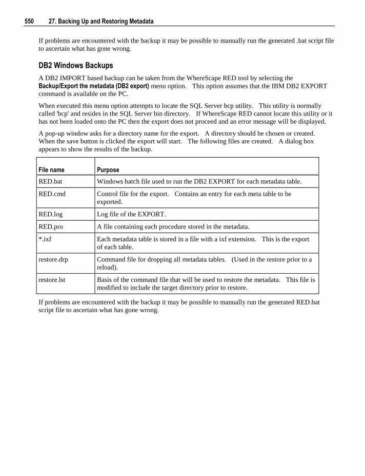
550 27. Backing Up and Restoring Metadata
If problems are encountered with the backup it may be possible to manually run the generated .bat script file
to ascertain what has gone wrong.
DB2 Windows Backups
A DB2 IMPORT based backup can be taken from the WhereScape RED tool by selecting the
Backup/Export the metadata (DB2 export) menu option. This option assumes that the IBM DB2 EXPORT
command is available on the PC.
When executed this menu option attempts to locate the SQL Server bcp utility. This utility is normally
called 'bcp' and resides in the SQL Server bin directory. If WhereScape RED cannot locate this utility or it
has not been loaded onto the PC then the export does not proceed and an error message will be displayed.
A pop-up window asks for a directory name for the export. A directory should be chosen or created.
When the save button is clicked the export will start. The following files are created. A dialog box
appears to show the results of the backup.
File name Purpose
RED.bat Windows batch file used to run the DB2 EXPORT for each metadata table.
RED.cmd Control file for the export. Contains an entry for each meta table to be
exported.
RED.log Log file of the EXPORT.
RED.pro A file containing each procedure stored in the metadata.
*.ixf Each metadata table is stored in a file with a ixf extension. This is the export
of each table.
restore.drp Command file for dropping all metadata tables. (Used in the restore prior to a
reload).
restore.lst Basis of the command file that will be used to restore the metadata. This file is
modified to include the target directory prior to restore.
If problems are encountered with the backup it may be possible to manually run the generated RED.bat
script file to ascertain what has gone wrong.
Chapter 27 27. Backing Up and Restoring Metadata 551
27.2 Restoring DB Backups
WhereScape RED metadata can be restored from a prior backup. For Oracle data warehouses the restore
can take place either from Unix or through the WhereScape RED tool. The same set of files as defined in
the backup section are used for both restores and can be moved between the Windows and Unix
environments. For SQL Server data warehouses the restore must take place in a Windows environment
either through the WhereScape RED tool or manually.
Note: If transferring the export files via ftp, ensure that the file.exp and .bcp files are transferred in binary
mode and that the other files are transferred in ASCII mode.
Restoring metadata
A backup of a metadata repository can be restored over the top of an existing repository. This action
replaces the existing repository in its entirety. The restore of repositories is covered in an earlier section,
but its uses in the promoting of code are discussed here. This restore process does not affect any existing
database tables or any compiled procedures, so it can be used as a means of updating a metadata repository,
albeit by replacing that repository. It is often a good method to choose when first establishing a new
repository. For example if we have a development repository and want to create a production environment
the steps may be:
1 Backup the development repository, using either the Unix or Windows repository backup. See the
previous sections.
2 Create a new repository using the Setup / Administrator utility.
3 Log on to the newly created repository.
4 Restore the backup of the development repository into the new repository. For Oracle this requires the
database privilege 'imp_full_database', or the dba role.
5 Modify any connections, set any default values, alter any table sizes or extents.
6 Create the tables.
7 Compile all procedures.
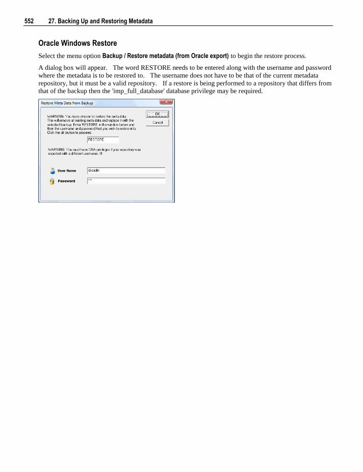
552 27. Backing Up and Restoring Metadata
Oracle Windows Restore
Select the menu option Backup / Restore metadata (from Oracle export) to begin the restore process.
A dialog box will appear. The word RESTORE needs to be entered along with the username and password
where the metadata is to be restored to. The username does not have to be that of the current metadata
repository, but it must be a valid repository. If a restore is being performed to a repository that differs from
that of the backup then the 'imp_full_database' database privilege may be required.
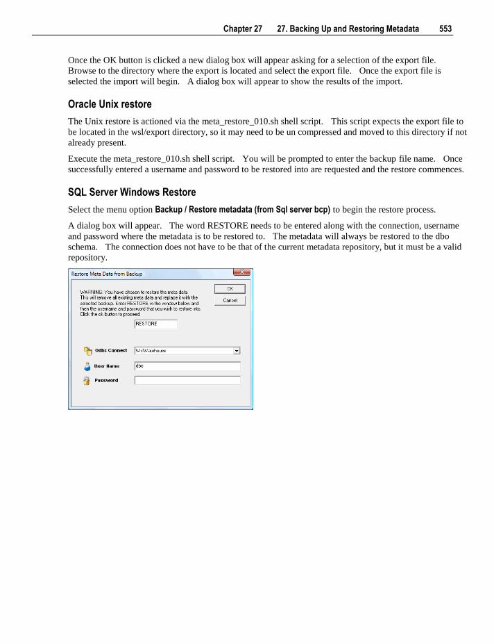
Chapter 27 27. Backing Up and Restoring Metadata 553
Once the OK button is clicked a new dialog box will appear asking for a selection of the export file.
Browse to the directory where the export is located and select the export file. Once the export file is
selected the import will begin. A dialog box will appear to show the results of the import.
Oracle Unix restore
The Unix restore is actioned via the meta_restore_010.sh shell script. This script expects the export file to
be located in the wsl/export directory, so it may need to be un compressed and moved to this directory if not
already present.
Execute the meta_restore_010.sh shell script. You will be prompted to enter the backup file name. Once
successfully entered a username and password to be restored into are requested and the restore commences.
SQL Server Windows Restore
Select the menu option Backup / Restore metadata (from Sql server bcp) to begin the restore process.
A dialog box will appear. The word RESTORE needs to be entered along with the connection, username
and password where the metadata is to be restored to. The metadata will always be restored to the dbo
schema. The connection does not have to be that of the current metadata repository, but it must be a valid
repository.
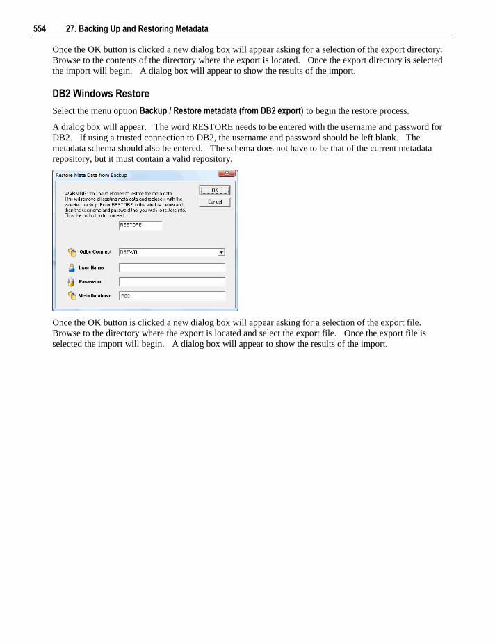
554 27. Backing Up and Restoring Metadata
Once the OK button is clicked a new dialog box will appear asking for a selection of the export directory.
Browse to the contents of the directory where the export is located. Once the export directory is selected
the import will begin. A dialog box will appear to show the results of the import.
DB2 Windows Restore
Select the menu option Backup / Restore metadata (from DB2 export) to begin the restore process.
A dialog box will appear. The word RESTORE needs to be entered with the username and password for
DB2. If using a trusted connection to DB2, the username and password should be left blank. The
metadata schema should also be entered. The schema does not have to be that of the current metadata
repository, but it must contain a valid repository.
Once the OK button is clicked a new dialog box will appear asking for a selection of the export file.
Browse to the directory where the export is located and select the export file. Once the export file is
selected the import will begin. A dialog box will appear to show the results of the import.
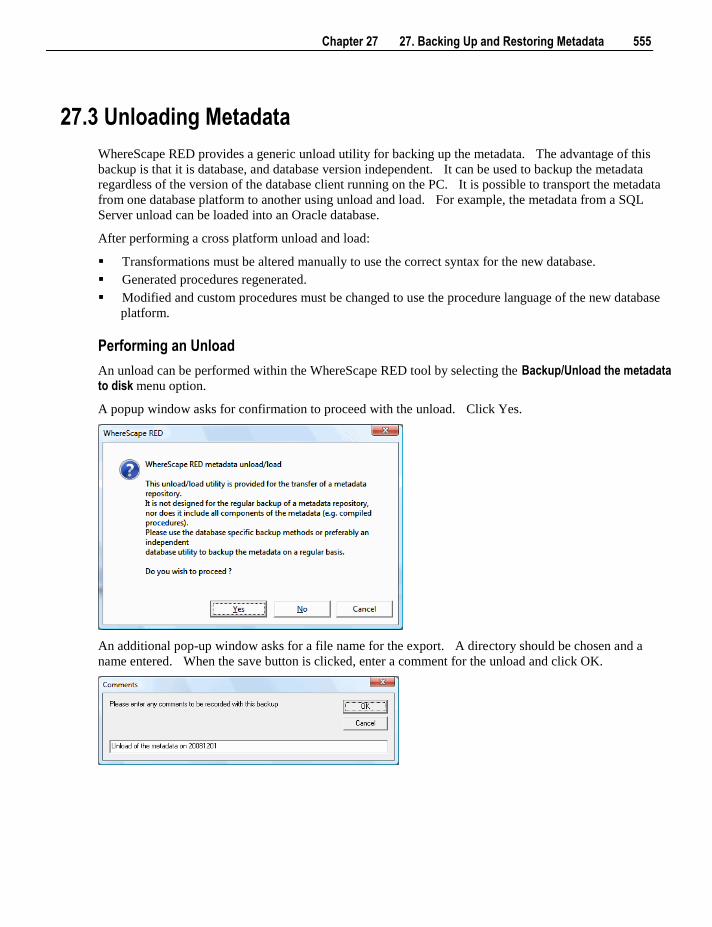
Chapter 27 27. Backing Up and Restoring Metadata 555
27.3 Unloading Metadata
WhereScape RED provides a generic unload utility for backing up the metadata. The advantage of this
backup is that it is database, and database version independent. It can be used to backup the metadata
regardless of the version of the database client running on the PC. It is possible to transport the metadata
from one database platform to another using unload and load. For example, the metadata from a SQL
Server unload can be loaded into an Oracle database.
After performing a cross platform unload and load:
Transformations must be altered manually to use the correct syntax for the new database.
Generated procedures regenerated.
Modified and custom procedures must be changed to use the procedure language of the new database
platform.
Performing an Unload
An unload can be performed within the WhereScape RED tool by selecting the Backup/Unload the metadata to disk menu option.
A popup window asks for confirmation to proceed with the unload. Click Yes.
An additional pop-up window asks for a file name for the export. A directory should be chosen and a
name entered. When the save button is clicked, enter a comment for the unload and click OK.
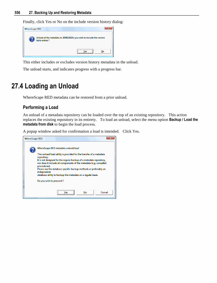
556 27. Backing Up and Restoring Metadata
Finally, click Yes or No on the include version history dialog:
This either includes or excludes version history metadata in the unload.
The unload starts, and indicates progress with a progress bar.
27.4 Loading an Unload
WhereScape RED metadata can be restored from a prior unload.
Performing a Load
An unload of a metadata repository can be loaded over the top of an existing repository. This action
replaces the existing repository in its entirety. To load an unload, select the menu option Backup / Load the metadata from disk to begin the load process.
A popup window asked for confirmation a load is intended. Click Yes.
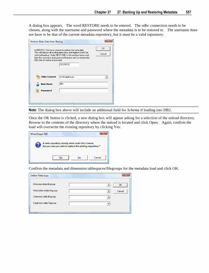
Chapter 27 27. Backing Up and Restoring Metadata 557
A dialog box appears. The word RESTORE needs to be entered. The odbc connection needs to be
chosen, along with the username and password where the metadata is to be restored to. The username does
not have to be that of the current metadata repository, but it must be a valid repository.
Note: The dialog box above will include an additional field for Schema if loading into DB2.
Once the OK button is clicked, a new dialog box will appear asking for a selection of the unload directory.
Browse to the contents of the directory where the unload is located and click Open. Again, confirm the
load will overwrite the existing repository by clicking Yes:
Confirm the metadata and dimension tablespaces/filegroups for the metadata load and click OK:
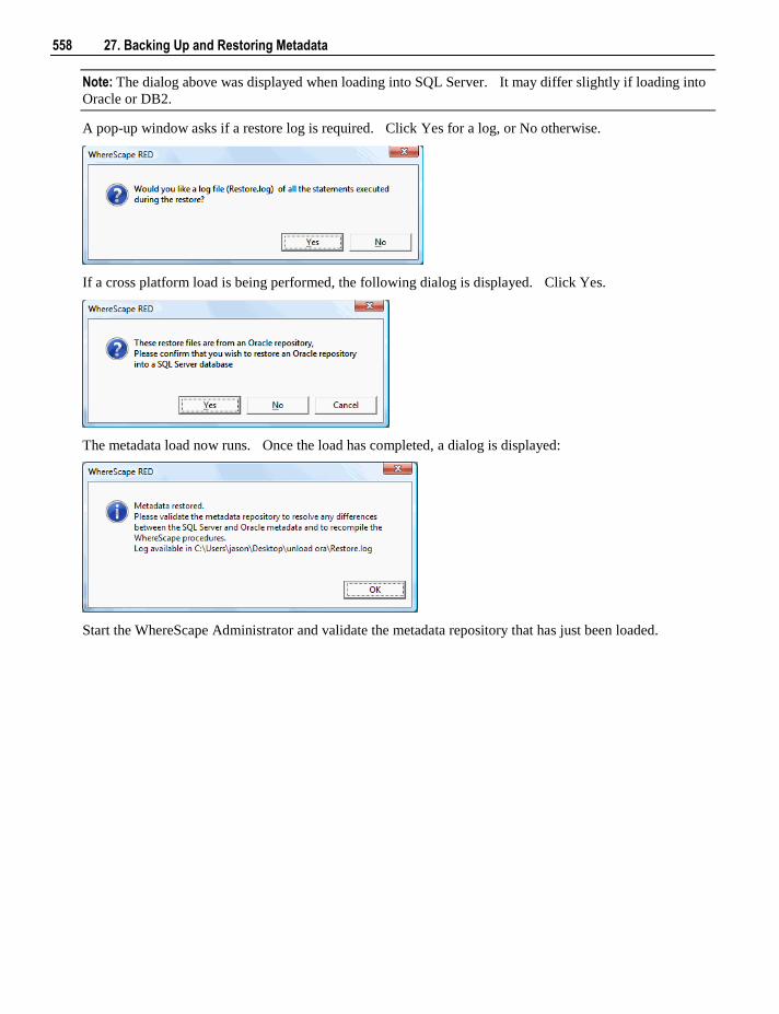
558 27. Backing Up and Restoring Metadata
Note: The dialog above was displayed when loading into SQL Server. It may differ slightly if loading into
Oracle or DB2.
A pop-up window asks if a restore log is required. Click Yes for a log, or No otherwise.
If a cross platform load is being performed, the following dialog is displayed. Click Yes.
The metadata load now runs. Once the load has completed, a dialog is displayed:
Start the WhereScape Administrator and validate the metadata repository that has just been loaded.
Chapter 28 28. Altering Metadata 559
This chapter provides information on how to change and manipulate the data warehouse once it has been
established.
New source columns or changes to the source systems from which the data warehouse is built will require
modifications to both the metadata and the data warehouse tables and procedures.
In This Chapter
28.1 Validating Tables ................................................................ 560
28.2 Validating Source (Load) Tables ........................................ 562
28.3 Validating Procedures ......................................................... 562
28.4 Altering Tables .................................................................... 563
28.5 Validating Indexes .............................................................. 564
28.6 Recompiling Procedures ..................................................... 564
C H A P T E R 2 8
28. Altering Metadata
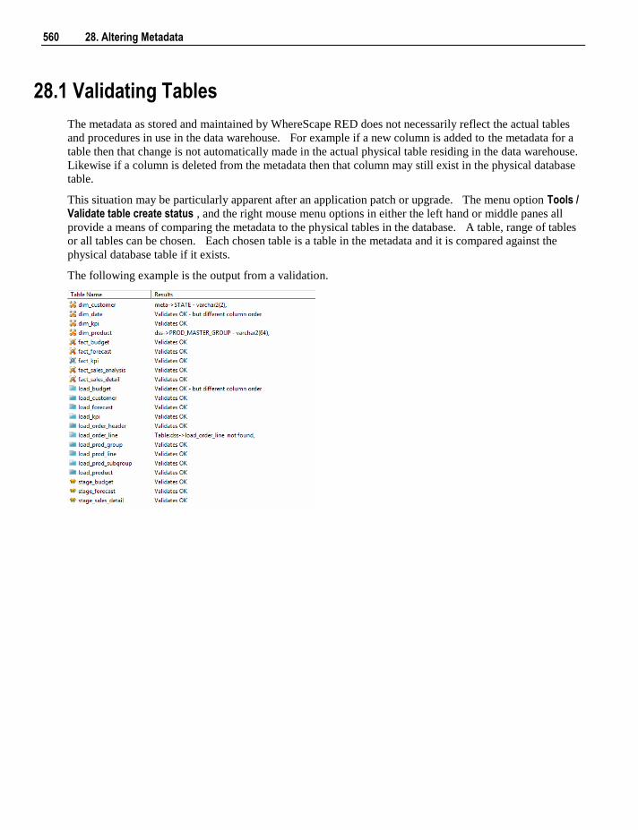
560 28. Altering Metadata
28.1 Validating Tables
The metadata as stored and maintained by WhereScape RED does not necessarily reflect the actual tables
and procedures in use in the data warehouse. For example if a new column is added to the metadata for a
table then that change is not automatically made in the actual physical table residing in the data warehouse.
Likewise if a column is deleted from the metadata then that column may still exist in the physical database
table.
This situation may be particularly apparent after an application patch or upgrade. The menu option Tools / Validate table create status , and the right mouse menu options in either the left hand or middle panes all
provide a means of comparing the metadata to the physical tables in the database. A table, range of tables
or all tables can be chosen. Each chosen table is a table in the metadata and it is compared against the
physical database table if it exists.
The following example is the output from a validation.
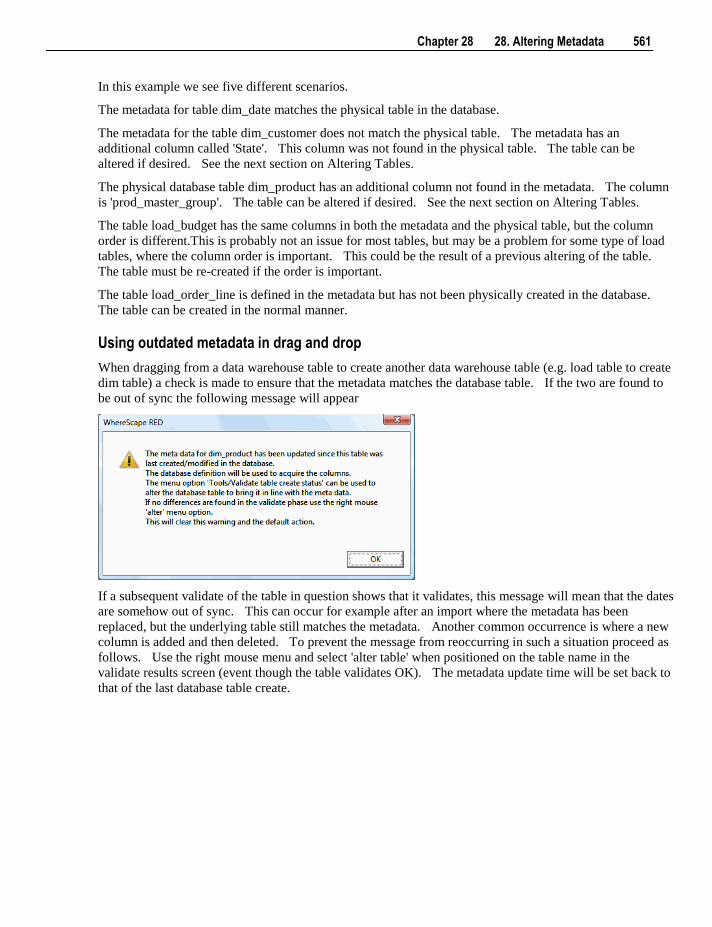
Chapter 28 28. Altering Metadata 561
In this example we see five different scenarios.
The metadata for table dim_date matches the physical table in the database.
The metadata for the table dim_customer does not match the physical table. The metadata has an
additional column called 'State'. This column was not found in the physical table. The table can be
altered if desired. See the next section on Altering Tables.
The physical database table dim_product has an additional column not found in the metadata. The column
is 'prod_master_group'. The table can be altered if desired. See the next section on Altering Tables.
The table load_budget has the same columns in both the metadata and the physical table, but the column
order is different.This is probably not an issue for most tables, but may be a problem for some type of load
tables, where the column order is important. This could be the result of a previous altering of the table.
The table must be re-created if the order is important.
The table load_order_line is defined in the metadata but has not been physically created in the database.
The table can be created in the normal manner.
Using outdated metadata in drag and drop
When dragging from a data warehouse table to create another data warehouse table (e.g. load table to create
dim table) a check is made to ensure that the metadata matches the database table. If the two are found to
be out of sync the following message will appear
If a subsequent validate of the table in question shows that it validates, this message will mean that the dates
are somehow out of sync. This can occur for example after an import where the metadata has been
replaced, but the underlying table still matches the metadata. Another common occurrence is where a new
column is added and then deleted. To prevent the message from reoccurring in such a situation proceed as
follows. Use the right mouse menu and select 'alter table' when positioned on the table name in the
validate results screen (event though the table validates OK). The metadata update time will be set back to
that of the last database table create.
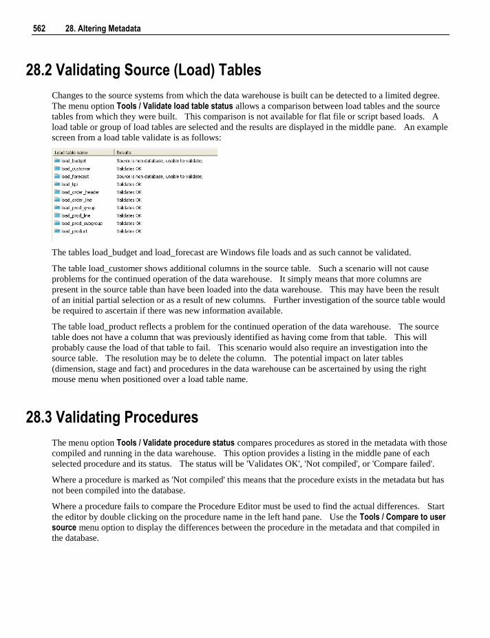
562 28. Altering Metadata
28.2 Validating Source (Load) Tables
Changes to the source systems from which the data warehouse is built can be detected to a limited degree.
The menu option Tools / Validate load table status allows a comparison between load tables and the source
tables from which they were built. This comparison is not available for flat file or script based loads. A
load table or group of load tables are selected and the results are displayed in the middle pane. An example
screen from a load table validate is as follows:
The tables load_budget and load_forecast are Windows file loads and as such cannot be validated.
The table load_customer shows additional columns in the source table. Such a scenario will not cause
problems for the continued operation of the data warehouse. It simply means that more columns are
present in the source table than have been loaded into the data warehouse. This may have been the result
of an initial partial selection or as a result of new columns. Further investigation of the source table would
be required to ascertain if there was new information available.
The table load_product reflects a problem for the continued operation of the data warehouse. The source
table does not have a column that was previously identified as having come from that table. This will
probably cause the load of that table to fail. This scenario would also require an investigation into the
source table. The resolution may be to delete the column. The potential impact on later tables
(dimension, stage and fact) and procedures in the data warehouse can be ascertained by using the right
mouse menu when positioned over a load table name.
28.3 Validating Procedures
The menu option Tools / Validate procedure status compares procedures as stored in the metadata with those
compiled and running in the data warehouse. This option provides a listing in the middle pane of each
selected procedure and its status. The status will be 'Validates OK', 'Not compiled', or 'Compare failed'.
Where a procedure is marked as 'Not compiled' this means that the procedure exists in the metadata but has
not been compiled into the database.
Where a procedure fails to compare the Procedure Editor must be used to find the actual differences. Start
the editor by double clicking on the procedure name in the left hand pane. Use the Tools / Compare to user source menu option to display the differences between the procedure in the metadata and that compiled in
the database.
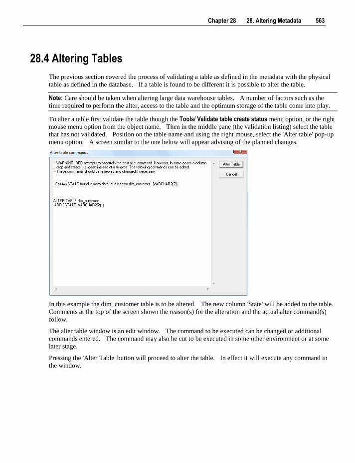
Chapter 28 28. Altering Metadata 563
28.4 Altering Tables
The previous section covered the process of validating a table as defined in the metadata with the physical
table as defined in the database. If a table is found to be different it is possible to alter the table.
Note: Care should be taken when altering large data warehouse tables. A number of factors such as the
time required to perform the alter, access to the table and the optimum storage of the table come into play.
To alter a table first validate the table though the Tools/ Validate table create status menu option, or the right
mouse menu option from the object name. Then in the middle pane (the validation listing) select the table
that has not validated. Position on the table name and using the right mouse, select the 'Alter table' pop-up
menu option. A screen similar to the one below will appear advising of the planned changes.
In this example the dim_customer table is to be altered. The new column 'State' will be added to the table.
Comments at the top of the screen shown the reason(s) for the alteration and the actual alter command(s)
follow.
The alter table window is an edit window. The command to be executed can be changed or additional
commands entered. The command may also be cut to be executed in some other environment or at some
later stage.
Pressing the 'Alter Table' button will proceed to alter the table. In effect it will execute any command in
the window.
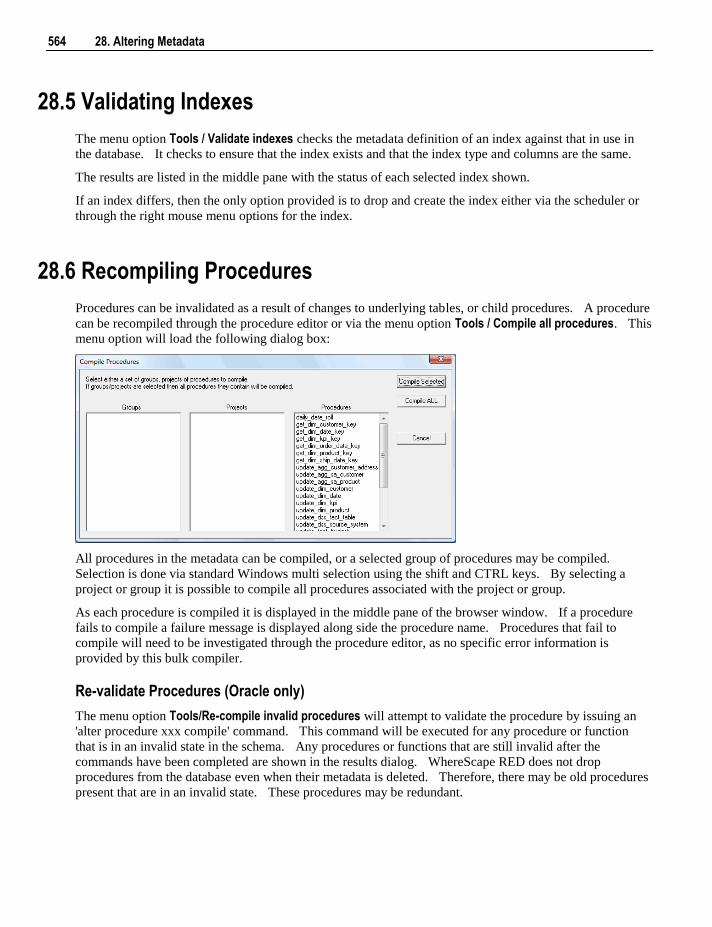
564 28. Altering Metadata
28.5 Validating Indexes
The menu option Tools / Validate indexes checks the metadata definition of an index against that in use in
the database. It checks to ensure that the index exists and that the index type and columns are the same.
The results are listed in the middle pane with the status of each selected index shown.
If an index differs, then the only option provided is to drop and create the index either via the scheduler or
through the right mouse menu options for the index.
28.6 Recompiling Procedures
Procedures can be invalidated as a result of changes to underlying tables, or child procedures. A procedure
can be recompiled through the procedure editor or via the menu option Tools / Compile all procedures. This
menu option will load the following dialog box:
All procedures in the metadata can be compiled, or a selected group of procedures may be compiled.
Selection is done via standard Windows multi selection using the shift and CTRL keys. By selecting a
project or group it is possible to compile all procedures associated with the project or group.
As each procedure is compiled it is displayed in the middle pane of the browser window. If a procedure
fails to compile a failure message is displayed along side the procedure name. Procedures that fail to
compile will need to be investigated through the procedure editor, as no specific error information is
provided by this bulk compiler.
Re-validate Procedures (Oracle only)
The menu option Tools/Re-compile invalid procedures will attempt to validate the procedure by issuing an
'alter procedure xxx compile' command. This command will be executed for any procedure or function
that is in an invalid state in the schema. Any procedures or functions that are still invalid after the
commands have been completed are shown in the results dialog. WhereScape RED does not drop
procedures from the database even when their metadata is deleted. Therefore, there may be old procedures
present that are in an invalid state. These procedures may be redundant.
Chapter 29 29. Callable Procedures 565
In This Chapter
29.1 Introduction to Callable Procedures .................................... 566
29.2 Terminology ........................................................................ 567
29.3 Common Parameters ........................................................... 568
29.4 Ws_Api_Glossary ............................................................... 568
29.5 Ws_Connect_Replace ......................................................... 571
29.6 Ws_Job_Clear_Archive ...................................................... 576
29.7 Ws_Job_Clear_Logs ........................................................... 581
29.8 Ws_Job_Clear_Logs_By_Date ........................................... 585
29.9 Ws_Job_Create ................................................................... 589
29.10 Ws_Job_CreateWait.......................................................... 595
29.11 Ws_Job_Dependency ........................................................ 601
29.12 Ws_Job_Release ............................................................... 607
29.13 Ws_Job_Restart ................................................................ 612
29.14 Ws_Job_Schedule ............................................................. 617
29.15 Ws_Job_Status .................................................................. 622
29.16 Ws_Load_Change ............................................................. 629
29.17 Ws_Maintain_Indexes ...................................................... 634
29.18 Ws_Sched_Status .............................................................. 638
29.19 Ws_Version_Clear ............................................................ 640
29.20 WsParameterRead ............................................................. 644
29.21 WsParameterReadG .......................................................... 647
29.22 WsParameterReadJ ........................................................... 650
29.23 WsParameterWrite ............................................................ 653
29.24 WsWrkAudit ..................................................................... 656
29.25 WsWrkAuditBulk ............................................................. 659
29.26 WsWrkError ...................................................................... 663
29.27 WsWrkErrorBulk .............................................................. 666
29.28 WsWrkTask ...................................................................... 671
C H A P T E R 2 9
29. Callable Procedures
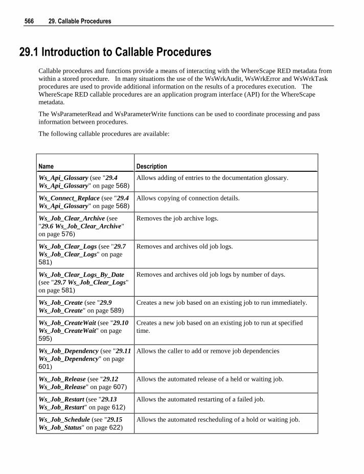
566 29. Callable Procedures
29.1 Introduction to Callable Procedures
Callable procedures and functions provide a means of interacting with the WhereScape RED metadata from
within a stored procedure. In many situations the use of the WsWrkAudit, WsWrkError and WsWrkTask
procedures are used to provide additional information on the results of a procedures execution. The
WhereScape RED callable procedures are an application program interface (API) for the WhereScape
metadata.
The WsParameterRead and WsParameterWrite functions can be used to coordinate processing and pass
information between procedures.
The following callable procedures are available:
Name Description
Ws_Api_Glossary (see "29.4
Ws_Api_Glossary" on page 568)
Allows adding of entries to the documentation glossary.
Ws_Connect_Replace (see "29.4
Ws_Api_Glossary" on page 568)
Allows copying of connection details.
Ws_Job_Clear_Archive (see
"29.6 Ws_Job_Clear_Archive"
on page 576)
Removes the job archive logs.
Ws_Job_Clear_Logs (see "29.7
Ws_Job_Clear_Logs" on page
581)
Removes and archives old job logs.
Ws_Job_Clear_Logs_By_Date (see "29.7 Ws_Job_Clear_Logs"
on page 581)
Removes and archives old job logs by number of days.
Ws_Job_Create (see "29.9
Ws_Job_Create" on page 589)
Creates a new job based on an existing job to run immediately.
Ws_Job_CreateWait (see "29.10
Ws_Job_CreateWait" on page
595)
Creates a new job based on an existing job to run at specified
time.
Ws_Job_Dependency (see "29.11
Ws_Job_Dependency" on page
601)
Allows the caller to add or remove job dependencies
Ws_Job_Release (see "29.12
Ws_Job_Release" on page 607)
Allows the automated release of a held or waiting job.
Ws_Job_Restart (see "29.13
Ws_Job_Restart" on page 612)
Allows the automated restarting of a failed job.
Ws_Job_Schedule (see "29.15
Ws_Job_Status" on page 622)
Allows the automated rescheduling of a hold or waiting job.
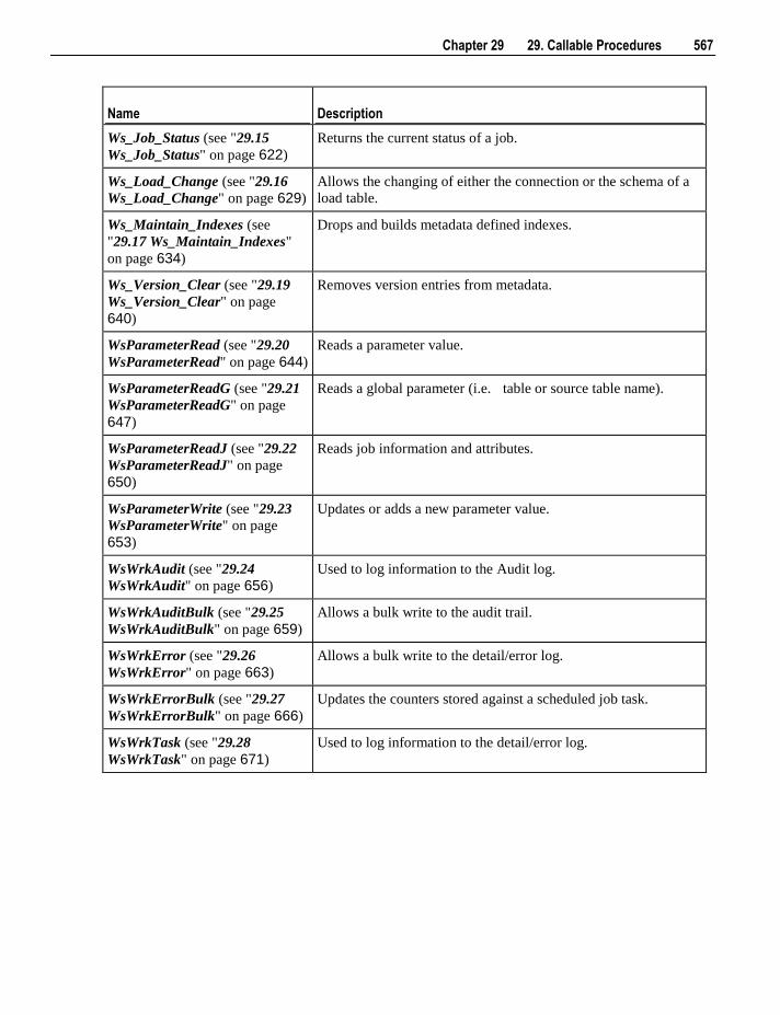
Chapter 29 29. Callable Procedures 567
Name Description
Ws_Job_Status (see "29.15
Ws_Job_Status" on page 622)
Returns the current status of a job.
Ws_Load_Change (see "29.16
Ws_Load_Change" on page 629)
Allows the changing of either the connection or the schema of a
load table.
Ws_Maintain_Indexes (see
"29.17 Ws_Maintain_Indexes"
on page 634)
Drops and builds metadata defined indexes.
Ws_Version_Clear (see "29.19
Ws_Version_Clear" on page
640)
Removes version entries from metadata.
WsParameterRead (see "29.20
WsParameterRead" on page 644)
Reads a parameter value.
WsParameterReadG (see "29.21
WsParameterReadG" on page
647)
Reads a global parameter (i.e. table or source table name).
WsParameterReadJ (see "29.22
WsParameterReadJ" on page
650)
Reads job information and attributes.
WsParameterWrite (see "29.23
WsParameterWrite" on page
653)
Updates or adds a new parameter value.
WsWrkAudit (see "29.24
WsWrkAudit" on page 656)
Used to log information to the Audit log.
WsWrkAuditBulk (see "29.25
WsWrkAuditBulk" on page 659)
Allows a bulk write to the audit trail.
WsWrkError (see "29.26
WsWrkError" on page 663)
Allows a bulk write to the detail/error log.
WsWrkErrorBulk (see "29.27
WsWrkErrorBulk" on page 666)
Updates the counters stored against a scheduled job task.
WsWrkTask (see "29.28
WsWrkTask" on page 671)
Used to log information to the detail/error log.
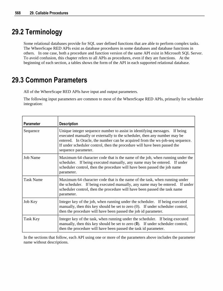
568 29. Callable Procedures
29.2 Terminology
Some relational databases provide for SQL user defined functions that are able to perform complex tasks.
The WhereScape RED APIs exist as database procedures in some databases and database functions in
others. In one case, both a procedure and function version of the same API exist in Microsoft SQL Server.
To avoid confusion, this chapter refers to all APIs as procedures, even if they are functions. At the
beginning of each section, a tables shows the form of the API in each supported relational database.
29.3 Common Parameters
All of the WhereScape RED APIs have input and output parameters.
The following input parameters are common to most of the WhereScape RED APIs, primarily for scheduler
integration:
Parameter Description
Sequence Unique integer sequence number to assist in identifying messages. If being
executed manually or externally to the scheduler, then any number may be
entered. In Oracle, the number can be acquired from the ws-job-seq sequence.
If under scheduler control, then the procedure will have been passed the
sequence parameter.
Job Name Maximum 64 character code that is the name of the job, when running under the
scheduler. If being executed manually, any name may be entered. If under
scheduler control, then the procedure will have been passed the job name
parameter.
Task Name Maximum 64 character code that is the name of the task, when running under
the scheduler. If being executed manually, any name may be entered. If under
scheduler control, then the procedure will have been passed the task name
parameter.
Job Key Integer key of the job, when running under the scheduler. If being executed
manually, then this key should be set to zero (0). If under scheduler control,
then the procedure will have been passed the job id parameter.
Task Key Integer key of the task, when running under the scheduler. If being executed
manually, then this key should be set to zero (0). If under scheduler control,
then the procedure will have been passed the task id parameter.
In the sections that follow, each API using one or more of the parameters above includes the parameter
name without descriptions.
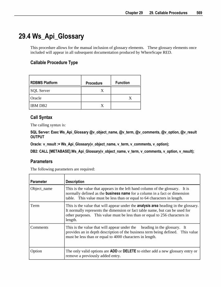
Chapter 29 29. Callable Procedures 569
29.4 Ws_Api_Glossary
This procedure allows for the manual inclusion of glossary elements. These glossary elements once
included will appear in all subsequent documentation produced by WhereScape RED.
Callable Procedure Type
RDBMS Platform Procedure Function
SQL Server X
Oracle X
IBM DB2 X
Call Syntax
The calling syntax is:
SQL Server: Exec Ws_Api_Glossary @v_object_name, @v_term, @v_comments, @v_option, @v_result OUTPUT
Oracle: v_result := Ws_Api_Glossary(v_object_name, v_term, v_comments, v_option);
DB2: CALL [METABASE].Ws_Api_Glossary(v_object_name, v_term, v_comments, v_option, v_result);
Parameters
The following parameters are required:
Parameter Description
Object_name This is the value that appears in the left hand column of the glossary. It is
normally defined as the business name for a column in a fact or dimension
table. This value must be less than or equal to 64 characters in length.
Term This is the value that will appear under the analysis area heading in the glossary.
It normally represents the dimension or fact table name, but can be used for
other purposes. This value must be less than or equal to 256 characters in
length.
Comments This is the value that will appear under the heading in the glossary. It
provides an in depth description of the business term being defined. This value
must be less than or equal to 4000 characters in length.
Option The only valid options are ADD or DELETE to either add a new glossary entry or
remove a previously added entry.
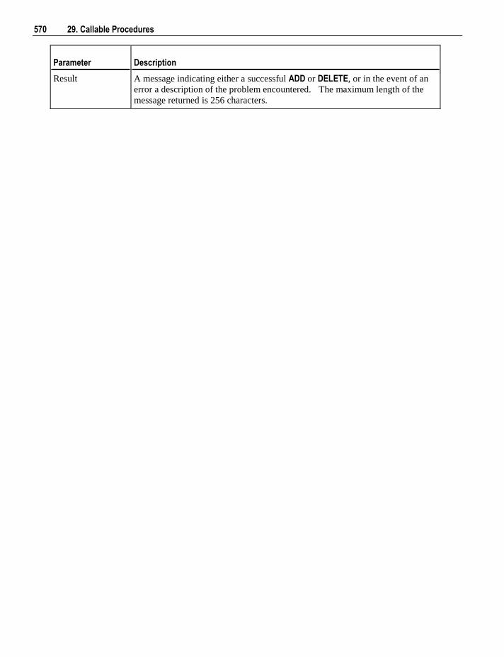
570 29. Callable Procedures
Parameter Description
Result A message indicating either a successful ADD or DELETE, or in the event of an
error a description of the problem encountered. The maximum length of the
message returned is 256 characters.
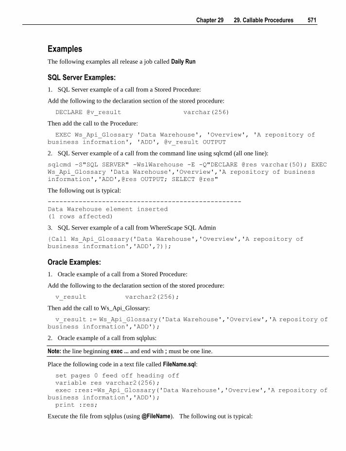
Chapter 29 29. Callable Procedures 571
Examples
The following examples all release a job called Daily Run
SQL Server Examples:
1. SQL Server example of a call from a Stored Procedure:
Add the following to the declaration section of the stored procedure:
DECLARE @v_result varchar(256)
Then add the call to the Procedure:
EXEC Ws_Api_Glossary 'Data Warehouse', 'Overview', 'A repository of
business information', 'ADD', @v_result OUTPUT
2. SQL Server example of a call from the command line using sqlcmd (all one line):
sqlcmd -S"SQL SERVER" -WslWarehouse -E -Q"DECLARE @res varchar(50); EXEC
Ws_Api_Glossary 'Data Warehouse','Overview','A repository of business
information','ADD',@res OUTPUT; SELECT @res"
The following out is typical:
--------------------------------------------------
Data Warehouse element inserted
(1 rows affected)
3. SQL Server example of a call from WhereScape SQL Admin
{Call Ws_Api_Glossary('Data Warehouse','Overview','A repository of
business information','ADD',?)};
Oracle Examples:
1. Oracle example of a call from a Stored Procedure:
Add the following to the declaration section of the stored procedure:
v_result varchar2(256);
Then add the call to Ws_Api_Glossary:
v_result := Ws_Api_Glossary('Data Warehouse','Overview','A repository of
business information','ADD');
2. Oracle example of a call from sqlplus:
Note: the line beginning exec ... and end with ; must be one line.
Place the following code in a text file called FileName.sql:
set pages 0 feed off heading off
variable res varchar2(256);
exec :res:=Ws_Api_Glossary('Data Warehouse','Overview','A repository of
business information','ADD');
print :res;
Execute the file from sqlplus (using @FileName). The following out is typical:
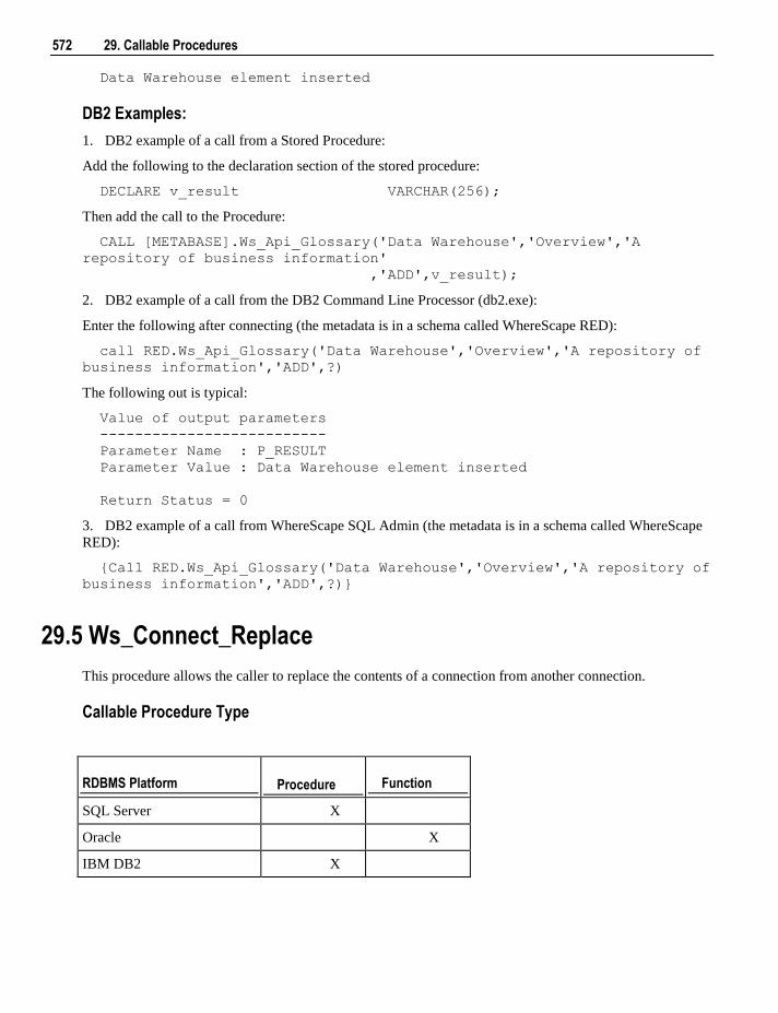
572 29. Callable Procedures
Data Warehouse element inserted
DB2 Examples:
1. DB2 example of a call from a Stored Procedure:
Add the following to the declaration section of the stored procedure:
DECLARE v_result VARCHAR(256);
Then add the call to the Procedure:
CALL [METABASE].Ws_Api_Glossary('Data Warehouse','Overview','A
repository of business information'
,'ADD',v_result);
2. DB2 example of a call from the DB2 Command Line Processor (db2.exe):
Enter the following after connecting (the metadata is in a schema called WhereScape RED):
call RED.Ws_Api_Glossary('Data Warehouse','Overview','A repository of
business information','ADD',?)
The following out is typical:
Value of output parameters
--------------------------
Parameter Name : P_RESULT
Parameter Value : Data Warehouse element inserted
Return Status = 0
3. DB2 example of a call from WhereScape SQL Admin (the metadata is in a schema called WhereScape
RED):
{Call RED.Ws_Api_Glossary('Data Warehouse','Overview','A repository of
business information','ADD',?)}
29.5 Ws_Connect_Replace
This procedure allows the caller to replace the contents of a connection from another connection.
Callable Procedure Type
RDBMS Platform Procedure Function
SQL Server X
Oracle X
IBM DB2 X
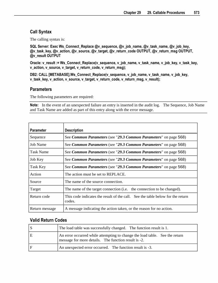
Chapter 29 29. Callable Procedures 573
Call Syntax
The calling syntax is:
SQL Server: Exec Ws_Connect_Replace @v_sequence, @v_job_name, @v_task_name, @v_job_key, @v_task_key, @v_action, @v_source, @v_target, @v_return_code OUTPUT, @v_return_msg OUTPUT, @v_result OUTPUT
Oracle: v_result := Ws_Connect_Replace(v_sequence, v_job_name, v_task_name, v_job_key, v_task_key, v_action, v_source, v_target, v_return_code, v_return_msg);
DB2: CALL [METABASE].Ws_Connect_Replace(v_sequence, v_job_name, v_task_name, v_job_key, v_task_key, v_action, v_source, v_target, v_return_code, v_return_msg, v_result);
Parameters
The following parameters are required:
Note: In the event of an unexpected failure an entry is inserted in the audit log. The Sequence, Job Name
and Task Name are added as part of this entry along with the error message.
Parameter Description
Sequence See Common Parameters (see "29.3 Common Parameters" on page 568)
Job Name See Common Parameters (see "29.3 Common Parameters" on page 568)
Task Name See Common Parameters (see "29.3 Common Parameters" on page 568)
Job Key See Common Parameters (see "29.3 Common Parameters" on page 568)
Task Key See Common Parameters (see "29.3 Common Parameters" on page 568)
Action The action must be set to REPLACE.
Source The name of the source connection.
Target The name of the target connection (i.e. the connection to be changed).
Return code This code indicates the result of the call. See the table below for the return
codes.
Return message A message indicating the action taken, or the reason for no action.
Valid Return Codes
S The load table was successfully changed. The function result is 1.
E An error occurred while attempting to change the load table. See the return
message for more details. The function result is -2.
F An unexpected error occurred. The function result is -3.

574 29. Callable Procedures
Returned result
1 will be returned if the function changed the load table.
–2 will be returned if the load table could not be changed.
–3 will be returned if an unhandled error occurred.
Examples
The following examples all release a job called Daily Run
SQL Server Examples:
1. SQL Server example of a call from a Stored Procedure:
Add the following to the declaration section of the stored procedure:
DECLARE @v_result integer
DECLARE @v_return_code varchar(1)
DECLARE @v_return_msg varchar(256)
Then add the call to the procedure:
EXEC Ws_Connect_Replace @p_sequence, @p_job_name, @p_task_name,
@p_job_id, @p_task_id
, 'REPLACE', 'CONN_TEST2', 'CONN_TEST1'
, @v_return_code OUTPUT, @v_return_msg OUTPUT, @v_result
OUTPUT
Perhaps add a check of the result:
IF @v_result <> 1
BEGIN
SET @p_status =@v_result
SET @p_return_msg = 'Failed to replace connection details. Return Code
was ' +@v_return_code
SET @p_return_msg = @p_return_msg + '. ' + RTRIM(@v_return_msg)
END
2. SQL Server example of a call from the command line using sqlcmd (all one line):
sqlcmd -S"SQL SERVER" -WslWarehouse -E -Q"DECLARE @RES integer;DECLARE @RET
varchar(1);DECLARE @MSG varchar(77);EXEC Ws_Connect_Replace 0,'Change
Conn','Conn',0,0,'REPLACE','CONN_TEST2','CONN_TEST1',@RET OUTPUT,@MSG
OUTPUT,@RES OUTPUT; SELECT @RET,@MSG"
The following out is typical:
-
------------------------------------------------------------------------
-----
S Connection information for CONN_TEST1 replaced from CONN_TEST2
(1 rows affected)
3. SQL Server example of a call from WhereScape SQL Admin
{Call Ws_Connect_Replace(0,'Change
Conn','Conn',0,0,'REPLACE','CONN_TEST2','CONN_TEST1',?,?,?)};
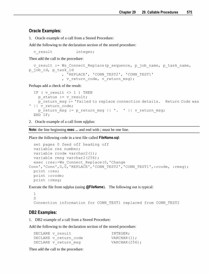
Chapter 29 29. Callable Procedures 575
Oracle Examples:
1. Oracle example of a call from a Stored Procedure:
Add the following to the declaration section of the stored procedure:
v_result integer;
Then add the call to the procedure:
v_result := Ws_Connect_Replace(p_sequence, p_job_name, p_task_name,
p_job_id, p_task_id
, 'REPLACE', 'CONN_TEST2', 'CONN_TEST1'
, v_return_code, v_return_msg);
Perhaps add a check of the result:
IF ( v_result <> 1 ) THEN
p_status := v_result;
p_return_msg := 'Failed to replace connection details. Return Code was
' || v_return_code;
p_return_msg := p_return_msg || '. ' || v_return_msg;
END IF;
2. Oracle example of a call from sqlplus:
Note: the line beginning exec ... and end with ; must be one line.
Place the following code in a text file called FileName.sql:
set pages 0 feed off heading off
variable res number;
variable rcode varchar2(1);
variable rmsg varchar2(256);
exec :res:=Ws_Connect_Replace(0,'Change
Conn','Conn',0,0,'REPLACE','CONN_TEST2','CONN_TEST1',:rcode, :rmsg);
print :res;
print :rcode;
print :rmsg;
Execute the file from sqlplus (using @FileName). The following out is typical:
1
S
Connection information for CONN_TEST1 replaced from CONN_TEST2
DB2 Examples:
1. DB2 example of a call from a Stored Procedure:
Add the following to the declaration section of the stored procedure:
DECLARE v_result INTEGER;
DECLARE v_return_code VARCHAR(1);
DECLARE v_return_msg VARCHAR(256);
Then add the call to the procedure:
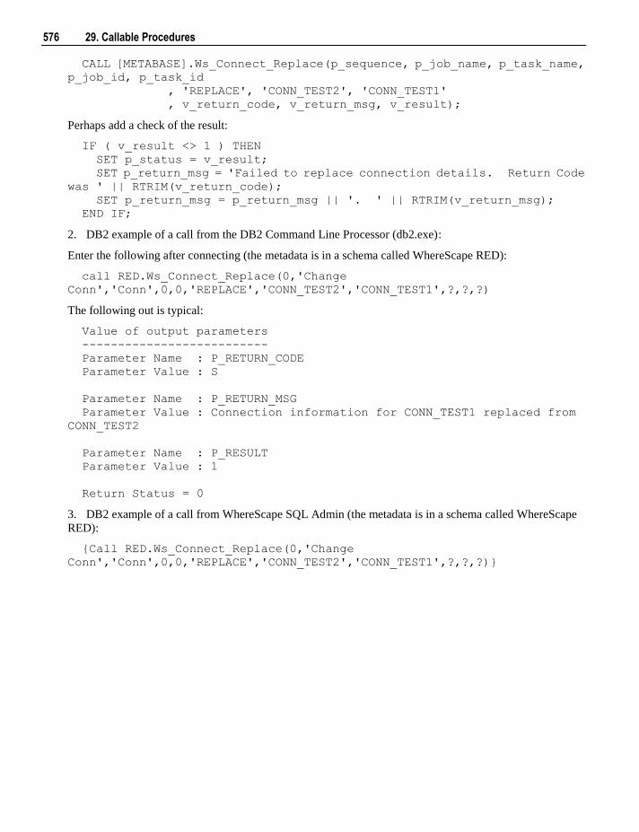
576 29. Callable Procedures
CALL [METABASE].Ws_Connect_Replace(p_sequence, p_job_name, p_task_name,
p_job_id, p_task_id
, 'REPLACE', 'CONN_TEST2', 'CONN_TEST1'
, v_return_code, v_return_msg, v_result);
Perhaps add a check of the result:
IF ( v_result <> 1 ) THEN
SET p_status = v_result;
SET p_return_msg = 'Failed to replace connection details. Return Code
was ' || RTRIM(v_return_code);
SET p_return_msg = p_return_msg || '. ' || RTRIM(v_return_msg);
END IF;
2. DB2 example of a call from the DB2 Command Line Processor (db2.exe):
Enter the following after connecting (the metadata is in a schema called WhereScape RED):
call RED.Ws_Connect_Replace(0,'Change
Conn','Conn',0,0,'REPLACE','CONN_TEST2','CONN_TEST1',?,?,?)
The following out is typical:
Value of output parameters
--------------------------
Parameter Name : P_RETURN_CODE
Parameter Value : S
Parameter Name : P_RETURN_MSG
Parameter Value : Connection information for CONN_TEST1 replaced from
CONN_TEST2
Parameter Name : P_RESULT
Parameter Value : 1
Return Status = 0
3. DB2 example of a call from WhereScape SQL Admin (the metadata is in a schema called WhereScape
RED):
{Call RED.Ws_Connect_Replace(0,'Change
Conn','Conn',0,0,'REPLACE','CONN_TEST2','CONN_TEST1',?,?,?)}
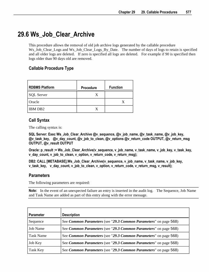
Chapter 29 29. Callable Procedures 577
29.6 Ws_Job_Clear_Archive
This procedure allows the removal of old job archive logs generated by the callable procedure
Ws_Job_Clear_Logs and Ws_Job_Clear_Logs_By_Date. The number of days of logs to retain is specified
and all older logs are deleted. If zero is specified all logs are deleted. For example if 90 is specified then
logs older than 90 days old are removed.
Callable Procedure Type
RDBMS Platform Procedure Function
SQL Server X
Oracle X
IBM DB2 X
Call Syntax
The calling syntax is:
SQL Server: Exec Ws_Job_Clear_Archive @v_sequence, @v_job_name, @v_task_name, @v_job_key, @v_task_key, @v_day_count, @v_job_to_clean, @v_options @v_return_code OUTPUT, @v_return_msg OUTPUT, @v_result OUTPUT
Oracle: p_result := Ws_Job_Clear_Archive(v_sequence, v_job_name, v_task_name, v_job_key, v_task_key, v_day_count, v_job_to_clean, v_option, v_return_code, v_return_msg);
DB2: CALL [METABASE].Ws_Job_Clear_Archive(v_sequence, v_job_name, v_task_name, v_job_key, v_task_key, v_day_count, v_job_to_clean, v_option, v_return_code, v_return_msg, v_result);
Parameters
The following parameters are required:
Note: In the event of an unexpected failure an entry is inserted in the audit log. The Sequence, Job Name
and Task Name are added as part of this entry along with the error message.
Parameter Description
Sequence See Common Parameters (see "29.3 Common Parameters" on page 568)
Job Name See Common Parameters (see "29.3 Common Parameters" on page 568)
Task Name See Common Parameters (see "29.3 Common Parameters" on page 568)
Job Key See Common Parameters (see "29.3 Common Parameters" on page 568)
Task Key See Common Parameters (see "29.3 Common Parameters" on page 568)
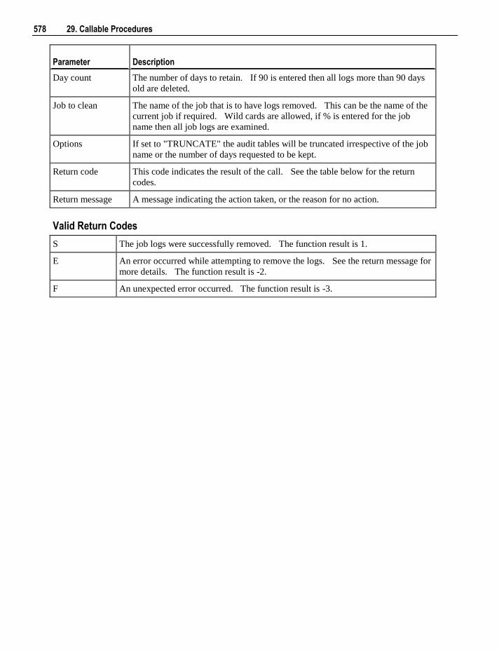
578 29. Callable Procedures
Parameter Description
Day count The number of days to retain. If 90 is entered then all logs more than 90 days
old are deleted.
Job to clean The name of the job that is to have logs removed. This can be the name of the
current job if required. Wild cards are allowed, if % is entered for the job
name then all job logs are examined.
Options If set to "TRUNCATE" the audit tables will be truncated irrespective of the job
name or the number of days requested to be kept.
Return code This code indicates the result of the call. See the table below for the return
codes.
Return message A message indicating the action taken, or the reason for no action.
Valid Return Codes
S The job logs were successfully removed. The function result is 1.
E An error occurred while attempting to remove the logs. See the return message for
more details. The function result is -2.
F An unexpected error occurred. The function result is -3.
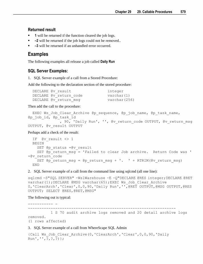
Chapter 29 29. Callable Procedures 579
Returned result
1 will be returned if the function cleared the job logs.
–2 will be returned if the job logs could not be removed..
–3 will be returned if an unhandled error occurred.
Examples
The following examples all release a job called Daily Run
SQL Server Examples:
1. SQL Server example of a call from a Stored Procedure:
Add the following to the declaration section of the stored procedure:
DECLARE @v_result integer
DECLARE @v_return_code varchar(1)
DECLARE @v_return_msg varchar(256)
Then add the call to the procedure:
EXEC Ws_Job_Clear_Archive @p_sequence, @p_job_name, @p_task_name,
@p_job_id, @p_task_id
, 90, 'Daily Run', '', @v_return_code OUTPUT, @v_return_msg
OUTPUT, @v_result OUTPUT
Perhaps add a check of the result:
IF @v_result <> 1
BEGIN
SET @p_status =@v_result
SET @p_return_msg = 'Failed to clear Job archive. Return Code was '
+@v_return_code
SET @p_return_msg = @p_return_msg + '. ' + RTRIM(@v_return_msg)
END
2. SQL Server example of a call from the command line using sqlcmd (all one line):
sqlcmd -S"SQL SERVER" -WslWarehouse -E -Q"DECLARE @RES integer;DECLARE @RET
varchar(1);DECLARE @MSG varchar(65);EXEC Ws_Job_Clear_Archive
0,'ClearArch','Clear',0,0,90,'Daily Run','',@RET OUTPUT,@MSG OUTPUT,@RES
OUTPUT; SELECT @RES,@RET,@MSG"
The following out is typical:
----------- -
-----------------------------------------------------------------
1 S 70 audit archive logs removed and 20 detail archive logs
removed.
(1 rows affected)
3. SQL Server example of a call from WhereScape SQL Admin
{Call Ws_Job_Clear_Archive(0,'ClearArch','Clear',0,0,90,'Daily
Run','',?,?,?)};
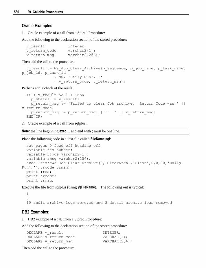
580 29. Callable Procedures
Oracle Examples:
1. Oracle example of a call from a Stored Procedure:
Add the following to the declaration section of the stored procedure:
v_result integer;
v_return_code varchar2(1);
v_return_msg varchar2(256);
Then add the call to the procedure:
v_result := Ws_Job_Clear_Archive(p_sequence, p_job_name, p_task_name,
p_job_id, p_task_id
, 90, 'Daily Run', ''
, v_return_code, v_return_msg);
Perhaps add a check of the result:
IF ( v_result <> 1 ) THEN
p_status := v_result;
p_return_msg := 'Failed to clear Job archive. Return Code was ' ||
v_return_code;
p_return_msg := p_return_msg || '. ' || v_return_msg;
END IF;
2. Oracle example of a call from sqlplus:
Note: the line beginning exec ... and end with ; must be one line.
Place the following code in a text file called FileName.sql:
set pages 0 feed off heading off
variable res number;
variable rcode varchar2(1);
variable rmsg varchar2(256);
exec :res:=Ws_Job_Clear_Archive(0,'ClearArch','Clear',0,0,90,'Daily
Run','',:rcode,:rmsg);
print :res;
print :rcode;
print :rmsg;
Execute the file from sqlplus (using @FileName). The following out is typical:
1
S
10 audit archive logs removed and 3 detail archive logs removed.
DB2 Examples:
1. DB2 example of a call from a Stored Procedure:
Add the following to the declaration section of the stored procedure:
DECLARE v_result INTEGER;
DECLARE v_return_code VARCHAR(1);
DECLARE v_return_msg VARCHAR(256);
Then add the call to the procedure:
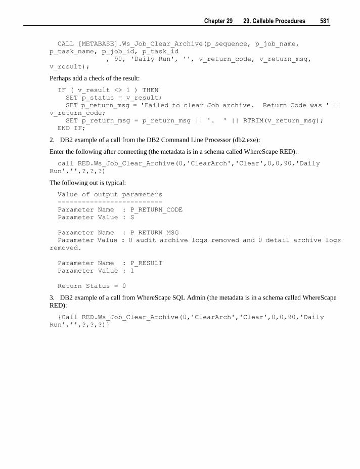
Chapter 29 29. Callable Procedures 581
CALL [METABASE].Ws_Job_Clear_Archive(p_sequence, p_job_name,
p_task_name, p_job_id, p_task_id
, 90, 'Daily Run', '', v_return_code, v_return_msg,
v_result);
Perhaps add a check of the result:
IF ( v_result <> 1 ) THEN
SET p_status = v_result;
SET p_return_msg = 'Failed to clear Job archive. Return Code was ' ||
v_return_code;
SET p_return_msg = p_return_msg || '. ' || RTRIM(v_return_msg);
END IF;
2. DB2 example of a call from the DB2 Command Line Processor (db2.exe):
Enter the following after connecting (the metadata is in a schema called WhereScape RED):
call RED.Ws_Job_Clear_Archive(0,'ClearArch','Clear',0,0,90,'Daily
Run','',?,?,?)
The following out is typical:
Value of output parameters
--------------------------
Parameter Name : P_RETURN_CODE
Parameter Value : S
Parameter Name : P_RETURN_MSG
Parameter Value : 0 audit archive logs removed and 0 detail archive logs
removed.
Parameter Name : P_RESULT
Parameter Value : 1
Return Status = 0
3. DB2 example of a call from WhereScape SQL Admin (the metadata is in a schema called WhereScape
RED):
{Call RED.Ws_Job_Clear_Archive(0,'ClearArch','Clear',0,0,90,'Daily
Run','',?,?,?)}
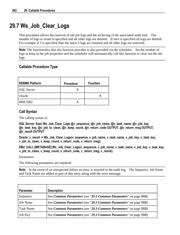
582 29. Callable Procedures
29.7 Ws_Job_Clear_Logs
This procedure allows the removal of old job logs and the archiving of the associated audit trail. The
number of logs to retain is specified and all older logs are deleted. If zero is specified all logs are deleted.
For example if 3 is specified then the latest 3 logs are retained and all older logs are removed.
Note: The functionality that this function provides is also provided via the scheduler. Set the number of
logs to keep in the job properties and the scheduler will automatically call this function to clear out the old
logs.
Callable Procedure Type
RDBMS Platform Procedure Function
SQL Server X
Oracle X
IBM DB2 X
Call Syntax
The calling syntax is:
SQL Server: Exec Ws_Job_Clear_Logs @v_sequence, @v_job_name, @v_task_name, @v_job_key, @v_task_key, @v_job_to_clean, @v_keep_count, @v_return_code OUTPUT, @v_return_msg OUTPUT, @v_result OUTPUT
Oracle: v_result := Ws_Job_Clear_Logs(v_sequence, v_job_name, v_task_name, v_job_key, v_task_key, v_job_to_clean, v_keep_count, v_return_code, v_return_msg);
DB2: CALL [METABASE].Ws_Job_Clear_Logs(v_sequence, v_job_name, v_task_name, v_job_key, v_task_key, v_job_to_clean, v_keep_count, v_return_code, v_return_msg, v_result);
Parameters
The following parameters are required:
Note: In the event of an unexpected failure an entry is inserted in the audit log. The Sequence, Job Name
and Task Name are added as part of this entry along with the error message.
Parameter Description
Sequence See Common Parameters (see "29.3 Common Parameters" on page 568)
Job Name See Common Parameters (see "29.3 Common Parameters" on page 568)
Task Name See Common Parameters (see "29.3 Common Parameters" on page 568)
Job Key See Common Parameters (see "29.3 Common Parameters" on page 568)
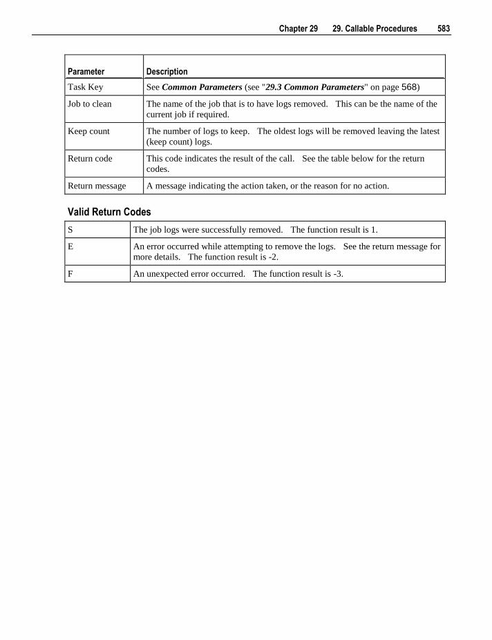
Chapter 29 29. Callable Procedures 583
Parameter Description
Task Key See Common Parameters (see "29.3 Common Parameters" on page 568)
Job to clean The name of the job that is to have logs removed. This can be the name of the
current job if required.
Keep count The number of logs to keep. The oldest logs will be removed leaving the latest
(keep count) logs.
Return code This code indicates the result of the call. See the table below for the return
codes.
Return message A message indicating the action taken, or the reason for no action.
Valid Return Codes
S The job logs were successfully removed. The function result is 1.
E An error occurred while attempting to remove the logs. See the return message for
more details. The function result is -2.
F An unexpected error occurred. The function result is -3.
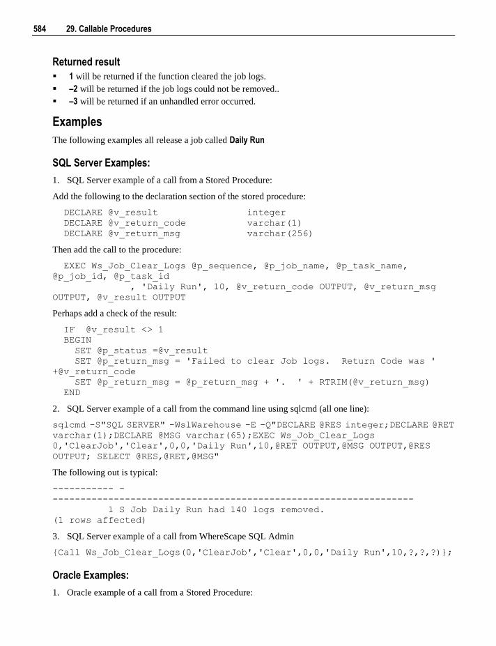
584 29. Callable Procedures
Returned result
1 will be returned if the function cleared the job logs.
–2 will be returned if the job logs could not be removed..
–3 will be returned if an unhandled error occurred.
Examples
The following examples all release a job called Daily Run
SQL Server Examples:
1. SQL Server example of a call from a Stored Procedure:
Add the following to the declaration section of the stored procedure:
DECLARE @v_result integer
DECLARE @v_return_code varchar(1)
DECLARE @v_return_msg varchar(256)
Then add the call to the procedure:
EXEC Ws_Job_Clear_Logs @p_sequence, @p_job_name, @p_task_name,
@p_job_id, @p_task_id
, 'Daily Run', 10, @v_return_code OUTPUT, @v_return_msg
OUTPUT, @v_result OUTPUT
Perhaps add a check of the result:
IF @v_result <> 1
BEGIN
SET @p_status =@v_result
SET @p_return_msg = 'Failed to clear Job logs. Return Code was '
+@v_return_code
SET @p_return_msg = @p_return_msg + '. ' + RTRIM(@v_return_msg)
END
2. SQL Server example of a call from the command line using sqlcmd (all one line):
sqlcmd -S"SQL SERVER" -WslWarehouse -E -Q"DECLARE @RES integer;DECLARE @RET
varchar(1);DECLARE @MSG varchar(65);EXEC Ws_Job_Clear_Logs
0,'ClearJob','Clear',0,0,'Daily Run',10,@RET OUTPUT,@MSG OUTPUT,@RES
OUTPUT; SELECT @RES,@RET,@MSG"
The following out is typical:
----------- -
-----------------------------------------------------------------
1 S Job Daily Run had 140 logs removed.
(1 rows affected)
3. SQL Server example of a call from WhereScape SQL Admin
{Call Ws_Job_Clear_Logs(0,'ClearJob','Clear',0,0,'Daily Run',10,?,?,?)};
Oracle Examples:
1. Oracle example of a call from a Stored Procedure:
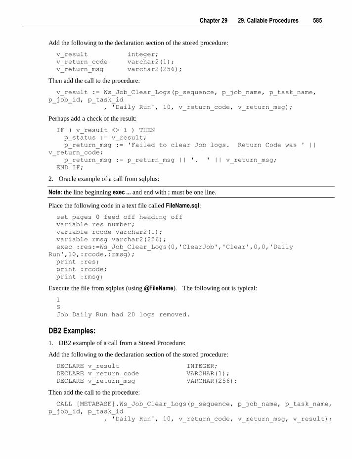
Chapter 29 29. Callable Procedures 585
Add the following to the declaration section of the stored procedure:
v_result integer;
v_return_code varchar2(1);
v_return_msg varchar2(256);
Then add the call to the procedure:
v_result := Ws_Job_Clear_Logs(p_sequence, p_job_name, p_task_name,
p_job_id, p_task_id
, 'Daily Run', 10, v_return_code, v_return_msg);
Perhaps add a check of the result:
IF ( v_result <> 1 ) THEN
p_status := v_result;
p_return_msg := 'Failed to clear Job logs. Return Code was ' ||
v_return_code;
p_return_msg := p_return_msg || '. ' || v_return_msg;
END IF;
2. Oracle example of a call from sqlplus:
Note: the line beginning exec ... and end with ; must be one line.
Place the following code in a text file called FileName.sql:
set pages 0 feed off heading off
variable res number;
variable rcode varchar2(1);
variable rmsg varchar2(256);
exec :res:=Ws_Job_Clear_Logs(0,'ClearJob','Clear',0,0,'Daily
Run',10,:rcode,:rmsg);
print :res;
print :rcode;
print :rmsg;
Execute the file from sqlplus (using @FileName). The following out is typical:
1
S
Job Daily Run had 20 logs removed.
DB2 Examples:
1. DB2 example of a call from a Stored Procedure:
Add the following to the declaration section of the stored procedure:
DECLARE v_result INTEGER;
DECLARE v_return_code VARCHAR(1);
DECLARE v_return_msg VARCHAR(256);
Then add the call to the procedure:
CALL [METABASE].Ws_Job_Clear_Logs(p_sequence, p_job_name, p_task_name,
p_job_id, p_task_id
, 'Daily Run', 10, v_return_code, v_return_msg, v_result);
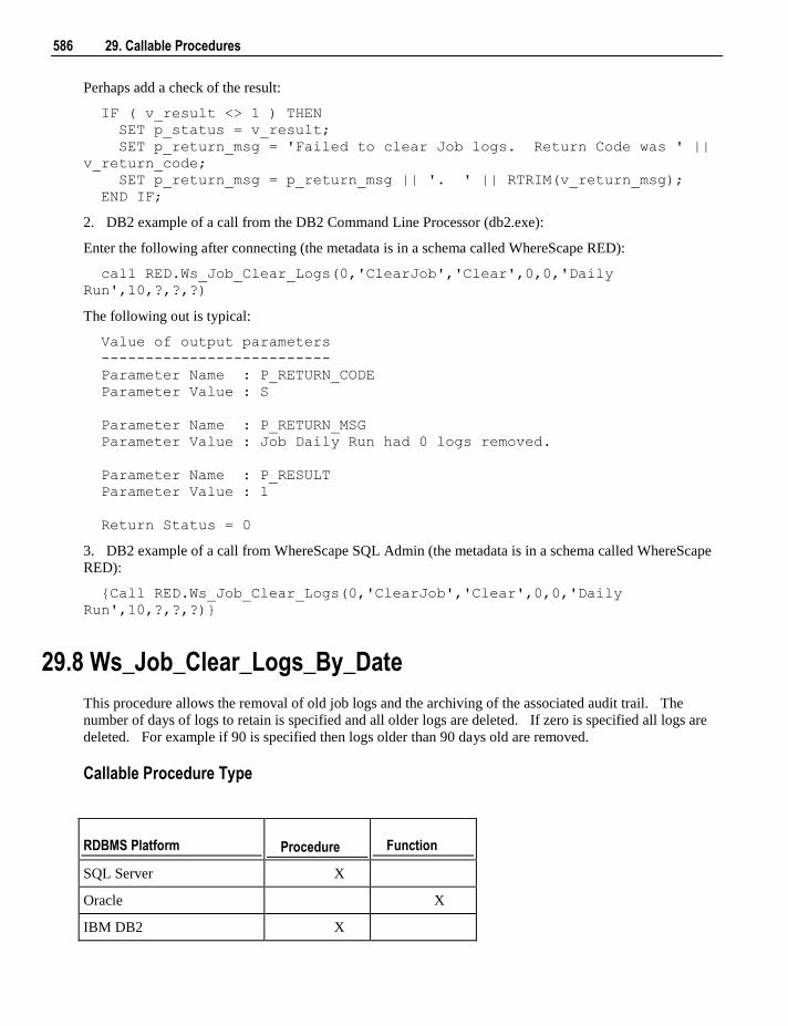
586 29. Callable Procedures
Perhaps add a check of the result:
IF ( v_result <> 1 ) THEN
SET p_status = v_result;
SET p_return_msg = 'Failed to clear Job logs. Return Code was ' ||
v_return_code;
SET p_return_msg = p_return_msg || '. ' || RTRIM(v_return_msg);
END IF;
2. DB2 example of a call from the DB2 Command Line Processor (db2.exe):
Enter the following after connecting (the metadata is in a schema called WhereScape RED):
call RED.Ws_Job_Clear_Logs(0,'ClearJob','Clear',0,0,'Daily
Run',10,?,?,?)
The following out is typical:
Value of output parameters
--------------------------
Parameter Name : P_RETURN_CODE
Parameter Value : S
Parameter Name : P_RETURN_MSG
Parameter Value : Job Daily Run had 0 logs removed.
Parameter Name : P_RESULT
Parameter Value : 1
Return Status = 0
3. DB2 example of a call from WhereScape SQL Admin (the metadata is in a schema called WhereScape
RED):
{Call RED.Ws_Job_Clear_Logs(0,'ClearJob','Clear',0,0,'Daily
Run',10,?,?,?)}
29.8 Ws_Job_Clear_Logs_By_Date
This procedure allows the removal of old job logs and the archiving of the associated audit trail. The
number of days of logs to retain is specified and all older logs are deleted. If zero is specified all logs are
deleted. For example if 90 is specified then logs older than 90 days old are removed.
Callable Procedure Type
RDBMS Platform Procedure Function
SQL Server X
Oracle X
IBM DB2 X
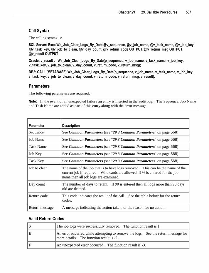
Chapter 29 29. Callable Procedures 587
Call Syntax
The calling syntax is:
SQL Server: Exec Ws_Job_Clear_Logs_By_Date @v_sequence, @v_job_name, @v_task_name, @v_job_key, @v_task_key, @v_job_to_clean, @v_day_count, @v_return_code OUTPUT, @v_return_msg OUTPUT, @v_result OUTPUT
Oracle: v_result := Ws_Job_Clear_Logs_By_Date(p_sequence, v_job_name, v_task_name, v_job_key, v_task_key, v_job_to_clean, v_day_count, v_return_code, v_return_msg);
DB2: CALL [METABASE].Ws_Job_Clear_Logs_By_Date(p_sequence, v_job_name, v_task_name, v_job_key, v_task_key, v_job_to_clean, v_day_count, v_return_code, v_return_msg, v_result);
Parameters
The following parameters are required:
Note: In the event of an unexpected failure an entry is inserted in the audit log. The Sequence, Job Name
and Task Name are added as part of this entry along with the error message.
Parameter Description
Sequence See Common Parameters (see "29.3 Common Parameters" on page 568)
Job Name See Common Parameters (see "29.3 Common Parameters" on page 568)
Task Name See Common Parameters (see "29.3 Common Parameters" on page 568)
Job Key See Common Parameters (see "29.3 Common Parameters" on page 568)
Task Key See Common Parameters (see "29.3 Common Parameters" on page 568)
Job to clean The name of the job that is to have logs removed. This can be the name of the
current job if required. Wild cards are allowed, if % is entered for the job
name then all job logs are examined.
Day count The number of days to retain. If 90 is entered then all logs more than 90 days
old are deleted.
Return code This code indicates the result of the call. See the table below for the return
codes.
Return message A message indicating the action taken, or the reason for no action.
Valid Return Codes
S The job logs were successfully removed. The function result is 1.
E An error occurred while attempting to remove the logs. See the return message for
more details. The function result is -2.
F An unexpected error occurred. The function result is -3.
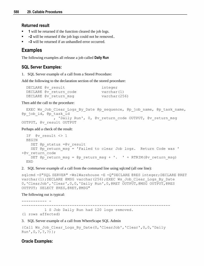
588 29. Callable Procedures
Returned result
1 will be returned if the function cleared the job logs.
–2 will be returned if the job logs could not be removed..
–3 will be returned if an unhandled error occurred.
Examples
The following examples all release a job called Daily Run
SQL Server Examples:
1. SQL Server example of a call from a Stored Procedure:
Add the following to the declaration section of the stored procedure:
DECLARE @v_result integer
DECLARE @v_return_code varchar(1)
DECLARE @v_return_msg varchar(256)
Then add the call to the procedure:
EXEC Ws_Job_Clear_Logs_By_Date @p_sequence, @p_job_name, @p_task_name,
@p_job_id, @p_task_id
, 'Daily Run', 0, @v_return_code OUTPUT, @v_return_msg
OUTPUT, @v_result OUTPUT
Perhaps add a check of the result:
IF @v_result <> 1
BEGIN
SET @p_status =@v_result
SET @p_return_msg = 'Failed to clear Job logs. Return Code was '
+@v_return_code
SET @p_return_msg = @p_return_msg + '. ' + RTRIM(@v_return_msg)
END
2. SQL Server example of a call from the command line using sqlcmd (all one line):
sqlcmd -S"SQL SERVER" -WslWarehouse -E -Q"DECLARE @RES integer;DECLARE @RET
varchar(1);DECLARE @MSG varchar(256);EXEC Ws_Job_Clear_Logs_By_Date
0,'ClearJob','Clear',0,0,'Daily Run',0,@RET OUTPUT,@MSG OUTPUT,@RES
OUTPUT; SELECT @RES,@RET,@MSG"
The following out is typical:
----------- -
-----------------------------------------------------------------
1 S Job Daily Run had 120 logs removed.
(1 rows affected)
3. SQL Server example of a call from WhereScape SQL Admin
{Call Ws_Job_Clear_Logs_By_Date(0,'ClearJob','Clear',0,0,'Daily
Run',0,?,?,?)};
Oracle Examples:
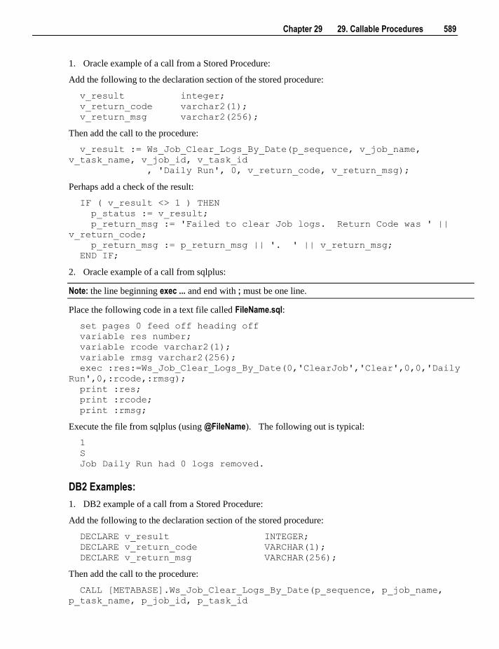
Chapter 29 29. Callable Procedures 589
1. Oracle example of a call from a Stored Procedure:
Add the following to the declaration section of the stored procedure:
v_result integer;
v_return_code varchar2(1);
v_return_msg varchar2(256);
Then add the call to the procedure:
v_result := Ws_Job_Clear_Logs_By_Date(p_sequence, v_job_name,
v_task_name, v_job_id, v_task_id
, 'Daily Run', 0, v_return_code, v_return_msg);
Perhaps add a check of the result:
IF ( v_result <> 1 ) THEN
p_status := v_result;
p_return_msg := 'Failed to clear Job logs. Return Code was ' ||
v_return_code;
p_return_msg := p_return_msg || '. ' || v_return_msg;
END IF;
2. Oracle example of a call from sqlplus:
Note: the line beginning exec ... and end with ; must be one line.
Place the following code in a text file called FileName.sql:
set pages 0 feed off heading off
variable res number;
variable rcode varchar2(1);
variable rmsg varchar2(256);
exec :res:=Ws_Job_Clear_Logs_By_Date(0,'ClearJob','Clear',0,0,'Daily
Run',0,:rcode,:rmsg);
print :res;
print :rcode;
print :rmsg;
Execute the file from sqlplus (using @FileName). The following out is typical:
1
S
Job Daily Run had 0 logs removed.
DB2 Examples:
1. DB2 example of a call from a Stored Procedure:
Add the following to the declaration section of the stored procedure:
DECLARE v_result INTEGER;
DECLARE v_return_code VARCHAR(1);
DECLARE v_return_msg VARCHAR(256);
Then add the call to the procedure:
CALL [METABASE].Ws_Job_Clear_Logs_By_Date(p_sequence, p_job_name,
p_task_name, p_job_id, p_task_id
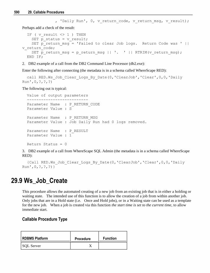
590 29. Callable Procedures
, 'Daily Run', 0, v_return_code, v_return_msg, v_result);
Perhaps add a check of the result:
IF ( v_result <> 1 ) THEN
SET p_status = v_result;
SET p_return_msg = 'Failed to clear Job logs. Return Code was ' ||
v_return_code;
SET p_return_msg = p_return_msg || '. ' || RTRIM(v_return_msg);
END IF;
2. DB2 example of a call from the DB2 Command Line Processor (db2.exe):
Enter the following after connecting (the metadata is in a schema called WhereScape RED):
call RED.Ws_Job_Clear_Logs_By_Date(0,'ClearJob','Clear',0,0,'Daily
Run',0,?,?,?)
The following out is typical:
Value of output parameters
--------------------------
Parameter Name : P_RETURN_CODE
Parameter Value : S
Parameter Name : P_RETURN_MSG
Parameter Value : Job Daily Run had 0 logs removed.
Parameter Name : P_RESULT
Parameter Value : 1
Return Status = 0
3. DB2 example of a call from WhereScape SQL Admin (the metadata is in a schema called WhereScape
RED):
{Call RED.Ws_Job_Clear_Logs_By_Date(0,'ClearJob','Clear',0,0,'Daily
Run',0,?,?,?)}
29.9 Ws_Job_Create
This procedure allows the automated creating of a new job from an existing job that is in either a holding or
waiting state. The intended use of this function is to allow the creation of a job from within another job.
Only jobs that are in a Hold state (i.e. Once and Hold jobs), or in a Waiting state can be used as a template
for the new job. When a job is created via this function the start time is set to the current time, to allow
immediate start.
Callable Procedure Type
RDBMS Platform Procedure Function
SQL Server X
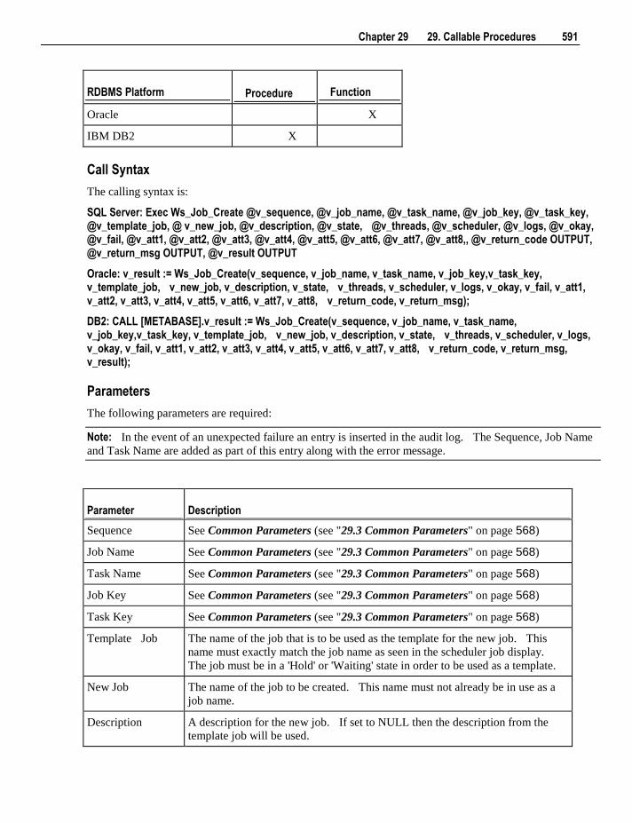
Chapter 29 29. Callable Procedures 591
RDBMS Platform Procedure Function
Oracle X
IBM DB2 X
Call Syntax
The calling syntax is:
SQL Server: Exec Ws_Job_Create @v_sequence, @v_job_name, @v_task_name, @v_job_key, @v_task_key, @v_template_job, @ v_new_job, @v_description, @v_state, @v_threads, @v_scheduler, @v_logs, @v_okay, @v_fail, @v_att1, @v_att2, @v_att3, @v_att4, @v_att5, @v_att6, @v_att7, @v_att8,, @v_return_code OUTPUT, @v_return_msg OUTPUT, @v_result OUTPUT
Oracle: v_result := Ws_Job_Create(v_sequence, v_job_name, v_task_name, v_job_key,v_task_key, v_template_job, v_new_job, v_description, v_state, v_threads, v_scheduler, v_logs, v_okay, v_fail, v_att1, v_att2, v_att3, v_att4, v_att5, v_att6, v_att7, v_att8, v_return_code, v_return_msg);
DB2: CALL [METABASE].v_result := Ws_Job_Create(v_sequence, v_job_name, v_task_name, v_job_key,v_task_key, v_template_job, v_new_job, v_description, v_state, v_threads, v_scheduler, v_logs, v_okay, v_fail, v_att1, v_att2, v_att3, v_att4, v_att5, v_att6, v_att7, v_att8, v_return_code, v_return_msg, v_result);
Parameters
The following parameters are required:
Note: In the event of an unexpected failure an entry is inserted in the audit log. The Sequence, Job Name
and Task Name are added as part of this entry along with the error message.
Parameter Description
Sequence See Common Parameters (see "29.3 Common Parameters" on page 568)
Job Name See Common Parameters (see "29.3 Common Parameters" on page 568)
Task Name See Common Parameters (see "29.3 Common Parameters" on page 568)
Job Key See Common Parameters (see "29.3 Common Parameters" on page 568)
Task Key See Common Parameters (see "29.3 Common Parameters" on page 568)
Template Job The name of the job that is to be used as the template for the new job. This
name must exactly match the job name as seen in the scheduler job display.
The job must be in a 'Hold' or 'Waiting' state in order to be used as a template.
New Job The name of the job to be created. This name must not already be in use as a
job name.
Description A description for the new job. If set to NULL then the description from the
template job will be used.
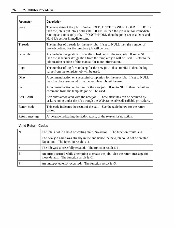
592 29. Callable Procedures
Parameter Description
State The new state of the job. Can be HOLD, ONCE or ONCE+HOLD. If HOLD
then the job is put into a hold state. If ONCE then the job is set for immediate
running as a once only job. If ONCE+HOLD then the job is set as a Once and
Hold job set for immediate start.
Threads The number of threads for the new job. If set to NULL then the number of
threads defined for the template job will be used.
Scheduler A scheduler designation or specific scheduler for the new job. If set to NULL
then the scheduler designation from the template job will be used. Refer to the
job creation section of this manual for more information.
Logs The number of log files to keep for the new job. If set to NULL then the log
value from the template job will be used.
Okay A command action on successful completion for the new job. If set to NULL
then the okay command from the template job will be used.
Fail A command action on failure for the new job. If set to NULL then the failure
command from the template job will be used.
Att1 - Att8 Attributes associated with the new job. These attributes can be acquired by
tasks running under the job through the WsParameterReadJ callable procedure.
Return code This code indicates the result of the call. See the table below for the return
codes.
Return message A message indicating the action taken, or the reason for no action.
Valid Return Codes
N The job is not in a hold or waiting state, No action. The function result is -1.
P The new job name was already in use and hence the new job could not be created.
No action. The function result is -1
S The job was successfully created. The function result is 1.
E An error occurred while attempting to create the job. See the return message for
more details. The function result is -2.
F An unexpected error occurred. The function result is -3.
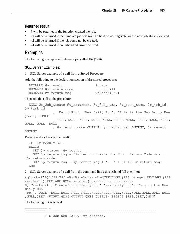
Chapter 29 29. Callable Procedures 593
Returned result
1 will be returned if the function created the job.
–1 will be returned if the template job was not in a hold or waiting state, or the new job already existed.
–2 will be returned if the job could not be created.
–3 will be returned if an unhandled error occurred.
Examples
The following examples all release a job called Daily Run
SQL Server Examples:
1. SQL Server example of a call from a Stored Procedure:
Add the following to the declaration section of the stored procedure:
DECLARE @v_result integer
DECLARE @v_return_code varchar(1)
DECLARE @v_return_msg varchar(256)
Then add the call to the procedure:
EXEC Ws_Job_Create @p_sequence, @p_job_name, @p_task_name, @p_job_id,
@p_task_id
, 'Daily Run', 'New Daily Run', 'This is the New Daily Run
job.', 'ONCE'
, NULL, NULL, NULL, NULL, NULL, NULL, NULL, NULL, NULL, NULL,
NULL, NULL, NULL
, @v_return_code OUTPUT, @v_return_msg OUTPUT, @v_result
OUTPUT
Perhaps add a check of the result:
IF @v_result <> 1
BEGIN
SET @p_status =@v_result
SET @p_return_msg = 'Failed to create the Job. Return Code was '
+@v_return_code
SET @p_return_msg = @p_return_msg + '. ' + RTRIM(@v_return_msg)
END
2. SQL Server example of a call from the command line using sqlcmd (all one line):
sqlcmd -S"SQL SERVER" -WslWarehouse -E -Q"DECLARE @RES integer;DECLARE @RET
varchar(1);DECLARE @MSG varchar(65);EXEC Ws_Job_Create
0,'CreateJob','Create',0,0,'Daily Run','New Daily Run','This is the New
Daily Run
job.','ONCE',NULL,NULL,NULL,NULL,NULL,NULL,NULL,NULL,NULL,NULL,NULL,NULL
,NULL,@RET OUTPUT,@MSG OUTPUT,@RES OUTPUT; SELECT @RES,@RET,@MSG"
The following out is typical:
----------- -
-----------------------------------------------------------------
1 S Job New Daily Run created.
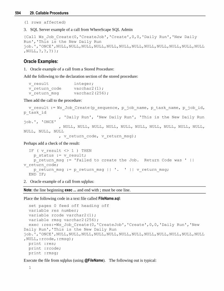
594 29. Callable Procedures
(1 rows affected)
3. SQL Server example of a call from WhereScape SQL Admin
{Call Ws_Job_Create(0,'CreateJob','Create',0,0,'Daily Run','New Daily
Run','This is the New Daily Run
job.','ONCE',NULL,NULL,NULL,NULL,NULL,NULL,NULL,NULL,NULL,NULL,NULL,NULL
,NULL,?,?,?)};
Oracle Examples:
1. Oracle example of a call from a Stored Procedure:
Add the following to the declaration section of the stored procedure:
v_result integer;
v_return_code varchar2(1);
v_return_msg varchar2(256);
Then add the call to the procedure:
v_result := Ws_Job_Create(p_sequence, p_job_name, p_task_name, p_job_id,
p_task_id
, 'Daily Run', 'New Daily Run', 'This is the New Daily Run
job.', 'ONCE'
, NULL, NULL, NULL, NULL, NULL, NULL, NULL, NULL, NULL, NULL,
NULL, NULL, NULL
, v_return_code, v_return_msg);
Perhaps add a check of the result:
IF ( v_result <> 1 ) THEN
p_status := v_result;
p_return_msg := 'Failed to create the Job. Return Code was ' ||
v_return_code;
p_return_msg := p_return_msg || '. ' || v_return_msg;
END IF;
2. Oracle example of a call from sqlplus:
Note: the line beginning exec ... and end with ; must be one line.
Place the following code in a text file called FileName.sql:
set pages 0 feed off heading off
variable res number;
variable rcode varchar2(1);
variable rmsg varchar2(256);
exec :res:=Ws_Job_Create(0,'CreateJob','Create',0,0,'Daily Run','New
Daily Run','This is the New Daily Run
job.','ONCE',NULL,NULL,NULL,NULL,NULL,NULL,NULL,NULL,NULL,NULL,NULL,NULL
,NULL,:rcode,:rmsg);
print :res;
print :rcode;
print :rmsg;
Execute the file from sqlplus (using @FileName). The following out is typical:
1
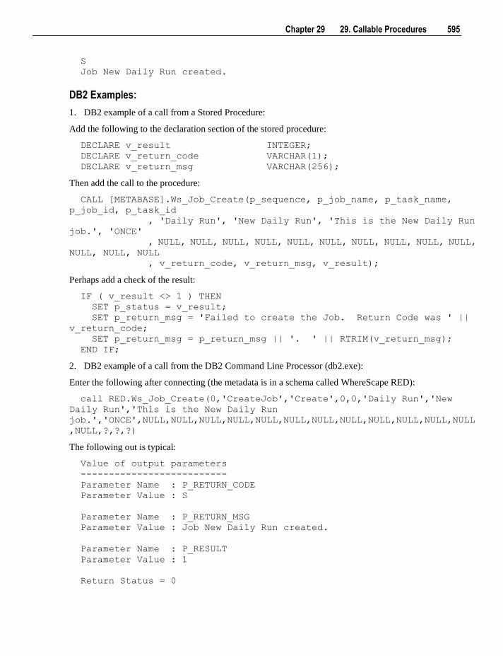
Chapter 29 29. Callable Procedures 595
S
Job New Daily Run created.
DB2 Examples:
1. DB2 example of a call from a Stored Procedure:
Add the following to the declaration section of the stored procedure:
DECLARE v_result INTEGER;
DECLARE v_return_code VARCHAR(1);
DECLARE v_return_msg VARCHAR(256);
Then add the call to the procedure:
CALL [METABASE].Ws_Job_Create(p_sequence, p_job_name, p_task_name,
p_job_id, p_task_id
, 'Daily Run', 'New Daily Run', 'This is the New Daily Run
job.', 'ONCE'
, NULL, NULL, NULL, NULL, NULL, NULL, NULL, NULL, NULL, NULL,
NULL, NULL, NULL
, v_return_code, v_return_msg, v_result);
Perhaps add a check of the result:
IF ( v_result <> 1 ) THEN
SET p_status = v_result;
SET p_return_msg = 'Failed to create the Job. Return Code was ' ||
v_return_code;
SET p_return_msg = p_return_msg || '. ' || RTRIM(v_return_msg);
END IF;
2. DB2 example of a call from the DB2 Command Line Processor (db2.exe):
Enter the following after connecting (the metadata is in a schema called WhereScape RED):
call RED.Ws_Job_Create(0,'CreateJob','Create',0,0,'Daily Run','New
Daily Run','This is the New Daily Run
job.','ONCE',NULL,NULL,NULL,NULL,NULL,NULL,NULL,NULL,NULL,NULL,NULL,NULL
,NULL,?,?,?)
The following out is typical:
Value of output parameters
--------------------------
Parameter Name : P_RETURN_CODE
Parameter Value : S
Parameter Name : P_RETURN_MSG
Parameter Value : Job New Daily Run created.
Parameter Name : P_RESULT
Parameter Value : 1
Return Status = 0
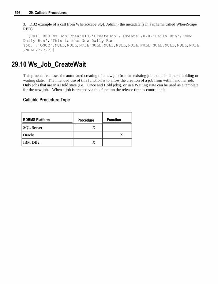
596 29. Callable Procedures
3. DB2 example of a call from WhereScape SQL Admin (the metadata is in a schema called WhereScape
RED):
{Call RED.Ws_Job_Create(0,'CreateJob','Create',0,0,'Daily Run','New
Daily Run','This is the New Daily Run
job.','ONCE',NULL,NULL,NULL,NULL,NULL,NULL,NULL,NULL,NULL,NULL,NULL,NULL
,NULL,?,?,?)}
29.10 Ws_Job_CreateWait
This procedure allows the automated creating of a new job from an existing job that is in either a holding or
waiting state. The intended use of this function is to allow the creation of a job from within another job.
Only jobs that are in a Hold state (i.e. Once and Hold jobs), or in a Waiting state can be used as a template
for the new job. When a job is created via this function the release time is controllable.
Callable Procedure Type
RDBMS Platform Procedure Function
SQL Server X
Oracle X
IBM DB2 X
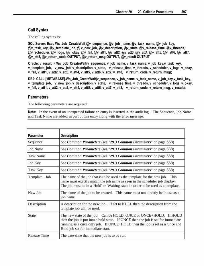
Chapter 29 29. Callable Procedures 597
Call Syntax
The calling syntax is:
SQL Server: Exec Ws_Job_CreateWait @v_sequence, @v_job_name, @v_task_name, @v_job_key, @v_task_key, @v_template_job, @ v_new_job, @v_description, @v_state, @v_release_time, @v_threads, @v_scheduler, @v_logs, @v_okay, @v_fail, @v_att1, @v_att2, @v_att3, @v_att4, @v_att5, @v_att6, @v_att7, @v_att8, @v_return_code OUTPUT, @v_return_msg OUTPUT, @v_result OUTPUT
Oracle: v_result := Ws_Job_CreateWait(v_sequence, v_job_name, v_task_name, v_job_key,v_task_key, v_template_job, v_new_job, v_description, v_state, v_release_time, v_threads, v_scheduler, v_logs, v_okay, v_fail, v_att1, v_att2, v_att3, v_att4, v_att5, v_att6, v_att7, v_att8, v_return_code, v_return_msg);
DB2: CALL [METABASE].Ws_Job_CreateWait(v_sequence, v_job_name, v_task_name, v_job_key,v_task_key, v_template_job, v_new_job, v_description, v_state, v_release_time, v_threads, v_scheduler, v_logs, v_okay, v_fail, v_att1, v_att2, v_att3, v_att4, v_att5, v_att6, v_att7, v_att8, v_return_code, v_return_msg, v_result);
Parameters
The following parameters are required:
Note: In the event of an unexpected failure an entry is inserted in the audit log. The Sequence, Job Name
and Task Name are added as part of this entry along with the error message.
Parameter Description
Sequence See Common Parameters (see "29.3 Common Parameters" on page 568)
Job Name See Common Parameters (see "29.3 Common Parameters" on page 568)
Task Name See Common Parameters (see "29.3 Common Parameters" on page 568)
Job Key See Common Parameters (see "29.3 Common Parameters" on page 568)
Task Key See Common Parameters (see "29.3 Common Parameters" on page 568)
Template Job The name of the job that is to be used as the template for the new job. This
name must exactly match the job name as seen in the scheduler job display.
The job must be in a 'Hold' or 'Waiting' state in order to be used as a template.
New Job The name of the job to be created. This name must not already be in use as a
job name.
Description A description for the new job. If set to NULL then the description from the
template job will be used.
State The new state of the job. Can be HOLD, ONCE or ONCE+HOLD. If HOLD
then the job is put into a hold state. If ONCE then the job is set for immediate
running as a once only job. If ONCE+HOLD then the job is set as a Once and
Hold job set for immediate start.
Release Time The date-time that the new job is to be run.
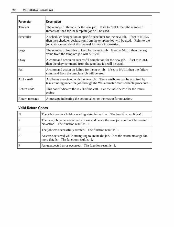
598 29. Callable Procedures
Parameter Description
Threads The number of threads for the new job. If set to NULL then the number of
threads defined for the template job will be used.
Scheduler A scheduler designation or specific scheduler for the new job. If set to NULL
then the scheduler designation from the template job will be used. Refer to the
job creation section of this manual for more information.
Logs The number of log files to keep for the new job. If set to NULL then the log
value from the template job will be used.
Okay A command action on successful completion for the new job. If set to NULL
then the okay command from the template job will be used.
Fail A command action on failure for the new job. If set to NULL then the failure
command from the template job will be used.
Att1 - Att8 Attributes associated with the new job. These attributes can be acquired by
tasks running under the job through the WsParameterReadJ callable procedure.
Return code This code indicates the result of the call. See the table below for the return
codes.
Return message A message indicating the action taken, or the reason for no action.
Valid Return Codes
N The job is not in a hold or waiting state, No action. The function result is -1.
P The new job name was already in use and hence the new job could not be created.
No action. The function result is -1
S The job was successfully created. The function result is 1.
E An error occurred while attempting to create the job. See the return message for
more details. The function result is -2.
F An unexpected error occurred. The function result is -3.
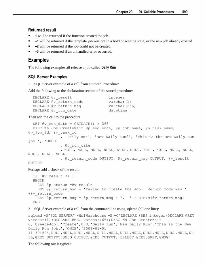
Chapter 29 29. Callable Procedures 599
Returned result
1 will be returned if the function created the job.
–1 will be returned if the template job was not in a hold or waiting state, or the new job already existed.
–2 will be returned if the job could not be created.
–3 will be returned if an unhandled error occurred.
Examples
The following examples all release a job called Daily Run
SQL Server Examples:
1. SQL Server example of a call from a Stored Procedure:
Add the following to the declaration section of the stored procedure:
DECLARE @v_result integer
DECLARE @v_return_code varchar(1)
DECLARE @v_return_msg varchar(256)
DECLARE @v_run_date datetime
Then add the call to the procedure:
SET @v_run_date = GETDATE() + 365
EXEC Ws_Job_CreateWait @p_sequence, @p_job_name, @p_task_name,
@p_job_id, @p_task_id
, 'Daily Run', 'New Daily Run2', 'This is the New Daily Run
job.', 'ONCE'
, @v_run_date
, NULL, NULL, NULL, NULL, NULL, NULL, NULL, NULL, NULL, NULL,
NULL, NULL, NULL
, @v_return_code OUTPUT, @v_return_msg OUTPUT, @v_result
OUTPUT
Perhaps add a check of the result:
IF @v_result <> 1
BEGIN
SET @p_status =@v_result
SET @p_return_msg = 'Failed to create the Job. Return Code was '
+@v_return_code
SET @p_return_msg = @p_return_msg + '. ' + RTRIM(@v_return_msg)
END
2. SQL Server example of a call from the command line using sqlcmd (all one line):
sqlcmd -S"SQL SERVER" -WslWarehouse -E -Q"DECLARE @RES integer;DECLARE @RET
varchar(1);DECLARE @MSG varchar(65);EXEC Ws_Job_CreateWait
0,'CreateJob','Create',0,0,'Daily Run','New Daily Run','This is the New
Daily Run job.','ONCE','2009-01-01
11:30:59',NULL,NULL,NULL,NULL,NULL,NULL,NULL,NULL,NULL,NULL,NULL,NULL,NU
LL,@RET OUTPUT,@MSG OUTPUT,@RES OUTPUT; SELECT @RES,@RET,@MSG"
The following out is typical:
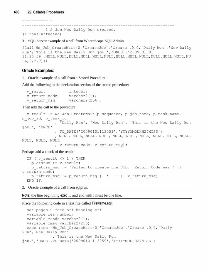
600 29. Callable Procedures
----------- -
-----------------------------------------------------------------
1 S Job New Daily Run created.
(1 rows affected)
3. SQL Server example of a call from WhereScape SQL Admin
{Call Ws_Job_CreateWait(0,'CreateJob','Create',0,0,'Daily Run','New Daily
Run','This is the New Daily Run job.','ONCE','2009-01-01
11:30:59',NULL,NULL,NULL,NULL,NULL,NULL,NULL,NULL,NULL,NULL,NULL,NULL,NU
LL,?,?,?)};
Oracle Examples:
1. Oracle example of a call from a Stored Procedure:
Add the following to the declaration section of the stored procedure:
v_result integer;
v_return_code varchar2(1);
v_return_msg varchar2(256);
Then add the call to the procedure:
v_result := Ws_Job_CreateWait(p_sequence, p_job_name, p_task_name,
p_job_id, p_task_id
, 'Daily Run', 'New Daily Run', 'This is the New Daily Run
job.', 'ONCE'
, TO_DATE('20090101113059','YYYYMMDDHH24MISS')
, NULL, NULL, NULL, NULL, NULL, NULL, NULL, NULL, NULL, NULL,
NULL, NULL, NULL
, v_return_code, v_return_msg);
Perhaps add a check of the result:
IF ( v_result <> 1 ) THEN
p_status := v_result;
p_return_msg := 'Failed to create the Job. Return Code was ' ||
v_return_code;
p_return_msg := p_return_msg || '. ' || v_return_msg;
END IF;
2. Oracle example of a call from sqlplus:
Note: the line beginning exec ... and end with ; must be one line.
Place the following code in a text file called FileName.sql:
set pages 0 feed off heading off
variable res number;
variable rcode varchar2(1);
variable rmsg varchar2(256);
exec :res:=Ws_Job_CreateWait(0,'CreateJob','Create',0,0,'Daily
Run','New Daily Run'
,'This is the New Daily Run
job.','ONCE',TO_DATE('20090101113059','YYYYMMDDHH24MISS')
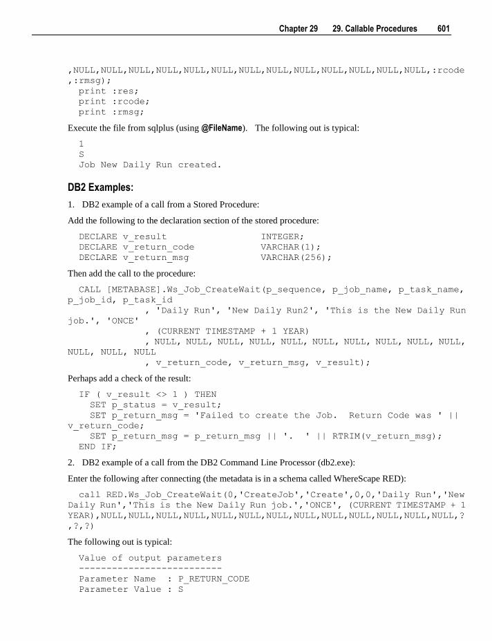
Chapter 29 29. Callable Procedures 601
,NULL,NULL,NULL,NULL,NULL,NULL,NULL,NULL,NULL,NULL,NULL,NULL,NULL,:rcode
,:rmsg);
print :res;
print :rcode;
print :rmsg;
Execute the file from sqlplus (using @FileName). The following out is typical:
1
S
Job New Daily Run created.
DB2 Examples:
1. DB2 example of a call from a Stored Procedure:
Add the following to the declaration section of the stored procedure:
DECLARE v_result INTEGER;
DECLARE v_return_code VARCHAR(1);
DECLARE v_return_msg VARCHAR(256);
Then add the call to the procedure:
CALL [METABASE].Ws_Job_CreateWait(p_sequence, p_job_name, p_task_name,
p_job_id, p_task_id
, 'Daily Run', 'New Daily Run2', 'This is the New Daily Run
job.', 'ONCE'
, (CURRENT TIMESTAMP + 1 YEAR)
, NULL, NULL, NULL, NULL, NULL, NULL, NULL, NULL, NULL, NULL,
NULL, NULL, NULL
, v_return_code, v_return_msg, v_result);
Perhaps add a check of the result:
IF ( v_result <> 1 ) THEN
SET p_status = v_result;
SET p_return_msg = 'Failed to create the Job. Return Code was ' ||
v_return_code;
SET p_return_msg = p_return_msg || '. ' || RTRIM(v_return_msg);
END IF;
2. DB2 example of a call from the DB2 Command Line Processor (db2.exe):
Enter the following after connecting (the metadata is in a schema called WhereScape RED):
call RED.Ws_Job_CreateWait(0,'CreateJob','Create',0,0,'Daily Run','New
Daily Run','This is the New Daily Run job.','ONCE', (CURRENT TIMESTAMP + 1
YEAR),NULL,NULL,NULL,NULL,NULL,NULL,NULL,NULL,NULL,NULL,NULL,NULL,NULL,?
,?,?)
The following out is typical:
Value of output parameters
--------------------------
Parameter Name : P_RETURN_CODE
Parameter Value : S
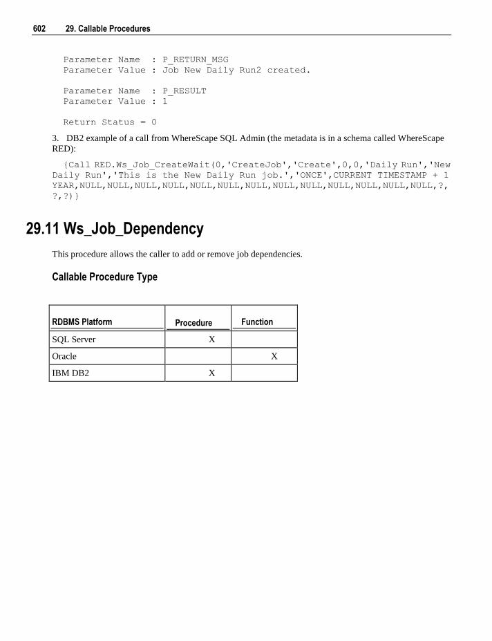
602 29. Callable Procedures
Parameter Name : P_RETURN_MSG
Parameter Value : Job New Daily Run2 created.
Parameter Name : P_RESULT
Parameter Value : 1
Return Status = 0
3. DB2 example of a call from WhereScape SQL Admin (the metadata is in a schema called WhereScape
RED):
{Call RED.Ws_Job_CreateWait(0,'CreateJob','Create',0,0,'Daily Run','New
Daily Run','This is the New Daily Run job.','ONCE',CURRENT TIMESTAMP + 1
YEAR,NULL,NULL,NULL,NULL,NULL,NULL,NULL,NULL,NULL,NULL,NULL,NULL,NULL,?,
?,?)}
29.11 Ws_Job_Dependency
This procedure allows the caller to add or remove job dependencies.
Callable Procedure Type
RDBMS Platform Procedure Function
SQL Server X
Oracle X
IBM DB2 X
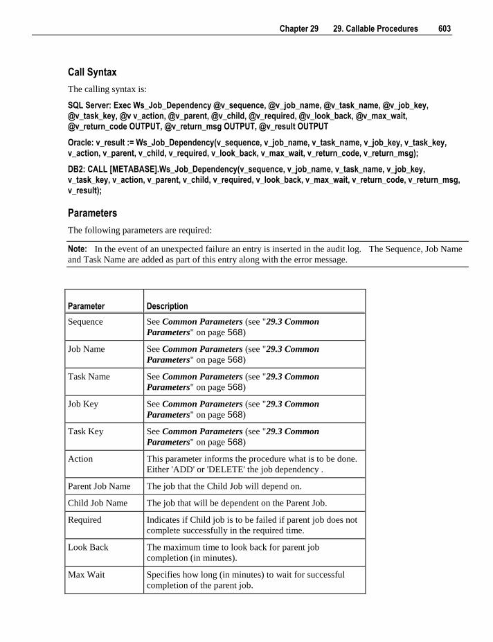
Chapter 29 29. Callable Procedures 603
Call Syntax
The calling syntax is:
SQL Server: Exec Ws_Job_Dependency @v_sequence, @v_job_name, @v_task_name, @v_job_key, @v_task_key, @v v_action, @v_parent, @v_child, @v_required, @v_look_back, @v_max_wait, @v_return_code OUTPUT, @v_return_msg OUTPUT, @v_result OUTPUT
Oracle: v_result := Ws_Job_Dependency(v_sequence, v_job_name, v_task_name, v_job_key, v_task_key, v_action, v_parent, v_child, v_required, v_look_back, v_max_wait, v_return_code, v_return_msg);
DB2: CALL [METABASE].Ws_Job_Dependency(v_sequence, v_job_name, v_task_name, v_job_key, v_task_key, v_action, v_parent, v_child, v_required, v_look_back, v_max_wait, v_return_code, v_return_msg, v_result);
Parameters
The following parameters are required:
Note: In the event of an unexpected failure an entry is inserted in the audit log. The Sequence, Job Name
and Task Name are added as part of this entry along with the error message.
Parameter Description
Sequence See Common Parameters (see "29.3 Common
Parameters" on page 568)
Job Name See Common Parameters (see "29.3 Common
Parameters" on page 568)
Task Name See Common Parameters (see "29.3 Common
Parameters" on page 568)
Job Key See Common Parameters (see "29.3 Common
Parameters" on page 568)
Task Key See Common Parameters (see "29.3 Common
Parameters" on page 568)
Action This parameter informs the procedure what is to be done.
Either 'ADD' or 'DELETE' the job dependency .
Parent Job Name The job that the Child Job will depend on.
Child Job Name The job that will be dependent on the Parent Job.
Required Indicates if Child job is to be failed if parent job does not
complete successfully in the required time.
Look Back The maximum time to look back for parent job
completion (in minutes).
Max Wait Specifies how long (in minutes) to wait for successful
completion of the parent job.
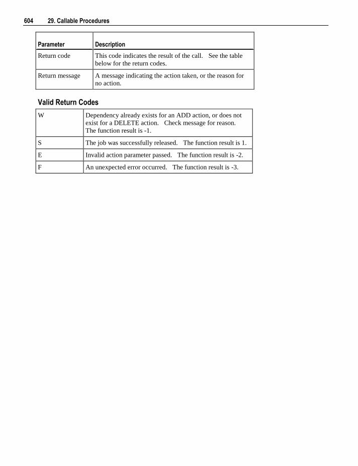
604 29. Callable Procedures
Parameter Description
Return code This code indicates the result of the call. See the table
below for the return codes.
Return message A message indicating the action taken, or the reason for
no action.
Valid Return Codes
W Dependency already exists for an ADD action, or does not
exist for a DELETE action. Check message for reason.
The function result is -1.
S The job was successfully released. The function result is 1.
E Invalid action parameter passed. The function result is -2.
F An unexpected error occurred. The function result is -3.
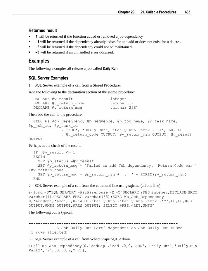
Chapter 29 29. Callable Procedures 605
Returned result
1 will be returned if the function added or removed a job dependency
–1 will be returned if the dependency already exists for and add or does not exist for a delete .
–2 will be returned if the dependency could not be maintained.
–3 will be returned if an unhandled error occurred.
Examples
The following examples all release a job called Daily Run
SQL Server Examples:
1. SQL Server example of a call from a Stored Procedure:
Add the following to the declaration section of the stored procedure:
DECLARE @v_result integer
DECLARE @v_return_code varchar(1)
DECLARE @v_return_msg varchar(256)
Then add the call to the procedure:
EXEC Ws_Job_Dependency @p_sequence, @p_job_name, @p_task_name,
@p_job_id, @p_task_id
, 'ADD', 'Daily Run', 'Daily Run Part2', 'Y', 60, 60
, @v_return_code OUTPUT, @v_return_msg OUTPUT, @v_result
OUTPUT
Perhaps add a check of the result:
IF @v_result <> 1
BEGIN
SET @p_status =@v_result
SET @p_return_msg = 'Failed to add Job dependency. Return Code was '
+@v_return_code
SET @p_return_msg = @p_return_msg + '. ' + RTRIM(@v_return_msg)
END
2. SQL Server example of a call from the command line using sqlcmd (all one line):
sqlcmd -S"SQL SERVER" -WslWarehouse -E -Q"DECLARE @RES integer;DECLARE @RET
varchar(1);DECLARE @MSG varchar(65);EXEC Ws_Job_Dependency
0,'AddDep','Add',0,0,'ADD','Daily Run','Daily Run Part2','Y',60,60,@RET
OUTPUT,@MSG OUTPUT,@RES OUTPUT; SELECT @RES,@RET,@MSG"
The following out is typical:
----------- -
----------------------------------------------------------------
1 S Job Daily Run Part2 dependent on Job Daily Run ADDed
(1 rows affected)
3. SQL Server example of a call from WhereScape SQL Admin
{Call Ws_Job_Dependency(0,'AddDep','Add',0,0,'ADD','Daily Run','Daily Run
Part2','Y',60,60,?,?,?)};
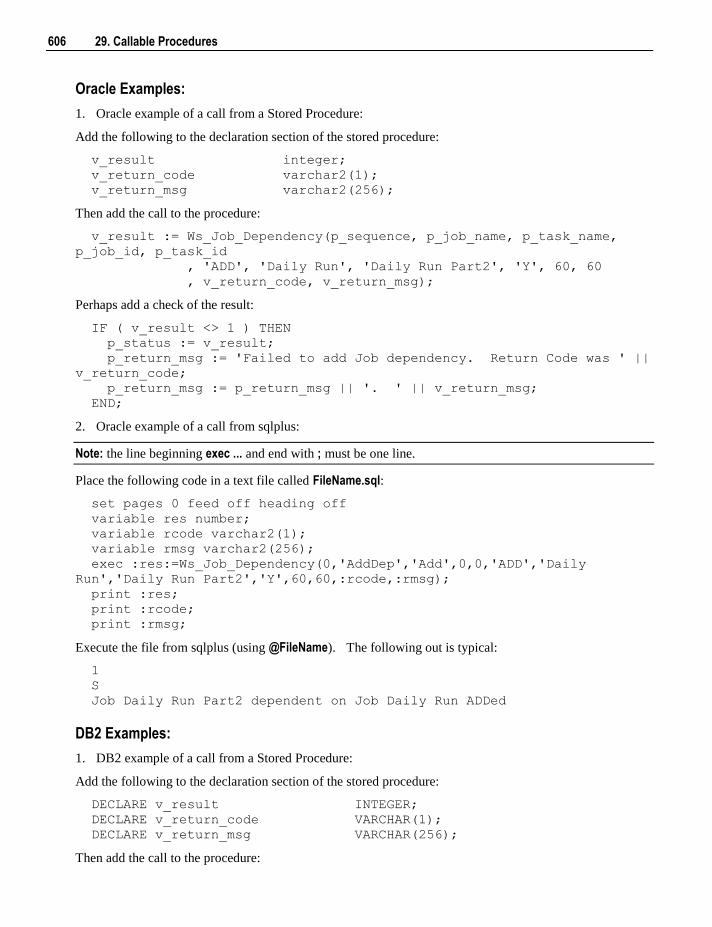
606 29. Callable Procedures
Oracle Examples:
1. Oracle example of a call from a Stored Procedure:
Add the following to the declaration section of the stored procedure:
v_result integer;
v_return_code varchar2(1);
v_return_msg varchar2(256);
Then add the call to the procedure:
v_result := Ws_Job_Dependency(p_sequence, p_job_name, p_task_name,
p_job_id, p_task_id
, 'ADD', 'Daily Run', 'Daily Run Part2', 'Y', 60, 60
, v_return_code, v_return_msg);
Perhaps add a check of the result:
IF ( v_result <> 1 ) THEN
p_status := v_result;
p_return_msg := 'Failed to add Job dependency. Return Code was ' ||
v_return_code;
p_return_msg := p_return_msg || '. ' || v_return_msg;
END;
2. Oracle example of a call from sqlplus:
Note: the line beginning exec ... and end with ; must be one line.
Place the following code in a text file called FileName.sql:
set pages 0 feed off heading off
variable res number;
variable rcode varchar2(1);
variable rmsg varchar2(256);
exec :res:=Ws_Job_Dependency(0,'AddDep','Add',0,0,'ADD','Daily
Run','Daily Run Part2','Y',60,60,:rcode,:rmsg);
print :res;
print :rcode;
print :rmsg;
Execute the file from sqlplus (using @FileName). The following out is typical:
1
S
Job Daily Run Part2 dependent on Job Daily Run ADDed
DB2 Examples:
1. DB2 example of a call from a Stored Procedure:
Add the following to the declaration section of the stored procedure:
DECLARE v_result INTEGER;
DECLARE v_return_code VARCHAR(1);
DECLARE v_return_msg VARCHAR(256);
Then add the call to the procedure:
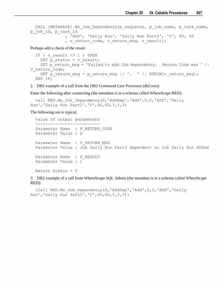
Chapter 29 29. Callable Procedures 607
CALL [METABASE].Ws_Job_Dependency(p_sequence, p_job_name, p_task_name,
p_job_id, p_task_id
, 'ADD', 'Daily Run', 'Daily Run Part2', 'Y', 60, 60
, v_return_code, v_return_msg, v_result);
Perhaps add a check of the result:
IF ( v_result <> 1 ) THEN
SET p_status = v_result;
SET p_return_msg = 'Failed to add Job dependency. Return Code was ' ||
v_return_code;
SET p_return_msg = p_return_msg || '. ' || RTRIM(v_return_msg);
END IF;
2. DB2 example of a call from the DB2 Command Line Processor (db2.exe):
Enter the following after connecting (the metadata is in a schema called WhereScape RED):
call RED.Ws_Job_Dependency(0,'AddDep','Add',0,0,'ADD','Daily
Run','Daily Run Part2','Y',60,60,?,?,?)
The following out is typical:
Value of output parameters
--------------------------
Parameter Name : P_RETURN_CODE
Parameter Value : S
Parameter Name : P_RETURN_MSG
Parameter Value : Job Daily Run Part2 dependent on Job Daily Run ADDed
Parameter Name : P_RESULT
Parameter Value : 1
Return Status = 0
3. DB2 example of a call from WhereScape SQL Admin (the metadata is in a schema called WhereScape
RED):
{Call RED.Ws_Job_Dependency(0,'AddDep','Add',0,0,'ADD','Daily
Run','Daily Run Part2','Y',60,60,?,?,?)}
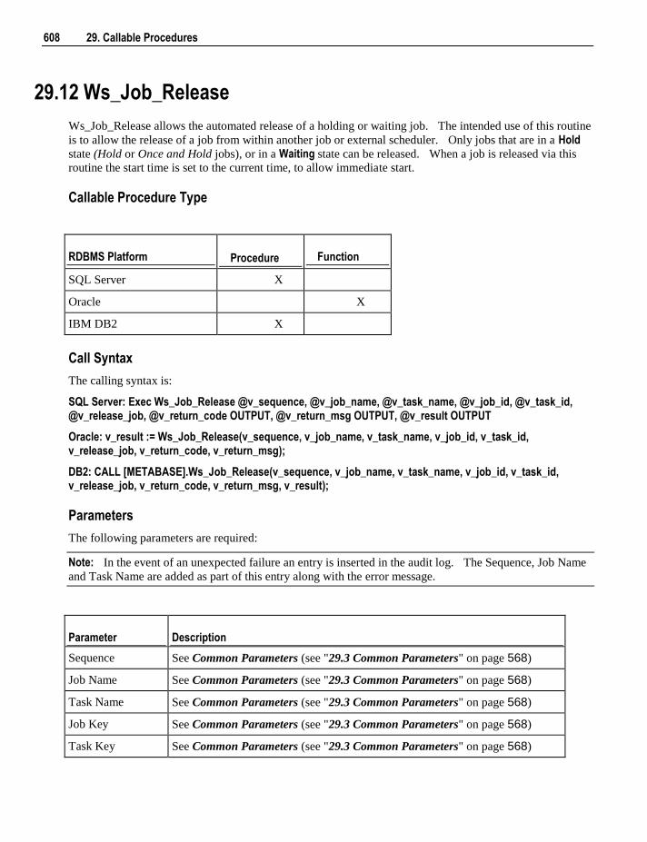
608 29. Callable Procedures
29.12 Ws_Job_Release
Ws_Job_Release allows the automated release of a holding or waiting job. The intended use of this routine
is to allow the release of a job from within another job or external scheduler. Only jobs that are in a Hold state (Hold or Once and Hold jobs), or in a Waiting state can be released. When a job is released via this
routine the start time is set to the current time, to allow immediate start.
Callable Procedure Type
RDBMS Platform Procedure Function
SQL Server X
Oracle X
IBM DB2 X
Call Syntax
The calling syntax is:
SQL Server: Exec Ws_Job_Release @v_sequence, @v_job_name, @v_task_name, @v_job_id, @v_task_id, @v_release_job, @v_return_code OUTPUT, @v_return_msg OUTPUT, @v_result OUTPUT
Oracle: v_result := Ws_Job_Release(v_sequence, v_job_name, v_task_name, v_job_id, v_task_id, v_release_job, v_return_code, v_return_msg);
DB2: CALL [METABASE].Ws_Job_Release(v_sequence, v_job_name, v_task_name, v_job_id, v_task_id, v_release_job, v_return_code, v_return_msg, v_result);
Parameters
The following parameters are required:
Note: In the event of an unexpected failure an entry is inserted in the audit log. The Sequence, Job Name
and Task Name are added as part of this entry along with the error message.
Parameter Description
Sequence See Common Parameters (see "29.3 Common Parameters" on page 568)
Job Name See Common Parameters (see "29.3 Common Parameters" on page 568)
Task Name See Common Parameters (see "29.3 Common Parameters" on page 568)
Job Key See Common Parameters (see "29.3 Common Parameters" on page 568)
Task Key See Common Parameters (see "29.3 Common Parameters" on page 568)
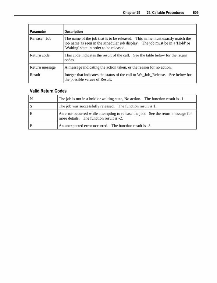
Chapter 29 29. Callable Procedures 609
Parameter Description
Release Job The name of the job that is to be released. This name must exactly match the
job name as seen in the scheduler job display. The job must be in a 'Hold' or
'Waiting' state in order to be released.
Return code This code indicates the result of the call. See the table below for the return
codes.
Return message A message indicating the action taken, or the reason for no action.
Result Integer that indicates the status of the call to Ws_Job_Release. See below for
the possible values of Result.
Valid Return Codes
N The job is not in a hold or waiting state, No action. The function result is -1.
S The job was successfully released. The function result is 1.
E An error occurred while attempting to release the job. See the return message for
more details. The function result is -2.
F An unexpected error occurred. The function result is -3.
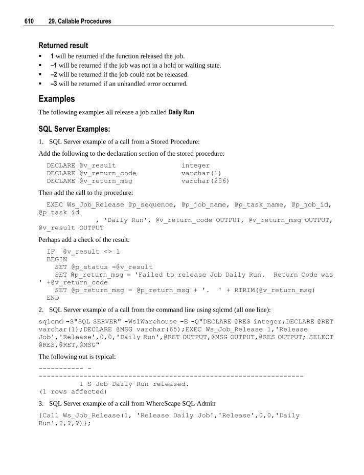
610 29. Callable Procedures
Returned result
1 will be returned if the function released the job.
–1 will be returned if the job was not in a hold or waiting state.
–2 will be returned if the job could not be released.
–3 will be returned if an unhandled error occurred.
Examples
The following examples all release a job called Daily Run
SQL Server Examples:
1. SQL Server example of a call from a Stored Procedure:
Add the following to the declaration section of the stored procedure:
DECLARE @v_result integer
DECLARE @v_return_code varchar(1)
DECLARE @v_return_msg varchar(256)
Then add the call to the procedure:
EXEC Ws_Job_Release @p_sequence, @p_job_name, @p_task_name, @p_job_id,
@p_task_id
, 'Daily Run', @v_return_code OUTPUT, @v_return_msg OUTPUT,
@v_result OUTPUT
Perhaps add a check of the result:
IF @v_result <> 1
BEGIN
SET @p_status =@v_result
SET @p_return_msg = 'Failed to release Job Daily Run. Return Code was
' +@v_return_code
SET @p_return_msg = @p_return_msg + '. ' + RTRIM(@v_return_msg)
END
2. SQL Server example of a call from the command line using sqlcmd (all one line):
sqlcmd -S"SQL SERVER" -WslWarehouse -E -Q"DECLARE @RES integer;DECLARE @RET
varchar(1);DECLARE @MSG varchar(65);EXEC Ws_Job_Release 1,'Release
Job','Release',0,0,'Daily Run',@RET OUTPUT,@MSG OUTPUT,@RES OUTPUT; SELECT
@RES,@RET,@MSG"
The following out is typical:
----------- -
-----------------------------------------------------------------
1 S Job Daily Run released.
(1 rows affected)
3. SQL Server example of a call from WhereScape SQL Admin
{Call Ws_Job_Release(1, 'Release Daily Job','Release',0,0,'Daily
Run',?,?,?)};
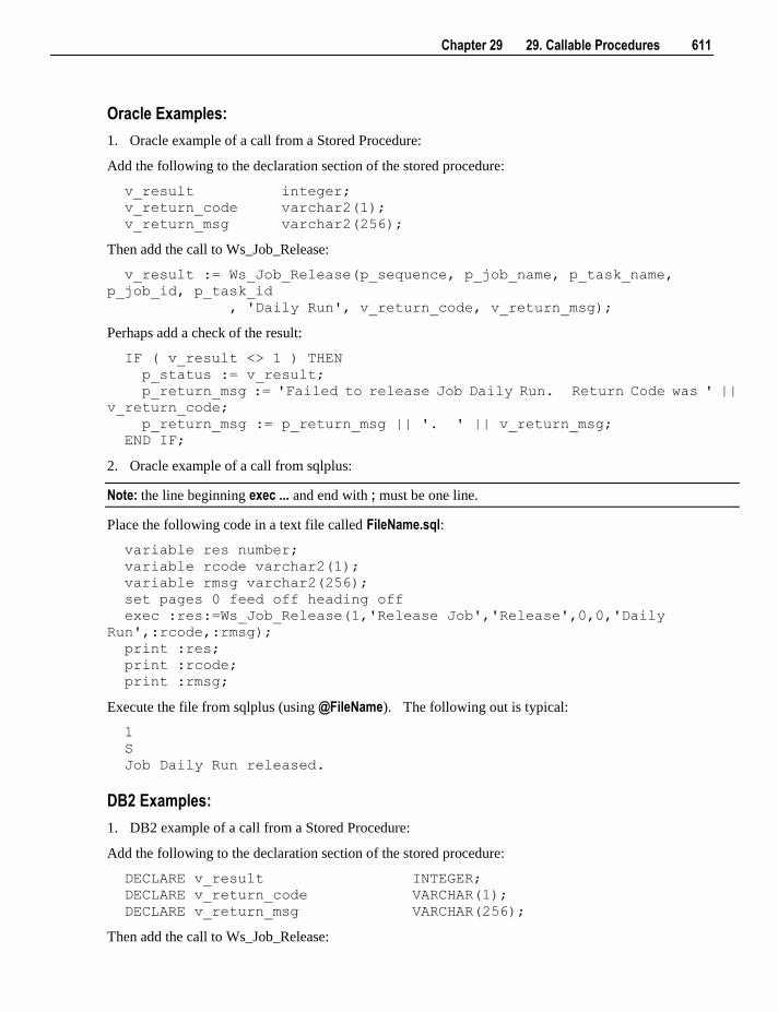
Chapter 29 29. Callable Procedures 611
Oracle Examples:
1. Oracle example of a call from a Stored Procedure:
Add the following to the declaration section of the stored procedure:
v_result integer;
v_return_code varchar2(1);
v_return_msg varchar2(256);
Then add the call to Ws_Job_Release:
v_result := Ws_Job_Release(p_sequence, p_job_name, p_task_name,
p_job_id, p_task_id
, 'Daily Run', v_return_code, v_return_msg);
Perhaps add a check of the result:
IF ( v_result <> 1 ) THEN
p_status := v_result;
p_return_msg := 'Failed to release Job Daily Run. Return Code was ' ||
v_return_code;
p_return_msg := p_return_msg || '. ' || v_return_msg;
END IF;
2. Oracle example of a call from sqlplus:
Note: the line beginning exec ... and end with ; must be one line.
Place the following code in a text file called FileName.sql:
variable res number;
variable rcode varchar2(1);
variable rmsg varchar2(256);
set pages 0 feed off heading off
exec :res:=Ws_Job_Release(1,'Release Job','Release',0,0,'Daily
Run',:rcode,:rmsg);
print :res;
print :rcode;
print :rmsg;
Execute the file from sqlplus (using @FileName). The following out is typical:
1
S
Job Daily Run released.
DB2 Examples:
1. DB2 example of a call from a Stored Procedure:
Add the following to the declaration section of the stored procedure:
DECLARE v_result INTEGER;
DECLARE v_return_code VARCHAR(1);
DECLARE v_return_msg VARCHAR(256);
Then add the call to Ws_Job_Release:
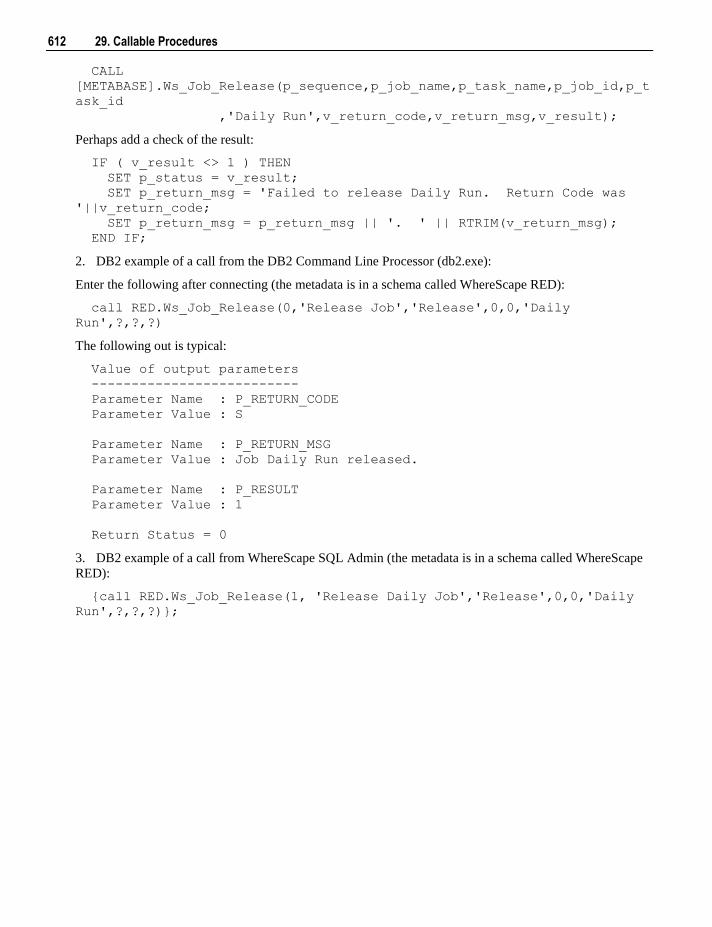
612 29. Callable Procedures
CALL
[METABASE].Ws_Job_Release(p_sequence,p_job_name,p_task_name,p_job_id,p_t
ask_id
,'Daily Run',v_return_code,v_return_msg,v_result);
Perhaps add a check of the result:
IF ( v_result <> 1 ) THEN
SET p_status = v_result;
SET p_return_msg = 'Failed to release Daily Run. Return Code was
'||v_return_code;
SET p_return_msg = p_return_msg || '. ' || RTRIM(v_return_msg);
END IF;
2. DB2 example of a call from the DB2 Command Line Processor (db2.exe):
Enter the following after connecting (the metadata is in a schema called WhereScape RED):
call RED.Ws_Job_Release(0,'Release Job','Release',0,0,'Daily
Run',?,?,?)
The following out is typical:
Value of output parameters
--------------------------
Parameter Name : P_RETURN_CODE
Parameter Value : S
Parameter Name : P_RETURN_MSG
Parameter Value : Job Daily Run released.
Parameter Name : P_RESULT
Parameter Value : 1
Return Status = 0
3. DB2 example of a call from WhereScape SQL Admin (the metadata is in a schema called WhereScape
RED):
{call RED.Ws_Job_Release(1, 'Release Daily Job','Release',0,0,'Daily
Run',?,?,?)};
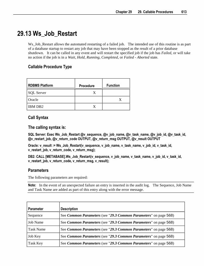
Chapter 29 29. Callable Procedures 613
29.13 Ws_Job_Restart
Ws_Job_Restart allows the automated restarting of a failed job. The intended use of this routine is as part
of a database startup to restart any job that may have been stopped as the result of a prior database
shutdown. It can be called in any event and will restart the specified job if the job has Failed, or will take
no action if the job is in a Wait, Hold, Running, Completed, or Failed - Aborted state.
Callable Procedure Type
RDBMS Platform Procedure Function
SQL Server X
Oracle X
IBM DB2 X
Call Syntax
The calling syntax is:
SQL Server: Exec Ws_Job_Restart @v_sequence, @v_job_name, @v_task_name, @v_job_id, @v_task_id, @v_restart_job, @v_return_code OUTPUT, @v_return_msg OUTPUT, @v_result OUTPUT
Oracle: v_result := Ws_Job_Restart(v_sequence, v_job_name, v_task_name, v_job_id, v_task_id, v_restart_job, v_return_code, v_return_msg);
DB2: CALL [METABASE].Ws_Job_Restart(v_sequence, v_job_name, v_task_name, v_job_id, v_task_id, v_restart_job, v_return_code, v_return_msg, v_result);
Parameters
The following parameters are required:
Note: In the event of an unexpected failure an entry is inserted in the audit log. The Sequence, Job Name
and Task Name are added as part of this entry along with the error message.
Parameter Description
Sequence See Common Parameters (see "29.3 Common Parameters" on page 568)
Job Name See Common Parameters (see "29.3 Common Parameters" on page 568)
Task Name See Common Parameters (see "29.3 Common Parameters" on page 568)
Job Key See Common Parameters (see "29.3 Common Parameters" on page 568)
Task Key See Common Parameters (see "29.3 Common Parameters" on page 568)
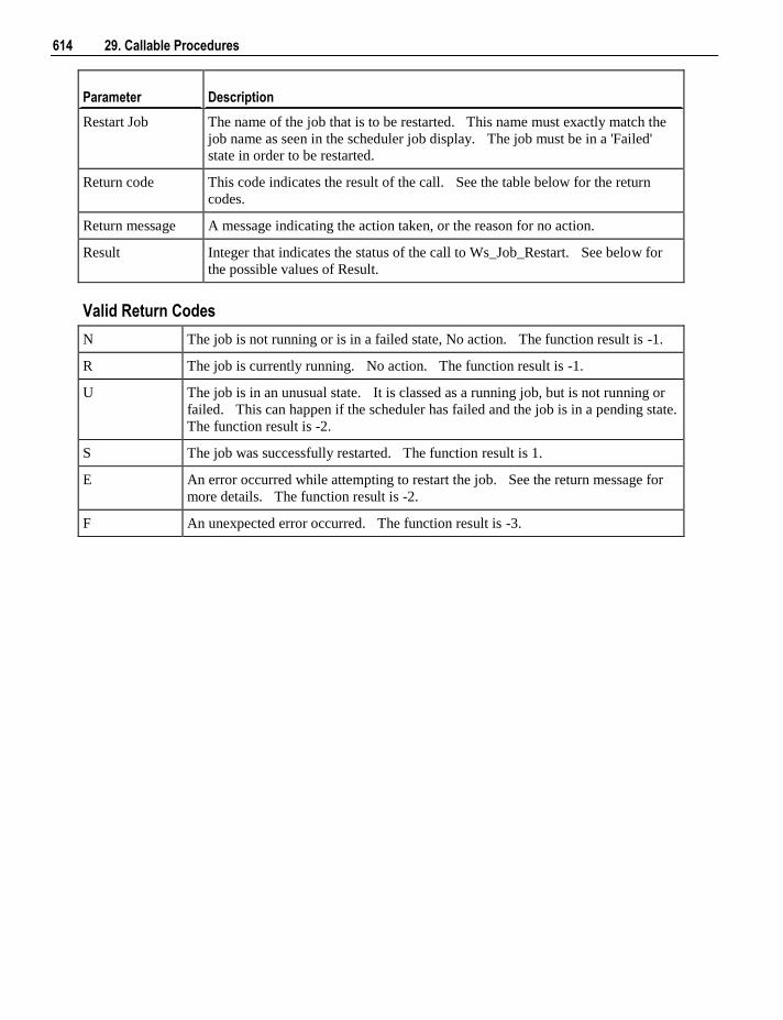
614 29. Callable Procedures
Parameter Description
Restart Job The name of the job that is to be restarted. This name must exactly match the
job name as seen in the scheduler job display. The job must be in a 'Failed'
state in order to be restarted.
Return code This code indicates the result of the call. See the table below for the return
codes.
Return message A message indicating the action taken, or the reason for no action.
Result Integer that indicates the status of the call to Ws_Job_Restart. See below for
the possible values of Result.
Valid Return Codes
N The job is not running or is in a failed state, No action. The function result is -1.
R The job is currently running. No action. The function result is -1.
U The job is in an unusual state. It is classed as a running job, but is not running or
failed. This can happen if the scheduler has failed and the job is in a pending state.
The function result is -2.
S The job was successfully restarted. The function result is 1.
E An error occurred while attempting to restart the job. See the return message for
more details. The function result is -2.
F An unexpected error occurred. The function result is -3.
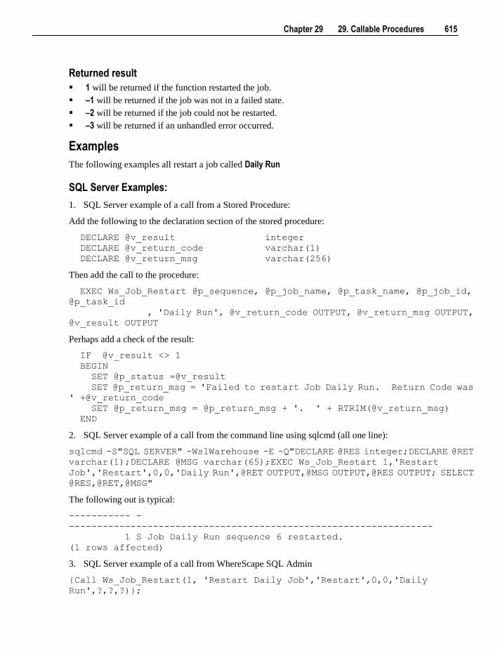
Chapter 29 29. Callable Procedures 615
Returned result
1 will be returned if the function restarted the job.
–1 will be returned if the job was not in a failed state.
–2 will be returned if the job could not be restarted.
–3 will be returned if an unhandled error occurred.
Examples
The following examples all restart a job called Daily Run
SQL Server Examples:
1. SQL Server example of a call from a Stored Procedure:
Add the following to the declaration section of the stored procedure:
DECLARE @v_result integer
DECLARE @v_return_code varchar(1)
DECLARE @v_return_msg varchar(256)
Then add the call to the procedure:
EXEC Ws_Job_Restart @p_sequence, @p_job_name, @p_task_name, @p_job_id,
@p_task_id
, 'Daily Run', @v_return_code OUTPUT, @v_return_msg OUTPUT,
@v_result OUTPUT
Perhaps add a check of the result:
IF @v_result <> 1
BEGIN
SET @p_status =@v_result
SET @p_return_msg = 'Failed to restart Job Daily Run. Return Code was
' +@v_return_code
SET @p_return_msg = @p_return_msg + '. ' + RTRIM(@v_return_msg)
END
2. SQL Server example of a call from the command line using sqlcmd (all one line):
sqlcmd -S"SQL SERVER" -WslWarehouse -E -Q"DECLARE @RES integer;DECLARE @RET
varchar(1);DECLARE @MSG varchar(65);EXEC Ws_Job_Restart 1,'Restart
Job','Restart',0,0,'Daily Run',@RET OUTPUT,@MSG OUTPUT,@RES OUTPUT; SELECT
@RES,@RET,@MSG"
The following out is typical:
----------- -
-----------------------------------------------------------------
1 S Job Daily Run sequence 6 restarted.
(1 rows affected)
3. SQL Server example of a call from WhereScape SQL Admin
{Call Ws_Job_Restart(1, 'Restart Daily Job','Restart',0,0,'Daily
Run',?,?,?)};
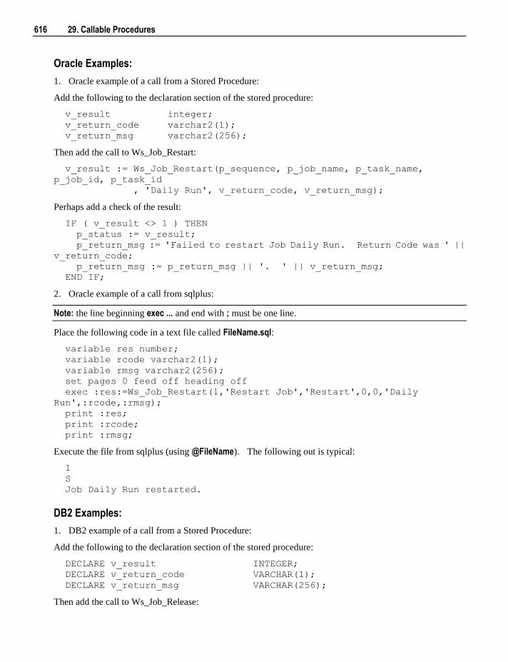
616 29. Callable Procedures
Oracle Examples:
1. Oracle example of a call from a Stored Procedure:
Add the following to the declaration section of the stored procedure:
v_result integer;
v_return_code varchar2(1);
v_return_msg varchar2(256);
Then add the call to Ws_Job_Restart:
v_result := Ws_Job_Restart(p_sequence, p_job_name, p_task_name,
p_job_id, p_task_id
, 'Daily Run', v_return_code, v_return_msg);
Perhaps add a check of the result:
IF ( v_result <> 1 ) THEN
p_status := v_result;
p_return_msg := 'Failed to restart Job Daily Run. Return Code was ' ||
v_return_code;
p_return_msg := p_return_msg || '. ' || v_return_msg;
END IF;
2. Oracle example of a call from sqlplus:
Note: the line beginning exec ... and end with ; must be one line.
Place the following code in a text file called FileName.sql:
variable res number;
variable rcode varchar2(1);
variable rmsg varchar2(256);
set pages 0 feed off heading off
exec :res:=Ws_Job_Restart(1,'Restart Job','Restart',0,0,'Daily
Run',:rcode,:rmsg);
print :res;
print :rcode;
print :rmsg;
Execute the file from sqlplus (using @FileName). The following out is typical:
1
S
Job Daily Run restarted.
DB2 Examples:
1. DB2 example of a call from a Stored Procedure:
Add the following to the declaration section of the stored procedure:
DECLARE v_result INTEGER;
DECLARE v_return_code VARCHAR(1);
DECLARE v_return_msg VARCHAR(256);
Then add the call to Ws_Job_Release:
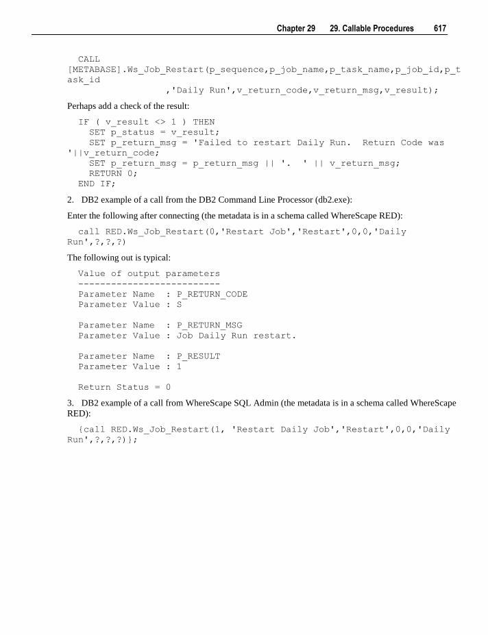
Chapter 29 29. Callable Procedures 617
CALL
[METABASE].Ws_Job_Restart(p_sequence,p_job_name,p_task_name,p_job_id,p_t
ask_id
,'Daily Run',v_return_code,v_return_msg,v_result);
Perhaps add a check of the result:
IF ( v_result <> 1 ) THEN
SET p_status = v_result;
SET p_return_msg = 'Failed to restart Daily Run. Return Code was
'||v_return_code;
SET p_return_msg = p_return_msg || '. ' || v_return_msg;
RETURN 0;
END IF;
2. DB2 example of a call from the DB2 Command Line Processor (db2.exe):
Enter the following after connecting (the metadata is in a schema called WhereScape RED):
call RED.Ws_Job_Restart(0,'Restart Job','Restart',0,0,'Daily
Run',?,?,?)
The following out is typical:
Value of output parameters
--------------------------
Parameter Name : P_RETURN_CODE
Parameter Value : S
Parameter Name : P_RETURN_MSG
Parameter Value : Job Daily Run restart.
Parameter Name : P_RESULT
Parameter Value : 1
Return Status = 0
3. DB2 example of a call from WhereScape SQL Admin (the metadata is in a schema called WhereScape
RED):
{call RED.Ws_Job_Restart(1, 'Restart Daily Job','Restart',0,0,'Daily
Run',?,?,?)};
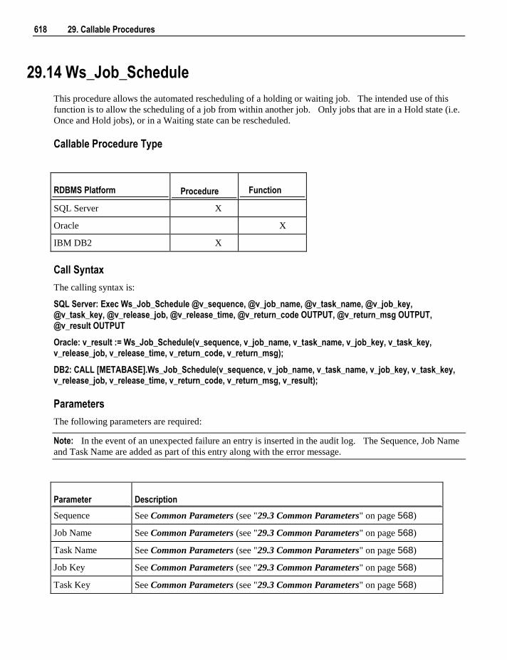
618 29. Callable Procedures
29.14 Ws_Job_Schedule
This procedure allows the automated rescheduling of a holding or waiting job. The intended use of this
function is to allow the scheduling of a job from within another job. Only jobs that are in a Hold state (i.e.
Once and Hold jobs), or in a Waiting state can be rescheduled.
Callable Procedure Type
RDBMS Platform Procedure Function
SQL Server X
Oracle X
IBM DB2 X
Call Syntax
The calling syntax is:
SQL Server: Exec Ws_Job_Schedule @v_sequence, @v_job_name, @v_task_name, @v_job_key, @v_task_key, @v_release_job, @v_release_time, @v_return_code OUTPUT, @v_return_msg OUTPUT, @v_result OUTPUT
Oracle: v_result := Ws_Job_Schedule(v_sequence, v_job_name, v_task_name, v_job_key, v_task_key, v_release_job, v_release_time, v_return_code, v_return_msg);
DB2: CALL [METABASE].Ws_Job_Schedule(v_sequence, v_job_name, v_task_name, v_job_key, v_task_key, v_release_job, v_release_time, v_return_code, v_return_msg, v_result);
Parameters
The following parameters are required:
Note: In the event of an unexpected failure an entry is inserted in the audit log. The Sequence, Job Name
and Task Name are added as part of this entry along with the error message.
Parameter Description
Sequence See Common Parameters (see "29.3 Common Parameters" on page 568)
Job Name See Common Parameters (see "29.3 Common Parameters" on page 568)
Task Name See Common Parameters (see "29.3 Common Parameters" on page 568)
Job Key See Common Parameters (see "29.3 Common Parameters" on page 568)
Task Key See Common Parameters (see "29.3 Common Parameters" on page 568)
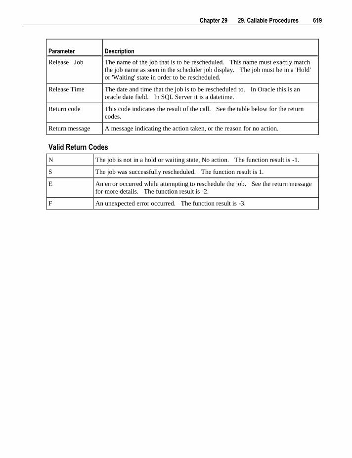
Chapter 29 29. Callable Procedures 619
Parameter Description
Release Job The name of the job that is to be rescheduled. This name must exactly match
the job name as seen in the scheduler job display. The job must be in a 'Hold'
or 'Waiting' state in order to be rescheduled.
Release Time The date and time that the job is to be rescheduled to. In Oracle this is an
oracle date field. In SQL Server it is a datetime.
Return code This code indicates the result of the call. See the table below for the return
codes.
Return message A message indicating the action taken, or the reason for no action.
Valid Return Codes
N The job is not in a hold or waiting state, No action. The function result is -1.
S The job was successfully rescheduled. The function result is 1.
E An error occurred while attempting to reschedule the job. See the return message
for more details. The function result is -2.
F An unexpected error occurred. The function result is -3.
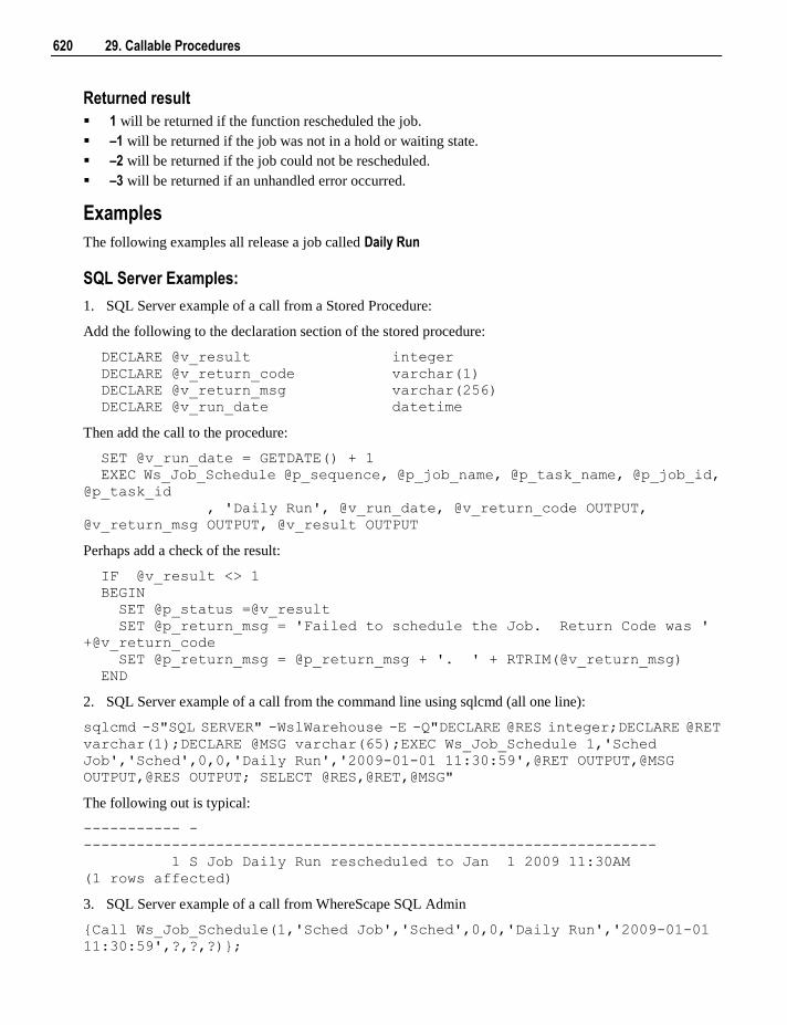
620 29. Callable Procedures
Returned result
1 will be returned if the function rescheduled the job.
–1 will be returned if the job was not in a hold or waiting state.
–2 will be returned if the job could not be rescheduled.
–3 will be returned if an unhandled error occurred.
Examples
The following examples all release a job called Daily Run
SQL Server Examples:
1. SQL Server example of a call from a Stored Procedure:
Add the following to the declaration section of the stored procedure:
DECLARE @v_result integer
DECLARE @v_return_code varchar(1)
DECLARE @v_return_msg varchar(256)
DECLARE @v_run_date datetime
Then add the call to the procedure:
SET @v_run_date = GETDATE() + 1
EXEC Ws_Job_Schedule @p_sequence, @p_job_name, @p_task_name, @p_job_id,
@p_task_id
, 'Daily Run', @v_run_date, @v_return_code OUTPUT,
@v_return_msg OUTPUT, @v_result OUTPUT
Perhaps add a check of the result:
IF @v_result <> 1
BEGIN
SET @p_status =@v_result
SET @p_return_msg = 'Failed to schedule the Job. Return Code was '
+@v_return_code
SET @p_return_msg = @p_return_msg + '. ' + RTRIM(@v_return_msg)
END
2. SQL Server example of a call from the command line using sqlcmd (all one line):
sqlcmd -S"SQL SERVER" -WslWarehouse -E -Q"DECLARE @RES integer;DECLARE @RET
varchar(1);DECLARE @MSG varchar(65);EXEC Ws_Job_Schedule 1,'Sched
Job','Sched',0,0,'Daily Run','2009-01-01 11:30:59',@RET OUTPUT,@MSG
OUTPUT,@RES OUTPUT; SELECT @RES,@RET,@MSG"
The following out is typical:
----------- -
-----------------------------------------------------------------
1 S Job Daily Run rescheduled to Jan 1 2009 11:30AM
(1 rows affected)
3. SQL Server example of a call from WhereScape SQL Admin
{Call Ws_Job_Schedule(1,'Sched Job','Sched',0,0,'Daily Run','2009-01-01
11:30:59',?,?,?)};
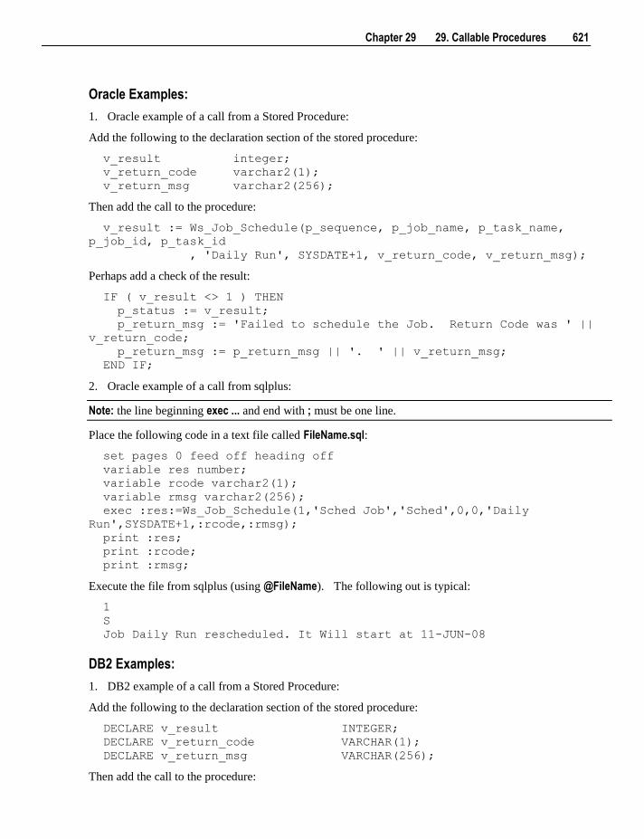
Chapter 29 29. Callable Procedures 621
Oracle Examples:
1. Oracle example of a call from a Stored Procedure:
Add the following to the declaration section of the stored procedure:
v_result integer;
v_return_code varchar2(1);
v_return_msg varchar2(256);
Then add the call to the procedure:
v_result := Ws_Job_Schedule(p_sequence, p_job_name, p_task_name,
p_job_id, p_task_id
, 'Daily Run', SYSDATE+1, v_return_code, v_return_msg);
Perhaps add a check of the result:
IF ( v_result <> 1 ) THEN
p_status := v_result;
p_return_msg := 'Failed to schedule the Job. Return Code was ' ||
v_return_code;
p_return_msg := p_return_msg || '. ' || v_return_msg;
END IF;
2. Oracle example of a call from sqlplus:
Note: the line beginning exec ... and end with ; must be one line.
Place the following code in a text file called FileName.sql:
set pages 0 feed off heading off
variable res number;
variable rcode varchar2(1);
variable rmsg varchar2(256);
exec :res:=Ws_Job_Schedule(1,'Sched Job','Sched',0,0,'Daily
Run',SYSDATE+1,:rcode,:rmsg);
print :res;
print :rcode;
print :rmsg;
Execute the file from sqlplus (using @FileName). The following out is typical:
1
S
Job Daily Run rescheduled. It Will start at 11-JUN-08
DB2 Examples:
1. DB2 example of a call from a Stored Procedure:
Add the following to the declaration section of the stored procedure:
DECLARE v_result INTEGER;
DECLARE v_return_code VARCHAR(1);
DECLARE v_return_msg VARCHAR(256);
Then add the call to the procedure:
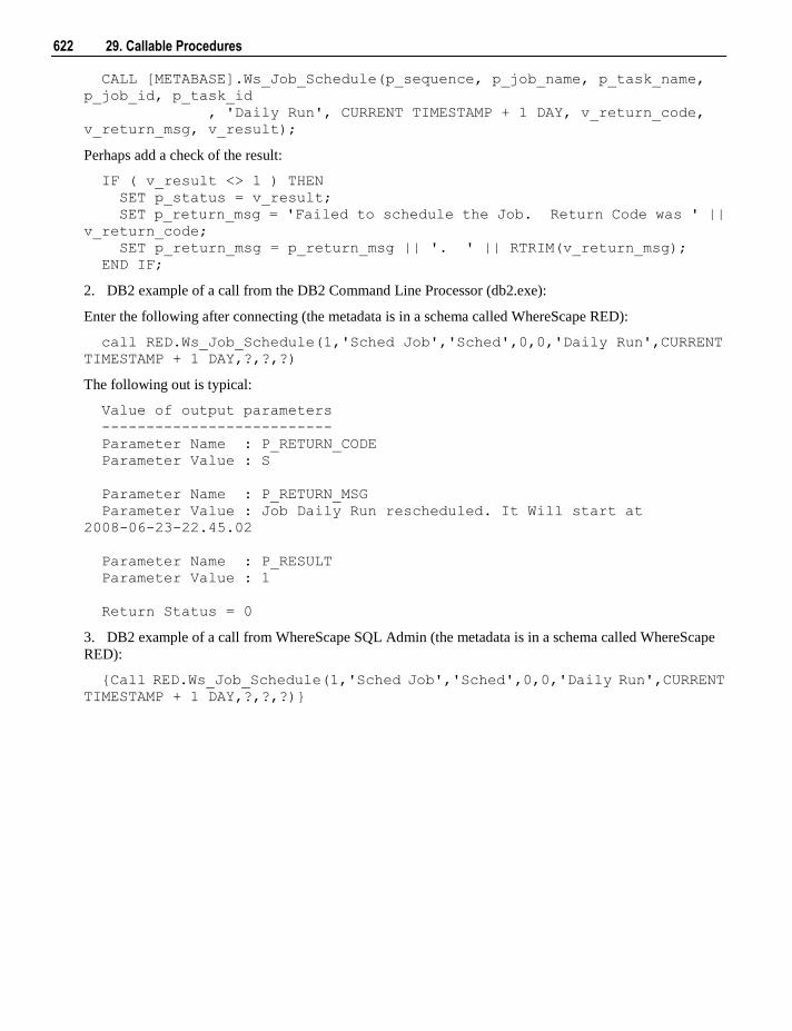
622 29. Callable Procedures
CALL [METABASE].Ws_Job_Schedule(p_sequence, p_job_name, p_task_name,
p_job_id, p_task_id
, 'Daily Run', CURRENT TIMESTAMP + 1 DAY, v_return_code,
v_return_msg, v_result);
Perhaps add a check of the result:
IF ( v_result <> 1 ) THEN
SET p_status = v_result;
SET p_return_msg = 'Failed to schedule the Job. Return Code was ' ||
v_return_code;
SET p_return_msg = p_return_msg || '. ' || RTRIM(v_return_msg);
END IF;
2. DB2 example of a call from the DB2 Command Line Processor (db2.exe):
Enter the following after connecting (the metadata is in a schema called WhereScape RED):
call RED.Ws_Job_Schedule(1,'Sched Job','Sched',0,0,'Daily Run',CURRENT
TIMESTAMP + 1 DAY,?,?,?)
The following out is typical:
Value of output parameters
--------------------------
Parameter Name : P_RETURN_CODE
Parameter Value : S
Parameter Name : P_RETURN_MSG
Parameter Value : Job Daily Run rescheduled. It Will start at
2008-06-23-22.45.02
Parameter Name : P_RESULT
Parameter Value : 1
Return Status = 0
3. DB2 example of a call from WhereScape SQL Admin (the metadata is in a schema called WhereScape
RED):
{Call RED.Ws_Job_Schedule(1,'Sched Job','Sched',0,0,'Daily Run',CURRENT
TIMESTAMP + 1 DAY,?,?,?)}
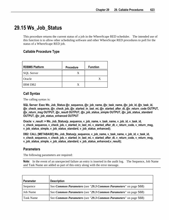
Chapter 29 29. Callable Procedures 623
29.15 Ws_Job_Status
This procedure returns the current status of a job in the WhereScape RED scheduler. The intended use of
this function is to allow other scheduling software and other WhereScape RED procedures to poll for the
status of a WhereScape RED job.
Callable Procedure Type
RDBMS Platform Procedure Function
SQL Server X
Oracle X
IBM DB2 X
Call Syntax
The calling syntax is:
SQL Server: Exec Ws_Job_Status @v_sequence, @v_job_name, @v_task_name, @v_job_id, @v_task_id, @v_check_sequence, @v_check_job, @v_started_in_last_mi, @v_started_after_dt, @v_return_code OUTPUT, @v_return_msg OUTPUT, @v_result OUTPUT, @v_job_status_simple OUTPUT, @v_job_status_standard OUTPUT, @v_job_status_enhanced OUTPUT
Oracle: v_result := Ws_Job_Status(p_sequence, v_job_name, v_task_name, v_job_id, v_task_id, v_check_sequence, v_check_job, v_started_in_last_mi, v_started_after_dt, v_return_code, v_return_msg, v_job_status_simple, v_job_status_standard, v_job_status_enhanced);
DB2: CALL [METABASE].Ws_Job_Status(p_sequence, v_job_name, v_task_name, v_job_id, v_task_id, v_check_sequence, v_check_job, v_started_in_last_mi, v_started_after_dt, v_return_code, v_return_msg, v_job_status_simple, v_job_status_standard, v_job_status_enhanced,v_result);
Parameters
The following parameters are required:
Note: In the event of an unexpected failure an entry is inserted in the audit log. The Sequence, Job Name
and Task Name are added as part of this entry along with the error message.
Parameter Description
Sequence See Common Parameters (see "29.3 Common Parameters" on page 568)
Job Name See Common Parameters (see "29.3 Common Parameters" on page 568)
Task Name See Common Parameters (see "29.3 Common Parameters" on page 568)
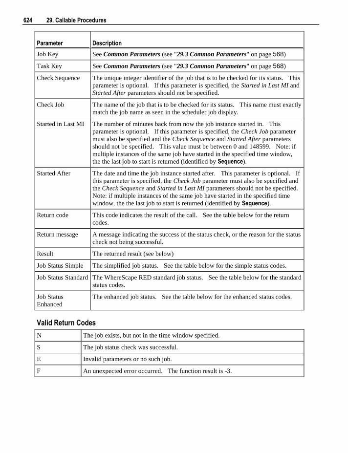
624 29. Callable Procedures
Parameter Description
Job Key See Common Parameters (see "29.3 Common Parameters" on page 568)
Task Key See Common Parameters (see "29.3 Common Parameters" on page 568)
Check Sequence The unique integer identifier of the job that is to be checked for its status. This
parameter is optional. If this parameter is specified, the Started in Last MI and
Started After parameters should not be specified.
Check Job The name of the job that is to be checked for its status. This name must exactly
match the job name as seen in the scheduler job display.
Started in Last MI The number of minutes back from now the job instance started in. This
parameter is optional. If this parameter is specified, the Check Job parameter
must also be specified and the Check Sequence and Started After parameters
should not be specified. This value must be between 0 and 148599. Note: if
multiple instances of the same job have started in the specified time window,
the the last job to start is returned (identified by Sequence).
Started After The date and time the job instance started after. This parameter is optional. If
this parameter is specified, the Check Job parameter must also be specified and
the Check Sequence and Started in Last MI parameters should not be specified.
Note: if multiple instances of the same job have started in the specified time
window, the the last job to start is returned (identified by Sequence).
Return code This code indicates the result of the call. See the table below for the return
codes.
Return message A message indicating the success of the status check, or the reason for the status
check not being successful.
Result The returned result (see below)
Job Status Simple The simplified job status. See the table below for the simple status codes.
Job Status Standard The WhereScape RED standard job status. See the table below for the standard
status codes.
Job Status
Enhanced
The enhanced job status. See the table below for the enhanced status codes.
Valid Return Codes
N The job exists, but not in the time window specified.
S The job status check was successful.
E Invalid parameters or no such job.
F An unexpected error occurred. The function result is -3.
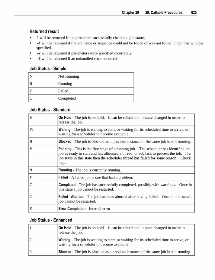
Chapter 29 29. Callable Procedures 625
Returned result
1 will be returned if the procedure successfully check the job status.
–1 will be returned if the job name or sequence could not be found or was not found in the time window
specified.
–2 will be returned if parameters were specified incorrectly.
–3 will be returned if an unhandled error occurred.
Job Status - Simple
N Not Running
R Running
F Failed
C Completed
Job Status - Standard
H On Hold - The job is on hold. It can be edited and its state changed in order to
release the job.
W Waiting - The job is waiting to start, or waiting for its scheduled time to arrive, or
waiting for a scheduler to become available.
B Blocked - The job is blocked as a previous instance of the same job is still running.
P Pending - This is the first stage of a running job. The scheduler has identified the
job as ready to start and has allocated a thread, or sub task to process the job. If a
job stays in this state then the scheduler thread has failed for some reason. Check
logs.
R Running - The job is currently running.
F Failed - A failed job is one that had a problem.
C Completed - The job has successfully completed, possibly with warnings. Once in
this state a job cannot be restarted.
G Failed - Aborted - The job has been aborted after having failed. Once in this state a
job cannot be restarted.
E Error Completion - Internal error.
Job Status - Enhanced
1 On Hold - The job is on hold. It can be edited and its state changed in order to
release the job.
2 Waiting - The job is waiting to start, or waiting for its scheduled time to arrive, or
waiting for a scheduler to become available.
3 Blocked - The job is blocked as a previous instance of the same job is still running.

626 29. Callable Procedures
4 Pending - This is the first stage of a running job. The scheduler has identified the
job as ready to start and has allocated a thread, or sub task to process the job. If a
job stays in this state then the scheduler thread has failed for some reason. Check
logs.
5 Running - The job is currently running, no tasks have failed and there are no
warnings.
6 Running with Errors - The job is currently running and some completed tasks have
failed. When all tasks not dependent on the failed tasks have completed, the job
will fail.
7 Running with Warnings - The job is currently running and some tasks have
warnings.
8 Failed - A failed job is one that had a problem.
9 Completed - The job has successfully completed, without warnings. Once in this
state a job cannot be restarted.
10 Completed with Warnings - The job has successfully completed, with warnings.
Once in this state a job cannot be restarted.
11 Failed - Aborted - The job has been aborted after having failed. Once in this state a
job cannot be restarted.
12 Error Completion - Internal error.
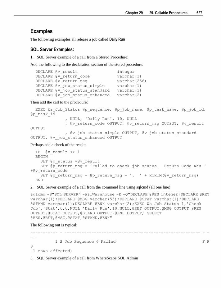
Chapter 29 29. Callable Procedures 627
Examples
The following examples all release a job called Daily Run
SQL Server Examples:
1. SQL Server example of a call from a Stored Procedure:
Add the following to the declaration section of the stored procedure:
DECLARE @v_result integer
DECLARE @v_return_code varchar(1)
DECLARE @v_return_msg varchar(256)
DECLARE @v_job_status_simple varchar(1)
DECLARE @v_job_status_standard varchar(1)
DECLARE @v_job_status_enhanced varchar(2)
Then add the call to the procedure:
EXEC Ws_Job_Status @p_sequence, @p_job_name, @p_task_name, @p_job_id,
@p_task_id
, NULL, 'Daily Run', 10, NULL
, @v_return_code OUTPUT, @v_return_msg OUTPUT, @v_result
OUTPUT
, @v_job_status_simple OUTPUT, @v_job_status_standard
OUTPUT, @v_job_status_enhanced OUTPUT
Perhaps add a check of the result:
IF @v_result <> 1
BEGIN
SET @p_status =@v_result
SET @p_return_msg = 'Failed to check job status. Return Code was '
+@v_return_code
SET @p_return_msg = @p_return_msg + '. ' + RTRIM(@v_return_msg)
END
2. SQL Server example of a call from the command line using sqlcmd (all one line):
sqlcmd -S"SQL SERVER" -WslWarehouse -E -Q"DECLARE @RES integer;DECLARE @RET
varchar(1);DECLARE @MSG varchar(55);DECLARE @STAT varchar(1);DECLARE
@STAND varchar(1);DECLARE @ENH varchar(2);EXEC Ws_Job_Status 1,'Check
Job','Stat',0,0,NULL,'Daily Run',10,NULL,@RET OUTPUT,@MSG OUTPUT,@RES
OUTPUT,@STAT OUTPUT,@STAND OUTPUT,@ENH OUTPUT; SELECT
@RES,@RET,@MSG,@STAT,@STAND,@ENH"
The following out is typical:
----------- - ------------------------------------------------------- - -
--
1 S Job Sequence 6 Failed F F
8
(1 rows affected)
3. SQL Server example of a call from WhereScape SQL Admin
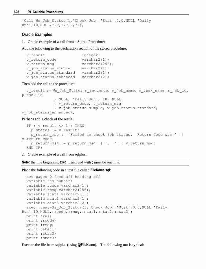
628 29. Callable Procedures
{Call Ws_Job_Status(1,'Check Job','Stat',0,0,NULL,'Daily
Run',10,NULL,?,?,?,?,?,?)};
Oracle Examples:
1. Oracle example of a call from a Stored Procedure:
Add the following to the declaration section of the stored procedure:
v_result integer;
v_return_code varchar2(1);
v_return_msg varchar2(256);
v_job_status_simple varchar2(1);
v_job_status_standard varchar2(1);
v_job_status_enhanced varchar2(2);
Then add the call to the procedure:
v_result := Ws_Job_Status(p_sequence, p_job_name, p_task_name, p_job_id,
p_task_id
, NULL, 'Daily Run', 10, NULL
, v_return_code, v_return_msg
, v_job_status_simple, v_job_status_standard,
v_job_status_enhanced);
Perhaps add a check of the result:
IF ( v_result <> 1 ) THEN
p_status := v_result;
p_return_msg := 'Failed to check job status. Return Code was ' ||
v_return_code;
p_return_msg := p_return_msg || '. ' || v_return_msg;
END IF;
2. Oracle example of a call from sqlplus:
Note: the line beginning exec ... and end with ; must be one line.
Place the following code in a text file called FileName.sql:
set pages 0 feed off heading off
variable res number;
variable rcode varchar2(1);
variable rmsg varchar2(256);
variable stat1 varchar2(1);
variable stat2 varchar2(1);
variable stat3 varchar2(2);
exec :res:=Ws_Job_Status(1,'Check Job','Stat',0,0,NULL,'Daily
Run',10,NULL,:rcode,:rmsg,:stat1,:stat2,:stat3);
print :res;
print :rcode;
print :rmsg;
print :stat1;
print :stat2;
print :stat3;
Execute the file from sqlplus (using @FileName). The following out is typical:
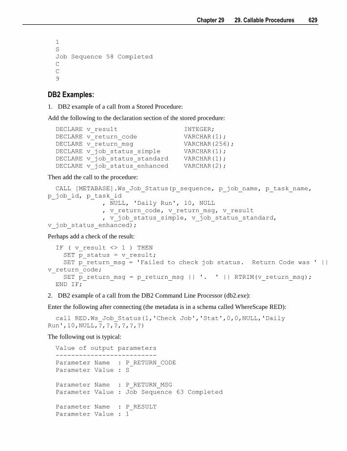
Chapter 29 29. Callable Procedures 629
1
S
Job Sequence 58 Completed
C
C
9
DB2 Examples:
1. DB2 example of a call from a Stored Procedure:
Add the following to the declaration section of the stored procedure:
DECLARE v_result INTEGER;
DECLARE v_return_code VARCHAR(1);
DECLARE v_return_msg VARCHAR(256);
DECLARE v_job_status_simple VARCHAR(1);
DECLARE v_job_status_standard VARCHAR(1);
DECLARE v_job_status_enhanced VARCHAR(2);
Then add the call to the procedure:
CALL [METABASE].Ws_Job_Status(p_sequence, p_job_name, p_task_name,
p_job_id, p_task_id
, NULL, 'Daily Run', 10, NULL
, v_return_code, v_return_msg, v_result
, v_job_status_simple, v_job_status_standard,
v_job_status_enhanced);
Perhaps add a check of the result:
IF ( v_result <> 1 ) THEN
SET p_status = v_result;
SET p_return_msg = 'Failed to check job status. Return Code was ' ||
v_return_code;
SET p_return_msg = p_return_msg || '. ' || RTRIM(v_return_msg);
END IF;
2. DB2 example of a call from the DB2 Command Line Processor (db2.exe):
Enter the following after connecting (the metadata is in a schema called WhereScape RED):
call RED.Ws_Job_Status(1,'Check Job','Stat',0,0,NULL,'Daily
Run',10,NULL,?,?,?,?,?,?)
The following out is typical:
Value of output parameters
--------------------------
Parameter Name : P_RETURN_CODE
Parameter Value : S
Parameter Name : P_RETURN_MSG
Parameter Value : Job Sequence 63 Completed
Parameter Name : P_RESULT
Parameter Value : 1
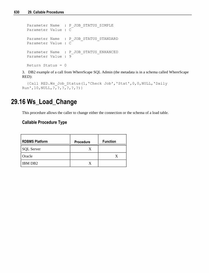
630 29. Callable Procedures
Parameter Name : P_JOB_STATUS_SIMPLE
Parameter Value : C
Parameter Name : P_JOB_STATUS_STANDARD
Parameter Value : C
Parameter Name : P_JOB_STATUS_ENHANCED
Parameter Value : 9
Return Status = 0
3. DB2 example of a call from WhereScape SQL Admin (the metadata is in a schema called WhereScape
RED):
{Call RED.Ws_Job_Status(1,'Check Job','Stat',0,0,NULL,'Daily
Run',10,NULL,?,?,?,?,?,?)}
29.16 Ws_Load_Change
This procedure allows the caller to change either the connection or the schema of a load table.
Callable Procedure Type
RDBMS Platform Procedure Function
SQL Server X
Oracle X
IBM DB2 X
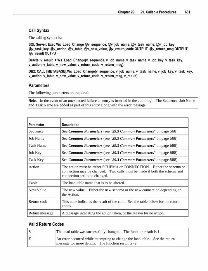
Chapter 29 29. Callable Procedures 631
Call Syntax
The calling syntax is:
SQL Server: Exec Ws_Load_Change @v_sequence, @v_job_name, @v_task_name, @v_job_key, @v_task_key, @v_action, @v_table, @v_new_value, @v_return_code OUTPUT, @v_return_msg OUTPUT, @v_result OUTPUT
Oracle: v_result := Ws_Load_Change(v_sequence, v_job_name, v_task_name, v_job_key, v_task_key, v_action, v_table, v_new_value, v_return_code, v_return_msg);
DB2: CALL [METABASE].Ws_Load_Change(v_sequence, v_job_name, v_task_name, v_job_key, v_task_key, v_action, v_table, v_new_value, v_return_code, v_return_msg, v_result);
Parameters
The following parameters are required:
Note: In the event of an unexpected failure an entry is inserted in the audit log. The Sequence, Job Name
and Task Name are added as part of this entry along with the error message.
Parameter Description
Sequence See Common Parameters (see "29.3 Common Parameters" on page 568)
Job Name See Common Parameters (see "29.3 Common Parameters" on page 568)
Task Name See Common Parameters (see "29.3 Common Parameters" on page 568)
Job Key See Common Parameters (see "29.3 Common Parameters" on page 568)
Task Key See Common Parameters (see "29.3 Common Parameters" on page 568)
Action The action must be either SCHEMA or CONNECTION. Either the schema or
connection may be changed. Two calls must be made if both the schema and
connection are to be changed.
Table The load table name that is to be altered.
New Value The new value. Either the new schema or the new connection depending on
the Action.
Return code This code indicates the result of the call. See the table below for the return
codes.
Return message A message indicating the action taken, or the reason for no action.
Valid Return Codes
S The load table was successfully changed. The function result is 1.
E An error occurred while attempting to change the load table. See the return
message for more details. The function result is -2.
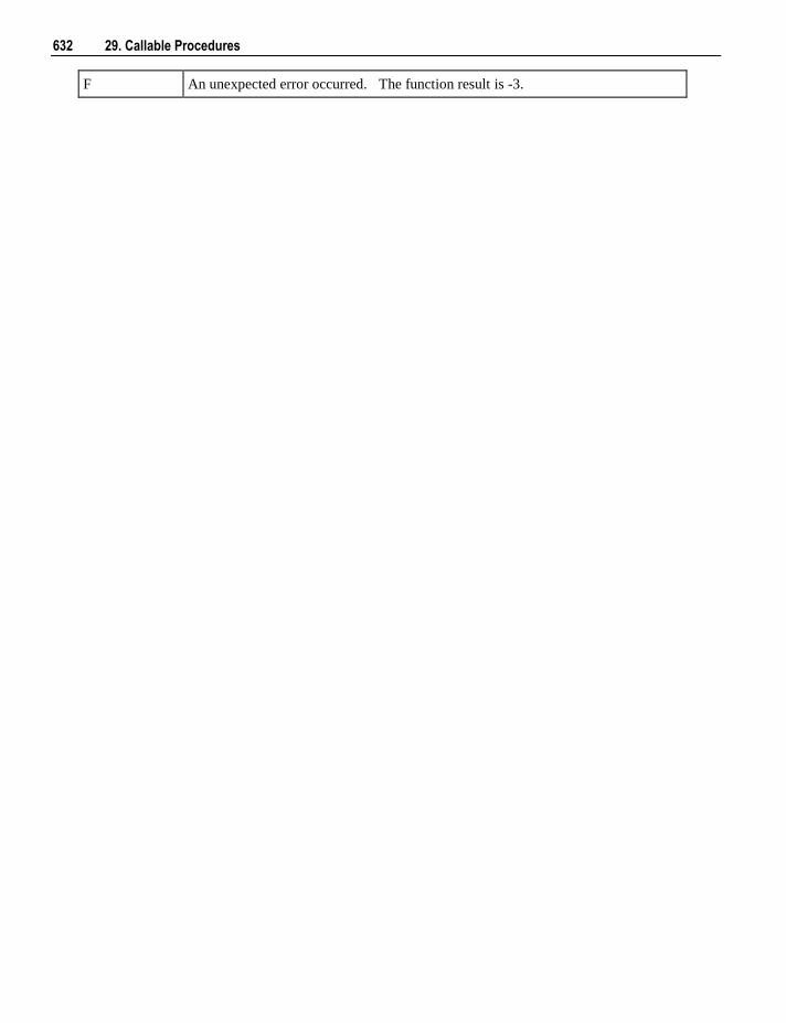
632 29. Callable Procedures
F An unexpected error occurred. The function result is -3.
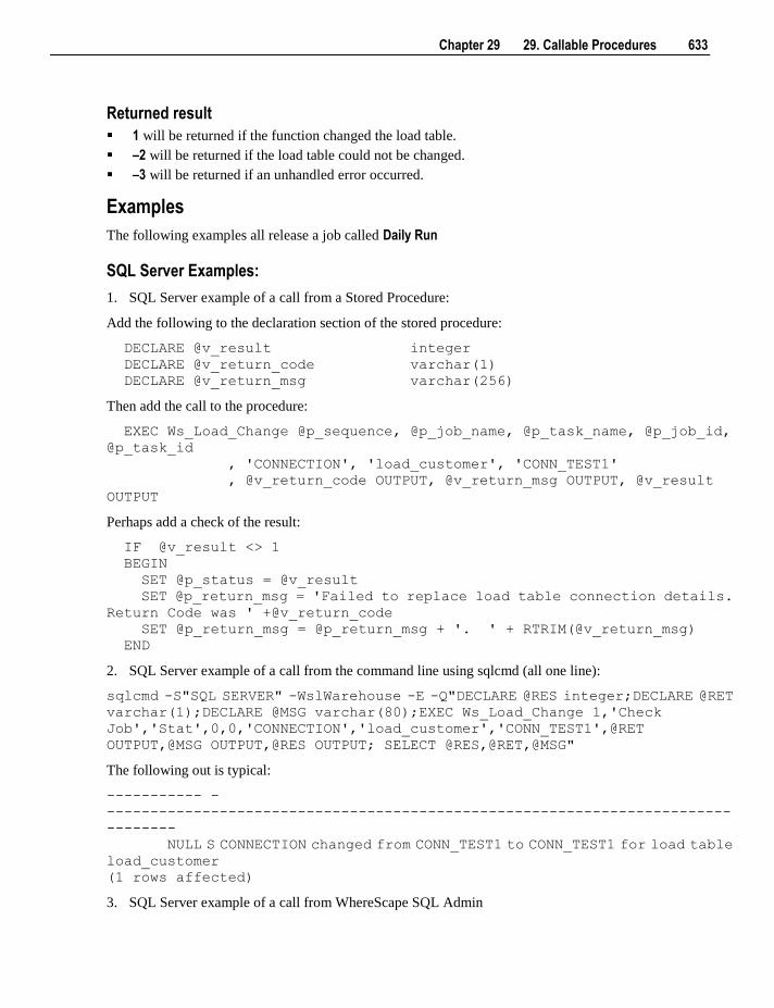
Chapter 29 29. Callable Procedures 633
Returned result
1 will be returned if the function changed the load table.
–2 will be returned if the load table could not be changed.
–3 will be returned if an unhandled error occurred.
Examples
The following examples all release a job called Daily Run
SQL Server Examples:
1. SQL Server example of a call from a Stored Procedure:
Add the following to the declaration section of the stored procedure:
DECLARE @v_result integer
DECLARE @v_return_code varchar(1)
DECLARE @v_return_msg varchar(256)
Then add the call to the procedure:
EXEC Ws_Load_Change @p_sequence, @p_job_name, @p_task_name, @p_job_id,
@p_task_id
, 'CONNECTION', 'load_customer', 'CONN_TEST1'
, @v_return_code OUTPUT, @v_return_msg OUTPUT, @v_result
OUTPUT
Perhaps add a check of the result:
IF @v_result <> 1
BEGIN
SET @p_status = @v_result
SET @p_return_msg = 'Failed to replace load table connection details.
Return Code was ' +@v_return_code
SET @p_return_msg = @p_return_msg + '. ' + RTRIM(@v_return_msg)
END
2. SQL Server example of a call from the command line using sqlcmd (all one line):
sqlcmd -S"SQL SERVER" -WslWarehouse -E -Q"DECLARE @RES integer;DECLARE @RET
varchar(1);DECLARE @MSG varchar(80);EXEC Ws_Load_Change 1,'Check
Job','Stat',0,0,'CONNECTION','load_customer','CONN_TEST1',@RET
OUTPUT,@MSG OUTPUT,@RES OUTPUT; SELECT @RES,@RET,@MSG"
The following out is typical:
----------- -
------------------------------------------------------------------------
--------
NULL S CONNECTION changed from CONN_TEST1 to CONN_TEST1 for load table
load_customer
(1 rows affected)
3. SQL Server example of a call from WhereScape SQL Admin
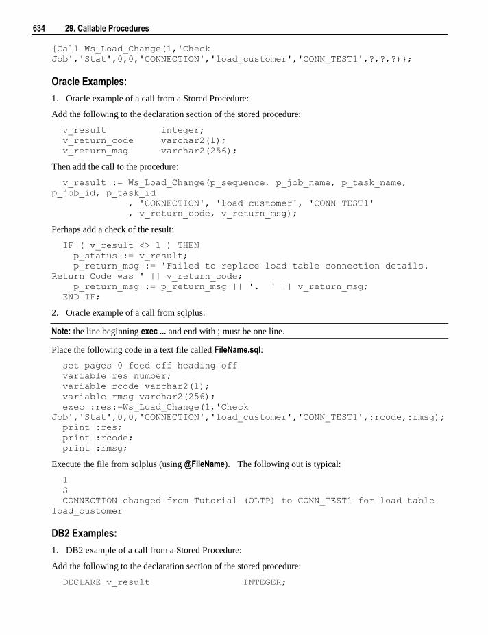
634 29. Callable Procedures
{Call Ws_Load_Change(1,'Check
Job','Stat',0,0,'CONNECTION','load_customer','CONN_TEST1',?,?,?)};
Oracle Examples:
1. Oracle example of a call from a Stored Procedure:
Add the following to the declaration section of the stored procedure:
v_result integer;
v_return_code varchar2(1);
v_return_msg varchar2(256);
Then add the call to the procedure:
v_result := Ws_Load_Change(p_sequence, p_job_name, p_task_name,
p_job_id, p_task_id
, 'CONNECTION', 'load_customer', 'CONN_TEST1'
, v_return_code, v_return_msg);
Perhaps add a check of the result:
IF ( v_result <> 1 ) THEN
p_status := v_result;
p_return_msg := 'Failed to replace load table connection details.
Return Code was ' || v_return_code;
p_return_msg := p_return_msg || '. ' || v_return_msg;
END IF;
2. Oracle example of a call from sqlplus:
Note: the line beginning exec ... and end with ; must be one line.
Place the following code in a text file called FileName.sql:
set pages 0 feed off heading off
variable res number;
variable rcode varchar2(1);
variable rmsg varchar2(256);
exec :res:=Ws_Load_Change(1,'Check
Job','Stat',0,0,'CONNECTION','load_customer','CONN_TEST1',:rcode,:rmsg);
print :res;
print :rcode;
print :rmsg;
Execute the file from sqlplus (using @FileName). The following out is typical:
1
S
CONNECTION changed from Tutorial (OLTP) to CONN_TEST1 for load table
load_customer
DB2 Examples:
1. DB2 example of a call from a Stored Procedure:
Add the following to the declaration section of the stored procedure:
DECLARE v_result INTEGER;
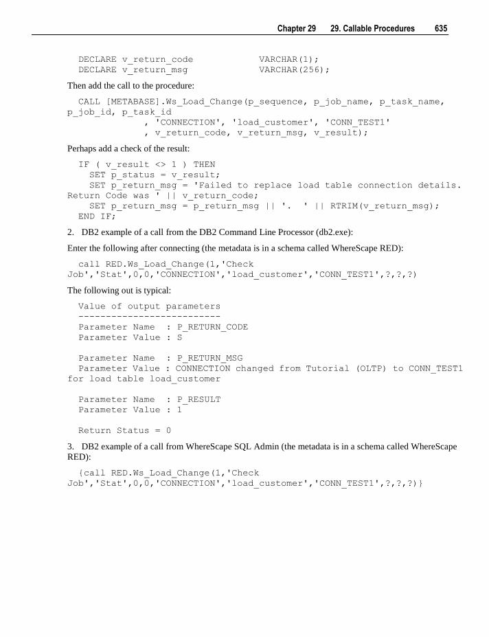
Chapter 29 29. Callable Procedures 635
DECLARE v_return_code VARCHAR(1);
DECLARE v_return_msg VARCHAR(256);
Then add the call to the procedure:
CALL [METABASE].Ws_Load_Change(p_sequence, p_job_name, p_task_name,
p_job_id, p_task_id
, 'CONNECTION', 'load_customer', 'CONN_TEST1'
, v_return_code, v_return_msg, v_result);
Perhaps add a check of the result:
IF ( v_result <> 1 ) THEN
SET p_status = v_result;
SET p_return_msg = 'Failed to replace load table connection details.
Return Code was ' || v_return_code;
SET p_return_msg = p_return_msg || '. ' || RTRIM(v_return_msg);
END IF;
2. DB2 example of a call from the DB2 Command Line Processor (db2.exe):
Enter the following after connecting (the metadata is in a schema called WhereScape RED):
call RED.Ws_Load_Change(1,'Check
Job','Stat',0,0,'CONNECTION','load_customer','CONN_TEST1',?,?,?)
The following out is typical:
Value of output parameters
--------------------------
Parameter Name : P_RETURN_CODE
Parameter Value : S
Parameter Name : P_RETURN_MSG
Parameter Value : CONNECTION changed from Tutorial (OLTP) to CONN_TEST1
for load table load_customer
Parameter Name : P_RESULT
Parameter Value : 1
Return Status = 0
3. DB2 example of a call from WhereScape SQL Admin (the metadata is in a schema called WhereScape
RED):
{call RED.Ws_Load_Change(1,'Check
Job','Stat',0,0,'CONNECTION','load_customer','CONN_TEST1',?,?,?)}
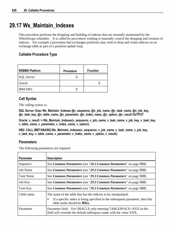
636 29. Callable Procedures
29.17 Ws_Maintain_Indexes
This procedure performs the dropping and building of indexes that are normally maintained by the
WhereScape scheduler. It is called by procedures wishing to manually control the dropping and creation of
indexes. For example a procedure that exchanges partitions may wish to drop and create indexes on an
exchange table as part of a partition update loop.
Callable Procedure Type
RDBMS Platform Procedure Function
SQL Server X
Oracle X
IBM DB2 X
Call Syntax
The calling syntax is:
SQL Server: Exec Ws_Maintain_Indexes @v_sequence, @v_job_name, @v_task_name, @v_job_key, @v_task_key, @v_table_name, @v_parameter, @v_index_name, @v_option, @v_result OUTPUT
Oracle: v_result := Ws_Maintain_Indexes(v_sequence, v_job_name, v_task_name, v_job_key, v_task_key, v_table_name, v_parameter, v_index_name, v_option);
DB2: CALL [METABASE].Ws_Maintain_Indexes(v_sequence, v_job_name, v_task_name, v_job_key, v_task_key, v_table_name, v_parameter, v_index_name, v_option, v_result);
Parameters
The following parameters are required:
Parameter Description
Sequence See Common Parameters (see "29.3 Common Parameters" on page 568)
Job Name See Common Parameters (see "29.3 Common Parameters" on page 568)
Task Name See Common Parameters (see "29.3 Common Parameters" on page 568)
Job Key See Common Parameters (see "29.3 Common Parameters" on page 568)
Task Key See Common Parameters (see "29.3 Common Parameters" on page 568)
Table name The name of the table that has the indexes to be manipulated.
If a specific index is being specified in the subsequent parameter, then this
table name should be NULL.
Parameter Parameter field. For ORACLE only entering TABLESPACE=XXX in this
field will override the default tablespace name with the value XXX.
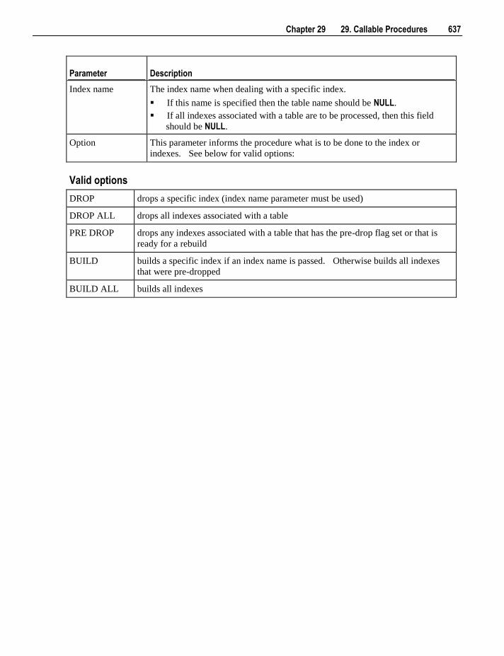
Chapter 29 29. Callable Procedures 637
Parameter Description
Index name The index name when dealing with a specific index.
If this name is specified then the table name should be NULL.
If all indexes associated with a table are to be processed, then this field
should be NULL.
Option This parameter informs the procedure what is to be done to the index or
indexes. See below for valid options:
Valid options
DROP drops a specific index (index name parameter must be used)
DROP ALL drops all indexes associated with a table
PRE DROP drops any indexes associated with a table that has the pre-drop flag set or that is
ready for a rebuild
BUILD builds a specific index if an index name is passed. Otherwise builds all indexes
that were pre-dropped
BUILD ALL builds all indexes
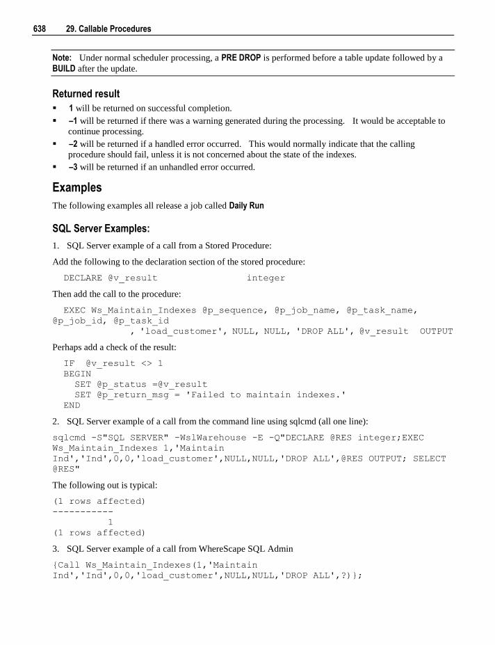
638 29. Callable Procedures
Note: Under normal scheduler processing, a PRE DROP is performed before a table update followed by a
BUILD after the update.
Returned result
1 will be returned on successful completion.
–1 will be returned if there was a warning generated during the processing. It would be acceptable to
continue processing.
–2 will be returned if a handled error occurred. This would normally indicate that the calling
procedure should fail, unless it is not concerned about the state of the indexes.
–3 will be returned if an unhandled error occurred.
Examples
The following examples all release a job called Daily Run
SQL Server Examples:
1. SQL Server example of a call from a Stored Procedure:
Add the following to the declaration section of the stored procedure:
DECLARE @v_result integer
Then add the call to the procedure:
EXEC Ws_Maintain_Indexes @p_sequence, @p_job_name, @p_task_name,
@p_job_id, @p_task_id
, 'load_customer', NULL, NULL, 'DROP ALL', @v_result OUTPUT
Perhaps add a check of the result:
IF @v_result <> 1
BEGIN
SET @p_status =@v_result
SET @p_return_msg = 'Failed to maintain indexes.'
END
2. SQL Server example of a call from the command line using sqlcmd (all one line):
sqlcmd -S"SQL SERVER" -WslWarehouse -E -Q"DECLARE @RES integer;EXEC
Ws_Maintain_Indexes 1,'Maintain
Ind','Ind',0,0,'load_customer',NULL,NULL,'DROP ALL',@RES OUTPUT; SELECT
@RES"
The following out is typical:
(1 rows affected)
-----------
1
(1 rows affected)
3. SQL Server example of a call from WhereScape SQL Admin
{Call Ws_Maintain_Indexes(1,'Maintain
Ind','Ind',0,0,'load_customer',NULL,NULL,'DROP ALL',?)};
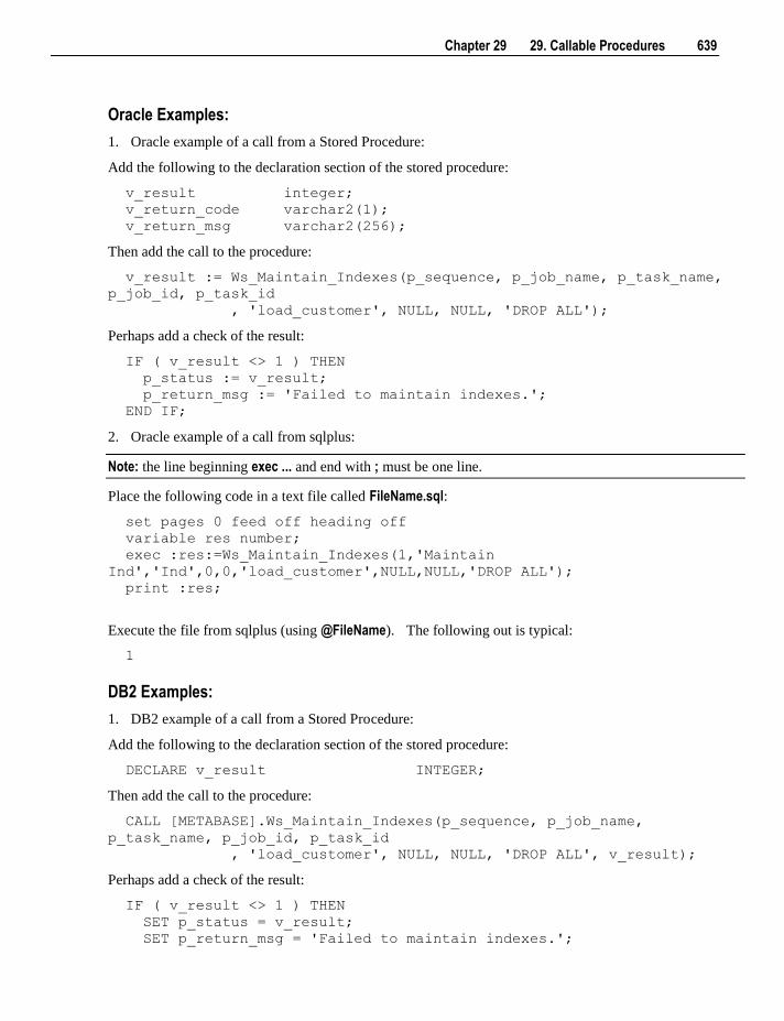
Chapter 29 29. Callable Procedures 639
Oracle Examples:
1. Oracle example of a call from a Stored Procedure:
Add the following to the declaration section of the stored procedure:
v_result integer;
v_return_code varchar2(1);
v_return_msg varchar2(256);
Then add the call to the procedure:
v_result := Ws_Maintain_Indexes(p_sequence, p_job_name, p_task_name,
p_job_id, p_task_id
, 'load_customer', NULL, NULL, 'DROP ALL');
Perhaps add a check of the result:
IF ( v_result <> 1 ) THEN
p_status := v_result;
p_return_msg := 'Failed to maintain indexes.';
END IF;
2. Oracle example of a call from sqlplus:
Note: the line beginning exec ... and end with ; must be one line.
Place the following code in a text file called FileName.sql:
set pages 0 feed off heading off
variable res number;
exec :res:=Ws_Maintain_Indexes(1,'Maintain
Ind','Ind',0,0,'load_customer',NULL,NULL,'DROP ALL');
print :res;
Execute the file from sqlplus (using @FileName). The following out is typical:
1
DB2 Examples:
1. DB2 example of a call from a Stored Procedure:
Add the following to the declaration section of the stored procedure:
DECLARE v_result INTEGER;
Then add the call to the procedure:
CALL [METABASE].Ws_Maintain_Indexes(p_sequence, p_job_name,
p_task_name, p_job_id, p_task_id
, 'load_customer', NULL, NULL, 'DROP ALL', v_result);
Perhaps add a check of the result:
IF ( v_result <> 1 ) THEN
SET p_status = v_result;
SET p_return_msg = 'Failed to maintain indexes.';
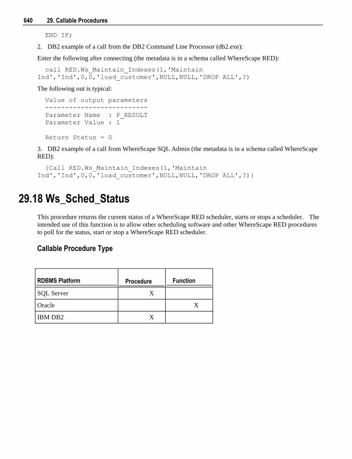
640 29. Callable Procedures
END IF;
2. DB2 example of a call from the DB2 Command Line Processor (db2.exe):
Enter the following after connecting (the metadata is in a schema called WhereScape RED):
call RED.Ws_Maintain_Indexes(1,'Maintain
Ind','Ind',0,0,'load_customer',NULL,NULL,'DROP ALL',?)
The following out is typical:
Value of output parameters
--------------------------
Parameter Name : P_RESULT
Parameter Value : 1
Return Status = 0
3. DB2 example of a call from WhereScape SQL Admin (the metadata is in a schema called WhereScape
RED):
{Call RED.Ws_Maintain_Indexes(1,'Maintain
Ind','Ind',0,0,'load_customer',NULL,NULL,'DROP ALL',?)}
29.18 Ws_Sched_Status
This procedure returns the current status of a WhereScape RED scheduler, starts or stops a scheduler. The
intended use of this function is to allow other scheduling software and other WhereScape RED procedures
to poll for the status, start or stop a WhereScape RED scheduler.
Callable Procedure Type
RDBMS Platform Procedure Function
SQL Server X
Oracle X
IBM DB2 X
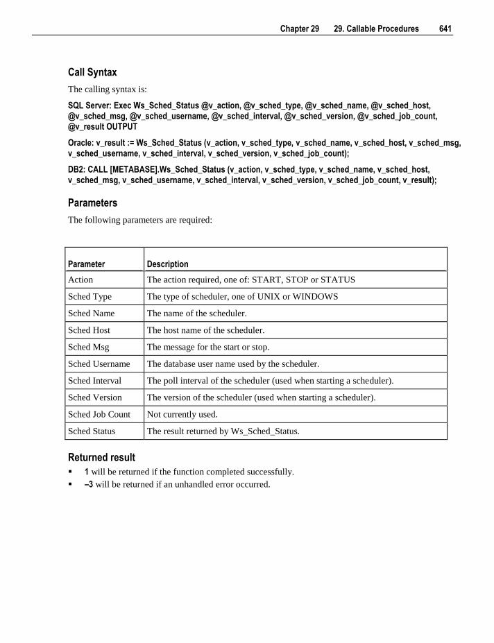
Chapter 29 29. Callable Procedures 641
Call Syntax
The calling syntax is:
SQL Server: Exec Ws_Sched_Status @v_action, @v_sched_type, @v_sched_name, @v_sched_host, @v_sched_msg, @v_sched_username, @v_sched_interval, @v_sched_version, @v_sched_job_count, @v_result OUTPUT
Oracle: v_result := Ws_Sched_Status (v_action, v_sched_type, v_sched_name, v_sched_host, v_sched_msg, v_sched_username, v_sched_interval, v_sched_version, v_sched_job_count);
DB2: CALL [METABASE].Ws_Sched_Status (v_action, v_sched_type, v_sched_name, v_sched_host, v_sched_msg, v_sched_username, v_sched_interval, v_sched_version, v_sched_job_count, v_result);
Parameters
The following parameters are required:
Parameter Description
Action The action required, one of: START, STOP or STATUS
Sched Type The type of scheduler, one of UNIX or WINDOWS
Sched Name The name of the scheduler.
Sched Host The host name of the scheduler.
Sched Msg The message for the start or stop.
Sched Username The database user name used by the scheduler.
Sched Interval The poll interval of the scheduler (used when starting a scheduler).
Sched Version The version of the scheduler (used when starting a scheduler).
Sched Job Count Not currently used.
Sched Status The result returned by Ws_Sched_Status.
Returned result
1 will be returned if the function completed successfully.
–3 will be returned if an unhandled error occurred.
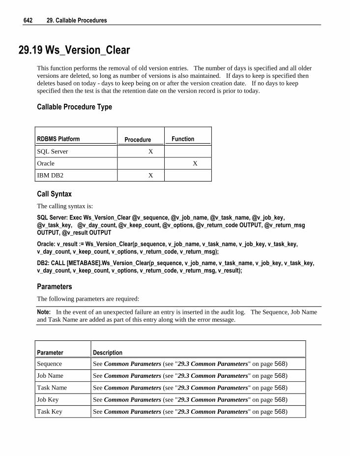
642 29. Callable Procedures
29.19 Ws_Version_Clear
This function performs the removal of old version entries. The number of days is specified and all older
versions are deleted, so long as number of versions is also maintained. If days to keep is specified then
deletes based on today - days to keep being on or after the version creation date. If no days to keep
specified then the test is that the retention date on the version record is prior to today.
Callable Procedure Type
RDBMS Platform Procedure Function
SQL Server X
Oracle X
IBM DB2 X
Call Syntax
The calling syntax is:
SQL Server: Exec Ws_Version_Clear @v_sequence, @v_job_name, @v_task_name, @v_job_key, @v_task_key, @v_day_count, @v_keep_count, @v_options, @v_return_code OUTPUT, @v_return_msg OUTPUT, @v_result OUTPUT
Oracle: v_result := Ws_Version_Clear(p_sequence, v_job_name, v_task_name, v_job_key, v_task_key, v_day_count, v_keep_count, v_options, v_return_code, v_return_msg);
DB2: CALL [METABASE].Ws_Version_Clear(p_sequence, v_job_name, v_task_name, v_job_key, v_task_key, v_day_count, v_keep_count, v_options, v_return_code, v_return_msg, v_result);
Parameters
The following parameters are required:
Note: In the event of an unexpected failure an entry is inserted in the audit log. The Sequence, Job Name
and Task Name are added as part of this entry along with the error message.
Parameter Description
Sequence See Common Parameters (see "29.3 Common Parameters" on page 568)
Job Name See Common Parameters (see "29.3 Common Parameters" on page 568)
Task Name See Common Parameters (see "29.3 Common Parameters" on page 568)
Job Key See Common Parameters (see "29.3 Common Parameters" on page 568)
Task Key See Common Parameters (see "29.3 Common Parameters" on page 568)
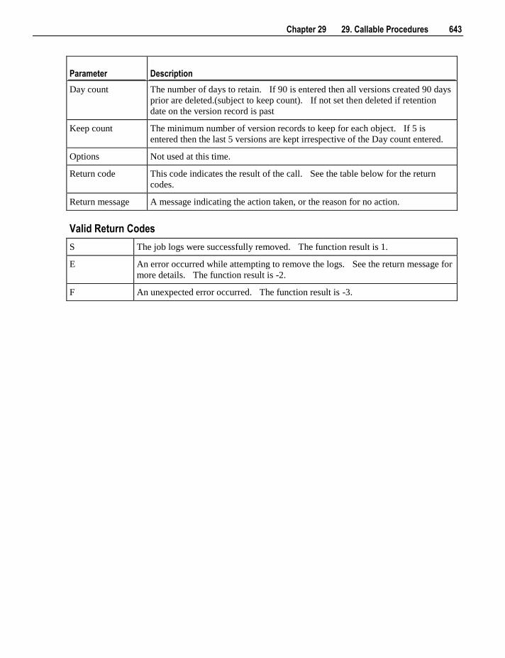
Chapter 29 29. Callable Procedures 643
Parameter Description
Day count The number of days to retain. If 90 is entered then all versions created 90 days
prior are deleted.(subject to keep count). If not set then deleted if retention
date on the version record is past
Keep count The minimum number of version records to keep for each object. If 5 is
entered then the last 5 versions are kept irrespective of the Day count entered.
Options Not used at this time.
Return code This code indicates the result of the call. See the table below for the return
codes.
Return message A message indicating the action taken, or the reason for no action.
Valid Return Codes
S The job logs were successfully removed. The function result is 1.
E An error occurred while attempting to remove the logs. See the return message for
more details. The function result is -2.
F An unexpected error occurred. The function result is -3.
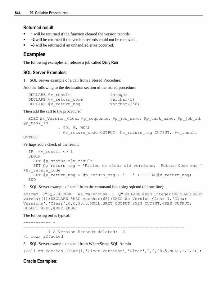
644 29. Callable Procedures
Returned result
1 will be returned if the function cleared the version records.
–2 will be returned if the version records could not be removed..
–3 will be returned if an unhandled error occurred.
Examples
The following examples all release a job called Daily Run
SQL Server Examples:
1. SQL Server example of a call from a Stored Procedure:
Add the following to the declaration section of the stored procedure:
DECLARE @v_result integer
DECLARE @v_return_code varchar(1)
DECLARE @v_return_msg varchar(256)
Then add the call to the procedure:
EXEC Ws_Version_Clear @p_sequence, @p_job_name, @p_task_name, @p_job_id,
@p_task_id
, 90, 5, NULL
, @v_return_code OUTPUT, @v_return_msg OUTPUT, @v_result
OUTPUT
Perhaps add a check of the result:
IF @v_result <> 1
BEGIN
SET @p_status =@v_result
SET @p_return_msg = 'Failed to clear old versions. Return Code was '
+@v_return_code
SET @p_return_msg = @p_return_msg + '. ' + RTRIM(@v_return_msg)
END
2. SQL Server example of a call from the command line using sqlcmd (all one line):
sqlcmd -S"SQL SERVER" -WslWarehouse -E -Q"DECLARE @RES integer;DECLARE @RET
varchar(1);DECLARE @MSG varchar(65);EXEC Ws_Version_Clear 1,'Clear
Versions','Clear',0,0,90,5,NULL,@RET OUTPUT,@MSG OUTPUT,@RES OUTPUT;
SELECT @RES,@RET,@MSG"
The following out is typical:
----------- -
-----------------------------------------------------------------
1 S Version Records deleted: 0
(1 rows affected)
3. SQL Server example of a call from WhereScape SQL Admin
{Call Ws_Version_Clear(1,'Clear Versions','Clear',0,0,90,5,NULL,?,?,?)};
Oracle Examples:
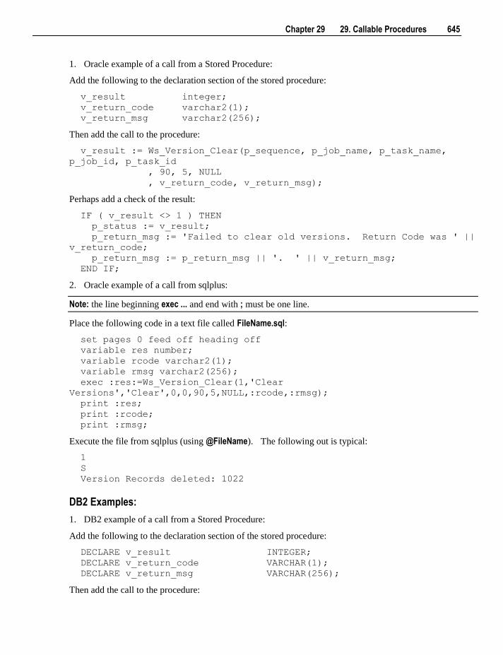
Chapter 29 29. Callable Procedures 645
1. Oracle example of a call from a Stored Procedure:
Add the following to the declaration section of the stored procedure:
v_result integer;
v_return_code varchar2(1);
v_return_msg varchar2(256);
Then add the call to the procedure:
v_result := Ws_Version_Clear(p_sequence, p_job_name, p_task_name,
p_job_id, p_task_id
, 90, 5, NULL
, v_return_code, v_return_msg);
Perhaps add a check of the result:
IF ( v_result <> 1 ) THEN
p_status := v_result;
p_return_msg := 'Failed to clear old versions. Return Code was ' ||
v_return_code;
p_return_msg := p_return_msg || '. ' || v_return_msg;
END IF;
2. Oracle example of a call from sqlplus:
Note: the line beginning exec ... and end with ; must be one line.
Place the following code in a text file called FileName.sql:
set pages 0 feed off heading off
variable res number;
variable rcode varchar2(1);
variable rmsg varchar2(256);
exec :res:=Ws_Version_Clear(1,'Clear
Versions','Clear',0,0,90,5,NULL,:rcode,:rmsg);
print :res;
print :rcode;
print :rmsg;
Execute the file from sqlplus (using @FileName). The following out is typical:
1
S
Version Records deleted: 1022
DB2 Examples:
1. DB2 example of a call from a Stored Procedure:
Add the following to the declaration section of the stored procedure:
DECLARE v_result INTEGER;
DECLARE v_return_code VARCHAR(1);
DECLARE v_return_msg VARCHAR(256);
Then add the call to the procedure:
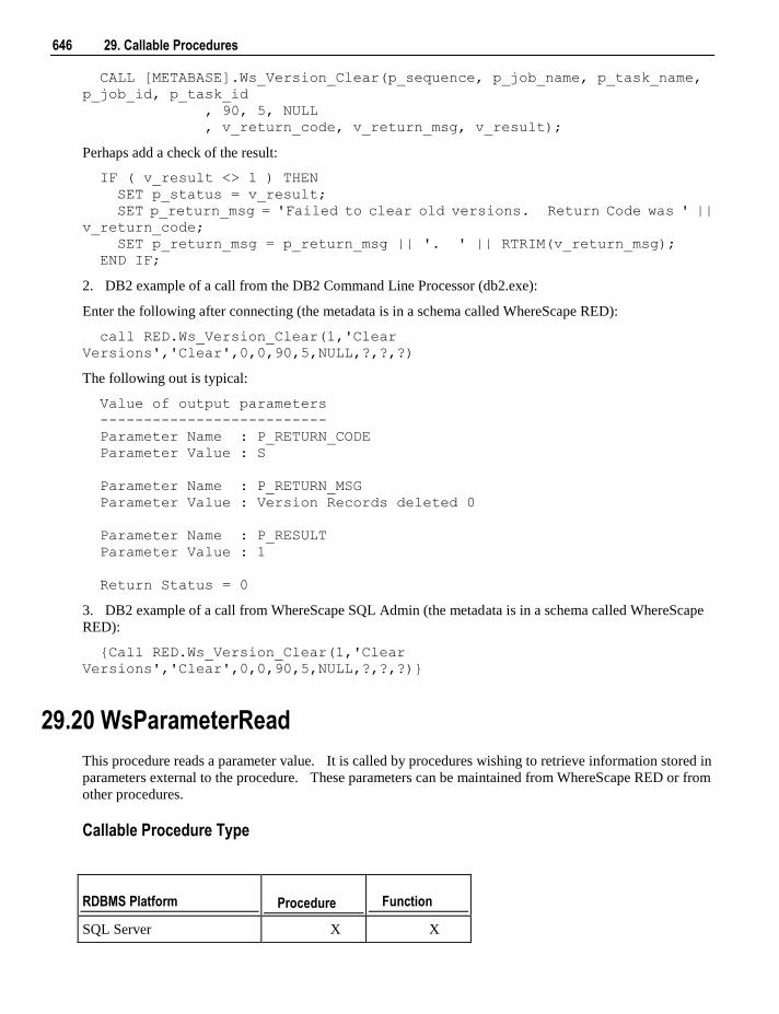
646 29. Callable Procedures
CALL [METABASE].Ws_Version_Clear(p_sequence, p_job_name, p_task_name,
p_job_id, p_task_id
, 90, 5, NULL
, v_return_code, v_return_msg, v_result);
Perhaps add a check of the result:
IF ( v_result <> 1 ) THEN
SET p_status = v_result;
SET p_return_msg = 'Failed to clear old versions. Return Code was ' ||
v_return_code;
SET p_return_msg = p_return_msg || '. ' || RTRIM(v_return_msg);
END IF;
2. DB2 example of a call from the DB2 Command Line Processor (db2.exe):
Enter the following after connecting (the metadata is in a schema called WhereScape RED):
call RED.Ws_Version_Clear(1,'Clear
Versions','Clear',0,0,90,5,NULL,?,?,?)
The following out is typical:
Value of output parameters
--------------------------
Parameter Name : P_RETURN_CODE
Parameter Value : S
Parameter Name : P_RETURN_MSG
Parameter Value : Version Records deleted 0
Parameter Name : P_RESULT
Parameter Value : 1
Return Status = 0
3. DB2 example of a call from WhereScape SQL Admin (the metadata is in a schema called WhereScape
RED):
{Call RED.Ws_Version_Clear(1,'Clear
Versions','Clear',0,0,90,5,NULL,?,?,?)}
29.20 WsParameterRead
This procedure reads a parameter value. It is called by procedures wishing to retrieve information stored in
parameters external to the procedure. These parameters can be maintained from WhereScape RED or from
other procedures.
Callable Procedure Type
RDBMS Platform Procedure Function
SQL Server X X
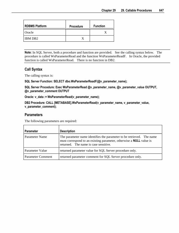
Chapter 29 29. Callable Procedures 647
RDBMS Platform Procedure Function
Oracle X
IBM DB2 X
Note: In SQL Server, both a procedure and function are provided. See the calling syntax below. The
procedure is called WsParameterRead and the function WsParameterReadF. In Oracle, the provided
function is called WsParameterRead. There is no function in DB2.
Call Syntax
The calling syntax is:
SQL Server Function: SELECT dbo.WsParameterReadF(@v_parameter_name);
SQL Server Procedure: Exec WsParameterRead @v_parameter_name, @v_parameter_value OUTPUT, @v_parameter_comment OUTPUT
Oracle: v_data := WsParameterRead(v_parameter_name);
DB2 Procedure: CALL [METABASE].WsParameterRead(v_parameter_name, v_parameter_value, v_parameter_comment);
Parameters
The following parameters are required:
Parameter Description
Parameter Name The parameter name identifies the parameter to be retrieved. The name
must correspond to an existing parameter, otherwise a NULL value is
returned. The name is case sensitive.
Parameter Value returned parameter value for SQL Server procedure only.
Parameter Comment returned parameter comment for SQL Server procedure only.
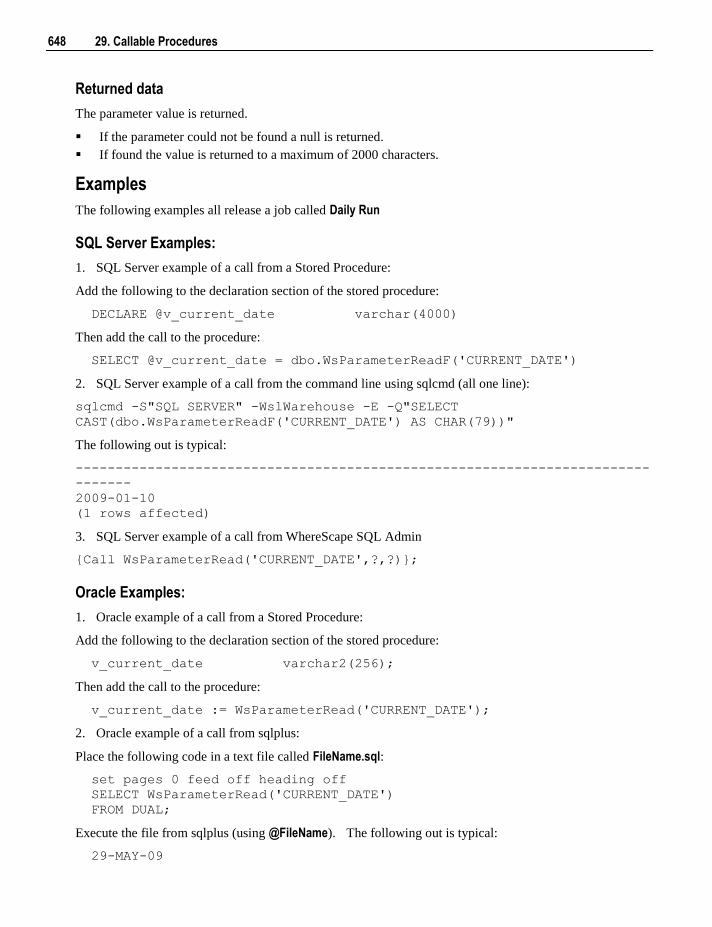
648 29. Callable Procedures
Returned data
The parameter value is returned.
If the parameter could not be found a null is returned.
If found the value is returned to a maximum of 2000 characters.
Examples
The following examples all release a job called Daily Run
SQL Server Examples:
1. SQL Server example of a call from a Stored Procedure:
Add the following to the declaration section of the stored procedure:
DECLARE @v_current_date varchar(4000)
Then add the call to the procedure:
SELECT @v_current_date = dbo.WsParameterReadF('CURRENT_DATE')
2. SQL Server example of a call from the command line using sqlcmd (all one line):
sqlcmd -S"SQL SERVER" -WslWarehouse -E -Q"SELECT
CAST(dbo.WsParameterReadF('CURRENT_DATE') AS CHAR(79))"
The following out is typical:
------------------------------------------------------------------------
-------
2009-01-10
(1 rows affected)
3. SQL Server example of a call from WhereScape SQL Admin
{Call WsParameterRead('CURRENT_DATE',?,?)};
Oracle Examples:
1. Oracle example of a call from a Stored Procedure:
Add the following to the declaration section of the stored procedure:
v_current_date varchar2(256);
Then add the call to the procedure:
v_current_date := WsParameterRead('CURRENT_DATE');
2. Oracle example of a call from sqlplus:
Place the following code in a text file called FileName.sql:
set pages 0 feed off heading off
SELECT WsParameterRead('CURRENT_DATE')
FROM DUAL;
Execute the file from sqlplus (using @FileName). The following out is typical:
29-MAY-09
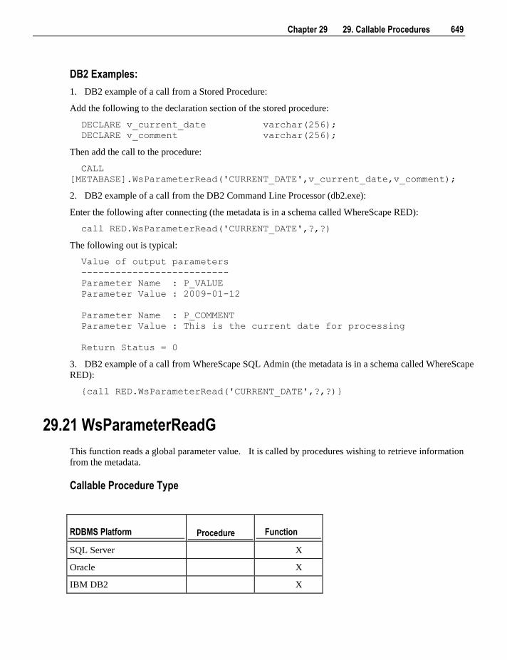
Chapter 29 29. Callable Procedures 649
DB2 Examples:
1. DB2 example of a call from a Stored Procedure:
Add the following to the declaration section of the stored procedure:
DECLARE v_current_date varchar(256);
DECLARE v_comment varchar(256);
Then add the call to the procedure:
CALL
[METABASE].WsParameterRead('CURRENT_DATE',v_current_date,v_comment);
2. DB2 example of a call from the DB2 Command Line Processor (db2.exe):
Enter the following after connecting (the metadata is in a schema called WhereScape RED):
call RED.WsParameterRead('CURRENT_DATE',?,?)
The following out is typical:
Value of output parameters
--------------------------
Parameter Name : P_VALUE
Parameter Value : 2009-01-12
Parameter Name : P_COMMENT
Parameter Value : This is the current date for processing
Return Status = 0
3. DB2 example of a call from WhereScape SQL Admin (the metadata is in a schema called WhereScape
RED):
{call RED.WsParameterRead('CURRENT_DATE',?,?)}
29.21 WsParameterReadG
This function reads a global parameter value. It is called by procedures wishing to retrieve information
from the metadata.
Callable Procedure Type
RDBMS Platform Procedure Function
SQL Server X
Oracle X
IBM DB2 X
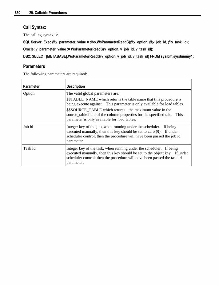
650 29. Callable Procedures
Call Syntax:
The calling syntax is:
SQL Server: Exec @v_parameter_value = dbo.WsParameterReadG(@v_option, @v_job_id, @v_task_id);
Oracle: v_parameter_value := WsParameterReadG(v_option, v_job_id, v_task_id);
DB2: SELECT [METABASE].WsParameterReadG(v_option, v_job_id, v_task_id) FROM sysibm.sysdummy1;
Parameters
The following parameters are required:
Parameter Description
Option The valid global parameters are:
$$TABLE_NAME which returns the table name that this procedure is
being execute against. This parameter is only available for load tables.
$$SOURCE_TABLE which returns the maximum value in the
source_table field of the column properties for the specified tale. This
parameter is only available for load tables.
Job id Integer key of the job, when running under the scheduler. If being
executed manually, then this key should be set to zero (0). If under
scheduler control, then the procedure will have been passed the job id
parameter.
Task Id Integer key of the task, when running under the scheduler. If being
executed manually, then this key should be set to the object key. If under
scheduler control, then the procedure will have been passed the task id
parameter.
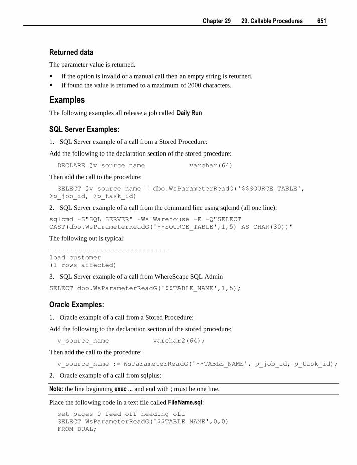
Chapter 29 29. Callable Procedures 651
Returned data
The parameter value is returned.
If the option is invalid or a manual call then an empty string is returned.
If found the value is returned to a maximum of 2000 characters.
Examples
The following examples all release a job called Daily Run
SQL Server Examples:
1. SQL Server example of a call from a Stored Procedure:
Add the following to the declaration section of the stored procedure:
DECLARE @v_source_name varchar(64)
Then add the call to the procedure:
SELECT @v_source_name = dbo.WsParameterReadG('$$SOURCE_TABLE',
@p_job_id, @p_task_id)
2. SQL Server example of a call from the command line using sqlcmd (all one line):
sqlcmd -S"SQL SERVER" -WslWarehouse -E -Q"SELECT
CAST(dbo.WsParameterReadG('$$SOURCE_TABLE',1,5) AS CHAR(30))"
The following out is typical:
------------------------------
load_customer
(1 rows affected)
3. SQL Server example of a call from WhereScape SQL Admin
SELECT dbo.WsParameterReadG('$$TABLE_NAME',1,5);
Oracle Examples:
1. Oracle example of a call from a Stored Procedure:
Add the following to the declaration section of the stored procedure:
v_source_name varchar2(64);
Then add the call to the procedure:
v_source_name := WsParameterReadG('$$TABLE_NAME', p_job_id, p_task_id);
2. Oracle example of a call from sqlplus:
Note: the line beginning exec ... and end with ; must be one line.
Place the following code in a text file called FileName.sql:
set pages 0 feed off heading off
SELECT WsParameterReadG('$$TABLE_NAME',0,0)
FROM DUAL;
652 29. Callable Procedures
Execute the file from sqlplus (using @FileName). The following out is typical:
load_customer
DB2 Examples:
1. DB2 example of a call from a Stored Procedure:
Add the following to the declaration section of the stored procedure:
DECLARE v_table_name VARCHAR(256);
Then add the call to the procedure:
CALL [METABASE].WsParameterReadG('$$TABLE_NAME', p_job_id, p_task_id,
v_table_name);
2. DB2 example of a call from the DB2 Command Line Processor (db2.exe):
Enter the following after connecting (the metadata is in a schema called WhereScape RED):
call RED.WsParameterReadG('$$TABLE_NAME',0,0,?)
The following out is typical:
Value of output parameters
--------------------------
Parameter Name : P_VALUE
Parameter Value : load_customer
Return Status = 0
3. DB2 example of a call from WhereScape SQL Admin (the metadata is in a schema called WhereScape
RED):
{Call RED.WsParameterReadG('$$TABLE_NAME',0,0,?)}
29.22 WsParameterReadJ
This function reads job information and attributes. It is called by procedures wishing to retrieve
information stored against the job that is executing them.
Callable Procedure Type
RDBMS Platform Procedure Function
SQL Server X
Oracle X
IBM DB2 X
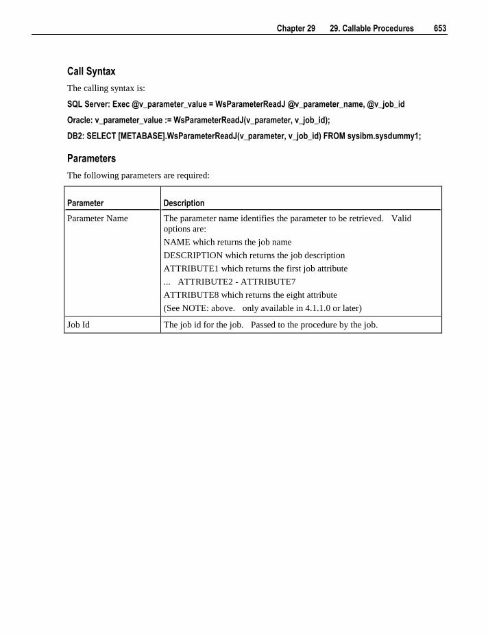
Chapter 29 29. Callable Procedures 653
Call Syntax
The calling syntax is:
SQL Server: Exec @v_parameter_value = WsParameterReadJ @v_parameter_name, @v_job_id
Oracle: v_parameter_value := WsParameterReadJ(v_parameter, v_job_id);
DB2: SELECT [METABASE].WsParameterReadJ(v_parameter, v_job_id) FROM sysibm.sysdummy1;
Parameters
The following parameters are required:
Parameter Description
Parameter Name The parameter name identifies the parameter to be retrieved. Valid
options are:
NAME which returns the job name
DESCRIPTION which returns the job description
ATTRIBUTE1 which returns the first job attribute
... ATTRIBUTE2 - ATTRIBUTE7
ATTRIBUTE8 which returns the eight attribute
(See NOTE: above. only available in 4.1.1.0 or later)
Job Id The job id for the job. Passed to the procedure by the job.
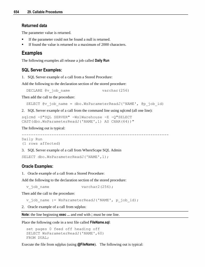
654 29. Callable Procedures
Returned data
The parameter value is returned.
If the parameter could not be found a null is returned.
If found the value is returned to a maximum of 2000 characters.
Examples
The following examples all release a job called Daily Run
SQL Server Examples:
1. SQL Server example of a call from a Stored Procedure:
Add the following to the declaration section of the stored procedure:
DECLARE @v_job_name varchar(256)
Then add the call to the procedure:
SELECT @v_job_name = dbo.WsParameterReadJ('NAME', @p_job_id)
2. SQL Server example of a call from the command line using sqlcmd (all one line):
sqlcmd -S"SQL SERVER" -WslWarehouse -E -Q"SELECT
CAST(dbo.WsParameterReadJ('NAME',1) AS CHAR(64))"
The following out is typical:
----------------------------------------------------------------
Daily Run
(1 rows affected)
3. SQL Server example of a call from WhereScape SQL Admin
SELECT dbo.WsParameterReadJ('NAME',1);
Oracle Examples:
1. Oracle example of a call from a Stored Procedure:
Add the following to the declaration section of the stored procedure:
v_job_name varchar2(256);
Then add the call to the procedure:
v_job_name := WsParameterReadJ('NAME', p_job_id);
2. Oracle example of a call from sqlplus:
Note: the line beginning exec ... and end with ; must be one line.
Place the following code in a text file called FileName.sql:
set pages 0 feed off heading off
SELECT WsParameterReadJ('NAME',60)
FROM DUAL;
Execute the file from sqlplus (using @FileName). The following out is typical:
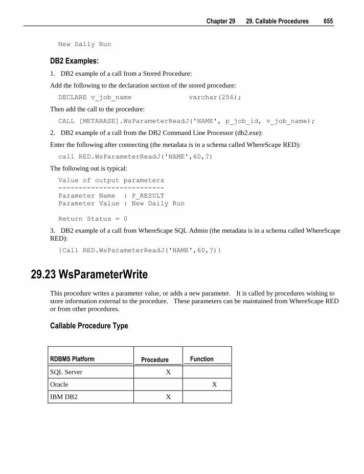
Chapter 29 29. Callable Procedures 655
New Daily Run
DB2 Examples:
1. DB2 example of a call from a Stored Procedure:
Add the following to the declaration section of the stored procedure:
DECLARE v_job_name varchar(256);
Then add the call to the procedure:
CALL [METABASE].WsParameterReadJ('NAME', p_job_id, v_job_name);
2. DB2 example of a call from the DB2 Command Line Processor (db2.exe):
Enter the following after connecting (the metadata is in a schema called WhereScape RED):
call RED.WsParameterReadJ('NAME',60,?)
The following out is typical:
Value of output parameters
--------------------------
Parameter Name : P_RESULT
Parameter Value : New Daily Run
Return Status = 0
3. DB2 example of a call from WhereScape SQL Admin (the metadata is in a schema called WhereScape
RED):
{Call RED.WsParameterReadJ('NAME',60,?)}
29.23 WsParameterWrite
This procedure writes a parameter value, or adds a new parameter. It is called by procedures wishing to
store information external to the procedure. These parameters can be maintained from WhereScape RED
or from other procedures.
Callable Procedure Type
RDBMS Platform Procedure Function
SQL Server X
Oracle X
IBM DB2 X
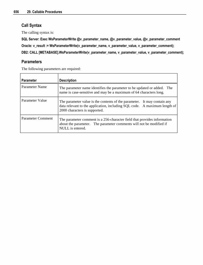
656 29. Callable Procedures
Call Syntax
The calling syntax is:
SQL Server: Exec WsParameterWrite @v_parameter_name, @v_parameter_value, @v_parameter_comment
Oracle: v_result := WsParameterWrite(v_parameter_name, v_parameter_value, v_parameter_comment);
DB2: CALL [METABASE].WsParameterWrite(v_parameter_name, v_parameter_value, v_parameter_comment);
Parameters
The following parameters are required:
Parameter Description
Parameter Name The parameter name identifies the parameter to be updated or added. The
name is case-sensitive and may be a maximum of 64 characters long.
Parameter Value The parameter value is the contents of the parameter. It may contain any
data relevant to the application, including SQL code. A maximum length of
2000 characters is supported.
Parameter Comment The parameter comment is a 256-character field that provides information
about the parameter. The parameter comments will not be modified if
NULL is entered.
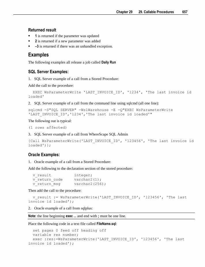
Chapter 29 29. Callable Procedures 657
Returned result
1 is returned if the parameter was updated
2 is returned if a new parameter was added
–3 is returned if there was an unhandled exception.
Examples
The following examples all release a job called Daily Run
SQL Server Examples:
1. SQL Server example of a call from a Stored Procedure:
Add the call to the procedure:
EXEC WsParameterWrite 'LAST_INVOICE_ID', '1234', 'The last invoice id
loaded'
2. SQL Server example of a call from the command line using sqlcmd (all one line):
sqlcmd -S"SQL SERVER" -WslWarehouse -E -Q"EXEC WsParameterWrite
'LAST_INVOICE_ID','1234','The last invoice id loaded'"
The following out is typical:
(1 rows affected)
3. SQL Server example of a call from WhereScape SQL Admin
{Call WsParameterWrite('LAST_INVOICE_ID', '123456', 'The last invoice id
loaded')};
Oracle Examples:
1. Oracle example of a call from a Stored Procedure:
Add the following to the declaration section of the stored procedure:
v_result integer;
v_return_code varchar2(1);
v_return_msg varchar2(256);
Then add the call to the procedure:
v_result := WsParameterWrite('LAST_INVOICE_ID', '123456', 'The last
invoice id loaded');
2. Oracle example of a call from sqlplus:
Note: the line beginning exec ... and end with ; must be one line.
Place the following code in a text file called FileName.sql:
set pages 0 feed off heading off
variable res number;
exec :res:=WsParameterWrite('LAST_INVOICE_ID', '123456', 'The last
invoice id loaded');
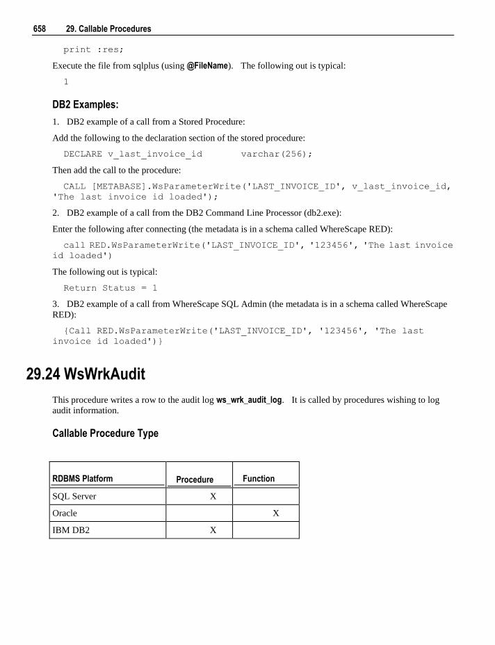
658 29. Callable Procedures
print :res;
Execute the file from sqlplus (using @FileName). The following out is typical:
1
DB2 Examples:
1. DB2 example of a call from a Stored Procedure:
Add the following to the declaration section of the stored procedure:
DECLARE v_last_invoice_id varchar(256);
Then add the call to the procedure:
CALL [METABASE].WsParameterWrite('LAST_INVOICE_ID', v_last_invoice_id,
'The last invoice id loaded');
2. DB2 example of a call from the DB2 Command Line Processor (db2.exe):
Enter the following after connecting (the metadata is in a schema called WhereScape RED):
call RED.WsParameterWrite('LAST_INVOICE_ID', '123456', 'The last invoice
id loaded')
The following out is typical:
Return Status = 1
3. DB2 example of a call from WhereScape SQL Admin (the metadata is in a schema called WhereScape
RED):
{Call RED.WsParameterWrite('LAST_INVOICE_ID', '123456', 'The last
invoice id loaded')}
29.24 WsWrkAudit
This procedure writes a row to the audit log ws_wrk_audit_log. It is called by procedures wishing to log
audit information.
Callable Procedure Type
RDBMS Platform Procedure Function
SQL Server X
Oracle X
IBM DB2 X
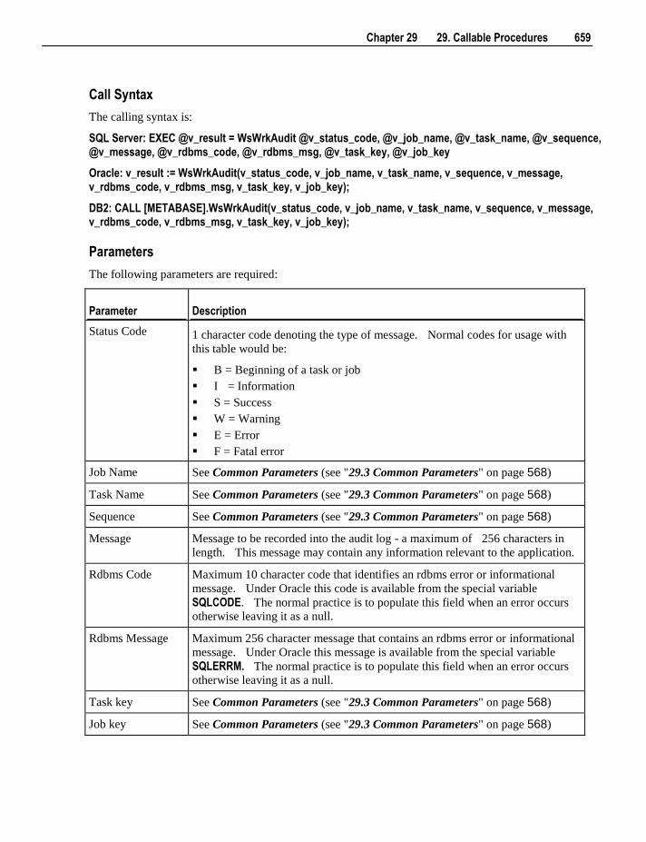
Chapter 29 29. Callable Procedures 659
Call Syntax
The calling syntax is:
SQL Server: EXEC @v_result = WsWrkAudit @v_status_code, @v_job_name, @v_task_name, @v_sequence, @v_message, @v_rdbms_code, @v_rdbms_msg, @v_task_key, @v_job_key
Oracle: v_result := WsWrkAudit(v_status_code, v_job_name, v_task_name, v_sequence, v_message, v_rdbms_code, v_rdbms_msg, v_task_key, v_job_key);
DB2: CALL [METABASE].WsWrkAudit(v_status_code, v_job_name, v_task_name, v_sequence, v_message, v_rdbms_code, v_rdbms_msg, v_task_key, v_job_key);
Parameters
The following parameters are required:
Parameter Description
Status Code 1 character code denoting the type of message. Normal codes for usage with
this table would be:
B = Beginning of a task or job
I = Information
S = Success
W = Warning
E = Error
F = Fatal error
Job Name See Common Parameters (see "29.3 Common Parameters" on page 568)
Task Name See Common Parameters (see "29.3 Common Parameters" on page 568)
Sequence See Common Parameters (see "29.3 Common Parameters" on page 568)
Message Message to be recorded into the audit log - a maximum of 256 characters in
length. This message may contain any information relevant to the application.
Rdbms Code Maximum 10 character code that identifies an rdbms error or informational
message. Under Oracle this code is available from the special variable
SQLCODE. The normal practice is to populate this field when an error occurs
otherwise leaving it as a null.
Rdbms Message Maximum 256 character message that contains an rdbms error or informational
message. Under Oracle this message is available from the special variable
SQLERRM. The normal practice is to populate this field when an error occurs
otherwise leaving it as a null.
Task key See Common Parameters (see "29.3 Common Parameters" on page 568)
Job key See Common Parameters (see "29.3 Common Parameters" on page 568)
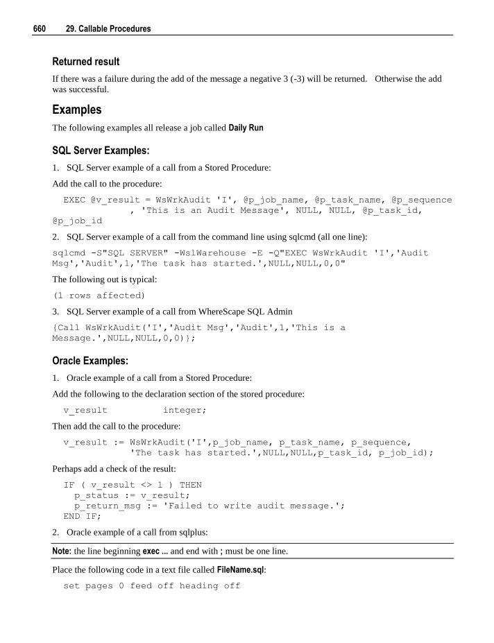
660 29. Callable Procedures
Returned result
If there was a failure during the add of the message a negative 3 (-3) will be returned. Otherwise the add
was successful.
Examples
The following examples all release a job called Daily Run
SQL Server Examples:
1. SQL Server example of a call from a Stored Procedure:
Add the call to the procedure:
EXEC @v_result = WsWrkAudit 'I', @p_job_name, @p_task_name, @p_sequence
, 'This is an Audit Message', NULL, NULL, @p_task_id,
@p_job_id
2. SQL Server example of a call from the command line using sqlcmd (all one line):
sqlcmd -S"SQL SERVER" -WslWarehouse -E -Q"EXEC WsWrkAudit 'I','Audit
Msg','Audit',1,'The task has started.',NULL,NULL,0,0"
The following out is typical:
(1 rows affected)
3. SQL Server example of a call from WhereScape SQL Admin
{Call WsWrkAudit('I','Audit Msg','Audit',1,'This is a
Message.',NULL,NULL,0,0)};
Oracle Examples:
1. Oracle example of a call from a Stored Procedure:
Add the following to the declaration section of the stored procedure:
v_result integer;
Then add the call to the procedure:
v_result := WsWrkAudit('I',p_job_name, p_task_name, p_sequence,
'The task has started.',NULL,NULL,p_task_id, p_job_id);
Perhaps add a check of the result:
IF ( v_result <> 1 ) THEN
p_status := v_result;
p_return_msg := 'Failed to write audit message.';
END IF;
2. Oracle example of a call from sqlplus:
Note: the line beginning exec ... and end with ; must be one line.
Place the following code in a text file called FileName.sql:
set pages 0 feed off heading off
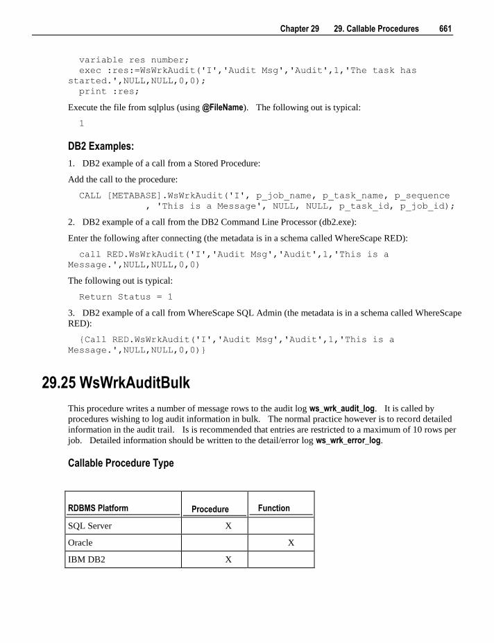
Chapter 29 29. Callable Procedures 661
variable res number;
exec :res:=WsWrkAudit('I','Audit Msg','Audit',1,'The task has
started.',NULL,NULL,0,0);
print :res;
Execute the file from sqlplus (using @FileName). The following out is typical:
1
DB2 Examples:
1. DB2 example of a call from a Stored Procedure:
Add the call to the procedure:
CALL [METABASE].WsWrkAudit('I', p_job_name, p_task_name, p_sequence
, 'This is a Message', NULL, NULL, p_task_id, p_job_id);
2. DB2 example of a call from the DB2 Command Line Processor (db2.exe):
Enter the following after connecting (the metadata is in a schema called WhereScape RED):
call RED.WsWrkAudit('I','Audit Msg','Audit',1,'This is a
Message.',NULL,NULL,0,0)
The following out is typical:
Return Status = 1
3. DB2 example of a call from WhereScape SQL Admin (the metadata is in a schema called WhereScape
RED):
{Call RED.WsWrkAudit('I','Audit Msg','Audit',1,'This is a
Message.',NULL,NULL,0,0)}
29.25 WsWrkAuditBulk
This procedure writes a number of message rows to the audit log ws_wrk_audit_log. It is called by
procedures wishing to log audit information in bulk. The normal practice however is to record detailed
information in the audit trail. Is is recommended that entries are restricted to a maximum of 10 rows per
job. Detailed information should be written to the detail/error log ws_wrk_error_log.
Callable Procedure Type
RDBMS Platform Procedure Function
SQL Server X
Oracle X
IBM DB2 X
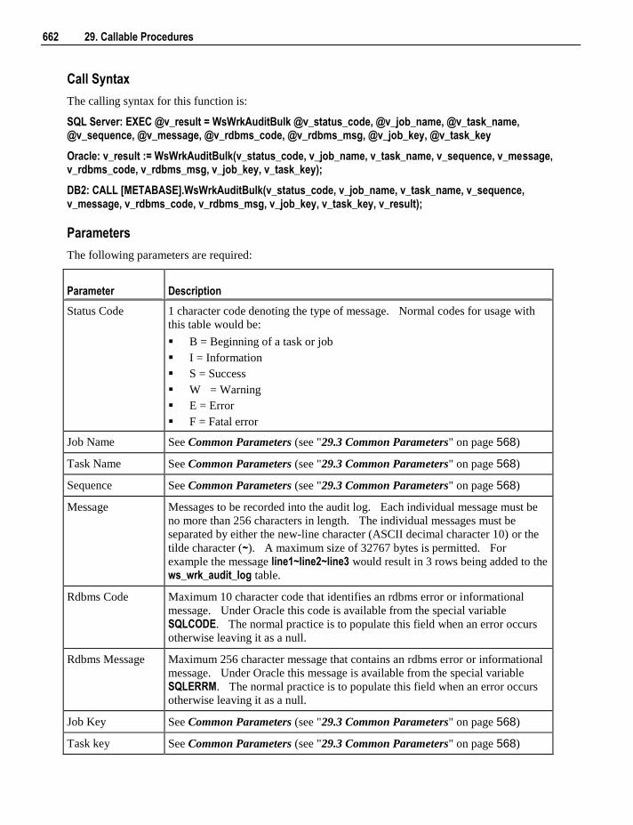
662 29. Callable Procedures
Call Syntax
The calling syntax for this function is:
SQL Server: EXEC @v_result = WsWrkAuditBulk @v_status_code, @v_job_name, @v_task_name, @v_sequence, @v_message, @v_rdbms_code, @v_rdbms_msg, @v_job_key, @v_task_key
Oracle: v_result := WsWrkAuditBulk(v_status_code, v_job_name, v_task_name, v_sequence, v_message, v_rdbms_code, v_rdbms_msg, v_job_key, v_task_key);
DB2: CALL [METABASE].WsWrkAuditBulk(v_status_code, v_job_name, v_task_name, v_sequence, v_message, v_rdbms_code, v_rdbms_msg, v_job_key, v_task_key, v_result);
Parameters
The following parameters are required:
Parameter Description
Status Code 1 character code denoting the type of message. Normal codes for usage with
this table would be:
B = Beginning of a task or job
I = Information
S = Success
W = Warning
E = Error
F = Fatal error
Job Name See Common Parameters (see "29.3 Common Parameters" on page 568)
Task Name See Common Parameters (see "29.3 Common Parameters" on page 568)
Sequence See Common Parameters (see "29.3 Common Parameters" on page 568)
Message Messages to be recorded into the audit log. Each individual message must be
no more than 256 characters in length. The individual messages must be
separated by either the new-line character (ASCII decimal character 10) or the
tilde character (~). A maximum size of 32767 bytes is permitted. For
example the message line1~line2~line3 would result in 3 rows being added to the
ws_wrk_audit_log table.
Rdbms Code Maximum 10 character code that identifies an rdbms error or informational
message. Under Oracle this code is available from the special variable
SQLCODE. The normal practice is to populate this field when an error occurs
otherwise leaving it as a null.
Rdbms Message Maximum 256 character message that contains an rdbms error or informational
message. Under Oracle this message is available from the special variable
SQLERRM. The normal practice is to populate this field when an error occurs
otherwise leaving it as a null.
Job Key See Common Parameters (see "29.3 Common Parameters" on page 568)
Task key See Common Parameters (see "29.3 Common Parameters" on page 568)

Chapter 29 29. Callable Procedures 663
Parameter Description
Result Integer that indicates the status of the call to this procedure. See below for the
possible values of Result. DB2 only.
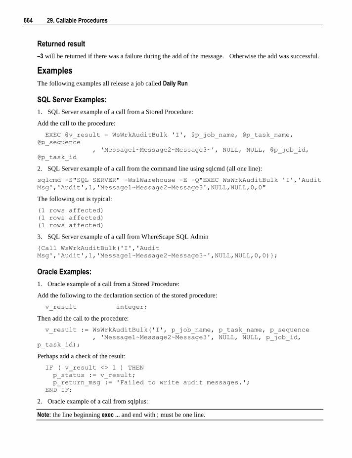
664 29. Callable Procedures
Returned result
–3 will be returned if there was a failure during the add of the message. Otherwise the add was successful.
Examples
The following examples all release a job called Daily Run
SQL Server Examples:
1. SQL Server example of a call from a Stored Procedure:
Add the call to the procedure:
EXEC @v_result = WsWrkAuditBulk 'I', @p_job_name, @p_task_name,
@p_sequence
, 'Message1~Message2~Message3~', NULL, NULL, @p_job_id,
@p_task_id
2. SQL Server example of a call from the command line using sqlcmd (all one line):
sqlcmd -S"SQL SERVER" -WslWarehouse -E -Q"EXEC WsWrkAuditBulk 'I','Audit
Msg','Audit',1,'Message1~Message2~Message3',NULL,NULL,0,0"
The following out is typical:
(1 rows affected)
(1 rows affected)
(1 rows affected)
3. SQL Server example of a call from WhereScape SQL Admin
{Call WsWrkAuditBulk('I','Audit
Msg','Audit',1,'Message1~Message2~Message3~',NULL,NULL,0,0)};
Oracle Examples:
1. Oracle example of a call from a Stored Procedure:
Add the following to the declaration section of the stored procedure:
v_result integer;
Then add the call to the procedure:
v_result := WsWrkAuditBulk('I', p_job_name, p_task_name, p_sequence
, 'Message1~Message2~Message3', NULL, NULL, p_job_id,
p_task_id);
Perhaps add a check of the result:
IF ( v_result <> 1 ) THEN
p_status := v_result;
p_return_msg := 'Failed to write audit messages.';
END IF;
2. Oracle example of a call from sqlplus:
Note: the line beginning exec ... and end with ; must be one line.
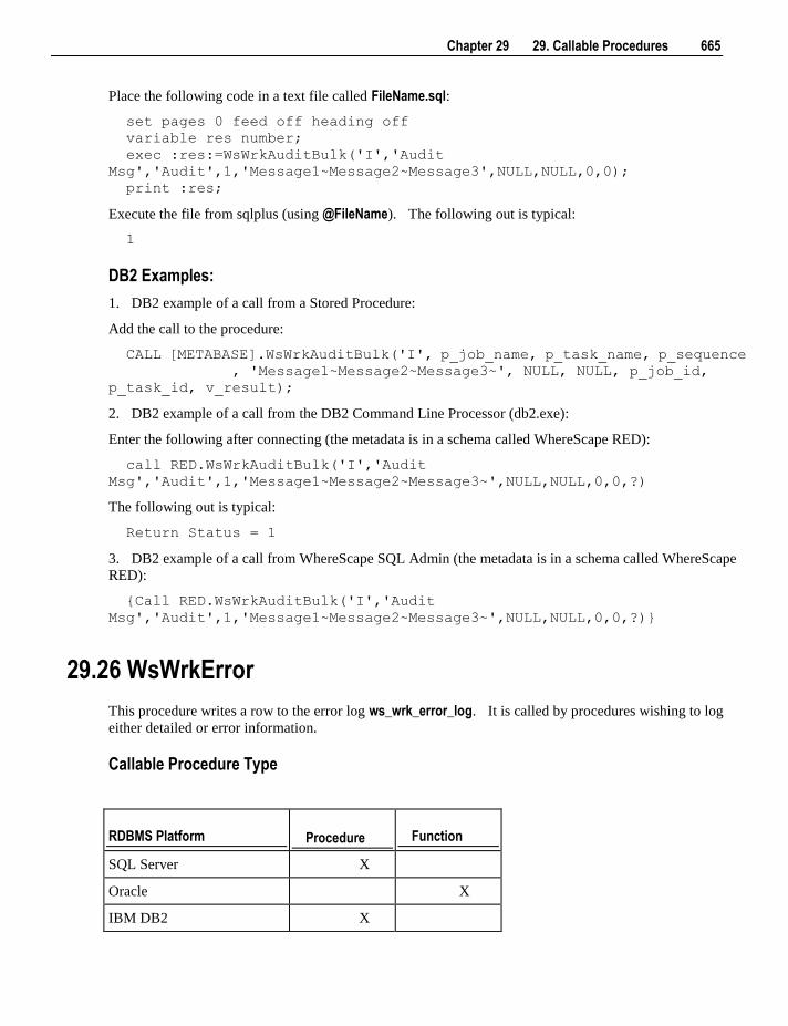
Chapter 29 29. Callable Procedures 665
Place the following code in a text file called FileName.sql:
set pages 0 feed off heading off
variable res number;
exec :res:=WsWrkAuditBulk('I','Audit
Msg','Audit',1,'Message1~Message2~Message3',NULL,NULL,0,0);
print :res;
Execute the file from sqlplus (using @FileName). The following out is typical:
1
DB2 Examples:
1. DB2 example of a call from a Stored Procedure:
Add the call to the procedure:
CALL [METABASE].WsWrkAuditBulk('I', p_job_name, p_task_name, p_sequence
, 'Message1~Message2~Message3~', NULL, NULL, p_job_id,
p_task_id, v_result);
2. DB2 example of a call from the DB2 Command Line Processor (db2.exe):
Enter the following after connecting (the metadata is in a schema called WhereScape RED):
call RED.WsWrkAuditBulk('I','Audit
Msg','Audit',1,'Message1~Message2~Message3~',NULL,NULL,0,0,?)
The following out is typical:
Return Status = 1
3. DB2 example of a call from WhereScape SQL Admin (the metadata is in a schema called WhereScape
RED):
{Call RED.WsWrkAuditBulk('I','Audit
Msg','Audit',1,'Message1~Message2~Message3~',NULL,NULL,0,0,?)}
29.26 WsWrkError
This procedure writes a row to the error log ws_wrk_error_log. It is called by procedures wishing to log
either detailed or error information.
Callable Procedure Type
RDBMS Platform Procedure Function
SQL Server X
Oracle X
IBM DB2 X
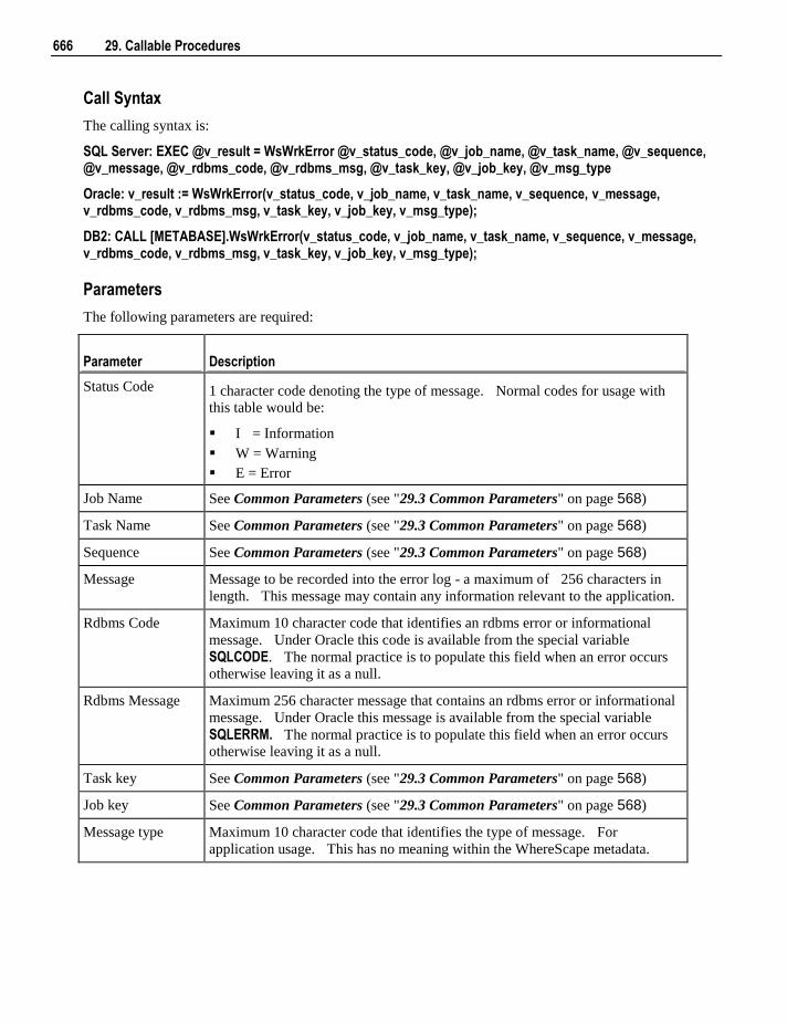
666 29. Callable Procedures
Call Syntax
The calling syntax is:
SQL Server: EXEC @v_result = WsWrkError @v_status_code, @v_job_name, @v_task_name, @v_sequence, @v_message, @v_rdbms_code, @v_rdbms_msg, @v_task_key, @v_job_key, @v_msg_type
Oracle: v_result := WsWrkError(v_status_code, v_job_name, v_task_name, v_sequence, v_message, v_rdbms_code, v_rdbms_msg, v_task_key, v_job_key, v_msg_type);
DB2: CALL [METABASE].WsWrkError(v_status_code, v_job_name, v_task_name, v_sequence, v_message, v_rdbms_code, v_rdbms_msg, v_task_key, v_job_key, v_msg_type);
Parameters
The following parameters are required:
Parameter Description
Status Code 1 character code denoting the type of message. Normal codes for usage with
this table would be:
I = Information
W = Warning
E = Error
Job Name See Common Parameters (see "29.3 Common Parameters" on page 568)
Task Name See Common Parameters (see "29.3 Common Parameters" on page 568)
Sequence See Common Parameters (see "29.3 Common Parameters" on page 568)
Message Message to be recorded into the error log - a maximum of 256 characters in
length. This message may contain any information relevant to the application.
Rdbms Code Maximum 10 character code that identifies an rdbms error or informational
message. Under Oracle this code is available from the special variable
SQLCODE. The normal practice is to populate this field when an error occurs
otherwise leaving it as a null.
Rdbms Message Maximum 256 character message that contains an rdbms error or informational
message. Under Oracle this message is available from the special variable
SQLERRM. The normal practice is to populate this field when an error occurs
otherwise leaving it as a null.
Task key See Common Parameters (see "29.3 Common Parameters" on page 568)
Job key See Common Parameters (see "29.3 Common Parameters" on page 568)
Message type Maximum 10 character code that identifies the type of message. For
application usage. This has no meaning within the WhereScape metadata.
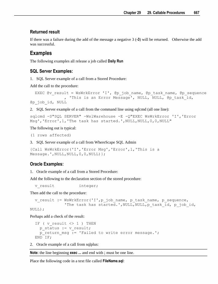
Chapter 29 29. Callable Procedures 667
Returned result
If there was a failure during the add of the message a negative 3 (-3) will be returned. Otherwise the add
was successful.
Examples
The following examples all release a job called Daily Run
SQL Server Examples:
1. SQL Server example of a call from a Stored Procedure:
Add the call to the procedure:
EXEC @v_result = WsWrkError 'I', @p_job_name, @p_task_name, @p_sequence
, 'This is an Error Message', NULL, NULL, @p_task_id,
@p_job_id, NULL
2. SQL Server example of a call from the command line using sqlcmd (all one line):
sqlcmd -S"SQL SERVER" -WslWarehouse -E -Q"EXEC WsWrkError 'I','Error
Msg','Error',1,'The task has started.',NULL,NULL,0,0,NULL"
The following out is typical:
(1 rows affected)
3. SQL Server example of a call from WhereScape SQL Admin
{Call WsWrkError('I','Error Msg','Error',1,'This is a
Message.',NULL,NULL,0,0,NULL)};
Oracle Examples:
1. Oracle example of a call from a Stored Procedure:
Add the following to the declaration section of the stored procedure:
v_result integer;
Then add the call to the procedure:
v_result := WsWrkError('I',p_job_name, p_task_name, p_sequence,
'The task has started.',NULL,NULL,p_task_id, p_job_id,
NULL);
Perhaps add a check of the result:
IF ( v_result <> 1 ) THEN
p_status := v_result;
p_return_msg := 'Failed to write error message.';
END IF;
2. Oracle example of a call from sqlplus:
Note: the line beginning exec ... and end with ; must be one line.
Place the following code in a text file called FileName.sql:
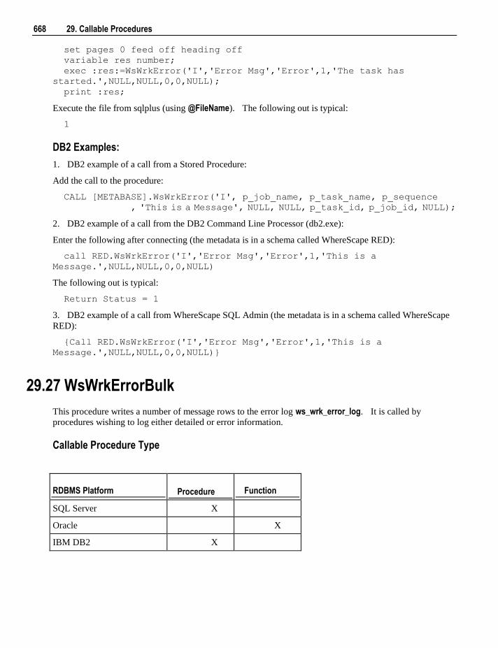
668 29. Callable Procedures
set pages 0 feed off heading off
variable res number;
exec :res:=WsWrkError('I','Error Msg','Error',1,'The task has
started.',NULL,NULL,0,0,NULL);
print :res;
Execute the file from sqlplus (using @FileName). The following out is typical:
1
DB2 Examples:
1. DB2 example of a call from a Stored Procedure:
Add the call to the procedure:
CALL [METABASE].WsWrkError('I', p_job_name, p_task_name, p_sequence
, 'This is a Message', NULL, NULL, p_task_id, p_job_id, NULL);
2. DB2 example of a call from the DB2 Command Line Processor (db2.exe):
Enter the following after connecting (the metadata is in a schema called WhereScape RED):
call RED.WsWrkError('I','Error Msg','Error',1,'This is a
Message.',NULL,NULL,0,0,NULL)
The following out is typical:
Return Status = 1
3. DB2 example of a call from WhereScape SQL Admin (the metadata is in a schema called WhereScape
RED):
{Call RED.WsWrkError('I','Error Msg','Error',1,'This is a
Message.',NULL,NULL,0,0,NULL)}
29.27 WsWrkErrorBulk
This procedure writes a number of message rows to the error log ws_wrk_error_log. It is called by
procedures wishing to log either detailed or error information.
Callable Procedure Type
RDBMS Platform Procedure Function
SQL Server X
Oracle X
IBM DB2 X
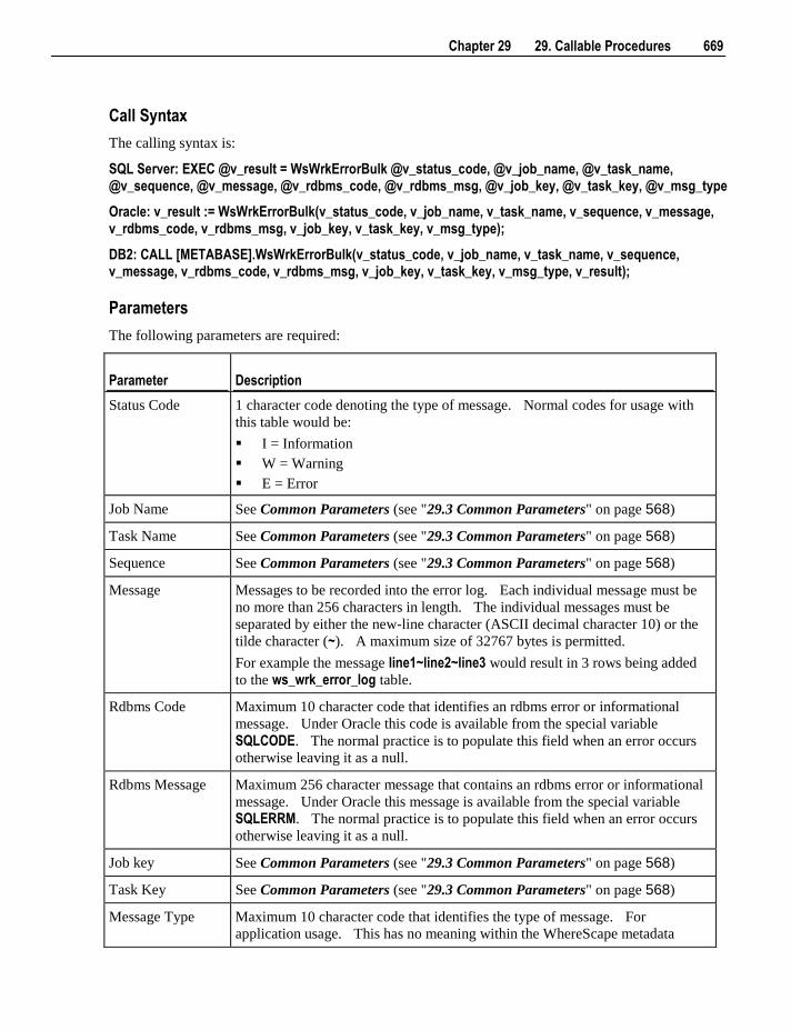
Chapter 29 29. Callable Procedures 669
Call Syntax
The calling syntax is:
SQL Server: EXEC @v_result = WsWrkErrorBulk @v_status_code, @v_job_name, @v_task_name, @v_sequence, @v_message, @v_rdbms_code, @v_rdbms_msg, @v_job_key, @v_task_key, @v_msg_type
Oracle: v_result := WsWrkErrorBulk(v_status_code, v_job_name, v_task_name, v_sequence, v_message, v_rdbms_code, v_rdbms_msg, v_job_key, v_task_key, v_msg_type);
DB2: CALL [METABASE].WsWrkErrorBulk(v_status_code, v_job_name, v_task_name, v_sequence, v_message, v_rdbms_code, v_rdbms_msg, v_job_key, v_task_key, v_msg_type, v_result);
Parameters
The following parameters are required:
Parameter Description
Status Code 1 character code denoting the type of message. Normal codes for usage with
this table would be:
I = Information
W = Warning
E = Error
Job Name See Common Parameters (see "29.3 Common Parameters" on page 568)
Task Name See Common Parameters (see "29.3 Common Parameters" on page 568)
Sequence See Common Parameters (see "29.3 Common Parameters" on page 568)
Message Messages to be recorded into the error log. Each individual message must be
no more than 256 characters in length. The individual messages must be
separated by either the new-line character (ASCII decimal character 10) or the
tilde character (~). A maximum size of 32767 bytes is permitted.
For example the message line1~line2~line3 would result in 3 rows being added
to the ws_wrk_error_log table.
Rdbms Code Maximum 10 character code that identifies an rdbms error or informational
message. Under Oracle this code is available from the special variable
SQLCODE. The normal practice is to populate this field when an error occurs
otherwise leaving it as a null.
Rdbms Message Maximum 256 character message that contains an rdbms error or informational
message. Under Oracle this message is available from the special variable
SQLERRM. The normal practice is to populate this field when an error occurs
otherwise leaving it as a null.
Job key See Common Parameters (see "29.3 Common Parameters" on page 568)
Task Key See Common Parameters (see "29.3 Common Parameters" on page 568)
Message Type Maximum 10 character code that identifies the type of message. For
application usage. This has no meaning within the WhereScape metadata
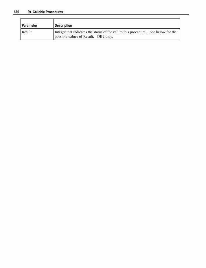
670 29. Callable Procedures
Parameter Description
Result Integer that indicates the status of the call to this procedure. See below for the
possible values of Result. DB2 only.
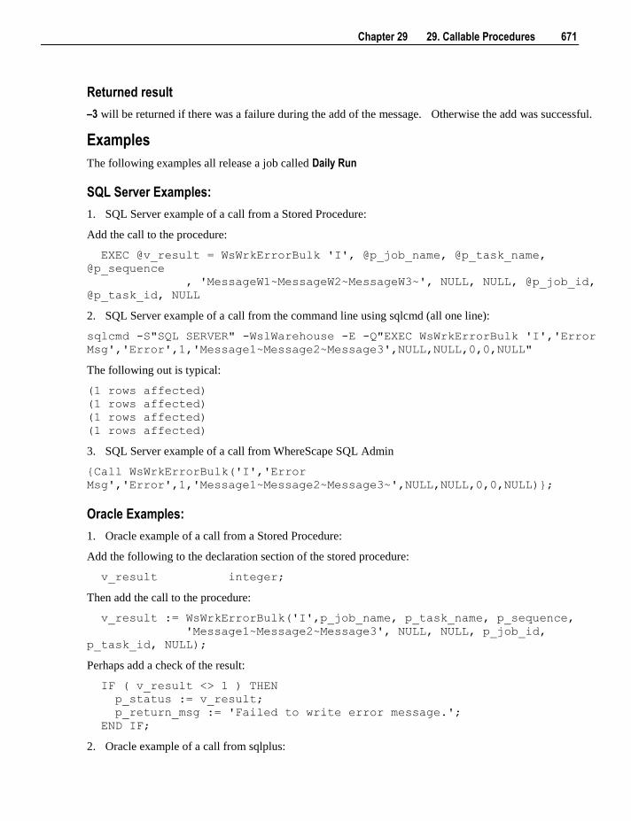
Chapter 29 29. Callable Procedures 671
Returned result
–3 will be returned if there was a failure during the add of the message. Otherwise the add was successful.
Examples
The following examples all release a job called Daily Run
SQL Server Examples:
1. SQL Server example of a call from a Stored Procedure:
Add the call to the procedure:
EXEC @v_result = WsWrkErrorBulk 'I', @p_job_name, @p_task_name,
@p_sequence
, 'MessageW1~MessageW2~MessageW3~', NULL, NULL, @p_job_id,
@p_task_id, NULL
2. SQL Server example of a call from the command line using sqlcmd (all one line):
sqlcmd -S"SQL SERVER" -WslWarehouse -E -Q"EXEC WsWrkErrorBulk 'I','Error
Msg','Error',1,'Message1~Message2~Message3',NULL,NULL,0,0,NULL"
The following out is typical:
(1 rows affected)
(1 rows affected)
(1 rows affected)
(1 rows affected)
3. SQL Server example of a call from WhereScape SQL Admin
{Call WsWrkErrorBulk('I','Error
Msg','Error',1,'Message1~Message2~Message3~',NULL,NULL,0,0,NULL)};
Oracle Examples:
1. Oracle example of a call from a Stored Procedure:
Add the following to the declaration section of the stored procedure:
v_result integer;
Then add the call to the procedure:
v_result := WsWrkErrorBulk('I',p_job_name, p_task_name, p_sequence,
'Message1~Message2~Message3', NULL, NULL, p_job_id,
p_task_id, NULL);
Perhaps add a check of the result:
IF ( v_result <> 1 ) THEN
p_status := v_result;
p_return_msg := 'Failed to write error message.';
END IF;
2. Oracle example of a call from sqlplus:
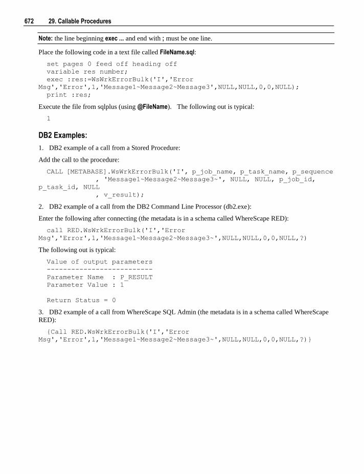
672 29. Callable Procedures
Note: the line beginning exec ... and end with ; must be one line.
Place the following code in a text file called FileName.sql:
set pages 0 feed off heading off
variable res number;
exec :res:=WsWrkErrorBulk('I','Error
Msg','Error',1,'Message1~Message2~Message3',NULL,NULL,0,0,NULL);
print :res;
Execute the file from sqlplus (using @FileName). The following out is typical:
1
DB2 Examples:
1. DB2 example of a call from a Stored Procedure:
Add the call to the procedure:
CALL [METABASE].WsWrkErrorBulk('I', p_job_name, p_task_name, p_sequence
, 'Message1~Message2~Message3~', NULL, NULL, p_job_id,
p_task_id, NULL
, v_result);
2. DB2 example of a call from the DB2 Command Line Processor (db2.exe):
Enter the following after connecting (the metadata is in a schema called WhereScape RED):
call RED.WsWrkErrorBulk('I','Error
Msg','Error',1,'Message1~Message2~Message3~',NULL,NULL,0,0,NULL,?)
The following out is typical:
Value of output parameters
--------------------------
Parameter Name : P_RESULT
Parameter Value : 1
Return Status = 0
3. DB2 example of a call from WhereScape SQL Admin (the metadata is in a schema called WhereScape
RED):
{Call RED.WsWrkErrorBulk('I','Error
Msg','Error',1,'Message1~Message2~Message3~',NULL,NULL,0,0,NULL,?)}
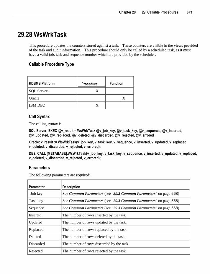
Chapter 29 29. Callable Procedures 673
29.28 WsWrkTask
This procedure updates the counters stored against a task. These counters are visible in the views provided
of the task and audit information. This procedure should only be called by a scheduled task, as it must
have a valid job, task and sequence number which are provided by the scheduler.
Callable Procedure Type
RDBMS Platform Procedure Function
SQL Server X
Oracle X
IBM DB2 X
Call Syntax
The calling syntax is:
SQL Server: EXEC @v_result = WsWrkTask @v_job_key, @v_task_key, @v_sequence, @v_inserted, @v_updated, @v_replaced, @v_deleted, @v_discarded, @v_rejected, @v_errored
Oracle: v_result := WsWrkTask(v_job_key, v_task_key, v_sequence, v_inserted, v_updated, v_replaced, v_deleted, v_discarded, v_rejected, v_errored);
DB2: CALL [METABASE].WsWrkTask(v_job_key, v_task_key, v_sequence, v_inserted, v_updated, v_replaced, v_deleted, v_discarded, v_rejected, v_errored);
Parameters
The following parameters are required:
Parameter Description
Job key See Common Parameters (see "29.3 Common Parameters" on page 568)
Task key See Common Parameters (see "29.3 Common Parameters" on page 568)
Sequence See Common Parameters (see "29.3 Common Parameters" on page 568)
Inserted The number of rows inserted by the task.
Updated The number of rows updated by the task.
Replaced The number of rows replaced by the task.
Deleted The number of rows deleted by the task.
Discarded The number of rows discarded by the task.
Rejected The number of rows rejected by the task.
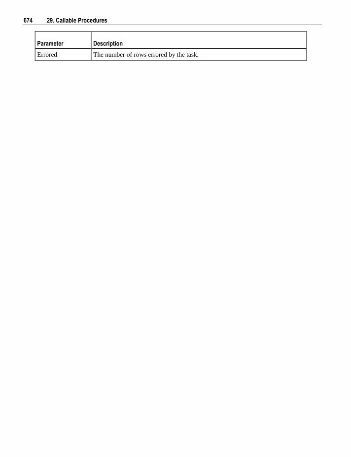
674 29. Callable Procedures
Parameter Description
Errored The number of rows errored by the task.
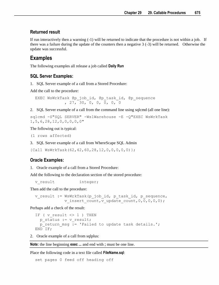
Chapter 29 29. Callable Procedures 675
Returned result
If run interactively then a warning (-1) will be returned to indicate that the procedure is not within a job. If
there was a failure during the update of the counters then a negative 3 (-3) will be returned. Otherwise the
update was successful.
Examples
The following examples all release a job called Daily Run
SQL Server Examples:
1. SQL Server example of a call from a Stored Procedure:
Add the call to the procedure:
EXEC WsWrkTask @p_job_id, @p_task_id, @p_sequence
, 27, 30, 0, 0, 0, 0, 0
2. SQL Server example of a call from the command line using sqlcmd (all one line):
sqlcmd -S"SQL SERVER" -WslWarehouse -E -Q"EXEC WsWrkTask
1,5,6,28,12,0,0,0,0,0"
The following out is typical:
(1 rows affected)
3. SQL Server example of a call from WhereScape SQL Admin
{Call WsWrkTask(62,42,60,28,12,0,0,0,0,0)};
Oracle Examples:
1. Oracle example of a call from a Stored Procedure:
Add the following to the declaration section of the stored procedure:
v_result integer;
Then add the call to the procedure:
v_result := WsWrkTask(p_job_id, p_task_id, p_sequence,
v_insert_count,v_update_count,0,0,0,0,0);
Perhaps add a check of the result:
IF ( v_result <> 1 ) THEN
p_status := v_result;
p_return_msg := 'Failed to update task details.';
END IF;
2. Oracle example of a call from sqlplus:
Note: the line beginning exec ... and end with ; must be one line.
Place the following code in a text file called FileName.sql:
set pages 0 feed off heading off
676 29. Callable Procedures
variable res number;
exec :res:=WsWrkTask(62,42,60,28,12,0,0,0,0,0);
print :res;
Execute the file from sqlplus (using @FileName). The following out is typical:
1
DB2 Examples:
1. DB2 example of a call from a Stored Procedure:
Add the call to the procedure:
CALL [METABASE].WsWrkTask(p_job_id, p_task_id, p_sequence
, 27, 30, 0, 0, 0, 0, 0);
2. DB2 example of a call from the DB2 Command Line Processor (db2.exe):
Enter the following after connecting (the metadata is in a schema called WhereScape RED):
call RED.WsWrkTask(62,42,60,28,12,0,0,0,0,0)
The following out is typical:
Return Status = 0
3. DB2 example of a call from WhereScape SQL Admin (the metadata is in a schema called WhereScape
RED):
{Call RED.WsWrkTask(62,42,60,28,12,0,0,0,0,0)}
Chapter 30 30. Retrofitting 677
WhereScape RED includes an advanced retrofit capability that can be used to:
1 Migrate an existing data warehouse from one relational database to another (known as fork-lifting).
2 Load a data model from a modelling tool.
Retrofitting is achieved using the Retro Copy object type in WhereScape RED and the Retrofit tables wizard.
Retrofitting (see "30. Retrofitting" on page 675, "16.8 Retrofitting an OLAP Object" on page 370)
In This Chapter
30.1 Migrating the Data Warehouse Database Platform ............. 675
30.2 Importing a Data Model ...................................................... 680
30.3 Re-Target Source Tables ..................................................... 684
30.4 Retro Copy Column Properties ........................................... 686
30.1 Migrating the Data Warehouse Database Platform
WhereScape RED has an advanced retrofitting wizard for migrating an existing data warehouse from one
relational database to another.
The steps to use this wizard are:
1 Create a connection object for the old data warehouse database, populating the following fields:
Connection Name
Connection Type => ODBC
ODBC Source
Work Directory
Extract user name
Extract password
Note: The extract user must be able to select from all tables to be migrated.
2 Ensure all naming standards in Tools / Options are set to match the objects being retrofitted. This
saves work later.
3 Right click on the Retro Copy object group in the object tree in the left pane and choose Select source tables:
C H A P T E R 3 0
30. Retrofitting
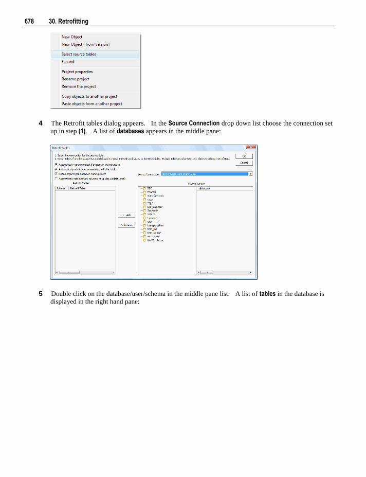
678 30. Retrofitting
4 The Retrofit tables dialog appears. In the Source Connection drop down list choose the connection set
up in step (1). A list of databases appears in the middle pane:
5 Double click on the database/user/schema in the middle pane list. A list of tables in the database is
displayed in the right hand pane:
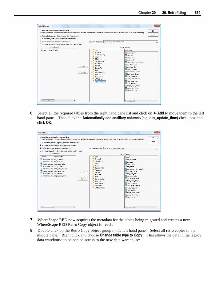
Chapter 30 30. Retrofitting 679
6 Select all the required tables from the right hand pane list and click on <- Add to move them to the left
hand pane. Then click the Automatically add ancillary columns (e.g. dss_update_time) check box and
click OK.
7 WhereScape RED now acquires the metadata for the tables being migrated and creates a new
WhereScape RED Retro Copy object for each.
8 Double click on the Retro Copy object group in the left hand pane. Select all retro copies in the
middle pane. Right click and choose Change table type to Copy. This allows the data in the legacy
data warehouse to be copied across to the new data warehouse:
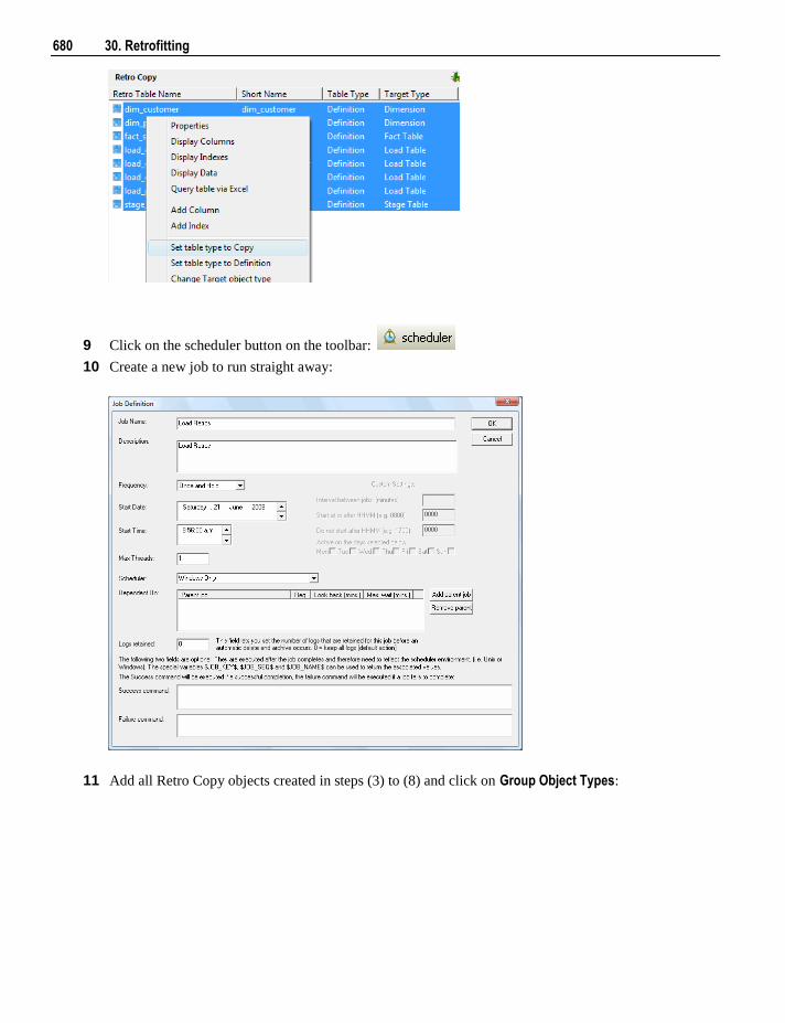
680 30. Retrofitting
9 Click on the scheduler button on the toolbar:
10 Create a new job to run straight away:
11 Add all Retro Copy objects created in steps (3) to (8) and click on Group Object Types:
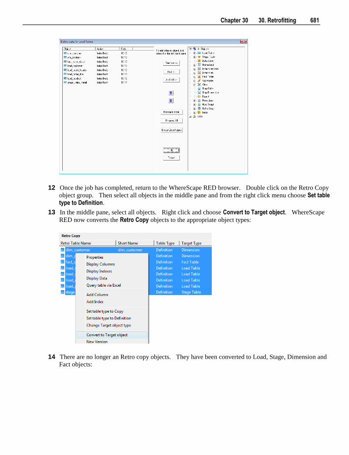
Chapter 30 30. Retrofitting 681
12 Once the job has completed, return to the WhereScape RED browser. Double click on the Retro Copy
object group. Then select all objects in the middle pane and from the right click menu choose Set table type to Definition.
13 In the middle pane, select all objects. Right click and choose Convert to Target object. WhereScape
RED now converts the Retro Copy objects to the appropriate object types:
14 There are no longer an Retro copy objects. They have been converted to Load, Stage, Dimension and
Fact objects:
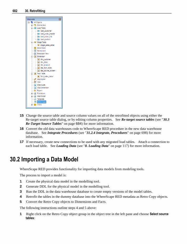
682 30. Retrofitting
15 Change the source table and source column values on all of the retrofitted objects using either the
Re-target source table dialog, or by editing column properties. See Re-target source tables (see "30.3
Re-Target Source Tables" on page 684) for more information.
16 Convert the old data warehouses code to WhereScape RED procedure in the new data warehouse
database. See Integrate Procedures (see "31.2.4 Integrate, Procedures" on page 698) for more
information.
17 If necessary, create new connections to be used with any migrated load tables. Attach a connection to
each load table. See Loading Data (see "8. Loading Data" on page 117) for more information.
30.2 Importing a Data Model
WhereScape RED provides functionality for importing data models from modeling tools.
The process to import a model is:
1 Create the physical data model in the modelling tool.
2 Generate DDL for the physical model in the modelling tool.
3 Run the DDL in the data warehouse database to create empty versions of the model tables.
4 Retrofit the tables in the dummy database into the WhereScape RED metadata as Retro Copy objects.
5 Convert the Retro Copy objects to Dimensions and Facts.
The following instructions outline steps 4 and 5 above:
1 Right click on the Retro Copy object group in the object tree in the left pane and choose Select source tables:
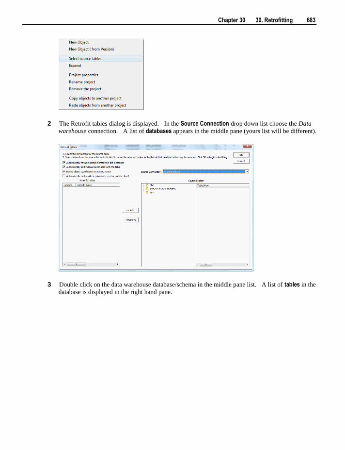
Chapter 30 30. Retrofitting 683
2 The Retrofit tables dialog is displayed. In the Source Connection drop down list choose the Data
warehouse connection. A list of databases appears in the middle pane (yours list will be different).
3 Double click on the data warehouse database/schema in the middle pane list. A list of tables in the
database is displayed in the right hand pane.
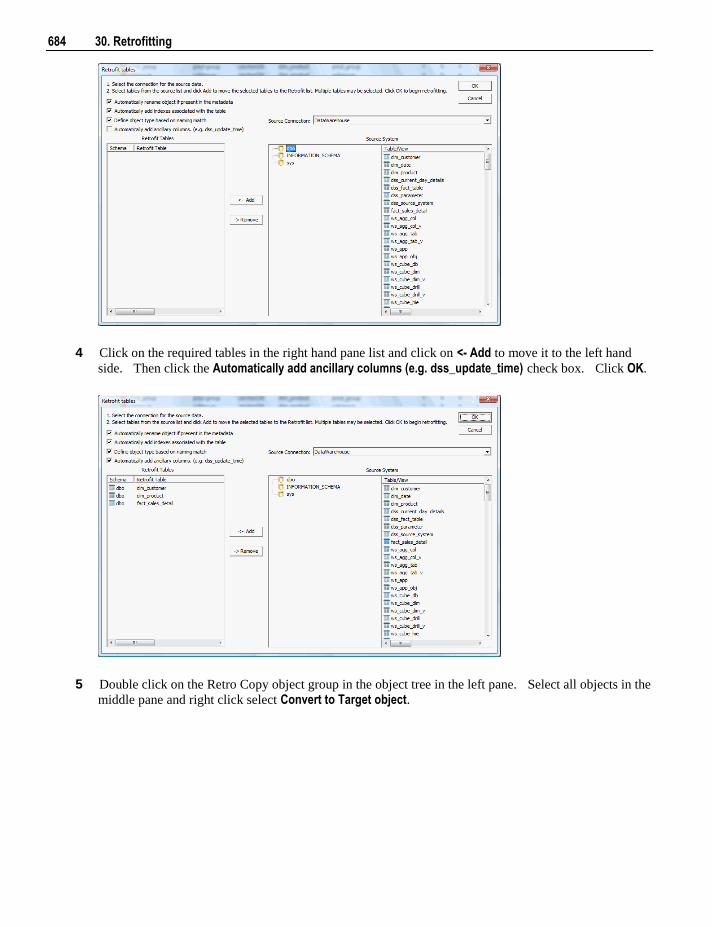
684 30. Retrofitting
4 Click on the required tables in the right hand pane list and click on <- Add to move it to the left hand
side. Then click the Automatically add ancillary columns (e.g. dss_update_time) check box. Click OK.
5 Double click on the Retro Copy object group in the object tree in the left pane. Select all objects in the
middle pane and right click select Convert to Target object.
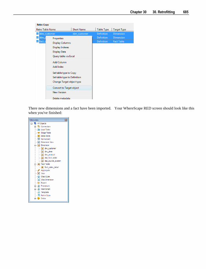
Chapter 30 30. Retrofitting 685
There new dimensions and a fact have been imported. Your WhereScape RED screen should look like this
when you've finished:
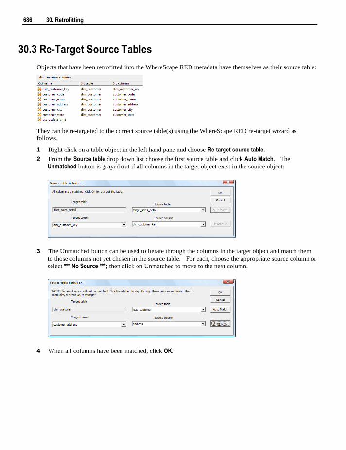
686 30. Retrofitting
30.3 Re-Target Source Tables
Objects that have been retrofitted into the WhereScape RED metadata have themselves as their source table:
They can be re-targeted to the correct source table(s) using the WhereScape RED re-target wizard as
follows.
1 Right click on a table object in the left hand pane and choose Re-target source table.
2 From the Source table drop down list choose the first source table and click Auto Match. The
Unmatched button is grayed out if all columns in the target object exist in the source object:
3 The Unmatched button can be used to iterate through the columns in the target object and match them
to those columns not yet chosen in the source table. For each, choose the appropriate source column or
select *** No Source ***; then click on Unmatched to move to the next column.
4 When all columns have been matched, click OK.
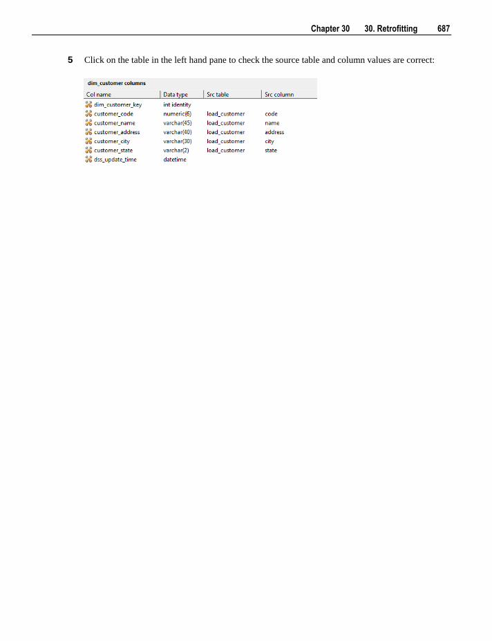
Chapter 30 30. Retrofitting 687
5 Click on the table in the left hand pane to check the source table and column values are correct:
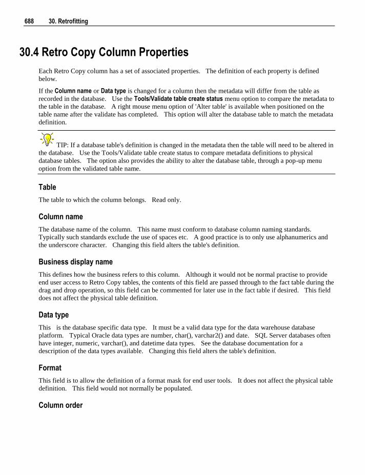
688 30. Retrofitting
30.4 Retro Copy Column Properties
Each Retro Copy column has a set of associated properties. The definition of each property is defined
below.
If the Column name or Data type is changed for a column then the metadata will differ from the table as
recorded in the database. Use the Tools/Validate table create status menu option to compare the metadata to
the table in the database. A right mouse menu option of 'Alter table' is available when positioned on the
table name after the validate has completed. This option will alter the database table to match the metadata
definition.
TIP: If a database table's definition is changed in the metadata then the table will need to be altered in
the database. Use the Tools/Validate table create status to compare metadata definitions to physical
database tables. The option also provides the ability to alter the database table, through a pop-up menu
option from the validated table name.
Table
The table to which the column belongs. Read only.
Column name
The database name of the column. This name must conform to database column naming standards.
Typically such standards exclude the use of spaces etc. A good practice is to only use alphanumerics and
the underscore character. Changing this field alters the table's definition.
Business display name
This defines how the business refers to this column. Although it would not be normal practise to provide
end user access to Retro Copy tables, the contents of this field are passed through to the fact table during the
drag and drop operation, so this field can be commented for later use in the fact table if desired. This field
does not affect the physical table definition.
Data type
This is the database specific data type. It must be a valid data type for the data warehouse database
platform. Typical Oracle data types are number, char(), varchar2() and date. SQL Server databases often
have integer, numeric, varchar(), and datetime data types. See the database documentation for a
description of the data types available. Changing this field alters the table's definition.
Format
This field is to allow the definition of a format mask for end user tools. It does not affect the physical table
definition. This field would not normally be populated.
Column order
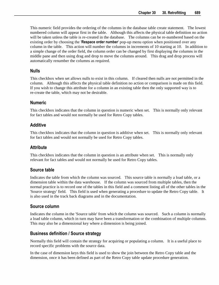
Chapter 30 30. Retrofitting 689
This numeric field provides the ordering of the columns in the database table create statement. The lowest
numbered column will appear first in the table. Although this affects the physical table definition no action
will be taken unless the table is re-created in the database. The columns can be re-numbered based on the
existing order by choosing the 'Respace order number' pop-up menu option when positioned over any
column in the table. This action will number the columns in increments of 10 starting at 10. In addition to
a simple change of the order field, the column order can be changed by first displaying the columns in the
middle pane and then using drag and drop to move the columns around. This drag and drop process will
automatically renumber the columns as required.
Nulls
This checkbox when set allows nulls to exist in this column. If cleared then nulls are not permitted in the
column. Although this affects the physical table definition no action or comparison is made on this field.
If you wish to change this attribute for a column in an existing table then the only supported way is to
re-create the table, which may not be desirable.
Numeric
This checkbox indicates that the column in question is numeric when set. This is normally only relevant
for fact tables and would not normally be used for Retro Copy tables.
Additive
This checkbox indicates that the column in question is additive when set. This is normally only relevant
for fact tables and would not normally be used for Retro Copy tables.
Attribute
This checkbox indicates that the column in question is an attribute when set. This is normally only
relevant for fact tables and would not normally be used for Retro Copy tables.
Source table
Indicates the table from which the column was sourced. This source table is normally a load table, or a
dimension table within the data warehouse. If the column was sourced from multiple tables, then the
normal practice is to record one of the tables in this field and a comment listing all of the other tables in the
'Source strategy' field. This field is used when generating a procedure to update the Retro Copy table. It
is also used in the track back diagrams and in the documentation.
Source column
Indicates the column in the 'Source table' from which the column was sourced. Such a column is normally
a load table column, which in turn may have been a transformation or the combination of multiple columns.
This may also be a dimensional key where a dimension is being joined.
Business definition / Source strategy
Normally this field will contain the strategy for acquiring or populating a column. It is a useful place to
record specific problems with the source data.
In the case of dimension keys this field is used to show the join between the Retro Copy table and the
dimension, once it has been defined as part of the Retro Copy table update procedure generation.
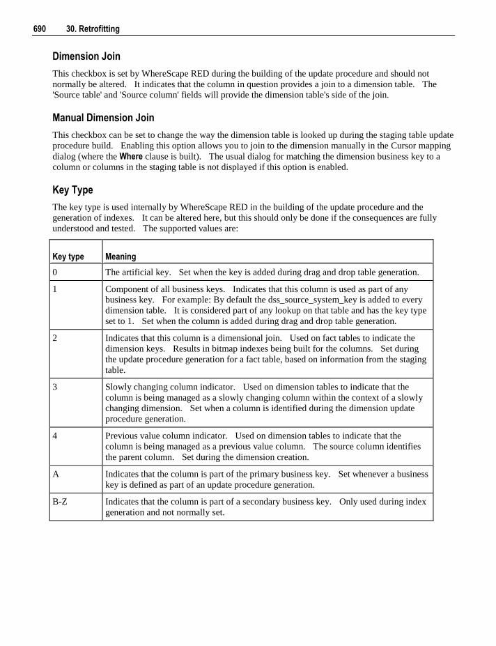
690 30. Retrofitting
Dimension Join
This checkbox is set by WhereScape RED during the building of the update procedure and should not
normally be altered. It indicates that the column in question provides a join to a dimension table. The
'Source table' and 'Source column' fields will provide the dimension table's side of the join.
Manual Dimension Join
This checkbox can be set to change the way the dimension table is looked up during the staging table update
procedure build. Enabling this option allows you to join to the dimension manually in the Cursor mapping
dialog (where the Where clause is built). The usual dialog for matching the dimension business key to a
column or columns in the staging table is not displayed if this option is enabled.
Key Type
The key type is used internally by WhereScape RED in the building of the update procedure and the
generation of indexes. It can be altered here, but this should only be done if the consequences are fully
understood and tested. The supported values are:
Key type Meaning
0 The artificial key. Set when the key is added during drag and drop table generation.
1 Component of all business keys. Indicates that this column is used as part of any
business key. For example: By default the dss_source_system_key is added to every
dimension table. It is considered part of any lookup on that table and has the key type
set to 1. Set when the column is added during drag and drop table generation.
2 Indicates that this column is a dimensional join. Used on fact tables to indicate the
dimension keys. Results in bitmap indexes being built for the columns. Set during
the update procedure generation for a fact table, based on information from the staging
table.
3 Slowly changing column indicator. Used on dimension tables to indicate that the
column is being managed as a slowly changing column within the context of a slowly
changing dimension. Set when a column is identified during the dimension update
procedure generation.
4 Previous value column indicator. Used on dimension tables to indicate that the
column is being managed as a previous value column. The source column identifies
the parent column. Set during the dimension creation.
A Indicates that the column is part of the primary business key. Set whenever a business
key is defined as part of an update procedure generation.
B-Z Indicates that the column is part of a secondary business key. Only used during index
generation and not normally set.
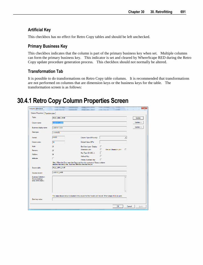
Chapter 30 30. Retrofitting 691
Artificial Key
This checkbox has no effect for Retro Copy tables and should be left unchecked.
Primary Business Key
This checkbox indicates that the column is part of the primary business key when set. Multiple columns
can form the primary business key. This indicator is set and cleared by WhereScape RED during the Retro
Copy update procedure generation process. This checkbox should not normally be altered.
Transformation Tab
It is possible to do transformations on Retro Copy table columns. It is recommended that transformations
are not performed on columns that are dimension keys or the business keys for the table. The
transformation screen is as follows:
30.4.1 Retro Copy Column Properties Screen

Chapter 31 31. Integrating WhereScape RED into an Existing Warehouse 693
Two main options exist in terms of bringing WhereScape RED into an existing data warehouse
environment:
1 Rebuild tables and procedures with WhereScape RED.
2 Integrating existing tables and procedures into WhereScape RED.
Both options require manual coding changes to stored procedures. The main advantages and disadvantages
of these two options are discusses below, and in detail in the following sections.
Rebuilding
The rebuild option is essentially a redevelopment of the existing data warehouse utilizing the knowledge
acquired in the initial development and the rapid development capabilities of WhereScape RED. A rebuild
will take more time and effort than just integrating existing tables and procedures but will provide a better
platform on which to extend the data warehouse. See the Rebuild (see "31.1 Rebuild" on page 692)
section for the approach to achieve this option.
Integrate
Existing data warehouse tables can be identified to WhereScape RED. The tables are seen and can be
managed to a degree. The main disadvantage is the increased difficulty in utilizing these tables when
trying to extend the data warehouse. This option is however significantly quicker and easier than a rebuild.
It is discussed in detail in the Integrate (see "31.2 Integrate" on page 692) section of this chapter.
The decision as to which option to choose will depend on the size and complexity of the existing data
warehouse. Another important factor is the degree to which the existing data warehouse is to be extended.
If future enhancements revolve around new analysis areas that have little overlap with the existing
environment then a integrate may be the best answer. If the data warehouse is small and relatively simple
than a rebuild may be worth considering. In any event the best plan may be to do a test integrate and then
re-evaluate the situation.
In This Chapter
31.1 Rebuild ................................................................................ 692
31.2 Integrate .............................................................................. 692
C H A P T E R 3 1
31. Integrating WhereScape RED into an Existing Warehouse
694 31. Integrating WhereScape RED into an Existing Warehouse
31.1 Rebuild
The rebuild process essentially is a total re-creation of the data warehouse. One of the major impacts of
such an approach is the 'end user layer', or rather the effect on the end user tools and saved queries and
reports that are currently in use. The redesign or redeployment of this interface to the end users of the data
warehouse may be too large a task to undertake. The problem can be circumvented to some degree though
the use of views to make the new data warehouse environment look the same as the previous. But it is this
impact and the subsequent re-testing process that must be considered when deciding to undertake a rebuild.
The advantages of a rebuild is the seamless integration of future analysis areas into the data warehouse and
the single point of management that is provided. The major steps in the rebuild process will depend very
much on the environment being replaced. As a guideline the following steps may be worth considering.
The rebuild process
1 Load a copy of the WhereScape metadata repository into an otherwise empty test environment. See
the Installation and Administration Guide for instructions on how to load a metadata repository.
2 Ensure there are no public synonyms that point to existing table names, if the rebuild process is to use
the same names as some or all of the existing tables.
Working within the WhereScape RED tool proceed to:
3 Create connections to the new test data warehouse and to all the source systems.
4 Using the source system knowledge from the existing data warehouse, create the appropriate load
tables in the data warehouse based on the existing extract or load methodology.
5 Build up the dimension, stage and fact tables using the same column and table names where possible.
6 Examine the existing procedures or update methodology and include this into the generated stored
procedures.
7 Test the new environment.
8 Work out a plan to convert the existing data into the new data warehouse. Where possible it is best to
keep existing key values and re-assign sequences to match these existing key values where appropriate.
9 Convert and test the old data warehouse data in the new environment.
10 Redeploy the end user tool access.
31.2 Integrate
The integrate process
The steps in the integrate process are:
1 Create a test environment (database user) with the existing data warehouse tables loaded.
2 Load a copy of the WhereScape metadata repository into this test environment. See the Installation
and Administration Guide for instructions on how to load a metadata repository.
Working within the WhereScape RED tool proceed to:
3 Create any connections to Unix or Windows servers where host scripts are currently executed. See
either creating a Windows connection (see "6.6 Connections to Windows" on page 99) or creating a
Unix connection (see "6.5 Connections to Unix" on page 95).
Chapter 31 31. Integrating WhereScape RED into an Existing Warehouse 695
4 Create a Data Warehouse connection mapping back to the test environment. See creating a
connection to the data warehouse (see "6.2 Connection to the Data Warehouse" on page 78).
5 Incorporate any Host system scripts currently used. See incorporating host scripts (see "31.2.1
Integrate, Host Scripts" on page 693).
6 Browse the Data Warehouse connection (Browse/Source Tables).
7 Drag and drop each existing data warehouse table into an appropriate object type. See Selecting an
appropriate table type (see "31.2.2 Integrate, Selecting a Table Type" on page 694)
8 Answer the retrofit questions, and build any required procedures. See integrate questions (see "31.2.3
Integrate, Questions" on page 695).
9 Edit and amend all generated procedures, or create new procedures to handle the existing processing
methodology. See procedure changes (see "31.2.4 Integrate, Procedures" on page 698).
10 Test the new environment.
Removing the metadata for a table
It is possible to delete the metadata for a table without deleting the table itself. For example if the integrate
process is incorrectly undertaken, the metadata for the specific table can be removed. To delete the
metadata only: First select the table and using the right mouse menu select 'Delete'. A dialog box will ask
if you wish to delete the object and drop the table. Answer NO. A second dialog box will now appear
asking if just the metadata is to be deleted. Answer Yes to this question and only the metadata will be
removed.
31.2.1 Integrate, Host Scripts Existing host scripts (either Unix or Windows) can be brought into the WhereScape RED metadata. To
incorporate an existing script the process is as follows:
1 Create a 'Host Script' object using WhereScape RED. In the left hand pane click on a project or the
'All Objects' project and using the right mouse menu select 'Create Object'. The new object dialog box
will appear. From the Object Type drop down select 'Host Script' and enter a name for the new
script.
2 The following properties dialog will appear. Select the script type. Either Unix or Windows script.
Select the appropriate connection from the 'Default Connect' drop down. Fill in the purpose field to
define the role of the script and then click Update to store the changes.
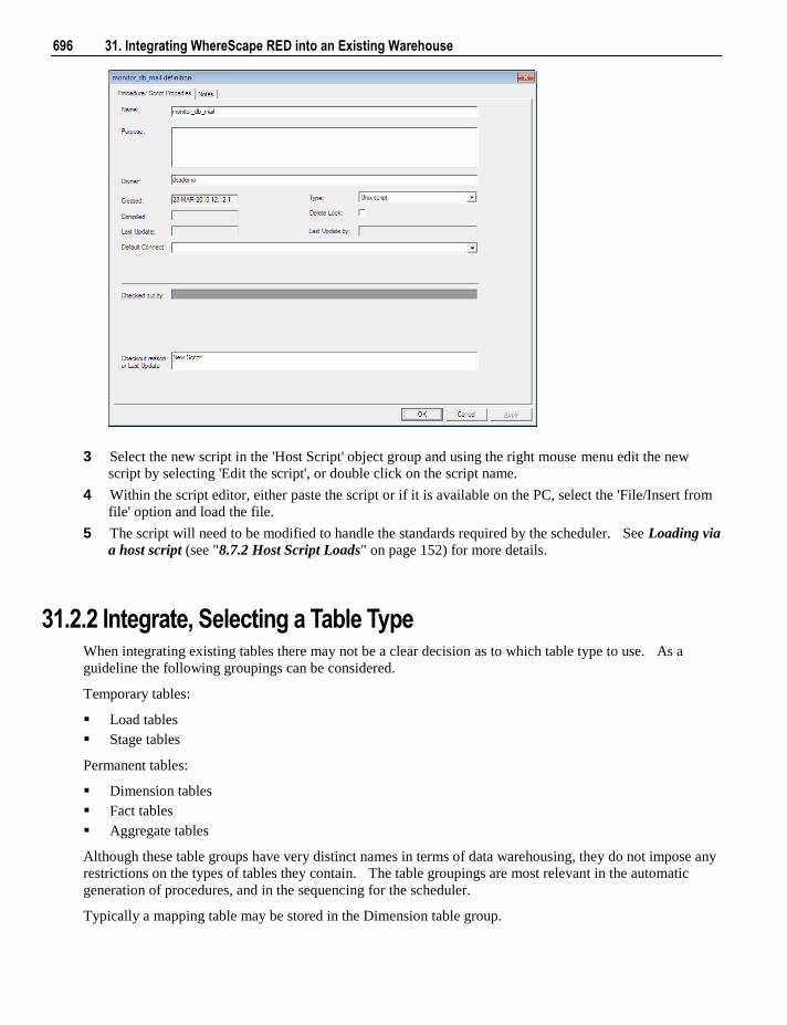
696 31. Integrating WhereScape RED into an Existing Warehouse
3 Select the new script in the 'Host Script' object group and using the right mouse menu edit the new
script by selecting 'Edit the script', or double click on the script name.
4 Within the script editor, either paste the script or if it is available on the PC, select the 'File/Insert from
file' option and load the file.
5 The script will need to be modified to handle the standards required by the scheduler. See Loading via
a host script (see "8.7.2 Host Script Loads" on page 152) for more details.
31.2.2 Integrate, Selecting a Table Type When integrating existing tables there may not be a clear decision as to which table type to use. As a
guideline the following groupings can be considered.
Temporary tables:
Load tables
Stage tables
Permanent tables:
Dimension tables
Fact tables
Aggregate tables
Although these table groups have very distinct names in terms of data warehousing, they do not impose any
restrictions on the types of tables they contain. The table groupings are most relevant in the automatic
generation of procedures, and in the sequencing for the scheduler.
Typically a mapping table may be stored in the Dimension table group.
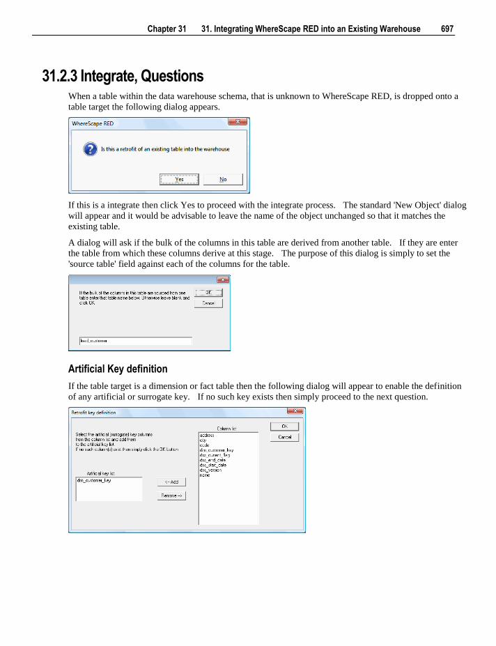
Chapter 31 31. Integrating WhereScape RED into an Existing Warehouse 697
31.2.3 Integrate, Questions When a table within the data warehouse schema, that is unknown to WhereScape RED, is dropped onto a
table target the following dialog appears.
If this is a integrate then click Yes to proceed with the integrate process. The standard 'New Object' dialog
will appear and it would be advisable to leave the name of the object unchanged so that it matches the
existing table.
A dialog will ask if the bulk of the columns in this table are derived from another table. If they are enter
the table from which these columns derive at this stage. The purpose of this dialog is simply to set the
'source table' field against each of the columns for the table.
Artificial Key definition
If the table target is a dimension or fact table then the following dialog will appear to enable the definition
of any artificial or surrogate key. If no such key exists then simply proceed to the next question.
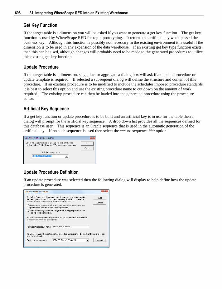
698 31. Integrating WhereScape RED into an Existing Warehouse
Get Key Function
If the target table is a dimension you will be asked if you want to generate a get key function. The get key
function is used by WhereScape RED for rapid prototyping. It returns the artificial key when passed the
business key. Although this function is possibly not necessary in the existing environment it is useful if the
dimension is to be used in any expansion of the data warehouse. If an existing get key type function exists,
then this can be used, although changes will probably need to be made to the generated procedures to utilize
this existing get key function.
Update Procedure
If the target table is a dimension, stage, fact or aggregate a dialog box will ask if an update procedure or
update template is required. If selected a subsequent dialog will define the structure and content of this
procedure. If an existing procedure is to be modified to include the scheduler imposed procedure standards
it is best to select this option and use the existing procedure name to cut down on the amount of work
required. The existing procedure can then be loaded into the generated procedure using the procedure
editor.
Artificial Key Sequence
If a get key function or update procedure is to be built and an artificial key is in use for the table then a
dialog will prompt for the artificial key sequence. A drop down list provides all the sequences defined for
this database user. This sequence is an Oracle sequence that is used in the automatic generation of the
artificial key. If no such sequence is used then select the *** no sequence *** option.
Update Procedure Definition
If an update procedure was selected then the following dialog will display to help define how the update
procedure is generated.
Chapter 31 31. Integrating WhereScape RED into an Existing Warehouse 699
As defined in this dialog box the scheduler needs specific parameters in order to control and run a
procedure. An existing procedure will not have these parameters. There are basically two forms of
generated procedure. The first option is to generate a procedure that looks much like a standard
WhereScape RED procedure and then manually insert the changes from the existing procedure. The
second option is to generate a wrapper procedure that calls the existing procedure. This second option will
still require manual changes to the procedure to return a valid return code and message.
Business Key definition
If a get key or update procedure has been selected a dialog will now prompt for the selection of the business
key from the table. Multiple columns may constitute the business key, but they must uniquely identify
each record in the table.
Index definition
Any indexes associated with the table will now be automatically defined and loaded into the metadata.
Changes may need to be made in terms of when the indexes are dropped and to set the 'Drop before update'
check box if appropriate and the scheduler is to be used to manage these indexes.
Procedure creation
If defined the get key and update procedures will now be generated. They will need to be manually edited
and compiled. See the section on integrating procedures (see "31.2.4 Integrate, Procedures" on page
698).
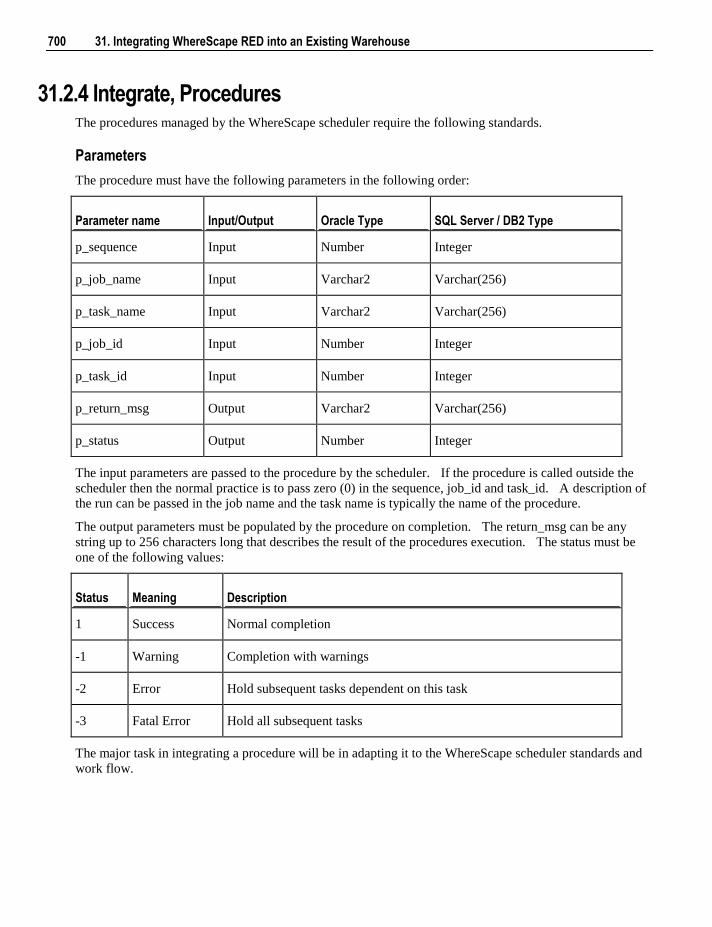
700 31. Integrating WhereScape RED into an Existing Warehouse
31.2.4 Integrate, Procedures The procedures managed by the WhereScape scheduler require the following standards.
Parameters
The procedure must have the following parameters in the following order:
Parameter name Input/Output Oracle Type SQL Server / DB2 Type
p_sequence Input Number Integer
p_job_name Input Varchar2 Varchar(256)
p_task_name Input Varchar2 Varchar(256)
p_job_id Input Number Integer
p_task_id Input Number Integer
p_return_msg Output Varchar2 Varchar(256)
p_status Output Number Integer
The input parameters are passed to the procedure by the scheduler. If the procedure is called outside the
scheduler then the normal practice is to pass zero (0) in the sequence, job_id and task_id. A description of
the run can be passed in the job name and the task name is typically the name of the procedure.
The output parameters must be populated by the procedure on completion. The return_msg can be any
string up to 256 characters long that describes the result of the procedures execution. The status must be
one of the following values:
Status Meaning Description
1 Success Normal completion
-1 Warning Completion with warnings
-2 Error Hold subsequent tasks dependent on this task
-3 Fatal Error Hold all subsequent tasks
The major task in integrating a procedure will be in adapting it to the WhereScape scheduler standards and
work flow.
Chapter 31 31. Integrating WhereScape RED into an Existing Warehouse 701
31.2.5 Integrate, Views When integrating views an additional step is required if you want WhereScape RED to be able to recreate
the view.
The view will be mapped correctly and the 'Get Key' function can still be built. This step is only required
if the view is to be re-created.
Change the source column on the artificial key to match the artificial key in the table from which the view
was created.
31.2.6 Integrate, WhereScape Tables When integrating WhereScape generated tables and views a number of additional considerations need to be
taken.
The Dimension tables and views make use of secondary business key columns such as
dss_source_system_key, dss_current_flag, dss_end_date, dss_version to assist in handling various forms of
slowly changing dimensions and non conformance. These secondary business keys need to be flagged as
such against the dimension.
Change the properties of all such columns. The key type should be set to 1, and the primary business key
check box should be set.

Index 703
1
1. Overview ................................................. 1
10. Staging ............................................... 195
10.1 Building the Stage Table ......... 195, 196
10.2 Generating the Staging Update
Procedure ............................. 195, 198, 199
10.3 Tuning the Staging Update Process 195,
210
10.4 Stage Table Column Properties ....... 211
10.5 Stage Table Column Transformations
............................................................. 216
11. Data Store Objects ............................. 217
11.1 Data Store Object Overview ............ 218
11.2 Building a Data Store Object ... 218, 220
11.3 Generating the Data Store Update
Procedure ....................... 73, 218, 223, 224
11.4 Data Store Artificial Keys ............... 235
11.5 Data Store Column Properties ......... 237
11.6 Data Store Object Column
Transformations ................................... 240
12. Normalized Tables ............................ 241
12.1 Normalized Tables Overview .......... 242
12.2 Building a Normalized Table .. 242, 244
12.3 Generating the Normalized Update
Procedure ............. 222, 242, 246, 247, 248
12.4 Normalized Table Artificial Keys ..................................................... 243, 260
12.5 Normalized Table Column Properties
............................................................. 263
12.6 Normalized Table Column
Transformations ................................... 267
13. Fact Tables ........................................ 269
13.1 Detail Fact Tables ................ 269, 270
13.1.1 Creating Detail Fact Tables .......... 270
13.2 Rollup or Combined Fact Tables .... 269,
271
13.2.1 Creating Rollup Fact Tables ......... 272
13.3 KPI Fact Tables ....................... 269, 273
13.3.1 Creating the KPI Dimension ........ 273
13.3.2 Creating KPI Fact Tables ............. 274
13.3.3 Setup of KPI Fact Tables ............. 275
13.3.3.1 KPI Setup .................................. 275
13.4 Snapshot Fact Tables ............... 269, 281
13.4.1 Creating Snapshot Fact Tables ..... 281
13.5 Slowly Changing Fact Tables.. 269, 281
13.5.1 Creating Slowly Changing Fact
Tables ................................................... 282
13.6 Partitioned Fact Tables ............ 269, 282
13.6.1 Creating a Partitioned Fact Table in
SQL Server .......................................... 283
13.6.2 Creating a Partitioned Fact Table in
Oracle ................................................... 287
13.6.3 Creating a Partitioned Fact Table in
DB2 ...................................................... 291
13.7 Fact Table Column Properties ......... 295
13.8 Fact Table Language Mapping ........ 299
14. Aggregation ....................................... 301
14.1 Creating an Aggregate Table ........... 301
14.1.1 Change an Aggregates Default Look
Back Days ............................................ 304
14.2 Creating an Aggregate Summary Table
............................................................. 304
15. Views ................................................. 307
15.1 Creating a Dimension View ............ 308
15.1.1 View Column Re-mapping ........... 312
15.2 Non-Dimension Object Views ........ 313
15.3 Creating a Custom View ................. 316
15.4 Dimension View Language Mapping
............................................................. 318
16. Analysis Services OLAP Cubes ........ 319
16.1 Overview ......................................... 319
16.2 Defining an OLAP Cube ................. 320
16.3 Inspecting and Modifying Advanced
Cube Properties .................................... 323
16.4 Creating an OLAP Cube on the
Analysis Services Server ..................... 325
16.5 Cube Objects ................................... 326
16.5.1 Properties ...................................... 326
16.5.10 Measure Group Dimensions ....... 353
Index
704 RED User Guide
16.5.2 Measure Groups ............................ 330
16.5.3 Measure Group Processing /
Partitions .............................................. 332
16.5.4 Measure Group Partitions ............. 335
16.5.5 Measures ....................................... 338
16.5.6 Calculations .................................. 341
16.5.7 Key Performance Indicators ......... 344
16.5.8 Actions .......................................... 347
16.5.9 Cube Dimensions .......................... 351
16.6 Dimension Objects .......................... 356
16.6.1 Dimension Overview .................... 356
16.6.2 Dimension Attributes .................... 359
16.6.3 Attribute Relationships ................. 362
16.6.4 Dimension Hierarchies ................. 364
16.6.5 Dimension User Defined Hierarchy
Levels ................................................... 366
16.7 Changing OLAP Cubes ................... 368
16.8 Retrofitting an OLAP Object ... 370, 677
17. Exporting Data ................................... 375
17.1 Building an Export Object ............... 375
17.2 File Attributes .................................. 378
17.2.1 Export Object File Attributes Screen
............................................................. 380
17.3 Export Column Attributes ............... 381
17.3.1 Export Column Attributes Screen . 382
17.4 Host Script Exports .......................... 383
18. MicroStrategy Projects ...................... 385
18.1 MicroStrategy Prerequisites ............ 385
18.2 Building MicroStrategy Projects ..... 385
19. Transformations .............. 159, 216, 387
19.1 Column Transformations ............ 387
19.1.1 Column Transformation Properties
..................................................... 388, 400
19.1.2 Load Table Column Transformations ......... 159, 387, 389, 390
19.1.2.1 Database Link During Load
Transformations ................................... 391
19.1.2.2 File During Load Transformations
............................................................. 393
19.1.2.3 After Load Transformations ...... 393
19.2 Database Functions .......................... 393
19.3 Re-usable Transformations .............. 393
19.3.1 Creating a New Re-usable
Transformation ............................. 394, 398
19.3.1.1 Specify the Name of the
Transformation ..................................... 394
19.3.1.2 Enter Re-usable Transformation
Metadata............................................... 395
19.3.1.3 Define the Transformation Model
............................................................. 396
19.3.1.4 Completed Re-usable
Transformation ..................................... 397
19.3.2 Changing a Re-usable Transformation398
19.3.2.1 Applying Changes to Dependant
Transformations ................................... 399
19.3.3 Using Re-usable Transformations 400
2
2. Design Introduction ................................. 7
20. Procedures and Scripts ......... 393, 401
20.1 Procedure Generation ...................... 402
20.10 Script Editing ................................. 427
20.11 Script Testing ................................ 428
20.12 Script Syntax ................................. 428
20.13 Templates ...................................... 430
20.2 Procedure Editing ............................ 405
20.3 Procedure Loading and Saving ........ 408
20.4 Procedure Comparisons ................... 409
20.5 Procedure Compilation .................... 410
20.6 Procedure Running .......................... 410
20.7 Procedure Syntax ............................. 411
20.8 Procedure Properties ........................ 412
20.9 Script Generation ............................. 413
20.9.1 Script Generation (Windows/SQL
Server) .................................................. 413
20.9.2 Script Generation (Unix/Oracle) .. 417
20.9.3 Script Generation (Windows/Oracle)
............................................................. 421
20.9.4 Script Generation (Windows/DB2)
............................................................. 424
21. Scheduler ........................................... 431
21.1 Scheduler Options ........................... 432
21.2 Scheduler States .............................. 435
21.3 Scheduling a Job .............................. 437
21.4 Editing Jobs ..................................... 445
21.5 Deleting Job Logs ............................ 446
21.6 Monitoring the Database and Jobs .. 447
21.6.1 Database Monitoring .................... 447
21.6.2 Job Monitoring ............................. 449
21.7 Stand Alone Scheduler Maintenance
............................................................. 454
22. Indexes............................................... 457
22.1 Index Definition .............................. 458
Index 705
22.2 Index Storage Properties ................. 464
22.2.1 Index Storage Screen - SQL Server.......................................... 464, 465
22.2.2 Index Storage Screen - Oracle ..... 464,
466
22.2.3 Index Storage Screen - DB2 . 464, 467
22.3 Index Menu Options ........................ 468
23. Documentation and Diagrams ........... 469
23.1 Creating Documentation .................. 469
23.2 Batch Documentation Creation ....... 472
23.3 Reading the Documentation .... 469, 473
23.4 Diagrams ......................................... 473
23.4.1 Star Schema diagram .................... 476
23.4.2 Track Back diagram ..................... 477
23.4.3 Data Join Track Back diagram ..... 480
23.4.4 Track Forward diagram ................ 481
23.4.5 Linked Tables diagram ................. 482
23.4.6 Job Dependencies diagram ........... 483
23.5 Query Tool Access .................. 469, 485
24. Reports .............................................. 487
24.1 Dimension-Fact Matrix ................... 488
24.2 OLAP Dimension-Cube Matrix ...... 489
24.3 Dimension Views of a Specified
Dimension ............................................ 490
24.4 Column Reports ............................... 491
24.4.1 Columns without Comments ........ 492
24.4.2 All Column Transformations ........ 494
24.4.3 Re-Usable Column Transformations
............................................................. 495
24.4.4 Column Track-Back ..................... 496
24.5 Table Reports .................................. 497
24.5.1 Tables without Comments ............ 498
24.5.2 Load Tables by Connection .......... 499
24.5.3 Records that failed a Dimension Join
............................................................. 500
24.5.4 External Source Table/files .......... 502
24.6 Procedure Reports ........................... 502
24.6.1 Modified Procedures .................... 503
24.6.2 Custom Procedures ....................... 504
24.7 Index Reports .................................. 504
24.7.1 Modified Indexes .......................... 505
24.8 Object Reports ................................. 506
24.8.1 Objects-Project Matrix ................. 507
24.8.2 Modified Objects (excluding indexes)
............................................................. 509
24.8.3 Objects Checked-out .................... 511
24.8.4 Loaded or Imported Objects ......... 512
24.9 Job Reports ...................................... 513
24.9.1 Object-Job Matrix ........................ 514
24.9.2 Jobs with an Object ...................... 516
24.9.3 Tasks of a Job ............................... 517
24.9.4 Object Performance History ......... 518
24.9.5 Job Performance History .............. 519
24.9.6 Task Performance History ............ 520
25. Validate ............................................. 521
25.1 Validate Meta-data .......................... 521
25.10 List Procedures not related to a Table
............................................................. 526
25.11 Compare Meta-data Repository to
another ................................................. 527
25.12 Compare Meta-data Indexes to
Database ............................................... 530
25.13 List Duplicate Business Key Columns
............................................................. 531
25.14 Query Data Warehouse Objects .... 532
25.2 Validate Workflow Data ................. 522
25.3 Validate Table Create Status ........... 522
25.4 Validate Load Table Status ............. 522
25.5 Validate Index Status ...................... 522
25.6 Validate Procedure Status ............... 523
25.7 List Meta-data Tables not in the
Database ............................................... 523
25.8 List Database Tables not in the
Meta-data ............................................. 524
25.9 List Tables with no related Procedures
or Scripts .............................................. 525
26. Promoting Between Environments .... 533
26.1 Applications .................................... 534
26.1.1 Application Creation .................... 535
26.1.2 Application Loading ..................... 538
26.2 Importing Object Metadata ............. 539
26.3 Importing Language Files ............... 540
26.4 Data Warehouse Testing ................. 542
26.5 Creating and Loading Applications
from the Command Line ...................... 545
27. Backing Up and Restoring Metadata 533,
547
27.1 Backup using DB Routines ............. 548
27.2 Restoring DB Backups .................... 551
27.3 Unloading Metadata ........................ 555
27.4 Loading an Unload .......................... 556
28. Altering Metadata .............................. 559
28.1 Validating Tables ............................ 560
28.2 Validating Source (Load) Tables .... 562
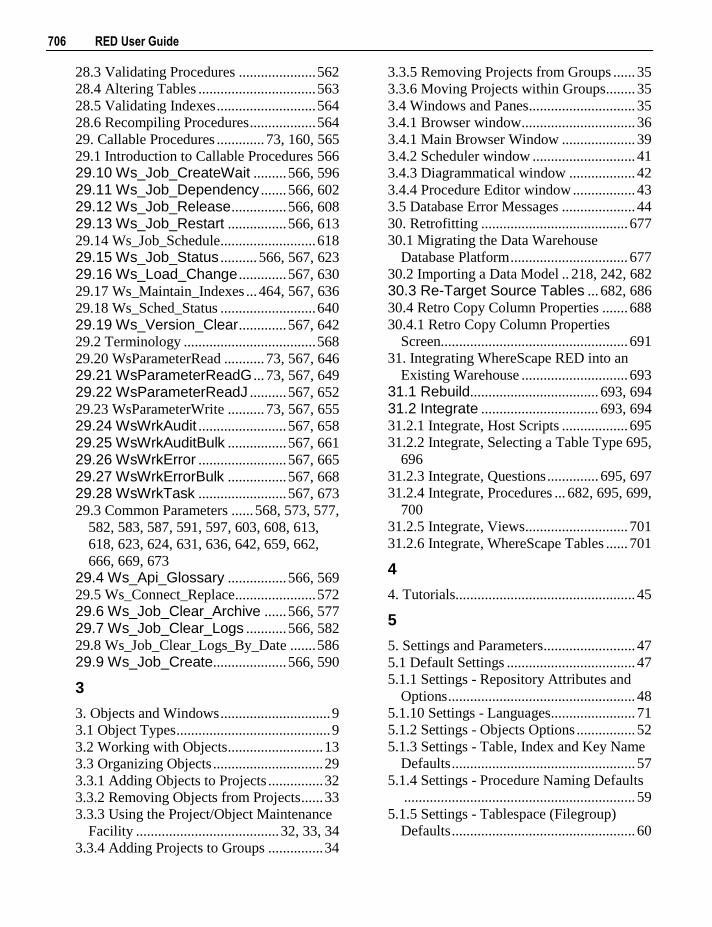
706 RED User Guide
28.3 Validating Procedures ..................... 562
28.4 Altering Tables ................................ 563
28.5 Validating Indexes ........................... 564
28.6 Recompiling Procedures .................. 564
29. Callable Procedures ............. 73, 160, 565
29.1 Introduction to Callable Procedures 566
29.10 Ws_Job_CreateWait ......... 566, 596
29.11 Ws_Job_Dependency ....... 566, 602
29.12 Ws_Job_Release ............... 566, 608
29.13 Ws_Job_Restart ................ 566, 613
29.14 Ws_Job_Schedule .......................... 618
29.15 Ws_Job_Status .......... 566, 567, 623
29.16 Ws_Load_Change ............. 567, 630
29.17 Ws_Maintain_Indexes ... 464, 567, 636
29.18 Ws_Sched_Status .......................... 640
29.19 Ws_Version_Clear ............. 567, 642
29.2 Terminology .................................... 568
29.20 WsParameterRead ........... 73, 567, 646
29.21 WsParameterReadG ... 73, 567, 649
29.22 WsParameterReadJ .......... 567, 652
29.23 WsParameterWrite .......... 73, 567, 655
29.24 WsWrkAudit ........................ 567, 658
29.25 WsWrkAuditBulk ................ 567, 661
29.26 WsWrkError ........................ 567, 665
29.27 WsWrkErrorBulk ................ 567, 668
29.28 WsWrkTask ........................ 567, 673
29.3 Common Parameters ...... 568, 573, 577,
582, 583, 587, 591, 597, 603, 608, 613,
618, 623, 624, 631, 636, 642, 659, 662,
666, 669, 673
29.4 Ws_Api_Glossary ................ 566, 569
29.5 Ws_Connect_Replace ...................... 572
29.6 Ws_Job_Clear_Archive ...... 566, 577
29.7 Ws_Job_Clear_Logs ........... 566, 582
29.8 Ws_Job_Clear_Logs_By_Date ....... 586
29.9 Ws_Job_Create .................... 566, 590
3
3. Objects and Windows .............................. 9
3.1 Object Types .......................................... 9
3.2 Working with Objects .......................... 13
3.3 Organizing Objects .............................. 29
3.3.1 Adding Objects to Projects ............... 32
3.3.2 Removing Objects from Projects ...... 33
3.3.3 Using the Project/Object Maintenance
Facility ....................................... 32, 33, 34
3.3.4 Adding Projects to Groups ............... 34
3.3.5 Removing Projects from Groups ...... 35
3.3.6 Moving Projects within Groups ........ 35
3.4 Windows and Panes ............................. 35
3.4.1 Browser window ............................... 36
3.4.1 Main Browser Window .................... 39
3.4.2 Scheduler window ............................ 41
3.4.3 Diagrammatical window .................. 42
3.4.4 Procedure Editor window ................. 43
3.5 Database Error Messages .................... 44
30. Retrofitting ........................................ 677
30.1 Migrating the Data Warehouse
Database Platform ................................ 677
30.2 Importing a Data Model .. 218, 242, 682
30.3 Re-Target Source Tables ... 682, 686
30.4 Retro Copy Column Properties ....... 688
30.4.1 Retro Copy Column Properties
Screen................................................... 691
31. Integrating WhereScape RED into an
Existing Warehouse ............................. 693
31.1 Rebuild................................... 693, 694
31.2 Integrate ................................ 693, 694
31.2.1 Integrate, Host Scripts .................. 695
31.2.2 Integrate, Selecting a Table Type 695,
696
31.2.3 Integrate, Questions .............. 695, 697
31.2.4 Integrate, Procedures ... 682, 695, 699,
700
31.2.5 Integrate, Views ............................ 701
31.2.6 Integrate, WhereScape Tables ...... 701
4
4. Tutorials................................................. 45
5
5. Settings and Parameters ......................... 47
5.1 Default Settings ................................... 47
5.1.1 Settings - Repository Attributes and
Options ................................................... 48
5.1.10 Settings - Languages....................... 71
5.1.2 Settings - Objects Options ................ 52
5.1.3 Settings - Table, Index and Key Name
Defaults .................................................. 57
5.1.4 Settings - Procedure Naming Defaults
............................................................... 59
5.1.5 Settings - Tablespace (Filegroup)
Defaults .................................................. 60
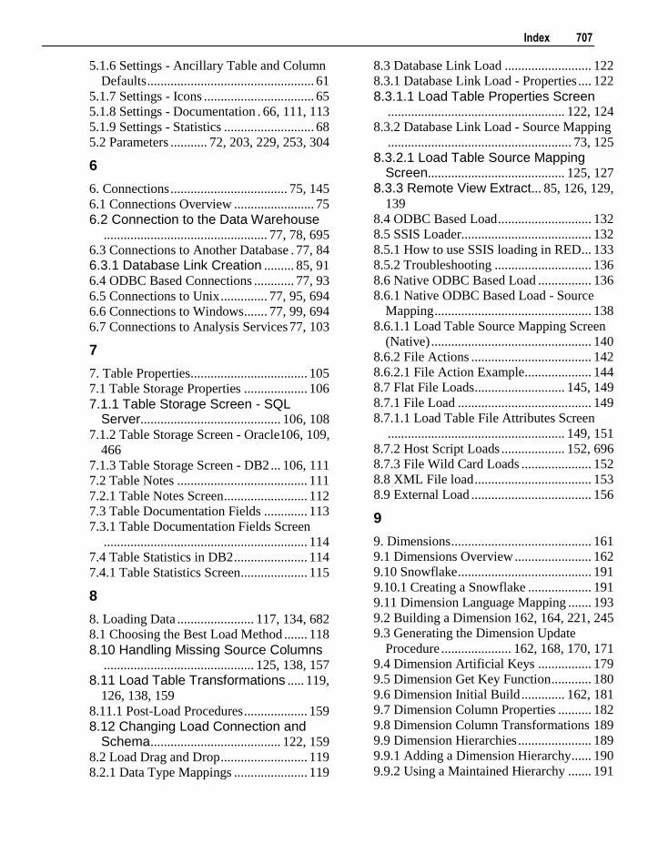
Index 707
5.1.6 Settings - Ancillary Table and Column
Defaults .................................................. 61
5.1.7 Settings - Icons ................................. 65
5.1.8 Settings - Documentation . 66, 111, 113
5.1.9 Settings - Statistics ........................... 68
5.2 Parameters ........... 72, 203, 229, 253, 304
6
6. Connections ................................... 75, 145
6.1 Connections Overview ........................ 75
6.2 Connection to the Data Warehouse ................................................. 77, 78, 695
6.3 Connections to Another Database . 77, 84
6.3.1 Database Link Creation ......... 85, 91
6.4 ODBC Based Connections ............ 77, 93
6.5 Connections to Unix .............. 77, 95, 694
6.6 Connections to Windows ....... 77, 99, 694
6.7 Connections to Analysis Services 77, 103
7
7. Table Properties ................................... 105
7.1 Table Storage Properties ................... 106
7.1.1 Table Storage Screen - SQL Server.......................................... 106, 108
7.1.2 Table Storage Screen - Oracle106, 109,
466
7.1.3 Table Storage Screen - DB2 ... 106, 111
7.2 Table Notes ....................................... 111
7.2.1 Table Notes Screen ......................... 112
7.3 Table Documentation Fields ............. 113
7.3.1 Table Documentation Fields Screen
............................................................. 114
7.4 Table Statistics in DB2 ...................... 114
7.4.1 Table Statistics Screen .................... 115
8
8. Loading Data ....................... 117, 134, 682
8.1 Choosing the Best Load Method ....... 118
8.10 Handling Missing Source Columns ............................................. 125, 138, 157
8.11 Load Table Transformations ..... 119,
126, 138, 159
8.11.1 Post-Load Procedures ................... 159
8.12 Changing Load Connection and Schema ....................................... 122, 159
8.2 Load Drag and Drop .......................... 119
8.2.1 Data Type Mappings ...................... 119
8.3 Database Link Load .......................... 122
8.3.1 Database Link Load - Properties .... 122
8.3.1.1 Load Table Properties Screen ..................................................... 122, 124
8.3.2 Database Link Load - Source Mapping
....................................................... 73, 125
8.3.2.1 Load Table Source Mapping Screen ......................................... 125, 127
8.3.3 Remote View Extract ... 85, 126, 129,
139
8.4 ODBC Based Load ............................ 132
8.5 SSIS Loader....................................... 132
8.5.1 How to use SSIS loading in RED ... 133
8.5.2 Troubleshooting ............................. 136
8.6 Native ODBC Based Load ................ 136
8.6.1 Native ODBC Based Load - Source
Mapping ............................................... 138
8.6.1.1 Load Table Source Mapping Screen
(Native) ................................................ 140
8.6.2 File Actions .................................... 142
8.6.2.1 File Action Example .................... 144
8.7 Flat File Loads ........................... 145, 149
8.7.1 File Load ........................................ 149
8.7.1.1 Load Table File Attributes Screen
..................................................... 149, 151
8.7.2 Host Script Loads ................... 152, 696
8.7.3 File Wild Card Loads ..................... 152
8.8 XML File load ................................... 153
8.9 External Load .................................... 156
9
9. Dimensions .......................................... 161
9.1 Dimensions Overview ....................... 162
9.10 Snowflake ........................................ 191
9.10.1 Creating a Snowflake ................... 191
9.11 Dimension Language Mapping ....... 193
9.2 Building a Dimension 162, 164, 221, 245
9.3 Generating the Dimension Update
Procedure ..................... 162, 168, 170, 171
9.4 Dimension Artificial Keys ................ 179
9.5 Dimension Get Key Function ............ 180
9.6 Dimension Initial Build ............. 162, 181
9.7 Dimension Column Properties .......... 182
9.8 Dimension Column Transformations 189
9.9 Dimension Hierarchies ...................... 189
9.9.1 Adding a Dimension Hierarchy ...... 190
9.9.2 Using a Maintained Hierarchy ....... 191
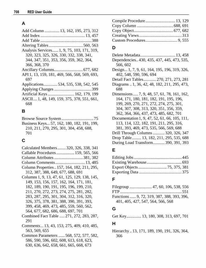
708 RED User Guide
A
Add Column .............. 13, 162, 195, 273, 312
Add Index .......................................... 13, 457
Add Table ................................................ 388
Altering Tables ................................ 560, 563
Analysis Services ...... 1, 9, 75, 103, 171, 319,
320, 323, 325, 326, 330, 332, 338, 341,
344, 347, 351, 353, 356, 359, 362, 364,
366, 368, 370
Ancillary Columns ........................... 677, 682
API 1, 13, 159, 181, 469, 566, 568, 569, 693,
697
Applications ............. 534, 535, 538, 542, 545
Applying Changes ................................... 399
Artificial Keys ......................... 162, 179, 199
ASCII .... 1, 48, 149, 159, 375, 378, 551, 661,
668
B
Browse Source System .............................. 75
Business Keys ... 57, 162, 180, 182, 191, 199,
210, 211, 270, 295, 301, 304, 458, 688,
701
C
Calculated Members ........ 320, 326, 338, 341
Callable Procedures ................. 159, 565, 566
Column Attributes ........................... 381, 382
Column Comments ............................ 13, 485
Column Properties .. 157, 164, 182, 211, 295,
312, 387, 388, 649, 677, 688, 691
Columns 1, 9, 13, 47, 61, 125, 129, 138, 145,
149, 153, 156, 157, 162, 164, 171, 181,
182, 189, 190, 191, 195, 196, 199, 210,
211, 270, 272, 273, 274, 275, 281, 282,
283, 287, 295, 301, 304, 312, 316, 320,
326, 375, 378, 381, 388, 390, 391, 393,
399, 458, 469, 473, 485, 559, 560, 562,
564, 677, 682, 686, 688, 697, 701
Combined Fact Table ..... 271, 272, 283, 287,
291
Comments ... 13, 43, 153, 275, 409, 410, 485,
563, 569, 655
Common Parameters ...... 568, 572, 577, 582,
586, 590, 596, 602, 608, 613, 618, 623,
630, 636, 642, 658, 661, 665, 668, 673
Compile Procedure ............................ 13, 129
Copy Column .................................. 688, 691
Copy Object ..................................... 677, 682
Creating Views ........................................ 313
Custom Procedures .............................. 9, 555
D
Delete Metadata ................................. 13, 458
Dependencies .. 430, 435, 437, 445, 473, 535,
566, 602
Design ... 1, 7, 9, 61, 164, 195, 196, 319, 326,
402, 548, 590, 596, 694
Detail Fact Tables ............ 270, 271, 273, 281
Diagrams .. 1, 36, 42, 48, 182, 211, 295, 473,
688
Dimensions ..... 7, 9, 48, 57, 61, 78, 161, 162,
164, 171, 180, 181, 182, 191, 195, 196,
199, 269, 270, 271, 272, 274, 275, 301,
304, 307, 308, 313, 320, 351, 356, 359,
362, 364, 366, 437, 473, 485, 682, 701
Documentation 1, 9, 47, 52, 61, 66, 105, 111,
113, 114, 122, 182, 191, 211, 295, 316,
381, 393, 469, 473, 535, 566, 569, 688
Drill Through Columns ........... 320, 326, 347
Drop Table ......... 13, 182, 211, 295, 535, 688
During Load Transform ........... 390, 391, 393
E
Editing Jobs ............................................. 445
Existing Warehouse ................................. 693
Export Objects ........................... 75, 375, 381
Exporting Data ........................................ 375
F
Filegroup ..................... 47, 60, 106, 538, 556
FTP .......................................................... 551
Functions ...... 9, 72, 319, 387, 388, 393, 396,
401, 405, 427, 547, 564, 566, 568
G
Get Key.............. 13, 180, 308, 313, 697, 701
H
Hierarchy .. 13, 171, 189, 190, 191, 326, 364,
366
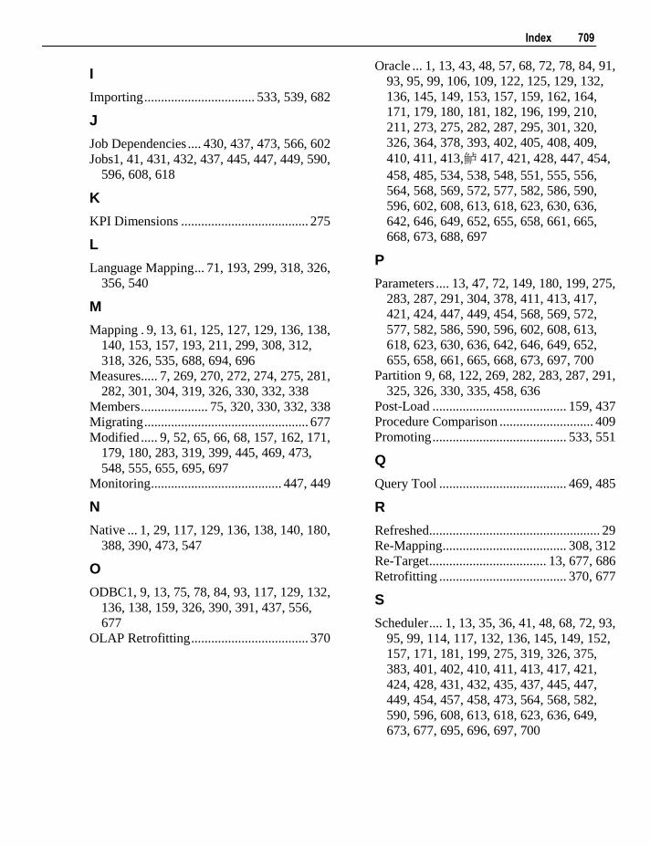
Index 709
I
Importing ................................. 533, 539, 682
J
Job Dependencies .... 430, 437, 473, 566, 602
Jobs1, 41, 431, 432, 437, 445, 447, 449, 590,
596, 608, 618
K
KPI Dimensions ...................................... 275
L
Language Mapping ... 71, 193, 299, 318, 326,
356, 540
M
Mapping . 9, 13, 61, 125, 127, 129, 136, 138,
140, 153, 157, 193, 211, 299, 308, 312,
318, 326, 535, 688, 694, 696
Measures ..... 7, 269, 270, 272, 274, 275, 281,
282, 301, 304, 319, 326, 330, 332, 338
Members .................... 75, 320, 330, 332, 338
Migrating ................................................. 677
Modified ..... 9, 52, 65, 66, 68, 157, 162, 171,
179, 180, 283, 319, 399, 445, 469, 473,
548, 555, 655, 695, 697
Monitoring ....................................... 447, 449
N
Native ... 1, 29, 117, 129, 136, 138, 140, 180,
388, 390, 473, 547
O
ODBC1, 9, 13, 75, 78, 84, 93, 117, 129, 132,
136, 138, 159, 326, 390, 391, 437, 556,
677
OLAP Retrofitting ................................... 370
Oracle ... 1, 13, 43, 48, 57, 68, 72, 78, 84, 91,
93, 95, 99, 106, 109, 122, 125, 129, 132,
136, 145, 149, 153, 157, 159, 162, 164,
171, 179, 180, 181, 182, 196, 199, 210,
211, 273, 275, 282, 287, 295, 301, 320,
326, 364, 378, 393, 402, 405, 408, 409,
410, 411, 413,鲈 417, 421, 428, 447, 454,
458, 485, 534, 538, 548, 551, 555, 556,
564, 568, 569, 572, 577, 582, 586, 590,
596, 602, 608, 613, 618, 623, 630, 636,
642, 646, 649, 652, 655, 658, 661, 665,
668, 673, 688, 697
P
Parameters .... 13, 47, 72, 149, 180, 199, 275,
283, 287, 291, 304, 378, 411, 413, 417,
421, 424, 447, 449, 454, 568, 569, 572,
577, 582, 586, 590, 596, 602, 608, 613,
618, 623, 630, 636, 642, 646, 649, 652,
655, 658, 661, 665, 668, 673, 697, 700
Partition 9, 68, 122, 269, 282, 283, 287, 291,
325, 326, 330, 335, 458, 636
Post-Load ........................................ 159, 437
Procedure Comparison ............................ 409
Promoting ........................................ 533, 551
Q
Query Tool ...................................... 469, 485
R
Refreshed ................................................... 29
Re-Mapping ..................................... 308, 312
Re-Target ................................... 13, 677, 686
Retrofitting ...................................... 370, 677
S
Scheduler .... 1, 13, 35, 36, 41, 48, 68, 72, 93,
95, 99, 114, 117, 132, 136, 145, 149, 152,
157, 171, 181, 199, 275, 319, 326, 375,
383, 401, 402, 410, 411, 413, 417, 421,
424, 428, 431, 432, 435, 437, 445, 447,
449, 454, 457, 458, 473, 564, 568, 582,
590, 596, 608, 613, 618, 623, 636, 649,
673, 677, 695, 696, 697, 700
710 RED User Guide
Schema ..... 1, 7, 9, 13, 36, 42, 48, 68, 75, 84,
106, 114, 122, 125, 138, 153, 159, 191,
195, 269, 326, 364, 454, 473, 551, 556,
564, 566, 569, 572, 577, 582, 586, 590,
596, 602, 608, 613, 618, 623, 630, 636,
642, 646, 649, 652, 655, 658, 661, 665,
668, 673, 677, 697
Slowly Changing Dimension .. 9, 57, 61, 164,
171, 182, 199, 211, 282, 295, 688, 701
Snowflake ............................................ 7, 191
SQL 1, 13, 48, 57, 60, 72, 75, 78, 84, 91, 99,
103, 106, 108, 122, 125, 129, 132, 136,
138, 145, 149, 153, 159, 162, 164, 171,
179, 180, 181, 182, 189, 199, 210, 211,
216, 273, 275, 282, 283, 295, 316, 320,
326, 338, 364, 378, 387, 388, 390, 391,
393, 396, 398, 408, 411, 413, 417, 421,
428, 454, 458, 485, 534, 535, 548, 551,
555, 556, 568, 569, 572, 577, 582, 586,
590, 596, 602, 608, 613, 618, 623, 630,
636, 642, 646, 649, 652, 655, 658, 661,
665, 668, 673, 688
Statistics ............. 68, 114, 115, 181, 210, 273
Storage 13, 60, 105, 106, 108, 109, 111, 136,
164, 196, 430, 458, 563
T
Tablespace ........... 47, 60, 106, 538, 556, 636
Transformations ...... 1, 9, 129, 156, 157, 159,
189, 199, 211, 216, 316, 387, 388, 390,
391, 393, 394, 395, 398, 399, 400, 437,
555, 688
Transforming ........................................... 195
U
Unix .... 9, 13, 48, 75, 95, 117, 132, 145, 149,
152, 401, 412, 413, 417, 428, 431, 435,
437, 447, 449, 548, 551, 694, 695
W
Wild Cards ............................... 152, 577, 586
X
XML ............................................ 9, 117, 153