1

What Broke Where For Distributed and Parallel

Applications — A Whodunit Story

Subrata Mitra

2

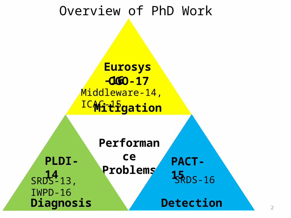
Overview of PhD Work

PerformanceProblems

Diagnosis

PLDI-14

SRDS-13, IWPD-16

Detection

PACT-15SRDS-16

Mitigation

Eurosys-16CGO-17

Middleware-14, ICAC-15

3

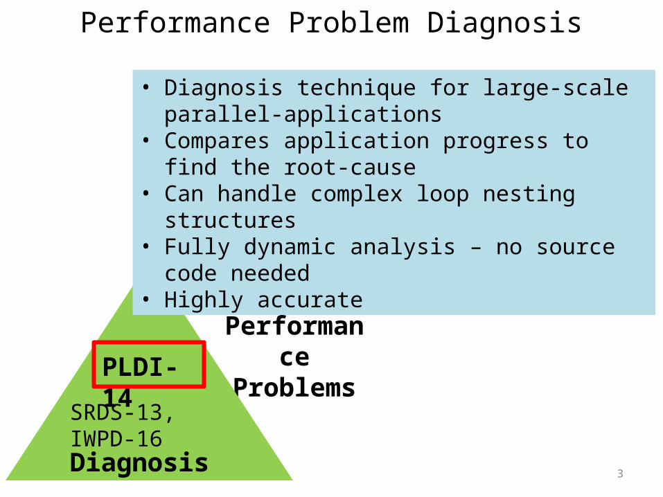
Performance Problem Diagnosis

PerformanceProblems

Diagnosis

PLDI-14

SRDS-13, IWPD-16

• Diagnosis technique for large-scale parallel-applications

• Compares application progress to find the root-cause• Can handle complex loop nesting structures• Fully dynamic analysis – no source code needed• Highly accurate

4

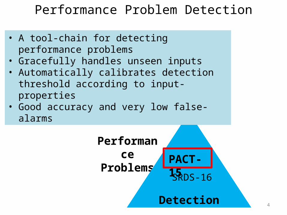
Performance Problem Detection

PerformanceProblems

Detection

PACT-15SRDS-16

• A tool-chain for detecting performance problems• Gracefully handles unseen inputs• Automatically calibrates detection threshold

according to input-properties• Good accuracy and very low false-alarms

5

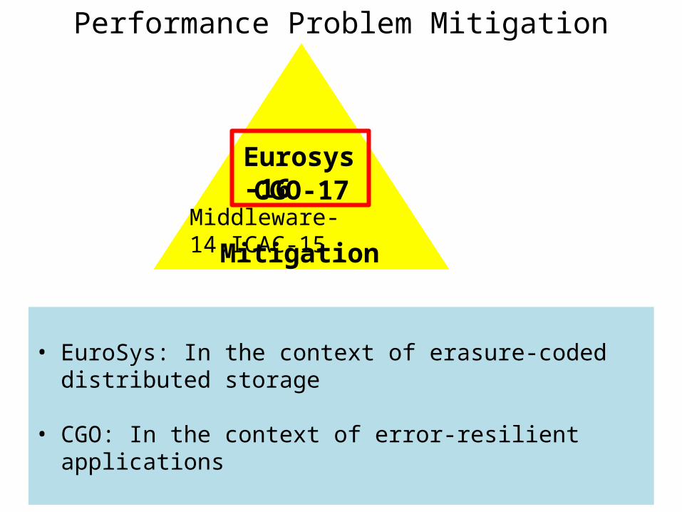
Performance Problem Mitigation

Mitigation

Eurosys-16CGO-17

Middleware-14,ICAC-15

• EuroSys: In the context of erasure-coded distributed storage

• CGO: In the context of error-resilient applications

6

Partial-Parallel-Repair (PPR):A Distributed Technique for Repairing

Erasure Coded Storage

Eurosys-2016

Subrata Mitra, Rajesh Panta (At&t), Moo Ryong Ra (At&t), Saurabh Bagchi

7

Need for storage redundancy

Data center storages are frequently affected by unavailability events

• Unplanned unavailability: - Component failures, network congestions, software glitches, power failures

• Planned unavailability: - Software/hardware updates, infrastructure maintenance

How storage redundancy helps ?

• Prevents permanent data loss (Reliability)• Keeps the data accessible to the user (Availability)

8

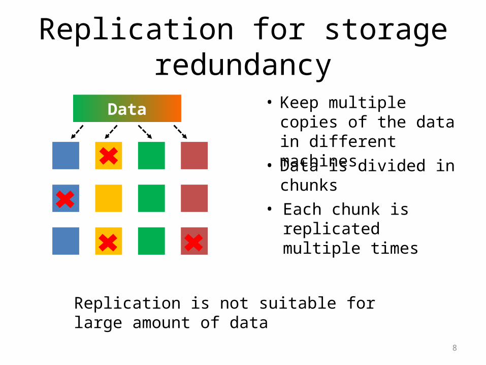
Replication for storage redundancy

• Keep multiple copies of the data in different machines

Data

• Data is divided in chunks

• Each chunk is replicated multiple times

Replication is not suitable for large amount of data

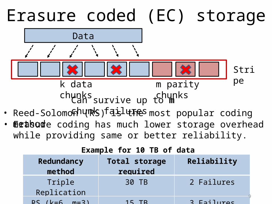
Erasure coded (EC) storage

• Reed-Solomon (RS) is the most popular coding method

Data

k data chunks m parity chunks

Stripe

Can survive up to m chunk failures

Redundancy method Total storage required ReliabilityTriple Replication 30 TB 2 Failures

RS (k=6, m=3) 15 TB 3 FailuresRS (k=12, m=4) 13.34 TB 4 Failures 9

Example for 10 TB of data

• Erasure coding has much lower storage overhead while providing same or better reliability.

10

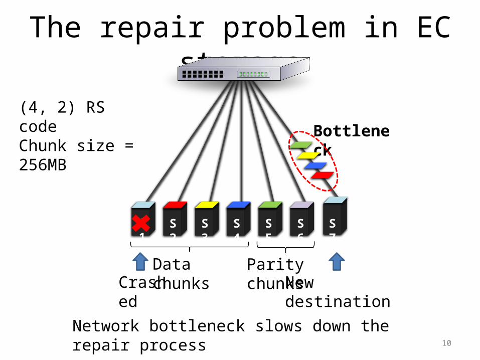
The repair problem in EC storage

Crashed New destination

S7S2 S3 S4 S5 S6S1

Data chunks Parity chunks

(4, 2) RS codeChunk size = 256MB

Bottleneck

Network bottleneck slows down the repair process

11

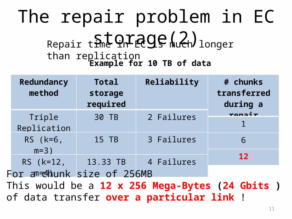
The repair problem in EC storage(2)Repair time in EC is much longer than replication

Redundancy method

Total storage required

Reliability

Triple Replication 30 TB 2 Failures

RS (k=6, m=3) 15 TB 3 Failures

RS (k=12, m=4) 13.33 TB 4 Failures

Example for 10 TB of data

# chunks transferred during

a repair

1

6

12

For a chunk size of 256MBThis would be a 12 x 256 Mega-Bytes (24 Gbits ) of data transfer over a particular link !

12

What triggers a repair ?

• Monitoring process finds unavailable chunks - Regular repairs- Chunk is re-created in a new server

• Client finds missing or corrupted chunks- Degraded reads- Chunk is re-created in the client- On the critical path of the user application

13

Existing solutions• Keep additional parities: Need additional storage Huang et al. (ATC-2012), Sathiamoorthy et al. (VLDB-2013) • Mix of both replication and erasure code: Higher storage overhead

than EC Xia et al. (FAST-2015), Ma et al. (INFOCOM-2013)

• Repair friendly codes: Restricted parameters Khan et al. (FAST-2012), Xiang et al. (SIGMETRICS-2010), Hu et al. (FAST-2012), Rashmi et al. (SIGCOMM-2014)

• Delay repairs: Depends on policy. Immediate repair needed for degraded reads

Silberstein et al. (SYSTOR-2014)

14

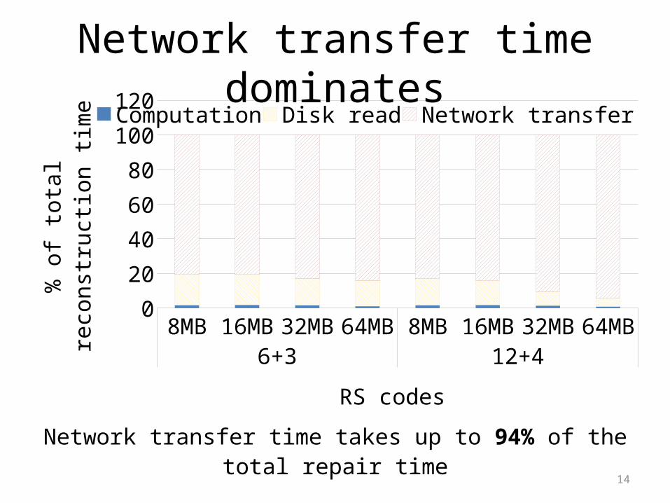
8MB 16MB 32MB 64MB 8MB 16MB 32MB 64MB6+3 12+4

0

20

40

60

80

100

120Computation Disk read Network transfer

RS codes

% o

f tot

al re

cons

truc

tion

time

Network transfer time takes up to 94% of the total repair time

Network transfer time dominates

15

Our solution approachWe introduce: Partial Parallel Repair (PPR)

• A distributed repair technique – targeted to reduce network transfer time

• No additional storage

• No restrictions on the code

• Significantly lower repair time

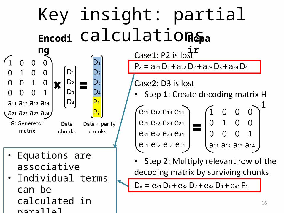
16

Key insight: partial calculationsEncoding Repair

• Equations are associative• Individual terms can be

calculated in parallel

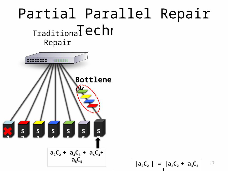
17

Partial Parallel Repair Technique

S7S2 S3 S4 S5 S6S1

Traditional Repair

a2C2 + a3C3 + a4C4+ a5C5

Bottleneck

Partial Parallel Repair

S7S2 S3 S4 S5 S6S1

a2C2 a4C4a2C2 + a3C3 a4C4 + a5C5a2C2 + a3C3+ a4C4 + a5C5

|a2C2 | = |a2C2 + a3C3 |

18

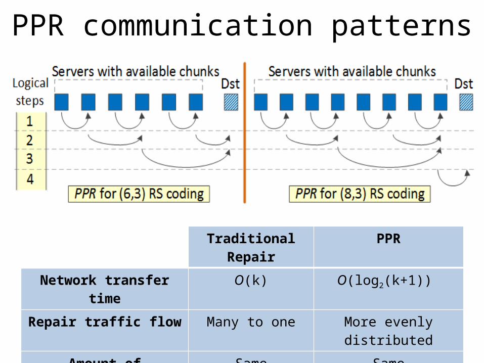
PPR communication patterns

Traditional Repair PPR

Network transfer time O(k) O(log2(k+1))

Repair traffic flow Many to one More evenly distributedAmount of transferred data Same Same

19

PPR

tim

e/ T

radi

tiona

l tim

e

k

1.2

1.0

0.8

0.6

0.4

0.2

0.02 4 6 8 10 12 14 16 18 20

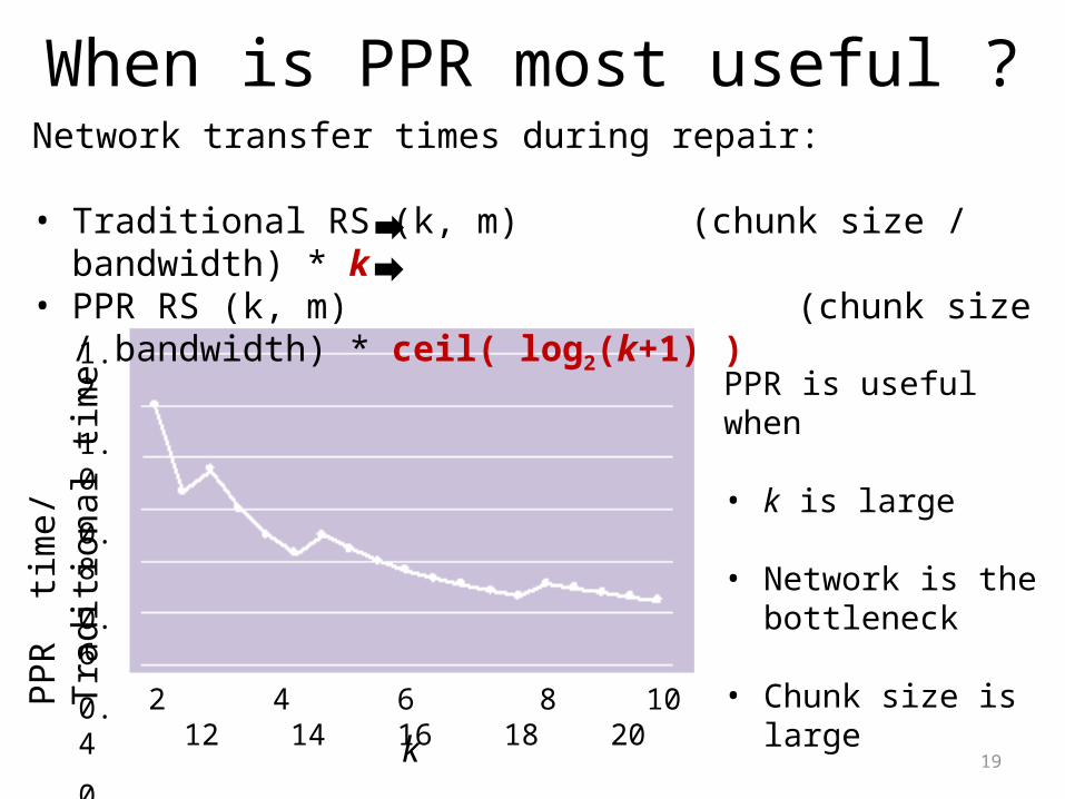
When is PPR most useful ?Network transfer times during repair:

• Traditional RS (k, m) (chunk size / bandwidth) * k• PPR RS (k, m) (chunk size / bandwidth) * ceil( log2(k+1) )

PPR is useful when

• k is large

• Network is the bottleneck

• Chunk size is large

20

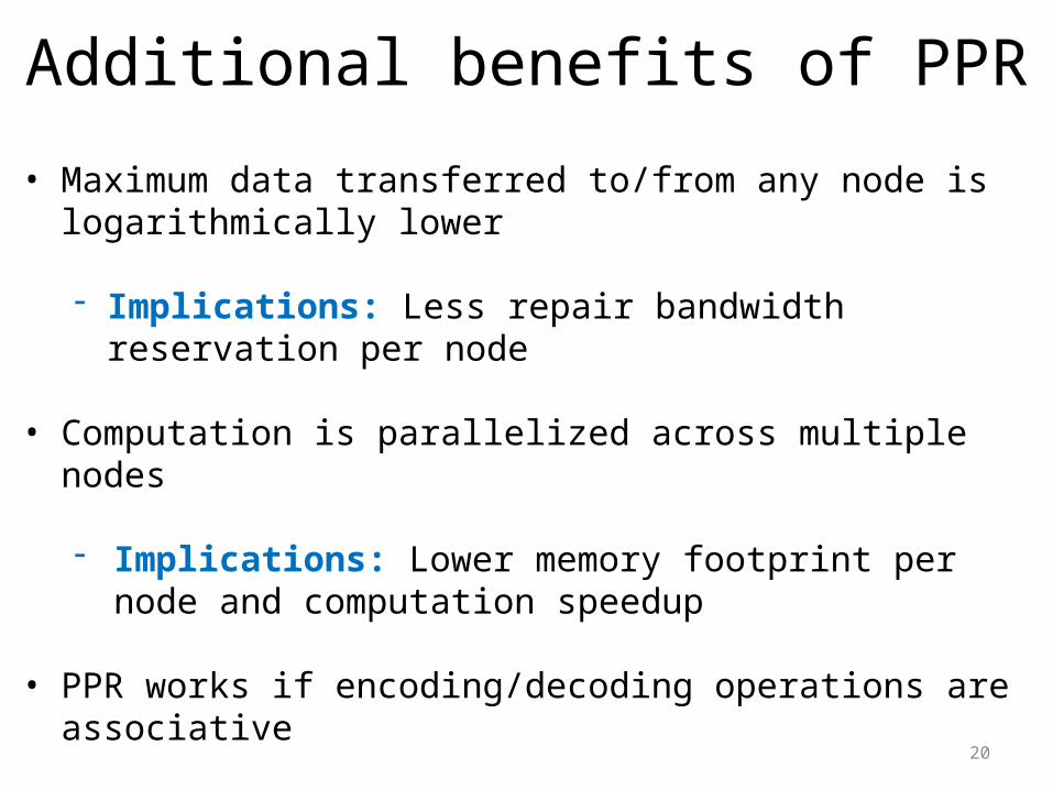
Additional benefits of PPR

• Maximum data transferred to/from any node is logarithmically lower

- Implications: Less repair bandwidth reservation per node

• Computation is parallelized across multiple nodes

- Implications: Lower memory footprint per node and computation speedup

• PPR works if encoding/decoding operations are associative

- Implications: Compatible to a wide range of codes including RS, LRC, RS-Hitchhiker, Rotated-RS etc.

21

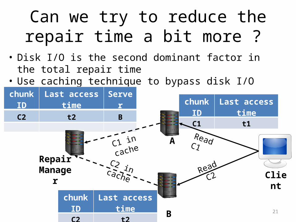
Can we try to reduce the repair time a bit more ?

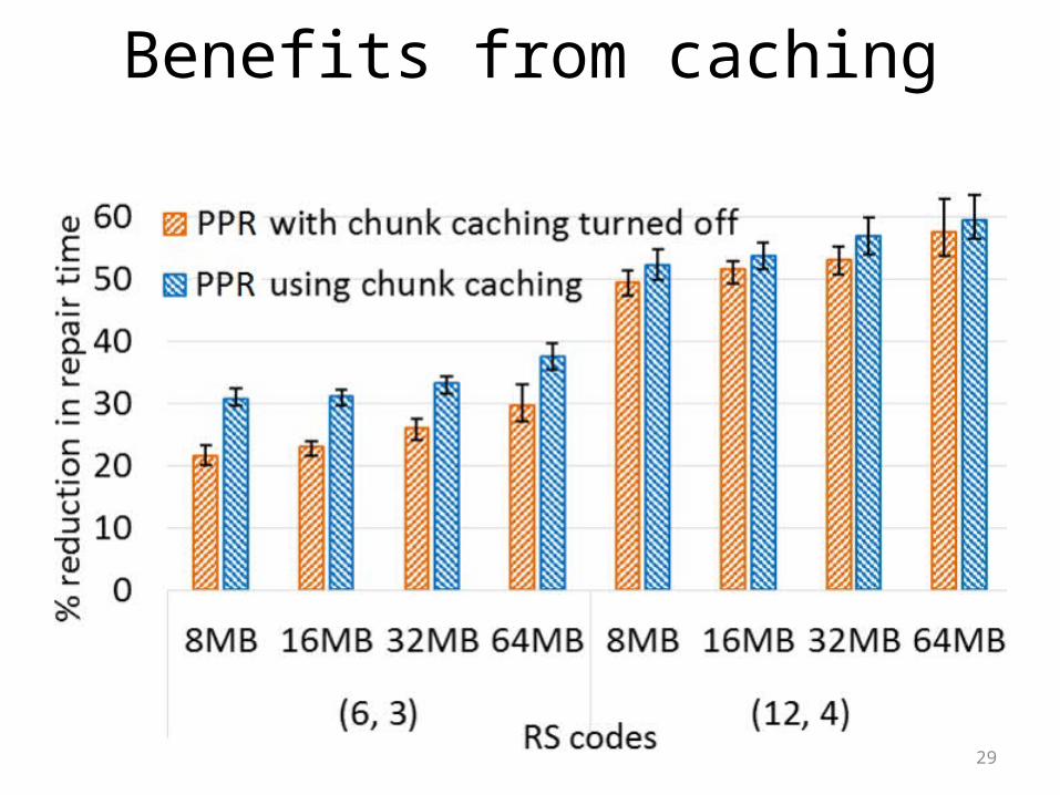
• Disk I/O is the second dominant factor in the total repair time• Use caching technique to bypass disk I/O time

chunkID Last access timeC1 t1

chunkID Last access time ServerC1 t1 A

Client

B

A

Repair Manager

Read C1

Read C2C2 in cache

C1 in cache

chunkID Last access timeC2 t2

C2 t2 B

22

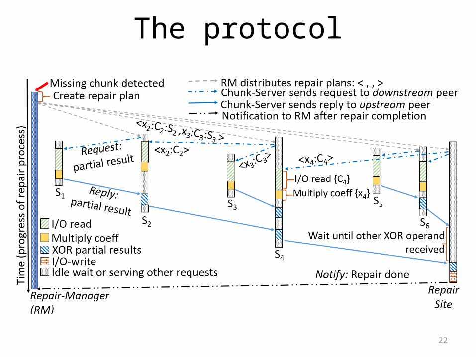
The protocol

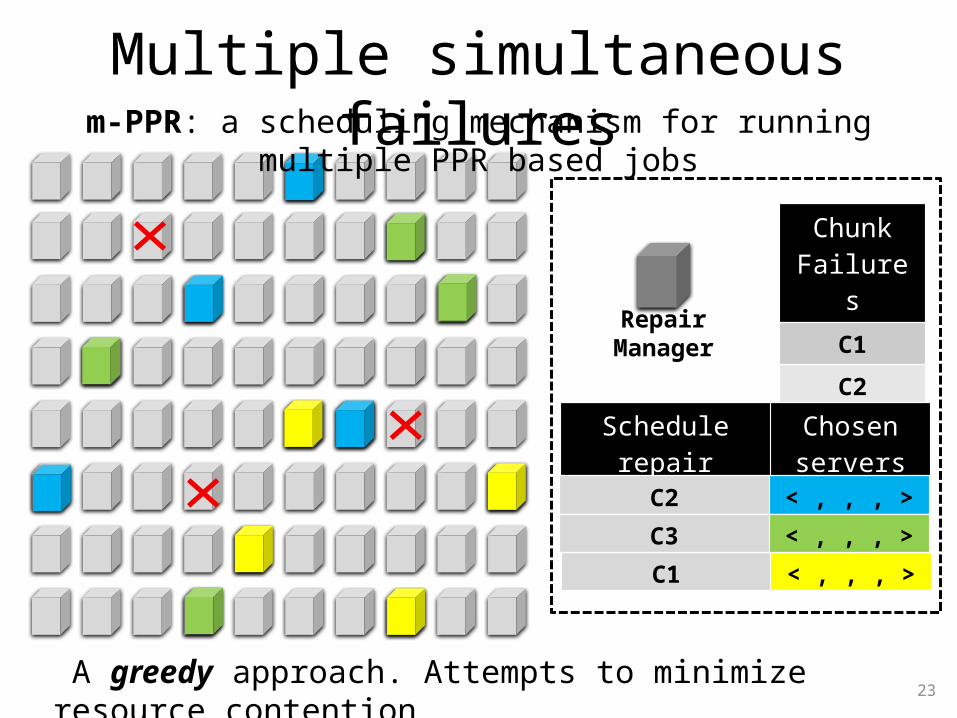
Multiple simultaneous failures

23

Chunk Failures

C1C2C3

Schedule repair Chosen servers

Repair Manager

C2 < , , , >

C1 < , , , >C3 < , , , >

m-PPR: a scheduling mechanism for running multiple PPR based jobs

A greedy approach. Attempts to minimize resource contention

24

Multiple simultaneous failures(2)

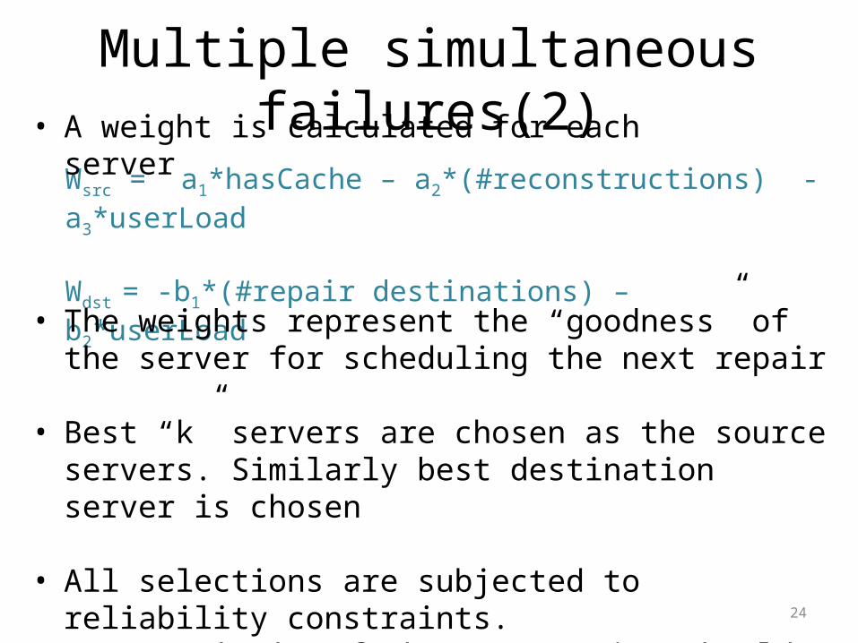
Wsrc = a1*hasCache – a2*(#reconstructions) - a3*userLoad

Wdst = -b1*(#repair destinations) – b2*userLoad

• A weight is calculated for each server

• The weights represent the “goodness” of the server for scheduling the next repair

• Best “k” servers are chosen as the source servers. Similarly best destination server is chosen

• All selections are subjected to reliability constraints. E.g. chunks of the same stripe should be in separate failure domains/update domains.

25

Implementation and evaluation

• Implemented on top of Quantcast File System (QFS) - QFS has similar architecture as HDFS.

• Repair Manager implemented inside the Meta Server of QFS

• Evaluated with various coding parameters and chunk sizes

• Evaluated PPR with Reed-Solomon code and two other repair friendly codes (LRC and Rotated-RS)

26

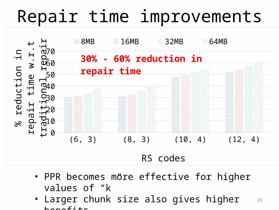
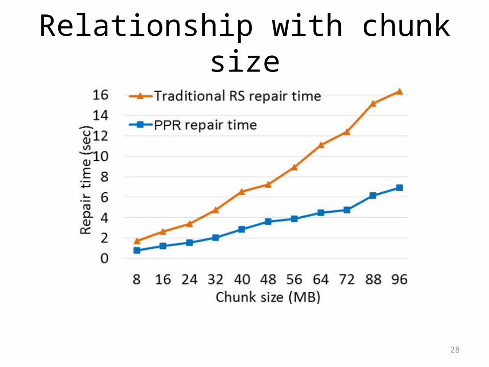
Repair time improvements

• PPR becomes more effective for higher values of “k”• Larger chunk size also gives higher benefits

(6, 3) (8, 3) (10, 4) (12, 4)0

10203040506070

8MB 16MB 32MB 64MB

RS codes

% re

ducti

on in

repa

ir tim

e w

.r.t t

radi

tiona

l rep

air

30% - 60% reduction in repair time

27

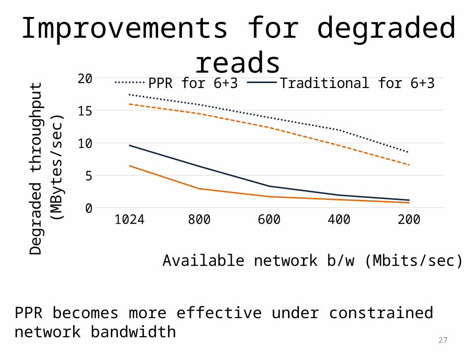
Improvements for degraded reads

PPR becomes more effective under constrained network bandwidth

1024 800 600 400 20002468

101214161820 PPR for 6+3 Traditional for 6+3

PPR for 12+4 Traditional for 12+4

Available network b/w (Mbits/sec)

Degr

aded

thro

ughp

ut

(MBy

tes/

sec)

28

Relationship with chunk size

29

Benefits from caching

30

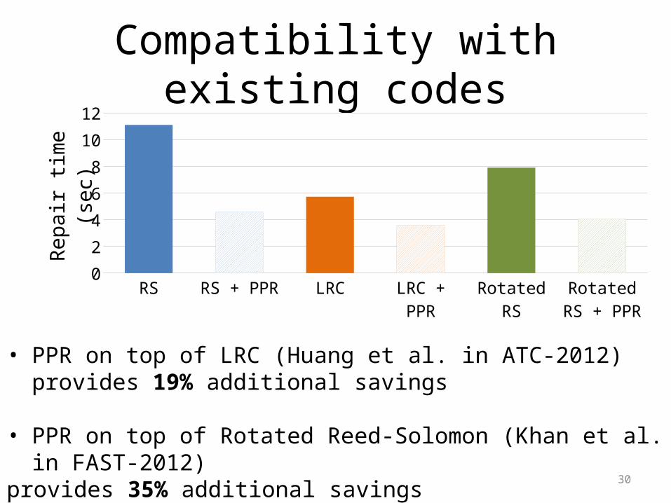
Compatibility with existing codes

• PPR on top of LRC (Huang et al. in ATC-2012) provides 19% additional savings

• PPR on top of Rotated Reed-Solomon (Khan et al. in FAST-2012)provides 35% additional savings

RS RS + PPR LRC LRC + PPR Rotated RS Rotated RS + PPR

02

4

68

1012

Repa

ir tim

e (s

ec)

31

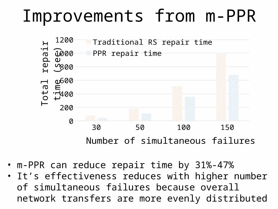
Improvements from m-PPR

30 50 100 1500

200

400

600

800

1000

1200Traditional RS repair time PPR repair time

Number of simultaneous failures

Tota

l rep

air ti

me

(sec

)

• m-PPR can reduce repair time by 31%-47%• It’s effectiveness reduces with higher number of simultaneous

failures because overall network transfers are more evenly distributed

32

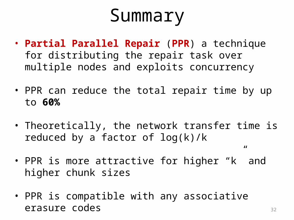
Summary• Partial Parallel Repair (PPR) a technique for distributing the

repair task over multiple nodes and exploits concurrency

• PPR can reduce the total repair time by up to 60%

• Theoretically, the network transfer time is reduced by a factor of log(k)/k

• PPR is more attractive for higher “k” and higher chunk sizes

• PPR is compatible with any associative erasure codes

33

Phase-Aware Optimization in Approximate Computing

CGO-2017

Subrata Mitra, Manish K. Gupta, Sasa Misailovic (UIUC), Saurabh Bagchi

34

Huge energy demands of computation

35

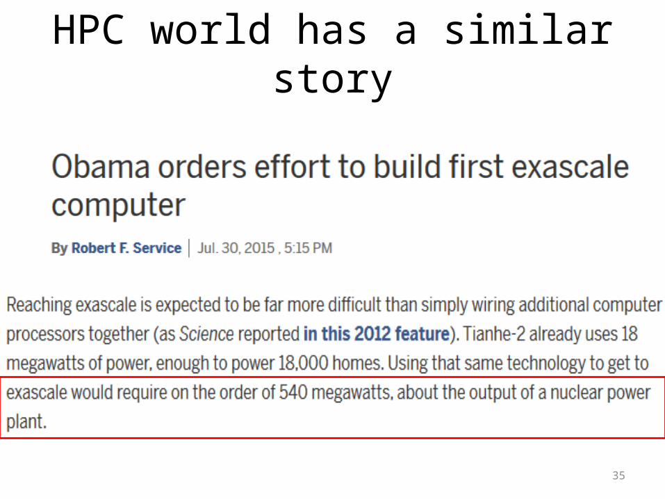
HPC world has a similar story

36

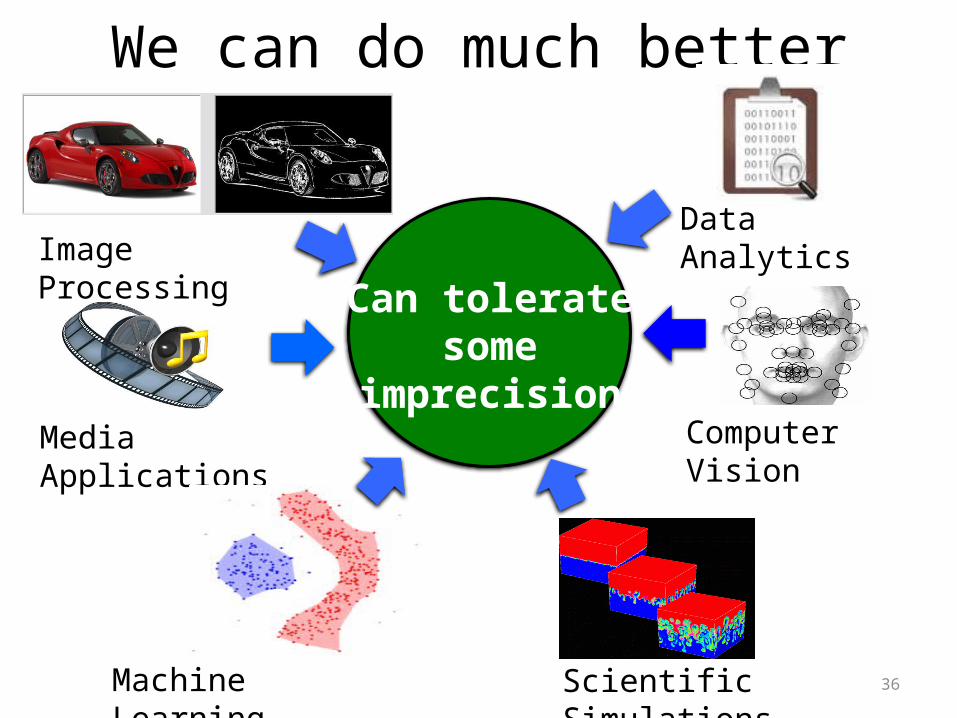
We can do much better

Can tolerate some

imprecisionComputer Vision

Data Analytics

Media Applications

Image Processing

Machine Learning Scientific Simulations

37

0% Quality Loss 5% Quality Loss 10% Quality Loss

Output quality degradation in Sobel

10% Quality loss is nearly indiscernible to the eye andyet provides 57% energy savings

Rahimi et al. DATE-2015

38

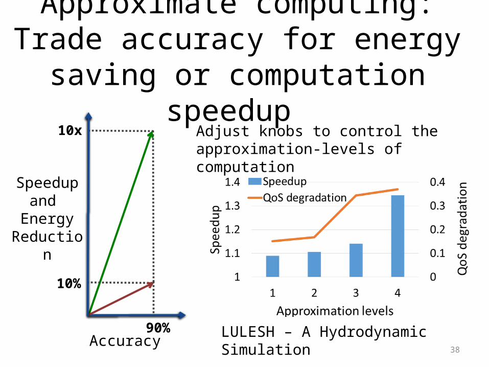
Approximate computing:Trade accuracy for energy saving or

computation speedup

Speedup and

Energy Reduction

90%

10%

10x

Accuracy LULESH – A Hydrodynamic Simulation

Adjust knobs to control the approximation-levels of computation

39

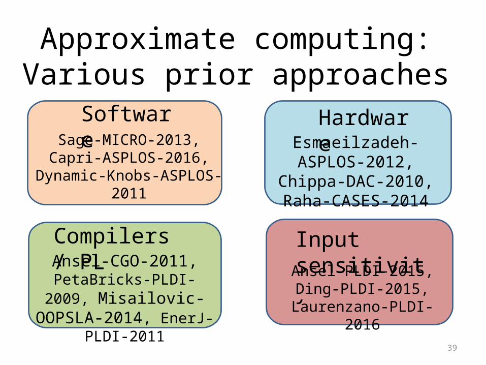
Approximate computing:Various prior approachesSoftware

Sage-MICRO-2013, Capri-ASPLOS-2016, Dynamic-Knobs-

ASPLOS-2011

HardwareEsmaeilzadeh-ASPLOS-

2012, Chippa-DAC-2010, Raha-CASES-2014

Compilers / PLAnsel-CGO-2011, PetaBricks-

PLDI-2009, Misailovic-OOPSLA-2014, EnerJ-PLDI-

2011

Input sensitivityAnsel-PLDI-2015, Ding-PLDI-

2015, Laurenzano-PLDI-2016

40

• The general approach has been to have single approximation configuration throughout the entire execution

Assumption of a monolithic execution

Output QualitySpeedup

Kernel Execution

Application Application

41

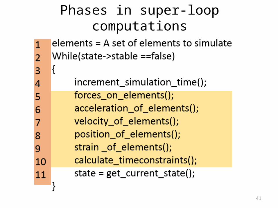
Phases in super-loop computations

42

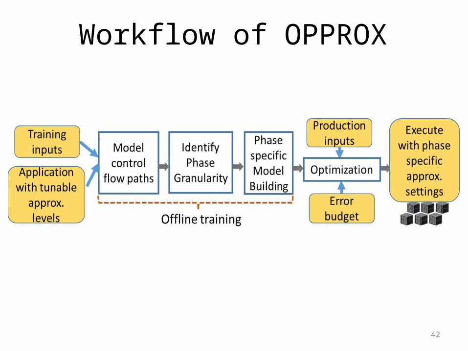
Workflow of OPPROX

43

Application with tunable approximation levels

Loop Perforation: for ( i = 0 ; i < n ; i = i + approx _level ) { result = computeresult( ) ; }Loop Truncation: for ( i = 0 ; i < ( n - approx_ level ) ; i ++) { result = computeresult( ) ; }

Loop Memoization: for ( i = 0 ; i < n ; i ++) { if (0 == i % approx_level ) cached_result = result = computeresult( ) ; else result = cached_result ; }

Parameter Tuning: Tune algorithmic controls exposed by the app.

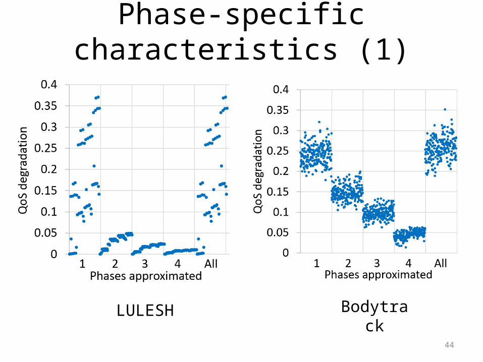
44

Phase-specific characteristics (1)

LULESH Bodytrack

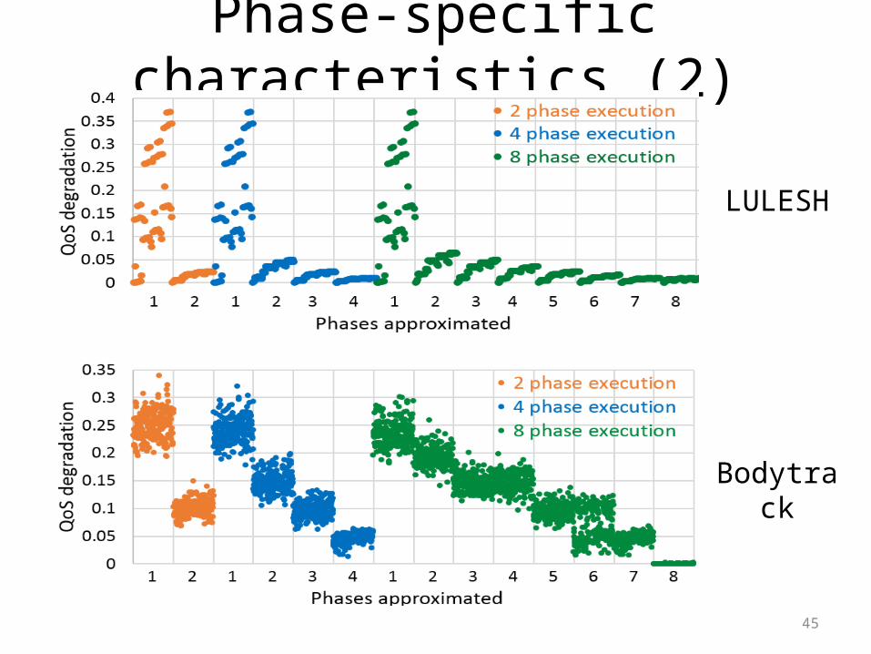
45

Phase-specific characteristics (2)

Bodytrack

LULESH

46

Choose a proper phase-granularity

< threshold

47

Application speedup

Measure speedup in terms of the number of instructions executed.

S

48

Speedup characteristics

LULESHBodytrack

49

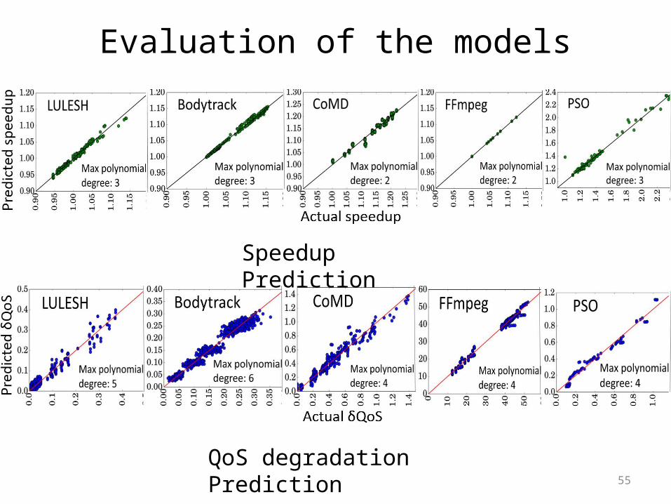
Modeling to capture phase behavior

• Collect training data for different phase-specific approximation setting.

• Build phase-specific speedup and QoS-degradation models using polynomial regression.

• For polynomial regression, the approximation knobs corresponding to different approximation blocks are the inputs and final speedup or QoS degradation are the outputs.

Example: Two approximation blocks with two knobs a1 and a2, Model for speedup with a degree-2 polynomial:

S = c0 + c1a1 + c2a2 + c3(a1)2 + c4(a2)2 + c5a1a2

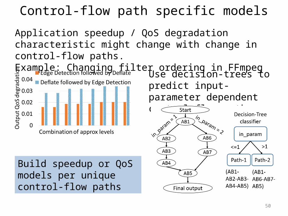
50

Control-flow path specific modelsApplication speedup / QoS degradation characteristic might change with change in control-flow paths.Example: Changing filter ordering in FFmpeg

Use decision-trees to predict input-parameter dependent control-flow paths

Build speedup or QoS models per unique control-flow paths

51

Finding phase-specific optimization• For a user provided QoS-degradation budget find the best phase-

specific optimization settings.

• First, divide the application into phases and obtain the speedup and QoS characteristics.

• Divide the error budget among the phases in proportion to their “return on investment” (mean speedup over mean error) value.

• Solve a polynomial optimization problem for each phase with the sub error budget as the constraint and find the best approximation settings for that phase.

• Redistributed any unused budget to the remaining phases.

52

Evaluations

53

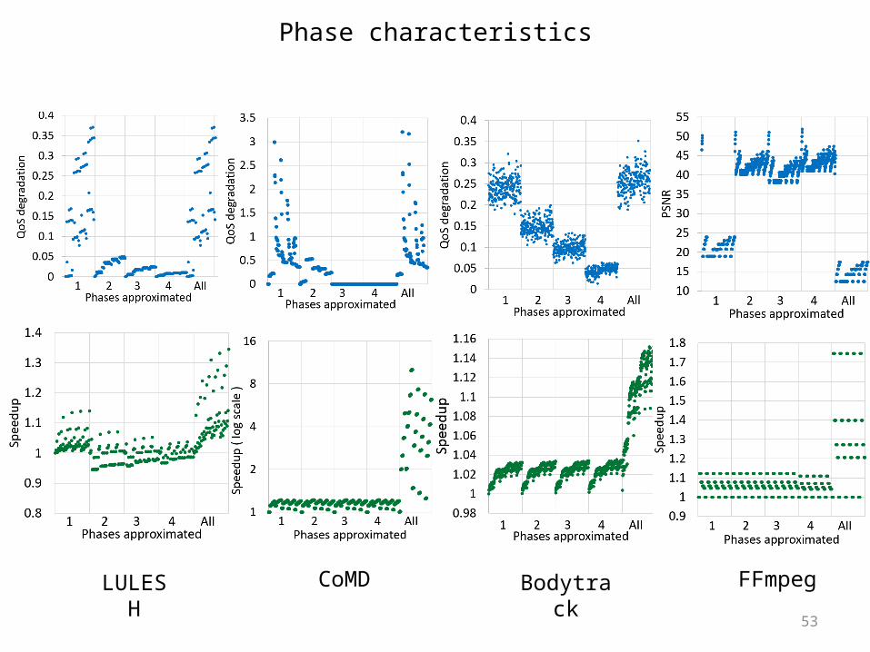
Phase characteristics

LULESH CoMD Bodytrack FFmpeg

54

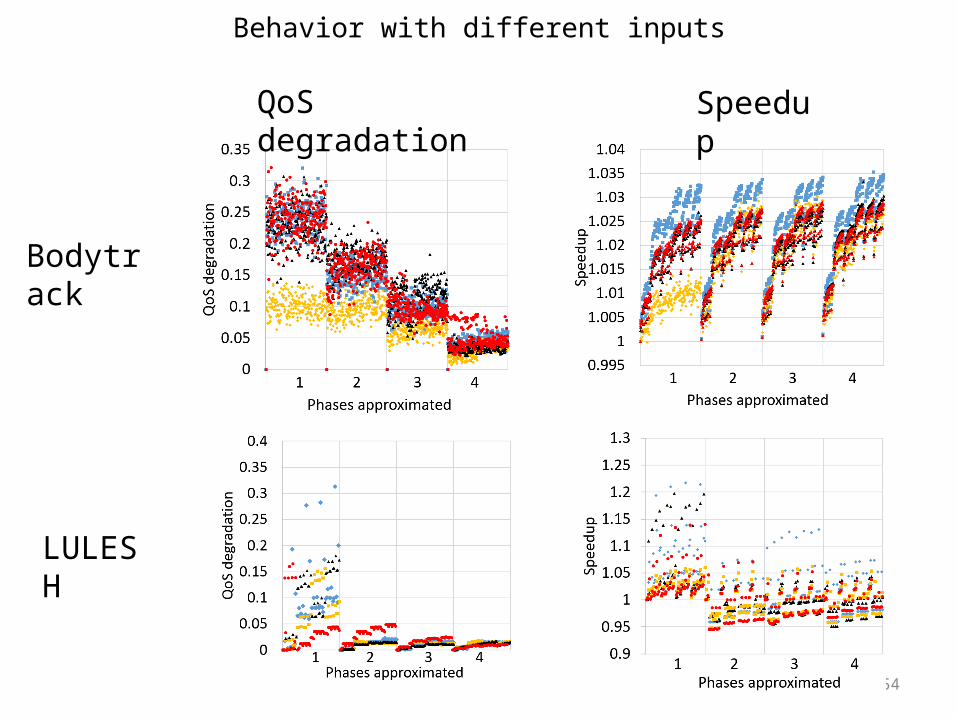
Behavior with different inputs

Bodytrack

LULESH

QoS degradation Speedup

55

Evaluation of the models

Speedup Prediction

QoS degradation Prediction

56

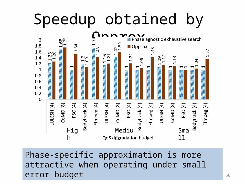
Speedup obtained by Opprox

Phase-specific approximation is more attractive when operating under small error budget

High Medium Small

57

Summary• We show when using approximation will boost application

performance, instead of “where” and “how much” we can also control “when” to fine-tune the expected outcome.

• Main computation inside a giant outer-loop which can be divided into “phases” to achieve fine-grained control over when to approximate.

• We present Opprox, a technique to characterize, model and optimize the gains from such phase-specific approximation.

• Opprox is particularly useful compared to traditional methods when operating under low error budget.

Full Papers:1. “Phase-Aware Optimization in Approximate Computing” by S. Mitra, Manish K. Gupta, S. Misailovic, S.

Bagchi, in CGO, 20172. “Partial-parallel-repair (PPR): a distributed technique for repairing erasure coded storage” by S. Mitra, R.

Panta, M-R Ra, S. Bagchi in EuroSys, 2016 3. 3“Sirius: Neural network based probabilistic assertions for detecting silent data corruption in parallel

programs” by T. Thomas, A. J. Bhattad, S. Mitra, S. Bagchi, in SRDS, 20164. “A Study of Failures in Community Clusters: The Case of Conte” by S. Mitra*, S. Javagal*, A. K. Maji, T.

Gamblin, A. Moody, S. Harrell , S. Bagchi, in IWPD@ISSRE, 20165. “Dealing with the Unknown: Resilience to Prediction Errors” by S. Mitra, G. Bronevetsky, S. Javagal, S.

Bagchi, in PACT, 20156. “VIDalizer: An Energy Efficient Video Streamer” by A. Raha*, S. Mitra*, V. Raghunathan, S. Rao in IEEE

WCNC, 20157. “ICE: An Integrated Configuration Engine for Interference Mitigation in Cloud Services” by A. Maji, S. Mitra,

S. Bagchi in ICAC, 20158. "Accurate application progress analysis for large-scale parallel debugging“ by S. Mitra, I. Laguna, D. H. Ahn,

S. Bagchi, M. Schulz, T. Gamblin in PLDI, 20149. “Mitigating Interference in Cloud Services by Middleware Reconfiguration” by A. Maji, S. Mitra, B. Zhou,

S. Bagchi and A. Verma in Middleware, 201410. "Automatic Problem Localization via Multi-dimensional Metric Profiling" by I. Laguna, S. Mitra, F.

Arshad, N. Theera-Ampornpunt, Z. Zhu, S. Bagchi, S. P. Midkiff, M. Kistler, A. Gheith in SRDS, 2013

Posters / Fast Abstracts:11. “Scalable Parallel Debugging via Loop- Aware Progress Dependence Analysis” in ‐ SC, 201312. “Cluster Workload Analytics Revisited” in DSN, 2016

List of all papers during PhD

A big thanks to all the collaborators!

Sasa (UIUC)

Greg (Google)Todd Martin

Ignacio Dong

( LLNL )

Rajesh

Moo-Ryong

( AT&T )

Suhas

Amiya

( Purdue )

And many more …

60

Backup slides

61

Sampling knob settings for training

62

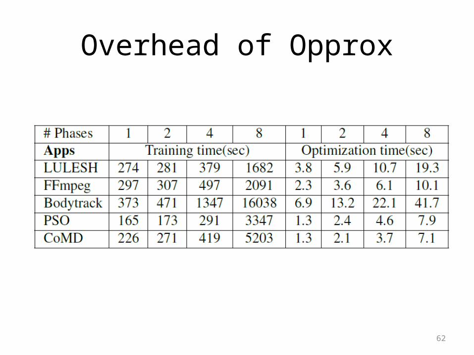
Overhead of Opprox

63

Diagnosis of performance problems at massive scale

"Accurate application progress analysis for large-scale parallel debugging"By: S. Mitra, I. Laguna, D. H. Ahn, S. Bagchi, M. Schulz, T. GamblinIn: Programming Language Design and Implementation (PLDI), 2014

64

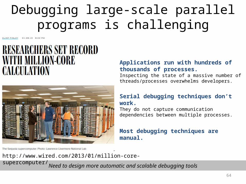
Debugging large-scale parallel programs is challenging

Applications run with hundreds of thousands of processes.Inspecting the state of a massive number of threads/processes overwhelms developers.

Serial debugging techniques don’t work.They do not capture communication dependencies between multiple processes.

Most debugging techniques are manual.

Need to design more automatic and scalable debugging tools

http://www.wired.com/2013/01/million-core-supercomputer/

65

An error in a process propagates quickly to all processes

// computation codefor (...) MPI_Send() // computation codefor (...) MPI_Recv() // computation codeMPI_Reduce()// computation codeMPI_Barrier()

Error propagation example

MPI is widely used in large-scale HPC applications.Processes communicate among them to compute the solution of a problem.

MPI processes are tightly coupled.A process needs to receive data from another process to make progress.

Error here

Some processes wait

here

All other processes wait

here

Hangs and slow execution are common bug manifestations

66

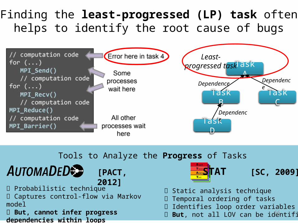
Finding the least-progressed (LP) task often helps to identify the root cause of bugs

Static analysis technique Temporal ordering of tasks Identifies loop order variables (LOV) But, not all LOV can be identified

STAT [SC, 2009]

Probabilistic technique Captures control-flow via Markov model But, cannot infer progress dependencies within loops

Tools to Analyze the Progress of Tasks

Task A

Task B Task C

Task D

DependenceDependence

Dependence

Least-progressed task

[PACT, 2012]

67

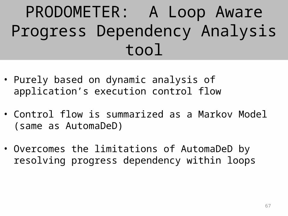
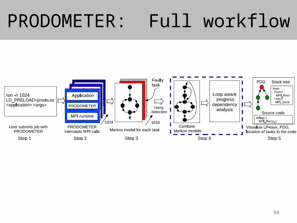
PRODOMETER: A Loop Aware Progress Dependency Analysis tool

• Purely based on dynamic analysis of application’s execution control flow

• Control flow is summarized as a Markov Model (same as AutomaDeD)

• Overcomes the limitations of AutomaDeD by resolving progress dependency within loops

68

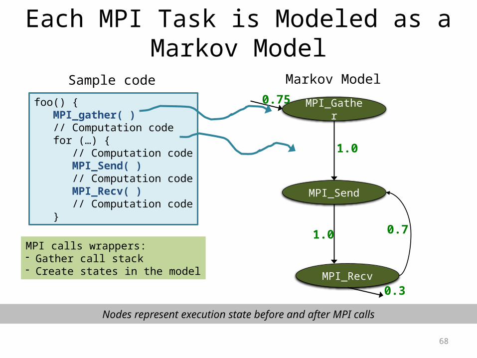
Each MPI Task is Modeled as a Markov Model

foo() { MPI_gather( ) // Computation code for (…) { // Computation code MPI_Send( ) // Computation code MPI_Recv( ) // Computation code }

Sample code

MPI_Gather

MPI_Send

MPI_Recv

1.0

1.0 0.7

0.3

0.75

Markov Model

MPI calls wrappers:- Gather call stack- Create states in the model

Nodes represent execution state before and after MPI calls

69

• The progress of the application is monitored by a helper thread

• When a hang (or slow code region) is detected, it freezes the markov model and starts the analysis phase

• Different tasks/processes wait at different nodes of the Markov model

Workflow of Prodometer

70

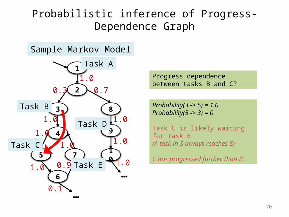
Probabilistic inference of Progress-Dependence Graph

1

2

3

4

5 7

6

8

9

10

Sample Markov Model

1.00.3 0.7

1.0

1.01.0

1.0

1.0

0.91.0

0.1

1.0…

…

Probability(3 -> 5) = 1.0Probability(5 -> 3) = 0

Task C is likely waiting for task B(A task in 3 always reaches 5)

C has progressed further than B

Progress dependence between tasks B and C?

Task C

Task D

Task A

Task B

Task E

71

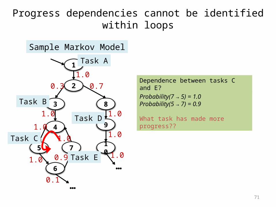
Progress dependencies cannot be identified within loops

Dependence between tasks C and E?

Probability(7 → 5) = 1.0Probability(5 → 7) = 0.9

What task has made more progress??

1

2

3

4

5 7

6

8

9

10

Sample Markov Model

1.00.3 0.7

1.0

1.01.0

1.0

1.0

0.91.0

0.1

1.0…

…

Task C

Task D

Task A

Task B

Task E

72

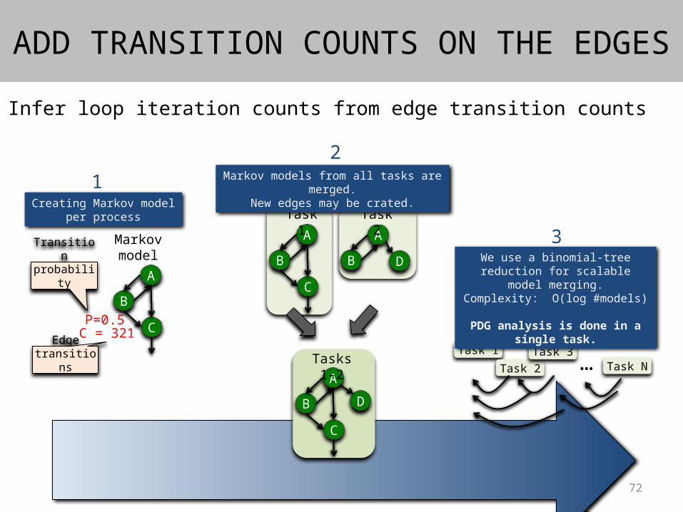
Infer loop iteration counts from edge transition counts

A

B

C

Markov model

P=0.5

Transition probability

C = 321Edge

transitions

Creating Markov model per process

A

B

C

Task 1

A

B D

Task 2

A

B

C

Tasks 1-2

D

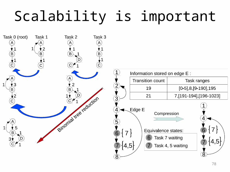
Markov models from all tasks are merged.New edges may be crated.

Task 1

Task 2Task 3

Task N…

We use a binomial-tree reduction for scalable model merging.

Complexity: O(log #models)

PDG analysis is done in a single task.

12

3

ADD TRANSITION COUNTS ON THE EDGES

73

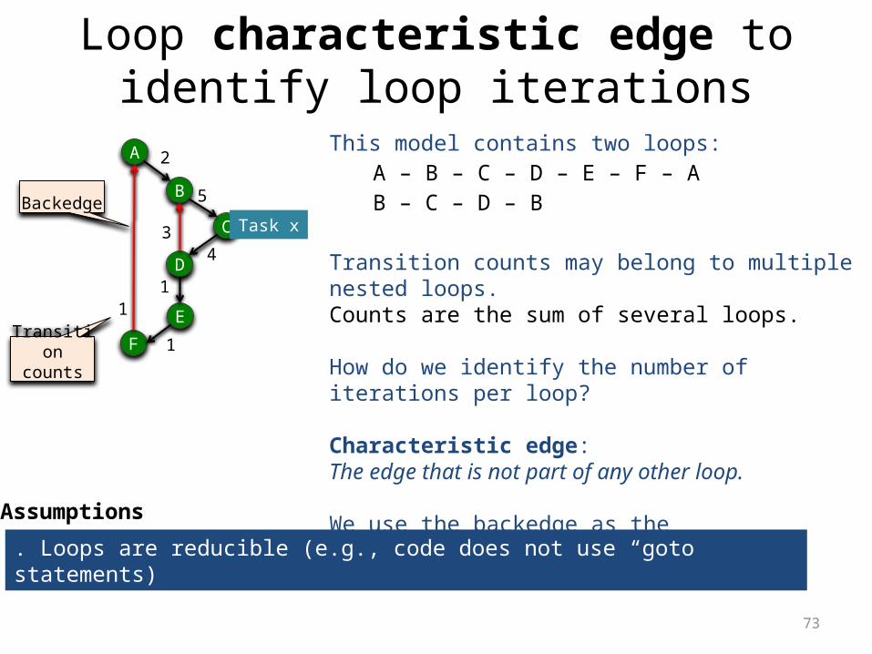
Loop characteristic edge to identify loop iterations

A

B

D

C

E

F

Task x

1

2

5

43

1

1

This model contains two loops:A – B – C – D – E – F – AB – C – D – B

Transition counts may belong to multiple nested loops.Counts are the sum of several loops.

How do we identify the number of iterations per loop?

Characteristic edge:The edge that is not part of any other loop.

We use the backedge as the characteristic edge for a loop

Transition counts

. Loops are reducible (e.g., code does not use “goto” statements)

Backedge

Assumptions

74

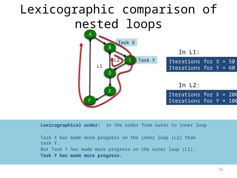
Lexicographic comparison of nested loops

Task Y

Task X

Iterations for X = 200Iterations for Y = 100

Iterations for X = 50Iterations for Y = 60

Lexicographical order: in the order from outer to inner loop

Task X has made more progress on the inner loop (L2) than task Y.But Task Y has made more progress on the outer loop (L1).Task Y has made more progress.

L1

A

B

D

C

E

F

L2

In L2:

In L1:

75

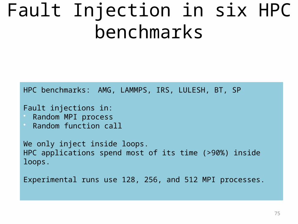
Fault Injection in six HPC benchmarks

HPC benchmarks: AMG, LAMMPS, IRS, LULESH, BT, SP

Fault injections in: Random MPI process Random function call

We only inject inside loops.HPC applications spend most of its time (>90%) inside loops.

Experimental runs use 128, 256, and 512 MPI processes.

76

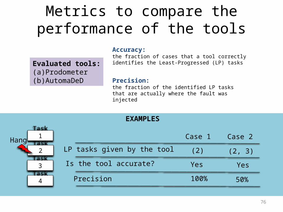
Metrics to compare the performance of the tools

Accuracy:the fraction of cases that a tool correctly identifies the Least-Progressed (LP) tasks

Precision:the fraction of the identified LP tasks that are actually where the fault was injected

Evaluated tools:(a) Prodometer(b) AutomaDeD

EXAMPLES

Task 1

Task 2

Task 3

Task 4

HangLP tasks given by the tool

Is the tool accurate?

Precision

Case 1 Case 2

(2) (2, 3)

100% 50%

Yes Yes

77

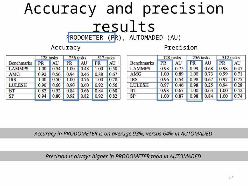
Accuracy and precision results

Accuracy

PRODOMETER (PR), AUTOMADED (AU)

Precision

Accuracy in PRODOMETER is on average 93%, versus 64% in AUTOMADED

Precision is always higher in PRODOMETER than in AUTOMADED

78

Scalability is important

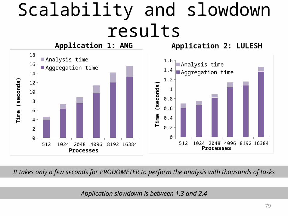
79

It takes only a few seconds for PRODOMETER to perform the analysis with thousands of tasks

Application slowdown is between 1.3 and 2.4

512 1024 2048 4096 8192 163840

2

4

6

8

10

12

14

16

18Analysis timeAggregation time

Processes

Tim

e (s

econ

ds)

512 1024 2048 4096 8192 163840

0.2

0.4

0.6

0.8

1

1.2

1.4

1.6Analysis timeAggregation time

ProcessesTi

me

(sec

onds

)

Application 1: AMG Application 2: LULESH

Scalability and slowdown results

80

PRODOMETER: Full workflow

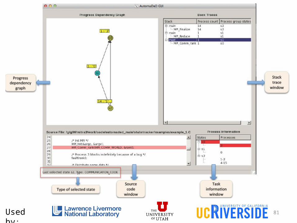
81Used by:

82

Input aware performance anomaly detection

“Dealing with the Unknown: Resilience to Prediction Errors” By: S. Mitra, G. Bronevetsky, S. Javagal, S. BagchiSubmitted to: PACT 2015

83

Complex software have too many factors influencing its performance

• Factors = configuration parameters, execution environment, input data

• Not possible to test all the combinations

• When performance degrades, hard to understand whether it was expected or something went wrong

84

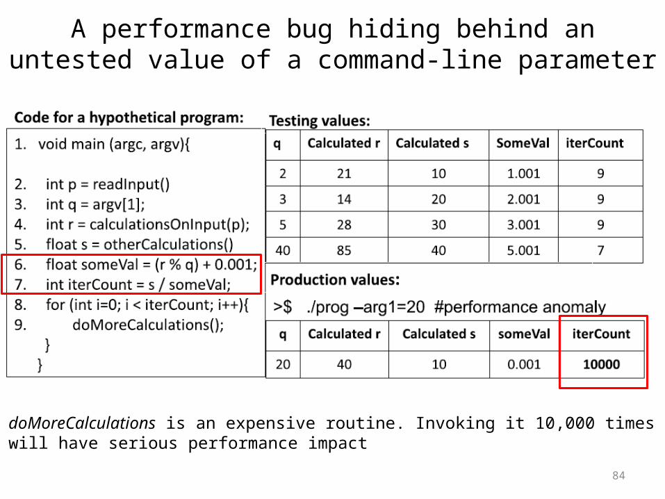
A performance bug hiding behind an untested value of a command-line parameter

doMoreCalculations is an expensive routine. Invoking it 10,000 times will have serious performance impact

85

Statistical models are often created to predicted the performance of an application. But ...

• Many configuration parameters, each taking a range of values – almost impossible to cover all combinations

• Performance changes with size of the input• Performance changes with characteristics of the input

- density of a graph- sparsity of a matrix

• Often model is created with limited training runs. Parameters/inputs used in production are drastically different

Errors in performance prediction models must be characterized

86

Systematic characterization of prediction errors are useful in many scenarios

• Scheduler might consider it while predicting execution time and resource usage

• In approximate computing, such error characteristics might guide the decision of replacing actual code regions by prediction models for speed up and reduced energy consumption

• An anomaly detection tool may use it when distinguishing normal behavior from anomalous behavior to reduce false alarms

87

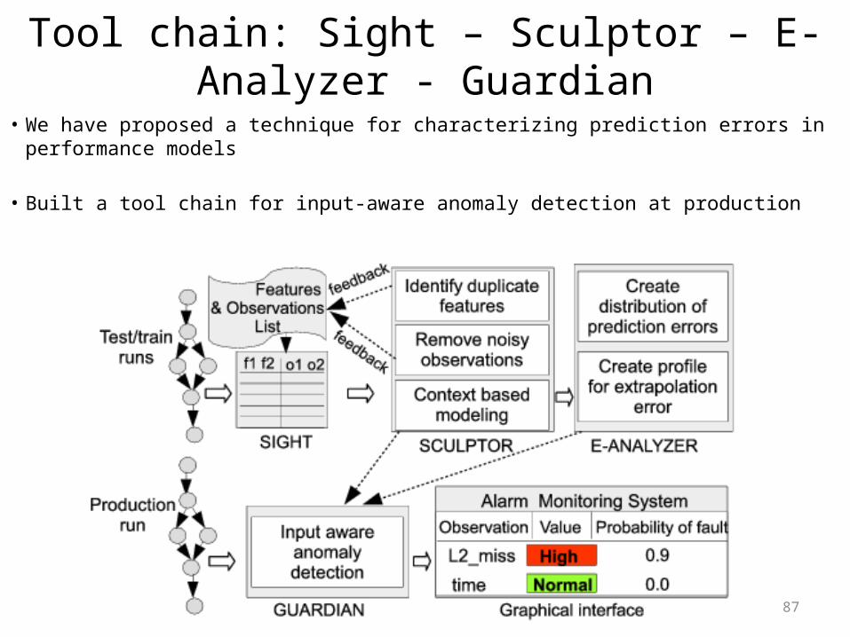
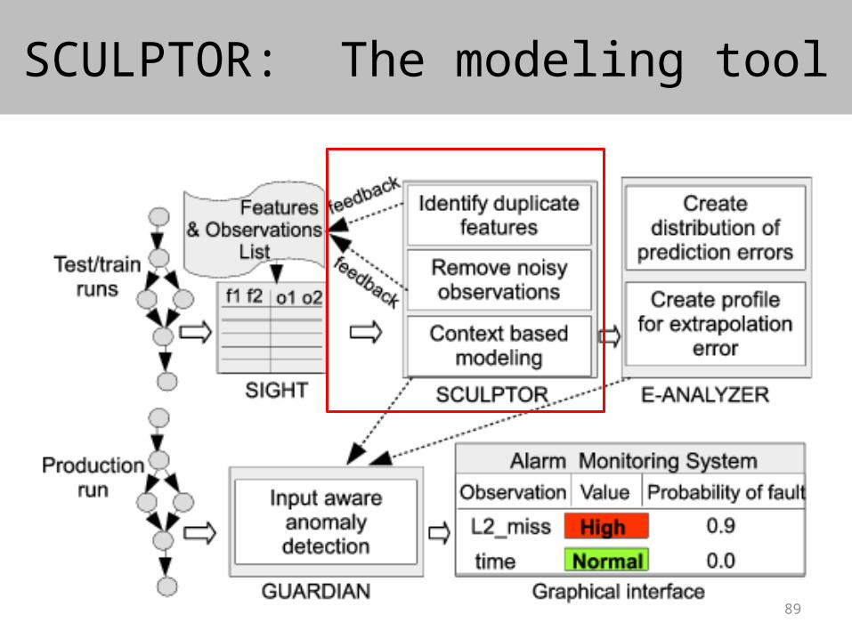
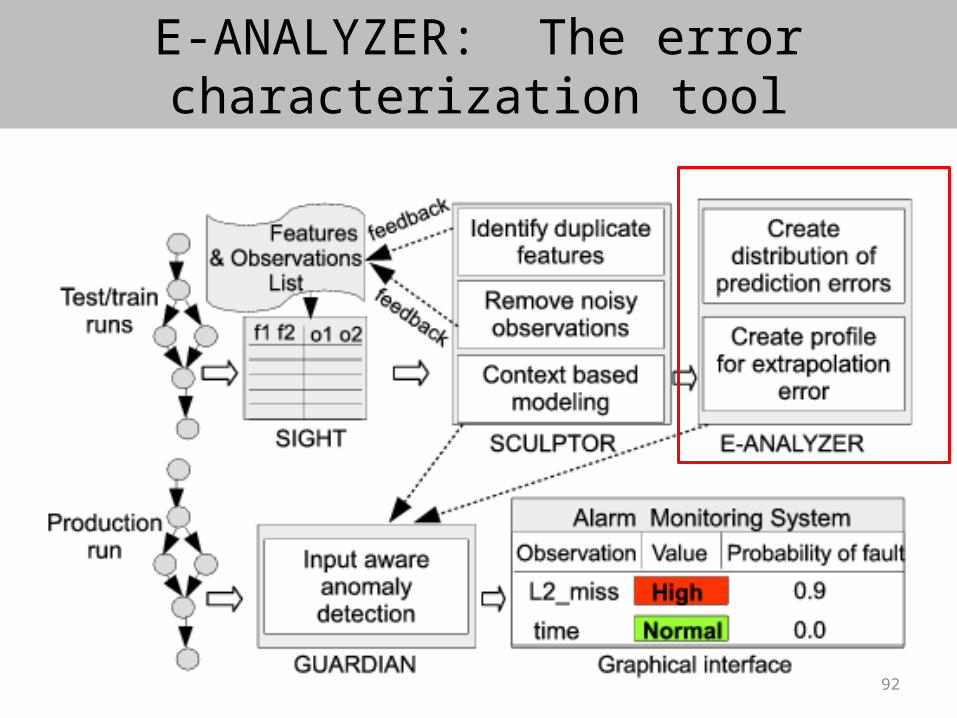
Tool chain: Sight – Sculptor – E-Analyzer - Guardian• We have proposed a technique for characterizing prediction errors in performance

models

• Built a tool chain for input-aware anomaly detection at production

88

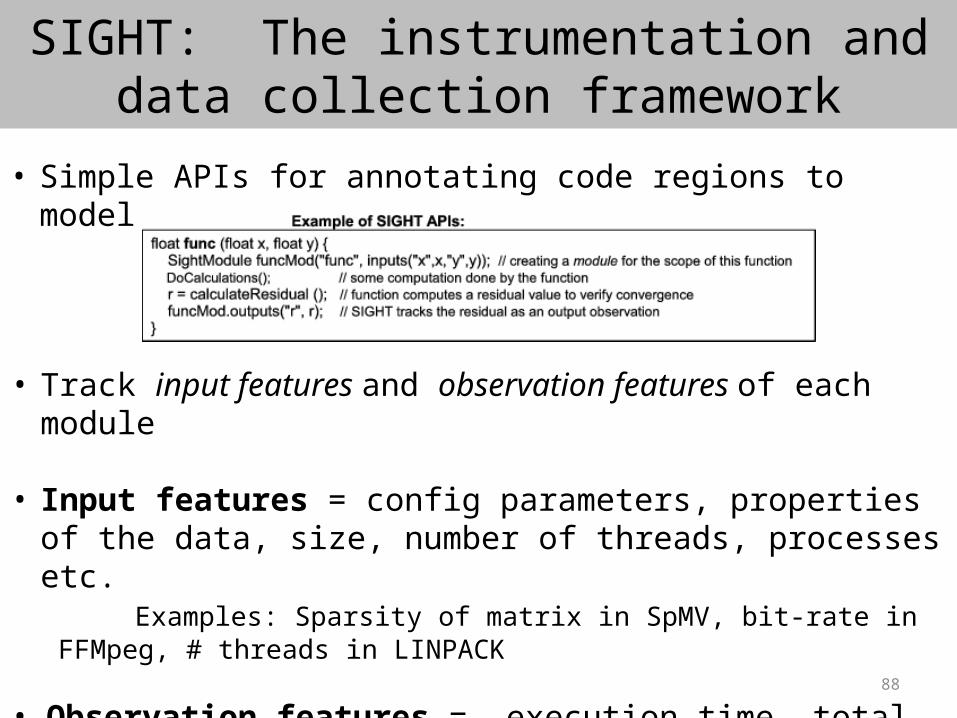
SIGHT: The instrumentation and data collection framework

• Simple APIs for annotating code regions to model

• Track input features and observation features of each module

• Input features = config parameters, properties of the data, size, number of threads, processes etc.

Examples: Sparsity of matrix in SpMV, bit-rate in FFMpeg, # threads in LINPACK

• Observation features = execution time, total number of instructions, load instructions, cache miss rate, residue value etc.

89

SCULPTOR: The modeling tool

90

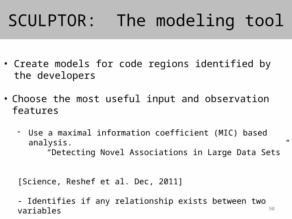
SCULPTOR: The modeling tool

• Create models for code regions identified by the developers

• Choose the most useful input and observation features

- Use a maximal information coefficient (MIC) based analysis. “Detecting Novel Associations in Large Data Sets” [Science, Reshef et al. Dec, 2011]

- Identifies if any relationship exists between two variables

- Works even for non-linear relationships

• Model using polynomial regression up to degree 3

91

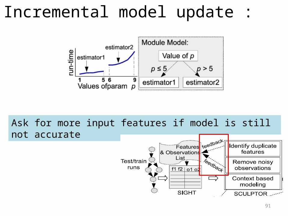
Incremental model update :

Ask for more input features if model is still not accurate

92

E-ANALYZER: The error characterization tool

93

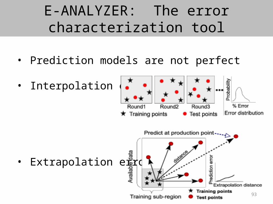
E-ANALYZER: The error characterization tool

• Prediction models are not perfect

• Interpolation error

• Extrapolation error

94

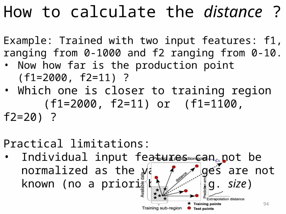
How to calculate the distance ?

Example: Trained with two input features: f1, ranging from 0-1000 and f2 ranging from 0-10. • Now how far is the production point (f1=2000, f2=11) ?• Which one is closer to training region (f1=2000, f2=11) or (f1=1100, f2=20) ?

Practical limitations:• Individual input features can not be normalized as the

valid ranges are not known (no a priori bound: e.g. size)

95

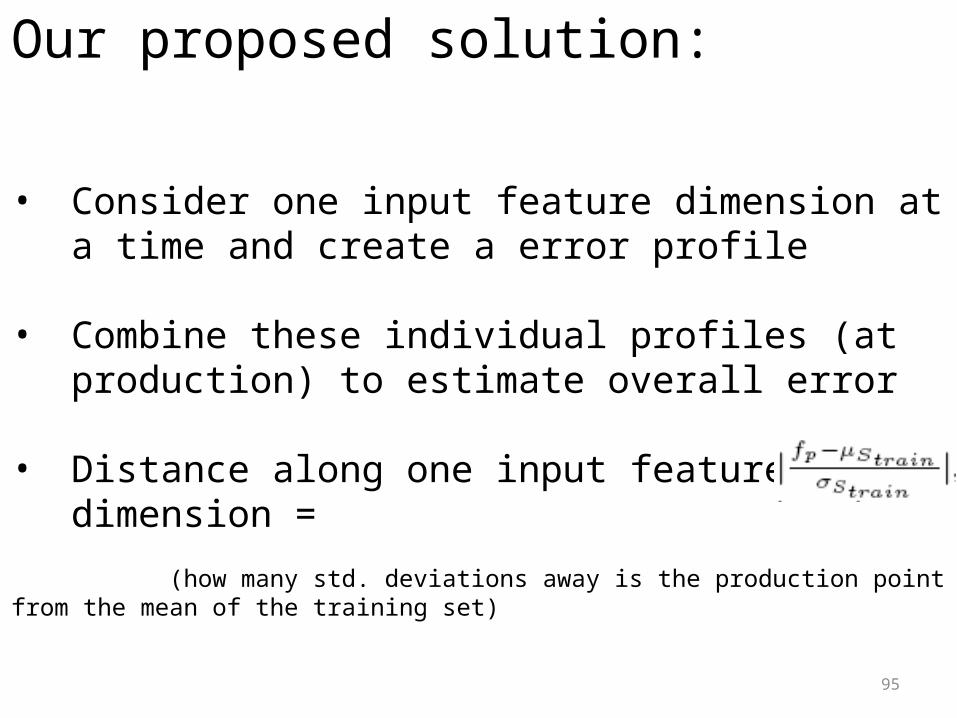
Our proposed solution:

• Consider one input feature dimension at a time and create a error profile

• Combine these individual profiles (at production) to estimate overall error

• Distance along one input feature dimension = (how many std. deviations away is the production point from the mean of the training set)

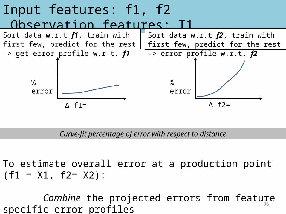
96

Input features: f1, f2 Observation features: T1

% error

Δ f1=

% error

Sort data w.r.t f1, train with first few, predict for the rest -> get error profile w.r.t. f1

Sort data w.r.t f2, train with first few, predict for the rest -> error profile w.r.t. f2

To estimate overall error at a production point (f1 = X1, f2= X2):

Combine the projected errors from feature specific error profiles

Δ f2=

Curve-fit percentage of error with respect to distance

97

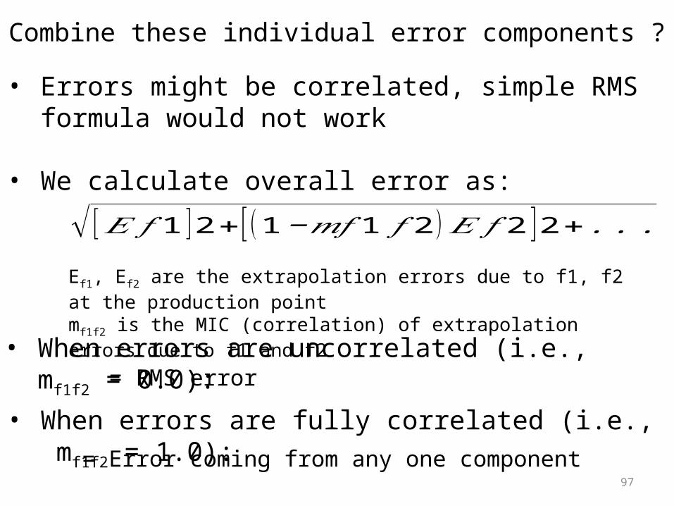
Combine these individual error components ?

• Errors might be correlated, simple RMS formula would not work

• We calculate overall error as:

√ [𝐸 𝑓 1 ] 2+ [ (1−𝑚𝑓 1 𝑓 2 ) 𝐸 𝑓 2 ]2+ .. .

Ef1, Ef2 are the extrapolation errors due to f1, f2 at the production pointmf1f2 is the MIC (correlation) of extrapolation errors due to f1 and f2

• When errors are uncorrelated (i.e., mf1f2 = 0.0):

• When errors are fully correlated (i.e., mf1f2 = 1.0):

= RMS error

= Error coming from any one component

98

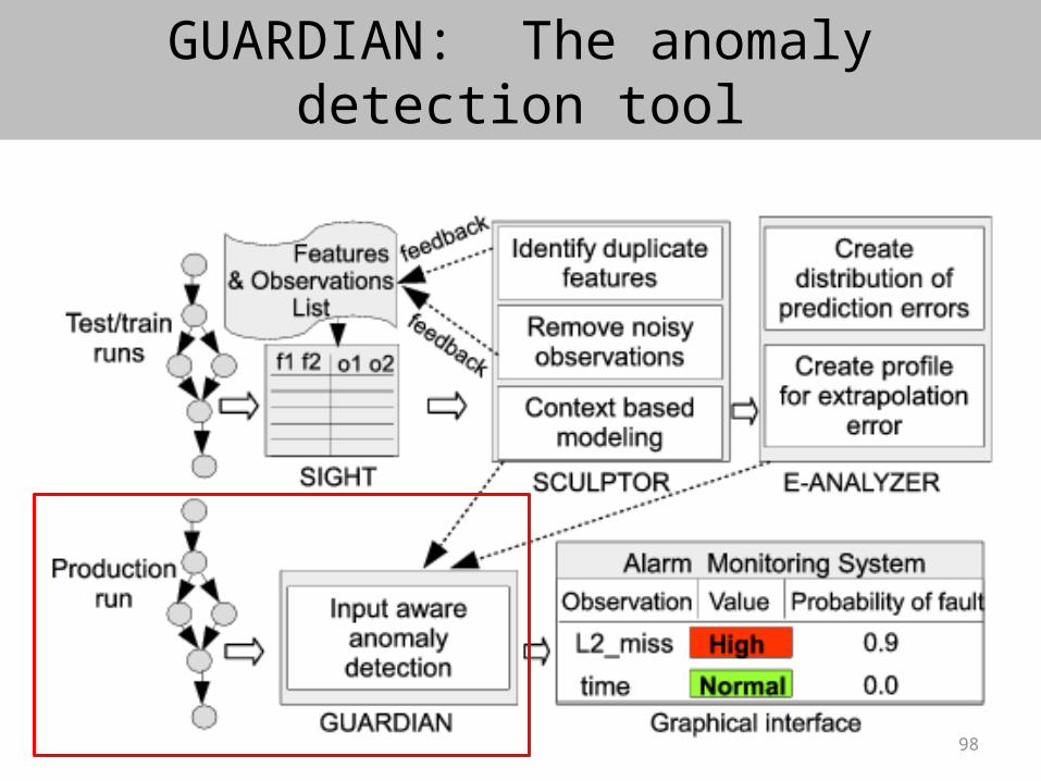
GUARDIAN: The anomaly detection tool

99

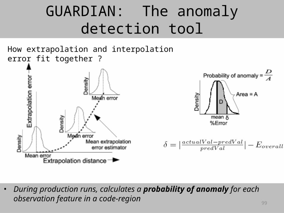
GUARDIAN: The anomaly detection tool

• During production runs, calculates a probability of anomaly for each observation feature in a code-region

How extrapolation and interpolation error fit together ?

100

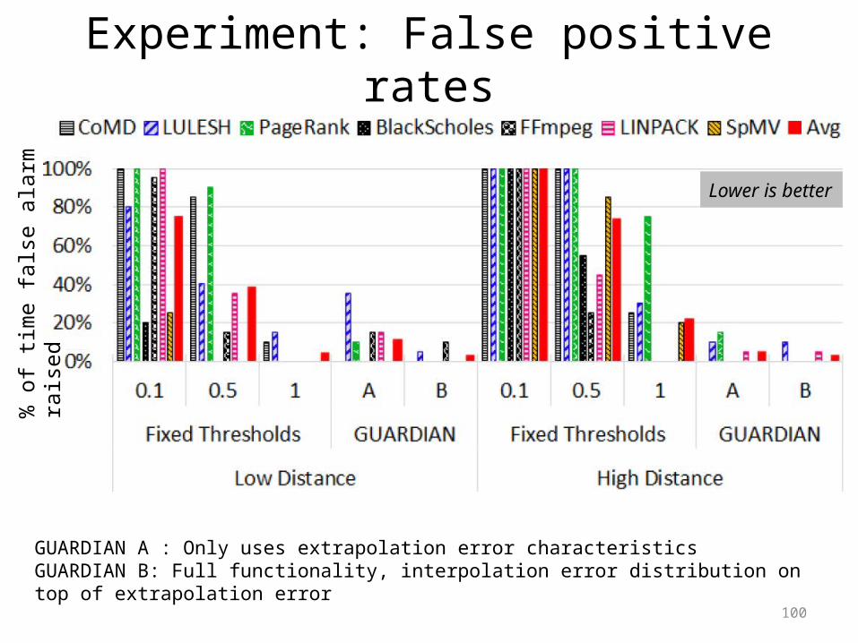
Experiment: False positive rates

Lower is better

% o

f tim

e fa

lse a

larm

raise

d

GUARDIAN A : Only uses extrapolation error characteristicsGUARDIAN B: Full functionality, interpolation error distribution on top of extrapolation error

101

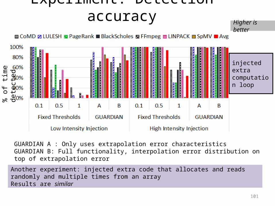
Experiment: Detection accuracyHigher is better

injected extra computation loop

Another experiment: injected extra code that allocates and reads randomly and multiple times from an arrayResults are similar

GUARDIAN A : Only uses extrapolation error characteristicsGUARDIAN B: Full functionality, interpolation error distribution on top of extrapolation error

% o

f tim

e de

tect

ed