WG-KRll.L-92/11

STATUS OF KRILLTARGET STRENGTH

K.G. Foote1, D. Chu2 and T.K. Stanton2

Abstract

Empirical estimates for the target strength of krill are extracted from publications. These are confined to measurements on aggregations of live euphausiids and should not be affected by a frequent cause of bias in single-animal measurements, namely thresholding. Theoretical estimates for the target strength are derived from the deformed-cylinder scattering model assuming specific sets of physical and orientational parameters, for which there is an empirical basis. The theoretical estimates show a non-monotonic dependence of target strength on both animal size and transmit frequency, notwithstanding admitted shortcomings. Some recent single-animal measurements of target strength for live euphausiids and euphausiid-related species, made under high signal-to-noise-ratio conditions, are consistent with the general pattern. Several specific recommendations are made for future, improved determinations of krill target strength. Based on the comparisons, general prediction curves for the target strength are presented that are applicable to a wide range of lengths, acoustic frequencies and orientation parameters.

Resume

Les estimations empiriques de la reponse acoustique du krill sont extraites des publications. Elles sont limitees aux mesures des concentrations d'euphausiaces vivants et ne devraient pas etre affectees par une cause frequente de biais dans les mesures des individus, a savoir l'identification du seuil. Les estimations theoriques de la reponse acoustique sont derivees du modele de diffusion en cylindre deforme, presumant des series specifiques de parametres physiques et d'orientation reposant sur une base empirique. Les estimations tMoriques mettent en evidence une dependance non monotone entre la reponse acoustique et a la fois la taille des individus et la frequence de transmission, en depit des limites admises. Quelques mesures de reponse acoustique prises recemment sur des individus vivants (un par un) d'especes d'euphausiaces et d'especes apparentees aux euphausiaces, effectuees dans des conditions dans lesquelles le rapport signal-bruit est elevee, suivent le modele general. Plusieurs recommandations specifiques sont avancees pour une meilleure determination de la reponse acoustique du krill a l'avenir. Basees sur les comparaisons, les courbes generales de prediction de la reponse acoustique presentees sont applicables a tout un eventail de longueurs, de frequences acoustiques et de parametres d'orientation.

1 Institute of Marine Research, PO Box 1870, N 5024 Bergen, Norway 2 Woods Hole Oceanographic Institution, Woods Holes, MA, USA

101

Pe3lOMe

3Mnl1pH4eCKHe Ol\eHKH CHJIbI l\eJIH KPHJI5I 6bIJIH B35ITbI H3

Pa.3JIH4HbIX ny6JIHKal\HH. OHH KaCaIOTC5I TOJIbKO H3MepeHHH

npOBe,lleHHbIX Ha CKOnJIeHH5IX )l{HBbIX 3B<PaY3HH,ll H Ha HHX He

,llOJI)I{eH OK a.3 bIB a Tb BJIH5IHHe "noporOBOH 3<p<peKT", KOTOPbIH

4aCTO BbI3bIBaeT cMellleHHe H3MepeHHH, npOBe,lleHHbIX Ha

e,llHHH4HhlX )l{HBOTHhlX. TeopeTH4eCKHe Ol\eHKH CHJIhl l\eJIH

nOJIY4eHbI C nOMOlllblO MO,lleJIH pacceHBaHH5I ,lle<popMHpO­

BaHHbIM l\HJIHH,llPOM, npe,llnOJIaraJIH HaJIH4He KOHKpeTHbIX

Ha6opOB <pH3H4eCKHX H opeHHTal\HOHHbIX napaMeTpOB, ,llJI5I

KOTOPbIX HMeeTC5I 3MnHpH4eCKoe 060CHOBaHHe. HecMoTp5I Ha

HMelOlllHeC5I B paC4eTax He,llOCTaTKH, TeopeTH4eCKHe Ol\eHKH

YKa.3bIBaIOT Ha OTCYTCTBHe MOHOTOHH4eCKOH 3aBHCHMOCTH

CHJIbI l\eJIH KaK OT pa.3Mepa )l{HBOTHOro, TaK H OT 4aCTOTbI

nepe,llaT4HKa. HeCKOJIbKO npOBe,lleHHhlX He,llaBHO H3MepeHHH

CHJIbI l\eJIH )l{HBbIX 3B<PaY3HH,ll H 6JIH3KHX K HHM BH,llOB,

npO,lleJIaHHbIX B YCJIOBH5IX BbICOKoro COOTHOrneHH5I CHrHaJIa K

rnyMy, COOTBeTCTBYIOT o6111eH KapTHHe. IIpHBO,llHTC5I p5I,ll

KOHKpeTHbIX peKOMeH,llal\HH no YJIY4rneHHlO onpe,lleJIeHH5I

CHJIbI l\eJIH KPHJI5I B 6Y,llYllleM. Ha OCHOBe cpaBHeHHH, ,llaIOTC5I

o6111He nporHo3HpyeMble KpHBble CHJIbI l\eJIH, npHMeH5IeMbIe K

rnHpoKoMY ,llHana.30HY ,llJIHH, aKycTH4ecKHx 4aCTOT H

0pHeHTal\HOHHbIX n apaMeTpoB.

Resumen

Los valores empfricos de la potencia del blanco del kri! han sido extrafdos de las publicaciones. Estos se limitan a mediciones hechas en cardumenes de eufausidos libres y no debieran ser afectados por una fuente de desviacion frecuente experimentada en las mediciones de animales individuales, es decir, por la formacion de umbrales. Los valores teoricos de la potencia del blanco son deducidos del modelo de dispersion del cilindro deforrnado, suponiendose una serie especffica de variables ffsicas y orientacionales para las cuales existe una base empfrica. Los valores teoricos muestran una dependencia no-monotona de la potencia del blanco con respecto al tamafio del animal y a su frecuencia de transmision, a pesar de las reconocidas limitaciones. Algunas mediciones recientes de potencia del blanco en eufausidos vivos y en especies afines, hechas en condiciones de alta relacion seiial/ruido, son consecuentes con el modelo general. Se formulan varias recomendaciones especfficas para mejorar las futuras estimaciones de potencia del blanco del kril. Sobre la base de las comparaciones, se presentan las curvas de prediccion general para la potencia del blanco que son aplicables a una amplia gama de tallas, frecuencias acusticas y parametros orientacionales.

1. INTRODUCTION

The echo integration method (Forbes and Nakken, 1972; MacLennan, 1990) has been applied to krill (Euphausia superba) in the Southern Ocean (Miller and Hampton, 1989). In order to convert measurements of echo strength to biological quantities, such as the number density of scatterers, knowledge of target strength is essential. Notwithstanding the degree of

102

! :/

interest in krill biomass, as witnessed, for example, by the scale of international involvement in the Biological Investigation of Marine Antarctic Systems and Stocks (BIOMASS) program, measurements of kriU target strength have been quite scarce.

In fact, at the time of the Post-FIBEX Acoustic Workshop in 1984 (Anon., 1986) only several measurements on E. superba had been reported in the literature. In order to establish a target strength-size relationship for use in interpreting the measurements of the First International BIOMASS Experiment (FIB EX), recourse was made to measurements on other zooplankton. These included measurements on preserved, defrosted and even live specimens of other species. In many cases, the measurements were performed on single specimens. It is the authors' contention that such measurements, while being inherently difficult for weak, zooplankton scatterers, are vulnerable to the effect of thresholding.

Thresholding, or the discarding or rejection of signals as noise because of their low amplitude, low spectral level, or other inferior characteristics, has been recognised as an important phenomenon in fish-scattering measurements (Weimer and Ehrenberg, 1975; Foote et al., 1986). Its recognition in zooplankton acoustics has been less common. Clearly its mention in the literature as a possible source of bias in single-scatterer measurement has been rare. The kind of review attempted here may consequently be justified for gathering together diverse, generally recent references on scattering by live euphausiids that avoid or otherwise address the effect of thresholding.

The organisation of this paper is the following. The quantities of target strength, back scattering cross section, and mean volume backscattering coefficient and strength are defined. Empirical studies of krill target strength, based on measurements of the mean volume back scattering strength are summarised, and a theoretical model for krill scattering is described. Both measurements and theory are combined. On this basis, target strength-size relationships are proposed for current use in acoustic surveys of krill aggregations or stocks. In addition to considering both the presented measurements and theoretical computations, comparisons are made with data involving individuals, and recommendations are made for improving the determination of krill target strength.

2. DEFINmONS

Target strength gives a measure of backscattering or echo strength intrinsic to the scatterer itself. It is useful sometimes to keep in mind its origin in basic scattering physics. A plane, harmonic wave is assumed to be incident on an isolated, finite body in a homogeneous fluid medium. In terms of pressure,

Pine = A exp [i(k· r - rot)],

where A is the amplitude, k is the wave vector, r is the position where the incident pressure field is to be evaluated, (0 is the angular frequency, and t is time. The scattered pressure field in the far-field of the body is typically expressed in terms of the spherical wave exp(ikr)/r. Suppressing the time dependence exp( -i(O t),

Um

r~oo p = Afexp(ikr)/r, se

where fis the far-field scattering amplitude. The backscattering cross section, 0' or O'bs, is defined in terms of the far-field backscattering amplitude fb thus:

(1)

103

The quantity C1bs is also called the differential scattering cross section in the backscattering direction. Because of the frequently large range in values of C1 or C1bs for the same or similar scatterers, a logarithmic measure is convenient. This is the target strength TS,

0' TS = 10 log - = 10 log O'bs'

41l' (2)

where the backscattering cross section is expressed in SI units. The TS of an idealised, perfectly reflecting sphere of 2 m radius at very high frequency is 0 dB.

Theoretical and empirical studies show that it is sometimes useful to normalise the back scattering cross section by the square of the length of the body, provided of course that the body is elongated. In this paper, krilllength refers consistently to the distance from the anterior end of the eye to the tip of the telson. When the length is not defined in the cited data source, it is assumed to be tantamount to this. Expression of the normalised cross section in the logarithmic domain results in the reduced target strength,

(3)

It is convenient to represent RTS as a function of the equivalent cylindrical radius a of the body, normalised by the multiplicative factor k. The advantage of presenting RTS versus ka is that data spanning a wide range of lengths and frequencies can be compared on the same plot. The present definitions of C1, C1bs, TS, and RTS apply strictly to harmonic waves. Although useful as a concept, such continuous waves are fictional. A backscattering cross section or target strength can also be defined for finite-duration waves or signals (Foote, 1982). However, the continuous-wave or harmonic-wave approximation is excellent for the several data sources considered in the next section. This is due to the fact that the distance spanned by a ping is much larger than any dimension of the animals.

The above definitions also pertain only to single realisations of the scattering from individuals. Accordingly, the state of an animal is defined by a unique combination of orientation, body shape including bend, taper and roughness, and physical properties. Adding to the complexity of the description of the scattering are the facts that (1) echoes from individual krill tend to fluctuate from ping to ping as the animals change shape and orientation, and (2) echoes from animals that are not acoustically resolved or separated, because of overlap with echoes from other animals, also tend to fluctuate from ping to ping because of the stochastic nature of the interference between the echoes from each animal. In order to describe the scattering involving the fluctuating echoes, the following averages of the above quantities are defined:

Data

(4)

Theory

a(L) = feO'(L,8)fe(8)d8 (individual), (5)

o = fL o(L )fL (L)dL (aggregation), (6)

104

The definitions are divided into two broad categories. Equation (4) represents the measured backscattering cross section averaged over N pings. This equation could be applied to repeated observations of the same individual or many observations of different individuals. Thus the average might involve, for example, behaviour through the tilt angle e, or both behaviour and length through e and L, respectively. Equations (5) and (6) are the respective theoretical counterparts, where Ix denotes the appropriate probability density function of variable X. Equation (5) is typically more appropriate for use in the laboratory where animals are studied on an individual basis, while equation (6) is more applicable in the field where an aggregation of animals over a range of lengths will typically exist. The above averages apply to both 0' and O'bs. All averages involve the addition of energies (cross sections) because the energy is most appropriate for describing the incoherent addition of echoes from animals in aggregations. Finally, the above theoretical averages are shown with just a few variables over which the averages are made. Generalisations are possible for inclusion of other effects, such as the degree of bend or flexure of the animal, as represented by its radius of curvature, or the degree of roughness of the body.

The "average" target strength can be defined in terms of the average backscattering cross section as

TS = 10 log (J' / 4n) = 10 logO" bs' (7)

where the averaging is performed before the logarithm is taken. The average reduced target strength is defined in a similar manner.

The mean volume backscattering coefficient Sv is related to the mean backscattering cross section and the number density p of scatterers (Stanton et al., 1987),

0" -Sv = p- = pO" 4n bs'

(8)

where the usual convention of not indicating the average nature of Sv by an overhead bar is used. This quantity can be determined through the sonar equation (Urick, 1975), given knowledge of the transmit and receive conditions, including beam pattern characteristics. In the logarithmic domain,

Sv = 10 log P + TS (9)

where Sv is the mean volume backscattering strength. This or similar volume scattering quantities are typically what are measured in the field, especially when the animals are not resolved by the sonar. Relating raw echo levels to Sv requires knowledge of sonar system parameters such as ping duration and beam pattern. Single animal target strengths can only be measured directly when the echoes from the different animals are not overlapping.

3. EMPIRICAL VALUES OF TARGET SlRENGTH

Estimating the target strength of zooplankton is far from straightforward because of the behaviour of the animals and thresholding of the sonar system. When the animal is insonified at or near broadside incidence, the resultant echo is strong and the sonar will be most able to record it. However, at or near end-on incidence, the echo is quite weak. When measuring target strengths of (resolved) individuals in the laboratory or field, the echoes from end-on incidence may be below the noise level or "detection threshold" of the sonar, hence the echo goes unrecorded. The average from measurements of individuals will involve only the average of values above the threshold, causing an overestimate (threshold bias) of target strength. In the other case, when the animals are measured collectively, i.e., when the animals are not resolved by

105

the sonar, the echoes from some animals may be above the threshold while those from others may not. The resultant echo from this aggregation is detectable and an average target strength is determined by normalising the echo level (or energy) by the total number of animals regardless of whether all of them would have been detectable individually. The threshold bias in this latter case is much less than with the measurements involving individuals, hence providing a more accurate estimate of target strength, assuming that the number of animals is known.

In order to eliminate threshold bias in this study, only aggregation measurements are used. Table 1 summarises the data from the published experiments, which are more fully described in the paragraphs below. Most of the experiments were performed in situ on aggregations of sufficient density so that the received echoes were due to a superposition or average of echoes from many individuals of various sizes, shapes and orientations. The average target strength is thus determined from acoustic measurements of the volume scattering strength and direct measurements of numbers of animals, whose values are directly inserted into equation (9).

Pieper (1979) measured E. pacifica in situ at 102 kHz. The animals were distributed in layers at depths from 130 to 280 m in the San Pedro and Santa Catalina basins off southern California in, respectively, March and July 1976. Sampling was accomplished by a Tucker trawl with acoustically controlled open-close command. Other animals were caught, but E. pacifica was the predominant species. The target strength was inferred from acoustic measurements of Sv, with 1 ms pulse duration, and estimates of p determined by catching. A total of 18 TS values are given for krill of mean lengths from 11.6 to 18.6 mm and mean masses from 2.09 to 10.0 mg (dry weight). These authors accept Pieper's speculation that the effective mouth opening of the net is equal to the area of the net on the codend of the trawl. Consequently, the tabulated values of TS are here adjusted downwards by 4.8 dB.

Everson (1982) measured E. superba in situ at 120 kHz. The krill were in a large concentration just north of South Georgia at the time of measurement in March 1980. The entire water column, from surface to 250 m, was sampled both acoustically and physically by means of a Rectangular Midwater Trawl with 8 m2 mouth opening (RMT8) and surface nets. The modal sizes of krill according to five RMT8 catches varied from 37 to 44 mm. Measurement of Sv, with 0.6 ms pulse duration, and determination of p by trawling allow solution of equation (9) for TS. Everson (1982) specifies two TS numbers: -81.3 dB in the daytime and -89.2 dB at night-time. Tabulation of Sv values, however, allows extraction of a total of two values each for daytime and night-time TS.

Artemov (1983) measured euphausiids in situ in the Black Sea or Atlantic Ocean at 49.5 kHz. By measuring Sv, with 0.3 ms pulse duration, and estimating p by trawling, equation (9) prescribes TS. The result is that TS = 84.3 dB for a euphausiid of mean length 45 mm and mean mass of 0.6 g.

Nakayama et al., (1986) measured E. superba in situ in the Indian sector of the Southern Ocean at 200 kHz. The krill occurred near the surface, apparently with uniform density, where they were observed about one hour before sunset on 29 January 1984. The krill were measured over the depth range 13.5 to 14.5 m for three minutes and over the depth range 12 to 13 m for two minutes. The mean volume backscattering strength was measured with a 200 kHz transducer, with 0.6 ms pulse duration. A second transducer, with operating frequency of 455 kHz, was used to determine the number density of krill according to the echo counting method (MacLennan, 1990). This was facilitated by use of a pulse of 20 IlS duration, hence with nominal resolving power of 15 mm. The mean densities for the two observation periods were 50 and 62 krill/m3. These determined respective target strengths of -68.1 and -68.3 dB. The mean total length was 42.0 ± 0.28 mm and the corresponding mean mass was 0.62 ± 0.014 g.

Everson (1987) measured E. crystallorophias in situ in Port Foster, the caldera of Deception Island, at 120 kHz. The krill was observed in March 1985 in the daytime in compact swarms deeper than 80 m, and in the night-time in a thick diffuse layer between 20 and 40 m.

106

By measuring Sy, with 1 ms pulse duration, and determining the number density p by 8 m2

Multiple Rectangular Midwater Trawl, the TS could be determined. Problems with net avoidance were recognised by Everson (1982), but the very large discrepancy between the sampled density and that estimated from the BIOMASS equation (Anon., 1986) suggests the following major revision: that the BIOMASS-predicted TS for the observed 22.8 mm mean length be.reduced by 13 dB to -81.7 dB.

Shimadzu et al., (1989) measured E. superba in situ in the Scotia Sea north of Livingston Island, South Shetland Islands, in January 1988 at 200 kHz. The quantity Sy was measured, with 1.2 ms pulse duration, on board the research vessel. An accompanying commercial trawler caught along the precise track of the research vessel, with monitoring of the height of the mouth opening of the trawl, nominally 28 m, to ensure operation according to design specification. The depth of the krill aggregation as measured by the depth of the ground rope varied from 35 to 80 m. The density was thus determined, and equation (9) solved for TS. Estimates varied from -71.4 to -63.1 dB, with overall mean of -66.7 dB. The average krilllength was 47.5 mm, and the average mass was 0.873 g.

Foote et al. (1990) measured E. superba in a cage of 0.1 m3 volume at 38 and 120 kHz. The cage was maintained under measurement at constant 15 m depth in the harbour of Stromness on South Georgia in January and February 1988. Since the density was known a priori, measurements of Sy, with 1 ms pulse duration, could be converted directly to values of TS. In 14 separate measurements series, lasting from 15 to 65 hours each, the effective mean TS varied over the range from -89 to -83 dB at 38 kHz and from -81 to -74 dB at 120 kHz. Mean lengths varied from 30.1 to 39.4 mm. Additional measurements revealed a mass density contrast of 1.0357 ± 0.0067 and sound-speed contrast of 1.0279 ± 0.0024, where the limits are those of the first standard deviation of the underlying measurements .

. Hampton (1990) measured E. superba in situ off Coronation Island and Elephant Island, in March 1990, at 38 and 120 kHz. The mean surface backscattering strength (MSBS) was measured at both frequencies for 200 discrete krill swarms in the Coronation Island region and for 50 swarms in the Elephant Island region. The pulse duration was 0.9 ms at 38 kHz and 1.0 ms at 120 kHz. The depth range of examination was 5 to 100 m. Aimed commercial midwater trawls determined the size distribution in each region. Differences in corresponding values of MSBS were attributed to differences in TS. This has been observed to be 7.1 dB off Coronation Island and 6.9 dB off Elephant Island, with the value at 120 kHz exceeding that at 38 kHz. The mean lengths of krill for the two localities were 48.8 and 46.0 mm, respectively.

Cochrane et al. (1991) measured M. norvegica in situ in two deep basins of the Nova Scotia Shelf, in June 1988, at 50 and 200 kHz. The pulse duration at the two frequencies was 2 and 5 ms, respectively. Beamwidths, as measured between opposite -3 dB levels, were 180 and 5.40

, respectively. In Emerald Basin, Sy was measured over the depth range from 210 to 242 m. In LaHave Basin, Sy was measured from 190 to 230 m. In both cases, Sy at 200 kHz was significantly greater than that at 50 kHz. The differences were 10.5 and 7.4 dB in Emerald and LaHave Basins, respectively. Biological sampling with the Bedford Institute of Oceanography Net and Environmental Sensing System (BIONESS) established that the mean krilllength was 28 mm.

Kasatkina (1991) measured E. superba both encaged and in situ. A series of cage measurements with live specimens was carried out in April 1983 in the vicinity of the South Orkney Islands at 20 kHz. For krill of mean lengths from 43.0 to 47.1 mm the effective mean TS varied over the range from -77 to -71 dB. Measurements on encaged krill at 136 kHz yielded values of the effective mean TS from -69 to -68 dB for mean lengths from 45.1 to 48.9 mm. Combined acoustic measurements of the mean area backscattering coefficient and trawl measurements of absolute number density were performed at 30 and 20 kHz. Measurements at 30 kHz were performed near Bouvet Island in December 1979 on krill of mean lengths from 53.6 to 54.2 mm, with effective mean TS from -76 to -69 dB. On the Maud Banks, in February 1980, krill with mean lengths from 36.0 to 50.0 mm were observed to have

107

values of effective mean TS from -82 to -71 dB. Measurements at 20 kHz were performed near the South Orkney Islands in May 1983 on krill of mean length 44.7 mm, for which the effective mean TS was observed to be -78 dB. Measurements were performed at the same 20 kHz frequency near South Georgia in June 1983 onkrill of mean length 49.9 mm, with effective mean TS of -72 dB. The standard deviation of the observed length distributions was close to or less than 10% of the mean length in every case.

Watkins (1991) measured E. superba in situ during the night-time in swarms off South Georgia in February 1990, at 120 kHz. Concurrent in situ photographic observations of the respective swarms determined density values spanning the range from 13 to 186 krill/m3. The mean krilllength was 40 mm. Use of density values with the corresponding measurements of mean volume backscattering strength determined values of effective mean TS from -75 to -70 dB.

4. THEORETICAL MODELS OF TARGET STRENGTH

To date, there is no theory that adequately describes the scattering of sound by zooplankton. The animals are morphologically complex as they are elongated, bent, have legs and antennas, and are inhomogeneous in composition. Also, the animals change shape and orientation as they move through the water which further complicates the problem. Recently, the deformed cylinder solution has been applied to several sets of data with some success (Stanton, 1989; Wiebe et al., 1990; Chu et al., 1992; Chu et al., in press; Stanton et al., submitted (a); Stanton et al., submitted (b)). The formulation is general enough to take into account the length, bend, taper, roughness, orientation and non-uniform composition. The modal-series-based solution used in this work is not valid for end-on or near end-on incidence. In that region, the solution predicts zero response while data show the animals to have small, but finite, scattering cross sections at that angle.

The general far-field backscatter solution to the deformed cylinder is:

_ -i f ~ (_)m i2kfrFposI - I ib - - 4.Jbm 1 e drpos' p 'pos m=O

(10)

where r pos is the position vector of the axis of the cylinder, r i is the unit vector in the direction of the incident field, m is the modal index number to the modal series solution, and bm is a coefficient that is determined by the (circular cylinder) boundary conditions.

The exact expression for bm is always quite complicated and is typically expressed as the ratio of two determinants. bm depends upon acoustic frequency, radius of cross section of body, and material properties (such as fluid surrounded by fluid or fluid-filled shell surrounded by fluid). A list of references to articles that present derivations and expressions for bm for various boundary conditions is given in Stanton (1990).

The deformed cylinder formulation has been applied to a wide range of cases including geometries in which averages over angle of orientation and length were carried out (Cochrane, 1991; Chu et al., in press; Stanton et al., submitted (b)). For the analysis in this article, the average given in equation (6) is used. The most reliable distribution used in the averaging is the one involving length as it is derived from net samples or direct measurements in the laboratory scattering work. At this writing, only independent measurements were available to help estimate the distribution of orientation. Because of the importance of taking this latter quantity into account, angular distributions similar to those observed by Sameoto (1980), Kils (1979 and 1981), Endo (1989) and Kristensen and Dalen (1986) are used in this article. A distribution of bend could not be used because of the lack of data on this subject. Fortunately, calculations demonstrate that due to offsetting effects, target strength averaged over angle of orientation is relatively insensitive to bend (Stanton et al., submitted (b)). Hence for the purpose of this

!

108

article, a reasonable fixed value of radius of curvature for the animals is used. In order to replicate the tapered shape of the body and also avoid spurious end effects if the ends were (unrealistically) large and flat, the calculations included tapering.

Finally, the animals are modelled as being composed of a homogeneous "weakly" scattering fluid, where the term weak refers to the fact that the mass density and speed of sound for the animal body is very close (to within several percent) of the surrounding fluid. This is a simplification ofthe actual body that has an outer shell and inhomogeneous (fluid-like) interior. The weak scatterer assumption can be substantiated for several reasons:

(i) the shell is very thin when compared with the wavelengths of sound typically used in acoustic studies, hence to a first approximation one can ignore the shell and only take into account the fluid-like interior (Machlup, 1952; Stanton, 1990);

(ii) the studies published by Foote et al. (1990) and Foote (1990) show that the compressional wave speed and density for live euphausiids are indeed only several percent different from the corresponding properties of the surrounding water; and

(Hi) a new simple ray model derived by Stanton et al. (submitted (a)) that assumes weak scattering predicts deep nulls such as those observed by Chu et al. (1992).

5. COMBINATION OF TARGET STRENGTH ESTIMATES

In order to compare the scattering levels involving animals of various sizes and sonars of various frequencies, all data are presented on the dimensionless scale of reduced target strength (RTS) versus ka, where a is the estimated average cylindrical radius of the thorax section of the animals. Since in most cases a was not directly measured or reported, it is estimated in this analysis from the (total) length L by the approximate relation a = L/16, as derived from drawings of E. superba given in Mauchline and Fisher (1969).

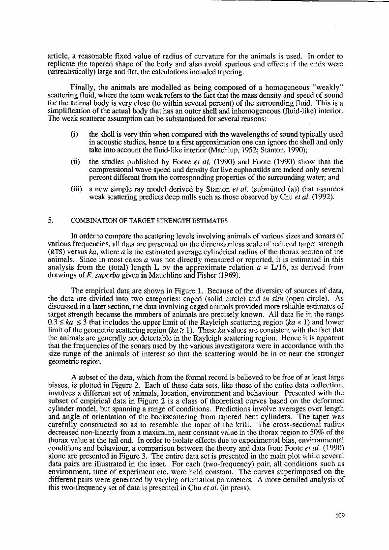
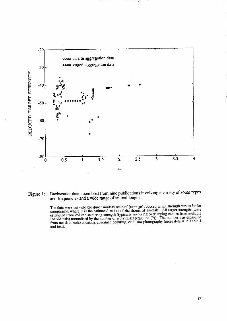
The empirical data are shown in Figure 1. Because of the diversity of sources of data, the data are divided into two categories: caged (solid circle) and in situ (open circle). As discussed in a later section, the data involving caged animals provided more reliable estimates of target strength because the numbers of animals are precisely known. All data lie in the range 0.3 ~ ka ~ 3 that includes the upper limit of the Rayleigh scattering region (ka « 1) and lower limit of the geometric scattering region (ka ~ 1). These ka values are consistent with the fact that the animals are generally not detectable in the Rayleigh scattering region. Hence it is apparent that the frequencies of the sonars used by the various investigators were in accordance with the size range of the animals of interest so that the scattering would be in or near the stronger geometric region.

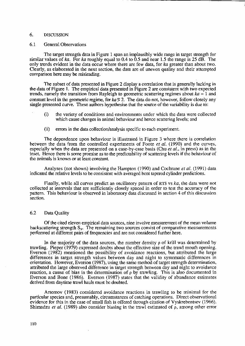
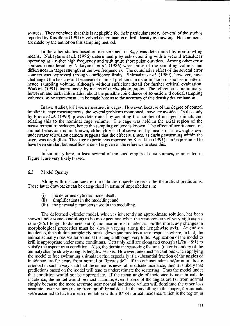
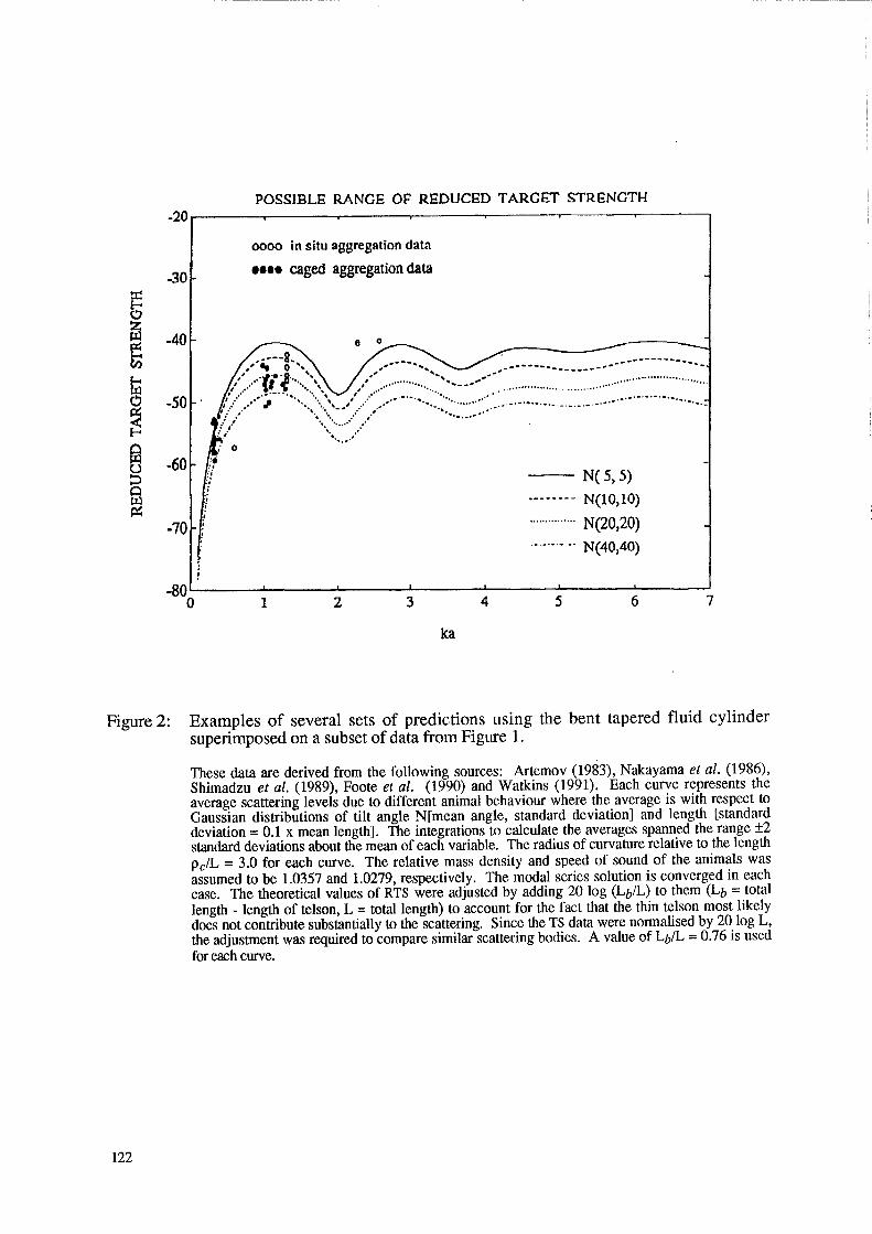
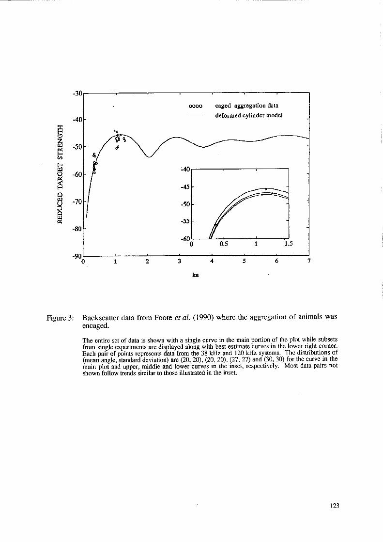
A subset of the data, which from the formal record is believed to be free of at least large biases, is plotted in Figure 2. Each of these data sets, like those of the entire data collection, involves a different set of animals, location, environment and behaviour. Presented with the subset of empirical data in Figure 2 is a class of theoretical curves based on the deformed cylinder model, but spanning a range of conditions. Predictions involve averages over length and angle of orientation of the backscattering from tapered bent cylinders. The taper was carefully constructed so as to resemble the taper of the krill. The cross-sectional radius decreased non-linearly from a maximum, near constant value in the thorax region to 50% of the thorax value at the tail end. In order to isolate effects due to experimental bias, environmental conditions and behaviour, a comparison between the theory and data from Foote et al. (1990) alone are presented in Figure 3. The entire data set is presented in the main plot while several data pairs are illustrated in the inset. For each (two-frequency) pair, all conditions such as environment, time of experiment etc. were held constant. The curves superimposed on the different pairs were generated by varying orientation parameters. A more detailed analysis of this two-frequency set of data is presented in Chu et al. (in press).

109

6. DISCUSSION

6.1 General Observations

The target strength data in Figure 1 span an implausibly wide range in target strength for similar values of ka. For ka roughly equal to 0.4 to 0.5 and near 1.5 the range is 25 dB. The only trends evident in the data occur where there are few data, for ka greater than about two. Clearly, as elaborated in the next section, the data are of uneven quality and their attempted comparison here may be misleading.

The subset of data presented in Figure 2 display a correlation that is generally lacking in the data of Figure 1. The empirical data presented in Figure 2 are consistent with two expected trends, namely the transition from Rayleigh to geometric scattering regimes about ka = 1 and constant level in the geometric regime, for ka;; 2. The data do not, however, follow closely any single presented curve. These authors hypothesise that the source of the variability is due to:

(i) the variety of conditions and environments under which the data were collected which cause changes in animal behaviour and hence scattering levels; and

(ii) errors in the data collectiOn/analysis specific to each experiment.

The dependence upon behaviour is illustrated in Figure 3 where there is correlation between the data from the controlled experiments of Foote et al. (1990) and the curves, especially when the data are presented on a case-by-case basis (Chu et al., in press) as in the inset. Hence there is some promise as to the predictability of scattering levels if the behaviour of the animals is known or at least constant.

Analyses (not shown) involving the Hampton (1990) and Cochrane et al. (1991) data indicated the relative levels to be consistent with averaged bent tapered cylinder predictions.

Finally, while all curves predict an oscillatory pattern of RTS vs ka, the data were not collected at intervals that are sufficiently closely spaced in order to test the accuracy of the pattern. This behaviour is observed in laboratory data discussed in section 4 of this discussion section.

6.2 Data Quality

Of the cited eleven empirical data sources, nine involve measurement of the mean volume backscattering strength Sv. The remaining two sources consist of comparative measurements performed at different pairs of frequencies and are not considered further here.

In the majority of the data sources, the number density p of krill was determined by trawling. Pieper (1979) expressed doubts about the effective size of the trawl mouth opening. Everson (1982) mentioned the possibility of avoidance reactions, but attributed the large differences in target strength values between day and night to systematic differences in orientation. However, Everson (1987), using the same method of target strength determination, attributed the large observed difference in target strength between day and night to avoidance reaction, a cause of bias in the determination of p by trawling. This is also documented in Everson and Bone (1986). Everson (1987) states that the validity of abundance estimates derived from daytime trawl hauls must be doubted.

Artemov (1983) considered avoidance reactions in trawling to be minimal for the particular species and, presumably, circumstances of catching operations. Direct observational evidence for this in the case of small fish is offered through citation of Vyskrebentsev (1966). Shimadzu et al. (1989) also consider biasing in the trawl estimated of p, among other error

110

sources. They conclude that this is negligible for their particular study. Several of the studies reported by Kasatkina (1991) involved detennination of krill density by trawling. No comments are made by the author on this sampling method.

In the other studies based on measurement of Sv, p was determined by non-trawling means. Nakayama et al. (1986) determined p by echo counting with a second transducer operating at a rather high frequency and with quite short pulse duration. Among other error sources considered by Nakayama et al. (1986) were those of the sampling volume and differences in target strength at the two frequencies. The cumulative effect of the several error sources was expressed through confidence limits. Shimadzu et al. (1989), however, have challenged the basic result because of claimed problems in detennination of the beam pattern, hence sampling volume, although without sufficient detail for further critical evaluation. Watkins (1991) determined p by means of in situ photography. The reference is preliminary, however, and lacks infonnation about the possible coincidence of acoustic and optical sampling volumes, so no assessment can be made here as to the accuracy of this density detennination.

In two studies, krill were measured in cages. However, because of the degree of control implicit in cage measurements, the several problems mentioned above are avoided. In the study by Foote et al. (1990), p was determined by counting the number of encaged animals and relating this to the nominal cage volume. The cage was held in the axial region of the measurement transducers, hence the sampling volume is known. The effect of confinement on animal behaviour is not known, although visual observation by means of a low-light-Ievel underwater television camera suggests that the effect at times, as during swarming within the cage, was negligible. The cage experiments reported by Kasatkina (1991) can be presumed to have been similar, but insufficient detail is given in the reference to state this.

In summary here, at least several of the cited empirical data sources, represented in Figure 1, are very likely biased.

6.3 Model Quality

Along with inaccuracies in the data are imperfections in the theoretical predictions. These latter drawbacks can be categorised in tenns of imperfections in:

(i) the defonned cylinder model itself; (ii) simplifications in the modelling; and (iii) the physical parameters used in the modelling.

The defonned cylinder model, which is inherently an approximate solution, has been shown under some conditions to be most accurate when the scatterers are of very high aspect ratio (~5:1Iength to diameter ratio) and near nonnal incidence. Furthennore, any changes in morphological properties must be slowly varying along the lengthwise axis. At end-on incidence, the solution completely breaks down and predicts a zero response where, in fact, the animal actually does scatter sound at that angle although very little. Application of the model to kriU is appropriate under some conditions. Certainly kriU are elongated enough (L/2a ~ 8: 1) to satisfy the aspect ratio condition. Also, the dominant scattering features (outer boundary of the animal) change slowly along its lengthwise axis. However, one must be cautious when applying the model to free swimming animals in situ, especially if a substantial fraction of the angles of incidence are far away from normal or "broadside". If the echo sounder and/or animals are oriented in such a way such that the animal is never at broadside incidence, then it is likely that predictions based on the model will tend to underestimate the scattering. Thus the model under that condition would not be appropriate. If the mean angle of incidence is near broadside incidence, the model would be most accurate, even if some of the angles are far from normal simply because the more accurate near nonnal incidence values will dominate the other less accurate lower values arising from far off broadside. In the modelling in this paper, the animals were assumed to have a mean orientation within 40° of normal incidence which is the region in

111

which the model is most accurate. Under this "best" condition of near normal mean incidence, high aspect ratio body, and slowly varying features, error was introduced into the modelling due to the natural approximations in the theory.

There are simplifications in the modelling of the animals. Modelling the animals as bent cylinders with or without tapering and composed of homogeneous fluid material is a great simplification of what one sees with the eye. Studies have indicated that acoustically the animals do tend to behave like bent cylinders, but nonetheless the legs, shell and inhomogeneities of the body volume were ignored in the modelling, rendering the model as being approximate at best. It is not practical, of course, to include all body parts, but ignoring even small parts builds error into the predictions.

In addition to imperfections of the mathematical aspect of the deformed cylinder solution, the information regarding physical properties of the animals is flawed hence adding another component of inaccuracy to the predictions. In order to make predictions with the model, it is essential to know the distribution of shape and orientation of the body as well as the density and speed of sound contrast of the material of the body. There are very few data concerning the distribution of orientation and no specific information on shape. Also, the information on material properties is extremely limited. All of these parameters have a profound impact on the predictions, thus it is essential that one obtains the most reliable values of the parameters for any predictions. In this article, the most reasonable values of distribution of orientation and density and speed of sound contrast were chosen although for the most part those parameter values did not involve the animals studied in the survey, hence introducing error. The shape distribution was not known at all and effects due to changes in shape were totally ignored causing more error. However, as mentioned before, simulations have shown that when the predictions are averaged over orientation, the results are relatively insensitive to the degree of bend. Hence the shape was held fixed at a reasonable mean bend.

While an exhaustive error analysis has not been performed with respect to uncertainties in the above parameters, errors introduced by the uncertainties are large enough so that final choice of the parameters must be tested by comparing predictions with scattering data whose relevant parameters are known.

6.4 Other Data

While the empirical estimates of target strength in the article involve aggregations of animals, it is useful to compare the results with crustacean zooplankton data collected in the laboratory. Although the threshold bias is greater in this latter case and the animals are of different taxa than krill, the results are quite revealing with respect to the basic physics of the scattering process. The following paragraphs review the results of Wiebe et al. (1990) and Chu et al. (1992) and compare the measurements and modelling to the results presented above.

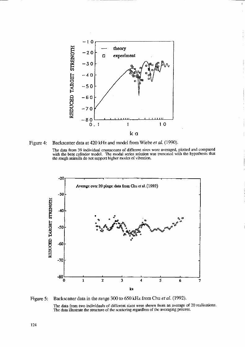
Wiebe et al. (1990) measured the backscattering of 420 kHz sound by 43 live individual macro-zooplankton and micronekton of various taxa, one of which was a euphausiid (Euphausia pacifica). All animals were crustaceans except for two of the taxa and we will limit our summary of their results to the crustaceans. The scattering measurements were conducted in a cage filled with filtered seawater deployed off a dock at Friday Harbor, Washington. The animals ranged in length from 5 to 90 mm. An attempt was made at maintaining the orientation of the animals so that either their dorsal or ventral sides were facing the transducer. This was aided by having anaesthetised all animals prior to the measurements and used an acoustically transparent tether on the larger animals. Hundreds of pings per animal were recorded so that the statistical nature of the target strengths could by analysed.

Complementing the research by Wiebe et al. (1990) is the work by Chu et al. (1992) where only two live individuals were involved (decapod shrimp - Palaemonetes vulgaris), but using a broad band sonar that covered about an octave of frequencies (300 to 650 kHz). A chirp

112

signal was used so that each animal could be insonified simultaneously with the entire range of frequencies before it had a chance to change orientation. The measurements were conducted in a seawater-filled laboratory tank at the Woods Hole Oceanographic Institution, Woods Hole, Massachusetts. The animals were 13.5 and 19.8 mm in length and were anaesthetised and tethered so that their dorsal side was facing the transducer. As a result of using a broad band sonar and two different sizes of animals, ka, where a is the cylindrical radius of the animal, spanned the values of two to six continuously. Since the amplitude of the echoes varied from ping to ping due to changes in shape and orientation of the animals, many echoes were recorded allowing a statistical analysis to be performed.

Figures 4 and 5 summarise some of the results from the studies of Wiebe et al. (1990) and Chu et al. (1992). All data involve averages over a number of pings as the animals changed shape and orientation while at the same time maintaining a principal angle of orientation (mostly via tethering) broadside to the incident acoustic signal. A truncated bent cylinder model in which the modal series solution was truncated to include just the first two modes of vibration was used to describe the Wiebe et al. (1990) data. Regardless of model, both data sets show that there is structure in the data, especially in the data collected by Chu et al. (1992). In the latter data set, there is a distinct dip in the data at the ka = 2 and 3.5 values - the positions of which are predicted by the fluid cylinder theory (the dips were confirmed in a more complete experiment by Stanton et al. (submitted (b)). The structure in the Wiebe et al. (1990) data set is less pronounced although a dip is suggested in the ka = 2 region.

While the overall levels and/or general trends of these laboratory data sets may not coincide exactly with the target strength estimates presented in Figure 1 (the reasons possibly due to thresholding effects discussed earlier in this article and differences in animal type), the structure exhibited in the laboratory data sets is important. In a figure not presented here involving single (un averaged) echoes, Chu et al. (1992) show that this dip can be quite distinct and is sometimes as much as 30 dB below the levels of the scattering at surrounding values of ka. In spite of the effects of averaging the echo over distributions of angle of orientation and length which tend to "smear" out the nuUs, there is still some residual dip that is of the order 5 to 7 dB below the surrounding values. As shown in Stanton et al. (submitted (a)) the presence of the dips is due to interference between the echoes from the front and back interfaces of the animals. The smearing effect has been successfully modelled in Stanton et al. (submitted (b)). It is quite apparent from the laboratory studies that the Ts/length relationship for zooplankton is not monotonic.

7. SUMMARY, CONCLUSION AND RECOMMENDATIONS

An attempt has been made to specify the target strength of krill through reference to a particular kind of measurement and by exercise of a scattering model. To avoid possible threshold-induced bias with single-animal measurements, only measurements on aggregations have been used. Many of these, however, have depended on physical sampling by trawl in order to determine the number density of observed krill. Because of the generally unknown effect of such sampling on the targeted animals, related acoustic measurements dependent on trawling must be suspected. The data collected by Kasatkina (1991) and Watkins (1991) are not considered further here because of their admitted or evident preliminary state of publication. Only some of the cited empirical data sources thus remain as candiates for use. These are those by Foote et al. (1990), Hampton (1990), and Cochrane et al. (1991). The measurement methods described by Nakayama et al. (1986) and Watkins (1991) are also potentially valuable, as would be the direct dual-beam or split-beam measurement methods, of which the first split-beam measurements have recently been reported by Hewitt and Demer (1991).

Numerical computation by means of the theoretical scattering model (Stanton, 1989) offers an attractive alternative to measurement, especially as the model is not limited to a particular size or frequency range. However, the model does depend on a knowledge of the animal's physical properties, e.g., mass densities of and sound speeds in muscle and other

113

tissue, in addition to morphometry. To relate the result of computations to measurements in the wild, it is also necessary to know something about the orientation characteristics of kriU during the conditions of surveying. In the present work, values for the physical properties and orientation distribution have been assigned according to independent measurements. Unfortunately, the degree to which these parameter values are representative is unknown.

The authors thus find themselves in the classic dilemma of wanting to solve a problem -specification of the target strength of krill - for which there are few plausible direct measurements and for which a plausible theoretical model lacks basic data on its underlying parameters, which are required for its proper exercise. A provisional resolution is, however, suggested.

The empirical data collected by Foote et al. (1990) seem to escape the major problems associated with many other data on kriU target strength. The cited data apply strictly to encaged E. superba. Hampton (1990) has performed extensive, comparative measurements on the same species in situ and at the same frequencies of 38 and 120 kHz. The difference in target strength at the two frequencies is the same for the measurements on encaged and wild aggregations. Additional in situ measurements, performed at 50 and 200 kHz on M eganyctiphanes norvegica by Cochrane et al. (1991), support the same general finding. Given that the model calculations with averaging show a fair agreement with these measurements, the following conclusion is drawn.

7.1 Conclusion

For the time being, in the absence of new data, the target strength of krill may be determined from the curves shown in Figure 2. Since this displays the reduced target strength as a function of ka, an absolute target strength must be derived for the particular application, hence frequency and animal size, according to equation (3). Lacking more detailed data, the size parameter a may be determined from the measured total length L by the relation a ~ L/16.

To address the various shortcoming noted above, the following recommendations are made for improved determinations of krill target strength in the future:

114

(i) measurements of the kinds reported by Foote et al. (1990), Hampton (1990), and Cochrane et al. (1991) should be repeated for a wider range of animal sizes and frequencies;

(ii) measurements of the kind reported by Nakayama et al. (1986) should be performed with particular care being given to the sampling volume of the second, high-frequency, short-pulse transducer used to determine number density by echo counting;

(iii) measurements should be made using dual-beam or split-beam echo sounding systems;

(iv) the physical properties of krill should be measured: (a) whenever possible to determine the range of variation in such properties and causative mechanisms; and, (b) in conjunction with studies performed along the lines of recommendations (i) to (iii); and

(v) the orientation and shape characteristics of krill should be determined whenever possible, especially under conditions when the animal would be surveyed.

ACKNOWLEDGEMENTS

The authors would like to thank Shirley Bowman of the Woods Hole Oceanographic Institution, Woods Hole, MA, for preparing the manuscript to this article. Ken Foote wishes to express his appreciation to WHOI for its invitation to visit, summer 1991. This research was supported by the Institute of Marine Research, Bergen, Norway, the US Office of Naval Research grant number NOOOI4-89-J-1729, and the US Naval Underwater Systems Center contract number N66604-91-C-5401. This is Woods Hole Oceanographic Institution contribution number 7890.

REFERENCES

ANON. 1986. Report on Post-FIBEX Acoustic Workshop, Frankfurt, 3-14 September 1984. BIOMASS Report Series, 40: 126 pp.

ARTEMOV, A.T. 1983. Determination of the acoustic back scatter cross section of small pelagic organisms in aggregations. Oceanology,23: 264-266.

CHU, D., T.K. STANTON AND P.H. WIEBE. 1992. Frequency dependence of sound backscattering from live individual zooplankton. ICES Journal of Marine Science, 49: 97-106.

CHU, D., T.K. STANTON AND K.G. FOOTE. (In press). Further analysis of target strength measurements of Antarctic krill at 38 kHz and 120 kHz: comparison with deformed cylinder model and inference of orientation distribution. Journal of the Acoustical Society of America.

COCHRANE, N.A., D. SAMEOTO, A.W. HERMAN AND J. NEILSON. 1991. Multiple-frequency acoustic backscattering and zooplankton aggregations in the inner Scotian Shelf basins. Canadian Journal of Fisheries and Aquatic Science, 48: 340-355.

ENDO, Y. 1989. Swim angles of Euphausia pacifica. Proc. NIPR Symposium on Polar Biology, 2: 219 pp.

EVERSON, I. 1982. Diurnal variations in mean volume backscattering strength of an Antarctic krill (Euphausia superba) patch. Journal Plankton Research, 4: 155-162.

EVERSON, I. 1987. Some aspects of the small scale distribution of Euphausia superba. Polar Biology, 8: 9-15.

EVERSON, I. and D.G. BONE. 1986. Effectiveness of the RMT8 system for sampling krill (Euphausia superba) swarms. Polar Biology, 6: 83-90.

FOOTE, K.G. 1982. Optimising copper spheres for precision calibration of hydroacoustic equipment. Journal of the Acoustical Society of America, 71: 742-747.

FOOTE, K.G. 1990. Speed of sound in Euphausia superba. Journal of the Acoustical Society of America, 87: 1405-1408.

FOOTE, K.G., A. AGLEN and o. NAKKEN. 1986. Measurement of fish target strength with a split-beam echosounder. Journal of the Acoustical Society of America, 80: 612-621.

FOOTE, K.G., I. EVERSON, J.L. WATKINS and D.G. BONE. 1990. Target strengths of Antarctic krill (Euphausia superba) at 38 kHz and 120 kHz. Journal of the Acoustical Society of America, 87: 16-24.

115

FORBES, S.T. and o. NAKKEN. 1972. Manual of methods for fisheries resource survey and appraisal. Part 2. The use of acoustic instruments for fish detection and abundance estimation. FAO Man. Fish. Science, 5: 1-138.

HAMPTON, I. 1990. Measurements of differences in the target strength of Antarctic krill (E. superba) swarms at 38 and 120 kHz. In: Selected Scientific Papers, 1990. (SC-CAMLR-SSP/7). CCAMLR, Hobart, Australia: 75-86.

HEWITT, R.P. and D.A. DEMER. 1991. Krill abundance. Nature, 353: 310 pp.

KASATKINA, S.M. 1991. Target strengths of krill at 136 and 20 kHz. In: Selected Scientific Papers, 1991 (SC-CAMLR-SSP/S). CCAMLR, Hobart, Australia: 141-157.

KILS, u. 1979. Preliminary data on volume, density and cross section area of Antarctic krill, Euphausia superba. Meeresforsch, 27: 207-209.

KILS, u. 1981. The swimming behaviour, swimming performance and energy balance of Antarctic krill, Euphausia superba. BIOMASS Science Series, 3: 122 pp.

KRISTENSEN, A. and J. DALEN. 1986. Acoustic estimation of size distribution and abundance of zooplankton. Journal of the Acoustical Society of America, 80: 60 1-611.

MACLENNAN, D.N. 1990. Acoustical measurement of fish abundance. Journal of the Acoustical Society of America, 87: 1-15.

MACHLUP, S. 1952. A theoretical model for sound scattering by marine crustaceans. Journal of the Acoustical Society of America, 24: 290-293.

MAUCHLINE, J. and L.R. FISHER. 1969. The biology of euphausiids. In: RUSSEL, F.R. and M. YONGE (Eds.). Advances in Marine Biology. Chapter 7. Academic Press, London.

MILLER, D.G.M. and I. HAMPTON. 1989. Biology and ecology of the Antarctic krill (Euphausia superba Dana). A review. BIOMASS Science Series, 9: 166 pp.

NAKAYAMA, K., K. SHIRAKIHARA and Y. KOMAKI. 1986. Target strength ofkrill in situ at the frequency of 200 kHz. Memorial National Institute of Polar Research, Special Issue 40: 153-161.

PIEPER, R.E. 1979. Euphausiid distribution and biomass determined acoustically at 102 kHz. Deep-Sea Research, 26: 687-702.

SAMEOTO, D.D. 1980; Quantitative measurements of euphausiids using a 120 kHz sounder and their in situ orientation. Canadian Journal of Fisheries and Aquatic Science, 37: 693-702.

SHIMADZU, Y., T. KIOKE and T. SUGURO. 1989. Target strength estimation of Antarctic krill, Euphausia superba by cooperative experiments with commercial trawler. Document SC-CAMLR-VIII/BG/30. CCAMLR, Hobart, Australia: 10 pp.

STANTON, T.K. 1989. Sound scattering by cylinders of finite length. Ill. Deformed Cylinders. Journal of the Acoustical Society of America, 86: 691-705.

STANTON, T.K. 1990. Sound scattering by spherical and elongated shelled bodies. Journal of the Acoustical Society of America, 88: 1619-1633.

116

STANTON, T.K., C.S. CLAY and D. CHU. Submitted (a). Ray representation of sound scattering by weakly scattering deformed fluid cylinders: simple physics and application to zooplankton. Journal of the Acoustical Society of America.

STANTON, T.K., D. CRU, P.R. WIEBE and C.S. CLAY. Submitted (b). Average echoes from randomly-oriented random-length finite cylinders: zooplankton models. Journal of the Acoustical Society of America.

STANTON, T.K., RD.M. NASR, R.L. EASTWOOD and R.W. NERO. 1987. A field examination of acoustical scattering from marine organisms at 70 kHz. IEEE Journal of Oceanic Engineering OE-12: 339-348.

URICK, R.J. 1975. Principles of Underwater Sound. 2nd Edition. McGraw-Hill, New York: 384 pp.

VYSKREBENTSEV, B.V. 1966. Observations of the operations of trawl nets in the Black Sea. Tr. Okeanograf. kommissii AN USSR, 14: 187-196.

WATKINS, J.L. 1991. Krill target strength estimated by underwater photography and acoustics. Document WG-Krill-9JI40. CCAMLR, Hobart, Australia.

WEIMER, R.T. and J.E. EHRENBERG. 1975. Analysis of threshold-induced bias inherent in acoustic scattering cross-section estimates of individual fish. Journal of the Fisheries Research Board Canada, 32: 2547-2551.

WIEBE, P.R., C.R. GREENE, T.K. STANTON and J. BURCZYNSKI. 1990. Sound scattering by live zooplankton and micronekton: empirical studies with a dual-beam acoustical system. Journal of the Acoustical Society of America, 88: 2346-2360.

117

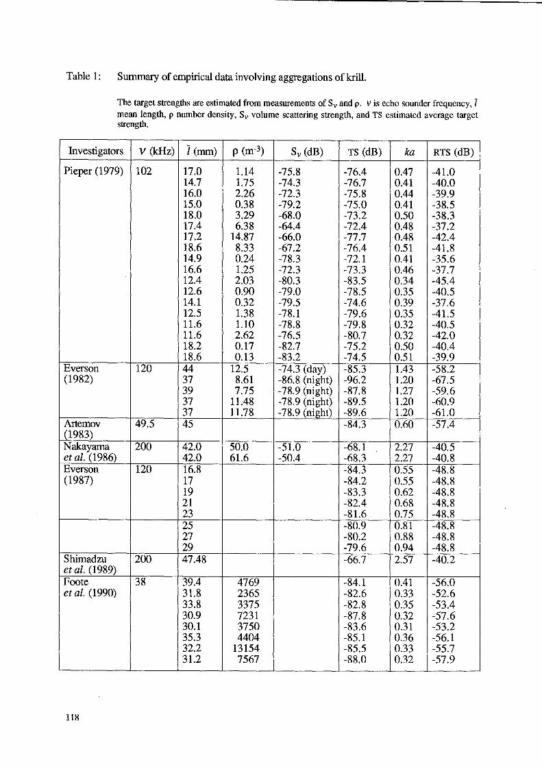
Table 1: Summary of empirical data involving aggregations of kriU.

The target strengths are estimated from measurements of Sv and p. V is echo sounder frequency, I mean length, p number density, Sv volume scattering strength, and TS estimated average target strength.

Investigators V (kHz) i (mm) p (m-3) Sv (dB) TS (dB) ka RTS (dB)

Pieper (1979) 102 17.0 1.14 -75.8 -76.4 0.47 -41.0 14.7 1.75 -74.3 -76.7 0.41 -40.0 16.0 2.26 -72.3 -75.8 0.44 -39.9 15.0 0.38 -79.2 -75.0 0.41 -38.5 18.0 3.29 -68.0 -73.2 0.50 -38.3 17.4 6.38 -64.4 -72.4 0.48 -37.2 17.2 14.87 -66.0 -77.7 0.48 -42.4 18.6 8.33 -67.2 -76.4 0.51 -41.8 14.9 0.24 -78.3 -72.1 0.41 -35.6 16.6 1.25 -72.3 -73.3 0.46 -37.7 12.4 2.03 -80.3 -83.5 0.34 -45.4 12.6 0.90 -79.0 -78.5 0.35 -40.5 14.1 0.32 -79.5 -74.6 0.39 -37.6 12.5 1.38 -78.1 -79.6 0.35 -41.5 11.6 1.10 -78.8 -79.8 0.32 -40.5 11.6 2.62 -76.5 -80.7 0.32 -42.0 18.2 0.17 -82.7 -75.2 0.50 -40.4 18.6 0.13 -83.2 -74.5 0.51 -39.9

Everson 120 44 12.5 -74.3 (day) -85.3 1.43 -58.2 (1982) 37 8.61 -86.8 (night) -96.2 1.20 -67.5

39 7.75 -78.9 (night) -87.8 1.27 -59.6 37 11.48 -78.9 (night) -89.5 1.20 -60.9 37 11.78 -78.9 (night) -89.6 1.20 -61.0

Artemov 49.5 45 -84.3 0.60 -57.4 (1983) Nakayama 200 42.0 50.0 -51.0 -68.1 2.27 -40.5 et al. (1986) 42.0 61.6 -50.4 -68.3 2.27 -40.8 Everson 120 16.8 -84.3 0.55 -48.8 (1987) 17 -84.2 0.55 -48.8

19 -83.3 0.62 -48.8 21 -82.4 0.68 -48.8 23 -81.6 0.75 -48.8 25 -80.9 0.81 -48.8 27 -80.2 0.88 -48.8 29 -79.6 0.94 -48.8

Shimadzu 200 47.48 -66.7 2.57 -40.2 et al. (1989) Foote 38 39.4 4769 -84.1 0.41 -56.0 et al. (1990) 31.8 2365 -82.6 0.33 -52.6

33.8 3375 -82.8 0.35 -53.4 30.9 7231 -87.8 0.32 -57.6 30.1 3750 -83.6 0.31 -53.2 35.3 4404 -85.1 0.36 -56.1 32.2 13154 -85.5 0.33 -55.7 31.2 7567 -88.0 0.32 -57.9

118

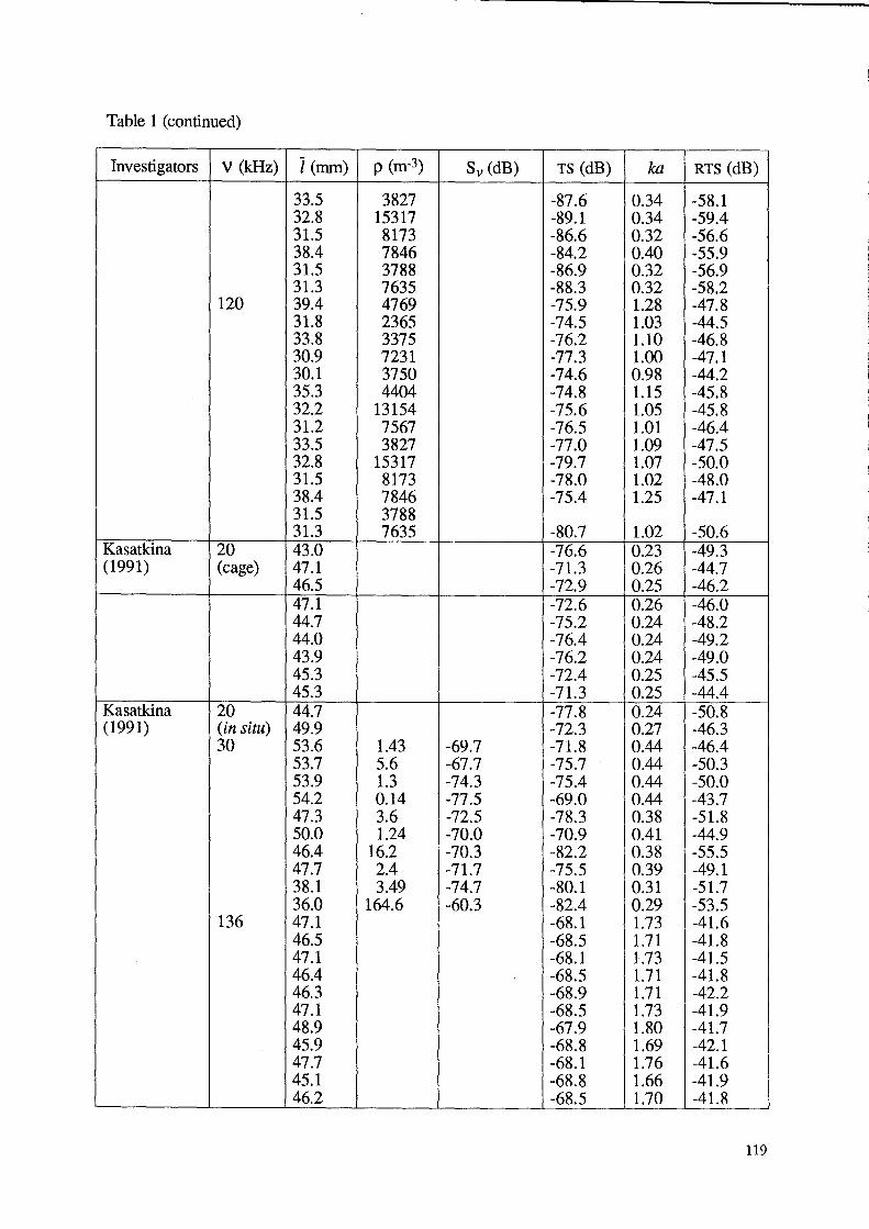
Table 1 (continued)

Investigators V (kHz) I (mm) p (m-3) Sv (dB) TS (dB) ka RTS(dB)

33.5 3827 -87.6 0.34 -58.1 32.8 15317 -89.1 0.34 -59.4 31.5 8173 -86.6 0.32 -56.6 38.4 7846 -84.2 0.40 -55.9 31.5 3788 -86.9 0.32 -56.9 31.3 7635 -88.3 0.32 -58.2

120 39.4 4769 -75.9 1.28 -47.8 31.8 2365 -74.5 1.03 -44.5 33.8 3375 -76.2 1.10 -46.8 30.9 7231 -77.3 1.00 -47.1 30.1 3750 -74.6 0.98 -44.2 35.3 4404 -74.8 1.15 -45.8 32.2 13154 -75.6 1.05 -45.8 31.2 7567 -76.5 1.01 -46.4 33.5 3827 -77.0 1.09 -47.5 32.8 15317 -79.7 1.07 -50.0 31.5 8173 -78.0 1.02 -48.0 38.4 7846 -75.4 1.25 -47.1 31.5 3788 31.3 7635 -80.7 1.02 -50.6

Kasatkina 20 43.0 -76.6 0.23 -49.3 (1991) (cage) 47.1 -71.3 0.26 -44.7

46.5 -72.9 0.25 -46.2 47.1 -72.6 0.26 -46.0 44.7 -75.2 0.24 -48.2 44.0 -76.4 0.24 -49.2 43.9 -76.2 0.24 -49.0 45.3 -72.4 0.25 -45.5 45.3 -71.3 0.25 -44.4

Kasatkina 20 44.7 -77.8 0.24 -50.8 (1991) (in situ) 49.9 -72.3 0.27 -46.3

30 53.6 1.43 -69.7 -71.8 0.44 -46.4 53.7 5.6 -67.7 -75.7 0.44 -50.3 53.9 1.3 -74.3 -75.4 0.44 -50.0 54.2 0.14 -77.5 -69.0 0.44 -43.7 47.3 3.6 -72.5 -78.3 0.38 -51.8 50.0 1.24 -70.0 -70.9 0.41 -44.9 46.4 16.2 -70.3 -82.2 0.38 -55.5 47.7 2.4 -71.7 -75.5 0.39 -49.1 38.1 3.49 -74.7 -80.1 0.31 -51.7 36.0 164.6 -60.3 -82.4 0.29 -53.5

136 47.1 -68.1 1.73 -41.6 46.5 -68.5 1.71 -41.8 47.1 -68.1 1.73 -41.5 46.4 -68.5 1.71 -41.8 46.3 -68.9 1.71 -42.2 47.1 -68.5 1.73 -41.9 48.9 -67.9 1.80 -41.7 45.9 -68.8 1.69 -42.1 47.7 -68.1 1.76 -41.6 45.1 -68.8 1.66 -41.9 46.2 -68.5 1.70 -41.8

119

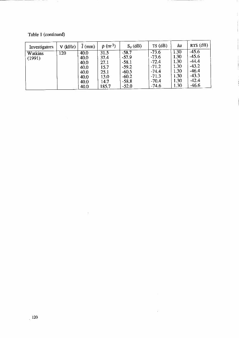
Table 1 (continued)

Investigators V (kHz) 1 (mm) p (m-3) Sv(dB) TS (dB) ka RTS (dB)

Watkins 120 40.0 31.5 -58.7 -73.6 1.30 -45.6

(1991) 40.0 37.4 -57.9 -73.6 1.30 -45.6 40.0 27.1 -58.1 -72.4 1.30 -44.4 40.0 15.7 -59.2 -71.2 1.30 -43.2 40.0 25.1 -60.5 -74.4 1.30 -46.4 40.0 13.0 -60.2 -71.3 1.30 -43.3 40.0 14.7 -58.8 -70.4 1.30 -42.4 40.0 185.7 -52.0 -74.6 1.30 -46.6

120

-20

0000 in situ aggregation data

-30 •••• caged aggregation data

~ 0

Z 006'0 III -40 aJ c;l:JJJ. 0 r: 6' 0 0 8

.",.

CJl 0 •• t 000

0

fil ,.,. .8 , 0000000 • •

C> -50 0 0 0 ••

~ 00 ~.

E-< r ®

0 0

-60 • 0 . 0

~ @ c::=:: 0

-70 .

_80~----~----~----~------L-----~----~----~----~ 1.5 2 2.5 3 3.5 4 o 0.5 1

ka

Figure 1: Backscatter data assembled from nine publications involving a variety of sonar types and frequencies and a wide range of animal lengths.

The data were put onto the dimensionless scale of (average) reduced target strength versus ka for comparison where a is the estimated radius of the thorax of animals. All target strengths were estimated from volume scattering strength (typically involving overlapping echoes from multiple individiuals) normalised by the number of i~dividuals (equation (9)). The number was estimated from net data, echo counting, specimen counting, or in situ photography (more details in Table 1 and text).

121

POSSIBLE RANGE OF REDUCED TARGET STRENGTH -20r-----~------~----~------~----~------~----~

-30

-40

-50 .

, -70 f

0000 in situ aggregation data

•••• caged aggregation data

,-·--R. ,'" 0 .... ' .-,,------ ... -- __ • ___ - .... --- .... ------ ..... ...

"" ... ···!i· ~ ....... ' ... \, ................. .0 ..................... ,.' ••••• , ••••••• n

................... .

::;;:::. "~"'" ::~::2:::::::'"'''' ":: :::::::: .......- . ................ .. ........ . .......

N( 5,5)

N(lO,lO)

N(20,20) .......... N(40,40)

-80 "---__ -'--__ -'-__ --...I. ___ ..L.-. __ ...J.-__ ----L __ -J

4 5 6 7 o 1 2 3

Figure 2: Examples of several sets of predictions using the bent tapered fluid cylinder superimposed on a subset of data from Figure 1.

122

These data are derived from the following sources: Artemov (1983), Nakayama et al. (1986), Shimadzu et al. (1989), Foote et al. (1990) and Watkins (1991). Each curve represents the average scattering levels due to different animal behaviour where the average is with respect to Gaussian distributions of tilt angle N[mean angle, standard deviation] and length [standard deviation = 0.1 x mean length]. The integrations to calculate the averages spanned the range ±2 standard deviations about the mean of each variable. The radius of curvature relative to the length PcIL = 3.0 for each curve. The relative mass density and speed of sound of the animals was assumed to be 1.0357 and 1.0279, respectively. The modal series solution is converged in each case. The theoretical values of RTS were adjusted by adding 20 log (LbIL) to them (Lb = total length - length of telson, L = total length) to account for the fact that the thin telson most likely does not contribute substantially to the scattering. Since the TS data were normalised by 20 log L, the adjustment was required to compare similar scattering bodies. A value of LbIL = 0.76 is used for each curve.

-30

0000 caged aggregation data

-40 deformed cylinder model

§ Z u:I ~

t;

tl 0

~ Cl tj ;J Q ~ ~ -55

-80

-60 0 0.5 1 ,1.5

-90 0 1 2 3 4 5 6 7

ka

Figure 3: Backscatter data from Foote et al. (1990) where the aggregation of animals was encaged.

The entire set of data is shown with a single curve in the main portion of the plot while subsets from single experiments are displayed along with best-estimate curves in the lower right corner. Each pair of points represents data from the 38 kHz and 120 kHz systems. The distributions of (mean angle, standard deviation) are (20, 20), (20,20), (27, 27) and (30, 30) for the curve in the main plot and upper, middle and lower curves in the inset, respectively. Most data pairs not shown follow trends similar to those illustrated in the inset.

123

-to

§ -20 theory

! 0 experiment

-30

fil -40 0

~ -50

0 -60

~ -70 fij ~

-80 O. 1 0

ka Figure 4: Backscatter data at 420 kHz and model from Wiebe et al. (1990).

The data from 39 individual crustaceans of different sizes were averaged, plotted and compared with the bent cylinder model. The modal series solution was truncated with the hypothesis that the rough animals do not support higher modes of vibration.

-20r-----~----_r----~------r_----~----~----~

-30

-40

-50

-60

-70

Ave:rage: ove:r 20 pings: data Crom Chu et al. (1992)

o o

Figure 5: Backscatter data in the range 300 to 650 kHz from Chu et al. (1992).

124

The data from two individuals of different sizes were shown from an average of 20 realisations. The data illustrate the structure of the scattering regardless of the averaging process.

Tableau 1:

Figure 1:

Figure 2:

Figure 3:

Figure 4:

Figure 5:

Ta6JIHI..\a 1:

PHCYHOK 1:

PHCYHOK 2:

PHCYHOK 3:

PHCYHOK 4:

Ugende des tableaux

Recapitulation des donnees empiriques concernant les concentrations de krill.

Legende des figures

Donnees de retrodiffusion proven ant de neuf publications concern ant differents types et frequences d'echosondeurs et un intervalle important de longueurs d'animaux.

Exemples de plusieurs jeux de predictions utilisant le cylindre de fluide coude et en fuseau, superpose a un sous-jeu de donnees de la Figure 1, a savoir celles derivees des sources suivantes: Artemov (1983), Nakayama et al. (1986), Shimadzu et al. (1989), Foote et al. (1990) et Watkins (1991).

Donnees de retrodiffusion de Foote et al. (1990) lorsque les concentrations etaient en enceinte.

Donnees de retrodiffusion a 420 kHz et modele de Wiebe et al. (1990) dans lequel on a etabli la moyenne, on les a tracees et comparees des donnees de 39 individus de crustaces de tailles differentes au modeIe de cylindre coude.

Donnees de retrodiffusion comprises dans l'intervalle de 300 a 650 kHz de Chu et al. (1992) dans lesquelles les donnees de deux individus de differentes tailles sont presentees sur une moyenne de 20 essais.

CnHCOK Ta6JIHI..\

CBO.llKa 3MnHpIF.leCKHX .llaHHbIX, nOJIY4eHHbIX Ha CKOnJIeHH5IX KPHJI5I.

CnHCOK PHCYHKOB

llaHHble no aKYCTH4eCKOMY pacceHBaHHIO H3 .lleB5ITH ny6JIHKaI..\HM,

KacaIOII(HeC5I p5I.lla THnOB rH.llpOJIOKaTOpOB, HX 4aCTOT H IIIHpOKoro

.llHana30Ha .llJIHH )l{HBOTHbIX.

I1pHMepbI HeCKOJIbKHX BapHaHTOB nporH030B C HCnOJIb30BaHHeM

,l{e<popMHpOBaHHoro I..\HJIHH.llpa, HaJIO)l{eHHbIX Ha 4aCTH4HbIM Ha60p

.llaHHbIX H3 PHCYHKa 1. BbIJIH HCnOJIb30BaHbI .llaHHble CJIe.llYIOII(HX

aBTopOB: Artemov (1983), Nakayama et al. (1986), Shimadzu et al. (1989), Foote et al. (1990) H Watkins (1991).

llaHHble no aKycTH4ecKoMY pacceHBaHHIO H3 pa60TbI cDYT H .llp.

(Foote et al., 1990) - CKOnJIeHHe oc06eM HaX0.llHJIOCb B ca.llKe.

llaHHble no aKycTH4ecKoMY pacceHBaHHIO Ha 4aCTOTe 420 Krl..\ H

MO.lleJIb H3 pa60TbI BH6e H .llp. (Wiebe et al.,1990) - 6bIJIH ycpe.llHeHbI,

HaHeceHbl Ha rpa<pHK H cpaBHeHbI C MO.lleJIbIO pacceHBaHH5I

.lle<popMHpOBaHHbIX I..\HJIHH.llPOM. llaHHble no 39 OT .lleJIbHbIM pa4KaM

pa3HOrO pa3Mepa.

125

PHCYHOK 5:

Tabla 1:

Figura 1:

Figura 2:

Figura 3:

Figura 4:

Figura 5:

126

llaHHbIe no aKYCTHlIeCKOMY pacceHBaHHIO B ,l\Hana30He 300 - 650 KrU;

H3 pa60TbI lly H ,l\p. (Chu et al., 1992) - nOKa3aHbI ,l\aHHbIe no ,l\BYM

OC06S1M pa3HOrO pa3Mepa, OCpe,l\HeHHbIe no pe3YJIbTaTaM 20 nporoHoB. HeCMOTpSl Ha HCnOJIb3yeMoe ycpe,l\HeHHe 3TH ,l\aHHbIe

HJIJIIOCTPHPYIOT CTpyKTypy pacceHBaHHSI.

Lista de las tablas

Resumen de datos empfricos de las concentraciones de kril.

Lista de las figuras

Series de datos de retrodispersi6n de nueve publicaciones, en las que se utilizaron distintos tipos de sonar, frecuencias y animales de distinta talla.

Ejemplos de varias series de predicciones mediante el cilindro curvado superpuesto en una subserie de datos de la figura 1.

Datos de retrodispersi6n de Foote et al. (1990) de concentraciones encerradas.

Datos de retrodispersi6n a 420 kHz y modelo de Wiebe et al. (1990).

Datos de retrodispersi6n entre 300 a 650 kHz de Chu et al. (1992).